PART

THREE PERTURBATION METHODS

When I hear you give your reasons, the thing always appears to me to be so ridiculously simple that I could easily do it myself, though at each successive instance of your reasoning I am baffled until you explain your process.

-Dr. Watson, A Scandal in Bohemia

Sir Arthur Conan Doyle

The local analysis methods of Part II are powerful tools, but they cannot provide global information on the behavior of solutions at two distantly separated points. They cannot predict how a change in initial conditions at x = 0 will affect the asymptotic behavior as x ~ + 00. To answer such questions we must apply the methods of global analysis which will be developed in Part IV. Since global methods are perturbative in character, in this part we will first introduce the requisite mathematical concepts: perturbation theory in Chap. 7 and summa­tion theory in Chap. 8.

Perturbation theory is a collection of methods for the systematic analysis of the global behavior of solutions to differential and difference equations. The gen­eral procedure of perturbation theory is to identify a small parameter, usually denoted by 8, such that when 8 = 0 the problem becomes soluble. The global solution to the given problem can then be studied by a local analysis about 8 = O. For example, the differential equation y" = [1 + 8/(1 + x 2 )]y can only be solved in terms of elementary functions when 8 = O. A perturbative solution is constructed by local analysis about 8 = 0 as a series of powers of 8:

y(x) = Yo(x) + 8Yl(X) + 82Y2(X) + .... This series is called a perturbation series. It has the attractive feature that Yn(x) can be computed in terms of Yo(x), ... , Yn- 1 (X) as long as the problem obtained by setting 8 = 0, y" = y, is soluble, which it is in this case. Notice that the pertur­bation series for y(x) is local in 8 but that it is global in x. If 8 is very small, we expect that y(x) will be well approximated by only a few terms of the perturbation series.

317

318 PERTURBATION METHODS

The local analysis methods of Part II are other examples of perturbation theory. There the expansion parameter is t; = x - Xo or t; = l/x if Xo = 00.

Perturbation series, like asymptotic expansions, often diverge for all t; =1= O. However, since t; is not necessarily a small parameter, the optimal asymptotic approximation may give very poor numerical results. Thus, to extract maximal information from perturbation theory, it is necessary to develop sophisticated techniques to "sum" divergent series and to accelerate the convergence of slowly converging series. Methods to achieve these goals are presented in Chap. 8. Sum­mation methods also apply to the local series expansions derived in Part II.

In perturbation theory it is convenient to have an asymptotic order relation that expresses the relative magnitudes of two functions more precisely than « but less precisely than "'. We define

f(x) = O[g(x)], x -+ XO,

and say ''f(x) is at most of order g(x) as x -+ xo" or ''f(x) is '0' of g(x) as x -+ xo" iff(x)!g(x) is bounded for x near Xo; that is, If(x)/g(x)1 < M, for some constant M if x is sufficiently close to Xo' Observe that iff(x) '" g(x) or iff(x)« g(x) as x -+ xo, thenf(x) = O[g(x)] as x -+ Xo. Iff« g as x -+ xo, then any M > 0 satisfies the definition, while iff'" g (x -+ xo), only M > 1 can work.

In perturbation theory one may calculate just a few terms in a perturbation series. Whether or not this series is convergent, the notation "0" is very useful for expressing the order of magnitude of the first neglected term when that term has not been calculated explicitly.

Examples

1. x sin x = O(x) (x --->0 or x ---> ex:»; 2. e- I /x = O(x") (x ---> 0+) for all n; 3. x5 = O(X2) (x ---> 0+); 4. eX = 1 + x + (x 2/2) + O(x3) (x ---> 0); 5. Ai (x) = !1t-1/2x-I/4e-2x3!'!3[1 - ~x- 3/2 + O(x- 3)] (x -+ + ex:».

CHAPTER

SEVEN PERTURBATION SERIES

You have erred perhaps in attempting to put colour and life into each of your statements instead of confining yourself to the task of placing upon record that severe reasoning from cause to effect which is really the only notable feature about the thing. You have degraded what should have been a course of lectures into a series of tales.

-Sherlock Holmes, The Adventure of the Copper Beeches

Sir Arthur Conan Doyle

(E) 7.1 PERTURBATION THEORY

Perturbation theory is a large collection of iterative methods for obtaining approximate solutions to problems involving a small parameter e. These methods are so powerful that sometimes it is actually advisable to introduce a parameter e temporarily into a difficult problem having no small parameter, and then finally to set e = 1 to recover the original problem. This apparently artificial conversion to a perturbation problem may be the only way to make progress.

The thematic approach of perturbation theory is to decompose a tough prob­lem into an infinite number of relatively easy ones. Hence, perturbation theory is most useful when the first few steps reveal the important features of the solution and thl;! remaining ones give small corrections.

Here is an elementary example to introduce the ideas of perturbation theory.

Example 1 Roots of a cubic polynomial. Let us find approximations to the roots of

X3 - 4.00lx + 0.002 = o. (7.1.1 )

As it stands, this problem is not a perturbation problem because there is no small parameter e. It may not be easy to convert a particular problem into a tractable perturbation problem, but in the present case the necessary trick is almost obvious. Instead of the single equation (7.1.1) we consider the one-parameter family of polynomial equations

x 3 - (4 + e)x + 2e = O. (7.1.2)

When e = 0.001, the original equation (7.1.1) is reproduced. It may seem a bit surprising at first, but it is easier to compute the approximate roots of the

family of polynomials (7.1.2) than it is to solve just the one equation with e = 0.001. The reason

319 C. M. Bender et al., Advanced Mathematical Methods for Scientists and Engineers I© Springer Science+Business Media New York 1999

320 PERTURBATION METHODS

for this is that if we consider the roots to be functions of e, then we may further assume a perturbation series in powers of e:

x(e) = L a.e·. n=O

To obtain the first term in this series, we set e = 0 in (7.1.2) and solve

X3 - 4x = O.

(7.1.3)

(7.1.4)

This expression is easy to factor and we obtain in zeroth-order perturbation theory x(O) = ao = -2,0,2.

A second-order perturbation approximation to the first of these roots consists of writing (7.1.3) as XI = -2 + ale + a2 e2 + 0(e3 ) (e ..... O), substituting this expression into (7.1.2), and neglecting powers of e beyond e2 • The result is

(-8 + 8) + (12a l - 4a l + 2 + 2)e + (12a 2 - a l - 6ai - 4a2 )e2 = 0(e3 ), e ..... O. (7.1.5)

It is at this step that we realize the power of generalizing the original problem to a family of problems (7.1.2) with variable e. It is because e is variable that we can conclude that the coefficient of each power of e in (7.1.5) is separately equal to zero. This gives a sequence of equations for the expansion coefficients aI' a2' ... :

el : 8al + 4 = 0; e2: 8a2 - al - 6ai = 0;

and so on. The solutions to the equations are al = -i, a2 = !, .... Therefore, the perturbation expansion for the root XI is

X I = - 2 - ie + !e2 + .... (7.1.6)

If we now set e = 0.001, we obtain XI from (7.1.6) accurate to better than one part in 109.

The same procedure gives

X2 = 0 + ie - ie2 + 0(e3 ), X3 = 2 + O'e + 0'e 2 + 0(e3 ), e ..... O.

(Successive coefficients in the perturbation series for X3 all vanish because X3 = 2 is the exact solution for all e.) All three perturbation series for the roots converge for e = 0.001. Can you prove that they converge for I e I < 1? (See Prob. 7.6.)

This example illustrates the three steps of perturbative analysis:

1. Convert the original problem into a perturbation problem by introducing the small parameter e.

2. Assume an expression for the answer in the form of a perturbation series and compute the coefficients of that series.

3. Recover the answer to the original problem by summing the perturbation series for the appropriate value of e.

Step (1) is sometimes ambiguous because there may be many ways to intro­duce an e. However, it is preferable to introduce e in such a way that the zeroth­order solution (the leading term in the perturbation series) is obtainable as a closed-form analytic expression. Perturbation problems generally take the form of a soluble equation [such as (7.1.4)] whose solution is altered slightly by a perturb­ing term [such as (2 - x)e]. Of course, step (1) may be omitted when the original problem already has a small parameter if a perturbation series can be developed in powers of that parameter.

PERTURBATION SERIES 321

Step (2) is frequently a routine iterative procedure for determining successive coefficients in the perturbation series. A zeroth-order solution consists of finding the leading term in the perturbation series. In Example 1 this involves solving the unperturbed problem, the problem obtained by setting B = 0 in the perturbation problem. A first-order solution consists of finding the first two terms in the pertur­bation series, and so on. In Example 1 each of the coefficients in the perturbation series is determined in terms of the previous coefficients by a simple linear equa­tion, even though the original problem was a nonlinear (cubic) equation.

Generally it is the existence oj a closed-form zeroth-order solution which ensures that the higher-order terms may also be determined as closed-Jorm analytical expressions.

Step (3) mayor may not be easy. If the perturbation series converges, its sum is the desired answer. If there are several ways to reduce a problem to a perturba­tion problem, one chooses the way that is the best compromise between difficulty of calculation of the perturbation series coefficients and rapidity of convergence of the series itself. However, many series converge so slowly that their utility is impaired. Also, we will shortly see that perturbation series are frequently diver­gent. This is not necessarily bad because many of these divergent perturbation series are asymptotic. In such cases, one obtains a good approximation to the answer when B is very small by summing the first few terms according to the optimal truncation rule (see Sec. 3.5). When B is not small, it may still be possible to obtain a good approximation to the answer from a slowly converging or divergent series using the summation methods discussed in Chap. 8.

Let us now apply these three rules of perturbation theory to a slightly more sophisticated example.

Example 2 Approximate solution of an initial-value problem. Consider the initial-value problem

y" = f(x)y, y(O) = 1, y'(O) = 1, (7.1.7)

where f(x) is continuous. This problem has no closed-form solution except for very special choices for f(x). Nevertheless, it can be solved perturbatively.

First, we introduce an e in such a way that the unperturbed problem is solvable:

y" = ef(x)y, y(O) = 1, y'(O) = 1. (7.1.8)

Second, we assume a perturbation expansion for y(x) of the form 00

y(x) = L e·y.(X), (7.1.9) n=O

where Yo(O) = 1, y~(O) = 1, and y.(O) = 0, y~(O) = 0 (n ~ 1~ The zeroth-order problem y" = 0 is obtained by setting e = 0, and the solution which

satisfies the initial conditions is Yo = 1 + x. The nth-order problem (n ~ 1) is obtained by substi­tuting (7.1.9) into (7.1.8) and setting the coefficient of e" (n ~ 1) equal to O. The result is

y~ = Y.-l f(x), y.(O) = y~(O) = O. (7.1.10)

Observe that perturbation theory has replaced the intractable dilTerential equation (7.1.7) with a sequence of inhomogeneous equations (7.1.10). In general, any inhomogeneous equation may be solved routinely by the method of variation of parameters whenever the solution of the associated homogeneous equation is known (Sec. 1.5). Here the homogeneous equation is

322 PERTURBATION METHODS

precisely the unperturbed equation. Thus, it is clear why it is so crucial that the unperturbed eq uation be soluble.

The solution to (7.1.10) is

Y. = r dt ( ds f(S)Y._1(S), o 0

nz1. (7.1.11)

Equation (7.1.11) gives a simple iterative procedure for calculating successive terms in the pertur­bation series (7.1.9):

y(x) = 1 + x + 6 r dt ( ds(1 + s)f(s) o 0

+ 6 2 r dt ( dsf(s) r dv r du (1 + u)f(u) + .... o 0 0 0

(7.1.12)

Third, we must sum this series. It is easy to show that when N is large, the Nth term in this series is bounded in absolute value by 6Nx 2NKN (1 + Ix j)/(2N)!, where K is an upper bound for I f(t) I in the interval 0::; I t I ::; I x I· Thus, the series (7.1.12) is convergent for all x. We also conclude that if x2 K is small, then the perturbation series is rapidly convergent for 6 = 1 and an accurate solution to the original problem may be achieved by taking only a few terms.

How do these perturbation methods for differential equations compare with the series methods that were introduced in Chap. 3? SupposeJ{x) in (7.1.7) has a convergent Taylor expansion about x = 0 of the form

00

J{x) = L fnxn. (7.1.13) n=O

Then another way to solve for y{x) is to perform a local analysis of the differen tial equation near x = 0 by substituting the series solution

00

y(x) = L anx", aO = at = 1, (7.1.14) n=O

and computing the coefficients an' As shown in Chap. 3, the series in (7.1.14) is guaranteed to have a radius of convergence at least as large as that in (7.1.13).

By contrast, the perturbation series (7.1.9) converges for all finite values of x, and not just those inside the radius of convergence ofJ{x). Moreover, the pertur­bation series converges even if J (x) has no Taylor series expansion at all.

Example 3 Comparison of Taylor and perturbation series. The differential equation

y" = _e-Xy, y(O) = 1, itO) = 1, (7.1.15)

may be solved in terms of Bessel functions as

(x) = [Yo(2) + Y~(2)]Jo(2e-x/2) - [10(2) + J~(2)]Yo(2e-X/2). y Jo(2)Y~(2) - J~(2)Yo(2)

The local expansion (7.1.14) converges everywhere because e- X has no finite singularities. Never­theless, a fixed number of terms of the perturbation series (7.1.9) (see Prob. 7.11) gives a much

PERTURBATION SERIES 323

better approximation than the same number of terms of the Taylor series (7.1.14) if x is large and positive (see Fig. 7.1).

In addition, the perturbation methods of Example 2 are immediately applic­able to problems where local analysis cannot be used. For example, an approxi­mate solution of the formidable-looking nonlinear two-point boundary-value problem

cos X

y" + y = 3 + y2' y(O) = y (~) = 2,

may be readily obtained using perturbation theory (see Prob. 7.14).

(7.1.16)

Thus, the ideas of perturbation theory apply equally well to problems requir­ing local or global analysis.

2.0

1.5

1.0

0.5

o I I' \' ':...,

-0.5

Eleven-term Taylor -1.0 r series approxima­

tion to vex)

-1.5

-2.0

Four-term perturbation series approximation to y(x)

Figure 7.1 A comparison of Taylor series and perturbation series approximations to the solution of the initial-value problem y" = - e-Xy [y(O) = 1, y'(O) = 1] in (7.1.15). The exact solution to the problem is plotted. Also plotted are an ii-term Taylor series approximation of the form in (7.1.14) and 2- and 4-term perturbation series approximations of the form in (7.1.3) with e = 1. The global perturba­tive approximation is clearly far superior to the local Taylor series.

324 PERTURBATION METHODS

(E) 7.2 REGULAR AND SINGULAR PERTURBATION THEORY

The formal techniques of perturbation theory are a natural generalization of the ideas of local analysis of differential equations in Chap. 3. Local analysis involves approximating the solution to a differential equation near the point x = a by developing a series solution about a in powers of a small parameter, either x - a for finite a or l/x for a = 00. Once the leading behavior of the solution near x = a (which we would now refer to as the zeroth-order solution!) is known, the remain­ing coefficients in the series can be computed recursively.

The strong analogy between local analysis of differential equations and formal perturbation theory may be used to classify perturbation problems. Recall that there are two different types of series solutions to differential equations. A series solution about an ordinary point of a differential equation is always a Taylor series having a non vanishing radius of convergence. A series solution about a singular point does not have this form (except in rare cases). Instead, ~t may either be a convergent series not in Taylor series form (such as a Frobenius series) or it may be a divergent series. Series solutions about singular points often have the remark­able property of being meaningful near a singular point yet not existing at the singular point. [The Frobenius series for Ko(x) does not exist at x = 0 and the asymptotic series for Bi (x) does not exist at x = 00.]

Perturbation series also occur in two varieties. We define a regular perturba­tion problem as one whose perturbation series is a power series in e having a non vanishing radius of convergence. A basic feature of all regular perturbation problems (which we will use to identify such problems) is that the exact solution for small but nonzero I B I smoothly approaches the unperturbed or zeroth-order solution as e -+ o.

We define a singular perturbation problem as one whose perturbation series either does not take the form of a power series or, if it does, the power series has a vanishing radius of convergence. In singular perturbation theory there is sometimes no solution to the unperturbed problem (the exact solution as a func­tion of e may cease to exist when e = 0); when a solution to the unperturbed problem does exist, its qualitative features are distinctly different from those of the exact solution for arbitrarily small but nonzero e. In either case, the exact solution for e = 0 is fundamentally different in character from the "neighboring" solutions obtained in the limit e -+ O. If there is no such abrupt change in character, then we would have to classify the problem as a regular perturbation problem.

When dealing with a singular perturbation problem, one must take care to distinguish between the zeroth-order solution (the leading term in the perturbation series) and the solution of the unperturbed problem, since the latter may not even exist. There is no difference between these two in a regular perturbation theory, but in a singular perturbation theory the zeroth-order solution may depend on B

and may exist only for nonzero e. The examples of the previous section are all regular perturbation problems.

Here are some examples of singular perturbation problems:

PERTURBATION SERIES 325

Example 1 Roots of a polynomial. How does one determine the approximate roots of

02X 6 - ox4 - x3 + 8 = O? (7.2.1 )

We may begin by setting 0 = 0 to obtain the unperturbed problem _x3 + 8 = 0, which is easily solved:

x = 2, 2w, 2W2, (7.2.2)

where w = e2 • i/ 3 is a complex root of unity. Note that the unperturbed equation has only three roots while the original equation has six roots. This abrupt change in the character of the solution, namely the disappearance of three roots when 0 = 0, implies that (7.2.1) is a singular perturbation problem. Part of the exact solution ceases to exist when 0 = O.

The explanation for this behavior is that the three missing roots tend to 00 as 0 -> O. Thus, for those roots it is no longer valid to neglect 02X 6 - ox4 compared with _x 3 + 8 in the limit 0-> O. Of course, for the three roots near 2, 2w, and 2w2 , the terms 02X 6 and ox4 are indeed small as 0 -> 0 and we may assume a regular perturbation expansion for these roots of the form

X (0) = 2e2 • ik/3 + "" a o' k ~ n,k , k = 1,2,3. (7.2.3) n=1

Substituting p.2.3) into (7.2.1) and comparing powers of 0, as in Example 1 of Sec. 7.1, gives a sequence of equations which determine the coefficients a •. k •

To track down the three missing roots we first estimate their orders of magnitude as 0 -> O. We do this by considering all possible dominant balances between pairs of terms in (7.2.1). There are four terms in (7.2.1) so there are six pairs to consider:

(a) Suppose 02X 6 - ox4 (0 -> 0) is the dominant balance. Then x = 0(0- 1/2) (0 -> 0). It follows that the terms B2X 6 and BX4 are both 0(0 - I). But BX4 « x, = O(B - 1/2) as B -> 0, so x, is the biggest term in the equation and is not balanced by any other term. Thus, the assumption that 02X6

and ox4 are the dominant terms as B -> 0 is inconsistent. (b) Suppose ox4 - x, as 0 -> O. Then x = 0(0 - I). It follows that ox4 - x, = 0(0 - '). But

x, «02X6 = 0(0- 4) as 0 -> O. Thus, 02X6 is the largest term in the equation. Hence, the original assumption is again inconsistent.

(c) Supposet:2x6 - 8sothatx = 0(e- I/3 ) (0->0). Hence, x3 = O(e-I)is the largest term, which is again :nconsistent.

(d) Suppose ox4 - 8 so that x = 0(0- 1/4 ) (0 -> 0). Then x3 = 0(0- 3 /4) is the biggest term, which is also inconsistent.

(e) Suppose x' - 8. Then x = 0(1). This is a consistent assumption because the other two terms in the equation, 02X 6 and ox4 , are negligible compared with x' and 8, and we recover the three roots of the unperturbed equation x = 2, 2w, and 2w2.

(f) Suppose 02X 6 - x, (0 -> 0). Then x = 0(0- 2/1). This is consistent because 02X 6 _ x' = 0(0- 2) is bigger than ox4 = 0(0- 5/1) and 8 = 0(1) as 0 -> O.

Thus, the magnitudes of the three missing roots are 0(0 - 2/1) as 0 -> O. This result is a clue to the structure of the perturbation series for the missing roots. In particular, it suggests a scale transformation for the variable x:

x = 0-2/1y. (7.2.4)

Substituting (7.2.4) into (7.2.1) gives

y6 _ y' + 802 _ 01/ly4 = O. (7.2.5)

This is now a regular perturbation problem for y in the parameter 01/1 because the unper­turbed problem y6 - y' = 0 has six roots y = 1, W, w2, 0, 0, O. Now, no roots disappear in the limit 01/, -> O.

326 PERTURBATION METHODS

The perturbative corrections to these roots may be found by assuming a regular perturba­tion expansion in powers of El/3 (it would not be possible to match powers in an expansion having only integral powers of B):

y = L Y.(E 1/ 3 t (7.2.6) n=O

Having established that we are dealing with a singular perturbation problem, it is no surprise that the perturbation series for the roots x is not a series in integral powers of E.

Nevertheless, when Yo = 0 we find that Yl = 0 and Y2 = 2, 2m, and 2m2 • Thus, since the first two terms in this series vanish, x = E- 2/ 3y is not really 0(E- 2/ 3 ) but rather 0(1) and we have reproduced the three finite roots near x = 2, 2m, 2m2. Moreover, only every third coefficient in (7.2.6), Y2' Ys, Ys, ... , is nonvanishing, so we have also reproduced the regular perturbation series in (7.2.3)!

Example 2 Appearance of a boundary layer. The boundary-value problem

BY" - y' = 0, y(O) = 0, y(l) = I, (7.2.7)

is a singular perturbation problem because the associated unperturbed problem

-y'=O, y(O) = 0, y(l) = I, (7.2.8)

has no solution. (The solution to this first-order differential equation, y = constant, cannot satisfy both boundary conditions.) The solution to (7.2.7) cannot have a regular perturbation expansion of the form y = L."'=o y.(x)e· because Yo does not exist.

There is a close parallel between this example and the previous one. Here, the highest derivative is multiplied by B and in the limit E --+ 0 the unperturbed solution loses its ability to satisfy the boundary conditions because a solution is lost. In the previous example the highest power of x is multiplied by E and in the limit E --+ 0 some roots are lost.

The exact solution to (7.2.7) is easy to find:

e"/' - 1 y(x)=~I' e -

(7.2.9)

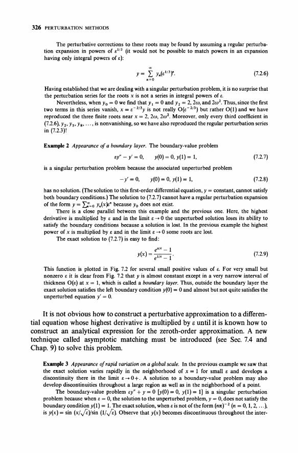
This function is plotted in Fig. 7.2 for several small positive values of E. For very small but nonzero E it is clear from Fig. 7.2 that y is almost constant except in a very narrow interval of thickness O(B) at x = I, which is called a boundary layer. Thus, outside the boundary layer the exact solution satisfies the left boundary condition y(O) = 0 and almost but not quite satisfies the unperturbed equation y' = O.

It is not obvious how to construct a perturbative approximation to a differen­tial equation whose highest derivative is multiplied by e until it is known how to construct an analytical expression for the zeroth-order approximation. A new technique called asymptotic matching must be introduced (see Sec. 7.4 and Chap. 9) to solve this problem.

Example 3 Appearance of rapid variation on a global scale. In the previous example we saw that the exact solution varies rapidly in the neighborhood of x = 1 for small E and develops a discontinuity there in the limit B --+ 0+. A solution to a boundary-value problem may also develop discontinuities throughout a large region as well as in the neighborhood of a point.

The boundary-value problem BY" + y = 0 [y(0) = 0, y(l) = 1] is a singular perturbation problem because when B = 0, the solution to the unperturbed problem, y = 0, does not satisfy the boundary condition y(l) = 1. The exact solution, when Bis not ofthe form (mtt2 (n = 0, 1,2, ... ~ is y(x) = sin (x/)6)/sin (1/)6). Observe that y(x) becomes discontinuous throughout the inter-

y

PERTURBATION SERIES 327

1.5 ~i --------------1

1.2

0.9

0.6

0.3

o 0.2 0.4 0.6

x

0.8

Boundary layer

~

1.0

Figure 7.2 A plot of y(x) = (~/, - 1 )j(e1/' - 1) (0 :;; x :;; 1) for e = 0.2, 0.1, 0.05, 0.025. When Bis small y(x) varies rapidly near x = 1; this localized region of rapid variation is called a boundary layer. When e is negative the boundary layer is at x = 0 instead of x = 1. This abrupt jump in the location of the boundary layer as e changes sign reflects the singular nature of the perturbation problem.

val 0 :;; x :;; 1 in the limit e ..... 0 + (see Fig. 7.3). When e = (n1t t 2, there is no solution to the boundary-value problem.

When the solution to a differential-equation perturbation problem varies rapidly on a global scale for small e, it is not obvious how to construct a leading­order perturbative approximation to the exact solution. The best procedure that has evolved is called WKB theory (see Chap. 10).

Example 4 Perturbation theory on an infinite interval. The initial-value problem

y" + (1 - ex)y = 0, y(O) = 1, itO) = 0, (7.2.10)

is a regular perturbation problem in e over the finite interval 0 :;; x :;; L In fact, the perturbation solution is just

y(x) = cos x + e(tx2 sin x + tx cos x - t sin x)

+ e2( -nx4 cos x + -isx3 sin x + 1f,x2 cos X - 1f,x sin x) + "', (7.2.11)

which converges for all x and e, with increasing rapidity as e ..... 0 + for fixed x.

328 PERTURBATION METHODS

4.0

3.0

2.0

LO

o

TI.O

-2.0

-3.0

-4.0

r-

V 1/

-

f-

f-

'--

I: = 0.00014 IF. = 0.005

~ ~

~ II

~r..f'.~ I

[IV 0.2 i\ 0.4 /

' ...... ..... l/

~

~ ~ ~ , I--'t--

f\. I/~

I \ I 1I I

0.6 i\ 0.8

/ / I. ,'-.....

o

~ ~

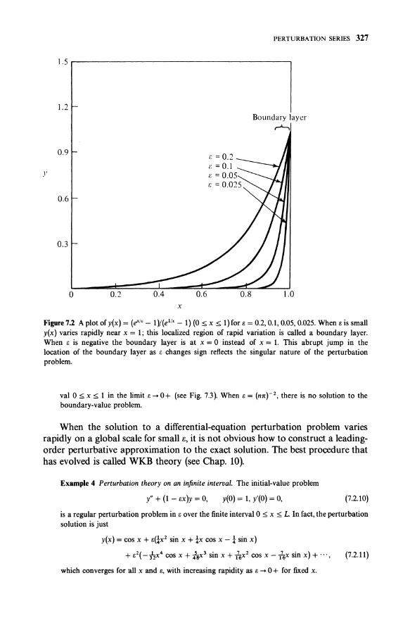
Figure 7.3 A plot of y(x) = [sin (xe-lIZ)]![sin (e- lIZ )] (0 ::; x ::; 1) fore = 0.005 and 0.00014. As e gets smaller the oscillations become more violent; as e -> 0 +, y(x) becomes discontinuous over the entire interval. The WKB approximation is a perturbative method commonly used to describe functions like y(x) which exhibit rapid variation on a global scale.

However, this same initial-value problem must be reclassified as a singular perturbation problem over the semi-infinite interval 0 ::; x < 00. While the exact solution does approach the solution to the unperturbed problem as e -> 0+ for fixed x, it does not do so uniformly for all x (see Fig. 7.4). The zeroth-order solution is bounded and oscillatory for all x. But when e > 0, local analysis of the exact solution for large x shows that it is a linear combination of exponentially increasing and decreasing functions (Prob. 7.20). This change in character of the solution occurs because it is certainly wrong to neglect ex compared with 1 when x is bigger than lie. In fact, a more careful argument shows that the term ex is not a small perturbation unless x «6- liZ (Prob. 7.20).

Example 4 shows that the interval itself can determine whether a perturbation problem is regular or singular. We examine more examples having this property in the next section on eigenvalue problems. The feature that is common to all such examples is that an nth-order perturbative approximation bears less and less resemblance to the exact solution as x increases.

For these sorts of problems Chap. 11 introduces new perturbative procedures called multiple-scale methods which substantially improve the rather poor predictions of ordinary perturbation theory. The particular problem in Example 4 is reconsidered in Prob. 11.13.

Example 5 Roots of a high-degree polynomial. When a perturbation problem is regular, the perturbation series is convergent and the exact solution is a smooth analytic function of e for

PERTURBATION SERIES 329

2.0

1.0

o I' 's '" If , '\' II u \\'''~_ u " " I " , '

-\.O

-2.0

-3.0

Frequencies differ whenx = 0(1:-1/2)

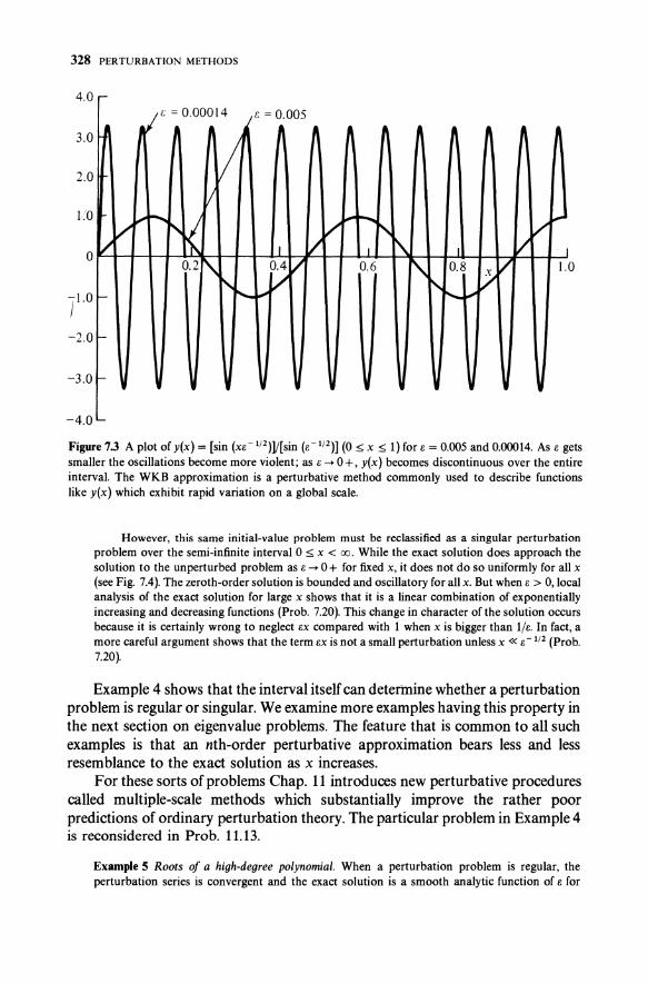
Figure 7.4 Exact solutions to the initial-value problem y" + (1 - 8X)Y = 0 [y(0) = I, y'(O) = 0] in (7.2.10) for 8 = 0 and 8 = iIT. Although this is a regular perturbation problem on the finite interval o ~ x ~ L, it is a singular perturbation problem on the infinite interval 0 ~ x ~ 00 because the perturbed solution (8 > 0) is not close to the unperturbed solution (8 = 0), no matter how small 8 is. When x = 0(8- 1/ 2 ) the frequencies begin to differ (the curves become phase shifted) and when x = 0(8- 1 ) the amplitudes differ (one curve remains finite while the other grows exponentially).

sufficiently small 8. However,just what is "sufficiently small" may vary enormously from problem to problem. A striking example by Wilkinson concerns the roots of the polynomial

20 n (x - k) + 8X 19 = x20 - (210 - 8)x19 + ... + 20! k~l

(7.2.12)

The perturbation ex 19 is regular, since no roots are lost in the limit 8 -+ 0; the roots of the unperturbed polynomial lie at I, 2, 3, ... , 20.

Let us now take 8 = 10- 9 so that the perturbation in the coefficient of X 19 is of relative magnitude 10- 9/210, or roughly 10- 11• For such a small regular perturbation one might expect the 20 roots to be only very slightly displaced from their 8 = 0 values. The actual displaced roots are given in Table 7.1. One is surprised to find that while some roots are relatively unchanged by the perturbation, others have paired into complex conjugates. The qualitative effect on the roots of varying 8 is shown in Figs. 7.5 and 7.6. In these plots the paths of the roots are traced as a function of 8. As I 8 I increases, the roots coalesce into pairs of complex conjugate roots. Evi­dently, a "small" perturbation is one for which lei < 10- 11 , while lei ~ 10- 10 is a "large" perturbation for at least some of the roots. Low-order regular perturbation theory may be used to understand this behavior (Probs. 7.22 and 7.23).

330 PERTURBATION METHODS

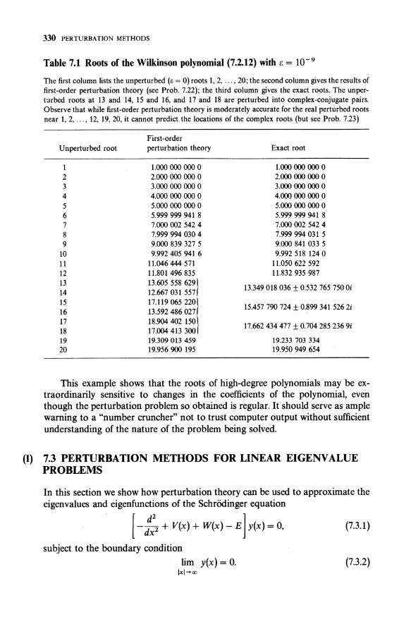
Table 7.1 Roots of the Wilkinson polynomial (7.2.12) with e = 10 - 9

The first column lists the unperturbed (8 = 0) roots 1, 2, ... , 20; the second column gives the results of first-order perturbation theory (see Prob. 7.22); the third column gives the exact roots. The unper­turbed roots at 13 and 14, 15 and 16, and 17 and 18 are perturbed into complex-conjugate pairs. Observe that while first-order perturbation theory is moderately accurate for the real perturbed roots near 1, 2, ... , 12, 19, 20, it cannot predict the locations of the complex roots (but see Prob. 7.23)

First-order Unperturbed root perturbation theory Exact root

1.000 000 000 0 1.000 000 000 0 2 2.000 000 000 0 2.000 000 000 0 3 3.000 000 000 0 3.000 000 000 0 4 4.000 000 000 0 4.000 000 000 0 5 5.000 000 000 0 5.000 000 000 0 6 5.999 999 941 8 5.999999941 8 7 7.000 002 542 4 7.000 002 542 4 8 7.999 994 030 4 7.999994031 5 9 9.000 839 327 5 9.000 841 033 5

10 9.992405 941 6 9.992 518 124 0 11 11.046444 571 11.050 622 592 12 11.801 496 835 11.832 935 987 13 13.605 558 6291 13.349018036 ± 0.532 765 750 Oi 14 12.667 031 557 15 17.1190652201 15.457790 724 ± 0.899 341 5262i 16 13.592 486 027 17 18.904 402 150 l 17.662434477 ± 0.704 285 236 9i 18 17.004 413 300 19 19.309 013 459 19.233 703 334 20 19.956900 195 19.950 949 654

This example shows that the roots of high-degree polynomials may be ex­traordinarily sensitive to changes in the coefficients of the polynomial, even though the perturbation problem so obtained is regular. It should serve as ample warning to a "number cruncher" not to trust computer output without sufficient understanding of the nature of the problem being solved.

(I) 7.3 PERTURBA nON METHODS FOR LINEAR EIGENVALUE PROBLEMS

In this section we show how perturbation theory can be used to approximate the eigenvalues and eigenfunctions of the SchrOdinger equation

[ -::2 + V(x) + W(x) - E] y(x) = 0, (7.3.1)

subject to the boundary condition

lim y(x) = o. (7.3.2) Ixl-+oo

1.0

0.8

0.6

0.4

0.2

Imx

010 9-

- S 7--6

- 5

-4

PERTURBATION SERIES 331

-10 9--s 7-

-6 -10 ·5 9-

- S -4 7-

- 6 ·3 - 5

- 4 -2

- 3

Rex o I b .,J r~;; ~-.J ;- ;-; I b .J

-0.2

-0.4

-0.6

11.0 12.0 13.0 14.0

-4

·5

-6 -7

s­-9

10-

-0.81- Complex-x plane

-1.0

15.0 16.0 17.0 18.0 19.0 20.0

- 3 - 2

-4

- 3 -5 -6

-4 ·7 ·s

-5 9· -6 -10

-7 -s

9--10

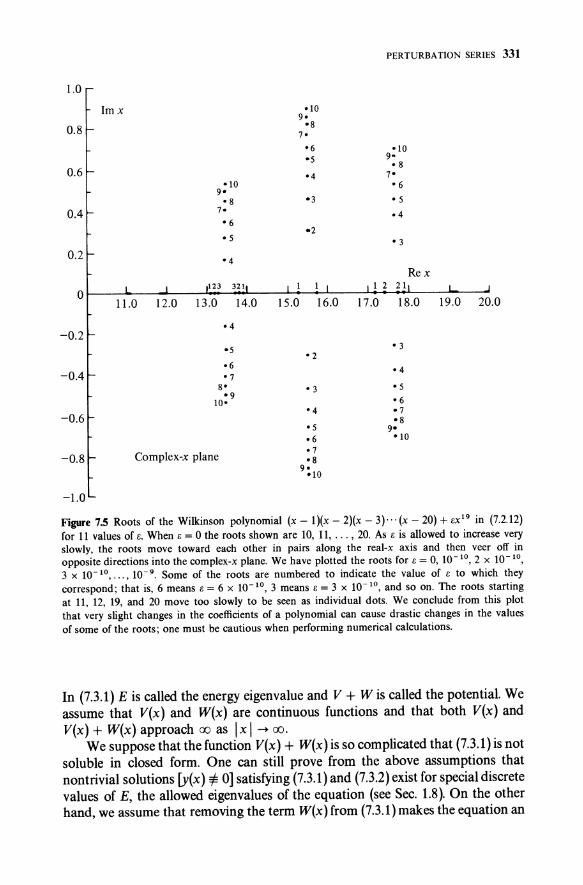
Figure 7.5 Roots of the Wilkinson polynomial (x - l)(x - 2)(x - 3)··· (x - 20) + BX 19 in (7.2.12) for 11 values of B. When B = 0 the roots shown are 10, 11, ... , 20. As B is allowed to increase very slowly, the roots move toward each other in pairs along the real-x axis and then veer off in opposite directions into the complex-x plane. We have plotted the roots for B = 0, 10- 1°,2 X 10- 1°, 3 X 10- 1°, ... , 10- 9. Some of the roots are numbered to indicate the value of B to which they correspond; that is, 6 means B = 6 X 10- 10, 3 means B = 3 X 10- 1°, and so on. The roots starting at 11, 12, 19, and 20 move too slowly to be seen as individual dots. We conclude from this plot that very slight changes in the coefficients of a polynomial can cause drastic changes in the values of some of the roots; one must be cautious when performing numerical calculations.

In (7.3.1) E is called the energy eigenvalue and V + W is called the potential. We assume that V(x) and W(x) are continuous functions and that both V(x) and V(x) + W(x) approach 00 as Ixl-+oo.

We suppose that the function V(x) + W(x) is so complicated that (7.3.1) is not soluble in closed form. One can still prove from the above assumptions that nontrivial solutions [y(x) =1= 0] satisfying (7.3.1) and (7.3.2) exist for special discrete values of E, the allowed eigenvalues of the equation (see Sec. 1.8). On the other hand, we assume that removing the term W(x) from (7.3.1) makes the equation an

332 PERTURBATION METHODS

1.0 I

Imx -10 9-

O.SI- -s -10 7-9-- S -6

7- -s 0.61- - 6

-5 -4

- 4 -3 0041-

-10 - 3 -2 9-

-s 0.2 t- - 7

-10 - 2

01 I L..:: • 11.0 12.0 13.0 14.0 15.0 16.0 17.0 IS.O 19.0 20.0

- 10 - 2 -0.2r - 7

-2 -s 9-

- 3 -10 -0041--

-4 -3

- S -4 -0.61- - 6 -s

- 7 s- -6 - 9 -7

-O.S~ 10- -s

9--10

I -\.O

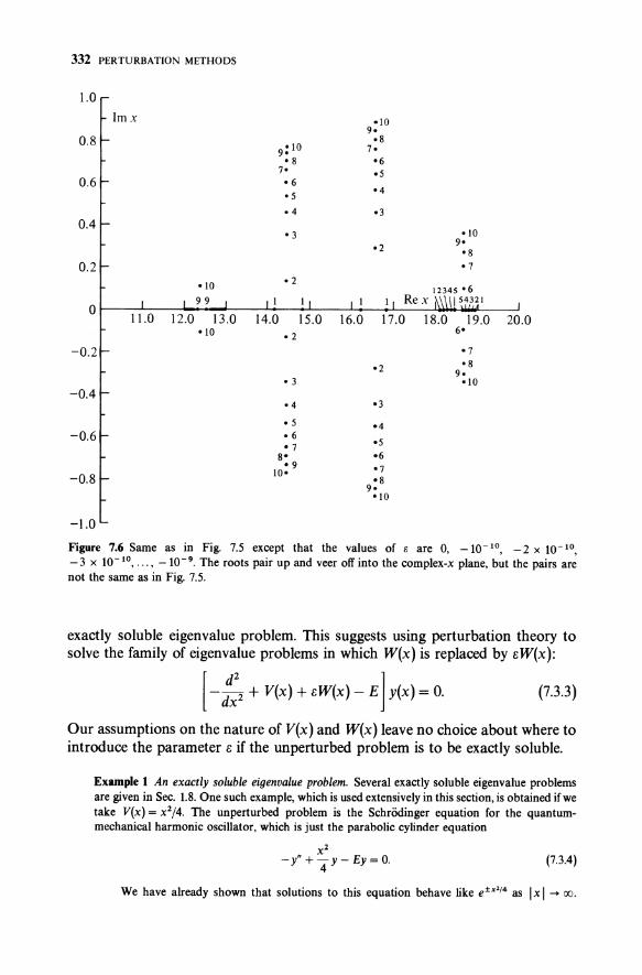
Figure 7.6 Same as in Fig. 7.5 except that the values of e are 0, -10- 10, - 2 x 10- 10,

-3 X 10- 1°, ... , _10- 9• The roots pair up and veer off into the complex-x plane, but the pairs are not the same as in Fig. 7.5.

exactly soluble eigenvalue problem. This suggests using perturbation theory to solve the family of eigenvalue problems in which W(x) is replaced by 6 W(x):

[ -::2 + V(x) + 6W(X) - E] y(x) = O. (7.3.3)

Our assumptions on the nature of V(x) and W(x) leave no choice about where to introduce the parameter 6 if the unperturbed problem is to be exactly soluble.

Example 1 An exactly soluble eigenvalue problem. Several exactly soluble eigenvalue problems are given in Sec. 1.8. One such example, which is used extensively in this section, is obtained if we take V(x) = x2/4. The unperturbed problem is the Schrooinger equation for the quantum­mechanical harmonic oscillator, which is just the parabolic cylinder equation

" x2 - Y + 4 y - Ey = o. (7.3.4)

We have already shown that solutions to this equation behave like e±x1 /4 as I x I .... 00.

PERTURBATION SERIES 333

There is a discrete set of values of E for which a solution that behaves like e - x'/4 as x ---+ 00 also behaves like e- x '/4 as x ---+ - 00 (see Example 4 of Sec. 3.5 and Example 9 of Sec. 3.8). These values of E are

E = n + 1, n = 0, 1, 2, ... , (7.3.5)

and the associated eigenfunctions are parabolic cylinder functions

y.(x) = D.(x) = e- x '/4 He. (x), (7.3.6)

where He. (x) is the Hermite polynomial of degree n: Heo (x) = 1, He! (x) = x, He2 (x) = x2 - 1, ....

In general, once an eigenvalue Eo and an eigenfunction Yo(x} of the unper­turbed problem

l-::2 + V(X}-Eojyo(X}=O (7.3.7)

have been found, we may seek a perturbative solution to (7.3.3) of the form

00

E = L EnEf', (7.3.8) n=O

00

y(x} = L yix )en. (7.3.9) n=O

Substituting (7.3.8) and (7.3.9) into (7.3.3) and comparing powers of e gives the following sequence of equations:

l d2 j n --d 2 + V(x}-Eo Yn(x} = -WYn-1(X} + .L EjYn-Ax},

x J=1

n = 1,2,3, ... , (7.3.1O)

whose solutions must satisfy the boundary conditions

lim Yn(x} = 0, n = 1,2,3, .... (7.3.11) Ixl-+oo

Equation (7.3.1O) is linear and inhomogeneous. The associated homogeneous equation is just the unperturbed problem and thus is soluble by assumption. However, technically speaking, only one of the two linearly independent solutions of the unperturbed problem (the one that satisfies the boundary conditions) is assumed known. Therefore, we proceed by the method of reduction of order (see Sec. 1.4); to wit, we substitute

Yn(x} = Yo(x}Fn(x}, {7.3.12}

where F o(x} = 1, into (7.3.10). Simplifying the result using (7.3.7) and multiplying by the integrating factor Yo(x} gives

:x[y5(X}F~(X}]=YMx} lW{X}Fn- 1(X}- it1 EjFn-AX}j. {7.3.13}

334 PERTURBATION METHODS

If we integrate this equation from - 00 to 00 and use y~(x )F~(x) = Yo(x)y~(x) - YO(x)Yn(x) -+ 0 as I x I -+ 00, we obtain the formula for the coefficient En:

E ~ r. Yo(x l[ W(xly.-. (xl - :~ EjY._ i(x l] dx

n 00 ' f y~(x) dx -00

n = 1,2,3, ... , (7.3.14 )

from which we have eliminated all reference to Fn(x). [The sum on the right side of (7.3.l4) is defined to be 0 when n = 1.]

Integrating (7.3.13) twice gives the formula for Yn(x):

"dt t [ n ] Yn(x)=yO(x) f -Y-()f dsyo(s) W(s)Yn-1(S)-.L EjYn_j(s) ,

a Yo t - 00 J= 1

n = 1,2, 3, .... (7.3.15)

Observe that in (7.3.15) a is an arbitrary number at which we choose to impose Yn(a) = O. This means we have fixed the overall normalization of y(x) so that y(a) = Yo(a) [assuming that Yo(a) + 0]. If Yo(t) vanishes between a and x, the integral in (7.3.15) seems formally divergent; however, Yn(x) satisfies a differential equation (7.3.10) which has no finite singular points. Thus, it is possible to define Yn(x) everywhere as a finite expression (see Prob. 7.24).

Equations (7.3.14) and (7.3.15) together constitute an iterative procedure for calculating the coefficients in the perturbation series for E and y(x). Once the coefficients Eo, E1, ... , En- b Yo, Yb ..• , Yn-1 are known, (7.3.14) gives En, and once En has been calculated (7.3.15) gives Yn. The remaining question is whether or not these perturbation series are convergent.

Example 2 A regular perturbative eigenvalue problem. Let V(x) = x 2/4 and W(x) = x. It may be shown (Prob. 7.25) that the perturbation series for y(x) is convergent for aile and that the series for E has vanishing terms of order F!' for n ~ 3. This is a regular perturbation problem.

Example 3 A singular perturbative eigenvalue problem. It may be shown (Prob. 7.26) that if V(x) = x 2/4 and W(x) = x4/4, then the perturbation series for the smallest eigenvalue for positive sis

E(e) -1 + ie - ¥e 2 + We3 + ... , e~O+. (7.3.16)

The terms in this series appear to be getting larger and suggest that this series may be divergent for all Il ¥- O. Indeed, (7.3.16) diverges for all e because the nth term satisfies E.­- ( - 3)"nn + !)j6/7t3/2 (n ~ (0). (This is a nontrivial result that we do not explain here.)

The divergence of the perturbation series in Example 3 indicates that the perturbation problem is singular. A simple way to observe the singular behavior is to compare e- x'/4, the controlling factor of the large-x behavior of the unperturbed (e = 0) solution, with e- x1';;'/6, the controlling factor of the large-x behavior for Il '" O. There is an abrupt change in the nature of the solution when we pass to the limit (e ~ 0 + ). This phenomenon occurs because the perturbing term ex4/4 is not small compared with x 2/4 when x is large.

PERTURBATION SERIES 335

If the functions V(x) and W(x) in Example 3 were interchanged, then the resulting eigenvalue problem would be a regular perturbation problem because ox 2 is a small perturbation of X4 for alllxl<oo. However, the unperturbed problem, (-d 2/dx 2 +x4/4-Eo)Yo(x)=O, is not soluble in closed form. Thus, it would not be possible to use (7.3.14) and (7.3.15) to compute the coefficients in the perturbation series analytically.

Also note that if the boundary conditions in Example 3 were given at x = ± A, A < 00, then the perturbation theory would be regular. This is because here ox4 is a small perturbation of x2 .

However, it is much more difficult to solve the unperturbed problem on a finite interval. Thus, one is forced to accept a solution to Example 3 in the form of a divergent series.

Fortunately, this series is one of many that may be summed by Pade theory to give a finite and unique result (see Sec. 8.3).

Example 4 Another regular perturbation problem. When V = x 2/4 and W = I x I the perturba­tion problem is regular. But unlike the problem in Example 2, this perturbation series is not convergent for all 0; the series in (7.3.8) and (7.3.9) have finite radii of convergence. The significance of the finite radius of convergence is discussed in Sec. 7.5.

(D) 7.4 ASYMPTOTIC MATCHING

The purpose of this section is to introduce the notion of matched asymptotic expansions. Asymptotic matching is an important perturbative method which is used often in both boundary-layer theory (Chap. 9) and WKB theory (Chap. 10) to determine analytically the approximate global properties of the solution to a differential equation. Asymptotic matching is usually used to determine a uniform approximation to the solution of a differential equation and to find other global properties of differential equations such as eigenvalues. Asymptotic matching may also be used to develop approximations to integrals.

The principle of asymptotic matching is simple. The interval on which a boundary-value problem is posed is broken into a sequence of two or more overlapping subintervals. Then, on each subinterval perturbation theory is used to obtain an asymptotic approximation to the solution of the differential equation valid on that interval. Finally, the matching is done by requiring that the asymptot­ic approximations have the same functional form on the overlap of every pair of intervals. This gives a sequence of asymptotic approximations to the solution of the differential equation; by construction, each approximation satisfies all the boundary conditions given at various points on the interval. Thus, the end result is an approximate solution to a boundary-value problem valid over the entire interval.

Asymptotic matching bears a slight resemblance to an elementary technique for solving boundary-value problems called patching. Patching is helpful when the differential equation can be solved in closed form. Here is a simple example:

Example 1 Patching. The method of patching may be used to solve the boundary-value problem y" - y = e -Ixl [y( ± 00 ) = 0]. There are two regions to consider. When x :0; 0, the most general solution which satisfies the boundary condition y( - 00 ) = 0 is

y(x) = aeX + !xex, (7.4.1)