PERSPECTIVE Midpoint attractors and species richness...

IDEA AND

PERSPECT IVE Midpoint attractors and species richness: Modelling the

interaction between environmental drivers and geometric

constraints

Robert K. Colwell,1,2,3* Nicholas J.

Gotelli,4 Louise A. Ashton,5,6 Jan

Beck,3,7 Gunnar Brehm,8 Tom M.

Fayle,9,10,11 Konrad Fiedler,12

Matthew L. Forister,13 Michael

Kessler,14 Roger L. Kitching,5 Petr

Klimes,9 J€urgen Kluge,15 John T.

Longino,16 Sarah C. Maunsell,5

Christy M. McCain,3,17 Jimmy

Moses,18,19 Sarah Noben,14

Katerina Sam,9 Legi Sam,5,9 Arthur

M. Shapiro,20 Xiangping Wang21

and Vojtech Novotny9,18

Abstract

We introduce a novel framework for conceptualising, quantifying and unifying discordant patternsof species richness along geographical gradients. While not itself explicitly mechanistic, thisapproach offers a path towards understanding mechanisms. In this study, we focused on thediverse patterns of species richness on mountainsides. We conjectured that elevational range mid-points of species may be drawn towards a single midpoint attractor – a unimodal gradient of envi-ronmental favourability. The midpoint attractor interacts with geometric constraints imposed bysea level and the mountaintop to produce taxon-specific patterns of species richness. We devel-oped a Bayesian simulation model to estimate the location and strength of the midpoint attractorfrom species occurrence data sampled along mountainsides. We also constructed midpoint predic-tor models to test whether environmental variables could directly account for the observed pat-terns of species range midpoints. We challenged these models with 16 elevational data sets,comprising 4500 species of insects, vertebrates and plants. The midpoint predictor models gener-ally failed to predict the pattern of species midpoints. In contrast, the midpoint attractor modelclosely reproduced empirical spatial patterns of species richness and range midpoints. Gradientsof environmental favourability, subject to geometric constraints, may parsimoniously account forelevational and other patterns of species richness.

Keywords

Bayesian model, Biogeography, elevational gradients, geometric constraints, mid-domain effect,midpoint predictor model, stochastic model, truncated niche.

Ecology Letters (2016) 19: 1009–1022

INTRODUCTION

The search for a unified mechanistic understanding ofrepeated, global and regional patterns of species richness haslong been frustrated by taxonomic and geographical

idiosyncrasies, lack of reliable climatic data on appropriatespatial scales, and reliance on case studies built from statisti-cal correlation and post hoc conjecture. We offer no cures forthese many ills, but instead, propose a novel conceptualapproach. While not itself mechanistic, by unifying and

1Department of Ecology and Evolutionary Biology, University of Connecticut,

Storrs, CT 06269, USA2Departmento de Ecologia, Universidade Federal de Goi�as, CP 131, Goiania,

GO 74.001-970, Brasil3University of Colorado Museum of Natural History, Boulder, CO 80309, USA4Department of Biology, University of Vermont, Burlington, VT 05405, USA5Environmental Futures Research Institute, Griffith University, Nathan, Qld

4111, Australia6Life Sciences Department, Natural History Museum, South Kensington,

London, SW7 5BD, UK7Department of Environmental Science (Biogeography), University of Basel,

Basel, Switzerland8Phyletisches Museum, Friedrich-Schiller Universit€at, Jena 07743, Germany9Institute of Entomology, Biology Centre of the Czech Academy of Sciences

and Faculty of Science, University of South Bohemia, Brani�sovsk�a 31, 370 05�Cesk�e Bud�ejovice, Czech Republic10Forest Ecology and Conservation Group, Imperial College London, Silwood

Park Campus, Buckhurst Road, Ascot, Berkshire, SL5 7PY, UK

11Institute for Tropical Biology and Conservation, Universiti Malaysia Sabah,

88400 Kota Kinabalu, Sabah, Malaysia12Department of Botany & Biodiversity Research, University of Vienna,

Rennweg 14, 1030 Vienna, Austria13Program in Ecology, Evolution, and Conservation Biology, Department of

Biology, University of Nevada, Reno, NV 89557, USA14Institute of Systematic Botany, University of Zurich, 8008 Zurich, Switzerland15Department of Geography, University of Marburg, 35032 Marburg, Germany16Department of Biology, University of Utah, Salt Lake City, UT 84112, USA17Department of Ecology and Evolutionary Biology, University of Colorado,

Boulder, CO 80309, USA18New Guinea Binatang Research Center, P.O. Box 604, Madang, Papua New

Guinea19School of Natural and Physical Sciences, University of Papua New Guinea,

P.O. Box 320, National Capital District, Papua New Guinea20Center for Population Biology, University of California, Davis, CA 95616,

USA21College of Forestry, Beijing Forestry University, Beijing 100083, China

*Correspondence: E-mail: [email protected]

© 2016 John Wiley & Sons Ltd/CNRS

Ecology Letters, (2016) 19: 1009–1022 doi: 10.1111/ele.12640

quantifying discordant patterns of species richness, this frame-work offers a path towards understanding mechanism. Wedevelop and illustrate this approach for terrestrial, elevationalgradients. However, the framework and statistical model arequite general, could easily be applied to other habitats, andcould be extended from one-dimensional to two- or eventhree-dimensional spatial domains.Along any continental latitudinal transect, species richness

for most higher taxa peaks in the tropics, where mean annualtemperature is the highest and annual variability in tempera-ture is lowest (Wright et al. 2009; Chan et al. 2016). Regard-less of latitude, temperature on most mountainsides declinessteadily with elevation, driven by adiabatic cooling, so thatthe warmest temperatures usually prevail at the bottom of ele-vational gradients (Ahrens 2013; Fan & van den Dool 2008).Net primary productivity (NPP), although crucially dependenton precipitation, is strongly driven by temperature. Thus, ifradiant energy or NPP are fundamentally responsible for thelatitudinal richness pattern, as many ecologists suggest (Currieet al. 2004; Allen et al. 2007), species richness for higher taxaalong elevational transects in humid climates should beexpected to peak at the lowest elevations.However, in a review of hundreds of published examples,

Rahbek (1995, 2005) showed that species richness usually doesnot peak at the bottom of elevational gradients. For the pre-ponderance (70%) of studies that encompassed complete ele-vational gradients and accounted for sampling effects, speciesrichness peaked, instead, at intermediate elevations. Decliningrichness with elevation was the second most-common pattern,but was found in < 20% of studies (Rahbek 2005). Amongother things, these meta-analyses imply that, for most terres-trial taxa, local species richness peaks at intermediate tropicalelevations, rather than in the tropical lowlands.Many explanations have been proposed for mid-elevation

richness peaks, and surely no single factor is responsible. Forsome clades, intermediate climatic conditions at these eleva-tions may be more suitable for survival and reproduction:

lower elevations may be too hot or too dry (McCain 2007)and higher elevations too cold, too wet or too cloudy (Long-ino et al. 2014). A history of speciation (or more precisely,net diversification) within a clade that is constrained by itsheritable environmental tolerances to a specific range of eleva-tions, can lead to a build-up of species at intermediate eleva-tions (Graham et al. 2014; Wu et al. 2014). In the tropics, ahistory of mountaintop extinctions during glacial minima andsea level extinctions during glacial maxima could also produceor enhance mid-elevation richness peaks (Colwell & Rangel2010). Spatially structured dispersal within an elevationaldomain, such as source-sink dynamics (Grytnes 2003; Grytneset al. 2008) or ecotonal mixing (Lomolino 2001), could alsolead to peaks of species richness at intermediate elevations.

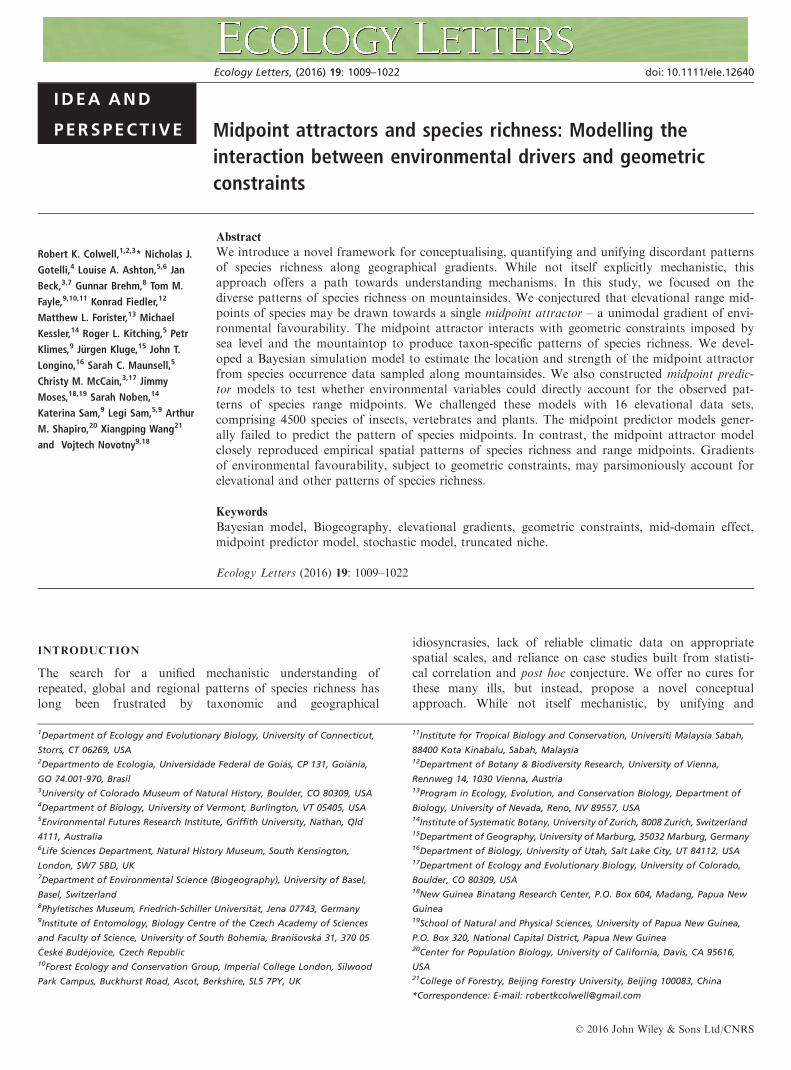
Geometric constraints

In addition to these ecological and historical explanations,Colwell & Hurtt (1994) showed, with a simple stochasticmodel, that a mid-elevation richness peak might be expectedeven in the absence of climatic drivers or historical forces.In their model, a mid-elevation richness peak arises from thetendency of larger species ranges to overlap more at mid-ele-vations than at high or low elevations, when they are geo-metrically constrained by the hard boundaries (sea level andthe mountaintop) of an elevational domain. Figure 1a offersa physical analogy (a pencil-box) for this phenomenon,which later became known as the mid-domain effect (Colwell& Lees 2000) or MDE, because, in a simple 1-dimensionaldomain, the expected distribution of species richness underthis model is exactly symmetrical about the centre of thedomain. Geometric constraints have been generalised toother bounded spatial (Storch et al. 2006) and non-spatial(Letten et al. 2013) domains at the assemblage level, as wellas to studies of home ranges (Prevedello et al. 2013) and themovement of individuals within a population (Tiwari et al.2005).

E(n)E(n)

(a) (b)

Figure 1 Geometric constraint models. (a) The classic geometric constraint model illustrated by a physical analogy: a set of pencils (species), some shorter

and some longer (narrower and wider elevational ranges), stored in a schoolchild’s old-fashioned pencil-box (the bounded elevational domain) (Colwell

et al. 2004). If the box is shaken end to end, horizontally, so that the position of each pencil is randomised, the expected number E(n) of pencils that

overlap (species richness) near the middle of the box is inevitably greater than the number that overlap nearer the ends of the box, a pattern that is

symmetric around the centre of the box. But the constraint does not act uniformly on the pencils as the box is shaken: the shorter pencil stubs move more

widely and freely than the longer pencils. By analogy, the distribution of small-ranged species is less constrained by geometry than the distribution of large-

ranged species (Colwell & Lees 2000; Dunn et al. 2007). (b) A physical analogy for the midpoint attractor model. Suppose that each pencil has a steel ball

bearing embedded at its midpoint (blue circles). A magnetic field, the attractor, is applied across the pencil box (green). As the box is shaken end to end,

the pencils tend to collect near the attractor, as their midpoint ball bearings are drawn towards the magnet. If the attractor is located near one end of the

box, as illustrated, the expected number of pencils E(n) that stack up at any location along the length of the pencil box is asymmetric. However, because

the midpoints of the longer pencils cannot align with the magnet (since longer pencils abut the end of the box), the peak of E(n) does not coincide with the

centre of the attractor. Thus E(n) is influenced jointly by the attractor (the magnet) and the constraint (the limits of the pencil box). The pattern of E(n) is

narrow when the attractor is strong, broad when the attractor is weak.


1010 R. K. Colwell et al. Idea and Perspective

Early studies treated geometric constraints as a stand-alonehypothesis, subject to falsification if it failed to fully explainpatterns of richness (see Colwell et al. 2004, 2005), or strictlyas an alternative hypothesis to environmental explanations(Currie & Kerr 2008). But this either/or perspective misses thepoint that constraints and drivers do not operate indepen-dently, but instead interact. It has proven challenging to inte-grate geometric constraints with environmental and historicalexplanations for patterns of species richness. We review thehistory of these efforts in Appendix 2, Supplemental Introduc-tion.

A Bayesian midpoint attractor model

The likelihood that several different mechanisms contribute toelevational richness peaks calls for a conceptually andmethodologically unifying approach to these patterns at a dif-ferent level. We introduce the idea that species elevationalranges, which underlie elevational richness gradients, can betreated and modelled as if responding, independently, to a sin-gle environmental attractor that operates within the geometricconstraints of an elevational domain and is specific to ataxon-based assemblage. We develop this approach as a simu-lation model, apply it to a diverse group of data sets, andthen discuss it from the broader perspective of biogeographi-cal gradients.We take a novel approach to integrating environment with

geometric constraints over elevational gradients. Inspired byWang & Fang’s (2012) evidence that large- and small-rangedspecies respond similarly to environmental drivers and byRangel & Diniz-Filho’s (2005) mechanistic model, we postu-late the presence of an underlying unimodal ‘favourability’gradient, specific to each elevational transect and to eachtaxon or functional group.We modelled the simplest possible pattern of environmental

favourability – a unimodal peak – on the simplest possibledomain – the unit line. The model is general, but in thisstudy, we assume that the one-dimensional unit domain repre-sents an elevational transect from low elevation (sea level, forall our data sets) to the highest habitable point on a mountainmassif. Somewhere along this elevational domain lies a uni-modal midpoint attractor, specific to the locality and taxon,representing a gradient of ‘attraction’ for species range mid-points. A continuous function describes the relative strengthof the attractor at every point within the domain (Fig. 2).We model the midpoint attractor as a normal (Gaussian)

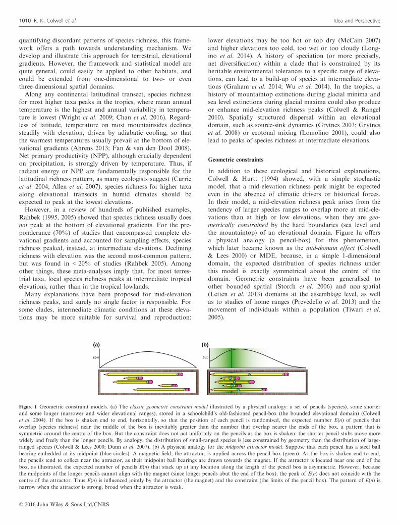
probability density function N(A, B) with two parameters: itsmean location A (0 < A < 1) on the unit-line domain, and itsstandard deviation B (0 < B < 1) around the attractor, aninverse measure of attractor strength (Fig. 2). Because theunit domain is bounded at 0 and 1, A and B determine notonly the location and shape of the attractor, but also jointlydefine the upper and lower bounds of the attractor distribu-tion, which is truncated at the domain limits (Fig. 2). To sim-ulate a bounded elevational richness pattern driven by themidpoint attractor, we place the empirical elevational ranges(transformed to unit-line equivalents) on the domain stochas-tically, sampling their midpoints from the modelled attractorprobability density function (which we will henceforth call,

simply, the attractor). Figure 1b updates the pencil-box anal-ogy for the classic MDE by adding an off-centre attractor forpencil midpoints.We developed a Bayesian model to estimate the optimum

shape and position of the midpoint attractor for a particulartaxon on a particular elevational gradient. The model aims toexplain the empirical distribution of species elevational ranges(as indexed by their elevational midpoints), and thus toaccount for empirical patterns of richness on mountainsides,under geometric constraints. With a centred Gaussian distri-bution as the starting point, the model employs a simpleGibbs sampler (Gelman et al. 2013) to find the posterior dis-tributions of parameter values for the attractor (its location,A, and strength, B), that are most probable (P(model | data)),given the observed elevational pattern of species richness andthe empirical range size frequency distribution (RSFD).The midpoint attractor model does not incorporate any

environmental data into the estimation of these parameters. Itmakes no assumptions or a priori hypotheses about whichenvironmental or biotic factors might be driving the attractorand the favourability gradient it represents. Instead, once awell-fitting attractor model has been identified using thisapproach, we subsequently attempt to interpret the attractorstatistically in terms of empirically measured environmentalvariables.Although the midpoint attractor model maximises

P(model | data), most previous attempts to interpret richnesspatterns have, instead, been conducted in a traditional, fre-quentist framework, estimating the probability of the data(observed richness), given a specified multivariate statisticalmodel (P(data | model)). The statistical model usually takesthe form of a regression of species richness on environmentalvariables, with (Longino & Colwell 2011) or without (Haw-kins et al. 2003) a predictor variable for geometric constraints.To compare the results from our Bayesian analyses with thesetraditional, correlative analyses, we carried out multipleregressions of species richness over elevational gradients, as a

A

B

mean

SDBSD

Mid

poin

t pro

babi

lity

dens

ity

Domain0 1

Doubly-truncated Normal distribution

Figure 2 The midpoint attractor modelled with a doubly truncated

Gaussian probability density function with mean A and standard

deviation B. Parameter A controls the position of the attractor on the

gradient. Parameter B controls the strength of the attractor (small B = a

strong attractor, large B = a weak attractor).


Idea and Perspective Midpoint attractors and species richness 1011

direct function of the same environmental variables that weused to interpret the attractors.

Midpoint predictor models

In addition to the midpoint attractor model, we built twoalternative, stochastic, midpoint predictor models – one withand one without geometric constraints – that directly assessedenvironmental variables as predictors of midpoint density (notspecies richness) over the elevational gradient. In these mod-els, as in the midpoint attractor model, each empirical rangemidpoint is placed on the domain stochastically. However,range placement is not driven by a hypothetical attractor, asit is in the Bayesian midpoint attractor model. Instead, ateach point in the domain, the probability of midpoint place-ment is directly and linearly proportional to the value of asingle, measured, environmental variable (e.g. temperature orprecipitation), regardless of the elevational pattern of the vari-able. Although the midpoint attractor model seeks an optimallocation and optimal strength for a hypothetical attractor, themidpoint predictor models assess the fit of the empirical mid-point data to a probability distribution directly defined by ameasured environmental variable. This approach is somewhatakin to the models of Storch et al. (2006) and Rahbek et al.(2007), but contrasts with the traditional MDE model, inwhich the probability of midpoint occurrence is constantacross the domain.

Application of the models

We applied the midpoint attractor model and the two mid-point predictor models to 16 high-quality data sets thatrecorded the elevational distribution of more than 4500 spe-cies of ferns, insects, mammals or birds in globally distributedlocalities, mostly in the tropics (Table S1, Appendix 1). As wewill demonstrate, with or without geometric constraints, themidpoint predictor models generally provide a poor fit to theobserved pattern of range midpoints. In contrast, the Bayesianmidpoint attractor model simulations consistently produce agood fit to both species richness and midpoint distributions ofempirical data sets.

MATERIALS AND METHODS

Empirical data sets and data representation

We applied the midpoint attractor model and the two mid-point predictor models to the 16 data sets detailed in Table S1(Appendix 1). Three groups of data sets included multiple taxastudied on the same gradients: northern Costa Rica, Mt. Wil-helm in Papua New Guinea and the Border Ranges in Aus-tralia. To label the individual data sets, we preface the nameof the taxonomic group with the name of the geographicallocation of the gradient (e.g. ‘New Guinean ants’, ‘CostaRican ferns’, etc.). The biogeographical data from these stud-ies consist of species occurrences recorded at a variable num-ber of sampling elevations (5–70 elevations, median = 8)along each gradient. Each data set also included measure-ments for two or more environmental factors along the

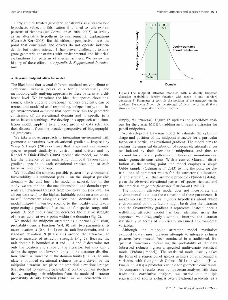
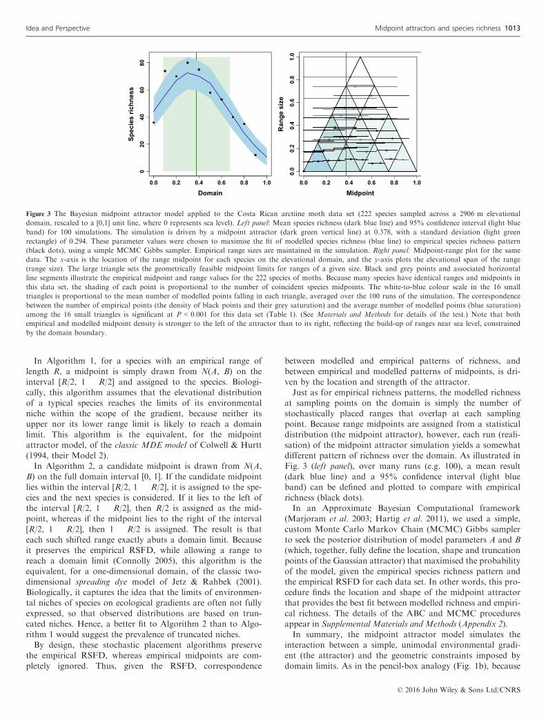
gradient (Table S1, Appendix 1). We rescaled each elevationaldomain to the [0, 1] unit line. Within this domain, we stan-dardised sampling points and converted species occurrencerecords into an estimated elevational range and midpoint foreach species, following data preparation protocols detailed inSupplemental Materials and Methods (Appendix 2). Each dataset was represented in two ways: A midpoint-range plot (Col-well & Hurtt 1994), with range size as the ordinate and rangemidpoint as the abscissa for each range in a data set (Fig. 3,right panel, grey-scale dots and horizontal line segments), anda corresponding species richness plot, showing the number ofoverlapping ranges at each of a sequence of sampling loca-tions (elevations) spanning the domain (Fig. 3, left panel,black dots).

The Bayesian midpoint attractor model

As outlined in the Introduction, we modelled the midpointattractor as a Gaussian probability density function N(A, B)with two parameters: its mean location A (0 < A < 1) on theunit-line domain, and its standard deviation B (0 < B < 1)around the attractor (Fig. 2). Because a Gaussian distributionextends from negative to positive infinity, the attractor distri-bution is truncated at the lower (0) and upper (1) bounds ofthe domain.The choice of a unimodal midpoint attractor distribution

was based on the empirical prevalence in the published litera-ture of unimodal peaks of species richness (Rahbek 2005),which in turn suggest unimodal midpoint patterns. Our choiceof a doubly truncated Gaussian distribution to represent theattractor, rather than a probability distribution that declinesto zero at the domain limits (e.g. the beta distribution), wasbased on biological grounds: many species are regularly pre-sent at either sea level or mountaintop, their realised distribu-tions directly abutting a domain limit. Such geographicaldistributions suggest that these species could readily toleratemore extreme conditions than those at domain limits, on aparticular elevational gradient. For example species living atsea level on a mid-latitude elevational gradient might well tol-erate even warmer temperatures at a lower latitude. Funda-mental niches may fail to be fully expressed for many reasons,but we suggest that elevational domain limits may oftenimpose environmental niche truncation (Colwell & Rangel2009; Feeley & Silman 2010).To model the expected pattern of species richness under the

influence of the attractor, each of the empirical ranges in adata set is placed on the domain stochastically, withoutreplacement, with its midpoint drawn at random from a pro-posed attractor distribution N(A, B). To enforce the geometricconstraint (Fig. 3, right panel) and maintain the empiricalRSFD, the midpoint is sampled from this distribution onlyover the interval of feasible midpoints, given the size of eachrange, such that the range does not extend beyond either thelower or upper domain limit (Colwell & Lees 2000). For arange of length R, this means that the midpoint must lie in theinterval [R/2, 1 � R/2]. For these stochastic range simulations,we explored two alternative algorithms for placing rangeswithin the domain, within this constraint. The two algorithmsdiffer only in how the placement constraint is achieved.



In Algorithm 1, for a species with an empirical range oflength R, a midpoint is simply drawn from N(A, B) on theinterval [R/2, 1 � R/2] and assigned to the species. Biologi-cally, this algorithm assumes that the elevational distributionof a typical species reaches the limits of its environmentalniche within the scope of the gradient, because neither itsupper nor its lower range limit is likely to reach a domainlimit. This algorithm is the equivalent, for the midpointattractor model, of the classic MDE model of Colwell & Hurtt(1994, their Model 2).In Algorithm 2, a candidate midpoint is drawn from N(A,

B) on the full domain interval [0, 1]. If the candidate midpointlies within the interval [R/2, 1 � R/2], it is assigned to the spe-cies and the next species is considered. If it lies to the left ofthe interval [R/2, 1 � R/2], then R/2 is assigned as the mid-point, whereas if the midpoint lies to the right of the interval[R/2, 1 � R/2], then 1 � R/2 is assigned. The result is thateach such shifted range exactly abuts a domain limit. Becauseit preserves the empirical RSFD, while allowing a range toreach a domain limit (Connolly 2005), this algorithm is theequivalent, for a one-dimensional domain, of the classic two-dimensional spreading dye model of Jetz & Rahbek (2001).Biologically, it captures the idea that the limits of environmen-tal niches of species on ecological gradients are often not fullyexpressed, so that observed distributions are based on trun-cated niches. Hence, a better fit to Algorithm 2 than to Algo-rithm 1 would suggest the prevalence of truncated niches.By design, these stochastic placement algorithms preserve

the empirical RSFD, whereas empirical midpoints are com-pletely ignored. Thus, given the RSFD, correspondence

between modelled and empirical patterns of richness, andbetween empirical and modelled patterns of midpoints, is dri-ven by the location and strength of the attractor.Just as for empirical richness patterns, the modelled richness

at sampling points on the domain is simply the number ofstochastically placed ranges that overlap at each samplingpoint. Because range midpoints are assigned from a statisticaldistribution (the midpoint attractor), however, each run (reali-sation) of the midpoint attractor simulation yields a somewhatdifferent pattern of richness over the domain. As illustrated inFig. 3 (left panel), over many runs (e.g. 100), a mean result(dark blue line) and a 95% confidence interval (light blueband) can be defined and plotted to compare with empiricalrichness (black dots).In an Approximate Bayesian Computational framework

(Marjoram et al. 2003; Hartig et al. 2011), we used a simple,custom Monte Carlo Markov Chain (MCMC) Gibbs samplerto seek the posterior distribution of model parameters A and B(which, together, fully define the location, shape and truncationpoints of the Gaussian attractor) that maximised the probabilityof the model, given the empirical species richness pattern andthe empirical RSFD for each data set. In other words, this pro-cedure finds the location and shape of the midpoint attractorthat provides the best fit between modelled richness and empiri-cal richness. The details of the ABC and MCMC proceduresappear in Supplemental Materials and Methods (Appendix 2).In summary, the midpoint attractor model simulates the

interaction between a simple, unimodal environmental gradi-ent (the attractor) and the geometric constraints imposed bydomain limits. As in the pencil-box analogy (Fig. 1b), because

Spec

ies

richn

ess

Ran

ge s

ize

Domain Midpoint

Figure 3 The Bayesian midpoint attractor model applied to the Costa Rican arctiine moth data set (222 species sampled across a 2906 m elevational

domain, rescaled to a [0,1] unit line, where 0 represents sea level). Left panel: Mean species richness (dark blue line) and 95% confidence interval (light blue

band) for 100 simulations. The simulation is driven by a midpoint attractor (dark green vertical line) at 0.378, with a standard deviation (light green

rectangle) of 0.294. These parameter values were chosen to maximise the fit of modelled species richness (blue line) to empirical species richness pattern

(black dots), using a simple MCMC Gibbs sampler. Empirical range sizes are maintained in the simulation. Right panel: Midpoint-range plot for the same

data. The x-axis is the location of the range midpoint for each species on the elevational domain, and the y-axis plots the elevational span of the range

(range size). The large triangle sets the geometrically feasible midpoint limits for ranges of a given size. Black and grey points and associated horizontal

line segments illustrate the empirical midpoint and range values for the 222 species of moths. Because many species have identical ranges and midpoints in

this data set, the shading of each point is proportional to the number of coincident species midpoints. The white-to-blue colour scale in the 16 small

triangles is proportional to the mean number of modelled points falling in each triangle, averaged over the 100 runs of the simulation. The correspondence

between the number of empirical points (the density of black points and their grey saturation) and the average number of modelled points (blue saturation)

among the 16 small triangles is significant at P < 0.001 for this data set (Table 1). (See Materials and Methods for details of the test.) Note that both

empirical and modelled midpoint density is stronger to the left of the attractor than to its right, reflecting the build-up of ranges near sea level, constrained

by the domain boundary.



of the constraint, the distribution of predicted midpoints inthe model will not always centre on the attractor. Therefore,the closer the modelled attractor lies to one of the twodomain limits, the greater the expected discrepancy betweenthe location of the attractor and the mean location of rangemidpoints on the domain. Because of this discordance, if themodel fitting procedure is successful, we expected that empiri-cal species richness should correlate more strongly with mod-elled species richness, as simulated by the midpoint attractormodel, than with the attractor itself, for communities withoff-centre attractors.

Statistical comparison between modelled and empirical midpoint

densities

Conceivably, the midpoint attractor model could provide agood fit to the empirical species richness pattern, but fail toproduce an underlying pattern of range midpoints within thedomain that resembles the corresponding empirical pattern ofmidpoints: the right answer for the wrong reasons. As anadditional, more-detailed assessment of fit, we devised a statis-tical measure of the correspondence between the modelledand empirical patterns of midpoints and ranges, which weapplied to the results of the Bayesian model.We divided the constraint triangle of the midpoint-range

plot evenly into 16 smaller triangles (Fig. 3, right panel andFig. S3, Appendix 1) (Laurie & Silander 2002). As a statisticof correspondence between empirical and modelled midpointdensity distributions in the 16 sub-triangles, we used the rankof the observed OLS R2, computed for the 16 sub-triangles,among 999 R2 values generated by bootstrap resampling. RawR2 is inflated by the fact that the total number of pointswithin each of the four rows of smaller triangles (triangle 1,triangles 2–4, 5–9 and 10–16 in Fig. S3) is identical for mod-elled and empirical distributions. These numbers are identicalbecause the empirical RSFD is used, for each data set, to con-struct the modelled distribution.To establish an unbiased sampling distribution, the mid-

points within each of the lower three rows of triangles wereshuffled at random among the triangles within each row (e.g.among triangles 5–9) and R2 was computed between theempirical counts and the shuffled counts for all 16 triangles,999 times. Triangle 1 is constrained to have exactly the samenumber of points for modelled and empirical data, so no shuf-fling can be done. The ordinal P-value for the modelled vs.empirical R2 was then based on its rank among the 999 boot-strapped values of R2.To assess the prediction (Wang & Fang 2012) that species

with small ranges and species with large ranges respond to thesame attractor (an assessment not possible with the Bayesianmodel alone), we repeated the bootstrap procedure separatelyfor larger ranged species (range size > 0.25 of the domain)and for smaller ranged species (range size ≤ 0.25 of thedomain).

Mapping midpoint attractors onto environmental variables

The Bayesian model optimises the location and shape of asimple midpoint attractor, without reference to environmental

variables measured along each of the gradients. In fact, weknow from many sources of evidence that species and speciesgroups respond in complex and often idiosyncratic ways toenvironmental and elevational gradients (Gotelli et al. 2009;Newbery & Lingenfelder 2009; Albert et al. 2010; McCain &Grytnes 2010; Presley et al. 2011; Sundqvist et al. 2011). Astypical of most field studies, only limited environmental datawere available for the elevational transects in our data sets,and data for different sets of environmental variables wereavailable for different transects.In an attempt to characterise attractors statistically in

terms of underlying available environmental variables, wecarried out (linear) multiple regressions, with AIC-basedmodel selection, for each data set on each gradient. At eachof a series of evenly spaced elevations, we treated the magni-tude of the fitted attractor function as the response variableand the smoothed, interpolated environmental variables ascandidate predictor variables. The multiple regression modelswere fitted using the application Spatial Analysis in Macroe-cology, version 4.0 (Rangel et al. 2010). The data points (ele-vations) for regression were the same, evenly spaced pointsacross the unit-line domain that were used to fit each mid-point attractor (see Supplemental Materials and Methods inAppendix 2).For comparison with traditional correlative approaches

applied to explain species richness patterns, we carried outadditional multiple regressions, in a model selection frame-work, with empirical richness as the response variable andenvironmental variables as candidate predictor variables. Wealso carried out simple linear regressions with empirical rich-ness as the response variable and the magnitude of the fittedattractor function as the only predictor variable (visualisingthe results of the Bayesian fitting procedure).


The midpoint attractor model is, by design, an indirectapproach to understanding the drivers of species richnessover elevational gradients. As an alternative, direct approach,we designed two explicit midpoint predictor models, one withand one without geometric constraints, for the placement ofempirical range midpoints within a domain as a direct func-tion of measured environmental variables. For each of thetwo midpoint predictor models and each of the 16 eleva-tional data sets, we assessed, statistically, the degree of corre-spondence between the empirical distribution of rangemidpoints within a domain and the midpoint distributionpredicted by a stochastic simulation. In each simulation,range midpoints were placed stochastically on the domain,with the probability of placement at each location directlyproportional to the magnitude of a measured environmentalvariable. In contrast with most other studies, including ourmidpoint attractor model, the midpoint predictor modelsconsider only the frequency distribution of species midpointsalong the elevational gradient, and not the resulting speciesrichness arising from the overlap of species ranges. Details ofthe two midpoint predictor models and our approach tomodel evaluation appear in Supplemental Materials andMethods (Appendix 2).



RESULTS

Midpoint attractors and geometric constraints

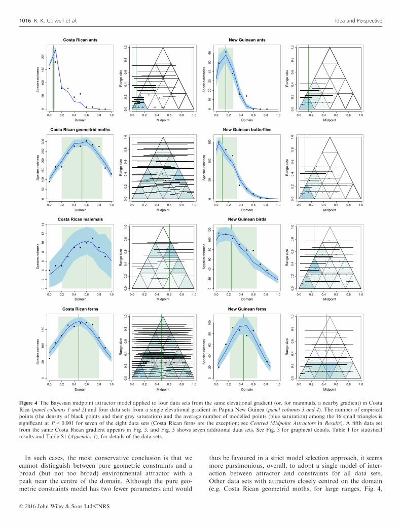
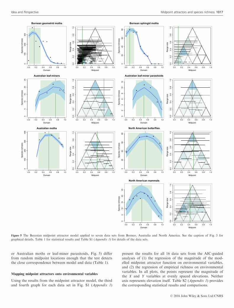
Figure 3 shows the empirical data and the fitted midpointattractor model for the Costa Rican arctiine moth data set.The corresponding graphical results for the other 15 data setsappear in Figs 4 and 5, organised by locality and arranged inthe figures to facilitate comparisons among taxonomically andgeographically related data sets. We emphasise that the graphsfor each data set show the results of 100 simulations using asingle pair of values of the midpoint attractor parameters, Aand B. These ‘best’ parameter values were chosen from theBayesian posterior distribution for the corresponding data set(Fig. S2). For each data set, nearby values of these parametersproduce similar graphs. The spreading dye algorithm (Algo-rithm 2) consistently yielded a fit between modelled andempirical richness that was at least as good, and often better,than the classic approach (Algorithm 1). Consequently, weused the spreading dye algorithm for all data sets in the finalmodels (Table 1).Table 1 displays the quantitative results for midpoint attrac-

tor parameters, and for each, the results for the statisticalcomparisons between modelled and empirical midpoint den-sity patterns within the geometric constraint triangle (rightpanel for each data set in Figs 3–5). For 14 of the 16 datasets, the test affirms a highly significant (mean P < 0.002) cor-respondence between empirical and modelled midpoint densitypatterns. The two exceptions (Costa Rican ferns and NorthAmerican butterflies), instructive in their own right, are dis-cussed below (Centred midpoint attractors).The comparison of modelled and empirical midpoint densi-

ties for large-ranged vs. small-ranged species confirmed theexpectation that both large and small ranges are equally wellfitted by the same midpoint attractor model for most data sets(11 of 16 data sets; Table 1). For a few data sets, a singleattractor may not be an appropriate model. Bornean geome-trid moths and perhaps North American mammals (Fig. 5)show signs of multimodal attractors, although the fit for asimple, unimodal attractor is nonetheless significant.The quantitative results in Table 1 demonstrate the key role

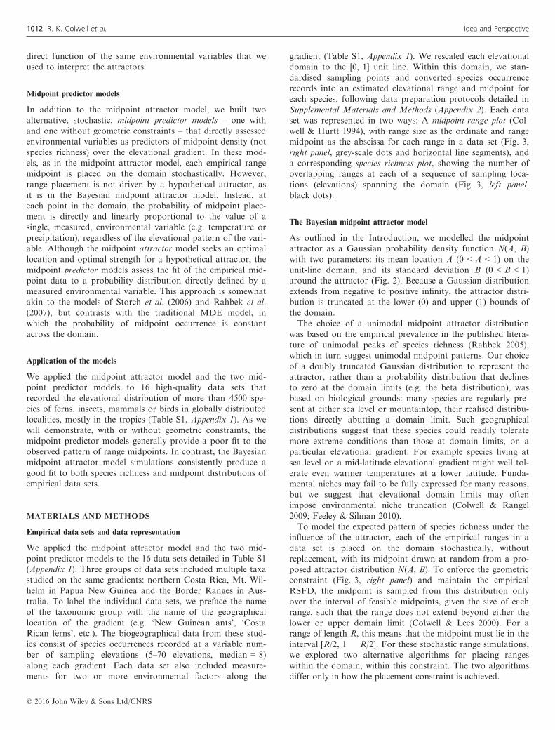
of geometric constraints in the modelled patterns of richness.As expected (Materials and Methods), the closer the modelledattractor is to a domain limit, the greater the discrepancybetween the location of the attractor and the mean locationof range midpoints on the domain (Fig. 6). In terms of thepencil-box analogy (Fig. 1b), the closer the magnet is set toone end of the box, the further the average pencil midpoint isforced away from the box end.Moreover, the shift of mean midpoint locations towards

mid-domain for ranges on gradients with off-centre attractors(Fig. 6) perhaps reconciles our results with the finding of sev-eral previous studies that species richness for small- and large-ranged species is correlated with different environmental fac-tors (e.g. Dunn et al. 2006). Instead, the same environmentalattractors may act differently on small- and large-ranged spe-cies to generate differing distributions. With off-centre attrac-tors, the discordance between attractor and range midpointincreases with range size (e.g. Bornean geometrid moths,Fig. 5). Thus, for larger ranges, patterns of population density

or other indicators of performance or fitness may be asym-metrical around the range midpoint, with the performance orfitness peak lying closer to the attractor than to the rangemidpoint.The fitted standard deviation of the midpoint attractor (pa-

rameter B in the simulations), an inverse measure of thestrength of the attractor, varied from 0.023 (strong attractor)for Costa Rican ants to 0.476 (weak attractor) for NorthAmerican butterflies (Table 1). The location of the midpointattractor (parameter A) on the unit-line domain ranged from0.065 for Costa Rican ants, with nearly monotonically declin-ing richness with elevation, to several data sets with A near0.5 (Costa Rican ferns and geometrid moths, North Americanbutterflies and Australian moths and leaf-miner parasitoids)to 0.742 (Australian leaf miners, on a short, 1100 m gradient).When translated to absolute elevation, A and B vary evenmore strikingly, because the data sets vary from 1100 m to4095 m in elevational scope (Table S1, Appendix 1).How well did the model perform in simulating empirical

richness? The first two graphs for each data set in Fig. S1(Appendix 1) show: (1) the regression of empirical richness onthe magnitude of the modelled midpoint function, and (2) theregression of empirical richness on modelled richness.Table S2 (Appendix 1) provides the corresponding statisticalresults. From these results, we can assess the expectation(Materials and Methods), based on the modelled interactionbetween the attractor and geometric constraints and the fittingmethod itself, that empirical species richness should correlatemore strongly with modelled species richness than with theattractor itself. This expectation was borne out in 12 of the 16data sets. In all but one of the exceptions, the fit of empiricalrichness to modelled richness did not differ, by AIC, from thefit of empirical richness to the attractor. In one data set withrelatively low species richness (Australian leaf-miner para-sitoids), empirical richness was significantly more strongly cor-related with the attractor than with modelled richness.

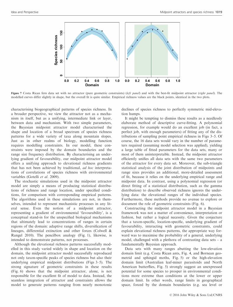
Centred midpoint attractors

When the best-fit attractor lies near the centre of the domain,as it does for Costa Rican ferns and geometrid moths (Fig. 4),North American butterflies (Fig. 5) and Australian moths andleaf-miner parasitoids (Fig. 5) (all with 0.45 < A < 0.55), themodelled pattern of richness may be quite symmetrical – butso is the expected pattern from a simpler MDE model of geo-metric constraints with no environmental drivers. For CostaRican ferns, for example the prediction of the MDE modeldiffers little from the corresponding plot with an optimisedmidpoint attractor (Fig. 7). The sub-triangle statistical test forthe Costa Rican ferns and North American butterfly data setsyields no evidence of an attractor (P > 0.994) (Table 1), nordo the tests for large and small ranges for these two data sets(P > 0.983). Although the modelled and empirical midpointdensities correspond closely in these two data sets, neither dif-fers from a random distribution of midpoints (given theempirical RSFD), necessarily the baseline for judging the pres-ence of an attractor (SI Materials and Methods). Costa Ricangeometrid moths show this same result for small-ranged spe-cies.



In such cases, the most conservative conclusion is that wecannot distinguish between pure geometric constraints and abroad (but not too broad) environmental attractor with apeak near the centre of the domain. Although the pure geo-metric constraints model has two fewer parameters and would

thus be favoured in a strict model selection approach, it seemsmore parsimonious, overall, to adopt a single model of inter-action between attractor and constraints for all data sets.Other data sets with attractors closely centred on the domain(e.g. Costa Rican geometrid moths, for large ranges, Fig. 4,

Figure 4 The Bayesian midpoint attractor model applied to four data sets from the same elevational gradient (or, for mammals, a nearby gradient) in Costa

Rica (panel columns 1 and 2) and four data sets from a single elevational gradient in Papua New Guinea (panel columns 3 and 4). The number of empirical

points (the density of black points and their grey saturation) and the average number of modelled points (blue saturation) among the 16 small triangles is

significant at P < 0.001 for seven of the eight data sets (Costa Rican ferns are the exception; see Centred Midpoint Attractors in Results). A fifth data set

from the same Costa Rican gradient appears in Fig. 3, and Fig. 5 shows seven additional data sets. See Fig. 3 for graphical details, Table 1 for statistical

results and Table S1 (Appendix 1), for details of the data sets.



or Australian moths or leaf-miner parasitoids, Fig. 5) differfrom random midpoint locations enough that the test detectsthe close correspondence between model and data (Table 1).

Mapping midpoint attractors onto environmental variables

Using the results from the midpoint attractor model, the thirdand fourth graph for each data set in Fig. S1 (Appendix 1)

present the results for all 16 data sets from the AIC-guidedanalyses of (1) the regression of the magnitude of the mod-elled midpoint attractor function on environmental variables,and (2) the regression of empirical richness on environmentalvariables. In all plots, the points represent the magnitude ofthe X and Y variables at evenly spaced elevations. Neitheraxis represents elevation itself. Table S2 (Appendix 1) providesthe corresponding statistical results and comparisons.

Figure 5 The Bayesian midpoint attractor model applied to seven data sets from Borneo, Australia and North America. See the caption of Fig. 3 for

graphical details, Table 1 for statistical results and Table S1 (Appendix 1) for details of the data sets.



The environmental variables that best explained the mod-elled midpoint attractor often differed from the environmentalvariables that best predicted observed species richness. Only

three of the 16 data sets yielded an identical statistical model(or model group, when DAIC was < 3 between alternatives), interms of the predictor variables included, for attractor and forspecies richness. However, the model with the lowest absoluteAIC matched in 10 of the 16 data sets, if DAIC-grouped mod-els were ignored (Table S2, illustrated in Fig. S1, Appendix 1).


For each data set, the same environmental variables assessed ininterpreting midpoint attractors (Table S2 and Fig. S1, Appen-dix 1) were tested for the two midpoint predictor models, onewith and the other without geometric constraints. In these mod-els, an environmental variable determined the stochastic place-ment of range midpoints at locations across the domain. Acrossall data sets, 98 of 112 statistical tests (two models, 56 dataset-variable combinations) strongly rejected the null hypothesisthat modelled midpoints resemble the empirical ones, withP < 0.001 in nearly every case (Table S3, Appendix 1). Only fourof the 16 data sets showed an acceptable fit (P > 0.05) to eitherof the midpoint predictor models. But these data sets were, notcoincidentally, the four smallest, in terms of number of species(Australian leaf miners and their parasitoids, Costa Rican andNorth American mammals; Table S1, Appendix 1), and thushad the weakest statistical power to reject the null hypothesis.

DISCUSSION

By modelling and quantifying repeated underlying structures,which we call attractors, we offer a fresh approach to

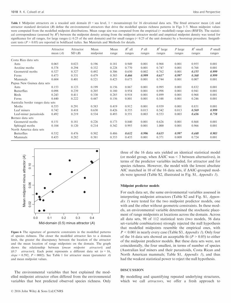
Table 1 Midpoint attractors on a rescaled unit domain (0 = sea level, 1 = mountaintop) for 16 elevational data sets. The fitted attractor mean (A) and

attractor standard deviation (B) define the environmental attractors that drive the modelled species richness patterns in Figs 3–5. Mean midpoint values

were computed from the modelled midpoint distributions. Mean range size was computed from the empirical (= modelled) range sizes (RSFD). The statisti-

cal correspondence (assessed by R2) between the midpoint density arising from the midpoint attractor model and empirical midpoint density was tested for

significance for all ranges, for large ranges (≥ 0.25 of the unit domain) and for small ranges (< 0.25 of the unit domain) by a bootstrap procedure. Insignifi-

cant tests (P > 0.05) are reported in boldfaced italics. See Materials and Methods for details.

Attractor

mean (A)

Attractor

SD (B)

Mean

midpoint

Mean

range

R2 all

ranges

P all

ranges

R2 large

ranges

P large

ranges

R2 small

ranges

P small

ranges

Costa Rica data sets

Ants 0.065 0.023 0.196 0.181 0.949 0.001 0.968 0.001 0.955 0.001

Arctiine moths 0.378 0.294 0.332 0.228 0.770 0.001 0.747 0.001 0.768 0.001

Geometrid moths 0.527 0.327 0.492 0.306 0.650 0.002 0.762 0.001 0.155 0.999

Ferns 0.473 0.331 0.479 0.303 0.466 0.999 0.617 0.997 0.368 0.999

Mammals 0.604 0.401 0.521 0.425 0.675 0.001 0.744 0.001 0.007 0.001

Papua New Guinea data sets

Ants 0.153 0.123 0.199 0.156 0.867 0.001 0.995 0.001 0.832 0.001

Butterflies 0.098 0.239 0.205 0.180 0.954 0.001 0.998 0.001 0.941 0.001

Birds 0.243 0.411 0.330 0.285 0.918 0.001 0.899 0.001 0.968 0.001

Ferns 0.440 0.222 0.447 0.156 0.801 0.001 0.548 0.001 0.246 0.001

Australia border ranges data sets

Moths 0.555 0.291 0.583 0.419 0.912 0.001 0.939 0.001 0.831 0.001

Leaf miners 0.742 0.418 0.630 0.426 0.555 0.015 0.542 0.013 0.569 0.999

Leaf-miner parasitoids 0.492 0.219 0.534 0.493 0.551 0.003 0.553 0.003 0.436 0.758

Borneo data sets

Geometrid moths 0.151 0.181 0.226 0.173 0.840 0.001 0.626 0.001 0.868 0.001

Sphingid moths 0.104 0.120 0.214 0.342 0.993 0.001 1.000 0.001 0.966 0.001

North America data sets

Butterflies 0.532 0.476 0.502 0.486 0.632 0.996 0.635 0.997 0.448 0.983

Mammals 0.435 0.282 0.381 0.353 0.435 0.001 0.371 0.009 0.724 0.001

0.0 0.1 0.2 0.3 0.4

0.02

0.06

0.10

Mid-domain (0.5) minus attractor (A)

Mea

n m

idpo

int m

inus

attr

acto

r (A

)

Figure 6 The signature of geometric constraints in the modelled patterns

of species richness. The closer the modelled attractor lies to a domain

limit, the greater the discrepancy between the location of the attractor

and the mean location of range midpoints on the domain. The graph

shows the relationship between |(mean midpoint � attractor)| and

|(0.5 � attractor)|. Each point represents a different data set (n = 16,

slope = 0.592, P < 0002). See Table 1 for attractor mean (parameter A)

and mean midpoint values.



characterising biogeographical patterns of species richness. Ina broader perspective, we view the attractor not as a mecha-nism in itself, but as a unifying, intermediate link or layer,between data and mechanism. With two simple parameters,the Bayesian midpoint attractor model characterised theshape and location of a broad spectrum of species richnesspatterns for a wide variety of taxa along mountain slopes.Just as in other realms of biology, modelling functionrequires modelling constraints. In our model, these con-straints were imposed by the domain boundaries and therange size frequency distribution. By characterising an under-lying gradient of favourability, our midpoint attractor modeloffers a unifying approach to elevational richness gradientsthat has not been achieved by traditional, ad hoc interpreta-tions of correlations of species richness with environmentalvariables (Gotelli et al. 2009).The stochastic simulations used in the midpoint attractor

model are simply a means of producing statistical distribu-tions of richness and range location, under specified condi-tions, for comparison with corresponding empirical patterns.The algorithms used in these simulations are not, in them-selves, intended to represent mechanistic processes in any lit-eral sense. Even the notion of a midpoint attractor,representing a gradient of environmental ‘favourability’, is aconceptual stand-in for the unspecified biological mechanismsthat ultimately lead to concentrations of ranges in certainregions of the domain: adaptive range shifts, diversification oflineages, differential extinction and other forces (Colwell &Rangel 2010). The pencilbox analogy (Fig. 1), likewise, isintended to demonstrate patterns, not processes.Although the elevational richness patterns successfully mod-

elled in this study varied widely in shape and location on thedomain, the midpoint attractor model successfully reproducednot only taxon-specific peaks of species richness but also theirunderlying empirical midpoint distributions (Figs 3–5). Thestrong signature of geometric constraints in these results(Fig. 6) shows that the midpoint attractor, alone, is notresponsible for the excellent fit of model to data. Instead, theseamless integration of attractor and constraints allows themodel to generate patterns ranging from nearly monotonic

declines of species richness to perfectly symmetric mid-eleva-tion humps.It might be tempting to dismiss these results as a needlessly

elaborate method of descriptive curve-fitting. A polynomialregression, for example would do an excellent job (in fact, aperfect job, with enough parameters) of fitting any of the dis-tributions of sampling point empirical richness in Figs 3–5. Ofcourse, the 16 data sets would vary in the number of parame-ters required (assuming model selection was applied), yieldinga large table of fitted parameters for the data sets, many ormost of them uninterpretable. Instead, the midpoint attractorefficiently unifies all data sets with the same two parametersof the attractor for every data set. Moreover, the sub-trianglestatistical analysis of the joint distribution of midpoints andrange sizes provides an additional, more-detailed assessmentof fit, because it relies on the underlying empirical range andmidpoint data. In contrast, using a polynomial regression (ordirect fitting of a statistical distribution, such as the gammadistribution) to describe observed richness ignores the under-lying data: the elevational ranges of the individual species.Furthermore, these methods provide no avenue to explore ordocument the role of geometric constraints (Fig. 6).Constructing the midpoint attractor model in a Bayesian

framework was not a matter of convenience, interpretation orfashion, but rather a logical necessity. Given the conjecturethat a taxon-specific, location-specific, underlying gradient offavourability, interacting with geometric constraints, couldexplain elevational richness patterns, the appropriate way for-ward was to maximise the probability of a general, underlyingmodel, challenged with a plethora of contrasting data sets – afundamentally Bayesian approach.Data sets with many ranges abutting the low-elevation

domain limit (e.g. Costa Rican ants, Fig. 4, and Bornean geo-metrid and sphingid moths, Fig. 5) or the high-elevationdomain limit (Australian leaf-miner parasitoids and NorthAmerican butterflies, Fig. 5) strongly suggest an unexpressedpotential for some species to prosper in environmental condi-tions more extreme than conditions at the lower or upperdomain limit. In other words, range limits in geographicalspace, forced by the domain boundaries (e.g. sea level or

Figure 7 Costa Rican fern data set with no attractor (pure geometric constraints) (left panel) and with the best-fit midpoint attractor (right panel). The

modelled curves differ slightly in shape, but the overall fit is quite similar. Empirical richness values are the black points, identical in the two plots.



mountaintop), may not coincide with niche limits in nichespace for such species (Colwell & Rangel 2010). The excellentperformance of the doubly truncated Gaussian attractor andour finding that Algorithm 2 (spreading dye) provided a betterfit than Algorithm 1 (classic), considered together, offer sup-port for the inference that ranges that abut domain bound-aries represent niches truncated by the limits of elevationalgradients. In contrast, a species range that reaches neither ofthe domain limits on the gradient may – or may not – fullyexpress the species’ fundamental niche.Shuffling the observed ranges (the RSFD) within a bounded

domain, with or without a midpoint attractor, assumes thatthe RSFD is representative of the size distribution of eleva-tional ranges for a particular taxon on a particular elevationalgradient at the particular time that the data were taken (Col-well et al. 2004). Given that ranges are drawn withoutreplacement from the RSFD and placed randomly on thedomain (within geometric constraints), whereas observedranges tend to be truncated at domain boundaries, the ques-tion then arises: does the midpoint attractor model produce adeficit of small ranges near the domain boundary and anexcess of small ranges in mid-domain? If there were such aneffect, we would expect it to be stronger for attractors locatednearer a domain limit. We tested for this bias by comparingempirical to modelled midpoint density in sub-triangles 10(near sea level), and 7 (mid-domain) (Fig. S3, Appendix 1), asa function of attractor location (A), for the 16 data sets. Wefound no evidence of any pattern of deficiency or excess inmodelled midpoint density. If there is any bias, it is slightenough to be completely masked by the heterogeneous sizeand placement of ranges, both empirical and modelled. Theseresults are consistent with the models of (Colwell & Hurtt1994), who simulated range truncation for a classical MDEmodel, and found very little decrease in mean range size asthe domain boundary was approached.With or without geometric constraints, the midpoint predic-

tor models, which assessed empirical environmental factors ascandidate midpoint predictors, fitted observed elevationalmidpoint distributions very poorly (Table S3, Appendix 1),despite incorporating the empirical RSFD (in one variant)and having two free parameters, just like the midpoint attrac-tor model. For the data sets in this study, the seemingly intu-itive hypothesis that environmental conditions should predictthe location of species range midpoints failed to account formost observed midpoint patterns. In contrast, the midpointattractor model, which, by design, ignores environmental vari-ables, yielded midpoint distributions very close to the empiri-cal midpoint distributions. How can we reconcile this failureof the midpoint predictor model with the success of themidpoint attractor model? At least three, non-exclusive expla-nations are possible: (1) We may have used the ‘wrong’ envi-ronmental variables in the midpoint predictor models.Although the midpoint attractors, together with geometricconstraints, produced a good fit to empirical species richness,the fit of the attractors themselves to environmental variableswas often rather poor (Table S3; third panel in each graph inFig. S1). The original investigators for our data sets measuredimportant aspects of temperature, precipitation and othervariables (such as plant cover) that are believed to affect

species richness on elevational gradients. Primary productivityis thought to be a key correlate of species richness for manygroups (Storch et al. 2006). However, primary productivity isdifficult to measure directly, is difficult to estimate accuratelyon small spatial scales from remotely sensed data, and is miss-ing from all our data sets. (2) We might have analysed theright variables, but we had the wrong functional form. In pre-liminary analyses, however, alternative functional forms (e.g.logarithmic, exponential) did not improve the fit. For many ofour data sets, such as Borneo geometrid moths and New Gui-nea butterflies, the high concentration of species range mid-points in the lower elevations of the domain cannot beaccounted for by any univariate or multivariate transforma-tion of the available environmental variables. (3) Lineagediversification with strong niche conservatism may have pro-duced spatial concentrations of range midpoints in narrowlydefined environments – a sort of theme-and-variations. Con-centrations of elevational range midpoints may arise from‘colonisation’ of new environments (e.g. transitions from low-land to montane specialists) followed by net diversification,with little divergence in environmental tolerances (e.g. Gra-ham et al. 2014; Wu et al. 2014). A search for multimodalattractors and alignment with phylogenetic structure would bea fruitful area of future research.Like niche, or community, or ecosystem, the idea of an envi-

ronmental attractor reifies an abstract construct. Such con-structs endure only if they prove adaptable and useful. In thisstudy, we began with the idea of an attractor, treating it in aBayesian framework as a model to be challenged by eleva-tional data. But the idea of a range attractor model need notbe limited to one-dimensional gradients, nor to terrestrialenvironments. The location and shape of midpoint attractorswithin a particular domain arise from the interactions betweentaxon, climate and history. Comparative study of the relativeinfluence of these factors can be made rigorous and quantita-tive by fitting attractors to multiple data sets, as we have donein this study. The environmental and historical factors defin-ing midpoint attractors in nature are likely to be complex,presenting a challenge for future research. But our approach,in which a modelled midpoint attractor drives the location ofspecies ranges placed stochastically within a bounded domain,may prove more fruitful than further attempts to correlatepatterns of species richness along bounded gradients withenvironmental factors.

ACKNOWLEDGEMENTS

We are grateful to the Editors and to four dedicated, anony-mous reviewers for their incisive and challenging questionsand suggestions, which greatly improved this manuscript. Wethank Paul Lewis for consultation on Bayesian methods. Thisstudy had its origins at a workshop in Ceske Budejovice,Czech Republic, in August, 2013, organised by V. Novotnyand funded by the Czech Ministry of Education and theEuropean Social Fund (CZ.1.07/2.3.00/20.0064). Author sup-port: CAPES Ciencia sem Fronteiras (Brazil) (RKC); U. S.NSF DEB 1257625, DEB 1144055 and DEB 1136644 (NJG);NSF DEB 1354739 (Project ADMAC) (JTL); NSF DEB841885 (JM and VN); Griffith University and Australian



Postgraduate Research Awards (LAA and SCM); AustralianResearch Council DP140101541 (RLK and TMF) and Yaya-san Sime Darby (TMF); German DFG Br 2280/1-1, Fi547/5-1and FOR 402/1-1 (GB and KF); DFG and German AcademicExchange Service DAAD (JK); DFG, Swiss National Fund,& Claraz Schenkung (MK and SN); Czech Science Founda-tion 14-36098G, 14-32302S & 14-32024P (TMF, PK and KS),13-10486S (JM and VN); National Natural Science Founda-tion of China 31370620 (XW); UK Darwin Initiative 19-008(JM and VN); and IBISCA (TMF, KS and LS).

AUTHORSHIP

RKC and NJG conceived and implemented the models, car-ried out the analyses, and drafted the manuscript. RKC pre-pared the figures. LAA, JB, GB, TMF, MLF, KF, MK,RLK, PK, JK, JTL, SCM, CMM, JM, SN, KS, LS and AMScollected or provided data. All authors contributed substan-tially to the development of ideas, the interpretation of resultsand revision of the manuscript.

REFERENCES

Ahrens, C.D. (2013). Meteorology today, (11th edn.). Brooks/Cole

Publishing, Belmont CA, USA.

Albert, C.H., Thuiller, W., Yoccoz, N.G., Soudant, A., Boucher, F.,

Saccone, P. et al. (2010). Intraspecific functional variability: extent,

structure and sources of variation. J. Ecol., 98, 604–613.Allen, A.P., Gillooly, J.F. & Brown, J.H. (2007). Recasting the species-

energy hypothesis: the different roles of kinetic and potential energy in

regulating biodiversity. In: Scaling Biodiversity (eds. Storch, D,

Marquet, PA & Brown, JH). Cambridge University Press Cambridge,

UK, pp. 283–299.Chan, W.-P., Chen, I.-C., Colwell, R.K., Liu, W.-C., Huang, C.-Y. &

Shen, S.-F. (2016). Seasonal and daily climate variation have opposite

effects on species elevational range size. Science, 351, 1437–1439.Colwell, R.K. & Hurtt, G.C. (1994). Nonbiological gradients in species

richness and a spurious Rapoport effect. Am. Nat., 144, 570–595.Colwell, R.K. & Lees, D.C. (2000). The mid-domain effect: geometric

constraints on the geography of species richness. Trends Ecol. Evol., 15,

70–76.Colwell, R.K. & Rangel, T.F. (2009). Hutchinson’s duality: the once and

future niche. PNAS, 106, 19651–19658.Colwell, R.K. & Rangel, T.F. (2010). A stochastic, evolutionary model

for range shifts and richness on tropical elevational gradients under

Quaternary glacial cycles. Philos. Trans. R. Soc. Lond. B Biol. Sci., 365,

3695–3707.Colwell, R.K., Rahbek, C. & Gotelli, N. (2004). The mid-domain effect

and species richness patterns: what have we learned so far? Am. Nat.,

163, E1–E23.Colwell, R.K., Rahbek, C. & Gotelli, N. (2005). The mid-domain effect:

there’s a baby in the bathwater. Am. Nat., 166, E149–E154.Connolly, S.R. (2005). Process-based models of species distributions and

the middomain effect. Am. Nat., 166, 1–11.Currie, D.J. & Kerr, J.T. (2008). Tests of the mid-domain hypothesis: a

review of the evidence. Ecol. Monogr., 78, 3–18.Currie, D., Mittelbach, G., Cornell, H., Field, R., Guegan, J., Hawkins,

B. et al. (2004). Predictions and tests of climate-based hypotheses of

broad-scale variation in taxonomic richness. Ecol. Lett., 7, 1121–1134.Dunn, R.R., Colwell, R.K. & Nilsson, C. (2006). The river domain: why

are there more species halfway up the river? Ecography, 29, 251–259.Dunn, R.R., McCain, C.M. & Sanders, N. (2007). When does diversity fit

null model predictions? Scale and range size mediate the mid-domain

effect. Glob. Ecol. Biogeogr., 3, 305–312.

Fan, Y. & van den Dool, H. (2008). A global monthly land surface

air temperature analysis for 1948-present. J. Geophys. Res., 113,

D01103.

Feeley, K.J. & Silman, M.R. (2010). Biotic attrition from tropical forests

correcting for truncated temperature niches. Global Change Biol., 16,

1830–1836.Gelman, A., Carlin, J.B., Stern, H.S., Dunson, D.B., Vehtari, A. &

Rubin, D.B. (2013). Bayesian Data Analysis. CRC Press, Boca Raton,

FL, USA.

Gotelli, N., Anderson, M.J., Arita, H.T., Chao, A., Colwell, R.K.,

Connolly, S.R. et al. (2009). Patterns and causes of species richness: a

general simulation model for macroecology. Ecol. Lett., 12, 873–886.Graham, C.H., Carnaval, A.C., Cadena, C.D., Zamudio, K.R., Roberts,

T.E., Parra, J.L. et al. (2014). The origin and maintenance of montane

diversity: integrating evolutionary and ecological processes. Ecography,

37, 711–719.Grytnes, J. (2003). Ecological interpretations of the mid-domain effect.

Ecol. Lett., 6, 883–888.Grytnes, J.A., Beaman, J.H., Romdal, T.S. & Rahbek, C. (2008). The mid-

domain effect matters: simulation analyses of range-size distribution data

from Mount Kinabalu. Borneo. J. Biogeogr., 35, 2138–2147.Hartig, F., Calabrese, J.M., Reineking, B., Wiegand, T. & Huth, A.

(2011). Statistical inference for stochastic simulation models – theory

and application. Ecol. Lett., 14, 816–827.Hawkins, B.A., Field, R., Cornell, H.V., Currie, D.J., Gu�egan, J.-F.,

Kaufmann, D.M. et al. (2003). Energy, water, and broad-scale

geographic patterns of species richness. Ecology, 84, 3105–3117.Jetz, W. & Rahbek, C. (2001). Geometric constraints explain much of the

species richness pattern in African birds. PNAS, 98, 5661–5666.Laurie, H. & Silander Jr., J.A. (2002). Geometric constraints and spatial

pattern of species richness: critique of range-based null models. Divers.

Distrib., 8, 351–364.Letten, A.D., Kathleen Lyons, S. & Moles, A.T. (2013). The mid-domain

effect: it’s not just about space. J. Biogeogr., 40, 2017–2019.Lomolino, M.V. (2001). Elevational gradients of species density: historical

and prospective views. Global Ecol. Biogeogr., 10, 3–13.Longino, J.T. & Colwell, R.K. (2011). Density compensation, species

composition, and richness of ants on a neotropical elevational gradient.

Ecosphere, 2(3), art. 29. doi:10.1890/ES10-00200.1.

Longino, J.T., Branstetter, M.G. & Colwell, R.K. (2014). How ants drop

out: ant abundance on tropical mountains. PLoS ONE, 9, e104030.

Marjoram, P., Molitor, J., Plagnol, V. & Tavar�e, S. (2003). Markov chain

Monte Carlo without likelihoods. Proc. Natl. Acad. Sci. U. S. A., 100,

15324.

McCain, C.M. (2007). Could temperature and water availability drive

elevational species richness patterns? A global case study for bats. Glob.

Ecol. Biogeogr., 16, 1–13.McCain, C.M. & Grytnes, J.A. (2010). Elevational gradients in species

richness. In: Encyclopedia of Life Sciences (ELS) (ed. Janson, R.).

John Wiley & Sons, Ltd, Chichester, UK.

Newbery, D. & Lingenfelder, M. (2009). Plurality of tree species

responses to drought perturbation in Bornean tropical rain forest.

Forest Ecology 201, 147–167.Presley, S.J., Willig, M.R., Bloch, C.P., Castro-Arellano, I., Higgins, C.L.

& Klingbeil, B.T. (2011). A complex metacommunity structure for

gastropods along an elevational gradient. Biotropica, 43, 480–488.Prevedello, J.A., Figueiredo, M.S., Grelle, C.E. & Vieira, M.V. (2013).

Rethinking edge effects: the unaccounted role of geometric constraints.

Ecography, 36, 287–299.Rahbek, C. (1995). The elevational gradient of species richness: a uniform

pattern? Ecography, 19, 200–205.Rahbek, C. (2005). The role of spatial scale in the perception of large-

scale species-richness patterns. Ecol. Lett., 8, 224–239.Rahbek, C., Gotelli, N., Colwell, R.K., Entsminger, G.L., Rangel,

T.F.L.V.B. & Graves, G.R. (2007). Predicting continental-scale patterns

of bird species richness with spatially explicit models. Proc. Biol. Sci.,

274, 165–174.



http://dx.doi.org/10.1890/ES10-00200.1

Rangel, T.F.L.V.B. & Diniz-Filho, J.A.F. (2005). An evolutionary

tolerance model explaining spatial patterns in species richness under

environmental gradients and geometric constraints. Ecography, 28, 253–263.

Rangel, T.F., Diniz Filho, J.A.F. & Bini, L.M. (2010). SAM: a

comprehensive application for Spatial Analysis in Macroecology.

Ecography, 33, 46–50.Storch, D., Davies, R.G., Zajicek, S., Orme, C.D.L., Olson, V., Thomas,

G.H. et al. (2006). Energy, range dynamics and global species richness

patterns: reconciling mid-domain effects and environmental

determinants of avian diversity. Ecol. Lett., 9, 1308–1320.Sundqvist, M.K., Giesler, R., Graae, B.J., Wallander, H., Fogelberg, E. &

Wardle, D.A. (2011). Interactive effects of vegetation type and

elevation on aboveground and belowground properties in a subarctic

tundra. Oikos, 120, 128–142.Tiwari, M., Bjorndal, K.A., Bolten, A.B. & Bolker, B.M. (2005).

Intraspecific application of the mid-domain effect model: spatial and

temporal nest distributions of green turtles, Chelonia mydas, at

Tortuguero, Costa Rica. Ecol. Lett., 8, 918–924.Wang, X. & Fang, J. (2012). Constraining null models with

environmental gradients: a new method for evaluating the effects of

environmental factors and geometric constraints on geographic

diversity patterns. Ecography, 35, 1147–1159.Wright, S.J., Muller-Landau, H. & Schipper, J. (2009). The future of

tropical species on a warmer planet. Conserv. Biol., 23, 1418–1426.Wu, Y., Colwell, R.K., Han, N., Zhang, R., Wang, W., Quan, Q. et al.

(2014). Understanding historical and current patterns of species

richness of babblers along a 5000-m subtropical elevational gradient.

Global Ecol. Biogeogr., 23, 1167–1176.

SUPPORTING INFORMATION

Additional Supporting Information may be found online inthe supporting information tab for this article.

Editor, Nathan SwensonManuscript received 20 January 2016First decision made 28 February 2016Manuscript accepted 18 May 2016



PERSPECTIVE Midpoint attractors and species richness...

Documents

Transcript of PERSPECTIVE Midpoint attractors and species richness...