Personality Traits and Drug Consumption - arXiv.org e ...
134
Elaine Fehrman, Vincent Egan, Alexander N. Gorban, Jeremy Levesley, Evgeny M. Mirkes, Awaz K. Muhammad Personality Traits and Drug Consumption A Story Told by Data Springer arXiv:2001.06520v1 [stat.AP] 17 Jan 2020
Transcript of Personality Traits and Drug Consumption - arXiv.org e ...

Elaine Fehrman, Vincent Egan,Alexander N. Gorban, Jeremy Levesley,Evgeny M. Mirkes, Awaz K. Muhammad
Personality Traits and Drug Consumption
A Story Told by Data
Springer
arX
iv:2
001.
0652
0v1
[st
at.A
P] 1
7 Ja
n 20
20

v
Abstract In this book a story is told about the psychological traits associated with drug consumption. Thebook includes:
• A review of published works on the psychological profiles of drug users.• Analysis of a new original database with information on 1885 respondents and usage of 18 drugs. (Database
is available online.)• An introductory description of the data mining and machine learning methods used for the analysis of this
dataset.• The demonstration that the personality traits (five factor model, impulsivity, and sensation seeking),
together with simple demographic data, give the possibility of predicting the risk of consumption ofindividual drugs with sensitivity and specificity above 70% for most drugs.
• The analysis of correlations of use of different substances and the description of the groups of drugs withcorrelated use (correlation pleiades).
• Proof of significant differences of personality profiles for users of different drugs. This is explicitly provedfor benzodiazepines, ecstasy, and heroin.
• Tables of personality profiles for users and non-users of 18 substances.
The book is aimed at advanced undergraduates or first-year PhD students, as well as researchers and practi-tioners. No previous knowledge of machine learning, advanced data mining concepts or modern psychologyof personality is assumed. For more detailed introduction into statistical methods we recommend severalundergraduate textbooks. Familiarity with basic statistics and some experience in the use of probabilitieswould be helpful as well as some basic technical understanding of psychology.

Preface
Each set of data can tell us a story. Our mission is to extract this story from the data and translate it into morereadily accessible human language. There are a number of tools for such a translation. To prepare this storywe have to collect data, to ask interesting questions and to apply all the possible data mining technical toolsto find the answers. Then we should verify the answers, exclude spurious (overoptimistic) correlations andpatterns, and tell the story to users.
The topic of mining interesting knowledge remains very intriguing. Many researchers have approached thisproblem from a plethora of different angles. One of the main ideas in these approaches has been informationgain (the more information gain there is, the more interesting the result is). Nevertheless, we need a goodunderstanding of what makes patterns that are found interesting from the end-user’s point of view. Herevarious perspectives might be involved, from practical importance to aesthetic beauty. The extraction of deepand interesting knowledge from data was formulated as an important problem for the 5th IEEE InternationalConference on Data Mining (ICDM 2005) [1]. Nowadays, the fast growth of the fields of data science andmachine learning provides us with many tools for answering such questions, but the art of asking interestingquestions still requires human expertise.
The practical importance of the problem of evaluating an individual’s risk of consuming and/or abusingdrugs cannot be underestimated [2]. One might well ask how this risk depends on a multitude of possiblefactors [3]? The linking of personality traits to risk of substance use disorder is an enduring problem [4].Researchers return again and again to this problem following the collection of new data, and with newquestions.
How do personality, gender, education, nationality, age, and other attributes affect this risk? Is thisdependence different for different drugs? For example, does the risk of ecstasy consumption and the risk ofheroin consumption differ for different personality profiles? Which personality traits are the most importantfor evaluation of the risk of consumption of a particular drug, and are these traits different for different drugs?These questions are the focus of our research.
The data set we collected contains information on the consumption of 18 central nervous system psychoac-tive drugs, by 2,051 respondents (after cleaning, 1,885 participants remained, male/female = 943/942). Thedatabase is available online [5, 6].
The questions we pose above have been reformulated as classification problems and many well-knowndata mining methods have been employed to address these problems: decision trees, random forests, k-nearestneighbours, linear discriminant analysis, Gaussian mixtures, probability density function estimation usingradial basis functions, logistic regression and naıve Bayes. For data preprocessing, transformation and ranking
vii

viii Preface
we have used methods such as polychoric correlation, nonlinear CatPCA (Categorical Principal ComponentAnalysis), sparse PCA, and original double Kaiser’s feature selection.
The main results of the work are:
• The presentation and descriptive analysis of a database with information on 1,885 respondents and theirusage of 18 drugs.
• Demonstration that the personality traits (Five Factor Model [7], impulsivity, and sensation-seeking)together with simple demographic data give the possibility of predicting the risk of consumption ofindividual drugs with sensitivity and specificity above 70% for most drugs.
• The construction of the best classifiers and most significant predictors for each individual drug in question.• Revelation of significantly distinct personality profiles for users of different drugs; in particular, groups of
heroin and ecstasy users are significantly different in Neuroticism (higher for heroin), Extraversion (higherfor ecstasy), Agreeableness (higher for Ecstasy), and Impulsivity (higher for heroin); groups of heroin andbenzodiazepine users are significantly different in Agreeableness (higher for benzodiazepines), Impulsivity(higher for heroin), and Sensation-Seeking (higher for heroin); groups of ecstasy and benzodiazepine usersare significantly different in Neuroticism (higher for benzodiazepines), Extraversion (higher for ecstasy),Openness to Experience (higher for ecstasy), and Sensation-Seeking (higher for ecstasy).
• The discovery of three correlation pleiades of drugs; these are the clusters of drugs with correlatedconsumption centered around heroin, ecstasy, and benzodiazepines. The correlation pleiades shouldinclude the mini-sequences of drug involvement found in longitudinal studies [8], and aim to serve asmaps for analysis of different patterns of influence.
• The development of risk map technology for the visualization of the probability of drug consumption.
Four of the authors (ANG, JL, EMM, and AKM) are applied mathematicians and two are psychologists(EF and VE). Data were collected by EF and processed by EMM and AKM. The psychological frameworkfor this study was developed by EF and VE, and the analytic methodology was selected and developed byANG and EMM. The final results were critically analysed and described by ANG, JL, EMM, and AKM fromthe data mining perspective, and EF and VE provided the psychological interpretation and conceptualization.
For psychologists, the book gives a new understanding of the relationship between personality traits andthe usage of 18 psychoactive substances, provides a new openly available database for further study, andpresents many useful methods of data analysis. For applied mathematicians and statisticians, the book detailsa case study in a fascinating area of application, exemplifying the use of various data mining methods in suchscenarios.
This book is aimed at advanced undergraduates or first-year PhD students, as well as researchers andpractitioners in data analysis, applied mathematics and psychology. No previous knowledge of machinelearning, advanced data mining concepts or psychology of personality is assumed. Familiarity with basicstatistics and some experience of the use of probability is helpful, as well as some basic understanding ofpsychology. Two books [9, 10] include all the necessary prerequisites (and much more). Linear DiscriminantAnalysis (LDA), Principal Component Analysis (PCA), and Decision Trees (DT) are systematically employedin the book. Therefore, it may be useful to refresh the knowledge of these classical methods using the textbook[10], which is concentrated more on the applications of the methods and less on the mathematical details.
A preliminary report of our work was published as an arXiv e-print in 2015 [11] and presented at theConference of International Federation of Classification Societies 2015 (IFCS 2015) [12].
This book is not the end of the story told by the data. We will continue our work and try to extract moreinteresting knowledge and patterns from the data. Moreover, we are happy for you, the readers, to join us inthis adventure. We believe that every large annotated dataset is a treasure trove and that there is an abundanceof interesting knowledge to discover from them. We have published our database online [5, 6] and invite
References ix
everybody to use it for their own projects, from BSc and MSc level to PhD, or just for curiosity-drivenresearch. We would be very happy to see the fascinating outcomes of these projects.
References
1. Yang, Q., Wu, X.: 10 challenging problems in data mining research. Int. J. Inf. Technol. & Decis. Mak. 5(04), 597–604(2006). doi:10.1142/S0219622006002258
2. United Nations Office on Drugs and Crime: World drug report 2016. United Nations, New Yorkhttp://www.unodc.org/wdr2016/ (2016). Accessed 27 Dec 2017
3. Hawkins, J.D., Catalano, R.F., Miller, J.Y.: Risk and protective factors for alcohol and other drug problems in adolescenceand early adulthood: implications for substance abuse prevention. Psychol. bull. 112(1), 64–105 (1992). doi:10.1037/0033-2909.112.1.64
4. Kotov, R., Gamez, W., Schmidt, F., Watson, D.: Linking big personality traits to anxiety, depressive, and substance usedisorders: A meta-analysis. Psychol. bull. 136(5), 768–821 (2010). doi:10.1037/a0020327
5. Fehrman, E., Egan, V.: Drug consumption, collected online March 2011 to March 2012, English-speaking countries.ICPSR36536-v1. Ann Arbor, MI: Inter-university Consortium for Political and Social Research [distributor] (2016).Deposited by Mirkes, E.M. doi:10.3886/ICPSR36536.v1
6. Fehrman, E., Egan, V., Mirkes, E.M.: Drug consumption (quantified) data set. UCI Machine Learning Repository (2016).https://archive.ics.uci.edu/ml/datasets/Drug+consumption+%28quantified%29 Accessed 27 Dec 2017
7. Costa, P.T., MacCrae, R.R.: Revised NEO-personality inventory (NEO PI-R) and NEO five-factor inventory (NEO FFI):Professional manual. Psychological Assessment Resources, Odessa, FL (1992)
8. Newcomb M.D., Bentler, P.M.: Frequency and sequence of drug use: A longitudinal study from early adolescence to youngadulthood. J. Drug Educ. 16(2), 101–120 (1986). doi:10.2190/1VKR-Y265-182W-EVWT
9. Corr, P.J., Matthews, G. (ed.): The Cambridge handbook of personality psychology. Cambridge University Press, New York(2009). doi:10.1017/cbo9780511596544
10. James, G., Witten, D., Hastie, T., Tibshirani, R.: An introduction to statistical learning. Springer Texts in Statistics vol. 103,Springer, New York (2013). doi:10.1007/978-1-4614-7138-7
11. Fehrman, E., Muhammad, A.K., Mirkes, E.M., Egan, V., Gorban, A.N.: The five factor model of personality and evaluationof drug consumption risk. ArXiv preprint https://arxiv.org/abs/1506.06297 (2015). Accessed 27 Dec 2017
12. Fehrman, E., Muhammad, A.K., Mirkes, E.M., Egan, V., Gorban, A.N.: The five factor model of personality and evaluationof drug consumption risk. In: Palumbo, F., Montanari, A., Vichi, M. (eds.), Data Science, Studies in Classification, DataAnalysis, and Knowledge Organization, pp. 215–226, Springer, Cham (2017). doi:10.1007/978-3-319-55723-6 18
Leicester – Nottingham, Elaine FehrmanDecember 2017 Vincent Egan
Alexander N. GorbanJeremy Levesley
Evgeny M. MirkesAwaz K. Muhammad

Contents
1 Introduction: drug use and personality profiles . . . . . . . . . . . . . . . . . . . . . . . . . . . . . . . . . . . . . . . . 11.1 Definitions of drugs and drug usage . . . . . . . . . . . . . . . . . . . . . . . . . . . . . . . . . . . . . . . . . . . . . . . 11.2 Personality traits . . . . . . . . . . . . . . . . . . . . . . . . . . . . . . . . . . . . . . . . . . . . . . . . . . . . . . . . . . . . . . . 21.3 How many inputs do the predictive models have: 5, 30, 60, or 240? . . . . . . . . . . . . . . . . . . . . . 31.4 The problem of the relationship between personality traits and drug consumption . . . . . . . . . 41.5 New dataset open for use . . . . . . . . . . . . . . . . . . . . . . . . . . . . . . . . . . . . . . . . . . . . . . . . . . . . . . . . 111.6 First results in brief . . . . . . . . . . . . . . . . . . . . . . . . . . . . . . . . . . . . . . . . . . . . . . . . . . . . . . . . . . . . . 14References . . . . . . . . . . . . . . . . . . . . . . . . . . . . . . . . . . . . . . . . . . . . . . . . . . . . . . . . . . . . . . . . . . . . . . . . . 18
2 Methods of Data Analysis . . . . . . . . . . . . . . . . . . . . . . . . . . . . . . . . . . . . . . . . . . . . . . . . . . . . . . . . . . . 232.1 Preprocessing . . . . . . . . . . . . . . . . . . . . . . . . . . . . . . . . . . . . . . . . . . . . . . . . . . . . . . . . . . . . . . . . . . 23
2.1.1 Descriptive statistics: mean, variance, covariance, correlation, information gain . . . . 232.1.2 Input feature normalization . . . . . . . . . . . . . . . . . . . . . . . . . . . . . . . . . . . . . . . . . . . . . . . . 25
2.2 Input feature transformation . . . . . . . . . . . . . . . . . . . . . . . . . . . . . . . . . . . . . . . . . . . . . . . . . . . . . . 262.2.1 Principal Component Analysis – PCA . . . . . . . . . . . . . . . . . . . . . . . . . . . . . . . . . . . . . . . 262.2.2 Quantification of categorical input variables . . . . . . . . . . . . . . . . . . . . . . . . . . . . . . . . . . 272.2.3 Input feature ranking . . . . . . . . . . . . . . . . . . . . . . . . . . . . . . . . . . . . . . . . . . . . . . . . . . . . . 30
2.3 Classification and risk evaluation . . . . . . . . . . . . . . . . . . . . . . . . . . . . . . . . . . . . . . . . . . . . . . . . . 312.3.1 Single attribute predictors . . . . . . . . . . . . . . . . . . . . . . . . . . . . . . . . . . . . . . . . . . . . . . . . . 312.3.2 Criterion for selecting the best method . . . . . . . . . . . . . . . . . . . . . . . . . . . . . . . . . . . . . . 332.3.3 Linear Discriminant Analysis (LDA) . . . . . . . . . . . . . . . . . . . . . . . . . . . . . . . . . . . . . . . . 332.3.4 Logistic Regression (LR) . . . . . . . . . . . . . . . . . . . . . . . . . . . . . . . . . . . . . . . . . . . . . . . . . . 342.3.5 k Nearest Neighbours (kNN) . . . . . . . . . . . . . . . . . . . . . . . . . . . . . . . . . . . . . . . . . . . . . . . 342.3.6 Decision Tree (DT) . . . . . . . . . . . . . . . . . . . . . . . . . . . . . . . . . . . . . . . . . . . . . . . . . . . . . . 352.3.7 Random Forest (RF) . . . . . . . . . . . . . . . . . . . . . . . . . . . . . . . . . . . . . . . . . . . . . . . . . . . . . . 372.3.8 Gaussian Mixture (GM) . . . . . . . . . . . . . . . . . . . . . . . . . . . . . . . . . . . . . . . . . . . . . . . . . . . 372.3.9 Probability Density Function Estimation (PDFE) . . . . . . . . . . . . . . . . . . . . . . . . . . . . . . 382.3.10 Naıve Bayes (NB) . . . . . . . . . . . . . . . . . . . . . . . . . . . . . . . . . . . . . . . . . . . . . . . . . . . . . . . 38
2.4 Visualisation on the non-linear PC canvas: Elastic maps . . . . . . . . . . . . . . . . . . . . . . . . . . . . . . 38References . . . . . . . . . . . . . . . . . . . . . . . . . . . . . . . . . . . . . . . . . . . . . . . . . . . . . . . . . . . . . . . . . . . . . . . . . 40
xi

xii Contents
3 Results of data analysis . . . . . . . . . . . . . . . . . . . . . . . . . . . . . . . . . . . . . . . . . . . . . . . . . . . . . . . . . . . . . 453.1 Descriptive statistics and psychological profile of illicit drug users . . . . . . . . . . . . . . . . . . . . . 453.2 Distribution of number of drugs used . . . . . . . . . . . . . . . . . . . . . . . . . . . . . . . . . . . . . . . . . . . . . . 493.3 Sample mean and population norm . . . . . . . . . . . . . . . . . . . . . . . . . . . . . . . . . . . . . . . . . . . . . . . . 503.4 Deviation of the groups of drug users from the sample mean . . . . . . . . . . . . . . . . . . . . . . . . . . . 533.5 Significant differences between groups of drug users and non-users . . . . . . . . . . . . . . . . . . . . . 563.6 Correlation between usage of different drugs . . . . . . . . . . . . . . . . . . . . . . . . . . . . . . . . . . . . . . . 583.7 Ranking of input features . . . . . . . . . . . . . . . . . . . . . . . . . . . . . . . . . . . . . . . . . . . . . . . . . . . . . . . . 613.8 Selection of the best classifiers for the decade-based classification problem . . . . . . . . . . . . . . 633.9 Correlation pleiades of drugs . . . . . . . . . . . . . . . . . . . . . . . . . . . . . . . . . . . . . . . . . . . . . . . . . . . . . 663.10 Overoptimism problem . . . . . . . . . . . . . . . . . . . . . . . . . . . . . . . . . . . . . . . . . . . . . . . . . . . . . . . . . . 723.11 User/non-user classification by linear discriminant for ecstasy and heroin . . . . . . . . . . . . . . . 733.12 Separation of heroin users from ecstasy users: what is the difference? . . . . . . . . . . . . . . . . . . 773.13 Significant difference between benzodiazepines, ecstasy, and heroin . . . . . . . . . . . . . . . . . . . . 803.14 A tree of linear discriminants: no essential improvements . . . . . . . . . . . . . . . . . . . . . . . . . . . . . 823.15 Visualisation on non-linear PCA canvas . . . . . . . . . . . . . . . . . . . . . . . . . . . . . . . . . . . . . . . . . . . 853.16 Risk maps . . . . . . . . . . . . . . . . . . . . . . . . . . . . . . . . . . . . . . . . . . . . . . . . . . . . . . . . . . . . . . . . . . . . . 85References . . . . . . . . . . . . . . . . . . . . . . . . . . . . . . . . . . . . . . . . . . . . . . . . . . . . . . . . . . . . . . . . . . . . . . . . . 86
Summary . . . . . . . . . . . . . . . . . . . . . . . . . . . . . . . . . . . . . . . . . . . . . . . . . . . . . . . . . . . . . . . . . . . . . . . . . . . . . . 93References . . . . . . . . . . . . . . . . . . . . . . . . . . . . . . . . . . . . . . . . . . . . . . . . . . . . . . . . . . . . . . . . . . . . . . . . . 97
Discussion . . . . . . . . . . . . . . . . . . . . . . . . . . . . . . . . . . . . . . . . . . . . . . . . . . . . . . . . . . . . . . . . . . . . . . . . . . . . 99References . . . . . . . . . . . . . . . . . . . . . . . . . . . . . . . . . . . . . . . . . . . . . . . . . . . . . . . . . . . . . . . . . . . . . . . . . 100
Main tables . . . . . . . . . . . . . . . . . . . . . . . . . . . . . . . . . . . . . . . . . . . . . . . . . . . . . . . . . . . . . . . . . . . . . . . . . . . . 101A.1 Psychological profiles of drug users and non-users . . . . . . . . . . . . . . . . . . . . . . . . . . . . . . . . . . . 101A.2 Correlation between consumption of different drugs . . . . . . . . . . . . . . . . . . . . . . . . . . . . . . . . . . 111A.3 Linear discriminants for user/non-user separation . . . . . . . . . . . . . . . . . . . . . . . . . . . . . . . . . . . . 113
Chapter 1Introduction: drug use and personality profiles
1.1 Definitions of drugs and drug usage
Since Sir Karl Popper, it has become a commonplace opinion in the philosophy of science that the ‘value’ ofdefinitions, other than for mathematics, is generally unhelpful. Nevertheless, for many more practical spheresof activity, from jurisprudence to health planning, definitions are necessary to impose theoretical boundarieson a subject, in spite of their incompleteness and their tendency to change with time. This applies strongly todefinitions of drugs and drug use.
Following the standard definitions [1],
• A drug is a ‘chemical that influences biological function (other than by providing nutrition or hydration)’.• A psychoactive drug is a ‘drug whose influence is in a part on mental functions’.• An abusable psychoactive drug is a ‘drug whose mental effects are sufficiently pleasant or interesting or
helpful that some people choose to take it for a reason other than to relieve a specific malady’.
In our study we use the term ‘drug’ for abusable psychoactive drug regardless of whether it is illicit or not.While legal substances such as sugar, alcohol and tobacco are probably responsible for far more prematuredeath than illegal recreational drugs [2], the social and personal consequences of recreational drug use can behighly problematic [3].
Use of drugs introduces risk into a life across a broad spectrum; it constitutes an important factor forincreasing risk of poor health, along with earlier mortality and morbidity, and has significant consequencesfor society [4, 5]. Drug consumption and addiction constitutes a serious problem globally. Though drug use isargued by civil libertarians to be a matter of individual choice, the effects on an individual of drug use such asgreater mortality or lowered individual functioning, suggest that drug use has social and interpersonal effectson individuals who have not chosen to use drugs themselves.
Several terms are used to characterise drug use disorder: addiction, dependence, and abuse. For a longtime, ‘substance abuse’ and ‘substance dependence’ were considered as separate disorders. In 2013, TheDiagnostic and Statistical Manual of Mental Disorders (DSM-5) joined these two diagnoses into ‘SubstanceUse Disorder’ [6]. This is a more inclusive term used to identify persons with substance-related problems.More recently, abuse and dependence have been defined on a scale that measures the time and degree ofsubstance use. Criteria are provided for substance use disorder, supplemented by criteria for intoxication,withdrawal, substance/medication-induced disorders, and unspecified substance-induced disorders, whererelevant. Abuse can be considered as the early stage of substance use disorder.
1

2 1 Introduction: drug use and personality profiles
In our study we differentiate the substance users on the basis of recency of use but do not identify existenceand depth of the substance dependence.
For prevention and effective care of substance use disorder, we need to identify the risk factors and developmethods for their evaluation and control [7].
1.2 Personality traits
Sir Francis Galton (1884) proposed that a lexical approach in which one used dictionary definitions ofdispositions could be a means of constructing a description of individual differences (see [8]). He selected thepersonality-descriptive terms and stated the problem of their interrelations. In 1934, Thurstone [9] selected60 adjectives that are in common use for describing people and asked each of 1300 respondents to think ofa person they knew well and to select the adjectives that can best describe this person. After studying thecorrelation matrix he found that five factors are sufficient to describe this choice.
There have been many versions of the five factor model proposed since Thurston [10], for example:
• Surgency, agreeableness, dependability, emotional stability, and culture;• Surgency, agreeableness, conscientiousness, emotional stability, and culture;• Assertiveness, likeability, emotionality, intelligence, and responsibility;• Social adaptability, conformity, will to achieve, emotional control, and inquiring intellect;• Assertiveness, likeability, task interest, emotionality, and intelligence;• Extraversion, friendly compliance, will to achieve, neuroticism, and intellect;• Power, love, work, affect, and intellect;• Interpersonal involvement, level of socialization, self-control, emotional stability, independence.
There are also systems with different numbers of factors (three, seven, etc.). The most important three-factorsystem is Eysenck’s model comprising extraversion, psychoticism, and neuroticism.
Nowadays, after many years of research and development, psychologists have largely agreed that thepersonality traits of the modern Five Factor Model (FFM) constitutes the most comprehensive and adapt-able system for understanding human individual differences [11]. The FFM comprises Neuroticism (N),Extraversion (E), Openness to Experience (O), Agreeableness (A), and Conscientiousness (C).
The five traits can be summarized thus:
N Neuroticism is a long-term tendency to experience negative emotions such as nervousness, tension,anxiety and depression (associated adjectives [12]: anxious, self-pitying, tense, touchy, unstable, andworrying);
E Extraversion manifested in characters who are outgoing, warm, active, assertive, talkative, and cheer-ful; these persons are often in search of stimulation (associated adjectives: active, assertive, energetic,enthusiastic, outgoing, and talkative);
O Openness to experience is associated with a general appreciation for art, unusual ideas, and imaginative,creative, unconventional, and wide interests (associated adjectives: artistic, curious, imaginative, insightful,original, and wide interest);
A Agreeableness is a dimension of interpersonal relations, characterized by altruism, trust, modesty,kindness, compassion and cooperativeness (associated adjectives: appreciative, forgiving, generous, kind,sympathetic, and trusting);
C Conscientiousness is a tendency to be organized and dependable, strong-willed, persistent, reliable, andefficient (associated adjectives: efficient, organised, reliable, responsible, and thorough).
1.3 How many inputs do the predictive models have: 5, 30, 60, or 240? 3
Individuals low on the A and C trait dimensions have less incidence of the reported attributes, so, for example,lower Agreeableness is associated with greater antisocial behaviour [89].
1.3 How many inputs do the predictive models have: 5, 30, 60, or 240?
The NEO PI-R questionnaire was specifically designed to measure the FFM of personality [11]. It providesscores corresponding to N, E, O, A, and C (‘domain scores’). The NEO PI-R consists of 240 self-report itemsanswered on a five-point scale, with separate scales for each of the five domains. Each scale consists of sixcorrelated sub-scales (‘facets’). A list of the facets within each domain is presented in the first column ofTable 1.1.
There are several versions of the FFM questionnaire: NEO PI-R with 240 questions (‘items’), 30 facets,and five domains; the older NEO-FFI with 180 items, etc. A shorter version of the Revised NEO PersonalityInventory (NEO-PI-R), the NEO-Five Factor Inventory (NEO-FFI), has 60 items (12 per domain and no facetstructure) selected from the original items [11]. This shorter questionnaire was revised [16] after Egan et al.demonstrated that the robustness of the original version should be improved [17]. NEO-FFI was designed as abrief instrument that provides estimates of the factors for use in exploratory research.
The values of the five factors are used as inputs in numerous statistical models for prediction, diagnosis, andrisk evaluation. These models are employed in psychology, psychiatry, medicine, education, sociology, andmany other areas where personality may be important. For example [13], academic performance at primaryschool was found to significantly correlate with Emotional Stability (+), Agreeableness (+), Conscientiousness(+), and Openness to Experience (+) (the sign of correlations is presented in parentheses). Success inprimary school is also significantly and highly correlated with intelligence (+), the Pearson correlationcoefficient r > 0.5. For higher academic levels, correlations of Academic Performance with EmotionalStability, Agreeableness, and Openess, significantly decreases (r / 0.1). Correlation with Intelligence alsodecreases by two or more, but correlation with Conscientiousness remains almost the same for all academiclevels (r ≈ 0.21−0.28). Correlations between Conscientiousness and Academic Performance were largelyindependent of Intelligence. This knowledge can be useful for educational professionals and parents.
Another example demonstrates how personality affects career success [14]. Extraversion was relatedpositively to salary level, promotions, and career satisfaction, and Neuroticism was related negatively tocareer satisfaction. Agreeableness was related negatively only to career satisfaction and Openness wasrelated negatively to salary level. There was a significant negative relationship between Agreeableness andsalary for individuals in people-oriented occupations (with direct interaction with clients, for example)but no such relationships were found in occupations without a strong ‘people’ component. At the sametime, Agreeableness is positively correlated with performance in jobs involving teamwork (interaction withco-workers) [15]. These result are of interest to Human Resources departments.
Most of the statistical models use the values of five factors (N, E, O, A, C) as the inputs and produce assess-ment, diagnosis, recommendations or prognosis as the outputs (Fig. 1.1a). For the NEO PI-R questionnairethis means that we take the 240 inputs, transform them into 30 facet values, then transform these 30 numbersinto five factors and use these five numbers as the inputs for the statistical or, more broadly, data analyticmodel. To construct this model with five inputs and the desired outputs, one should use data with knownanswers and supervising learning (or, more narrowly, various regression and classification models). Thecrucial question arises: is it true that for all specific diagnosis, assessment, prognosis, and recommendationproblems the facets should be linearly combined with the same coefficients?

4 1 Introduction: drug use and personality profiles
An alternative version is the facet trait model (Fig. 1.1b), where combining of facets into the final outputdepends on the problem and data [18]. We can go further and consider flexible combination of the rawinformation, the questionnaire answers for each problem, and dataset (Fig. 1.1c) [19, 20].
One of the most developed area of FFM application is psychiatry and psychology, for example, for theassessment of personality psychopathology. The facet trait model created for 10 personality disorders [18, 35]demonstrates that optimal combinations of facets into predictors is not uniform inside the domains (Table 1.1).Some facets are more important for assessment than the others and the selection of important facets dependson the specific personality disorder (see Table 1.1). Nevertheless, there are almost no internal contradictionsinside domains in Table 1.1: for almost each domain and any given disorder all significant facets have thesame sign of deviation from the norm: either all have higher values (⇑ ) or all have lower values (⇓). The onlyexclusion is the contradiction between facets ‘Warmth’ and ‘Assertiveness’ from the domain ‘Extraversion’:both are important for the diagnosis ‘Dependent’ but for this diagnosis ‘Warmth’ is expected to be higherthan average and ‘Assertiveness’ is expected to be lower.
In 1995, Dorrer and Gorban with co-authors [19] employed neural network technology and the originalsoftware library MultiNeuron [20] for direct prediction of human relations on the basis of raw questionnaireinformation. A specially reduced personality questionnaire with 91 questions was prepared. The possibleanswers to each question were: ‘yes’, ‘do not know’, and ‘no’, which were coded as +1, 0, and −1,correspondingly. The neural networks (committees of six networks of different architecture) were preparedto predict results of sociometry of relations between university students inside an academic group. Neuralnetworks had to predict students’ answers to the sociometric question: “To what degree would you like towork in your future profession with this group member?” The answer was supposed to be given as a 10-pointestimate (0 - most negative attitude to a person as a would-be co-worker, 10 - maximum positive). The statusand expansivity of each group member were evaluated from the answers to these questions. Sociometricstatus is a measurement that reflects the degree to which someone is liked or disliked by their peers from agroup. Social expansivity is the tendency of a group members to choose and highly evaluate many others.These two characteristics were used as elements of neural network output vector for each person. The inputswere 91 answers of this person to the pesonality questionnaire. The neural networks were trained on datafrom several academic groups and tested on academic groups never seen before.
The 91 questions from the questionnaire were ranked by importance for the neural networks prediction.Cross-validation showed that reduction of the questionnaire to 46 questions (the empirically optimal numberin these experiments) gave the best prediction result. Committees of networks always gave better results thana single network.
While such (relatively novel) systems are often more accurate they are more costly in two ways: they arehungrier in terms of data requirements and computational resources.
In this book, we focus on the classical systems with explicitly measured personality, which have bottleneckof five (or seven) factors (Fig. 1.1a). Nevertheless, modern development of artificial intelligence and neuralnetwork systems ensures us that the computational models, which process raw information without explicitlydescribing personality (Fig. 1.1c), could be important elements of future personality assessment.
1.4 The problem of the relationship between personality traits and drugconsumption
There are numerous risk factors for addiction, which are defined as any attribute, characteristic, or event inthe life of an individual that increase the probability of drug consumption. A number of such attributes are

1.4 The problem of the relationship between personality traits and drug consumption 5
Fig. 1.1 Three types of predictive models based on the FFM NEO PI-R questionnaire: (a) statistical models which uses fiveFFM inputs prepared by the standard FFM procedure, (b) facet-based predictors [18, 35], and (c) direct predictors, which avoidthe step of explicit diagnosis and work with multidimensional raw input information (usually, Artificial Intelligence models likeneural networks [19, 20]).
correlated with initial drug use, including genetic inheritance as well as psychological, social, individual,environmental, and economic factors [7, 21–23]. Modest genetic and strong environmental influences onadolescent illicit substance use and abuse is impressively consistent across multiple substances [23].
The important risk factors are likewise associated with a number of personality traits [24, 25].There is a well-known problem in analysing of the psychological traits associated with drug use: to
distinguish the effect of drug use from the cause of [26]. To solve this problem, we have to use relativelyconstant psychological traits. Another solution is to organise large longitudinal studies which will analyse thetraits of the persons at the different stages of drug use (such an approach seems to be more or less impossible

6 1 Introduction: drug use and personality profiles
Table 1.1 FFM facet trait predictor set for DSM-IV PD [18, 35].
FFM PAR SZD SZT ATS BDL HST NAR AVD DEP OBCNeuroticism
Anxiety ⇑ ⇑ ⇑ ⇑Angry Hostility ⇑ ⇑ ⇑ ⇑Depression ⇑ ⇑ ⇑Self-consciousness ⇑ ⇑ ⇑ ⇑ ⇑Impulsiveness ⇑Vulnerability ⇑ ⇑ ⇑
ExtraversionWarmth ⇓ ⇓ ⇑ ⇑Gregariousness ⇓ ⇓ ⇑ ⇓Assertiveness ⇓ ⇓ ⇑ActivityExcitement seeking ⇑ ⇑ ⇓Positive emotions ⇓ ⇓ ⇑
Openness to ExperienceFantasy ⇑ ⇑ ⇑AestheticsFeelings ⇓ ⇑Actions ⇑Ideas ⇑Values ⇓
AgreeablenessTrust ⇓ ⇓ ⇓ ⇑ ⇑Straightforwardness ⇓ ⇓Altruism ⇓ ⇓ ⇑Compliance ⇓ ⇓ ⇓ ⇑ ⇓Modesty ⇓ ⇑Tender mindedness ⇓ ⇓
ConscientiousnessCompetence ⇓ ⇑Order ⇑Dutifulness ⇓ ⇑Achievement striving ⇑ ⇑Self-discipline ⇓Deliberation ⇓
⇑=high values; ⇓=low values; Personality disorders: PAR=Paranoid;SZD=Schizoid; SZT=Schizotypal; ATS=Antisocial;BDL=Borderline; HST=Histrionic; NAR=Narcissis-Narcissistic; AVD=Avoidant; DEP=Dependent;
OBC=Obsessive-compulsive.
for a number of reasons). The concepts of states, traits, and of causality, are crucial for a psychological theoryof personality and drug use. They remain part of the focus of ongoing research [27].
Stability of personality traits is one of the keystones of personality measurement and is indicated by theimportance placed on the reliability and validity of psychometric measurement. The stability problem ofmeasured personality was approached many times within the FFM framework, from the very beginning. Thehypothesis was that in ‘normal’ individuals the stable self-concept is crystallized in early adulthood [28]. Theresults were summarised in four items [29]. In brief: (1) “The mean levels of personality traits change withdevelopment but reach final adult level at about age 30.” (2) “Individual differences in personality traits, whichshow at least some continuity from early childhood on, are also essentially fixed by age 30.” (3) “Stability

1.4 The problem of the relationship between personality traits and drug consumption 7
appears to characterize the major domains of personality” – N, E, O, A, C. (4) “Generalizations about stabilityapply to virtually everyone” (to all healthy adults) [31].
Leading experts examined various theories of personality change and stability, and state-of-the-art mea-surement issues in a special volume [30]. Costa and McCrae reviewed evidence suggesting that, in mostcases, personality traits are indeed unchanging [32]. On another hand, Weinberger [33] presented an elegantargument: “Psychotherapy represents the most sustained and well-documented effort to trigger psychologicalchange.” Therefore, we can conclude that there is a place for doubt: either personality can change or psy-chotherapy cannot provide personality change (i.e. it can be only superficial). However, the evidence thattherapy may change persons is limited; psychological and pharmacological treatment led persons treated fordepression to become more extraverted, open to experience, agreeable and conscientious, and substantiallymore emotional stable after treatment, though these changes were largely unrelated to initial depressionseverity [36].
Stability of personality has been tested with samples of drug users in several studies. For example, 230opioid-dependent patients completed NEO Pl-R at admission and again, approximately 19 weeks later. Resultsindicated fair to good stability for all NEO PI-R factor domain scores (N, E, O, A, C) [34]. Stability of thescores was not significantly affected by drug-positive versus drug-negative status at follow-up.
A number of studies have illustrated that personality traits are associated with drug consumption. Meta-analysis of associations between personality traits and specific depressive, anxiety, and substance use disordersin adults showed that all diagnostic groups were high on N and low on C [37]. This analysis involved 175studies published from 1980 to 2007.
Several studies of opioid dependent samples demonstrate high N, low C, and average O [34, 38, 39]. Thereare also some differences betweens studies and cohorts: a Norwegian group of opioid users demonstratedlower E [39], whereas USA groups did not significantly deviate in E from the norm [34, 38]. O and A wereobserved lower in Norwegian drug dependent patients than in controls, but given the sample size (65 patients)the difference was not significant.
The combination N⇑, A⇓, and C⇓ for substance abusers was reported by [40] (here, and below arrowsindicate direction of deviation from the mean level). According to [40], the cocaine users were characterizedby higher levels of E and O, whereas polysubstance users were characterized by lower levels of A and C .
We expected that drug usage would be associated with high N, low A, and low C ( N⇑, A⇓, and C⇓).This combination was observed for various types of psychopathy and deviant behavior. For example, in theanalysis of the ‘dark triad’ of personality, Machiavellianism, Narcissism and Psychopathy were evident [41].
• Machiavellianism refers to interpersonal strategies that advocate self-interest, deception and manipulation.A questionnaire MACH-IV is the most widely used tool to measure MACH, the score of Machiavellianism[42]. Persons high in MACH are likely to exploit others and less likely to be concerned about other peoplebeyond their own self-interest.
• The concept of narcissism comes from the Greek myth of Narcissus who falls in love with his own reflec-tion. Formalised in psychodynamic theory, it describes a pathological form of self-love. One commonlyused operational definition of narcissism is based on the Narcissistic Personality Inventory, that measurespersistent attention seeking, extreme vanity, excessive self-focus, and exploitativeness in interpersonal rela-tions. It comprises four factors: Exploitativeness/Entitlement, Leadership/Authority, Superiority/Arroganceand Self-Absorption/Self-Admiration [43].
• Psychopathy can be measured as a detailed structured interview, or as a brief self-report. The key constructsare operationalised in Levenson’s self-report measure of psychopathy which measures two facets ofpsychopathy. Factor 1 reflects primary psychopathy (e.g., selfishness, callousness, lack of interpersonalaffect, superficial charm and remorselessness), and Factor 2 measures antisocial lifestyle and behaviours,and is akin to secondary psychopathy (excessive risk-takers who exhibit usual amounts of stress and guilt).
8 1 Introduction: drug use and personality profiles
• In clinical practice, Hare’s Psychopathy Checklist Revised (PCL-R) [44] is ‘the-state-of-the-art’. The PCL-R uses a semi-structured interview and case-history information summarised in 20 items scored by trainedprofessional. It also measures two correlated factors. Factor 1 (the core personality traits of psychopathy)is labelled as “selfish, callous and remorseless use of others”. Factor 2 is labelled as “chronically unstable,antisocial and socially deviant lifestyle”. It is associated with reactive anger, criminality, and impulsiveviolence.
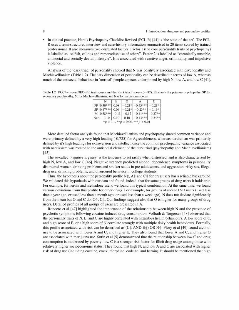
Analysis of the ‘dark triad’ of personality showed that N was positively associated with psychopathy andMachiavellianism (Table 1.2). The dark dimension of personality can be described in terms of low A, whereasmuch of the antisocial behaviour in ‘normal’ people appears underpinned by high N, low A, and low C [41].
Table 1.2 PCC between NEO-FFI trait scores and the ‘dark triad’ scores (n=82). PP stands for primary psychopathy, SP forsecondary psycholathy, M for Machiavellianism, and Nar for narcissism scores.
N E O A CPP 0.30*** 0.08 −0.21* −0.43*** −0.21*SP 0.47*** 0.04 −0.21* −0.23** −0.19*M 0.38*** −0.13 −0.17 −0.41*** −0.27**
Nar −0.10 0.10 0.10 −0.43*** −0.24***p < 0.1, **p < 0.05, ***p < 0.01
More detailed factor analysis found that Machiavellianism and psychopathy shared common variance andwere primary defined by a very high loading (-0.725) for Agreeableness, whereas narcissism was primarilydefined by it’s high loadings for extroversion and intellect, once the common psychopathic variance associatedwith narcissism was rotated to the antisocial element of the dark triad (psychopathy and Machiavellianism)[45].
The so-called ‘negative urgency’ is the tendency to act rashly when distressed, and is also characterized byhigh N, low A, and low C [46]. Negative urgency predicted alcohol dependence symptoms in personalitydisordered women, drinking problems and smoker status in pre-adolescents, and aggression, risky sex, illegaldrug use, drinking problems, and disordered behavior in college students.
Thus, the hypothesis about the personality profile N⇑, A⇓ and C⇓ for drug users has a reliable background.We validated this hypothesis with our data and found, indeed, that for some groups of drug users it holds true.For example, for heroin and methadone users, we found this typical combination. At the same time, we foundvarious deviations from this profile for other drugs. For example, for groups of recent LSD users (used lessthan a year ago, or used less than a month ago, or used less than a week ago), N does not deviate significantlyfrom the mean but O and C do: O⇑, C⇓. Our findings suggest also that O is higher for many groups of drugusers. Detailed profiles of all groups of users are presented in A.
Roncero et al [47] highlighted the importance of the relationship between high N and the presence ofpsychotic symptoms following cocaine-induced drug consumption. Vollrath & Torgersen [48] observed thatthe personality traits of N, E, and C are highly correlated with hazardous health behaviours. A low score of C,and high score of E, or a high score of N correlate strongly with multiple risky health behaviours. Formally,this profile associated with risk can be described as (C⇓ AND E⇑) OR N⇑. Flory et al [49] found alcoholuse to be associated with lower A and C, and higher E. They also found that lower A and C, and higher Oare associated with marijuana use. Sutin et al [5] demonstrated that the relationship between low C and drugconsumption is moderated by poverty; low C is a stronger risk factor for illicit drug usage among those withrelatively higher socioeconomic status. They found that high N, and low A and C are associated with higherrisk of drug use (including cocaine, crack, morphine, codeine, and heroin). It should be mentioned that high

1.4 The problem of the relationship between personality traits and drug consumption 9
N is positively associated with many other addictions like internet addiction, exercise addiction, compulsivebuying, and study addiction [50].
An individual’s personality profile contributes to becoming a drug user. Terracciano et al [51] demonstratedthat compared to ‘never smokers’, current cigarette smokers were lower on C and higher on N. They foundthat the profiles for cocaine and heroin users scored very high on N, and very low on C whilst marijuana usersscored high on O but low on A, and C. Turiano et al [52] found a positive correlation between N and O, anddrug use, while increasing scores for C and A decreases risk of drug use. Previous studies demonstrated thatparticipants who use drugs, including alcohol and nicotine, have a strong positive correlation between A and C,and a strong negative correlation for each of these factors with N [53, 54]. Three high-order personality traitsare proposed as endophenotypes for substance use disorders: Positive Emotionality, Negative Emotionality,and Constraint [55].
The problem of risk evaluation for individuals is much more complex. This was explored very recentlyby Yasnitskiy et al [56], Valeroa et al [80] and Bulut & Bucak [81]. Both individual and environmentalfactors predict substance use, and different patterns of interaction among these factors may have differentimplications [82]. Age is a very important attribute for diagnosis and prognosis of substance use disorders. Inparticular, early adolescent onset of substance use is a robust predictor of future substance use disorders [83].
Valeroa et al [80] evaluated the individual risk of drug consumption for alcohol, cocaine, opiates, cannabis,ecstasy, and amphetamines. Input data were collected using a Spanish version of the Zuckerman-KuhlmanPersonality Questionnaire (ZKPQ). Two samples were used in this study. The first one consisted of 336 drugdependent psychiatric patients of one hospital. The second sample included 486 control individuals. Theauthors used a decision tree as a tool to identify the most informative attributes. The sensitivity (proportion ofcorrectly identified positives) of 40% and specificity (proportion of correctly identified negatives) of 94% wereachieved for the training set. The main purpose of this research was to test if predicting drug consumption waspossible and to identify the most informative attributes using data mining methods. Decision tree methodswere applied to explore the differential role of personality profiles in drug consumer and control individuals.The two personality factors, Neuroticism and anxiety and the ZKPQ’s Impulsivity, were found to be mostrelevant for drug consumption prediction. The low sensitivity (40%) score means that such a decision treecannot be applied to real life situations.
Without focussing on specific addictions, Bulut & Bucak [81] estimated the proportion of teenagers whoexhibit a high risk of addiction. The attributes were collected by an original questionnaire, which included 25questions. The form was filled in by 671 students. The first 20 questions asked about the teenagers’ financialsituation, temperament type, family and social relations, and cultural preferences. The last five questions werecompleted by their teachers and concerned the grade point average of the student for the previous semesteraccording to a five-point grading system, whether the student had been given any disciplinary punishment sofar, if the student had alcohol problems, if the student smoked cigarettes or used tobacco products, and whetherthe student misused substances. In Bulut et al’s study there were five risk classes as outputs. The authorsdiagnosed teenagers’ risk of being a drug abuser using seven types of classification algorithms: k-nearestneighbor, ID3 and C4.5 decision tree based algorithms, naıve Bayes classifier, naıve Bayes/decision treeshybrid approach, one-attribute-rule, and projective adaptive resonance theory. The classification accuracy ofthe best classifier was reported as 98%.
Yasnitskiy et al [56], attempted to evaluate the individual’s risk of illicit drug consumption and torecommend the most efficient changes in the individual’s social environment to reduce this risk. The inputand output features were collected by an original questionnaire. The attributes consisted of: level of education,having friends who use drugs, temperament type, number of children in the family, financial situation, levels ofalcohol and cigarette smoking consumption, family relations (cases of physical, emotional and psychologicalabuse, level of trust and happiness in the family). There were 72 participants. A neural network model was
10 1 Introduction: drug use and personality profiles
used to evaluate the importance of attributes to diagnose the tendency towards drug addiction. A series ofvirtual experiments was performed for several test patients (drug users) to evaluate how possible it is tocontrol the propensity for drug addiction. The most effective change of social environment features waspredicted for each person. The recommended changes depended on the personal profile, and significantlyvaried for different participants. This approach produced individual bespoke advice to affect decreasing drugdependence.
Profiles of drug users have some similarity for all drugs (for example, N⇑ and C⇓), but substanceabuse populations differ in details and severity of these deviations form the normal profile. This importantobservation was done by Donovan et al. [57] in 1998. They used MMPI for personality description andanalysed groups of alcoholics, heroin, cocaine, and polydrug addicts by Discriminant Analysis. They identifiedthree functions in the MMPI data, which distinguished between the groups along important dimensions. Thesefunctions are: Level of Disturbance, Mania versus Alienated Depression, and Odd Thinking and Introversionversus Psychopathic Acting Out.
Two additional characteristics of personality are proven to be important for analysis of substance use,Impulsivity (Imp) and Sensation-Seeking (SS).
Imp Impulsivity is defined as a tendency to act without adequate forethought;SS Sensation-Seeking is defined by the search for experiences and feelings, that are varied, novel, complex
and intense, and by the readiness to take risks for the sake of such experiences.
It was shown that high SS is associated with increased risk of substance use [58–60].Imp has been operationalised in many different ways [61]. It was demonstrated that substance use disorders
are strongly associated with high personality trait Imp scores on various measures [62, 63]. Moreover, Impscore has significant impact on the treatment of substance use disorders: higher Imp implies lower successrate [63]. It is possible that psychosocial and pharamacological treatments that may decrease Imp will improvesubstance use treatment outcomes [63].
Impulsivity has been shown to predict aggression and heavy drinking [64]. Poor social problem solving hasbeen identified as a potential mediating variable between impulsivity and aggression. It is likely that the cog-nitive and behavioural features of impulsivity militate against the acquisition of good social problem-solvingskills early in life and that these deficits persist into adulthood, increasing the likelihood of interpersonalproblems.
A model was proposed, which attributes substance use/misuse to four distinct personality factors: SS, Imp,anxiety sensitivity (AS), and introversion/hopelessness (I/H). These four factors form a so-called SubstanceUse Risk Profile Scale [65]. The model was tested on groups of cannabis users [65–67]. It was demonstratedthat SS was positively associated with expansion motives, Imp was associated with drug availability motives,AS was associated with conformity motives and I/H was associated with coping motives for cannabis use [67].Therefore, the authors of this model concluded that four personality risk factors in the model are associatedwith distinct cannabis use motives.
The personality trait Imp and laboratory tests of neurobehavioral impulsivity measured different aspects ofgeneral impulsivity phenomenon. Relationships between these two aspects are different in groups of heroinusers and amphetamines users (even the sign of correlations is different) [68]. Very recently, demographic,personality (Imp, trait psychopathy, aggression, SS), psychiatric (attention deficit hyperactivity disorder,conduct disorder, antisocial personality disorder, psychopathy, anxiety, depression), and neurocognitiveimpulsivity measures (Delay Discounting, Go/No-Go, Stop Signal, Immediate Memory, Balloon AnalogueRisk, Cambridge Gambling, and Iowa Gambling tasks) are used as predictors in a machine-learning algorithmto separate 39 amphetamine mono-dependent, 44 heroin mono-dependent, 58 polysubstance dependent, and81 non-substance dependent individuals [69].
1.5 New dataset open for use 11
Two integrative personality dimensions capture important risk factors for substance use diorder [70]:
• Internalizing relates to generalized psychological distress, refers to insufficient amounts of behavior and issensitive to a wide range of problems in living (associated with overcontrol of emotion, social withdrawal,phobias, symptoms of depression, anxiety, somatic disorder, traumatic distress, suicide).
• Externalizing refers to acting-out problems that involve excess behavior and is often more directlyassociated with behaviors that cause distress for others, and to self as a consequence (associated withundercontrol of emotion, oppositional defiance, negativism, aggression, symptoms of attention deficit,hyperactivity, conduct, and other impulse control disorders).
Empirical results suggested co-occurrence of internalizing and externalizing problems among substanceusers [71]. Nevertheless, the externalizing dimension differentiated heroin users from alcohol, marijuana, andcocaine users [72]. Internalizing and externalizing symptoms can be evaluated in FFM [73].
Correlations between drug consumption and gender, age, family income and geographical location wasstudied in USA in a series of epidemiologic surveys (see [74]). For example, it was demonstrated that ratesof alcohol and cannabis abuse and dependence were greater among men than women. Nevertheless, thegender differences reported in large-scale epidemiological studies, were not pronounced in some adolescentsamples [75].
In our study [76, 77] we tested associations with personality traits and biographical data (age, gender, andeducation) for 18 different types of drugs separately, using the Revised NEO Five-Factor Inventory (NEO-FFI-R) [16], the Barratt Impulsiveness Scale Version 11 (BIS-11) [84], and the Impulsivity Sensation-SeekingScale (ImpSS) [85] to assess Imp and SS respectively. For this analysis, we employed various methods ofstatistics, data analysis and machine learning.
1.5 New dataset open for use
The database was collected by an anonymous online survey methodology by Elaine Fehrman, yielding2051 respondents. In January 2011, the research proposal was approved by the University of LeicesterForensic Psychology Ethical Advisory Group, and subsequently received strong support from the Universityof Leicester School of Psychology Research Ethics Committee (PREC).
The database is available online [78, 79]. An online survey tool from Survey Gizmo [86, 87] was employedto gather data which maximised anonymity; this was particularly relevant to canvassing respondents views,given the sensitive nature of drug use. All participants were required to declare themselves at least 18 years ofage prior to giving informed consent.
The study recruited 2051 participants over a 12-month recruitment period. Of these persons, 166 did notrespond correctly to a validity check built into the middle of the scale, so were presumed to be inattentive tothe questions being asked. Nine of these were also found to have endorsed the use of a fictitious drug, whichwas included precisely to identify respondents who overclaim, as have other studies of this kind [88]. This leda useable sample of 1885 participants (male/female = 943/942). It was found to be biased when comparedwith the general population, the comparison (see Chapter 3, Fig. 3.5) being based on the data published byEgan et al. [17] and Costa & McCrae [16]. Such a bias is usual for clinical cohorts [51, 99] and ‘problematic’or ‘pathological’ groups..
The sample recruited was highly educated, with just under two-thirds (59.5%) educated to, at least, degreeor professional certificate level: 14.4% (271) reported holding a professional certificate or diploma, 25.5%(481) an undergraduate degree, 15% (284) a master’s degree, and 4.7% (89) a doctorate. Approximately

12 1 Introduction: drug use and personality profiles
26.8% (506) of the sample had received some college or university tuition although they did not hold anycertificates; lastly, 13.6% (257) had left school at the age of 18 or younger.
Twelve attributes are known for each respondent: personality measurements which include N, E, O, A,and C scores from NEO-FFI-R, Impulsivity (Imp) from the BIS-11, Sensation Seeking (SS) from the ImpSS,level of education (Edu.), age, gender, country of residence, and ethnicity. The data set contains informationon the consumption of 18 central nervous system psychoactive drugs including alcohol, amphetamines, amylnitrite, benzodiazepines, cannabis, chocolate, cocaine, caffeine, crack, ecstasy, heroin, ketamine, legal highs,LSD, methadone, magic mushrooms (MMushrooms), nicotine, and Volatile Substance Abuse (VSA) i.e. glues,gases, and aerosols. One fictitious drug (Semeron) was introduced to identify overclaimers. For each drug,participants selected either: they never used this drug, used it over a decade ago, or in the last decade, year,month, week, or day.
Participants were asked about various substances, which were classified as either central nervous systemdepressants, stimulants, or hallucinogens. The depressant drugs comprised alcohol, amyl nitrite, benzodi-azepines, tranquilizers, solvents and inhalants, and opiates such as heroin and methadone/prescribed opiates.The stimulants consisted of amphetamines, nicotine, cocaine powder, crack cocaine, caffeine, and choco-late. Although chocolate contains caffeine, data for chocolate was measured separately, given that it mayinduce parallel psychopharmacological and behavioural effects in individuals congruent to other addictivesubstances [98]. The hallucinogens included cannabis, ecstasy, ketamine, LSD, and magic mushrooms. Legalhighs such as mephedrone, salvia, and various legal smoking mixtures were also measured.
The objective of the study was to assess the potential effect of the FFM personality traits, Imp, SS, anddemographic data on drug consumption for different drugs, groups of drugs and for different definitions of drugusers. The study had two purposes: (i) to identify the association of personality profiles (i.e. FFM+Imp+SS)with drug consumption and (ii) to predict the risk of drug consumption for each individual according to theirpersonality profile.
Participants were asked to indicate which ethnic category was broadly representative of their culturalbackground. An overwhelming majority (91.2%; 1720) reported being White, (1.8%; 33) stated they wereBlack, and (1.4%; 26) Asian. The remainder of the sample (5.6%; 106) described themselves as ‘Other’ or‘Mixed’ categories. This small number of persons belonging to specific non-white ethnicities precluded anyanalyses involving racial categories.
In order to assess the personality traits of the sample, the Revised NEO Five-Factor Inventory (NEO-FFI-R)questionnaire was employed [11]. The NEO-FFI-R is a highly reliable measure of basic personality domains;internal consistencies are 0.84 (N); 0.78 (E); 0.78 (O); 0.77 (A), and 0.75 (C) [89]. The scale is a 60-iteminventory comprised of five personality domains or factors. The NEO-FFI-R is a shortened version of theRevised NEO-Personality Inventory (NEO-PI-R) [11]. The five factors are: N, E, O, A, and C with 12 itemsper domain.
All of these domains are hierarchically defined by specific facets [90]. Egan et al. [17] observed thatthe score for the O and E domains of the NEO-FFI instrument are less reliable than for N, A, and C. Thepersonality traits are not independent. They are correlated, with higher N being associated with lower E, lowerA and lower C, and higher E being associated with higher C (see Table 1.3 for more details).
In our study, participants were asked to read the 60 NEO-FFI-R statements and indicate on a five-pointLikert–type scale how much a given item applied to them (i.e. 0 = ‘Strongly Disagree’, 1 = ‘Disagree’, 2 =‘Neutral’, 3 = ‘Agree’, to 4 = ‘Strongly Agree’).
The second measure used was the Barratt Impulsiveness Scale (BIS-11) [84]. BIS-11 is a 30-item self-reportquestionnaire, which measures the behavioural construct of impulsiveness, and comprises three subscales:motor impulsiveness, attentional impulsiveness, and non-planning. The ‘motor’ aspect reflects acting withoutthinking, the ‘attentional’ component, poor concentration and thought intrusions, and the ‘non-planning’, a

1.5 New dataset open for use 13
Table 1.3 Pearson’s correlation coefficients (PCC) between NEO-FFI trait scores for a large British sample, n = 1025 [17]; thep-value is the probability of observing by chance the same or greater correlation coefficient if the data are uncorrelated
N E O A CN −0.40** 0.07* −0.22** −0.36**E −0.40** 0.16** 0.22** 0.30**O 0.07* 0.16** 0.08* −0.15**A −0.22** 0.22** 0.08* 0.13**C −0.36** 0.30* −0.15** 0.13**
∗p < 0.02, **p < 0.001
lack of consideration for consequences [91]. The scale’s items are scored on a four-point Likert-type scale.This study modified the response range to make it compatible with previous related studies [92]. A score offive usually connotes the most impulsive response although some items are reverse-scored to prevent responsebias. Items are aggregated, and the higher the BIS-11 scores are, the higher the impulsivity level [93] is.BIS-11 is regarded a reliable psychometric instrument with good test-retest reliability (Spearman’s rho isequal to 0.83) and internal consistency (Cronbach’s alpha is equal to 0.83 [84, 91]).
The third measurement tool employed was the Impulsiveness Sensation-Seeking (ImpSS). Although theImpSS combines the traits of impulsivity and sensation-seeking, it is regarded as a measure of a generalsensation-seeking trait [85]. The scale consists of 19 statements in true-false format, comprising eight itemsmeasuring impulsivity (Imp), and 11 items gauging Sensation-Seeking (SS). The ImpSS is considered a validand reliable measure of high risk behavioural correlates such as substance misuse [94].
It was recognised at the outset of this study that drug use research regularly (and spuriously) dichotomisesindividuals as users or non-users, without due regard to their frequency or duration/desistance of drug use [95].In this study, finer distinctions concerning the measurement of drug use have been deployed, due to thepotential for the existence of qualitative differences amongst individuals with varying usage levels. In relationto each drug, respondents were asked to indicate if they never used this drug, used it over a decade ago, or inthe last decade, year, month, week, or day. This format captured the breadth of a drug-using career, and thespecific recency of use.
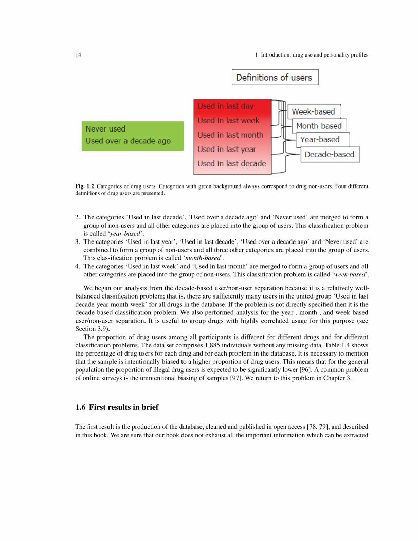
For decade based separation, we merged two isolated categories (‘Never used’ and ‘Used over a decadeago’) into the class of non-users, and all other categories were merged to form the class of users. For year-based classification we additionally merged the category ‘Used over a decade ago’ into the group of non-usersand placed four other categories (‘Used in last year-month-week-day’) into the group of users. We continuedseparating into users and non-users depending on the timescale in this nested “Russian doll” style. We alsoconsidered ‘month-based’ and ‘week-based’ user/non-user separations. Different categories of drug users aredepicted in Fig 1.2.
Analysis of the classes of drug users shows that part of the classes are nested: participants which belongto the category ‘Used in last day’ also belong to the categories ‘Used in last week’, ‘Used in last month’,‘Used in last year’ and ‘Used in last decade’. There are two special categories: ‘Never used’ and ‘Used over adecade ago’ (see Fig 1.2). The data does not contain a definition of the users and non-users groups. Formallyonly a participant in the class ‘Never used’ can be called a non-user, but a participant who used a drug morethan decade ago also cannot be considered a drug user for most applications. There are several possible waysto discriminate participants into groups of users and non-users for binary classification:
1. Two isolated categories (‘Never used’ and ‘Used over a decade ago’) are placed into the class of non-userswith a green background in Fig 1.2, and all other categories into the class ‘users’ as the simplest version ofbinary classification. This classification problem is called ‘decade-based’ user/non-user separation.
14 1 Introduction: drug use and personality profiles
Fig. 1.2 Categories of drug users. Categories with green background always correspond to drug non-users. Four differentdefinitions of drug users are presented.
2. The categories ‘Used in last decade’, ‘Used over a decade ago’ and ‘Never used’ are merged to form agroup of non-users and all other categories are placed into the group of users. This classification problemis called ‘year-based’.
3. The categories ‘Used in last year’, ‘Used in last decade’, ‘Used over a decade ago’ and ‘Never used’ arecombined to form a group of non-users and all three other categories are placed into the group of users.This classification problem is called ‘month-based’.
4. The categories ‘Used in last week’ and ‘Used in last month’ are merged to form a group of users and allother categories are placed into the group of non-users. This classification problem is called ‘week-based’.
We began our analysis from the decade-based user/non-user separation because it is a relatively well-balanced classification problem; that is, there are sufficiently many users in the united group ‘Used in lastdecade-year-month-week’ for all drugs in the database. If the problem is not directly specified then it is thedecade-based classification problem. We also performed analysis for the year-, month-, and week-baseduser/non-user separation. It is useful to group drugs with highly correlated usage for this purpose (seeSection 3.9).
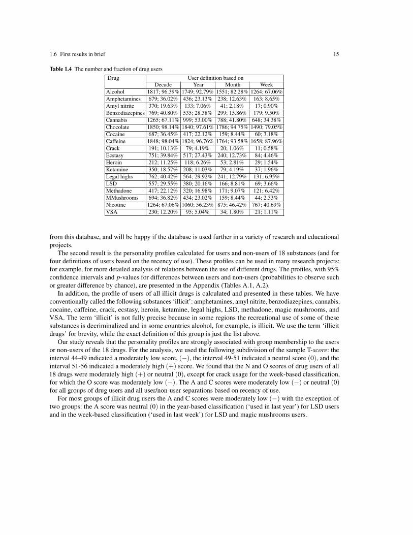
The proportion of drug users among all participants is different for different drugs and for differentclassification problems. The data set comprises 1,885 individuals without any missing data. Table 1.4 showsthe percentage of drug users for each drug and for each problem in the database. It is necessary to mentionthat the sample is intentionally biased to a higher proportion of drug users. This means that for the generalpopulation the proportion of illegal drug users is expected to be significantly lower [96]. A common problemof online surveys is the unintentional biasing of samples [97]. We return to this problem in Chapter 3.
1.6 First results in brief
The first result is the production of the database, cleaned and published in open access [78, 79], and describedin this book. We are sure that our book does not exhaust all the important information which can be extracted
1.6 First results in brief 15
Table 1.4 The number and fraction of drug users
Drug User definition based onDecade Year Month Week
Alcohol 1817; 96.39% 1749; 92.79% 1551; 82.28% 1264; 67.06%Amphetamines 679; 36.02% 436; 23.13% 238; 12.63% 163; 8.65%Amyl nitrite 370; 19.63% 133; 7.06% 41; 2.18% 17; 0.90%Benzodiazepines 769; 40.80% 535; 28.38% 299; 15.86% 179; 9.50%Cannabis 1265; 67.11% 999; 53.00% 788; 41.80% 648; 34.38%Chocolate 1850; 98.14% 1840; 97.61% 1786; 94.75% 1490; 79.05%Cocaine 687; 36.45% 417; 22.12% 159; 8.44% 60; 3.18%Caffeine 1848; 98.04% 1824; 96.76% 1764; 93.58% 1658; 87.96%Crack 191; 10.13% 79; 4.19% 20; 1.06% 11; 0.58%Ecstasy 751; 39.84% 517; 27.43% 240; 12.73% 84; 4.46%Heroin 212; 11.25% 118; 6.26% 53; 2.81% 29; 1.54%Ketamine 350; 18.57% 208; 11.03% 79; 4.19% 37; 1.96%Legal highs 762; 40.42% 564; 29.92% 241; 12.79% 131; 6.95%LSD 557; 29.55% 380; 20.16% 166; 8.81% 69; 3.66%Methadone 417; 22.12% 320; 16.98% 171; 9.07% 121; 6.42%MMushrooms 694; 36.82% 434; 23.02% 159; 8.44% 44; 2.33%Nicotine 1264; 67.06% 1060; 56.23% 875; 46.42% 767; 40.69%VSA 230; 12.20% 95; 5.04% 34; 1.80% 21; 1.11%
from this database, and will be happy if the database is used further in a variety of research and educationalprojects.
The second result is the personality profiles calculated for users and non-users of 18 substances (and forfour definitions of users based on the recency of use). These profiles can be used in many research projects;for example, for more detailed analysis of relations between the use of different drugs. The profiles, with 95%confidence intervals and p-values for differences between users and non-users (probabilities to observe suchor greater difference by chance), are presented in the Appendix (Tables A.1, A.2).
In addition, the profile of users of all illicit drugs is calculated and presented in these tables. We haveconventionally called the following substances ‘illicit’: amphetamines, amyl nitrite, benzodiazepines, cannabis,cocaine, caffeine, crack, ecstasy, heroin, ketamine, legal highs, LSD, methadone, magic mushrooms, andVSA. The term ‘illicit’ is not fully precise because in some regions the recreational use of some of thesesubstances is decriminalized and in some countries alcohol, for example, is illicit. We use the term ‘illicitdrugs’ for brevity, while the exact definition of this group is just the list above.
Our study reveals that the personality profiles are strongly associated with group membership to the usersor non-users of the 18 drugs. For the analysis, we used the following subdivision of the sample T-score: theinterval 44-49 indicated a moderately low score, (−), the interval 49-51 indicated a neutral score (0), and theinterval 51-56 indicated a moderately high (+) score. We found that the N and O scores of drug users of all18 drugs were moderately high (+) or neutral (0), except for crack usage for the week-based classification,for which the O score was moderately low (−). The A and C scores were moderately low (−) or neutral (0)for all groups of drug users and all user/non-user separations based on recency of use.
For most groups of illicit drug users the A and C scores were moderately low (−) with the exception oftwo groups: the A score was neutral (0) in the year-based classification (‘used in last year’) for LSD usersand in the week-based classification (‘used in last week’) for LSD and magic mushrooms users.
16 1 Introduction: drug use and personality profiles
The A and C scores for groups of legal drugs users (i.e. alcohol, chocolate, caffeine, and nicotine)were neutral (0), apart from nicotine users, whose C score was moderately low (−) for all categories ofuser/non-user separation.
The impact of the E score was drug specific. For example, for the week-based user/non-user separation theE scores were:
• moderately low (−) for amphetamines, amyl nitrite, benzodiazepines, heroin, ketamine, legal highs,methadone, and crack;
• moderately high (+) for cocaine, ecstasy, LSD, magic mushrooms, and VSA;• neutral (0) for alcohol, caffeine, chocolate, cannabis, and nicotine.
For more details see Section 3.5.Usage of some drugs were correlated significantly. The structure of these correlations is analysed in Section
3.6. Two correlation measures were utilised: the Pearson’s Correlation Coefficient (PCC) and the RelativeInformation Gain (RIG). We found three groups of drugs with highly correlated use (Section 3.9). Thecentral element was clearly identified for each group. These centres are: heroin, ecstasy, and benzodiazepines.This means that drug consumption has a ‘modular structure’, which is made clear in the correlation graph.The idea of merging correlated attributes into ‘modules’ referred to as correlation pleiades is popular inbiology [100–102].
The concept of correlation pleiades was introduced in biostatistics in 1931 [100]. They were used foridentification of a modular structure in evolutionary physiology [100–103]. According to Berg [102], correla-tion pleiades are clusters of correlated traits. In our approach, we distinguished the core and the peripheralelements of correlation pleiades and allowed different pleiades to have small intersections in their periphery.‘Soft’ clustering algorithms relax the restriction that each data object is assigned to only one cluster (likeprobabilistic [104] or fuzzy [105] clustering). See the book of R. Xu & D. Wunsch [106] for a modern reviewof hard and soft clustering. We refer to [107] for a discussion of clustering in graphs with intersections.
The three groups of correlated drugs centered around heroin, ecstasy, and benzodiazepines were definedfor the decade-, year-, month-, and week-based classifications:
• The heroin pleiad includes crack, cocaine, methadone, and heroin;• The ecstasy pleiad consists of amphetamines, cannabis, cocaine, ketamine, LSD, magic mushrooms, legal
highs, and ecstasy;• The benzodiazepines pleiad contains methadone, amphetamines, cocaine, and benzodiazepines.
The topology of the correlation graph can help in analysis of mini-sequences of drug involvement. Thesemini-sequences can be found in longitudinal studies [108]: cigarettes are a gateway to cannabis, and then tohard drugs; and there is a synergistic effect of increasing involvement. Of course, correlation does not imply acausal relationship, but use of the substances from one mini-sequence of involvement should be correlated.Therefore, the correlation graph is a proper map for the study of the involvement routes, and synergistic andreciprocal effects.
Analysis of the intersections between correlation pleiades of drugs leads to important questions andhypotheses:
• Why is cocaine a peripheral member of all pleiades?• Why does methadone belong to the periphery of both the heroin and benzodiazepines pleiades?• Do these intersections reflect the structure of individual drug consumption and sequences of involvement,
or are they related to the structure of the groups of drug consumers?

1.6 First results in brief 17
In this study, we evaluated the individual drug consumption risk separately, for each drug and pleiad ofdrugs. We also analysed interrelations between the individual drug consumption risks for different drugs. Weapplied several data mining approaches: decision tree, random forest, k-nearest neighbours, linear discriminantanalysis, Gaussian mixture, probability density function estimation, logistic regression and naıve Bayes.The quality of classification was surprisingly high (Section 3.8). We tested all of the classifiers by Leave-One-Out Cross Validation. The best results, with sensitivity and specificity greater than 75%, were achievedfor cannabis, crack, ecstasy, legal highs, LSD, and VSA. Sensitivity and specificity greater than 70% wereachieved for the following drugs: amphetamines, amyl nitrite, benzodiazepines, chocolate, caffeine, heroin,ketamine, methadone and nicotine. An exhaustive search was performed to select the most effective subset ofinput features and data mining methods for each drug. The results of this analysis provide an answer to animportant question about the predictability of drug consumption risk on the basis of FFM+Imp+SS profileand demographic data.
Users for each correlation pleiad of drugs are defined as users of any of the drugs from the pleiad. We solvedthe classification problem for drug pleiades for the decade-, year-, month-, and week-based user/non-userseparations. The quality of classification is also high.
Simple Fisher’s linear discriminant classifiers have slightly worse performance than more advanced ma-chine learning methods but are very robust, and give additional information. Coefficients of the discriminantsare presented in the Appendix for all user/non-user separation problems for every substance, group of illicitsubstances, and three correlation pleiades. Stability of the discriminant models was tested in cross-validation.Even a brief look at the linear discriminants reveals differences between drugs. For example, for month-baseduser definition (‘used in last month’), the linear discriminants for heroin and cocaine users for seven variablesFFM+Imp+SS are (Table A.15):
heroin users −30.020+0.302N−0.409E+0.232O−0.499A−0.107C+0.345Imp+0.555SS > 0;cocaine users −57.737+0.366N+0.148E+0.082O−0.370A−0.014C−0.001Imp+0.837SS > 0,
where the variables are represented by their T-scores (calculated for the database). These data, together withthe correlation tables (Tables A.3, A.4), give information about the importance of different variables foruser/non-user separation for different drugs.
We also studied the problem of separation of users of different drugs. For this purpose, we selected threedrugs: heroin, ecstasy, and benzodiazepines (the centres of the pleiades). The profiles of the users of thesedrugs are different (see Fig. 3.21) (the confidence level below is 95%):
• The mean values in the groups of benzodiazepines and ecstasy users are statistically significantly differentfor N (higher for benzodiazepines) and E (higher for ecstasy) for all definitions of users, for O (higherfor ecstasy) for all definitions of users excluding the year-based, and for SS (higher for ecstasy) for alldefinitions excluding the month-based.
• The groups of benzodiazepines and heroin users are statistically significantly different for A (higher forbenzodiazepines) for all definitions of users, for Imp (higher for heroin) and SS (higher for heroin) for alldefinitions of users excluding the week-based.
• Heroin and ecstasy are statistically significantly different for N (higher for heroin), E (higher for ecstasy)and A (higher for ecstasy) for all definitions of users and for Imp (higher for heroin) for all definitionsexcluding the week-based.
The creation of classifiers has provided the ability to evaluate the risk of drug consumption in relationto individuals. The risk map is a useful tool for data visualisation and for the generation of hypotheses forfurther study (see Chapter ‘Risk evaluation for the decade-based user/non-user separation’).

18 1 Introduction: drug use and personality profiles
In the next chapter, we briefly introduce the main methods used in the book, in Chapter 3 the results aredescribed in more detail, then after a brief Discussion and Summary, the main tables are presented in theAppendix.
References
1. Kleiman, M.A., Caulkins, J.P., Hawken, A.: Drugs and Drug Policy: What Everyone Needs to Know. Oxford UniversityPress, New York (2011)
2. Beaglehole, R., Bonita, R., Horton, R., Adams, C., Alleyne, G., Asaria, P., Baugh, V., Bekedam, H., Billo, N., CasswellS., Cecchini, M., Colagiuri, R., Colagiuri, S., Collins, T., Ebrahim, S., Engelgau, M., Galea, G., Gaziano, T., Geneau, R.,Haines, A., Hospedales, J., Jha, P., Keeling, A., Leeder, S., Lincoln, P., McKee, M., Mackay, J., Magnusson, R., Moodie,R., Mwatsama, M., Nishtar, S., Norrving, B., Patterson, D., Piot, P., Ralston, J., Rani, M., Reddy, K.S., Sassi, F., Sheron,N., Stuckler, D., Suh, I., Torode, J., Varghese, C., Watt, J.: Priority actions for the non-communicable disease crisis. Lancet377(9775), 1438–1447 (2011). doi:10.1016/S0140-6736(11)60393-0
3. Bickel, W.K., Johnson, M.W., Koffarnus, M.N., MacKillop, J., Murphy, J.G.: The behavioral economics of substance use dis-orders: reinforcement pathologies and their repair. Annu. Rev. Clin. Psychol. 10(1), 641–677 (2014). doi:10.1146/annurev-clinpsy-032813-153724
4. McGinnis, J.M., Foege, W.H.: Actual causes of death in the United States. JAMA (J. Am. Med. Assoc.) 270(18), 2207–2212(1993) doi:10.1001/jama.1993.03510180077038
5. Sutin, A.R., Evans, M.K., Zonderman, A.B.: Personality traits and illicit substances: the moderation role of poverty. DrugAlcohol Depend. 131(3), 247–251 (2013). doi:10.1016/j.drugalcdep.2012.10.020
6. American Psychiatric Association: Diagnostic and Statistical Manual of Mental Disorders (DSM-5)https://www.psychiatry.org/psychiatrists/practice/dsm (2013) Accessed 27 Dec 2017
7. World Health Organization, Geneva: Prevention of mental disorders: effective interventions and policy options: summaryreport. http://www.who.int/mental health/evidence/en/prevention of mental disorders sr.pdf (2004) Accessed 27 Dec 2017
8. Goldberg, L.R.: The structure of phenotypic personality traits. Am. psychol. 48(1), 26–34 (1993). doi:10.1037//0003-066x.48.1.26
9. Thurstone, L.L.: The vectors of mind. Psychol. Rev. 41(1), 1–32 (1934). doi:10.1037/h007595910. Digman, J.M.: Personality structure: Emergence of the five-factor model. Annu. Rev. Psychol. 41(1), 417–440 (1990).
doi:10.1146/annurev.psych.41.1.41711. Costa, P.T., MacCrae, R.R.: Revised NEO-personality inventory (NEO PI-R) and NEO five-factor inventory (NEO FFI):
Professional manual. Psychological Assessment Resources, Odessa, FL (1992)12. McCrae, R.R., John, O.P.: An introduction to the five-factor model and its applications. J. Pers. 60(2), 175–215 (1992).
doi:10.1111/j.1467-6494.1992.tb00970.x13. Poropat, A.E.: A meta-analysis of the five-factor model of personality and academic performance. Psychol. Bull. 135(2),
322–338 (2009). doi:10.1037/a001499614. Seibert, S.E., Kraimer, M.L.: The five-factor model of personality and career success. J. Vocat. Behav. 58(1), 1–21 (2001).
doi:10.1006/jvbe.2000.175715. Mount, M.K., Barrick, M.R., Stewart, G.L.: Five-factor model of personality and performance in jobs involving interpersonal
interactions. Hum. Perform. 11(2-3), 145–165 (1998). doi:10.1080/08959285.1998.966802916. McCrae, R.R., Costa, P.T.: A contemplated revision of the NEO five-factor inventory. Personal. Individ. Differ. 36(3),
587–596 (2004). doi:10.1016/s0191-8869(03)00118-117. Egan, V., Deary, I., Austin, E.: The NEO-FFI: Emerging British norms and an item-level analysis suggest N, A and C are
more reliable than O and E. Personal. Individ. Differ. 29(5), 907–920 (2000). doi:10.1016/s0191-8869(99)00242-118. Bagby, R.M., Costa, P.T., Widiger, T.A., Ryder, A.G., Marshall, M.: DSM-IV personality disorders and the Five-Factor
Model of personality: a multi-method examination of domain- and facet-level predictions. Eur. J. Personal. 19(4), 307–324(2005). doi:10.1002/per.563
19. Dorrer, M.G., Gorban, A.N., Kopytov, A.G., Zenkin, V.I.: Psychological intuition of neural networks. In: DeWitt, J.T.(ed.): Proceedings of the WCNN’95 (World Congress on Neural Networks’95, Washington DC, July 1995), pp. 193–196.Lawrence Erlbaum Associate (1996)
20. Gorban, A.N., Rossiyev, D.A., Butakova, E.V., Gilev, S.E., Golovenkin, S.E., Dogadin, S.A., Kochenov, D.A., Maslennikova,E.V., Matyushin, G.V., Mirkes, E.M., Nazarov, B.V.: Medical and physiological applications of MultiNeuron neural

References 19
simulator. In: DeWitt, J.T. (ed.): Proceedings of the WCNN’95 (World Congress on Neural Networks’95, Washington DC,July 1995), pp. 170–175. Lawrence Erlbaum Associate (1996).
21. Cleveland, M.J., Feinberg, M.E., Bontempo, D.E., Greenberg, M.T.: The role of risk and protective factors in substance useacross adolescence. J. Adolesc. Health 43(2), 157–164 (2008). doi:10.1016/j.jadohealth.2008.01.015
22. Ventura, C.A., de Souza, J., Hayashida, M., Ferreira, P.S.: Risk factors for involvement with illegal drugs: opinion of familymembers or significant others. J. Subst. Use 20(2), 136–142 (2014). doi:10.3109/14659891.2013.875077
23. McGue, M., Elkins, I., Iacono, W.G.: Genetic and environmental influences on adolescent substance use and abuse. Am. J.Med. Genet. Part A. 96(5), 671–677 (2000). doi:10.1002/1096-8628(20001009)96:5%3C671::aid-ajmg14%3E3.0.co;2-w
24. Dubey, C., Arora, M., Gupta, S., Kumar, B.: Five factor correlates: A comparison of substance abusers and non-substanceabusers. J. Indian Acad. Appl. Psychol. 36(1), 107–114 (2010)
25. Bogg, T., Roberts, B.W.: Conscientiousness and health-related behaviors: A meta-analysis of the leading behavioralcontributors to mortality. Psychol. Bull. 130(6), 887–919 (2004). doi:10.1037/0033-2909.130.6.887
26. Khantzian, E.J., Khantzian, N.J.: Cocaine addiction: is there a psychological predisposition? Psychiatr. Ann. 14(10),753–759 (1984). doi:10.3928/0048-5713-19841001-11
27. Steyer, R., Mayer, A., Geiser, C., Cole, D.A. A theory of states and traits – Revised. Annu. Rev. Clin. Psychol. 11, 7198(2015). doi:10.1146/annurev-clinpsy-032813-153719
28. McCrae, R.R., Costa, P.T.: Self-concept and the stability of personality: cross-sectional comparisons of self-reports andratings. J. Personal. Soc. Psychol. 43(6), 1282–1292 (1982). doi:10.1037/0022-3514.43.6.1282
29. McCrae, R.R., Costa, P.T.: The stability of personality: observations and evaluations. Curr. Dir. Psychol. Sci. 3(6), 173–175(1994). doi:10.1111/1467-8721.ep10770693
30. Heatherton, T.F., Weinberger, J.L. (eds.): Can personality change? American Psychological Association, Washington, DC,US (1994). doi:10.1037/10143-000
31. Schmitt, D. P., Allik, J., McCrae, R. R., Benet-Martnez, V.: The geographic distribution of Big Five personality traits:Patterns and profiles of human self-description across 56 nations. J. Cross-Cult. Psychol. 38(2), 173–212 (2007).http://doi:10.1177/0022022106297299
32. Costa, P.T., McCrae, R.R.: Set like plaster? Evidence for the stability of adult personality. In: Heatherton, T.F. , Weinberger,J.L. (eds.): Can personality change? pp. 21–40. American Psychological Association, Washington, DC, US (1994).doi:10.1037/10143-002
33. Weinberger, J.L.: Can personality change? In: Heatherton, T.F., Weinberger, J.L. (eds.) Can personality change? pp.333–350. American Psychological Association, Washington, DC, US (1994). doi:10.1037/10143-013
34. Carter, J.A., Herbst, J.H., Stoller, K.B., King, V., Kidorf, M.S., Costa, P.T., Brooner, R.K.: Short-term stability of NEO-PI-Rpersonality trait scores in opioid-dependent outpatients. Psychol. Addict. Behav. 15, 255–260 (2001). doi:10.1037//0893-164x.15.3.255
35. Widiger, T.A., Trull, T.J., Clarkin, J.F., Sanderson, C., Costa, P.T.: A description of the DSM-IV personality disorders withthe five-factor model of personality. In: Costa, P.T., Widiger, T.A. (eds.) Personality disorders and the five-factor model ofpersonality, 2nd edn. pp. 89–99. American Psychological Association, Washington, DC, US (2002). doi:10.1037/10423-006
36. De Fruyt, F., Van Leeuwen, K., Bagby, R. M., Rolland, J.-P., Rouillon, F.: (2006) Assessing and interpreting personalitychange and continuity in patients treated for major depression. Psychol. Assess. 18(1), 71–80 (2006). doi:10.1037/1040-3590.18.1.71
37. Kotov, R., Gamez, W., Schmidt, F., Watson, D.: Linking big personality traits to anxiety, depressive, and substance usedisorders: A meta-analysis. Psychol. bull. 136(5), 768–821 (2010). doi:10.1037/a0020327
38. Brooner, R.K., Schmidt, C.W., Herbst, J.H.: Personality trait characteristics of opioid abusers with and without comorbidpersonality disorders. In: Costa, P.T., Widiger, T.A. (eds.) Personality disorders and the five-factor model of personality. pp.131–148. American Psychological Association, Washington, DC, US (1994) doi:10.1037/10140-025
39. Kornør, H., Nordvik, H.: Five-factor model personality traits in opioid dependence. BMC Psychiatr. 7(1), 7 (2007).doi:10.1186/1471-244x-7-37
40. McCormick, R.A., Dowd, E.R., Quirt, S., Zegarra, J.H.: The relationship of NEO-PI performance to coping styles,patterns of use, and triggers for use among substance abusers. Addict. Behav. 23(4), 497–507 (1998). doi:10.1016/s0306-4603(98)00005-7
41. Jakobwitz, S., Egan, V.: The dark triad and normal personality traits. Personal. Individ. Differ. 40(2), 331–339 (2006).doi:10.1016/j.paid.2005.07.006
42. McHoskey, J.W., Worzel, W., Szyarto, C.: Machiavellianism and psychopathy. J. Personal. Soc. Psychol. 74(1), 192–210(1998). doi:10.1037//0022-3514.74.1.192
43. Raskin, R.N., Hall, C.S.: A narcissistic personality inventory. Psychological reports. 45(2), 590–590 (1979).doi:10.2466/pr0.1979.45.2.590
44. Hare, R.D.: Manual for the Revised Psychopathy Checklist. Multi-Health Systems, Toronto, ON (2003).

20 1 Introduction: drug use and personality profiles
45. Egan, V., Chan, S., Shorter, G. W.: The Dark Triad, happiness and subjective well-being. Pers. Individ. Differ. 67, 17–22(2014). doi:10.1016/j.paid.2014.01.004
46. Settles, R.E., Fischer, S., Cyders, M.A., Combs, J.L., Gunn, R.L., Smith G.T.: Negative urgency: a personality predictor ofexternalizing behavior characterized by neuroticism, low conscientiousness, and disagreeableness. J. Abnorm. Psychol.121(1), 160–172 (2012). doi:10.1037/a0024948
47. Roncero, C., Daigre, C., Barral, C., Ros-Cucurull, E., Grau-Lopez, L., Rodrıguez-Cintas, L., Tarifa, N., Casas, M., Valero,S.: Neuroticism associated with cocaine-induced psychosis in cocaine-dependent patients: a cross-sectional observationalstudy. PloS one. 9(9), e106111 (2014). doi:10.1371/journal.pone.0106111
48. Vollrath, M., Torgersen, S.: Who takes health risks? a probe into eight personality types. Personal. Individ. Differ. 32(7),1185–1197 (2002). doi:10.1016/s0191-8869(01)00080-0
49. Flory, K., Lynam, D., Milich, R., Leukefeld, C., Clayton, R.: The relations among personality, symptoms of alcohol and mar-ijuana abuse, and symptoms of comorbid psychopathology: results from a community sample. Exp. Clin. Psychopharmacol.10(4), 425–434 (2002). doi:10.1037//1064-1297.10.4.425
50. Andreassen, C.S., Griffiths, M.D., Gjertsen, S.R., Krossbakken, E., Kvam, S., Pallesen, S.: The relationships between behav-ioral addictions and the five-factor model of personality. J. Behav. Addict. 2(2), 90–99 (2013). doi:10.1556/jba.2.2013.003
51. Terracciano, A., Lockenhoff, C.E., Crum, R.M., Bienvenu, O.J., Costa, P.T.: Five-factor model personality profiles of drugusers. BMC Psychiatr. 8(1), 22 (2008). doi:10.1186/1471-244x-8-22
52. Turiano, N.A., Whiteman, S.D., Hampson, S.E., Roberts, B.W., Mroczek, D.K.: Personality and substance use inmidlife: Conscientiousness as a moderator and the effects of trait change. J. Res. Personal. 46(3), 295–305 (2012).doi:10.1016/j.jrp.2012.02.009
53. Stewart, S.H., Devine, H.: Relations between personality and drinking motives in young adults. Personal. Individ. Differ.29(3), 495–511 (2000). doi:10.1016/s0191-8869(99)00210-x
54. Haider, A.H., Edwin, D.H., MacKenzie, E.J., Bosse, M.J., Castillo, R.C., Travison, T.G., LEAP Study Group: The use ofthe NEO-five factor inventory to assess personality in trauma patients: a two-year prospective study. J. Orthop. Trauma16(9), 660–667 (2002). doi:10.1097/01.BOT.0000031328.88511.BF
55. Belcher, A.M., Volkow, N.D., Moeller, F.G., Ferre, S.: Personality traits and vulnerability or resilience to substance usedisorders. Trends cogn. sci. 18(4), 211–217 (2016). doi:10.1016/j.tics.2014.01.010
56. Yasnitskiy, L.N., Gratsilev, V.I., Kulyashova, J.S., Cherepanov F.M.: Possibilities of artificial intellect in detection ofpredisposition to drug addiction. Perm Univ. Her. Ser. “Philos. Psychol. Sociol.” 1(21), 61–73 (2015)
57. Donovan, J.M., Soldz, S., Kelley, H.F., Penk, W.E.: Four addictions: the MMPI and discriminant function analysis. J.Addict. Dis. 17(2), 41–55 (1998). doi:10.1300/j069v17n02 04
58. Zuckerman, M., Bone, R. N., Neary, R., Mangelsdorff, D., Brustman, B.: What is the sensation seeker? Personal-ity trait and experience correlates of the Sensation-Seeking Scales. J. Consult. Clin. Psychol. 39(2), 308–321 (1972).doi:10.1037/h0033398
59. Liraud, F., Verdoux, H.: 2000. Which temperamental characteristics are associated with substance use in subjects withpsychotic and mood disorders? Psychiatr. Res. 93, 63–72. doi:10.1016/s0165-1781(99)00120-1
60. Kopstein, A.N., Crum, R.M., Celentano, D.D., Martin, S.S.: Sensation seeking needs among 8th and 11th graders: charac-teristics associated with cigarette and marijuana use. Drug Alcohol Depend. 62(3), 195–203 (2001). doi:10.1016/s0376-8716(00)00170-8
61. Evanden, J.L.: Varieties of impulsivity. Psychopharmacol. 146(4), 348–61 (1999). doi:10.1007/pl0000548162. Verdejo-Garcia, A., Lawrence, A.J., Clark, L.: Impulsivity as a vulnerability marker for substance-use disorders: review of
findings from high-risk research, problem gamblers and genetic association studies. Neurosci. Biobehav. Rev. 32, 777–810(2008). doi:10.1016/j.neubiorev.2007.11.003
63. Loree, A.M., Lundahl, L.H., Ledgerwood, D.M.: Impulsivity as a predictor of treatment outcome in substance use disorders:review and synthesis. Drug Alcohol Rev. 34(2), 119–134 (2015). doi:10.1111/dar.12132
64. McMurran, M., Blair, M., Egan, V.: An investigation of the correlations between aggression, impulsiveness, socialproblemsolving, and alcohol use. Aggress. Behav. 28(6), 439–445 (2002). doi:10.1002/ab.80017
65. Conrod, P.J., Pihl, R.O., Stewart, S.H., Dongier, M.: Validation of a system of classifying female substance abusers on thebasis of personality and motivational risk factors for substance abuse. Psychol. Addict. Behav. 14(3), 243–256 (2000).doi:10.1037//0893-164x.14.3.243
66. Woicik, P.A., Stewart, S.H., Pihl, R.O., Conrod, P.J.: The substance use risk profile scale: A scale measuring traits linked toreinforcement-specific substance use profiles. Addict. Behav. 34(12), 1042–1055 (2009). doi:10.1016/j.addbeh.2009.07.001
67. Hecimovic, K., Barrett, S.P., Darredeau, C., Stewart, S.H.: Cannabis use motives and personality risk factors. Addict.Behav. 39(3), 729–732 (2014). doi:10.1016/j.addbeh.2013.11.025
68. Vassileva, J., Paxton, J., Moeller, F.G., Wilson, M.J., Bozgunov, K., Martin, E.M., Gonzalez, R., Vasilev, G. Heroin andamphetamine users display opposite relationships between trait and neurobehavioral dimensions of impulsivity. Addict.Behav. 39(3): 652–659 (2014). doi:10.1016/j.addbeh.2013.11.020

References 21
69. Ahn, W.-Y., Vassileva, J.: Machine-learning identifies substance-specific behavioral markers for opiate and stimulantdependence. Drug Alcohol Depend. 161, 247–257 (2016). doi:10.1016/j.drugalcdep.2016.02.008
70. Krueger, R.F., Hicks, B.M., Patrick, C.J., Carlson, S.R., Iacono, W.G., McGue, M.: Etiologic connections among substancedependence, antisocial behavior and personality: Modeling the externalizing spectrum. J. abnorm. psychol. 111(3), 411–424(2002). doi:10.1037//0021-843x.111.3.411
71. Chan, Y.F., Dennis, M.L., Funk, R.R.: Prevalence and comorbidity of major internalizing and externalizing problemsamong adolescents and adults presenting to substance abuse treatment. J. subst. abuse treat. 34(1), 14–24 (2008).doi:10.1016/j.jsat.2006.12.031
72. Hopwood, C.J., Baker, K.L., Morey, L.C.: Personality and drugs of choice. Personal. Individ. Differ. 44(6), 1413–1421(2008). doi:10.1016/j.paid.2007.12.009
73. Derefinko, K.J., Lynam, D.R.: Using the FFM to conceptualize psychopathy: A test using a drug abusing sample. J. Pers.Disord. 21(6), 638–656 (2007). doi:10.1521/pedi.2007.21.6.638
74. Haberstick, B.C., Young, S.E., Zeiger, J.S., Lessem, J.M., Hewitt, J.K., Hopfer, C.J.: Prevalence and correlates of alcoholand cannabis use disorders in the United States: results from the national longitudinal study of adolescent health. DrugAlcohol Depend. 136, 158–161 (2014). doi:10.1016/j.drugalcdep.2013.11.022
75. Young, S.E., Corley, R.P., Stallings, M.C., Rhee, S.H., Crowley, T.J., Hewitt, J.K.: Substance use, abuse and depen-dence in adolescence: prevalence, symptom profiles and correlates. Drug Alcohol Depend. 68(3), 309–322 (2002).doi:10.1016/s0376-8716(02)00225-9
76. Fehrman, E., Muhammad, A.K., Mirkes, E.M., Egan, V., Gorban, A.N.: The five factor model of personality and evaluationof drug consumption risk. ArXiv preprint https://arxiv.org/abs/1506.06297 (2015). Accessed 27 Dec 2017
77. Fehrman, E., Muhammad, A.K., Mirkes, E.M., Egan, V., Gorban, A.N.: The five factor model of personality and evaluationof drug consumption risk. In: Palumbo, F., Montanari, A., Vichi, M. (eds.), Data Science, Studies in Classification, DataAnalysis, and Knowledge Organization, pp. 215–226, Springer, Cham (2017). doi:10.1007/978-3-319-55723-6 18
78. Fehrman, E., Egan, V.: Drug consumption, collected online March 2011 to March 2012, English-speaking countries.ICPSR36536-v1. Ann Arbor, MI: Inter-university Consortium for Political and Social Research [distributor] (2016).Deposited by Mirkes, E.M. doi:10.3886/ICPSR36536.v1
79. Fehrman, E., Egan, V., Mirkes, E.M.: Drug consumption (quantified) data set. UCI Machine Learning Repository (2016).fhttps://archive.ics.uci.edu/ml/datasets/Drug+consumption+%28quantified%29 Accessed 27 Dec 2017
80. Valero, S., Daigre, C., Rodrıguez-Cintas, L., Barral, C., Goma-i-Freixanet, M., Ferrer, M., Casas, M., Roncero, C.: Neuroti-cism and impulsivity: Their hierarchical organization in the personality characterization of drug-dependent patients from adecision tree learning perspective. Compr. Psychiatry 55(5), 1227–1233 (2014). doi:10.1016/j.comppsych.2014.03.021
81. Bulut, F., Bucak, I.O.: An urgent precaution system to detect students at risk of substance abuse through classificationalgorithms. Turkish J. Electr. Eng. Comput. Sci. 22(3), 690–707 (2014). doi:10.3906/elk-1208-60
82. Rioux, C., Castellanos-Ryan, N., Parent, S., Segu, J.R.: The interaction between temperament and the family environmentin adolescent substance use and externalizing behaviors: Support for diathesisstress or differential susceptibility? Dev. Rev.40, 117–150 (2016). doi:10.1016/j.dr.2016.03.003
83. Weissman, D.G., Schriber, R.A., Fassbender, C., Atherton, O., Krafft, C., Robins, R.W., Hastings, P.D., Guyerb, A.E.:Earlier adolescent substance use onset predicts stronger connectivity between reward and cognitive control brain networks.Dev. Cogn. Neurosci. 16, 121–129 (2015). doi:10.1016/j.dcn.2015.07.002
84. Stanford, M.S., Mathias, C.W., Dougherty, D.M., Lake, S.L., Anderson, N.E., Patton, J.H.: Fifty years of the Barratt Impul-siveness Scale: An update and review. Personal. Individ. Differ. 47(5), 385–395 (2009). doi:10.1016/j.paid.2009.04.008
85. Zuckerman, M.: Behavioral expressions and biosocial bases of sensation seeking. Cambridge University Press, New York(1994).
86. Surveygizmo: Professional Survey Solution. https://www.surveygizmo.com/ (2011) Accessed 30 Apr 201787. Bhaskaran, V., LeClaire, J.: Online surveys for dummies. John Wiley & Sons, Indianapolis (2010)88. Hoare, J., Moon, D. (eds.) Drug misuse declared: findings from the 2009/10
British Crime Survey. Home Office Statistical Bulletin 13/10 (2010). Available:https://www.gov.uk/government/uploads/system/uploads/attachment data/file/116321/hosb1310.pdf. Accessed 27Dec 2017
89. Egan, V.: Individual differences and antisocial behaviour. In: Furnham, A., Stumm, S., Petredies, K., (eds.):The Blackwell-Wiley Handbook of Individual Differences, pp. 512–537. Blackwell-Wiley, Oxford (2011).doi:10.1002/9781444343120.ch19
90. McCrae, R.R., Costa, P.T.: The NEO personality inventory: using the five-factor model in counseling. J. Couns. Dev. 69(4),367–372 (1991). doi:10.1002/j.1556-6676.1991.tb01524.x
91. Snowden, R.J., Gray, N.S.: Impulsivity and psychopathy: Associations between the barrett impulsivity scale and thepsychopathy checklist revised. Psychiatry Research. 87(3), 414–417 (2011). doi:10.1016/j.psychres.2011.02.003
22 1 Introduction: drug use and personality profiles
92. Garcıa-Montes, J.M., Zaldıvar-Basurto, F., Lopez-Rıos, F., Molina-Moreno, A.: The role of personality variables in drugabuse in a Spanish university population. Int. J. Ment. Health Addict. 7(3), 475–487 (2009). doi:10.1007/s11469-007-9144-y
93. Fossati, P., Ergis, A.M., Allilaire, J.F.: Problem-solving abilities in unipolar depressed patients: comparison of performanceon the modified version of the Wisconsin and the California sorting tests. Psychiatry Res. 104(2), 145–156 (2001).doi:10.1016/s0165-1781(01)00307-9
94. McDaniel, S.R., Mahan, J.E.: An examination of the Impss scale as a valid and reliable alternative to the SSS-V in optimumstimulation level research. Personal. Individ. Differ. 44(7), 1528–1538 (2008). doi:10.1016/j.paid.2008.01.009
95. Ragan, D.T., Beaver, K.M.: Chronic offenders: a life-course analysis of marijuana Users. Youth & Soc. 42(2), 174–198(2010). doi:10.1177/0044118x09351788
96. Home Office UK: Drug misuse:findings from the 2013 to 2014 Crime Survey for England and Wales, 2nd edn. (2014).Available: https://www.gov.uk/government/statistics/drug-misuse-findings-from-the-2013-to-2014-csew. Accessed 27 Dec2017
97. Wright, K.B.: Researching Internet-based populations: Advantages and disadvantages of online survey research, on-line questionnaire authoring software packages, and web survey services. J. Comput.-Mediat. Commun. 10(3) (2005):doi:10.1111/j.1083-6101.2005.tb00259.x
98. Bruinsma, K., Taren, D.L.: Chocolate: food or drug? J. Am. Diet. Assoc. 99(10), 1249–1256 (1999). doi:10.1016/s0002-8223(99)00307-7
99. Gurrera, R.J., Nestor, P.G., O’Donnell, B.F.: Personality traits in schizophrenia: comparison with a community sample. J.Nerv. Ment. Dis. 188(1), 31–35 (2000). doi:10.1097/00005053-200001000-00006
100. Terentjev, P.V.: Biometrische Untersuchungen Uber Die Morpho-Logischen Merkmale Von Rana Ridibunda Pall:(Amphibia,Salientia). Biometrika. 23(1/2) 23–51 (1931). doi:10.2307/2333629
101. Mitteroecker, P., Bookstein, F.: The conceptual and statistical relationship between modularity and morphological integra-tion. Syst. Biol. 56(5), 818–836 (2007). doi:10.1080/10635150701648029
102. Berg, R.L.: The ecological significance of correlation pleiades. Evolution 14(2), 171–180 (1960). doi:10.1111/j.1558-5646.1960.tb03076.x
103. Armbruster, W.S., Di Stilio, V.S., Tuxill, J.D., Flores, T.C., Runk, J.L.: Covariance and decoupling of floral and vegetativetraits in nine Neotropical plants: a re-evaluation of Berg’s correlation-pleiades concept. Am. J. Bot. 86(1), 39–55 (1999).doi:10.2307/2656953
104. Krishnapuram, R., Keller, J.M.: A possibilistic approach to clustering. IEEE Trans. Fuzzy Syst. 1(2), 98–110 (1993).doi:10.1109/91.227387
105. Bezdek, J.: Pattern recognition with fuzzy objective function algorithms. Plenum Press, New York (1981). doi:10.1007/978-1-4757-0450-1
106. Xu, R., Wunsch, D.: Clustering. John Wiley & Sons, Hoboken, New Jersey (2008). doi:10.1002/9780470382776107. Omote H, Sugiyama K. Method for drawing intersecting clustered graphs and its application to
web ontology language. In: Proceedings of the 2006 Asia-Pacific Symposium on Information Visu-alisation, vol 60, pp. 89–92. Australian Computer Society, Darlinghurst, Australia (2006). Available:http://citeseerx.ist.psu.edu/viewdoc/download?doi=10.1.1.294.2209&rep=rep1&type=pdf. Accessed 27 Dec 2017
108. Newcomb M.D., Bentler, P.M.: Frequency and sequence of drug use: A longitudinal study from early adolescence to youngadulthood. J. Drug Educ. 16(2), 101–120 (1986). doi:10.2190/1VKR-Y265-182W-EVWT

Chapter 2Methods of Data Analysis
This chapter presents a brief outline of the data analysic methods used in our work. We have tried to presenta comprehensive summary but the details of the algorithms, as well as many computational and statisticalestimates, remain beyond the current scope of this work. What lies herein cannot replace textbooks [1, 2], anddetailed handbooks like [3].
2.1 Preprocessing
Data should be preprocessed before application of any analytic techniques in order to solve any classification,regression or other standard data analytic problem. Preprocessing is an important and time consuming step. Itincludes dataset inspection (analysis of types of data, completeness, consistency, accuracy, believability, andother crucial properties of a dataset), feature extraction from raw data, cleaning (managing of missed values,noise and inconsistencies), feature selection and transformation (selection of necessary features, without lossand redundancies, transformation to the most convenient scale and form), and dimensionality reduction. Thesteps of feature selection and dimensionality reduction depend on the problem we aim to solve.
In our book we deal with data of the following types: numeric (quantitative) and categorical (with a finitenumbers of values). The categorical data belong to three subtypes: categorical ordinal (education level, forexample), categorical nominal (nation and race), and Boolean (for example, user/non-user of a drug).
2.1.1 Descriptive statistics: mean, variance, covariance, correlation, information gain
Given a sample of size N, consider N observations xi of a quantity X . The sample mean is defined to be
x =1N
N
∑i=1
xi.
The sample variance for the same sample is
23

24 2 Methods of Data Analysis
s2x =
1N
N
∑i=1
(xi− x)2.
For a vector variable the definitions of the sample mean and the sample variance are the same (the square ofthe vector means the square of its Euclidean length).
If a sample point has two numerical attributes, xi and yi (i = 1, . . . ,N), then the sample covariance, sxy, andPearson Correlation Coefficient (PCC), rxy, are defined:
sxy =1N
N
∑i=1
(xi− x)(yi− y); rxy =sxy
sxsy. (2.1)
The PCC measures how much of a linear connection between x and y exists. The linear approximation of y bya linear function of x, which minimises the mean square error (simple linear regression), is
y = y+sy
sxrxy(x− x). (2.2)
For several attributes, the sample covariance matrix S, with the diagonal sii = s2i , and the sample PCC matrix
with unit diagonal are used.High correlations between the inputs and outputs are beneficial and allow researchers to create a good
predictive model. But the situation is different when the inputs for a regression or classification model arehighly correlated. This multicollinearity can cause some problems. Just as a trivial example we can take twoinputs, x and y, x≈ y (r ≈ 1). If the the coefficients of x and y in a regression model are a and b respectively,then a+M and b−M are also approximate solutions for the regression problem, for possibly large valuesof M. Thus, depending on the particular solution method, we might get large and oscillating solutions tothe regression problem. In this case we need to apply some procedure to constrain the sorts of solutions wewish to allow. Such processes are often called regularisation processes. In the multidimensional case, testsof multicollinearity are based on the analysis of efficient and stable invertibility of the correlation matrix.Therefore, multidimensional multicollinearity is measured not by the values of PCCs but by the conditionnumber of the PCC matrix between input attributes, that is the ratio κ = λmax/λmin, where λmax and λminare the maximal and the minimal eigenvalues of this matrix [4]. (We recall that the correlation matrix issymmetric and non-negative and its eigenvalues are real and non-negative numbers.) Collinearity with κ < 10is considered as ‘modest’ collinearity; most methods work in this situation and only a few methods werereported as having failed (like support vector machine, which we do not use) [5]. For higher κ , dimensionalityreduction seems to be unavoidable (the classical principal component analysis is the first choice, see below inthis chapter).
Relative Information Gain (RIG) is widely used in data mining to measure the dependence betweencategorical attributes [6]. The greater the value of RIG is, the stronger the indicated correlation is. RIG is zerofor independent attributes, is not symmetric, and is a measure of mutual information. To construct RIG, westart from the Shannon entropy. Consider a categorical attribute X with m values v1, . . . ,vm. Given samplesize N assume that the value X = vi appears in the sample ni times. The normalised frequency is fi = ni/N.The sample Shannon entropy is
H(X) =−m
∑i=1
fi log2 fi.
In this formula it is assumed that 0 log0= 0 (by continuity). If any data point includes values of two categoricalattributes, X and Y , then for each value X = vi we calculate the conditional entropy H(Y |X = vi). For this

2.1 Preprocessing 25
purpose, we select a subsample, where X = vi, and calculate the entropy of Y in this subsample (if it is notempty). The sample conditional entropy H(Y |X) is
H(Y |X) =m
∑i=1
fiH(Y |X = vi).
Information gain IG(Y |X) = H(Y )−H(Y |X) measures how much information about Y will be gainedfrom knowledge of X (on average, under given normalised frequencies of values X and Y ). Finally, the relativeinformation gain is RIG(Y |X) = IG(Y |X)/H(Y ). This measures the fraction of information about Y whichcan be extracted from X (on average). It may be convenient to represent the formula for RIG more directly.Consider two categorical attributes, X with values v1, . . . ,vm, and Y with values w1, . . . ,wk. Let the samplehave ni j cases with X = vi and Y = w j. The total number of cases is N = ∑i, j ni j. The normalised frequenciesare fi = ∑ j ni j/N, g j = ∑i ni j/N. The sample RIG is
RIG(Y |X) =∑ j g j log2 g j−∑i
(fi ∑ j ni j log2 ni j
)∑ j g j log2 g j
. (2.3)
Systematic comparison of the linear correlations provided by PCC, and the non-linear mutual informationapproach discussed above was performed on genomic data [7].
2.1.2 Input feature normalization
Data centralization and normalization are convenient and, for some of the analysis methods, unavoidable.The most popular normalization and centralization is given by the z-score. By definition, the z-score of anobservable attribute X is z = (x− µ)/σ , where µ it the expectation, and σ is the standard deviation of X .However, the expectation and standard are calculated from a sample x, giving estimates x ≈ µ and s ≈ σ .Then we have
z =x− x
s.
The notion of T -score has two meanings, one in general statistics, the other in psychometrics. In our bookwe use the psychometric definition:
T -score = 10z+50 = 10x−µ
σ+50, (2.4)
with an additional condition: T -score = 0 if the right hand side of (2.4) is negative, and T -score = 100, ifthe right hand side of (2.4) exceeds 100. T -score returns results between 0 to 100 (most scores fall between20 and 80 without any additional condition). The T -score of the expectation µ is 50, and the interval µ±σ
transforms into [40,60].We meet problems in defining the population mean (the norm) µ and the standard deviation σ , which are
discussed in Chapter 3. For instance, what is ”normal” can depend on age, social group and other factors. Thusthe sense of an average becomes less clear. Additionally (see Table 3.12), the sample in our study deviatesfrom the population norm in the same direction as drug users deviate from the sample mean. However, thedeviations of the mean of users groups are different for different drugs. Therefore, the definition of T -scorewe use in what follows is based on sample mean and standard deviation:

26 2 Methods of Data Analysis
T -scoresample = 10x− x
s+50. (2.5)
Usually, the T -score is categorized into five categories to summarise an individual’s personality scoreconcerning each factor: the interval 20-35 indicates very low scores; 35-45 low scores; 45-55 average scores;55-65 high scores, and 65-80 indicates very high scores.
We study average T -scoresample for groups of users and non-users. The standard deviation of these meanvalues decreases with the number m of cases in a group as 1/
√m (due to the central limit theorem). To discuss
these mean profiles, we use a refined subdivision of the T -scoresample: the interval 44-49 indicates moderatelylow (−) scores; 49-51 neutral (0) scores, and 51-56 indicates moderately high (+) scores.
The unification of the mean and standard deviation of the T-scoresample for all factors simplifies com-parisons of users and non-users groups for each drug. A t-test is employed to estimate the significance ofthe differences between the mean T-scoresample for groups of users and non-users for each FFM (NEO-FFI-R)+Imp+SS factor and each drug (Tables A.1, A.2). In this t-test, a p-value is the probability of observing, bychance, the same or a greater difference of mean. The analysis was performed using SAS 9.4.
2.2 Input feature transformation
2.2.1 Principal Component Analysis – PCA
Karl Pearson [8] invented PCA as a method for approximation of data sets by straight lines and lower-dimensional planes (Fig. 2.1). The Unexplained Variance (UV) is the quadratic error of PCA, that is thesum of the squared distances from the data points to the approximating low-dimensional plane or line. TheExplained Variance is the variance of the orthogonal projections of the data on the approximating line or plane.The Fraction of Variance Unexplained (FVU) is the ratio of the unexplained sample variance to the totalsample variance. The Fraction of Variance Explained, otherwise known as the Coefficient of DeterminationR2 is 1−FVU.
PCA is equivalent to spectral decomposition of the sample covariance matrix (or to the singular valuedecomposition (SVD) of the data matrix). The eigenvalues λi of the sample covariance matrix are real andnon-negative. Let us order them by size in descending order: λ1 ≥ λ2 ≥ . . .≥ λn, (n is the dimension of thedata space) and choose a corresponding orthonormal basis of eigenvectors: w1,w2, . . . ,wn. These eigenvectorsare called the Principal Components (PC for short), and the best approximation of data by a k-dimensionalplane is given by the first k PCs via the formula
x− x≈k
∑i=1
wi(wi,x− x), (2.6)
where (wi,x) is the inner product. For this approximation, FVU= ∑ j>k λ j. Usually, PCA is applied after nor-malization and centralization to z-scores. The sample covariance matrix for z− scores is the PCC (correlation)matrix.
For applications, there exists a crucial question without a definite theoretical answer: how do we decide k?That is, how many PCs should be used in our approximation? There are several popular heuristic rules forcomponent retention [20]. The most celebrated of them is Kaiser’s rule: retain PCs with λi above the averagevalue of λ [21, 22]. The trace of a matrix A is the sum of its diagonal elements, and we denote this by trA.
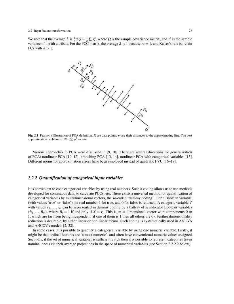
2.2 Input feature transformation 27
We note that the average λ is 1n trQ = 1
n ∑i s2i , where Q is the sample covariance matrix, and s2
i is the samplevariance of the ith attribute. For the PCC matrix, the average λ is 1 because rii = 1, and Kaiser’s rule is: retainPCs with λ > 1.
Fig. 2.1 Pearson’s illustration of PCA definition. Pi are data points, pi are their distances to the approximating line. The bestapproximation problem is UV= ∑i p2
i → min
Various approaches to PCA were discussed in [9, 10]. There are several directions for generalisationof PCA: nonlinear PCA [10–12], branching PCA [13, 14], nonlinear PCA with categorical variables [15].Different norms for approximation errors have been employed instead of quadratic FVU [16–19].
2.2.2 Quantification of categorical input variables
It is convenient to code categorical variables by using real numbers. Such a coding allows us to use methodsdeveloped for continuous data, to calculate PCCs, etc. There exists a universal method for quantification ofcategorical variables by multidimensional vectors, the so-called ‘dummy coding’ . For a Boolean variable,(with values ‘true’ or ‘false’) the real number 1 for true, and 0 for false, is returned. A categoric variable Vwith values v1, . . . ,vm can be represented in dummy coding by a battery of m indicator Boolean variables(B1, . . . ,Bm), where Bi = 1 if and only if X = vi. This is an m-dimensional vector with components 0 or1, which are far from being independent (if one of them is 1 then all others are 0). Further dimensionalityreduction is desirable, by either linear or non-linear means. Such coding is systematically used in ANOVAand ANCOVA models [2, 32].
In some cases, it is possible to quantify a categorical variable by using one numeric variable. Firstly, itmight be that ordinal features are ‘almost numeric’, and often have conventional numeric values assigned.Secondly, if the set of numerical variables is sufficiently rich then it is possible to represent categories (evennominal ones) via their average projections in the space of numerical variables (see Section 2.2.2.2 below).

28 2 Methods of Data Analysis
2.2.2.1 Ordinal feature quantification
Values of many categorical attributes are ordered linearly, by their nature: severity of a disease, qualityof a product, level of education, etc. For these attributes, we can assume that their values are obtained bybinning of a ‘latent’ numeric variable with a nice probability distribution. Usually, for this role of hypotheticallatent variable, the standard normal distribution is selected with zero mean and unit variance. Other ‘nice’distributions might be selected for quantification, for example, the uniform distribution on [0,1]. The normaldistribution has density f and cumulative distribution function CDF) φ :
f (x) =1√2π
e−x22 ; φ(x) =
∫ x
−∞
f (x)dx.
Let V be a categoric ordinal variable with linearly ordered values v1 < v2 . . . < vm. Assume that there areni cases of category vi in the sample, and the corresponding frequency is pi = ni/N (i = 1, . . . ,m). To quantifyV , it is necessary to assign an interval [ti−1, ti] to each category vi (−∞ = t0 < t1 < .. . < tm = ∞). A thresholdti separates vi from vi+1 (i = 1, . . . ,m−1). A simple calculation gives (see Fig. 2.2)
ti = φ−1
(i
∑j=1
p j
), (2.7)
where φ−1 is the inverse function of φ .
Fig. 2.2 Quantification of an ordinal feature. Three thresholds, t1, t2, and t3 are found for three categories with normalisedfrequencies p1, p2, and p3
After the thresholds ti are found, the numerical value should be selected for each category vi from theinterval [ti−1, ti]. A popular simple estimate is given by the value xi with average probability:

2.2 Input feature transformation 29
xi = φ−1
(i−1
∑j=1
p j +pi
2
). (2.8)
This value is the numeric substitution for the ordinal categoric value vi. This simple quantification methodallows a number of improvements, for instance, the values xi can be selected by the implicit maximumlikelihood method. The univariate determination of thresholds (2.7) can be generalised to the multivariateselection of the thresholds under the assumption that the multidimensional latent variables are normallydistributed. These methods are part of a set of widely used techniques for dealing with latent continuousvariables, traditionally called ‘polychoric correlation’ [25, 26].
The matrix of polychoric coefficients can be used further to calculate PCs, etc. The technique of polychoriccorrelation is based on the assumption that values of ordinal features result from the discretization ofcontinuous random values with fixed thresholds. A clear description of polychoric correlation coefficients,including methods for their estimation is given in [27, 28]. The drawback with the multivariate selection of thethresholds is in its dependence on pairs of correlated ordinal variables. If we have to analyse several dozensof such variables then a univariate choice similar to (2.7) may be preferable. A critical inquiry into polychoricand canonical correlation was published in [29]. In our work, we have used the univariate choice of thresholds(2.7) and simple average probability values (2.7) for quantification of ordinal variables. Following this, wehave applied classical methods, and also machine learning algorithms, for data analysis.
We should ask the question: are FFM, Imp, and SS scores numerical or ordinal variables? Traditionally,these scores are thought of as numerical but it is clear that this should be the case, especially if they wereobtained by short questionnaires and take a small number of values. We have taken an intermediate approach:in the analysis of average personality profiles in groups of drug users and non-users, we have handled thescores traditionally, as numeric variables, have evaluated p-values using the standard tests, calculated thePCCs with estimation of their p-values and presented the results in Tables A.1, A.2, A.3, A.4. For applicationof machine learning algorithms, we used the aforementioned procedure of quantification of ordinal features indata preprocessing, including scores, and also of the nominal features using dummy coding or CatPCA fromSubsection 2.2.2.2. The raw database is published online in [30] and the database with quantified categoricalvariables is published online in [31].
2.2.2.2 Nominal feature quantification
We cannot use the techniques described above to quantify nominal features such as gender, country of location,and ethnicity, because the categories of these features are unordered. To quantify nominal features we haveused two methods and compare the results: universal dummy coding which tremendously increases dimensionof data, and nonlinear Categorical Principal Component Analysis (CatPCA) [15].
CatPCA can be applied if there exists a rich family of numerical inputs. This method combines classicalPCA with the idea of representation of the categories of a nominal feature by the centroids of examplesfrom these categories in the space of numerical features. CatPCA assumes that the latent variable behind thenominal feature is correlated with the numerical input variables.
This procedure includes four steps (Algorithm 1).The process of nominal feature quantification for the feature ‘country’ is depicted in Fig 2.3. In this figure,
the points corresponding to the UK category are located very far from all other points.As an alternative variant of nominal feature quantification we have used dummy coding of nominal
variables: ‘country’ is transformed into seven binary features with values 1 (if ‘true’) or 0 (if ‘false’): UK,Canada, USA, Other (country), Australia, Republic of Ireland and New Zealand; Ethnicity is transformed

30 2 Methods of Data Analysis
Algorithm 1 Nominal feature quantification1: Exclude nominal features from the set of input features and calculate the PCs in the space of the numeric input features
which have been retained. To select informative PCs we use Kaiser’s rule [21, 22].2: Calculate the projection Ci of the centroid of data points from each category vi on the selected PCs.3: Consider these projections of centroids as a new dataset. Calculate the first PC of them, w.4: The numerical value for each category is the projection of its centroid on this component: vi takes the numerical value of the
inner product (w,Ci).
Fig. 2.3 Quantification of the nominal feature ‘Country’. Centroids of groups from different countries projected on the plane ofthe first two PCs of numerical input data. The line corresponds to the first PC of the set of centroids. It is worth mentioning thatthis line is originally situated in the 9-dimensional space of the selected PCs of the numeric variables. In that 9-dimensionalspace, the projections of the centroids on this line are orthogonal but this orthogonality may be lost in the two-dimensionalprojection.
into seven binary features: Mixed-White/Asian, White, Other (ethnicity), Mixed-White/Black, Asian, Blackand Mixed-Black/Asian.
2.2.3 Input feature ranking
In this study, we have used three different techniques for input feature ranking. The first technique wasprincipal variables [33]. The idea is very simple. For each attribute xi calculate the linear regression line (2.2)for predicting all other attributes. Evaluate UV, that is the sum of square errors of these predictions (for alldata points and all attributes). Select the attribute which gives the smallest FVU. This is the first principalvariable. Subtract the values predicted using the first principal variable from the data table. The new datasethas one feature less (the values of the first principal variable become zero). Iterate the above approach. We cancalculate the fraction of variance explained by kth principal variable, and the cumulative fraction of varianceexplained by the first k principal variables.
The second technique used was double Kaiser’s selection. Calculate PCs and select informative PCs, w j,by Kaiser’s rule [21, 22]. Next apply the same idea to attribute selection. PCs are normalized vectors so thatthe average of the square of their coordinates is 1/n. For each attribute find the maximal absolute value ofthe corresponding coordinates in the informative PCs: γi = max j |w ji|. The ith attribute is called trivial ifγi ≤ 1/
√n. If there are trivial attributes then the most trivial attribute is the attribute with minimal γi. We

2.3 Classification and risk evaluation 31
removed the most trivial attribute and repeated the procedure. This procedure stops if there are no trivialattributes. This algorithm ranks attributes from the most trivial to the best.
The third technique utilised was sparse PCA [34]. In this study, we employed the simplest thresholdingsparse PCA. This method returns us a list of trivial (non-important) coordinates and the sparse PCs in thespace of important coordinates. The formal description is given in Algorithm 2.
Algorithm 2 Search of sparse PC1: Set the number of attributes, n, the sample variance of the dataset, s2, and Kaiser’s threshold for the variance explained by a
component, h = s2/n.2: Search for the usual first PC with the maximal variance λ explained by this PC. (The iterative algorithm gives the PCs in
descending order of λ .)3: if λ < h then4: All the informative PCs have been found. Remove the last PC and go to Step 10.5: Find the PC coordinate with the minimal absolute value, |wmin|.6: if |wmin|> 1/
√n then
7: Go to Step 9. (All the attributes are non-trivial in this PC.)8: Set the value of the coordinate with minimal size, found at Step 5, to zero. Calculate the first PC in the reduced space of
coordinates. Go to Step 5.9: Subtract the projection onto the PC from the above PC reduction loop from the data (the dataset is redefined), and go to Step
2.10: Search the attributes, which have zero coefficients in each of the PCs found by the previous selection process. These
attributes are trivial.11: if there are trivial attributes then12: Remove trivial attributes from the set of attributes and go to Step 1. (n and s2 should be redefined.)13: else14: Stop
2.3 Classification and risk evaluation
The main classification problem studied in this book is user/non-user classification for various substancesand recency of use. The inputs include age, gender, education, N, E, O, A, C, Imp., and SS quantified, by themethods described in Sec. 2.2.2.
Several families of classification methods are applied to the solution of this problem. Most of the methodsare supplemented by risk evaluation tools.
2.3.1 Single attribute predictors
Solutions of a classification problem on the basis of one attribute are very attractive. It is nice to have onemeasurement and a red threshold line: one class is situated below this line, another class is above. Of course,such a simple rule is rarely reliable. Nevertheless, it is always a good idea to start from one-attribute classifiersand to evaluate their capabilities. It will give use a good ‘bottom line’ for evaluation of more sophisticatedclassifiers.
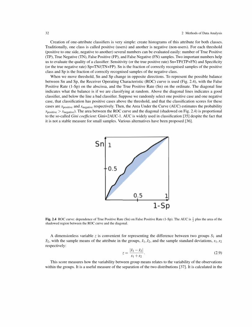
32 2 Methods of Data Analysis
Creation of one-attribute classifiers is very simple: create histograms of this attribute for both classes.Traditionally, one class is called positive (users) and another is negative (non-users). For each threshold(positive to one side, negative to another) several numbers can be evaluated easily: number of True Positive(TP), True Negative (TN), False Positive (FP), and False Negative (FN) samples. Two important numbers helpus to evaluate the quality of a classifier: Sensitivity (or the true positive rate) Sn=TP/(TP+FN) and Specificity(or the true negative rate) Sp=TN/(TN+FP). Sn is the fraction of correctly recognised samples of the positiveclass and Sp is the fraction of correctly recognised samples of the negative class.
When we move threshold, Sn and Sp change in opposite directions. To represent the possible balancebetween Sn and Sp, the Receiver Operating Characteristic (ROC) curve is used (Fig. 2.4), with the FalsePositive Rate (1-Sp) on the abscissa, and the True Positive Rate (Sn) on the ordinate. The diagonal lineindicates what the balance is if we are classifying at random. Above the diagonal lines indicates a goodclassifier, and below the line a bad classifier. Suppose we randomly select one positive case and one negativecase, that classification has positive cases above the threshold, and that the classification scores for thesecases are xpositive and xnegative respectively. Then, the Area Under the Curve (AUC) estimates the probabilityxpositive > xnegative). The area between the ROC curve and the diagonal (shadowed on Fig. 2.4) is proportionalto the so-called Gini coefficient: Gini=2AUC-1. AUC is widely used in classification [35] despite the fact thatit is not a stable measure for small samples. Various alternatives have been proposed [36].
Fig. 2.4 ROC curve: dependence of True Positive Rate (Sn) on False Positive Rate (1-Sp). The AUC is 12 plus the area of the
shadowed region between the ROC curve and the diagonal.
A dimensionless variable z is convenient for representing the difference between two groups S1 andS2, with the sample means of the attribute in the groups, x1, x2, and the sample standard deviations, s1,s2respectively:
z =|x1− x2|s1 + s2
. (2.9)
This score measures how the variability between group means relates to the variability of the observationswithin the groups. It is a useful measure of the separation of the two distributions [37]. It is calculated in the

2.3 Classification and risk evaluation 33
tables in Chapter 3 for each of seven psychological attributes and for two classes, users and non-users of illicitdrugs. The higher the score is, the better users are separated from non-users by the values of the attribute.
A simple motivation for this measure is that for the normal distributions inside groups the optimallybalanced separation of groups with given z has equal specificity and sensitivity P, where P = φ(z), recallingthat φ is the cumulative distribution function of the standard normal distribution (with µ = 0, σ = 1).Tables 3.1, 3.3, 3.5, 3.7 demonstrate that P gives realistic estimate of the empirical Sn and Sp for the dataanalysed.
The score z, its reciprocal z−1, and their multidimensional generalizations [37], are also widely used incluster analysis for the construction of criteria for the validity of clusters [39].
If we are not happy with the performance of one-attribute classifiers then it can be improved using manyapproaches. Two of them are:
• Classification by combination of the existing one-attribute classifiers (with weights defined by theirindividual performance);
• Combination of attributes to form a new multi-input discriminant function.
It is crucially important to note that when we extend the space of possible classification rules, then we addnew potential for overfitting and overoptimism. Special testing and validation procedures should be employedto avoid potentially inaccurate and misleading results. (The critical review [40] is still relevant, especiallywith respect to the new fashionable multidimensional machine learning methods).
2.3.2 Criterion for selecting the best method
A number of different criteria exist for the selection of the best classifier. If the cost of different misclassifica-tions is specified then minimisation of the expected cost can be a reasonable criterion for selection. If thecosts of different misclassifications do not vary significantly then this approach leads to the minimisation ofthe number of errors. In situations with significant class imbalance this minimization can lead to paradoxicaldecisions, for example, to the selection of a trivial rule: everything is the dominating class. The class balancein the database we use is strongly biased with respect to the general population. Therefore, we decided towork with relative criteria, which provide balanced classification rules.
The criterion we used was to pick the method such that the minimum between sensitivity and specificitywas maximised: min{Sn,Sp}→max. If min{Sn,Sp} is the same for several classifiers, then we select fromthese the classifier which maximises Sn+Sp. Classifiers with Sn or Sp less than 50% were not considered.There are several approaches to test the quality of a classifier: usage of an isolated test set, n-fold crossvalidation and Leave-One-Out Cross Validation (LOOCV) [41]. LOOCV is used for all tests in this study; weexclude a sample from the classifier preparation, learn the classifier, and then test the result on the excludedexample. Specific problems with the estimation of classifier quality for techniques like decision tree andrandom forest were considered in detail by Hastie et al. [3].
2.3.3 Linear Discriminant Analysis (LDA)
The first and the most famous tool of discriminant analysis is Fisher’s linear discriminant [38], where a newattribute is constructed as a linear functional of the given attributes, with the best classification ability. It is

34 2 Methods of Data Analysis
possible to calculate the score (2.9) for values of any function. The linear function with the highest score is aversion of the Fisher’s linear discriminant.
We used Fisher’s linear discriminant for the binary version of the problem, to separate users from non-usersof each drug. We calculate the mean of the points in the ith class, xi, and empirical covariance matrix of theith class, Si, for both classes (i = 1,2). Then we calculate the discriminating direction as
ω = (S1 +S2)−1 (x1− x2) . (2.10)
Each point is projected onto the discriminating direction by calculating the dot product (ω,xi). This projectiongives a new (combined) attribute. The optimal threshold to separate two classes is calculated.
In our study we have prepared linear discriminants for all possible selections of the subset of inputattributes, and selected the best set of inputs for each classification problem.
2.3.4 Logistic Regression (LR)
In the sequel we have implemented the weighted version of logistic regression [42]. This method can be usedfor binary problems only, and is based on the following model assumption:
probability of the first classprobability of the second class
= exp(ω,x), (2.11)
where ω is the vector of regression coefficients and x is a data vector.The maximum log likelihood estimate of the regression coefficients is used. This approach assumes that
the outcomes of different observations are independent and maximises the weighted sum of logarithms oftheir probabilities. In order to prevent class imbalance difficulties, the weights of categories are defined. Themost common weight for the ith category is the inverse of the fraction of the ith category cases among allcases. Logistic regression gives only one result because there is no option to customize the method exceptby choice of the set of input features. We performed an exhaustive search for the best set of inputs for eachclassification problem.
2.3.5 k Nearest Neighbours (kNN)
The basic concept of kNN is that the class of an object is the class of the majority of its k nearest neighbours[43]. This algorithm is very sensitive to the definition of distance. There are several commonly used variants ofdistance for kNN: Euclidean distance; Minkovsky distance; and distances calculated after some transformationof the input space. In this study, we have used three distances: the Euclidean distance, the Fisher’s transformeddistance [38], and the adaptive distance [44]. Moreover, we have used a weighted voting procedure withweighting of neighbours by one of the standard kernel functions [45].
The kNN algorithm is well-known [43]. The adaptive distance transformation algorithm is describedin [44]. kNN with Fisher’s transformed distance is less well-known. The following parameters are used: k isthe number of nearest neighbours, K is the kernel function, and k f ≥ k is the number of neighbours which areused for the distance transformation. To define the risk of drug consumption we have to perform the stepsdescribed in Algorithm 3.

2.3 Classification and risk evaluation 35
Algorithm 3 kNN with Fisher’s transformed distance1: Find the k f nearest neighbours of the test point x.2: Calculate the empirical covariance matrix of k f neighbours and Fisher’s discriminant direction.3: Find the k nearest neighbours of the x using the distance along Fisher’s discriminant direction among the k f neighbours
found earlier.4: Define the maximal distance d from x to the k neighbours.5: Calculate the membership for each class C as a sum of the weights for y ∈C. The weight of y is the ratio K(‖x− y‖/d).6: The drug consumption risk is defined as the ratio of the membership of the assigned class to the sum of memberships of all
classes.
The adaptive distance version implements the same algorithm but uses another transformation in Step 2,and another distance in Step 3 [44]. The Euclidean distance version simply defines k f = k and omits Steps 2and 3 of the algorithm. We have tested various versions of the kNN models for each drug, which differ by:
• The number of nearest neighbours, which varies between 1 and 30;• The set of input features;• One of the three distances: Euclidean distance, adaptive distance, and Fisher’s distance;• The kernel function for adaptive distance transformation;• The kernel functions for voting.• The weight of class ‘users’ is varied between 0.01 and 5.0.
2.3.6 Decision Tree (DT)
The decision tree is one of the most popular methods of data analysis [46]. It was invented before the computerera for clarification of complex diagnosis and decision making situations, in the form of a tree of simplequestions and decisions. We aim to solve the classification problem (user/non-user classification). For thispurpose, we consider a decision tree as a tool for combination of various classifiers. Each elementary classifiercan be thought of as a categorical variable X (symptom) with several nominal values v1, . . . ,vk. An elementarybranching divides the dataset (the root) into two subsets (the nodes, see Fig. 2.5). Perfect branching creates0-1 frequencies, for example n11/N1 = n22/N2 = 1 and n12 = n21 = 0. Such a perfect situation (errorlessdiagnosis by one feature) is not to be expected. However, we can find the elementary classifier, which resultsin the closest to the perfect classification. Then we can then iterate, i.e., approach each node as a dataset andtry all possible elementary classifiers, etc., until we find a perfect solution, the solution cannot be improved,or the number of examples in a node becomes too small (which will lead to overfitting).
There are many methods for developing a decision tree [47–53], which differ depending on the methodfor selection of the best elementary classifier for branching (Fig. 2.5), and by the stopping criteria. We haveevaluated the best attributes for branching using one of the following ‘gain’ functions: RIG, Gini gain, andDKM gain. They are defined in a similar way below.
Consider one node (the root, Fig. 2.5) with N cases and the binary classification problem. If the attribute Xhas c possible categorical values v1, . . . ,vc then we consider branching into c nodes. We use the followingnotation: Ni is the number of cases with X = vi (i = 1, . . . ,c), ni j (i = 1, . . . ,c, j = 1,2) is a number of casesof class j with X = vi.
For a vector of normalised frequencies f = ( f1, . . . , fk) three concave (‘Base’) functions are defined:
• Entropy( f ) =−∑ki=1 fi log2 fi;

36 2 Methods of Data Analysis
Fig. 2.5 Elementary branching in a decision tree
• Gini( f ) = 1−∑ki=1 f 2
i ;• DKM( f ) = 2
√f1 f2 (for k = 2).
The corresponding gain functions for branching are defined as
Gain = Base(n1
N,
n2
N
)−
c
∑i=1
Ni
NBase
(ni1
Ni,
ni2
Ni
),
where Base( f ) is one of the functions Entropy, Gini, or DKM.All of these Gain functions qualitatively measure the same thing: how far are distributions of nodes from
the initial distribution of the root, and how close they are to the perfect situation (when each node is stronglybiased to one of the classes).
For a variety of reasons one might want to weight classes differently, for instance, to reduce the impactof classes with many outliers. We need to multiply class frequencies by weights and then to normalise bydividing by the sum of weights.
The branching with maximal Gain is considered as the best for a given criterion function.The set of elementary classifiers (attributes) may be large, and include all the one-attribute classifiers with
different thresholds, all linear discriminants, various non-linear discriminant functions, or other classifierslike kNN, etc.
The specified minimal number of instances in a tree’s leaf is used as a criterion to stop node splitting; noleaf of the tree can contain fewer than a specified number of instances.
We tested decision tree models, which differ by:
• The three split criterion (information gain, Gini gain or DKM gain);• The use of the real-valued features in the splitting criteria separately, or in linear combination by Fisher’s
discriminant;• The set of input features;• The minimal number of instances in the leaf, which varied between 3 and 30;
2.3 Classification and risk evaluation 37
• Weight of class ‘users’ that is varied.
Direct exhaustive search of the best decision tree can lead to the overfitiing and ‘overoptimism’. Specialvalidation procedures are necessary. The standard LOOCV meets well-known problems [3] because thetopology of the tree may change in this procedure. Special notions of stability and structural stability areneeded. We return to this problem in more detail, after presentation of the classification results (Section 3.10).
2.3.7 Random Forest (RF)
Random forests were proposed by Breiman [54] for building a predictor ensemble with a set of decisiontrees that grow in randomly selected subspaces of the data [59]. The random forests classification procedureconsists of a collection of tree structured classifiers h(x,Θk),k = 1, ..., where the Θk are independent identicallydistributed random vectors and each tree casts a unit vote for the most popular class at input x [54].
In a random forest, each tree is constructed using a different bootstrap sample from the original data [3]. Instandard trees, each node is split using the best split among all variables. In a random forest, each node issplit using the best among a subset of predictors randomly chosen at that node [60].
Random forests try to improve on bagging by ‘de-correlating’ the trees. Each tree has the same expectation[3]. The forest error rate depends on two things [54]. The first is the correlation between any two trees in theforest. Increasing the correlation increases the forest error rate. The second is the strength of each individualtree in the forest. A tree with a low error rate is a strong classifier. Increasing the strength of the individualtrees decreases the forest error rate. The random forest algorithm builds hundreds of decision trees andcombines them into a single model [61].
2.3.8 Gaussian Mixture (GM)
Gaussian mixture is a method of estimating probability under the assumption that each category of a targetfeature has a multivariate normal distribution [55]. In each category we should estimate the empiricalcovariance matrix and invert it. The primary probability of belonging to the ith category is:
pi(x) = p0i (2π)−
k2 |Si|−
12 exp
[−1
2(x− xi)
′S−1i (x− xi)
]where p0
i is a prior probability of the ith category, k is the dimension of the input space, xi is the meanpoint of the ith category, x is the tested point, Si is the empirical covariance matrix of the ith category and |Si|is its determinant. The final probability of belonging to the ith category is calculated as
p fi (x) = pi(x)/∑
jp j(x).
The prior probabilities are estimated as the proportion of cases in the ith category. We also used s variedmultiplier to correct priors for the binary problem.
In the study, we tested Gaussian mixture models, which differ by the set of input features and correctionsapplied to the prior probabilities.

38 2 Methods of Data Analysis
2.3.9 Probability Density Function Estimation (PDFE)
We have implemented the radial basis function method [56] for probability density function estimation [57].The number of probability densities to estimate is equal to the number of categories of the target feature. Eachprobability density function is estimated separately by using nonparametric techniques. The prior probabilitiesare estimated from the database: pi = ni/N where ni is the number of cases in category i of the target feature,and N is the total number of cases in the database.
We also use the database to define the k nearest neighbours of each data point. These k points are used toestimate the radius of the neighbourhood of each point as a maximum of the distance from the data point toeach of its k nearest neighbours. The centre of one of the kernel functions is placed at the data point [45]. Theintegral of any kernel function over the whole space is equal to one. The total probability of the ith categoryis proportional to the integral of the sum of the kernel functions, which is equal to ni. The total probabilityof each category has to be equal to the prior probability pi. Thus, the sum of the kernel functions has to bedivided by ni and multiplied by pi. This gives the probability density estimation for each category.
We have tested a number PDFE models, which differ by:
• The number of nearest neighbours (varied between 5 and 30);• The set of the input features;• The kernel function which was placed at each data point.
2.3.10 Naıve Bayes (NB)
The NB approach is based on the simple assumption: attributes are independent. Under this assumption, wecan evaluate the distribution of the separate attributes and then produce a joint distribution function just asa product of attributes’ distributions. Surprisingly, this approach performs satisfactorily in many real lifeproblems despite the obvious oversimplification. We have used the standard version of NB [58]. All attributeswhich contain ≤20 different values were interpreted as categorical and the standard contingency tableswere calculated for such attributes. The contingency tables we calculated are used to estimate conditionalprobabilities. Attributes which contain more than 20 different values were interpreted as continuous. The meanand the variance were calculated for continuous attributes instead of the contingency tables. We calculated theisolated mean and variance for each value of the output attribute. The conditional probability of a specifiedoutcome o and a specified value of the attribute x were evaluated as the value of the probability densityfunction for a normal distribution at point x with matched mean and variance, which were calculated for theoutcome o. This method has no customization options and was tested on different sets of input features. In thestudy we tested 2,048 NB models per drug.
2.4 Visualisation on the non-linear PC canvas: Elastic maps
Elastic maps [13] provide a tool for nonlinear dimensionality reduction. By construction, they are a systemof elastic springs embedded in the data space. This system approximates a low-dimensional manifold, andis a model of the principal manifold [11, 12]. The elastic coefficients of this system allow the switch fromcompletely unstructured k-means clustering (zero elasticity) to estimators approximating linear PCs (for high
2.4 Visualisation on the non-linear PC canvas: Elastic maps 39
bending and low stretching modules). With certain intermediate values of the elasticity coefficients the systemeffectively approximates non-linear principal manifolds. In this section we follow [10].
Let the data set be a set of vectors S in a finite-dimensional Euclidean space. The ‘elastic map’ is representedby a set of nodes Wj (the ’elastic net’) in the same space, but not necessarily a subset of S. Each data points ∈ S has a ‘host node’, namely the node Wj closest to s (if there are several closest nodes then one takes thenode with the smallest index). The data set is divided in to classes
K j = {s |Wj is the host of s}.
The ‘approximation energy’ D is the distortion
D =12
k
∑j=1
∑s∈K j
‖s−Wj‖2,
which is the energy of springs with unit elasticity connecting each data point with its host node.On the set of nodes an additional structure is defined. Some pairs of nodes, (Wi,Wj), are connected by
‘elastic edges’. Denote this set of pairs E. Some triplets of nodes, (Wi,Wj,Wk), form ‘bending ribs’. Denotethis set of triplets G.
The stretching energy UE and the bending energy UG are
UE =12
λ ∑(Wi,W j)∈E
‖Wi−Wj‖2, UG =12
µ ∑(Wi,W j ,Wl)∈G
‖Wi−2Wj +Wl‖2,
where λ and µ are the stretching and bending moduli respectively. The stretching energy is sometimesreferred to as the ‘membrane’ term, while the bending energy is referred to as the ‘thin plate’ term.
For example, on the 2D rectangular grid the elastic edges are just vertical and horizontal edges (pairs ofclosest vertices) and the bending ribs are the vertical or horizontal triplets of consecutive (closest) vertices.The total energy of the elastic map is thus U = D+UE +UG. The position of the nodes {Wj} is determinedby the mechanical equilibrium of the elastic map, i.e. its location is such that it minimizes the total energy U .
For a given splitting of the dataset S in to classes K j, minimization of the quadratic functional U is a linearproblem with the sparse matrix of coefficients. Therefore, similarly to PCA or k-means, a splitting method isused:
• For given {Wj} find {K j};• For given {K j} minimize U to find new {Wj};• If no change, terminate.
This expectation-maximization algorithm guarantees a local minimum of U . To improve the approximationvarious additional methods might be proposed, for example, the ”softening” strategy. This strategy starts witha rigid grid (small length, small λ and large µ) and finishes with soft grids (small λ and µ). The training goesin several epochs, each epoch with its own grid rigidness. Another adaptive strategy is the ‘growing net’: onestarts from a small number of nodes and gradually adds new nodes. Each epoch goes with its own number ofnodes.
The elastic map is a continuous manifold. It is constructed from the elastic net using some interpolationprocedure between nodes. For example, the simplest piecewise linear elastic map is build by triangulation anda piecewise linear map. Data points are projected into the closest points of the elastic map [13].
The elastic map algorithm is extremely fast in the optimisation step due to the very simple form of thesmoothness penalty. In this book we have employed the original software libraries ViDaExpert freely available
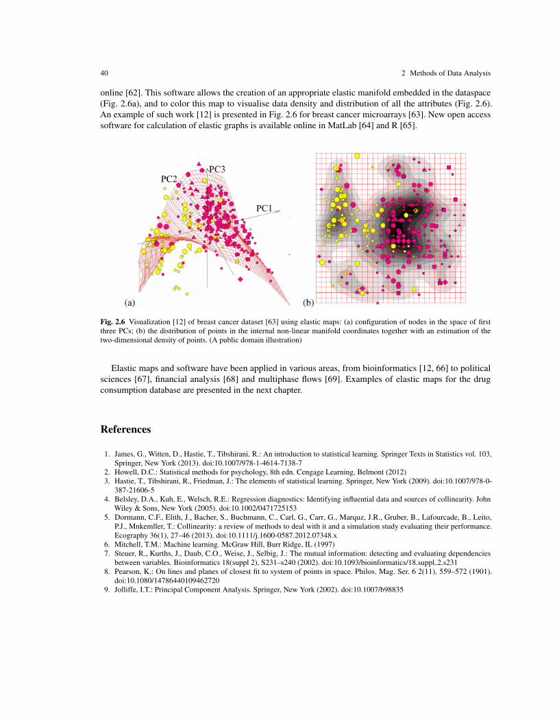
40 2 Methods of Data Analysis
online [62]. This software allows the creation of an appropriate elastic manifold embedded in the dataspace(Fig. 2.6a), and to color this map to visualise data density and distribution of all the attributes (Fig. 2.6).An example of such work [12] is presented in Fig. 2.6 for breast cancer microarrays [63]. New open accesssoftware for calculation of elastic graphs is available online in MatLab [64] and R [65].
Fig. 2.6 Visualization [12] of breast cancer dataset [63] using elastic maps: (a) configuration of nodes in the space of firstthree PCs; (b) the distribution of points in the internal non-linear manifold coordinates together with an estimation of thetwo-dimensional density of points. (A public domain illustration)
Elastic maps and software have been applied in various areas, from bioinformatics [12, 66] to politicalsciences [67], financial analysis [68] and multiphase flows [69]. Examples of elastic maps for the drugconsumption database are presented in the next chapter.
References
1. James, G., Witten, D., Hastie, T., Tibshirani, R.: An introduction to statistical learning. Springer Texts in Statistics vol. 103,Springer, New York (2013). doi:10.1007/978-1-4614-7138-7
2. Howell, D.C.: Statistical methods for psychology, 8th edn. Cengage Learning, Belmont (2012)3. Hastie, T., Tibshirani, R., Friedman, J.: The elements of statistical learning. Springer, New York (2009). doi:10.1007/978-0-
387-21606-54. Belsley, D.A., Kuh, E., Welsch, R.E.: Regression diagnostics: Identifying influential data and sources of collinearity. John
Wiley & Sons, New York (2005). doi:10.1002/04717251535. Dormann, C.F., Elith, J., Bacher, S., Buchmann, C., Carl, G., Carr, G., Marquz, J.R., Gruber, B., Lafourcade, B., Leito,
P.J., Mnkemller, T.: Collinearity: a review of methods to deal with it and a simulation study evaluating their performance.Ecography 36(1), 27–46 (2013). doi:10.1111/j.1600-0587.2012.07348.x
6. Mitchell, T.M.: Machine learning. McGraw Hill, Burr Ridge, IL (1997)7. Steuer, R., Kurths, J., Daub, C.O., Weise, J., Selbig, J.: The mutual information: detecting and evaluating dependencies
between variables. Bioinformatics 18(suppl 2), S231–s240 (2002). doi:10.1093/bioinformatics/18.suppl 2.s2318. Pearson, K.: On lines and planes of closest fit to system of points in space. Philos. Mag. Ser. 6 2(11), 559–572 (1901).
doi:10.1080/147864401094627209. Jolliffe, I.T.: Principal Component Analysis. Springer, New York (2002). doi:10.1007/b98835

References 41
10. Gorban, A.N., Zinovyev, A.Y.: Principal graphs and manifolds. In: Olivas, E.S., Guerrero, J.D.M., Sober, M.M., Benedito,J.R.M., Lopez, A.J.S. (eds.): Handbook of Research on Machine Learning Applications and Trends: Algorithms, Methods,and Techniques. pp. 28–59. IGI Global, Hershey - New York (2009). doi:10.4018/978-1-60566-766-9.ch002
11. Hastie, T., Stuetzle, W.: Principal curves. J. Am. Stat. Assoc. 84(406), 502–516 (1989). doi:10.2307/228993612. Gorban, A.N., Kegl, B., Wunsch, D.C., Zinovyev, A.Y. (eds.): Principal Manifolds for Data Visualisation and Dimension
Reduction. LNCSE, vol. 58, Springer, Berlin-Heidelberg-New York (2008). doi:10.1007/978-3-540-73750-613. Gorban, A., Zinovyev, A.: Elastic principal graphs and manifolds and their practical applications. Computing 75(4), 359–379
(2005). doi:10.1007/s00607-005-0122-614. Gorban, A.N., Zinovyev, A.Y.: Principal manifolds and graphs in practice: from molecular biology to dynamical systems.
Int. j. neural syst. 20(03), 219–232 (2010). doi:10.1142/s012906571000238315. Linting, M., van der Kooij, A.: Nonlinear principal components analysis with CATPCA: A tutorial. J. Pers. Assess. 94(1),
12–25 (2012). doi:10.1080/00223891.2011.62796516. Jolliffe, I.T., Trendafilov, N.T., Uddin, M.: A modified principal component technique based on the LASSO. J. comput.
Graph. Stat. 12(3), 531–547 (2003). doi:10.1198/106186003214817. Kwak, N.: Principal component analysis based on L1-norm maximization. IEEE trans. pattern anal. mach. intell. 30(9),
1672–1680 (2008). doi:10.1109/tpami.2008.11418. Brooks, J., Dula, J., Boone, E.: A pure L1-norm principal component analysis, Comput. Stat. Data Anal. 61, 83–98 (2013).
10.1016/j.csda.2012.11.00719. Gorban, A.N., Mirkes, E.M., Zinovyev, A.: Piece-wise quadratic approximations of arbitrary error functions for fast and
robust machine learning. Neural Netw. 84, 28–38 (2016). https://doi.org/10.1016/j.neunet.2016.08.00720. Cangelosi, R., Goriely, A.: Component retention in principal component analysis with application to cDNA microarray data,
Biol. Direct 2(1), 2 (2007). doi:10.1186/1745-6150-2-221. Guttman, L.: Some necessary conditions for common-factor analysis. Psychometrika 19(2), 149–161 (1954).
doi:10.1007/bf0228916222. Kaiser, H.F.: The application of electronic computers to factor analysis. Educ. Psychol. Meas. 20(1), 141–151 (1960).
doi:10.1177/00131644600200011623. McCrae, R.R., Costa, P.T.: A contemplated revision of the NEO five-factor inventory. Personal. Individ. Differ. 36(3),
587–596 (2004). doi:10.1016/s0191-8869(03)00118-124. Fridberg, D.J., Vollmer, J.M., O’Donnell, B.F., Skosnik, P.D.: Cannabis users differ from non-users on measures of
personality and schizotypy. Psychiatry Res. 186(1), 46–52 (2011). doi:10.1016/j.psychres.2010.07.03525. Lee, S.Y., Poon, W.Y., Bentler, P.M.: A two-stage estimation of structural equation models with continuous and polytomous
variables. Br. J. Math. Stat. Psychol. 48(2), 339–358 (1995). doi:10.1111/j.2044-8317.1995.tb01067.x26. Martinson, E.O., Hamdan, M.A.: Maximum likelihood and some other asymptotically efficient estimators of correlation in
two way contingency tables. J. Stat. Comput. Simul. 1(1), 45–54 (1971). doi:10.1080/0094965720881000327. Olsson, U.: Maximum likelihood estimation of the polychoric correlation coefficient. Psychometrika 44(4), 443–460 (1979).
doi:10.1007/bf0229620728. Drasgow, F.: Polychoric and polyserial correlations. In: Kotz, L., Johson, N.L. (eds.): Encyclopedia of statistical sciences,
vol. 7, pp. 69–74, John Wiley & Sons, New York (1988). doi:10.1002/0471667196.ess201429. Nishisato, S., Hemsworth, D.: Quantification of ordinal variables: A critical inquiry into polychoric and canonical correlation.
In: Baba, Y., Hayter, A.J., Kanefuji, K., Kuriki, S. (eds.): Recent advances in statistical research and data analysis, pp. 49–84.Springer, Tokyo (2002). doi:10.1007/978-4-431-68544-9 3
30. Fehrman, E., Egan, V.: Drug consumption, collected online March 2011 to March 2012, English-speaking countries.ICPSR36536-v1. Ann Arbor, MI: Inter-university Consortium for Political and Social Research [distributor] (2016).Deposited by Mirkes, E.M. doi:10.3886/ICPSR36536.v1
31. Fehrman, E., Egan, V., Mirkes, E.M.: Drug consumption (quantified) data set. UCI Machine Learning Repository (2016).Available https://archive.ics.uci.edu/ml/datasets/Drug+consumption+%28quantified%29. Accessed 27 Dec 2017
32. Gujarati, D.N.: Basic econometrics, 4th edn. McGraw-Hill, New York (2004)33. McCabe, G.P.: Principal variables. Technometrics 26(2), 137–144 (1984). doi:10.1080/00401706.1984.1048793934. Naikal, N., Yang, A.Y., Sastry, S.S.: Informative feature selection for object recognition via Sparse PCA. In: IEEE
International Conference on Computer Vision (ICCV) 2011, pp. 818–825, IEEE (2011). doi:10.1109/iccv.2011.612632135. Hanley, J.A., McNeil, B.J.: A method of comparing the areas under receiver operating characteristic curves derived from the
same cases. Radiology 148(3), 839–843 (1983). doi:10.1148/radiology.148.3.687870836. Hand, D.J.: Measuring classifier performance: a coherent alternative to the area under the ROC curve. Mach. learn. 77(1),
103–123 (2009). doi:10.1007/s10994-009-5119-537. Becker, P.: Recognitions of patterns. Polyteknisk, Copenhagen (1968)

42 2 Methods of Data Analysis
38. Fisher, R.A.: The use of multiple measurements in taxonomic problems. Ann. Eugen. 7(2), 179–188 (1936).doi:/10.1111/j.1469-1809.1936.tb02137.x
39. Xu, R., Wunsch, D.: Clustering. John Wiley & Sons, Hoboken, New Jersey (2008). doi:10.1002/978047038277640. Concato, J., Feinstein, A.R., Holford, T.R.: The risk of determining risk with multivariable models. Ann. intern. med.
118(3),:201–210 (1993). doi:10.7326/0003-4819-118-3-199302010-0000941. Arlot, S., Celisse, A.: A survey of cross-validation procedures for model selection. Stat. surv. 4, 40–79 (2010). doi:10.1214/09-
ss05442. Hosmer Jr, D.W., Lemeshow, S.: Applied logistic regression. John Wiley & Sons, Hoboken, NJ (2004)43. Clarkson, K.L.: Nearest-neighbor searching and metric space dimensions. In: Shakhnarovich, G., Darrell, T., Indyk, P., (eds.)
Nearest-neighbor methods for Learning and Vision: Theory and Practice, pp. 15–59. MIT Press, Cambridge, MA (2006)44. Hastie, T., Tibshirani, R.: Discriminant adaptive nearest neighbor classification. IEEE Trans. Pattern Anal. Mach. Intell.,
18(6), 607–616 (1996). doi:10.1109/34.50641145. Li, Q., Racine, J.S.: Nonparametric econometrics: theory and practice. Princeton University Press, Princeton (2007)46. Wu, X., Kumar, V., Quinlan, J.R., Ghosh, J., Yang, Q., Motoda, H., McLachlan, G.J., Ng, A., Liu, B., Philip, S.Y., Zhou,
Z.H.: Top 10 algorithms in data mining. Knowl. Inf. Syst. 14(1), 1-37 (2008). doi:10.1007/s10115-007-0114-247. Breiman, L., Friedman, J., Stone, C.J., Olshen, R.A.: Classification and regression trees. Wadsworth, Belmont, CA (1984)48. Quinlan, J.R.: Simplifying decision trees. Int. J. Man-Mach. Stud. 27(3), 221–234 (1987). doi:10.1016/s0020-7373(87)80053-
649. Rokach, L., Maimon, O.: Decision trees. In: Rokach, L., Maimon, O. (eds.): Data Mining and Knowledge Discovery
Handbook, pp. 165–192. Springer, Berlin (2010). doi:10.1007/0-387-25465-x 950. Sofeikov, K.I., Tyukin, I.Y., Gorban, A.N., Mirkes, E.M., Prokhorov, D.V., Romanenko, I.V.: Learning optimization for
decision tree classification of non-categorical data with information gain impurity criterion. In: IEEE International JointConference on Neural Network (IJCNN) 2014, pp. 3548–3555 (2014). doi:10.1109/ijcnn.2014.6889842
51. Gelfand, S.B., Ravishankar, C.S., Delp, E.J.: An iterative growing and pruning algorithm for classification tree design. IEEETrans. Pattern Anal. Mach. Intell. 13(2), 163–174 (1991). doi:10.1109/34.67645
52. Dietterich, T., Kearns, M., Mansour, Y.: Applying the weak learning framework to understand and improve C4.5. In: ICML,Proceeding of the 13th Internationsl Conference on Machine Learning, pp. 96–104. Morgan Kaufmann, San Francisco(1996)
53. Kearns, M., Mansour, Y.: On the boosting ability of top-down decision tree learning algorithms. J. Comput. Syst. Sci. 58(1),109–128 (1999). doi:10.1006/jcss.1997.1543
54. Breiman, L.: Random forests. Mach. Learn. 45(1), 5–32 (2001). doi:10.1023/a:101093340432455. Dinov, I.D.: Expectation Maximization and Mixture Modeling Tutorial. UCLA, Statistics Online Computational Resource
(2008). http://escholarship.org/uc/item/1rb70972. Accessed 27 Dec 201756. Buhmann, M.D.: Radial basis functions: theory and implementations. Cambridge University Press, Cambridge (2003).
doi:10.1017/cbo978051154324157. Scott, D.W.: Multivariate Density Estimation: Theory, Practice, and Visualization, 2nd edn. John Wiley & Sons, New York
(2015). doi:10.1002/978111857557458. Russell, S., Norvig, P.: Artificial Intelligence: a Modern Approach. Prentice Hall, Englewood Cliffs, NJ (1995).59. Biau, G.: Analysis of a random forests model. J. Mach. Learn. Res. 13, 1063–1095 (2012).60. Liaw, A., Wiener, M.R.: Classification and regression by random Forest. R news 2(3), 18–22 (2002)61. Williams, G.: Data Mining with Rattle and R: The Art of Excavating Data for Knowledge Discovery. Springer, New York –
Dordrecht – Heidelberg – London (2011). doi:10.1007/978-1-4419-9890-362. Gorban, A.N., Zinovyev, A.: Fast and user-friendly non-linear principal manifold learning by method of elastic maps. In:
IEEE International Conference on Data Science and Advanced Analytics (DSAA) 2015. doi:10.1109/dsaa.2015.734481863. Wang, Y., Klijn, J.G.M., Zhang, Y., Sieuwerts, A.M., Look, M.P., Yang, F., Talantov, D., Timmermans, M., Meijer-van Gelder,
M.E., Yu, J., Jatkoe, T., Berns, E.M.J.J., Atkins, D., Foekens, J.A.: Gene-expression profiles to predict distant metastasis oflymph-node-negative primary breast cancer. Lancet 365(9460), 671–679 (2005). doi:10.1016/s0140-6736(05)17947-1
64. Zinovyev, A., Mirkes E.M., Gorban A.N. Matlab implementation of the Elastic Principal Graphs (ElPiGraph) method (2017)https://github.com/sysbio-curie/ElPiGraph.M. Accessed 27 Dec 2017
65. Albergante L.,Zinovyev, A., Gorban A.N. An R package to construct Elastic Principal Graphs (2017)https://github.com/sysbio-curie/ElPiGraph.R. Accessed 27 Dec 2017
66. Chacon, M., Levano, M., Allende, H., Nowak, H.: Detection of gene expressions in microarrays by applying iterativelyelastic neural net. In: Adaptive and Natural Computing Algorithms. pp. 355–363. Springer, Berlin - Heidelberg (2007).doi:10.1007/978-3-540-71629-7 40
67. Zinovyev, A.: Data visualization in political and social sciences. In: Badie, B., Berg-Schlosser, D., Morlino, L. (eds.):International Encyclopedia of Political Science, SAGE (2011). doi:10.4135/9781412959636.n129
References 43
68. Resta, M.: Computational intelligence paradigms in economic and financial decision making. Springer, Cham – Heidelberg –New York – Dordrecht – London 2016. doi:10.1007/978-3-319-21440-5
69. Shaban, H., Tavoularis, S.: Identification of flow regime in vertical upward airwater pipe flow using differential pressuresignals and elastic maps. Int. J. Multiph. Flow. 61, 62–72 (2014). doi:10.1016/j.ijmultiphaseflow.2014.01.009


Chapter 3Results of data analysis
3.1 Descriptive statistics and psychological profile of illicit drug users
The data set contains seven categories of drug users: ‘Never used’, ‘Used over a decade ago’, ‘Used in lastdecade’, ‘Used in last year’, ‘Used in last month’, ‘Used in last week’, and ‘Used in last day’. A respondentselected their category for every drug from the list. We formed four classification problems based on thefollowing classes (see Section ‘Drug use’ ): the decade-, year-, month-, and week-based user/non-userseparations.
We have identified the relationship between personality profiles (NEO-FFI-R) and drug consumption forthe decade-, year-, month-, and week-based classification problems. We have evaluated the risk of drug con-sumption for each individual according to their personality profile. This evaluation was performed separatelyfor each drug for the decade-based user/non-user separation. We have also analysed the interrelations betweenthe individual drug consumption risks for different drugs. Part of these results has been presented in [1] (andin more detail in the 2015 technical report [2]). In addition, in Section 3.9 we employ the notion of correlationpleiades of drugs. We define three pleiades: heroin pleiad, ecstasy pleiad, and benzodiazepines pleiad, withrespect to the decade-, year-, month-, and week-based user/non-user separations. It is also important tounderstand how the group of users of illicit drugs differs from the group of non-users.
The descriptive statistics for seven traits (FFM, Imp, and SS) are presented in Table 3.1: means, standarddeviations, and 95% confidence intervals for means for NEO-FFI-R for the full sample and for two subsamples:non-users of illicit drugs and users of illicit drugs. We have conventionally called the following substances‘illicit’: amphetamines, amyl nitrite, benzodiazepines, cannabis, cocaine, crack, ecstasy, heroin, ketamine,legal highs, LSD, methadone, magic mushrooms (MMushrooms), and Volatile Substance Abuse (VSA).
A dimensionless variable z (see (2.9)), which measures how the variability between group relates to thevariability within the groups, is convenient for representing the difference between classes. For the normaldistributions inside groups the optimally balanced separation of groups with given z has equal specificityand sensitivity P, where P = φ(z), and φ is the cumulative distribution function for the standard normaldistribution.
This is the first result: users of illicit drugs differ from non-users across all seven scales. The 95% CIfor means in these groups do not intersect. The most significant difference was found for SS, then for O,for Imp and C, and for N. The smallest difference was found for E. Later we will demonstrate that E forusers of different drugs may deviate from E for non-users in a number of different ways. Moreover, the 95%CIs for means of all three groups, total sample, users of illicit drugs and non-users of illicit drugs do not
45

46 3 Results of data analysis
Table 3.1 Descriptive statistics: Means, 95% CIs for means, and standard deviations for the whole sample, for non-users of illicitdrugs and for users of illicit drugs (decade-based user definition). The dimensionless score z (2.9) for separation of users fromnon-users of illicit drugs is presented as well as the sensitivity and specificity P of the best separation of normal distributions withthis z. Sensitivity (Sn) and Specificity (Sp) are calculated for all one-feature classifiers. Θ is the threshold for class separation:one class is given by the inequality score≤Θ and another class by score>Θ .
Factors Total sample Non-users of illicit drugs Users of illicit drugs One feature classifierMean 95% CI SD Mean 95% CI SD Mean 95% CI SD z P(%) Θ Sn(%) Sp(%)
N 23.92 23.51, 24.33 9.14 21.00 20.29, 21.71 7.85 24.88 24.40, 25.37 9.32 0.226 59 22 60 58E 27.58 27.27, 27.88 6.77 28.52 27.99, 29.04 5.73 27.27 26.90, 27.63 7.05 0.098 54 28 51 55O 33.76 33.47, 34.06 6.58 30.22 29.67, 30.77 6.06 34.93 34.60, 35.26 6.32 0.381 65 32 63 67A 30.87 30.58, 31.16 6.44 32.87 32.35, 33.38 5.65 30.21 29.87, 30.55 6.54 0.218 59 31 61 56C 29.44 29.12, 29.75 6.97 32.89 32.39, 33.40 5.55 28.30 27.93, 28.66 7.01 0.366 64 31 65 65
Imp 3.80 3.70, 3.90 2.12 2.74 2.58, 2.90 1.74 4.15 4.04, 4.26 2.12 0.364 64 3 71 56SS 5.56 5.44, 5.68 2.70 3.77 3.56, 3.98 2.32 6.15 6.02, 6.28 2.55 0.490 69 4 63 74
intersect for N, O, A, C, Imp and SS. Table 3.1 allows us to claim that the profile of users of illicit drugs has acharacteristic form:
N ⇑,O ⇑,A ⇓,C ⇓, Imp ⇑,SS ⇑ . (3.1)
The P column in Table 3.1 gives a simple estimate of the separability of users from non-users of illicit drugsby a single trait. The best separation is given by the value of SS: estimated sensitivity and specificity are69%. According to this estimate, SS for 69% of illicit drug users is higher then SS of 69% of non-users. Ofcourse, for more precise estimation methods the numbers will differ. We might also expect that the use ofseveral attributes and more sophisticated classification approaches would give better sensitivity and specificity.Nevertheless, the P column gives us a good indication of the possible performance of classification.
Separation of classes “users of illicit drugs” and “non-users of illicit drugs” are presented in Tables 3.1–3.7,where Θ is the threshold of the separation: one class is given by the inequality score≤Θ and another classby score>Θ . This convention, where to use strong inequality, is important because the values of scores areinteger. The histogram for separation by values of SS for the decade-based definition of users is presented inFig. 3.1.
Table 3.2 gives p values, i.e. the probabilities of finding the same or larger difference between mean valuesof the traits between users of illicit drugs, non-users of illicit drugs, and the total sample. This table completelysupports the profile from (3.1).
Table 3.2 Significance of differences of means for total sample, users and nonusers of illicit drugs (p-values) for the decade-baseduser definition.
Factors Total/User Total/Non-user User/Non-userN 0.003 < 0.001 < 0.001E 0.204 0.002 < 0.001O < 0.001 < 0.001 < 0.001A 0.004 < 0.001 < 0.001C < 0.001 < 0.001 < 0.001
Imp < 0.001 < 0.001 < 0.001SS < 0.001 < 0.001 < 0.001
There are both similarity and an important qualitative difference from the ‘dark triad’ of personality,Machiavellianism, Narcissism and Psychopathy [5]. According to Table 1.2, the dark triad is associated with
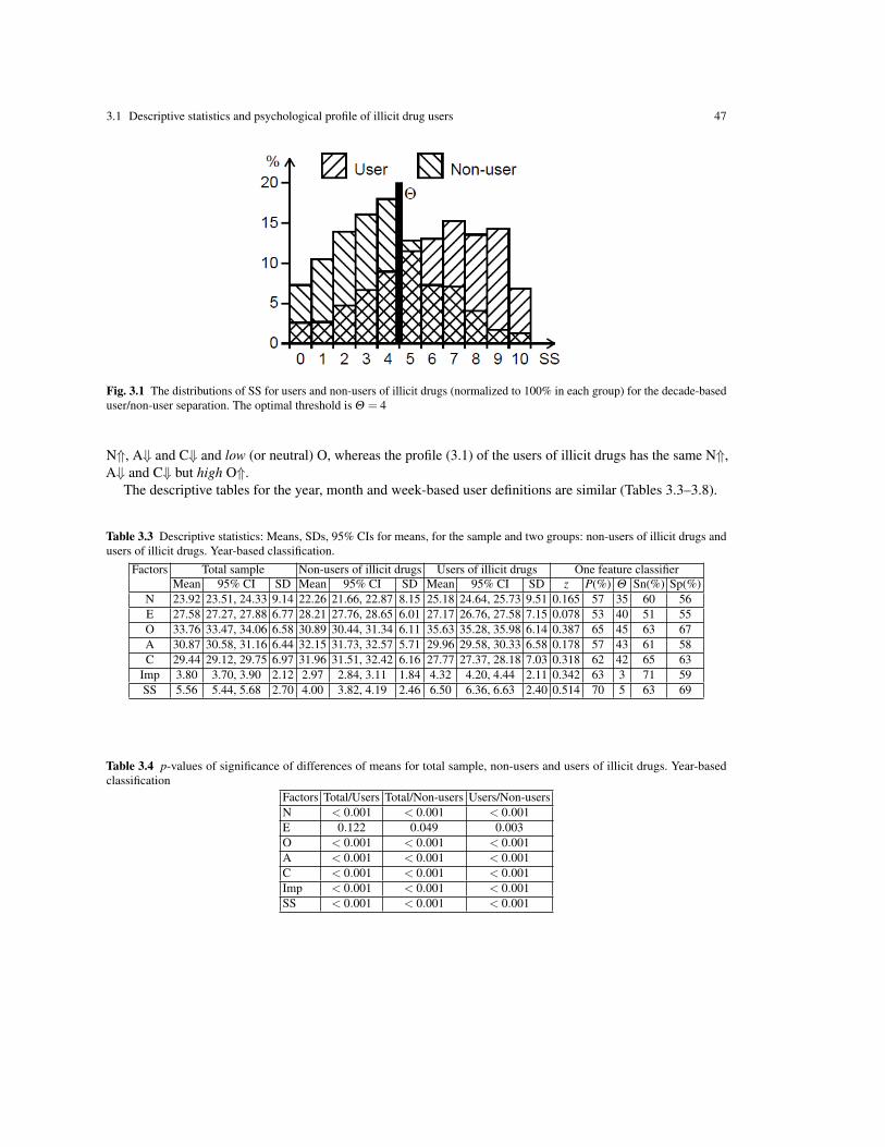
3.1 Descriptive statistics and psychological profile of illicit drug users 47
Fig. 3.1 The distributions of SS for users and non-users of illicit drugs (normalized to 100% in each group) for the decade-baseduser/non-user separation. The optimal threshold is Θ = 4
N⇑, A⇓ and C⇓ and low (or neutral) O, whereas the profile (3.1) of the users of illicit drugs has the same N⇑,A⇓ and C⇓ but high O⇑.
The descriptive tables for the year, month and week-based user definitions are similar (Tables 3.3–3.8).
Table 3.3 Descriptive statistics: Means, SDs, 95% CIs for means, for the sample and two groups: non-users of illicit drugs andusers of illicit drugs. Year-based classification.
Factors Total sample Non-users of illicit drugs Users of illicit drugs One feature classifierMean 95% CI SD Mean 95% CI SD Mean 95% CI SD z P(%) Θ Sn(%) Sp(%)
N 23.92 23.51, 24.33 9.14 22.26 21.66, 22.87 8.15 25.18 24.64, 25.73 9.51 0.165 57 35 60 56E 27.58 27.27, 27.88 6.77 28.21 27.76, 28.65 6.01 27.17 26.76, 27.58 7.15 0.078 53 40 51 55O 33.76 33.47, 34.06 6.58 30.89 30.44, 31.34 6.11 35.63 35.28, 35.98 6.14 0.387 65 45 63 67A 30.87 30.58, 31.16 6.44 32.15 31.73, 32.57 5.71 29.96 29.58, 30.33 6.58 0.178 57 43 61 58C 29.44 29.12, 29.75 6.97 31.96 31.51, 32.42 6.16 27.77 27.37, 28.18 7.03 0.318 62 42 65 63
Imp 3.80 3.70, 3.90 2.12 2.97 2.84, 3.11 1.84 4.32 4.20, 4.44 2.11 0.342 63 3 71 59SS 5.56 5.44, 5.68 2.70 4.00 3.82, 4.19 2.46 6.50 6.36, 6.63 2.40 0.514 70 5 63 69
Table 3.4 p-values of significance of differences of means for total sample, non-users and users of illicit drugs. Year-basedclassification
Factors Total/Users Total/Non-users Users/Non-usersN < 0.001 < 0.001 < 0.001E 0.122 0.049 0.003O < 0.001 < 0.001 < 0.001A < 0.001 < 0.001 < 0.001C < 0.001 < 0.001 < 0.001Imp < 0.001 < 0.001 < 0.001SS < 0.001 < 0.001 < 0.001

48 3 Results of data analysis
Table 3.5 Descriptive statistics: Means, SDs, 95% CIs for means, for the sample and two groups: non-users of illicit drugs andusers of illicit drugs. Month-based classification
Factors Total sample Non-users of illicit drugs Users of illicit drugs One feature classifierMean 95% CI SD Mean 95% CI SD Mean 95% CI SD z P(%) Θ Sn(%) Sp(%)
N 23.92 23.51, 24.33 9.14 22.60 22.06, 23.14 8.22 25.13 24.53, 25.73 9.69 0.141 56 35 56 60E 27.58 27.27, 27.88 6.77 28.27 27.89, 28.65 5.78 27.19 26.74, 27.64 7.27 0.083 53 39 56 51O 33.76 33.47, 34.06 6.58 31.01 30.60, 31.43 6.24 36.04 35.67, 36.41 6.00 0.411 66 45 63 63A 30.87 30.58, 31.16 6.44 31.82 31.43, 32.22 6.02 29.81 29.40, 30.22 6.65 0.159 56 43 56 61C 29.44 29.12, 29.75 6.97 31.78 31.38, 32.17 5.97 27.50 27.06, 27.95 7.15 0.326 63 42 61 65
Imp 3.80 3.70, 3.90 2.12 3.04 2.91, 3.16 1.92 4.43 4.30, 4.56 2.08 0.348 64 3 64 71SS 5.56 5.44, 5.68 2.70 4.15 3.99, 4.32 2.51 6.68 6.54, 6.83 2.35 0.521 70 5 67 63
Table 3.6 p-values of significance of differences of means for total sample,non-users and users of illicit drugs. Month-basedclassification
Factors Total/Users Total/Non-users Users/Non-usersN 0.001 0.002 < 0.001E 0.166 0.024 0.002O < 0.001 < 0.001 < 0.001A < 0.001 0.003 < 0.001C < 0.001 < 0.001 < 0.001Imp < 0.001 < 0.001 < 0.001SS < 0.001 < 0.001 < 0.001
Table 3.7 Descriptive statistics: Means, SDs, 95% CIs for means, for the sample and two groups: non-users of illicit drugs andusers of illicit drugs. Week-based classification
Factors Total sample Non-users of illicit drugs Users of illicit drugs One feature classifierMean 95% CI SD Mean 95% CI SD Mean 95% CI SD z P(%) Θ Sn(%) Sp(%)
N 23.92 23.51, 24.33 9.14 22.79 22.27, 23.31 8.47 25.21 24.56, 25.86 9.72 0.133 55 35 55 60E 27.58 27.27, 27.88 6.77 28.34 27.97, 28.71 5.96 27.09 26.60, 27.58 7.33 0.094 54 39 56 51O 33.76 33.47, 34.06 6.58 31.18 30.78, 31.57 6.37 36.17 35.77, 36.57 5.99 0.404 66 46 66 63A 30.87 30.58, 31.16 6.44 31.63 31.25, 32.01 6.18 29.80 29.35, 30.24 6.67 0.143 56 42 60 61C 29.44 29.12, 29.75 6.97 31.57 31.20, 31.95 6.10 27.41 26.94, 27.89 7.10 0.315 62 41 64 65
Imp 3.80 3.70, 3.90 2.12 3.10 2.99, 3.22 1.94 4.45 4.31, 4.59 2.08 0.335 63 3 61 71SS 5.56 5.44, 5.68 2.70 4.27 4.12, 4.43 2.52 6.73 6.58, 6.89 2.35 0.505 69 5 62 63
Table 3.8 P-values of significance of differences of means for total sample, non-users and users of illicit drugs. Week-basedclassification
Factors Total/Users Total/Non-users Users/Non-usersN 0.001 0.011 < 0.001E 0.100 0.016 0.001O < 0.001 < 0.001 < 0.001A < 0.001 0.018 < 0.001C < 0.001 < 0.001 < 0.001Imp < 0.001 < 0.001 < 0.001SS < 0.001 < 0.001 < 0.001
Pearson’s correlation coefficient (PCC or r) is employed as a measure of the strength of a linear associationbetween two factors. PCC for all pairs of factors are presented in Table 3.9. Two pairs of factors do not have

3.2 Distribution of number of drugs used 49
significant correlation: (1) N and O (r=0.017, p=0.471); (2) A and O (r=0.033, p=0.155). However, all otherpairs of personality factors are significantly correlated in the sample (compare to Table 1.3).
Table 3.9 PCC for NEO-FFI-R for raw dataFactors N E O A C
N -0.432* 0.017 -0.215* -0.398*
E -0.432* 0.236* 0.159* 0.318*
O 0.017 0.236* 0.033 -0.060**
A -0.215* 0.159* 0.033 0.249*
C -0.398* 0.318* -0.060** 0.249*
*p < 0.001; **p < 0.01.
Strictly speaking, the scores should be considered as ordinal features. Therefore, the polychoric correlationcoefficients (PoCC) should be used. Table 3.10 presents values of PoCCs between all of the psychologicaltraits we measured (compare to Tables 1.3 and 3.9). The corresponding p-values are presented in Table 3.1.
Table 3.10 Polychoric correlation coefficients (PoCC) of measured psychological traits (n=1,885).
N E O A C Imp SSN −0.431* 0.010 −0.217* −0.391* 0.174* 0.080**E −0.431* 0.245* 0.157* 0.308* 0.114* 0.210*O 0.010 0.245* 0.039 −0.057*** 0.278* 0.422*A −0.217* 0.157* 0.039 0.247* −0.230* −0.208*C −0.391* 0.308* −0.057*** 0.247* −0.335* −0.229*
Imp 0.174* 0.114* 0.278* −0.230* −0.335* 0.623*SS 0.080** 0.210* 0.422* −0.208* −0.229* 0.623*
*p < 0.0001, **p < 0.001, ***p < 0.02.
3.2 Distribution of number of drugs used
The diagrams in Fig. 3.2 show the graph of the number of users versus the number of illicit drugs used for thedecade-based (a) and month-based (b) user/non-user separations. In Fig. 3.2 a we can see that the distributionof the number of users is bimodal with maxima at zero and seven drugs used. In Fig. 3.2 b the distribution ofthe number of users of various numbers of illegal drugs during the last months looks like the exponentialdistribution.
The distributions of the number of users for each drug are presented in Fig. 3.3 and Fig. 3.4. Most of thedistributions have an exponential-like shape, but several have bimodal distributions. The distributions of thenumber of users for the three legal drugs have maximum at ‘Used in last day’ or ‘Used in last week’ (seeFig. 3.3 a, e, and g). The distribution of the number of nicotine users (smokers) has three maxima: ‘Usedin last day’ for smokers, ‘Used in last decade’ for smokers who have quit smoking, and ‘Never used’ (seeFig. 3.4 g). All distributions for illegal drug users have maximum in the category ‘Never used’. However, thedistribution of cannabis users has two maxima. The main maximum is in the category ‘Used in last day’, andthe second is in the category ‘Never used’ (see Fig. 3.3f).

50 3 Results of data analysis
Fig. 3.2 The histograms of the number of users of illicit drugs (the number of users versus the number of illicit drugs used): (a)for the decade-based user/non-user separation, and (b) for the month-based user/non-user separation
3.3 Sample mean and population norm
It may seem to be a good idea to use the T-scores with respect to the population norm. Caution is neededhowever, since the mean values may depend on age and social group, so that the notion of ‘population norm’is a complex hierarchical construct rather than a simple set of means.
Following [3] we include data about two groups. The first consists of high school students (n=1959) [6].The age range is from 14 to 18 (M=16.5, S.D.=1.0 years); approximately two-thirds were girls. In Table 3.11,we denote this group with the abbreviation HS.
The second sample consists of adults from the Baltimore Longitudinal Study of Aging (BLSA) [7]. BLSAparticipants are generally healthy and well-educated men and women who have volunteered to return to theGerontology Research Center for periodic medical and psychosocial testing. The data was collected between1991 and 2002, n=1,492 (695 men and 797 women) aged 19–93 (M=56.2, S.D.=17.0 years); 65.1% of thesample was White, 27.6% Black, and 7.3% Other Race. In Table 3.11 we refer to this group as BLSA.
The third sample includes 1,025 participants (802 males and 221 females; two individuals did not provideinformation on their gender) and combines data from several studies published between 1996–2000 [8]. Thiscohort had a good range of skills, mental ability, and psychopathology, and aimed to be a representativecross-section of British society. In Table 3.11, we use Brit to label this group.
For HS and BLSA data both NEO-FFI and NEO-FFI-R profiles are available. For Brit only the NEO-FFIscores are available. For ease of comparison we include the Five Factor scores for our sample and for thesubsample of illicit drug users (Table 3.1) in Table 3.11.
The means of the NEO-FFI-R T-scores based on normative data are depicted in Fig. 3.5. For this example,the ‘norm’ is taken from the BLSA group (NEO-FFI). It is obvious from this figure that Samp is significantlybiased when compared to the population (represented by the BLSA group). Such a bias is usual for clinicalcohorts, for example, the ‘problematic’ or ‘pathological’ groups [9], and the drug users [10, 11]. For the groupof non-users of illicit drugs the bias is much smaller.
It is important to observe that the mean values of scores for four factors in our sample, N, E, A, and C, arebetween the mean scores for BLSA and HS. The mean O score in our sample is significantly higher.
The special role of “Openness to Experience” (O) for drug consumption has been observed by manyresearchers. For example, in the paper “Undergraduate marijuana and drug use as related to openness toexperience” [12] we read: “Marijuana use, in the present sample of college students, was associated withpersonality characteristics which many would tend to value (e.g., creativity). Open mindedness or ‘opennessto experience’ may account for our findings. People who are open to new experience become creative, trymarijuana, and, in general, experience more than people who have a less open life style. This accounts for
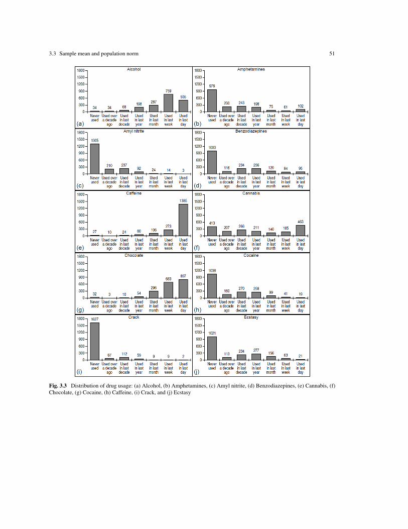
3.3 Sample mean and population norm 51
Fig. 3.3 Distribution of drug usage: (a) Alcohol, (b) Amphetamines, (c) Amyl nitrite, (d) Benzodiazepines, (e) Cannabis, (f)Chocolate, (g) Cocaine, (h) Caffeine, (i) Crack, and (j) Ecstasy

52 3 Results of data analysis
Fig. 3.4 Distribution of drug usage: (a) Heroin, (b) Ketamine, (c) Legal highs, (d) LSD, (e) Methadone, (f) MMushrooms, (g)Nicotine, and (h) VSA
our finding that the more a person uses marijuana, the more likely they are to try one or more other drugs.”Non-users were characterised as “the typical non-creative, high authoritarian individuals.”
The high variability of means in the ‘normal’ groups has encouraged us to analyse the T-scores withrespect to the sample mean and to study the differences between users and non-users rather than deviationfrom the norm. This analysis is presented in the next two sections.

3.4 Deviation of the groups of drug users from the sample mean 53
Table 3.11 Mean values of Five Factors for the three ‘normal’ samples and for our data.‘ N-u, Illicit’ stands for non-users ofillicit drugs with the decade-based definition of users (they either never used illicit drugs or used them more than a decade ago),Samp stands for the total sample, ‘U, Illicit’ stands for users of illicit drugs for the decade-based definition of users; comparewith Table 3.1
N E O A CGroup Version Mean SD Mean SD Mean SD Mean SD Mean SD
BLSA NEO-FFI 15.77 7.47 28.50 6.26 29.32 6.11 33.39 4.98 33.48 6.36NEO-FFI-R 16.83 7.36 29.29 6.46 31.29 6.12 32.41 5.42 33.26 6.30
HS NEO-FFI 24.65 8.07 30.58 6.67 28.40 6.57 28.31 6.34 27.45 7.30NEO-FFI-R 25.08 7.95 31.80 6.94 31.18 6.96 28.09 6.93 27.00 7.40
Brit NEO-FFI 19.5 8.6 27.1 5.9 26.5 6.5 29.7 5.9 32.1 6.6N-u, Illicit NEO-FFI-R 21.00 7.85 28.52 5.73 30.22 6.06 32.87 5.65 32.89 5.55Samp NEO-FFI-R 23.92 9.14 27.58 6.77 33.76 6.58 30.87 6.44 29.44 6.97U, Illicit NEO-FFI-R 24.88 9.32 27.27 7.05 34.93 6.32 30.21 6.54 28.30 7.01
Fig. 3.5 Mean T-score NEO-FFI-R for the total sample and for non-users of illicit drugs with respect to the BLSA mean as anorm
3.4 Deviation of the groups of drug users from the sample mean
Tables A.1 and A.2 demonstrate the mean T-scoresample of five NEO-FFI-R factors, supplemented by Impand SSs for users and non-users, for each drug with respect to the decade-, year-, month-, and week-basedclassification problems respectively (see Appendix A). Significant differences in personality factor scoresare observed between these groups. The hypothesis about the universal relationship between personalityprofile and the risk of drug consumption can generally be described as in (3.1): an increase in scores of N, O,Imp, and SS suggest an increase in the risk of use, whereas an increase in the scores of A and C results in adecrease in the risk of use. Thus for each drug, drug users scored higher on N and O, and lower on A and C,when compared to non-users of drugs. The influence of the score of E is drug specific (non-universal).
We now analyse the sign of T-scoresample for various drugs and the definitions of users (decade-, year-,month- and week-based). We used a + sign for moderately high and high T-scoresample (T-scoresample > 55,and a – sign for moderately low and low T-scoresample (T-scoresample < 45, and 0 for a score close to the meanvalue 55≥T-scoresample ≥ 45. These signs reflect the distance from the group of users to the sample mean.
In the next section we analyse significance of deviations. There is a standard and well-known problemwith reporting of the values and significance of deviations: ‘significant’ does not mean ‘large’ and, conversely,apparently large deviations could be insignificant. Everything is defined by interplay between the numberof elements in classes and the deviation value. Practically, significant but small deviations may be unstable:after small change of conditions they may even change their sign. We consider the variability of the ‘normal’

54 3 Results of data analysis
scores in Section 3.3. Insignificant but apparently large deviation may become significant for larger samplesor may vanish. Therefore, it is necessary to answer two questions: how large is the deviation (this section)and how significant is it (next section)?
For a significant deviation of users from non-users we use the signs ⇑ and ⇓.The inclusion of moderate subcategories of T-scoresample as suggested above enables us to separate the
drugs into five groups for the decade-based user/non-user separation. These are presented in Table 3.12. Eachgroup can be coded using the (N, E, O, A, C, Imp, SS) profile:
• The group with the profile (0,0,0,0,0,0,0) includes the users of three legal drugs: alcohol, chocolate andcaffeine;
• The group of drugs with the profile (0,0,+,−,−,+,+) includes the users of amyl nitrite, LSD, and magicmushrooms;
• Nicotine users form their own group with the profile (0,0,+,0,−,+,+);• The largest group of drugs with the profile (+,0,+,−,−,+,+) includes the users of amphetamines,
benzodiazepines, cannabis, cocaine, ecstasy, ketamine, and legal highs;• Finally, the group with the profile (+,−,+,−,−,+,+) includes the users of crack, heroin, VSA and
methadone.
Table 3.12 Deviation of T-scoresample from the sample mean for various groups of users for the decade-based user/non-userseparation
Drug N E O A C Imp SSAlcohol, Chocolate, Caffeine 0 0 0 0 0 0 0Amyl nitrite, LSD, and MMushrooms 0 0 + − − + +Nicotine 0 0 + 0 − + +Amphetamines, Benzodiazepines, Cannabis,Cocaine, Ecstasy, Ketamine, and Legal highs + 0 + − − + +
Crack, Heroin, VSA, and Methadone + − + − − + +Ecstasy pleiad 0 0 + − − + +Heroin pleiad, Benzodiazepines pleiad + 0 + − − + +Illicit drugs + 0 + − − + +
For the year-based user/non-user classification, drugs are separated into eight groups as presented inTable 3.13. Each group can be coded using the (N, E, O, A, C, Imp, SS) profile:
• The group with the profile (0,0,0,0,0,0,0) includes the users of three legal drugs alcohol, chocolate andcaffeine;
• The group of drugs with the profile (0,0,+,−,−,+,+) contains just the users of magic mushrooms;• The LSD users also form their own group with the profile (0,0,+,0,−,+,+);• The group with the profile (+,0,+,−,−,+,+) includes the users of amphetamines, amyl nitrite, cannabis,
cocaine, crack, legal highs and VSA;• The group of drugs with the profile (+,−,+,−,−) includes the users of benzodiazepines, heroin, and
methadone;• The ecstasy users form their own group with the profile (0,+,+,−,−,+,+);• The ketamine users form their own group with the profile (+,+,+,−,−,+,+);• The nicotine users form their own group with the profile (+,0,+,0,−,+,+).

3.4 Deviation of the groups of drug users from the sample mean 55
Similarly, the deviations of T-scoresample from the sample mean for the month-based user/non-userclassification and for the week-based user/non-user classification are described in Table 3.14 and Table 3.15respectively.
Table 3.13 Deviation of T-scoresample from the sample mean for various groups of users for the year-based user/non-userseparation
Drug N E O A C Imp SSAlcohol, Chocolate, Caffeine 0 0 0 0 0 0 0MMushrooms 0 0 + − − + +LSD 0 0 + 0 − + +Amphetamines, Amyl nitrite, Cannabis,Cocaine, Crack, Legal highs, and VSA + 0 + − − + +
Benzodiazepines, Heroin, and Methadone + − + − − + +Ecstasy 0 + + − − + +Ketamine + + + − − + +Nicotine + 0 + 0 − + +Heroin pleiad, Ecstasy pleiad, Benzodiazepines pleiad + 0 + − − + +Illicit drugs + 0 + − − + +
Table 3.14 Deviation of T-scoresample from the sample mean for various groups of users for the month-based user/non-userseparation
Drug N E O A C Imp SSAlcohol, Chocolate, Caffeine 0 0 0 0 0 0 0Cannabis and MMushrooms 0 0 + − − + +Nicotine + 0 + 0 − + +Amphetamines, Ketamine, and Legal highs + 0 + − − + +Benzodiazepines, Heroin, and Methadone + − + − − + +Ecstasy and LSD 0 + + − − + +Cocaine and VSA + + + − − + +Amyl nitrite 0 0 0 − − + +Crack + − 0 − − + +Ecstasy pleiad 0 0 + − − + +Heroin pleiad, Benzodiazepines pleiad + − + − − + +Illicit drugs + 0 + − − + +
The personality profiles are strongly associated with membership of groups of the users and non-usersof the 18 drugs. We found that the N and O score of drug users of all 18 drugs are moderately high (+) orneutral (0), and that the A and C scores of drug users are moderately low (−) or neutral (0). Detailed resultscan be seen in Tables 3.13, 3.14, and 3.15.
The effect of the E score is drug specific. Drugs are divided into three groups with respect to the E score ofusers (in the year-, month-, and week-based classification problems; see Tables 3.12, 3.13, 3.14 and 3.15. Forexample, for the week-based user/non-user separation the E score is:
• Moderately low (−) in groups of users of amphetamines, amyl nitrite, benzodiazepines, heroin, ketamine,legal highs, methadone, and crack;
• Moderately high (+) in groups of users of cocaine, ecstasy, LSD, magic mushrooms, and VSA;

56 3 Results of data analysis
Table 3.15 Deviation of T-scoresample from the sample mean for various groups of users for the week-based user/non-userseparation
Drug N E O A C Imp SSAlcohol, Chocolate, Caffeine 0 0 0 0 0 0 0Cannabis 0 0 + − − + +LSD and MMushrooms 0 + + 0 − + +Ketamine 0 − + − − + +Amphetamines, Benzodiazepines,Heroin, Legal highs, and Methadone + − + − − + +
Ecstasy 0 + + − − + +VSA 0 + + − 0 + +Cocaine + + + − − + +Nicotine + 0 + 0 − + +Amyl nitrite 0 − 0 − − + +Crack + − − − − + +Heroin pleiad, Benzodiazepines pleiad + − + − − + +Ecstasy pleiad 0 0 + − − + +Illicit drugs + 0 + − − + +
• Neutral (0) in groups of users of alcohol, caffeine, chocolate, cannabis, and nicotine.
3.5 Significant differences between groups of drug users and non-users
Tables 3.16, 3.17, 3.18, and 3.19 (“user minus non-user profiles”) show where there are significant differencesbetween the means of the personality traits for the groups of users and non-users for the decade-, year-,month-, and week-based classification problems respectively. Three significance level are used:
• 99% significance level (p-value is less than 0.01). Symbol ‘⇓ ’ corresponds to 99% significant differencewhere the mean in users group is less than mean in non-users group and symbol ‘⇑’ corresponds to 99%significant difference where the mean in users group is greater than the mean in non-users group.
• 98% significance level (p-value is less than 0.02). Symbol ‘↓ ’ corresponds to 98% significant differencewhere the mean in users group is less than mean in non-users group and symbol ‘↑’ corresponds to 98%significant difference where the mean in users group is greater than the mean in non-users group.
• 95% significance level (p-value is less than 0.05). Symbol ‘� ’ corresponds to 95% significant differencewhere the mean in users group is less than mean in non-users group and symbol ‘�’ corresponds to 95%significant difference where the mean in users group is greater than the mean in non-users group.
Empty cells in the tables below correspond to insignificant differences.For example for the decade-based user/non-user separation (see Table 3.16) chocolate does not have a
significant difference between users and non-users for any of the factors. Alcohol users and non-users onlyhave a 99% significant difference in the C , Imp, and SS scores, and 95% significant difference in the A score.According to Table 3.12 all these deviations are small.
LSD and magic mushrooms for the decade-based user/non-user separation (see Table 3.16) have 99%significant difference between users and non-users in the O, A, C, Imp, and SS scores and 95% significantdifference in the N score. According to Table 3.12 both for LSD and magic mushrooms the deviation in the Nscore is small and all the deviations in the O, A, C, Imp, and SS scores are not small.

3.5 Significant differences between groups of drug users and non-users 57
In Table 3.16, benzodiazepines and methadone have 99% significant differences between users andnon-users in all seven scores. For methadone, all of these differences are not small (Table 3.12) and forbenzodiazepines the difference in the E score is small inspite of having 99% significance.
The significance of the differences of the means for groups of users and non-users for the year, month,and week-based user definition is presented in Tables 3.17–3.19. We hope that the previous descriptions ofwhere the significant differences lie are enough for the reader to interpret this table. It is useful to considersignificance of differences together with their value (Tables 3.13– 3.15). Additional information about thesedifferences could be extracted from the detailed Tables A.1, A.2 in the Appendix.
Table 3.16 Significant differences of means for groups of users and non-users for the decade-based user/non-user separation.
Drug N E O A C Imp SSChocolateAlcohol � ⇓ ⇑ ⇑Amyl nitrite ⇑ ⇓ ⇓ ⇑ ⇑Caffeine � ⇑ ↓ ↑ ⇑LSD, MMushrooms � ⇑ ⇓ ⇓ ⇑ ⇑Amphetamine, Cocaine, Crack, Ecstasy, Ketamine, Legal highs, Nicotine, VSA ⇑ ⇑ ⇓ ⇓ ⇑ ⇑Cannabis, Heroin ⇑ � ⇑ ⇓ ⇓ ⇑ ⇑Benzodiazepines, Methadone ⇑ ⇓ ⇑ ⇓ ⇓ ⇑ ⇑Benzodiazepines pleiad, Heroin pleiad ⇑ ⇑ ⇓ ⇓ ⇑ ⇑Ecstasy pleiad ⇑ � ⇑ ⇓ ⇓ ⇑ ⇑Illicit drugs ⇑ ⇓ ⇑ ⇓ ⇓ ⇑ ⇑
Table 3.17 Significant differences of means for groups of users and non-users for the year-based user/non-user separation.
Drug N E O A C Imp SSChocolateAlcohol ⇑Amyl nitrite ↑ ⇓ ⇓ ⇑ ⇑LSD ⇑ � ⇓ ⇑ ⇑MMushrooms ⇑ ⇓ ⇓ ⇑ ⇑Caffeine ↑ � � ⇑ ⇑Ecstasy ⇑ ⇑ ⇓ ⇓ ⇑ ⇑Ketamine ↑ ⇑ ⇓ ⇓ ⇑ ⇑VSA ⇑ ⇑ ↓ ⇓ ⇑ ⇑Amphetamine, Cannabis, Crack, Legal highs, Nicotine ⇑ ⇑ ⇓ ⇓ ⇑ ⇑Cocaine ⇑ � ⇑ ⇓ ⇓ ⇑ ⇑Heroin ⇑ ↓ ⇑ ⇓ ⇓ ⇑ ⇑Benzodiazepines, Methadone ⇑ ⇓ ⇑ ⇓ ⇓ ⇑ ⇑Heroin pleiad ⇑ ⇑ ⇓ ⇓ ⇑ ⇑Benzodiazepines pleiad, Ecstasy pleiad ⇑ � ⇑ ⇓ ⇓ ⇑ ⇑Illicit drugs ⇑ ⇓ ⇑ ⇓ ⇓ ⇑ ⇑
Mean values of Five Factor scores for groups of drug users and non-users for the decade-based user/non-user separation are depicted in Fig. 3.6. Some similarities and differences between users of different drugs areobvious from this figure: compare, for example, profiles of ecstasy users and heroin users, which are verydifferent to profiles for nicotine and cannabis users, which are qualitatively similar (but with larger deviations

58 3 Results of data analysis
Table 3.18 Significant differences of means for groups of users and non-users for the month-based user/non-user separation.
Drug N E O A C Imp SSChocolateAmyl nitrite ↓ � ↑ ⇑LSD, MMushrooms ⇑ ⇓ ⇑ ⇑VSA ⇑ � ⇑ ⇑Ketamine ⇑ � ⇓ ⇑ ⇑Caffeine ⇑ ⇑ ⇑Alcohol ⇑ � ⇑Ecstasy ⇑ ⇑ ⇓ ⇓ ⇑ ⇑Crack ⇑ � � ↑ ⇑Amphetamine, Cannabis, Cocaine, Legal highs, Nicotine ⇑ ⇑ ⇓ ⇓ ⇑ ⇑Heroin ⇑ ↓ ⇓ ⇓ ⇑ ⇑Benzodiazepines, Methadone ⇑ ⇓ ⇑ ⇓ ⇓ ⇑ ⇑Ecstasy pleiad, Heroin pleiad ⇑ ⇑ ⇓ ⇓ ⇑ ⇑Benzodiazepines pleiad ⇑ ⇓ ⇑ ⇓ ⇓ ⇑ ⇑Illicit drugs ⇑ ⇓ ⇑ ⇓ ⇓ ⇑ ⇑
Table 3.19 Significant differences of means for groups of users and non-users for the week-based user/non-user separation.
Drug N E O A C Imp SSChocolate ↓Crack � � ⇑Amyl nitrite � � � ⇑Ketamine ↑ ↓ ↓ ↑ ⇑VSA ⇑ ⇑ ⇑LSD ⇑ ⇓ � ⇑Cannabis ⇑ ⇓ ⇓ ⇑ ⇑MMushrooms � ⇑ ⇑ ⇑Caffeine ↑ �Ecstasy ↑ ⇑ ⇓ ⇑ ⇑Alcohol ⇑ ⇑Cocaine ↑ ⇓ ⇓ ⇑ ⇑Amphetamine, Nicotine ⇑ ⇑ ⇓ ⇓ ⇑ ⇑Heroin ⇑ � ⇓ ⇓ ⇑ ⇑Methadone ⇑ ⇓ � ⇓ ⇓ ⇑ ⇑Benzodiazepines, Legal highs ⇑ ⇓ ⇑ ⇓ ⇓ ⇑ ⇑Ecstasy pleiad ⇑ ⇑ ⇓ ⇓ ⇑ ⇑Benzodiazepines pleiad, Heroin pleiad ⇑ ⇓ ⇑ ⇓ ⇓ ⇑ ⇑Illicit drugs ⇑ ⇓ ⇑ ⇓ ⇓ ⇑ ⇑
of cannabis users profiles from the sample mean). Mean values of all seven factor scores for groups of drugusers and non-users for all definitions of users are presented in Tables A.1 and A.2.
3.6 Correlation between usage of different drugs
Usage of each drug is a binary variable (users or non-users) for all versions of user definition. Tables A.3and A.4 contain PCCs, which are computed for each pair of the 153 (=18 times 17 divided by 2) potential
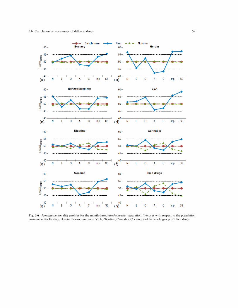
3.6 Correlation between usage of different drugs 59
Fig. 3.6 Average personality profiles for the month-based user/non-user separation. T-scores with respect to the populationnorm mean for Ecstasy, Heroin, Benzodiazepines, VSA, Nicotine, Cannabis, Cocaine, and the whole group of Illicit drugs

60 3 Results of data analysis
drug usages for the decade- and year-based user/non-user separations respectively (see Appendix A.2). Themajority of the PCCs are significant, since the sample size is 1,885.
The correlation in 124 pairs of drug usages from a totality of 153 pairs have, for the decade-basedclassification problem, p-values less than 0.01 (p-value is the probability of observing by chance the same orgreater correlation coefficient for uncorrelated variables). It is necessary to employ a multi-testing approachwhen testing 153 pairs of drug usages in order to estimate the significance of the correlation [13]. We applythe most conservative technique, the Bonferroni correction, and used the Benjamini-Hochberg (BH) step-upprocedure [13] to control the False Discovery Rate (FDR) in order to estimate the genuine significance ofthese correlations. There are 115 significant correlation coefficients with Bonferroni corrected p-value 0.001.The BH step-up procedure with threshold of FDR equal to 0.01 defines 127 significant correlation coefficients.
However, a significant correlation does not necessarily imply a strong association or causality. For example,the correlation coefficient for alcohol usage and amyl nitrate usage is significant (i.e. the p-value is equalto 0.0013) but the value of this coefficient is equal to 0.074, and thus cannot be considered as an importantassociation. We consider correlations with absolute values of PCC |r| ≥ 0.4. Fig. 3.7 sets out all significantidentified correlations greater than 0.4. In this study, for the decade-based classification problem, we considerthe correlation as weak if |r|< 0.4, medium if 0.45 > |r| ≥ 0.4, strong if 0.5 > |r| ≥ 0.45, and very strong if|r| ≥ 0.5.
Fig. 3.7 Strong drug usage correlations:(a) for the decade-based classification problem, and (b) for the year-based classificationproblem
The correlation coefficient is high for each pair from the group: amphetamines, cannabis, cocaine, ecstasy,ketamine, legal highs, LSD, and magic mushrooms, excluding correlations between cannabis and ketamineusage (r=0.302) and between legal highs and ketamine usage (r=0.393) (Fig. 3.7a). Crack, benzodiazepines,heroin, methadone, and nicotine usages are correlated with one, two, or three other drugs usage (see Fig. 3.7a).Amyl nitrite, chocolate, caffeine and VSA usage are uncorrelated or weakly correlated with usage of anyother drug.
The structure of correlations of the year-based user/non-user separation is approximately the same asfor the decade-based classification problem (see Fig. 3.7). We consider correlations with absolute values ofPCC |r| ≥ 0.35 for the year-based classification. Fig. 3.7B sets out all identified significant correlations with|r|> 0.35. The correlation can be interpreted as weak if |r|< 0.35; medium if 0.40 > |r| ≥ 0.35; strong if0.5 > |r| ≥ 0.40; and very strong if |r| ≥ 0.5. On base of this similarity of correlation structures we definepleiades for three central drugs: heroin, ecstasy, and benzodiazepines (as described in the Section 3.9).

3.7 Ranking of input features 61
Relative Information Gain (RIG) is widely used in data mining to measure the dependence betweencategorical attributes (2.3). For example, the value of RIG for Drug 1 usage from usage of Drug 2 is equalto a fraction of uncertainty (entropy) in drug 1 usage, which can be removed if the value of drug 2 usage isknown. The significance of RIG for binary random variables is the same as for PCC. The majority of RIGsare statistically significant, but have small values. Fig. 3.8 presents all pairs with RIG >0.15.
Fig. 3.8 Pairs of drug usages with high RIG: ((a) approximately symmetric RIG and (b) significantly asymmetric RIG. In Figure(b), the arrow from cocaine usage to heroin usage, for example, means that knowledge of cocaine usage can decrease uncertaintyin knowledge about heroin usage
Fig. 3.8a shows ‘approximately symmetric’ RIGs. Here, we call RIG(X |Y ) approximately symmetric if
|RIG(X |Y )−RIG(Y |X)|min(RIG(X |Y ),RIG(Y |X))
< 0.2.
RIG is approximately symmetric for each pair from the following group: amphetamines, cannabis, cocaine,ecstasy, legal highs, LSD and magic mushrooms. This group is the same as in Fig. 3.7 (except ketamine).Fig. 3.8b shows asymmetric RIGs. Asymmetric RIGs illustrate a markedly different pattern to that of Fig. 3.7.
3.7 Ranking of input features
It should be stressed that the five factors (FFM), Imp, and SS are all correlated. To identify the most informativefeatures we applied the methods which are described in Section 2.2.3. The results of the principal variablescalculation are given in Table 3.20 for CatPCA quantification, and in Table 3.21 for the dummy coding ofnominal features. Tables 3.20 and 3.21 contain lists of attributes in order from best to worst. The results of theDouble Kaiser ranking are shown in the same tables.
The results of application of sparse PCA are shown in Tables 3.22 and 3.23. As a result of feature selectionwe can exclude ethnicity from further consideration. There is a more intriguing effect regarding country oflocation. Only two countries are informative (in our sample): the UK and the USA. Furthermore, inclusionof country in the personality measures does not add much to the prediction of drug usage. To understandthe reasons for these two countries’ importance in the prediction of drug consumption we compare thestatistics for the subsamples: UK - non-UK and USA - non-USA. We calculated the p-value for coincidence of
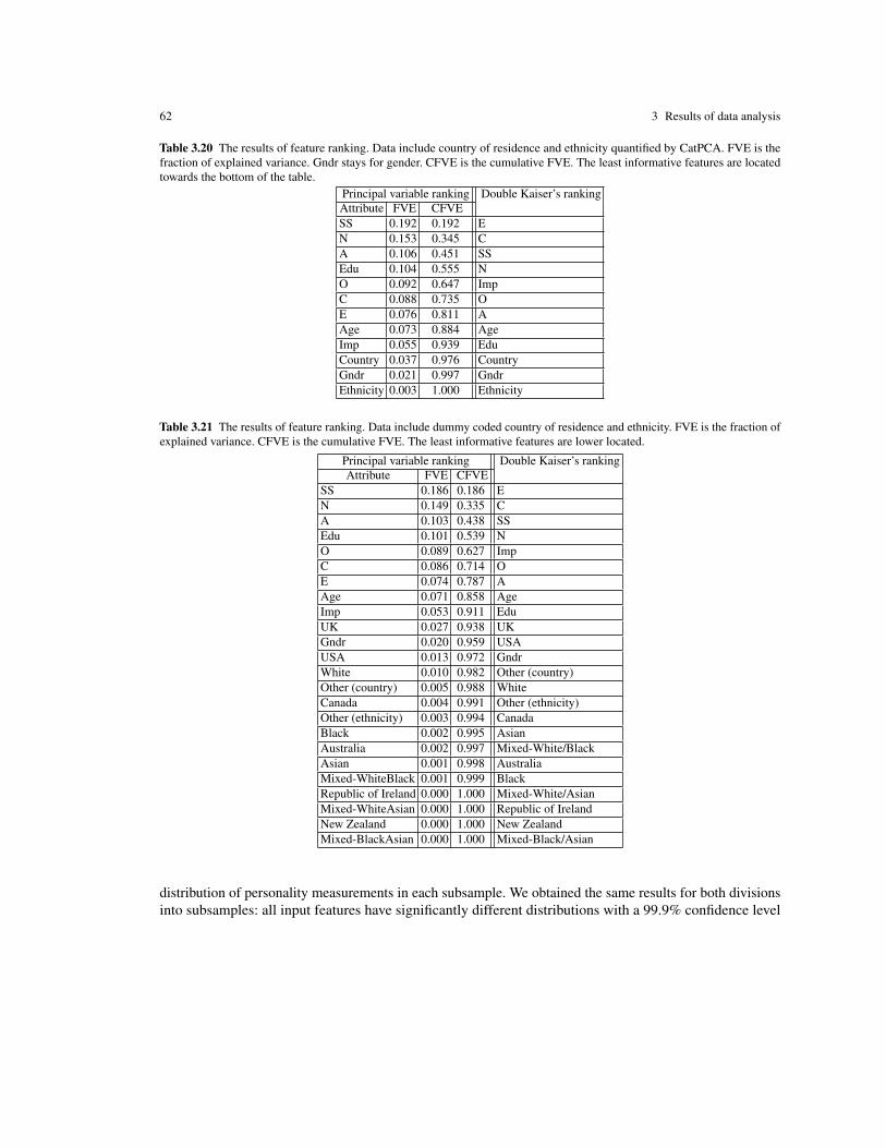
62 3 Results of data analysis
Table 3.20 The results of feature ranking. Data include country of residence and ethnicity quantified by CatPCA. FVE is thefraction of explained variance. Gndr stays for gender. CFVE is the cumulative FVE. The least informative features are locatedtowards the bottom of the table.
Principal variable ranking Double Kaiser’s rankingAttribute FVE CFVESS 0.192 0.192 EN 0.153 0.345 CA 0.106 0.451 SSEdu 0.104 0.555 NO 0.092 0.647 ImpC 0.088 0.735 OE 0.076 0.811 AAge 0.073 0.884 AgeImp 0.055 0.939 EduCountry 0.037 0.976 CountryGndr 0.021 0.997 GndrEthnicity 0.003 1.000 Ethnicity
Table 3.21 The results of feature ranking. Data include dummy coded country of residence and ethnicity. FVE is the fraction ofexplained variance. CFVE is the cumulative FVE. The least informative features are lower located.
Principal variable ranking Double Kaiser’s rankingAttribute FVE CFVE
SS 0.186 0.186 EN 0.149 0.335 CA 0.103 0.438 SSEdu 0.101 0.539 NO 0.089 0.627 ImpC 0.086 0.714 OE 0.074 0.787 AAge 0.071 0.858 AgeImp 0.053 0.911 EduUK 0.027 0.938 UKGndr 0.020 0.959 USAUSA 0.013 0.972 GndrWhite 0.010 0.982 Other (country)Other (country) 0.005 0.988 WhiteCanada 0.004 0.991 Other (ethnicity)Other (ethnicity) 0.003 0.994 CanadaBlack 0.002 0.995 AsianAustralia 0.002 0.997 Mixed-White/BlackAsian 0.001 0.998 AustraliaMixed-WhiteBlack 0.001 0.999 BlackRepublic of Ireland 0.000 1.000 Mixed-White/AsianMixed-WhiteAsian 0.000 1.000 Republic of IrelandNew Zealand 0.000 1.000 New ZealandMixed-BlackAsian 0.000 1.000 Mixed-Black/Asian
distribution of personality measurements in each subsample. We obtained the same results for both divisionsinto subsamples: all input features have significantly different distributions with a 99.9% confidence level

3.8 Selection of the best classifiers for the decade-based classification problem 63
for UK and non-UK subsamples and likewise for USA – non-USA subsamples. This means that the UK andnon-UK samples are biased, and similarly for the USA and non-USA samples.
Our goal is to predict the risk of drug consumption for an individual. This means that we have to considerindividual specific factors. Occupation within a specific country can be thought of as an important risk factor,but we do not have enough data for countries other than the UK and the USA because of the composition ofthe dataset: participants from the UK (1,044; 55.4%), the USA (557; 29.5%), Canada (87; 4.6%), Australia(54; 2.9%), New Zealand (5; 0.3%) and Ireland (20; 1.1%). A total of 118 (6.3%) came from a diversityof other countries, none of whom individually formed as much as 1% of the sample, or did not declare thecountry of location. Thus we exclude the ‘country’ feature from further study. As a result, we continue withthe 10 input features: Age, Edu, N, E, O, A, C, Imp, SS, and Gndr.
Table 3.22 The result of sparse PCA feature ranking. Data include country of residence and ethnicity quantified by CatPCA.
Step # of components Removed attributes1 5 Gndr and Ethnicity
2 4No removed attributes. The retained set of attributes: Age, Edu,
N, E, O, A, C, Imp, SS, and country
Table 3.23 The result of sparse PCA feature ranking. Data include dummy coded country of residence and ethnicity.
Step # of components Removed attributes
1 8Canada, Other (country), Australia, Republic of Ireland,
New Zealand, Mixed-White/Asian, White, Other (ethnicity),Mixed-White/Black, Asian, Black and Mixed-Black/Asian
2 5 Gndrr, UK and USA
3 4No removed attributes. The retained set of attributes: Age,
Edu, N, E, O, A, C, Imp, and SS
3.8 Selection of the best classifiers for the decade-based classification problem
The first step for risk evaluation is the construction of classifiers. We have tested the eight methods describedin the ‘Risk evaluation methods’ Section and selected the best one. The results of classifier selection arepresented in Table 3.24. This table shows that for all drugs except alcohol, cocaine and magic mushrooms,the sensitivity and specificity are greater than 70%, which is an unexpectedly high accuracy.
Recall that we have 10 input features: Age, Edu, N, E, O, A, C, Imp, SS, and Gndr; each of which isan important predictor for at least five drugs. However, there is no single most effective classifier whichuses all input features. The maximal number of attributes used is 6 out of 10 and the minimal number is 2.In Section 2.3.2 the best method is defined as the method which maximises the value of the minimum ofsensitivity and specificity. If the minimum of sensitivity and specificity is the same for several classifiers thenthe classifier with the maximal sum of the sensitivity and specificity is selected from these. Table 3.24 showsthe different sets of attributes which are used in the best user/non-user classifier for each different drug.
The use of a feature in the best classifier can be interpreted as ‘ranking by fact’. We note that this rankingby fact is very different from the other rankings presented in Tables 3.20 and 3.22. For example, in Tables 3.20

64 3 Results of data analysis
Table 3.24 The best results of the drug users classifiers (decade-based definition of users). Symbol ‘X’ means the used inputfeature. Results are calculated by LOOCV.
Target feature Classifier Age Edu N E O A C Imp SS Gndr Sn Sp Sum(%) (%) (%)
Alcohol LDA X X X X X 75.34 63.24 138.58Amphetamines DT X X X X X X 81.30 71.48 152.77Amyl nitrite DT X X X X 73.51 87.86 161.37Benzodiazepines DT X X X X X X 70.87 71.51 142.38Cannabis DT X X X X X X 79.29 80.00 159.29Chocolate kNN X X X X 72.43 71.43 143.86Cocaine DT X X X X X 68.27 83.06 151.32Caffeine kNN X X X X X 70.51 72.97 143.48Crack DT X X 80.63 78.57 159.20Ecstasy DT X X X 76.17 77.16 153.33Heroin DT X X X 82.55 72.98 155.53Ketamine DT X X X X X 72.29 80.98 153.26Legal highs DT X X X X X X 79.53 82.37 161.90LSD DT X X X X X X 85.46 77.56 163.02Methadone DT X X X X X 79.14 72.48 151.62MMushrooms DT X X 65.56 94.79 160.36Nicotine DT X X X X 71.28 79.07 150.35VSA DT X X X X X X 83.48 77.64 161.12
and 3.22 we see that Age is not one of the most informative measures, but it is used in the best classifiersfor 14 of the drugs. The second most used input feature is Gndr, which is regarded as non-informative bySparse PCA (Table 3.22) and as one of the least informative by other methods (Table 3.20). This means thatconsumption of these 10 drugs is Gndr dependent.
We have found some unexpected outcomes. For example, in the dataset the fraction of females who arealcohol users is greater than that fraction of males (Fig. 3.9) but a greater proportion of males consumecaffeine drinks (for example, coffee) (Fig. 3.10). The fraction of males who do not eat chocolate is greaterthan for females (Fig. 3.11). The conditional distributions for nicotine show the fraction of males who smokeis higher (Fig. 3.12).
Fig. 3.9 Conditional distribution for Gndr and alcohol

3.8 Selection of the best classifiers for the decade-based classification problem 65
Fig. 3.10 Conditional distribution for Gndr and caffeine
Fig. 3.11 Conditional distribution for Gndr and chocolate
The next most informative input features are E and SS which are used in the best classifiers for nine drugs.Features O, C, and Imp are used in the best classifiers for eight drugs. Features N and A are used in thebest classifiers for six drugs. Thus, personality factors are associated with drug use and each one impacts onspecific drugs. Finally, Edu is used in the best classifiers for five drugs (see Table 3.24).
To predict the usage of most drugs DT is the best classifier (see Table 3.24). LDA is the best classifierfor alcohol use with five input features, and has sensitivity 75.34% and specificity 63.24%. kNN is the bestclassifier for chocolate and caffeine users. These kNN classifiers use four features for chocolate and fivefeatures for caffeine.
The drugs can be separated into disjoint groups by the number of attributes used for the best classifiers:
• The group of classifiers with two input features contains classifiers for two drugs: crack and magicmushrooms. Both classifiers for this group use the E score.
• The group of classifiers with three input features includes classifiers for two drugs: ecstasy and heroin.Both classifiers in this group use Age and Gndr and do not use any NEO-FFI factors.
• The group of classifiers with four input features includes classifiers for three drugs: amyl nitrite, chocolate,and nicotine. All classifiers for this group use the C score.

66 3 Results of data analysis
Fig. 3.12 Conditional distribution for Gndr and nicotine
• The group of classifiers with five input features includes classifiers for five drugs: alcohol, cocaine, caffeine,ketamine, and methadone. All classifiers for this group use Age.
• The group of classifiers with six input features includes classifiers for six drug users: amphetamines,benzodiazepines, cannabis, legal highs, LSD, and VSA. All classifiers for this group use Age.
It is important to stress that the attributes which are not used in the best classifiers are not non-informative.For example, for ecstasy consumption the best classifier is based on Age, SS, and Gndr and has sensitivity76.17% and specificity 77.16%. There exists a DT for usage of the same drug based on Age, Edu, O, C, andSS, with sensitivity 77.23% and specificity 75.22%; a DT based on Age, Edu, E, O, and A, with sensitivity73.24% and specificity 78.22%; a LR classifier based on Age, Edu, O, C, Imp, SS, and Gndr, with sensitivity74.83% and specificity 74.52%; a kNN classifier based on Age, Edu, N, E, O, C, Imp, SS, and Gndr, withsensitivity 75.63% and specificity 75.75%. This means that for the risk evaluation of ecstasy usage all inputattributes are informative but the required information can be extracted from a smaller subset of the attributes.
The results presented in Table 3.24 were calculated by LOOCV. It should be stressed that different methodsof testing give rise to different values for sensitivity and specificity. Common methods include calculation oftest set errors (the holdout method), k-fold cross-validation, testing on the entire sample (if it is sufficientlylarge, the so-called ‘naıve’ method), random sampling, and many others. For example, a DT formed for theentire sample can have a sensitivity and specificity different from LOOCV [15]. For illustration, consider theDT for ecstasy, depicted in Fig. 3.13. It has sensitivity 78.56% and specificity 71.16%, calculated using thewhole sample. The results of LOOCV for a tree with the same choices are given in Table 3.24: sensitivity76.17% and specificity 77.16%.
The role of SS is very important for most of the party drugs. In particular, the risk of ecstasy consumptioncan be evaluated with high accuracy on the basis of Age, Gndr and SS (see Table 3.24, Fig. 3.13, and 3.27),and does not need the personality traits from the FFM.
3.9 Correlation pleiades of drugs
Consider correlations between drug usage for the year- and decade-based definitions (Fig. 3.7). It can be seenfrom Fig. 3.7 that the structure of these correlations for the year- and decade-based definitions of drug users isapproximately the same. We have found three groups of strongly correlated drugs, each containing several

3.9 Correlation pleiades of drugs 67
Fig. 3.13 Decision tree for ecstasy. Input features are: Age, SS, and Gndr. Non-terminal nodes are depicted with dashed border.Values of Age, SS, and Gndr are calculated by quantification procedures described in Section 2.2.2. The weight of each case ofusers class is 1.15 and of non-users class is 1. In column ‘Weighted’ normalizing weights are presented (the weight of each classis divided by sum of weights)
drugs which are pairwise strongly correlated. This means that drug consumption has a ‘modular structure’,and we have identified three modules:
• Crack, cocaine, methadone, and heroin;• Amphetamines, cannabis, cocaine, ketamine, LSD, magic mushrooms, legal highs, and ecstasy;• Methadone, amphetamines, cocaine and benzodiazepines.
This modular structure has a clear representation in the correlation graph, Fig. 3.7.
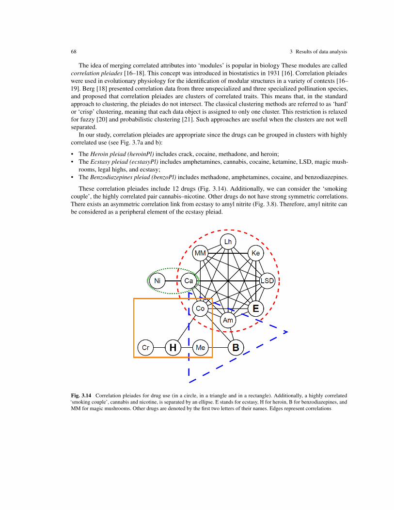
68 3 Results of data analysis
The idea of merging correlated attributes into ‘modules’ is popular in biology These modules are calledcorrelation pleiades [16–18]. This concept was introduced in biostatistics in 1931 [16]. Correlation pleiadeswere used in evolutionary physiology for the identification of modular structures in a variety of contexts [16–19]. Berg [18] presented correlation data from three unspecialized and three specialized pollination species,and proposed that correlation pleiades are clusters of correlated traits. This means that, in the standardapproach to clustering, the pleiades do not intersect. The classical clustering methods are referred to as ‘hard’or ‘crisp’ clustering, meaning that each data object is assigned to only one cluster. This restriction is relaxedfor fuzzy [20] and probabilistic clustering [21]. Such approaches are useful when the clusters are not wellseparated.
In our study, correlation pleiades are appropriate since the drugs can be grouped in clusters with highlycorrelated use (see Fig. 3.7a and b):
• The Heroin pleiad (heroinPl) includes crack, cocaine, methadone, and heroin;• The Ecstasy pleiad (ecstasyPl) includes amphetamines, cannabis, cocaine, ketamine, LSD, magic mush-
rooms, legal highs, and ecstasy;• The Benzodiazepines pleiad (benzoPl) includes methadone, amphetamines, cocaine, and benzodiazepines.
These correlation pleiades include 12 drugs (Fig. 3.14). Additionally, we can consider the ‘smokingcouple’, the highly correlated pair cannabis–nicotine. Other drugs do not have strong symmetric correlations.There exists an asymmetric correlation link from ecstasy to amyl nitrite (Fig. 3.8). Therefore, amyl nitrite canbe considered as a peripheral element of the ecstasy pleiad.
Fig. 3.14 Correlation pleiades for drug use (in a circle, in a triangle and in a rectangle). Additionally, a highly correlated‘smoking couple’, cannabis and nicotine, is separated by an ellipse. E stands for ecstasy, H for heroin, B for benzodiazepines, andMM for magic mushrooms. Other drugs are denoted by the first two letters of their names. Edges represent correlations
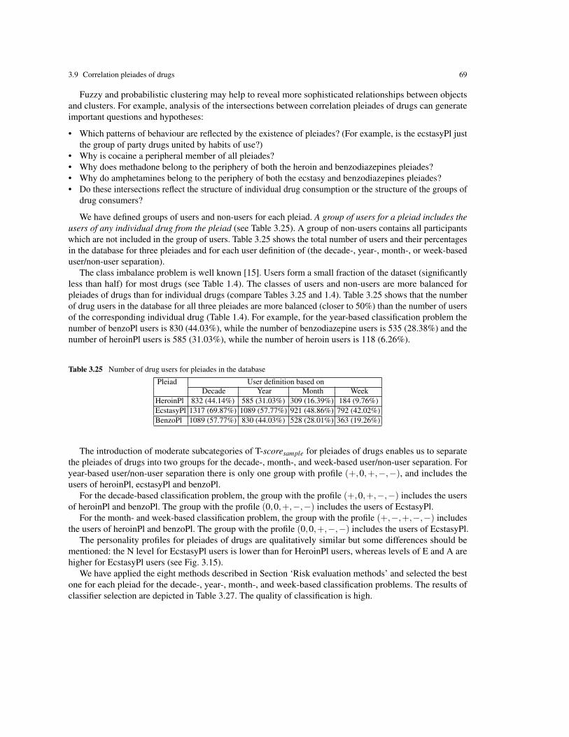
3.9 Correlation pleiades of drugs 69
Fuzzy and probabilistic clustering may help to reveal more sophisticated relationships between objectsand clusters. For example, analysis of the intersections between correlation pleiades of drugs can generateimportant questions and hypotheses:
• Which patterns of behaviour are reflected by the existence of pleiades? (For example, is the ecstasyPl justthe group of party drugs united by habits of use?)
• Why is cocaine a peripheral member of all pleiades?• Why does methadone belong to the periphery of both the heroin and benzodiazepines pleiades?• Why do amphetamines belong to the periphery of both the ecstasy and benzodiazepines pleiades?• Do these intersections reflect the structure of individual drug consumption or the structure of the groups of
drug consumers?
We have defined groups of users and non-users for each pleiad. A group of users for a pleiad includes theusers of any individual drug from the pleiad (see Table 3.25). A group of non-users contains all participantswhich are not included in the group of users. Table 3.25 shows the total number of users and their percentagesin the database for three pleiades and for each user definition of (the decade-, year-, month-, or week-baseduser/non-user separation).
The class imbalance problem is well known [15]. Users form a small fraction of the dataset (significantlyless than half) for most drugs (see Table 1.4). The classes of users and non-users are more balanced forpleiades of drugs than for individual drugs (compare Tables 3.25 and 1.4). Table 3.25 shows that the numberof drug users in the database for all three pleiades are more balanced (closer to 50%) than the number of usersof the corresponding individual drug (Table 1.4). For example, for the year-based classification problem thenumber of benzoPl users is 830 (44.03%), while the number of benzodiazepine users is 535 (28.38%) and thenumber of heroinPl users is 585 (31.03%), while the number of heroin users is 118 (6.26%).
Table 3.25 Number of drug users for pleiades in the database
Pleiad User definition based onDecade Year Month Week
HeroinPl 832 (44.14%) 585 (31.03%) 309 (16.39%) 184 (9.76%)EcstasyPl 1317 (69.87%) 1089 (57.77%) 921 (48.86%) 792 (42.02%)BenzoPl 1089 (57.77%) 830 (44.03%) 528 (28.01%) 363 (19.26%)
The introduction of moderate subcategories of T-scoresample for pleiades of drugs enables us to separatethe pleiades of drugs into two groups for the decade-, month-, and week-based user/non-user separation. Foryear-based user/non-user separation there is only one group with profile (+,0,+,−,−), and includes theusers of heroinPl, ecstasyPl and benzoPl.
For the decade-based classification problem, the group with the profile (+,0,+,−,−) includes the usersof heroinPl and benzoPl. The group with the profile (0,0,+,−,−) includes the users of EcstasyPl.
For the month- and week-based classification problem, the group with the profile (+,−,+,−,−) includesthe users of heroinPl and benzoPl. The group with the profile (0,0,+,−,−) includes the users of EcstasyPl.
The personality profiles for pleiades of drugs are qualitatively similar but some differences should bementioned: the N level for EcstasyPl users is lower than for HeroinPl users, whereas levels of E and A arehigher for EcstasyPl users (see Fig. 3.15).
We have applied the eight methods described in Section ‘Risk evaluation methods’ and selected the bestone for each pleiad for the decade-, year-, month-, and week-based classification problems. The results ofclassifier selection are depicted in Table 3.27. The quality of classification is high.

70 3 Results of data analysis
Table 3.26 Statistically significant differences of means for groups of users and non-users for each pleiad for decade- year-,month-, and week-based classification problem. The symbol ‘⇓ ’corresponds to a significant difference where the mean in theusers group is less than the mean in the non-users group, and the symbol ‘⇑’ corresponds to a significant difference where themean in the users group is greater than the mean in the non-users group. Empty cells corresponds to insignificant differences.The difference is considered to be significant if the p-value is less than 0.01)
Pleiades od drugs N E O A CThe decade-based user/non-user separation
HeroinPl, EcstasyPl, BenzoPl ⇑ ⇑ ⇓ ⇓The year-based user/non-user separation
HeroinPl, EcstasyPl, BenzoPl ⇑ ⇑ ⇓ ⇓The month-based user/non-user separation
HeroinPl, EcstasyPl ⇑ ⇑ ⇓ ⇓BenzoPl ⇑ ⇓ ⇑ ⇓ ⇓
The week-based user/non-user separationHeroinPl, BenzoPl ⇑ ⇓ ⇑ ⇓ ⇓EcstasyPl ⇑ ⇑ ⇓ ⇓
The classification results are excellent for each pleiad for the decade-, year-, month, and week-basedproblems. We can compare the classifiers for one pleiad and for different problems (see Table 3.27). Forexample:
• The best classifier for ecstasyPl for the year-based user/non-user separation is a DT with seven attributesand has sensitivity 80.65% and specificity 80.72%;
• The best classifier for heroinPl for the month-based user/non-user separation is a DT with five attributesand has sensitivity 74.18% and specificity 74.11%;
• The best classifier for benzoPl for the week-based user/non-user separation is a DT with five attributes andhas sensitivity 75.10% and specificity 75.76%.
Table 3.27 The best results for classifiers of the pleiad users. Symbol ‘X’ means input feature used in the best classifier.Sensitivity (Sn) and Specificity (Sp) were calculated by LOOCV.
Pleiades Classifier Age Edu N E O A C Imp SS Gndr # Sn Sp Sumof drugs (%) (%) (%)
The decade-based user/non-user separationHeroinPl DT X X X X 4 71.23 78.85 150.07EcstasyPl DT X X X X X X 6 80.63 79.80 160.44BenzoPl DT X X X X X 5 73.37 72.45 145.82
The year-based user/non user-separationHeroinPl DT X X X X 4 73.69 71.80 145.49EcstasyPl DT X X X X X X X 7 80.65 80.72 161.37BenzoPl DT X X X X 4 73.93 73.98 147.91
The month-based user/non user-separationHeroinPl DT X X X X X 5 74.18 74.11 148.29EcstasyPl PDFE X X X X X X X X 8 79.34 79.50 158.83BenzoPl DT X X X X 4 73.18 73.11 146.28
The week-based user/non user-separationHeroinPl DT X X X X X X X X 8 75.84 73.91 149.75EcstasyPl LR X X X X X X X X 8 77.68 77.78 155.45BenzoPl DT X X X X X 5 75.10 75.76 150.86

3.9 Correlation pleiades of drugs 71
Fig. 3.15 Average personality profiles for drug pleiades for the month- and week-based user/non-user separation (T-scoresamplewith respect to the sample means)
Comparison of Tables 3.24 and 3.27 shows that the best classifiers for the ecstasy and benzodiazepinespleiades are more accurate than the best classifiers for the consumption of the ‘central’ drugs of the pleiades,ecstasy and benzodiazepines respectively, even for the decade-based user definition. Classifiers for heroinPlmay have slightly worse accuracy but these classifiers are more robust because they solve classificationproblems which have more balanced classes. All other classifiers for pleiades of drugs are more robust too forthe same reasons, for all pleiades and definitions of users.
Tables 3.24 and 3.27 for the decade-based user definition show that most of the classifiers for pleiades usemore input features than the classifiers for individual drugs. We can see from these tables that the accuraciesof the classifiers for pleiades and for individual drugs do not differ drastically, but the use of a greater numberof input features suggests more robust classifiers.
It is important to remark that pleiades are usually assumed to be disjoint. We have considered pleiadeswhich are named by the central drug and the peripheral drugs can be shared. For example, the heroin andecstasy pleiades have cocaine as an intersection. This approach corresponds to the concept of ‘soft clustering’.

72 3 Results of data analysis
3.10 Overoptimism problem
The best machine learning methods selected give impressive solutions for the user/non-user classificationproblems. Nevertheless, the procedure of selection has used the same data as the training process: we havetested each method by LOOCV. Such an approach could produce so-called overoptimism: the cross-validationerrors of the best method on the same set, which was used for the method selection, may be underestimated.
To demonstrate that the data of Tables 3.24 and 3.27 are valid for generalisation errors and samples we havenever seen before, we may need additional validation on a large hold out sample, which was not compromisedby its usage in the method selection. We do not have an additional large sample and splitting the existingsample into a training set (for training and cross-validation in method selection) and a validation set (forvalidation of the best method) will decrease the statistic power of analysis [22].
Following [24], high performance on the test sample does not guarantee high performance on futuresamples, things do change and there is always a chance that a variable and its relationships will be different infuture samples. Selection of the best models and best sets of ‘dominant variables’ can damage robustness ofthe model to future variations.
The idea of stability of the model can significantly help in the testiong of classifiers [23]. In the process ofcross-validation we can test additionally stability of the model and answer the questions:
• How many examples change their class in cross-validation (we can calculate the number for each transitionbetween classes: class A→ class B, etc.). This is classification stability.
• How many qualitatively different models (for example, decision trees with different structure) weregenerated in cross-validation. This is structural stability.
We can also extract the set of examples with unstable classification and study this set separately.Hand [25] clearly demonstrated that ‘simple methods typically yield performance almost as good as more
sophisticated methods, to the extent that the difference in performance may be swamped by other sources ofuncertainty that generally are not considered in the classical supervised classification paradigm.’
Therefore, let us consider the results of the best methods (Tables 3.24 and 3.27) as an upper border of thepossible classifier performance and apply the simple linear discriminant method. This method is robust andleaves no space for overoptimism if the samples are sufficiently large and there is no multicollinearity. Wehave also analysed the classification stability of the linear discriminant in cross-validation.
Multicollinearity means strong linear dependence between input attributes. This makes the model verysensitive to fluctuations in data is an important source of instability of classifiers. The standard measure ofmulticollinearity is the condition number of the correlation matrix, that is the ratio κ = λmax/λmin, where λmaxand λmin are the maximal and the minimal eigenvalues of this matrix. Collinearity with κ < 10 is consideratedas ‘modest’ collinearity [26].
Eigenvalues of the correlation matrix between the seven psychological traits are:
λi = 2.267,1.809,0.887,0.678,0.548,0.468,0.342; κ = λmax/λmin = 6.628.
Eigenvalues of the correlation matrix between the ten attributes (quantified) including the seven psychologicaltraits, Age, Edu and Gndr are:
λi = 2.595,1.867,1.111,0.980,0.814,0.757,0.599,0.524,0.427,0.327; κ = λmax/λmin = 7.945.
We can see that there is no strong multicollinearity despite the existence of significant and not smallcorrelations between psychological traits (see Tables 3.9 and 3.10). Three correlation coefficients, betweenthe N and E scores, between the O and SS scores and between the Imp and SS scores exceed 0.4 in

3.11 User/non-user classification by linear discriminant for ecstasy and heroin 73
absolute value. Absolute values of correlation coefficients above 0.4 are sometimes interpreted as indicatinga multicollinearity problem. This heuristic rule is not rigorous but existence of such correlations rises asuspicion of multicollinearity and it is necessary to apply a stronger test. We have calculated the conditionnumber and it is sufficiently low to exclude strong multicollinearity. In the next section we have demonstratedthat Fisher’s linear discriminant is sufficiently robust and works stably for these values of κ in our database.
3.11 User/non-user classification by linear discriminant for ecstasy and heroin
Fisher [4] defined the linear discriminant (LD) as a linear function of attributes, for which the ratio of thedifference between classes to the standard deviation within classes is maximal (see, for example, the score2.9). We have used the classical formula for the LD direction (2.10). The selection threshold (intercept) Θ isdefined by the balance condition Sn=Sp.
Linear discriminants separate users from non-users by linear inequalities:
D(z) =Θ +∑cizi > 0 (3.2)
for users and ≤ 0 for non-users, where Θ are the thresholds (intercepts), zi are the attributes, and ci are thecoefficients.
Tables A.5-A.8 in the Appendix contain the coefficients ci of the linear discriminants for user/nonuserseparation in 10-dimensional space (7 psychological attributes, Age, Edu, and Gndr). The attributes in thesetables are quantified and transformed to z-scores with zero mean and unit variance (positive values of the Gndrz-score corresponds to female). The last rows of the tables include the standard deviation of the coefficientsin LOOCV. For the 7-dimensional space of psychological attributes (T-scores), the coefficients of lineardiscriminants are presented in Tables A.13-A.16.
Performance of linear discriminants in user/non-user separation is evaluated by several methods (TablesA.9–A.12 for the 10-dimensional data space and Tables A.17–A.20 for the 7-dimensional space of T-scores ofpsychological attributes). First of all, we have calculated the linear discriminant using the whole sample (seeTables A.5–A.8) and find all of their errors. For each solution of the classification problem we have severalnumbers, P (positive), the number of samples recognised as positive, and N (negative), the number of samplesrecognised as negative. P+N is the total number of samples. P=TP+FP (True Positive plus False Positive)and N=TN+FN (True Negative plus False Negative). Sensitivity is Sn=TP/(TP+FN)×100% and Specificity isSp=TN/(TN+FP)×100%. Accuracy is Acc=(TP+TN)/(P+N)×100%.
We have calculated these performance indicators for the total sample and for the LOOCV procedure.In LOOCV the linear discriminant is calculated for the set of all samples excluding the example left outfor testing. The test was performed for all samples with the corresponding redefining of Sn, Sp, and Acc.In LOOCV the linear discriminants are calculated for each test example. Each of these discriminants is aseparate classification model. Stability of classification can be measured by the number of examples whichchange their class at least once. We have taken the basis model for the total sample and found how many TPexamples of this model became FN examples of a LOOCV model at least once. This number measured in %of TP+FP of the basic model is TP→FN. Analogously, we have defined FP→TN, TN→FP, and FN→TP. Thelast two numbers are measured in % of TN+FN of the basic model.
In this section we have analysed performance of linear discriminants for two drugs, ecstasy and heroin.They are typical (and central) elements of two pleiades, groups of drugs with correlated drug usage. Thedifferences between them might tell us a story about different types of drug users.
74 3 Results of data analysis
Table 3.28 Coefficients of the linear discriminant for the ecstasy user/non-user separation and decade-, year-, month-, andweek-based definition of users (10 attributes)
Period Θ Age Edu N E O A C Imp SS GndrDecade -0.171 -0.631 -0.188 0.053 0.018 0.351 -0.065 -0.210 -0.088 0.559 -0.265Year -0.464 -0.782 -0.101 -0.015 0.099 0.238 -0.025 -0.173 -0.004 0.453 -0.275Month -0.633 -0.820 0.047 -0.139 0.093 0.284 -0.123 -0.165 -0.028 0.328 -0.257Week -0.779 -0.697 0.077 -0.115 0.161 0.545 -0.093 -0.252 0.217 0.230 -0.022
SD ≤ 0.018 ≤ 0.002 ≤ 0.003 ≤ 0.004 ≤ 0.004 ≤ 0.003 ≤ 0.003 ≤ 0.003 ≤ 0.004 ≤ 0.005 ≤ 0.003
Table 3.29 Performance and stability of the linear discriminant for the ecstasy user/non-user separation and decade-, year-,month-, and week-based definition of users (10 attributes). All indicators are in %.
Total sample LOOCV Stability indicatorsPeriod Sn Sp Acc Sn Sp Acc TP→FN FN→TP FP→TN TN→FP
Decade 74.4 74.7 74.6 74.2 74.3 74.2 0.3 0.7 0.5 0.4Year 75.4 75.7 75.6 75.0 75.6 75.4 0.2 0.6 0.8 0.3Month 72.5 72.4 72.4 71.3 72.3 72.1 1.7 1.3 1.2 1.2Week 72.6 71.5 71.5 67.9 71.4 71.2 3.6 8.3 2.4 5.3
Table 3.30 Coefficients of the linear discriminant for the heroin user/non-user separation and decade-, year-, month-, andweek-based definition of users (10 attributes)
Period Θ Age Edu N E O A C Imp SS GndrDecade -0.615 -0.210 -0.370 0.413 -0.211 0.477 -0.265 -0.029 0.222 0.381 -0.332Year -0.849 -0.584 -0.168 0.352 -0.252 0.222 -0.275 0.014 0.216 0.359 -0.378Month -1.037 -0.560 -0.371 0.181 -0.350 0.159 -0.397 0.016 0.368 0.154 -0.226Week -1.096 -0.386 -0.077 0.467 -0.255 0.184 -0.412 0.013 0.437 -0.077 -0.400
SD ≤ 0.005 ≤ 0.004 ≤ 0.004 ≤ 0.004 ≤ 0.004 ≤ 0.004 ≤ 0.004 ≤ 0.004 ≤ 0.005 ≤ 0.006 ≤ 0.003
Table 3.31 Performance and stability of the linear discriminant for the heroin user/non-user separation and decade-, year-,month-, and week-based definition of users (10 attributes). All indicators are in %.
Total sample LOOCV Stability indicatorsPeriod Sn Sp Acc Sn Sp Acc TP→FN FN→TP FP→TN TN→FP
Decade 70.8 69.9 70.0 68.4 69.8 69.7 2.8 6.1 1.3 2.2Year 73.7 73.7 73.7 70.3 73.6 73.4 2.5 2.5 2.1 2.3Month 79.2 77.6 77.7 69.8 77.5 77.2 9.4 7.5 3.2 3.8Week 79.3 80.1 80.1 65.5 80.0 79.8 6.9 6.9 4.6 4.8
Coefficients of LD can be used for indication of how a change in an attribute value will affect the valueof D(z) under the condition that the values of all other attributes do not change. It is possible to change oneattribute without changing other attributes because there is no strong multicollinearity. The most interestingin this ranking for the Tables 3.28 and 3.30 is the essential difference between ranking for ecstasy and forheroin user/non-user discriminants.
Comparison of Tables 3.28 and 3.30 immediately gives a result. The coefficients of LD for ecstasy andheroin have significant differences: for ecstasy, the effect of Imp is less than for heroin (and can even havedifferent sign), whereas the effect of SS is bigger for ecstasy. For ecstasy, the coefficients of A have smallervalues than the coefficients of C. For heroin the situation is opposite: C has much smaller coefficient than A(and can even have the opposite sign). Also, coefficients of N for ecstasy are smaller than for heroin and canhave different sign. Edu has negative coefficients for heroin with bigger values (it ‘prevents’ usage of heroin),

3.11 User/non-user classification by linear discriminant for ecstasy and heroin 75
whereas for ecstasy the influence of Edu is smaller and can have opposite signs (for week- and month-baseddefinition of usage). Coefficients of E are positive for the ecstasy user/non-user separation and negative for theheroin user/non-user separation. Age has large negative coefficients both for ecstasy and heroin but for ecstasythey are 1.5–2 times bigger. For example, for the month-based definition of users the ranking of variables is:
• For ecstasy: Age⇓ , SS⇑, O⇑, Gndr⇓ , C⇓, N⇓, A⇓, E⇑, Edu⇑, Imp⇓;• For heroin: Age⇓, A⇓, Edu⇓, Imp⇑, E⇓, Gndr⇓ , N⇑, O⇑, SS⇑, C⇑.
The arrows ⇑ ⇓ here indicates the sign of the effect of the attribute in the user/non-user separation (and not theshift of the mean as it was in previous sections): for positive coefficients it is ⇑ and for negative coefficients itis ⇓. The difference between heroin and ecstasy discriminants is impressive. The most important five attributesfor ecstasy user/non-user discrimination have only one attribute in common with the top five attributes ofheroin user/non-user discrimination (Age). We invite the reader to pay attention to the different signs ofcoefficients of some of the attributes for the ecstasy and heroin linear user/non-user discrimination in this case:C, N, E, and Imp. For most of these attributes, the traditional expectation is well-known: C⇓, N⇑, Imp⇑ (atleast, for illegal drugs). The values of the coefficients with unexpected signs are relatively small, the attributeswith these values are ranked as less important, but the expectation is not met in any case: we can state that itis a wrong assumption that high N and Imp are predictors for ecstasy use, and it is also wrong that low C is apredictor for heroin use.
If we do not use Age, Edu, and Gndr, then the difference of the predictors persists (Tables 3.32 and 3.33):for ecstasy LD the most important attribute becomes SS, then O and C. The attributes Imp, A, N, and E havesmaller coefficients, and for Imp, E, and N the sign of the coefficients depends on recency of usage. Forheroin C seems to be less important than other attributes.
The ranking of these seven psychological attributes for the same month-based user/non-user discriminationlooks similar:
• For ecstasy: SS⇑, O⇑, C⇓, N⇓, A⇓, Imp⇓, E⇑;• For heroin: SS⇑, A⇓ , E⇓ , Imp⇑, N⇑, O⇑, C⇓ .
The reader should note the opposite signs of N, E, and Imp for the ecstasy and heroin user/non-userdiscriminants in this case. The only big jump from the 10-attribute ranking is the change of rank of SS forheroin user/non-user discrimination. We believe that this is because of large negative correlations between SSand Age, which is important for classification but not available in the seven-attribute model. Again, the upperfour variables for ecstasy user/non-user discrimination have only one attribute in common with the top fourattributes of heroin user/non-user discrimination (SS).
Table 3.32 Coefficients of the linear discriminant for ecstasy user/non-user separation, for the decade-, year-, month-, andweek-based definition of users (7 attributes).
Period Θ N E O A C Imp SSDecade -35.896 0.045 -0.017 0.407 -0.085 -0.342 -0.156 0.827Year -42.579 -0.019 0.078 0.373 -0.045 -0.356 -0.096 0.846Month -27.572 -0.169 0.101 0.462 -0.191 -0.354 -0.139 0.752Week -60.127 -0.095 0.168 0.695 -0.128 -0.355 0.242 0.528
SD ≤ 0.565 ≤ 0.004 ≤ 0.005 ≤ 0.004 ≤ 0.004 ≤ 0.004 ≤ 0.005 ≤ 0.006
Employment of simple LDA demonstrates that users of ecstasy and heroin differ significantly, and users ofdifferent groups of drugs should be studied separately. The hypothesis that drug usage is associated with N⇑,

76 3 Results of data analysis
Table 3.33 Coefficients of the linear discriminant for heroin user/non-user separation, for the decade-, year-, month-, andweek-based definition of users (7 attributes).
Period Θ N E O A C Imp SSDecade -55.851 0.381 -0.283 0.526 -0.322 -0.124 0.249 0.563Year -44.733 0.361 -0.327 0.368 -0.397 -0.108 0.218 0.641Month -30.020 0.302 -0.409 0.232 -0.499 -0.107 0.345 0.555Week -37.099 0.548 -0.325 0.265 -0.547 -0.069 0.389 0.261
SD ≤ 0.523 ≤ 0.004 ≤ 0.004 ≤ 0.005 ≤ 0.004 ≤ 0.005 ≤ 0.006 ≤ 0.007
A⇓, and C⇓ seems plausible at first glance, but appears to be an oversimplification. Such an analysis, and aneven more detailed consideration using all definitions of drug use, is possible for every pair of drugs (andfor four groups of drugs) on the basis of the linear discriminant coefficients presented in Tables A.5-A.8 andA.13-A.16.
The difference between linear discriminant directions can be evaluated by measuring the angles betweenthem. For each drug, we calculate the angles between linear discriminant directions for all definition of usersand the direction for the decade-based definition of users. These angles are significantly smaller than theangles between the linear discriminant directions for the same recency of use and different drugs (Fig. 3.16).
Fig. 3.16 Angles between directions of linear discriminants for user/non-user classification for ecstasy and heroin. Two typesof angles are presented: between the discriminant directions for all periods and the discriminant vector for the decade-baseddefinitions of users for both drugs, and angles between directions of linear discriminants for ecstasy and heroin (and the sameperiods). For convenience, both cosines of angles (a, b) and angles in degrees (c, d) are presented
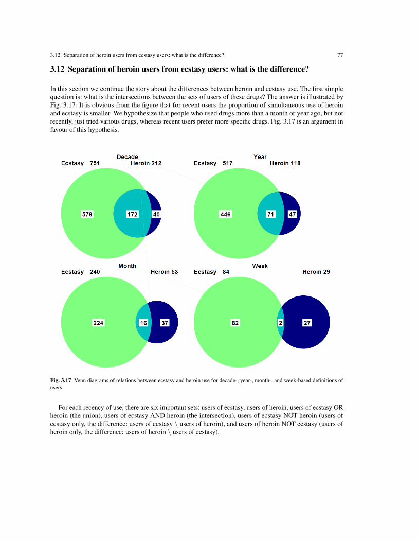
3.12 Separation of heroin users from ecstasy users: what is the difference? 77
3.12 Separation of heroin users from ecstasy users: what is the difference?
In this section we continue the story about the differences between heroin and ecstasy use. The first simplequestion is: what is the intersections between the sets of users of these drugs? The answer is illustrated byFig. 3.17. It is obvious from the figure that for recent users the proportion of simultaneous use of heroinand ecstasy is smaller. We hypothesize that people who used drugs more than a month or year ago, but notrecently, just tried various drugs, whereas recent users prefer more specific drugs. Fig. 3.17 is an argument infavour of this hypothesis.
Fig. 3.17 Venn diagrams of relations between ecstasy and heroin use for decade-, year-, month-, and week-based definitions ofusers
For each recency of use, there are six important sets: users of ecstasy, users of heroin, users of ecstasy ORheroin (the union), users of ecstasy AND heroin (the intersection), users of ecstasy NOT heroin (users ofecstasy only, the difference: users of ecstasy \ users of heroin), and users of heroin NOT ecstasy (users ofheroin only, the difference: users of heroin \ users of ecstasy).

78 3 Results of data analysis
The intersection of heroin and ecstasy users is sometimes large, so the discrimination task is a non-standardclassification. At least, the standard TPR (Sn) and TNR (Sp) do not make much sense. Let us consider abinary classification rule which separates all users of ecstasy OR heroin into two classes: E and H. We willconsider an example from the set of users of heroin OR ecstasy to be FE (‘false ecstasy’) if it is a non-user ofecstasy classified as a user of ecstasy (or, which is the same, a user of heroin but NOT ecstasy classified asa user of ecstasy). Analogously, an example is considered as FH (‘false heroin’) if it is non-user of heroinclassified as a user of heroin. In the Tables 3.34 we use an unusual measures of classification accuracy: TrueEcstasy Rate (TER) (correctly recognised fraction of users of ecstasy NOT heroin) and True Heroin Rate(THR) (correctly recognised fraction of users of heroin NOT ecstasy). We do not identify the case when auser of both drugs is recognised as a user of one them as an error:
TER =# correctly recognised users of ecstasy NOT heroin
# users of ecstasy NOT heroin;
THR =# correctly recognised users of heroin NOT ecstasy
# users of heroin NOT ecstasy.
The descriptive statistics for seven traits (FFM, Imp, and SS) are presented in Table 3.34 (compare to Table3.1). We can see that for ecstasy – heroin discrimination the best classifier with one attribute is N. Moreover,differences between means of ecstasy users and heroin users are statistically significant with confidence level99% for N and A, for all definitions of users, for Imp for decade-based and month-based definitions, and forE for all definitions excluding the decade-based one. This difference is obvious in the graphs of mean valuesof N, E, A, and Imp for ecstasy and heroin users shown in Fig. 3.19.
We have employed LDA for separation of ecstasy users from heroin users. We have applied the formula(2.10) for the linear discriminant direction with covariance matrices for ecstasy users and heroin userscalculated for the month-based definition of users. The intercept Θ was calculated for the most balancedseparation measured by TER and THR.
The ranking of attributes for the month-based ecstasy users / heroin users separation, based on the size ofthe coefficients of the linear discriminant, is:
N, E, A, Imp, SS, C, O (7 attributes).
It is important to note that the values of the coefficients of N, E, A, and Imp do not differ much and for SS, C,and O the coefficients are much smaller.
For 10 attributes the ranking by the linear discriminant coefficients is:
Edu, Imp, A, N, E, C, Gndr, SS, O, Age.
Again, for the leading group of attributes, Edu, Imp, A, N, and E, the coefficients decay slowly, and for theother attributes are much smaller. These observations, together with analysis of attribute means (Fig. 3.19),convinces us that the main and statistically significant differences between ecstasy users and heroin users arein Edu, Imp, A, N, and E.
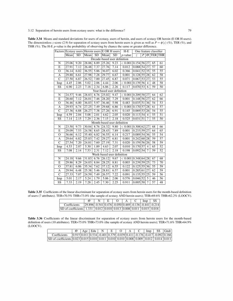
3.12 Separation of heroin users from ecstasy users: what is the difference? 79
Table 3.34 Means and standard deviations for users of ecstasy, users of heroin, and users of ecstasy OR heroin (E OR H users).The dimensionless z-score (2.9) for separation of ecstasy users from heroin users is given as well as P = φ(z) (%), TER (%), andTHR (%). The H-E p-value is the probability of observing by chance the same or greater difference.
Factors Ecstasy users Heroin users E OR H users H-E One feature classifierMean SD Mean SD Mean SD p-value z P Θ TER THR
Decade-based user definitionN 25.06 9.20 28.06 8.89 25.26 9.23 < 0.001 0.154 56 27 65 61E 27.91 7.12 26.48 7.37 27.76 7.14 0.012 0.088 54 27 57 60O 36.14 6.02 36.55 5.86 36.07 6.02 0.366 0.041 52 35 55 55A 29.88 6.61 27.98 7.28 29.77 6.67 0.001 0.128 55 28 62 58C 27.50 6.87 26.52 7.00 27.45 6.87 0.071 0.067 53 27 53 55
Imp 4.45 2.06 5.02 2.06 4.44 2.06 < 0.001 0.139 56 4 48 58SS 6.90 2.23 7.18 2.34 6.86 2.26 0.117 0.070 53 6 59 50
Year-based user definitionN 24.57 9.46 28.83 8.76 25.02 9.47 < 0.001 0.209 58 27 64 62E 28.60 7.12 26.01 7.46 28.20 7.29 0.001 0.148 56 27 62 66O 36.46 6.00 36.03 5.97 36.46 5.98 0.483 0.035 51 36 54 53A 29.93 6.74 27.25 7.49 29.68 6.86 < 0.001 0.170 57 28 61 57C 27.36 6.88 26.27 7.38 27.26 6.91 0.145 0.069 53 26 54 55
Imp 4.59 2.04 5.08 2.01 4.62 2.05 0.020 0.113 54 4 55 51SS 7.14 2.15 7.29 2.36 7.15 2.18 0.525 0.031 51 7 55 50
Month-based user definitionN 23.50 9.73 30.04 8.76 24.32 9.80 < 0.001 0.308 62 27 68 66E 29.09 7.53 24.58 8.65 28.43 7.89 0.001 0.233 59 27 64 65O 36.66 6.12 35.40 6.82 36.55 6.14 0.217 0.089 54 36 55 54A 29.64 6.82 25.83 7.42 29.27 6.81 0.001 0.242 60 28 59 57C 27.54 7.20 24.81 7.60 27.19 7.31 0.020 0.159 56 26 58 59
Imp 4.53 2.07 5.30 1.89 4.63 2.07 0.010 0.170 57 4 65 52SS 7.08 2.14 7.53 2.31 7.12 2.18 0.198 0.092 54 7 59 52
Week-based user definitionN 24.18 9.66 31.83 6.76 26.12 9.67 < 0.001 0.348 64 28 67 68E 29.86 8.29 24.03 8.84 28.25 8.81 0.003 0.239 59 25 73 70O 37.81 6.06 35.34 7.62 37.12 6.55 0.122 0.125 55 36 55 59A 29.94 6.48 25.38 5.46 28.81 6.57 0.001 0.285 61 27 62 59C 27.33 7.07 24.59 7.49 26.57 7.22 0.091 0.135 55 25 59 56
Imp 5.01 2.17 5.24 1.79 5.06 2.06 0.576 0.046 52 5 46 56SS 7.33 2.19 7.28 2.45 7.30 2.25 0.911 0.005 50 7 57 48
Table 3.35 Coefficients of the linear discriminant for separation of ecstasy users from heroin users for the month-based definitionof users (7 attributes). TER=70.5% THR=73.0% (the sample of ecstasy AND heroin users); TER=69.6% THR=62.2% (LOOCV).
Θ N E O A C Imp SSCoefficients 29.896 -0.541 0.476 -0.050 0.469 -0.136 -0.441 -0.214
SD of coefficients 1.331 0.012 0.010 0.013 0.008 0.011 0.015 0.018
Table 3.36 Coefficients of the linear discriminant for separation of ecstasy users from heroin users for the month-baseddefinition of users (10 attributes). TER=75.0% THR=73.0% (the sample of ecstasy AND heroin users); TER=71.6% THR=64.9%(LOOCV).
Θ Age Edu N E O A C Imp SS GndrCoefficients 0.915 0.011 0.534 -0.401 0.379 -0.039 0.411 -0.176 -0.417 -0.092 0.166
SD of coefficients 0.023 0.015 0.010 0.011 0.010 0.010 0.008 0.009 0.012 0.014 0.011

80 3 Results of data analysis
Fig. 3.18 Distribution of ecstasy (NOT heroin) users, heroin (NOT ecstasy) users, and heroin AND ecstasy users in various ageand education groups
3.13 Significant difference between benzodiazepines, ecstasy, and heroin
Analysis of differences between various groups of drug users can be extended to all pairs of drugs. Let usadd for investigation the centre of third pleiad, benzodiazepines. The relations between groups of users ofbenzodiazepines, ecstasy and heroin is shown in Fig. 3.20.
In Fig. 3.21 the mean values of personality traits N, E, O, A, Imp, SS are given with 95% CI for groups ofbenzodiazepines, ecstasy, and heroin users, and different recency of use. (C is not given because the differencein C between different groups of drug users is insignificant.)

3.13 Significant difference between benzodiazepines, ecstasy, and heroin 81
Fig. 3.19 Mean values with their 95% confidence intervals for significantly different psychological traits of ecstasy and heroinusers: (a) N, (b) E, (c) A, (d) Imp
Table 3.37 p-values of differences of mean values for benzodiazepines (benzos), ecstasy and heroin for all definitions of users.
Factors Benzos and ecstasy Benzos and heroin Ecstasy and heroinDecade Year Month Week Decade Year Month Week Decade Year Month Week
N 0.003 <0.001 <0.001 <0.001 0.021 0.088 0.322 0.188 <0.001 <0.001 <0.001 <0.001E 0.007 <0.001 <0.001 <0.001 0.443 0.275 0.189 0.590 0.012 0.001 0.001 0.003O 0.045 0.058 0.035 0.002 0.024 0.629 0.898 0.921 0.366 0.483 0.217 0.122A 0.697 0.128 0.141 0.150 0.002 0.007 0.010 0.006 0.001 <0.001 0.001 0.001C 0.439 0.943 0.412 0.557 0.021 0.135 0.052 0.146 0.071 0.145 0.020 0.091
Imp 0.315 0.520 0.457 0.172 <0.001 0.007 0.028 0.099 <0.001 0.020 0.010 0.576SS <0.001 0.001 0.081 0.009 <0.001 0.011 0.025 0.139 0.117 0.525 0.198 0.911
We can see from Table 3.37 that mean values in the groups of benzodiazepines and ecstasy users arestatistically significantly different with confidence level 95% for N (higher for benzodiazepines) and E (higherfor ecstasy) for all definition of users, for O (higher for ecstasy) for all definitions of users excluding theyear-based, and for SS (higher for ecstasy) for all definitions excluding the month-based. Benzodiazepinesand heroin are statistically significantly different with confidence level 95% for A for all definition of users,for Imp (higher for heroin) and SS (higher for heroin) for all definitions of users excluding the week-based.Heroin and ecstasy are statistically significantly different with confidence level 95% for N (higher for heroin),E (higher for ecstasy) and A (higher for ecstasy) for all definition of users, and for Imp (higher for heroin) forall definitions excluding the week-based.

82 3 Results of data analysis
Fig. 3.20 Venn diagrams of relations between benzodiazepines, ecstasy and heroin use for (a) decade-, (b) year-, (c) month-, and(d) week-based definitions of users.
3.14 A tree of linear discriminants: no essential improvements
Performance of simple LDA is not much worse than the quality of the best selected classifiers (see Table3.24). Moreover, straightforward attempts to improve performance by creation of a simple decision tree, orsimple kNN classifiers, fail. In Fig. 3.22 a two-level decision tree with a hierarchy of linear discriminants ispresented. The PCA visualisation demonstrates that after application of the first linear discriminant, thereremains a typical ‘flies-and-mosquito’ mixture without any apparent user – non-user separation in the groups.(Principal components were recalculated for each node.) Use of kNN classifiers does not give any essentialimprovement over LDA either (Table 3.39).

3.14 A tree of linear discriminants: no essential improvements 83
Fig. 3.21 Mean values with their 95% confidence intervals for significantly different psychological traits of benzodiazepines,ecstasy and heroin users: (a) N, (b) E, (c) O, (d) A, (e) Imp, and (f) SS.
Table 3.38 The numbers of false positive (FP) and false negative (FN) errors for ecstasy user/non-user decision tree classifiers(decade-based definition of users) with linear discriminant at each node, and with four different criteria of threshold selection:Accuracy, Sp+Sn, Balance (Sn=Sp), and Information Gain (IG).
Accuracy Sp+Sn Balanced IGLevel FP FN FP FN FP FN FP FN
1 232 224 330 155 287 192 401 1302 232 224 330 155 287 192 401 1303 232 224 210 250 189 287 251 2204 238 203 268 190 268 179 251 2205 228 169 218 206 189 240 210 2536 173 177 203 160 177 171 242 2017 156 185 121 186 168 173 193 198
Table 3.39 Performance of kNN user/non-user classifiers for ecstasy (decade-based definition of users) for different k and forthe standard Euclidean distance.
k 5 6 7 8 9 10 11 12 13 14 15 16 17 18 19Sp (%) 59.7 70.5 65.5 72.0 68.3 65.2 70.5 66.9 71.2 68.9 66.4 70.2 67.5 70.4 68.6Sn (%) 81.9 72.8 80.2 72.2 78.3 81.5 75.8 78.8 74.7 77.8 80.2 77.5 80.0 76.0 79.5

84 3 Results of data analysis
Fig. 3.22 A two-level classification tree for ecstasy users and non-users (decade-based definition of users) with linear discriminantclassifiers at the nodes. A data cloud is visualised by projection onto the plane of the two first principal components for the rootand the nodes of the first levels (above nodes). Users are represented by blue (light) circles, non-users by red (dark) circles. TheROC curves for the linear discriminants at each branching node are below the nodes
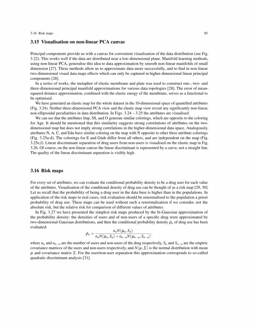
3.16 Risk maps 85
3.15 Visualisation on non-linear PCA canvas
Principal components provide us with a canvas for convenient visualisation of the data distribution (see Fig.3.22). This works well if the data are distributed near a low-dimensional plane. Manifold learning methods,using non-linear PCA, generalise this idea to data approximation by smooth non-linear manifolds of smalldimension [27]. These methods allow us to approximate data more successfully, and to find in non-lineartwo-dimensional visual data maps effects which can only be captured in higher-dimensional linear principalcomponents [28].
In a series of works, the metaphor of elastic membrane and plate was used to construct one-, two- andthree-dimensional principal manifold approximations for various data topologies [28]. The error of mean-squared distance approximation, combined with the elastic energy of the membrane, serves as a functional tobe optimised.
We have generated an elastic map for the whole dataset in the 10-dimensional space of quantified attributes(Fig. 3.24). Neither three-dimensional PCA view and the elastic map view reveal any significantly non-linear,non-ellipsoidal peculiarities in data distribution. In Figs. 3.24 – 3.25 the attributes are visualised.
We can see that the attributes Imp, SS, and O generate similar colorings, which are opposite to the coloringfor Age. It should be mentioned that this similarity suggests strong correlations of attributes on the two-dimensional map but does not imply strong correlations in the higher-dimensional data space. Analogously,attributes N, A, C, and Edu have similar coloring on the map with N opposite to other three attribute colorings(Fig. 3.25a-d). The colorings for E and Gndr differ from all others, and are independent on the map (Fig.3.25e,f). Linear discriminant separation of drug users from non-users is visualised on the elastic map in Fig.3.26. Of course, on the non-linear canvas the linear discriminant is represented by a curve, not a straight line.The quality of the linear discriminant separation is visibly high.
3.16 Risk maps
For every set of attributes, we can evaluate the conditional probability density to be a drug user for each valueof the attributes. Visualisation of the conditional density of drug use can be thought of as a risk map [29, 30].Let us recall that the probability of being a drug user in the data base is higher than in the populations. Inapplication of the risk maps to real cases, risk evaluation should be renormalised to the population a prioriprobability of drug use. These maps can be used without such a renormalisation if we consider, not theabsolute risk, but the relative risk for comparison of different values of attributes.
In Fig. 3.27 we have presented the simplest risk maps produced by the bi-Gaussian approximation ofthe probability density: the densities of users and of non-users of a specific drug were approximated bytwo-dimensional Gaussian distributions, and then the conditional probability density ρu of drug use has beenevaluated:
ρu =nuN(µu,Su)
nuN(µu,Su)+nn−uN(µn−u,Sn−u),
where nu and nn−u are the number of users and non-users of the drug respectively, Su and Sn−u are the empiriccovariance matrices of the users and non-users respectively, and N(µ,Σ) is the normal distribution with meanµ and covariance matrix Σ . For the user/non-user separation this approximation corresponds to so-calledquadratic discriminant analysis [31].

86 3 Results of data analysis
References
1. Fehrman, E., Muhammad, A.K., Mirkes, E.M., Egan, V., Gorban, A.N.: The five factor model of personality and evaluationof drug consumption risk. In: Palumbo, F., Montanari, A., Vichi, M. (eds.), Data Science, Studies in Classification, DataAnalysis, and Knowledge Organization, pp. 215–226, Springer, Cham (2017). doi:10.1007/978-3-319-55723-6 18
2. Fehrman, E., Muhammad, A.K., Mirkes, E.M., Egan, V., Gorban, A.N.: The five factor model of personality and evaluationof drug consumption risk. ArXiv preprint https://arxiv.org/abs/1506.06297 (2015). Accessed 27 Dec 2017
3. McCrae, R.R., Costa, P.T.: A contemplated revision of the NEO five-factor inventory. Personal. Individ. Differ. 36(3),587–596 (2004). doi:10.1016/s0191-8869(03)00118-1
4. Fisher, R.A.: The use of multiple measurements in taxonomic problems. Ann. Eugen. 7(2), 179–188 (1936).doi:/10.1111/j.1469-1809.1936.tb02137.x
5. Jakobwitz, S., Egan, V.: The dark triad and normal personality traits. Personal. Individ. Differ. 40(2), 331–339 (2006).doi:10.1016/j.paid.2005.07.006
6. McCrae, R.R., Costa, P.T., Terracciano, A., Parker, W.D., Mills, C.J., De Fruyt, F., Mervielde, I.: Personality trait developmentfrom 12 to 18: longitudinal, cross-sectional, and cross-cultural analyses. J. Pers. Soc. Psychol. 83(6), 1456–1468 (2002).doi:10.1037//0022-3514.83.6.1456
7. Shock, N.W., Greulich, R.C., Andres, R., Arenberg, D., Costa, P.T., Lakatta, E.G., Tobin, J.D.: Normal human aging: theBaltimore Longitudinal Study of Aging. U.S. Govermant Printing Office, Washington, DC (National Institutes of HealthPublication No. 84-2450) (1984)
8. Egan, V., Deary, I., Austin, E.: The NEO-FFI: Emerging British norms and an item-level analysis suggest N, A and C aremore reliable than O and E. Personal. Individ. Differ. 29(5), 907–920 (2000). doi:10.1016/s0191-8869(99)00242-1
9. Fridberg, D.J., Vollmer, J.M., O’Donnell, B.F., Skosnik, P.D.: Cannabis users differ from non-users on measures ofpersonality and schizotypy. Psychiatry Res. 186(1), 46–52 (2011). doi:10.1016/j.psychres.2010.07.035
10. Terracciano, A., Lockenhoff, C.E., Crum, R.M., Bienvenu, O.J., Costa, P.T.: Five-factor model personality profiles of drugusers. BMC Psychiatr. 8(1), 22 (2008). doi:10.1186/1471-244x-8-22
11. Flory, K., Lynam, D., Milich, R., Leukefeld, C., Clayton, R.: The relations among personality, symptoms of alcohol and mar-ijuana abuse, and symptoms of comorbid psychopathology: results from a community sample. Exp. Clin. Psychopharmacol.10(4), 425–434 (2002). doi:10.1037//1064-1297.10.4.425
12. Grossman, J.C., Goldstein, R., Eisenman, R.: Undergraduate marijuana and drug use as related to openness to experience.Psychiatr. Q. 48(1), 86–92 (1974). doi:10.1007/bf01574313
13. Benjamini, Y., Hochberg, Y.: Controlling the false discovery rate: a practical and powerful approach to multiple testing. J.Royal Stat. Soc. Ser. B (Methodol.) 57(1), 289–300 (1995). Available http://www.jstor.org/stable/2346101. Accessed 27Dec 2017
14. Mitchell, T.M.: Machine learning. McGraw Hill, Burr Ridge, IL (1997)15. Hastie, T., Tibshirani, R., Friedman, J.: The elements of statistical learning. Springer, New York 2009. doi:10.1007/978-0-
387-21606-516. Terentjev, P.V.: Biometrische Untersuchungen Uber Die Morpho-Logischen Merkmale Von Rana Ridibunda Pall:(Amphibia,
Salientia). Biometrika. 23(1/2) 23–51 (1931). doi:10.2307/233362917. Mitteroecker, P., Bookstein, F.: The conceptual and statistical relationship between modularity and morphological integration.
Syst. Biol. 56(5), 818–836 (2007). doi:10.1080/1063515070164802918. Berg, R.L.: The ecological significance of correlation pleiades. Evolution 14(2), 171–180 (1960). doi:10.1111/j.1558-
5646.1960.tb03076.x19. Armbruster, W.S., Di Stilio, V.S., Tuxill, J.D., Flores, T.C., Runk, J.L.: Covariance and decoupling of floral and vegetative
traits in nine Neotropical plants: a re-evaluation of Berg’s correlation-pleiades concept. Am. J. Bot. 86(1), 39–55 (1999).doi:10.2307/2656953
20. Bezdek, J.: Pattern recognition with fuzzy objective function algorithms. Plenum Press, New York (1981). doi:10.1007/978-1-4757-0450-1
21. Krishnapuram, R., Keller, J.M.: A possibilistic approach to clustering. IEEE Trans. Fuzzy Syst. 1(2), 98–110 (1993).doi:10.1109/91.227387
22. Ellis, P.D.: The Essential Guide to Effect Sizes: An Introduction to Statistical Power, Meta-Analysis and the Interpretationof Research Results. Cambridge University Press, New York (2010)
23. Blockeel, H., Struyf, J.: Efficient algorithms for decision tree cross-validation. J. Mach. Learn. Res. 3(Dec), 621–650 (2002).24. Breiman, L.: Statistical Modeling: The Two Cultures (with comments and a rejoinder by the author) Stat. Sci. 16(3), 199–231
(2001). doi:10.1214/ss/100921372625. Hand, D.J.: Classifier technology and the illusion of progress. Stat. Sci. 21(1), 1–4 (2006). doi:10.1214/088342306000000060

References 87
26. Dormann, C.F., Elith, J., Bacher, S., Buchmann, C., Carl, G., Carre, G., Marquez, J.R., Gruber, B., Lafourcade, B., Leitao,P.J., Munkemuller, T.: Collinearity: a review of methods to deal with it and a simulation study evaluating their performance.Ecography 36(1), 27–46 (2013). doi:10.1111/j.1600-0587.2012.07348.x
27. Gorban, A.N., Kegl, B., Wunsch, D.C., Zinovyev, A.Y. (eds.): Principal Manifolds for Data Visualisation and DimensionReduction. LNCSE, vol. 58, Springer, Berlin - Heidelberg - New York (2008). doi:10.1007/978-3-540-73750-6
28. Gorban, A.N., Zinovyev, A.Y.: Principal manifolds and graphs in practice: from molecular biology to dynamical systems.Int. j. neural syst. 20(03), 219–232 (2010). doi:10.1142/s0129065710002383
29. Mirkes, E.M., Alexandrakis, I., Slater, K., Tuli, R., Gorban, A.N.: Computational diagnosis and risk evaluation for caninelymphoma. Comput. Biol. Med. 53, 279–290 (2014). doi:10.1016/j.compbiomed.2014.08.006
30. Mirkes, E.M., Alexandrakis, I., Slater, K., Tuli, R., Gorban, A.N.: Computational diagnosis of canine lymphoma. J. Phys.:Conf. Ser. 490, 012135 (2014). doi:10.1088/1742-6596/490/1/012135
31. Marks, S., Dunn, O.J.: Discriminant functions when covariance matrices are unequal. J. Am. Stat. Assoc. 69(346), 555–559(1974). doi:10.1080/01621459.1974.10482992
Fig. 3.23 Elastic maps and density visualisation for the database of drug users: (a) Visualisation of the density of the data cloudon the elastic map presented in the internal coordinates, (b)-(d) Elastic map embedded in the 3-dimensional principal componentspace with various points of view. Data points are in black

88 3 Results of data analysis
Fig. 3.24 Visualisation of various functions on the elastic map (internal coordinates): (a) Age, (b) Imp, (c) SS, (d) O (Age andattributes apparently correlated with Age on the maps)

References 89
Fig. 3.25 Visualisation of various functions on the elastic map (internal coordinates): (a) N, (b) A, (c) C, (d) Edu, (e) E, (f) Gndr

90 3 Results of data analysis
(a)
Fig. 3.26 Visualisation of linear discriminant classifiers on the non-linear PCA elastic map canvas:( a) Ecstasy, (b) Heroin, (c)Benzodiazepines, (d) The group of ‘Illicit drugs’. White squares – users, black squares – non-users. Light (red) background –LDA predicts users, dark (blue) background – LDA predicts non-users
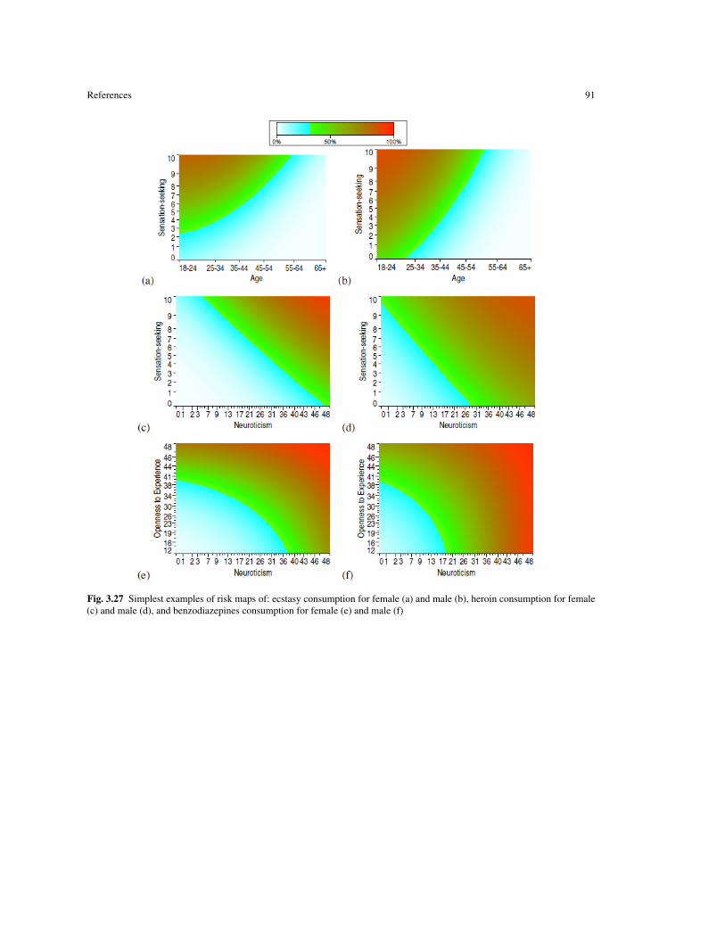
References 91
Fig. 3.27 Simplest examples of risk maps of: ecstasy consumption for female (a) and male (b), heroin consumption for female(c) and male (d), and benzodiazepines consumption for female (e) and male (f)


Summary
What have all of these data tables told us? We have asked whether or not a psychological predisposition todrug consumption exists. Now, we can formulate the answer in brief:
• There is a significant difference in the psychological profiles of drug users and non-users.• The psychological predisposition to using different drugs may be different.• Machine learning algorithms can solve the user/non-user classification problem for many drugs with im-
pressive sensitivity and specificity. Therefore, the question of predictability of the risk of drug consumptionon the basis of personality traits and simple demographic attributes is answered in the affirmative.
• Simple robust Fisher’s linear discriminants are successfully employed for this classification.• We describe the groups of drugs which have correlated use (correlation pleiades) and we can collect users
of these groups of drugs together for the purpose of analysis.• Mean profiles of users of different drugs are different. (This is explicitly proved for benzodiazepines,
ecstasy, and heroin; this is obvious from the attached tables for many more pairs of substances.)
Our study demonstrates strong correlations between personality profiles and the risk of drug use. Thisresult partially supports observations from the previous research [1–8]. For example, individuals involved inthe use of ‘heavy’ drugs like heroin and methadone are more likely to have higher scores for N, and lowerscores for A and C . In addition, they have significantly higher O, and so the typical profile is N⇑, O⇑, A⇓,and C⇓. The profile is different for recent users (within the last year) of ‘party drugs’ like ecstasy, LSD, andamyl nitrite. For them, N is not high, and the typical profile is O⇑, A⇓, and C⇓.
We have analysed, in full detail, the average differences in the groups of drug users and non-users for 18drugs (Tables 3.12, 3.13, 3.14, and 3.15). In addition to this analysis, we have achieved a much more detailedunderstanding of the relationship between personality traits, demographic data, and the use of individualdrugs or drug clusters by an individual subject.
The database we analysed contains 1,885 participants and 12 features (input attributes). These featuresinclude the five personality traits (NEO-FFI-R); impulsivity (BIS-11), sensation-seeking (ImpSS), levelof education, age, gender, country of residence, and ethnicity. The data set includes information on theconsumption of 18 central nervous system psychoactive drugs: alcohol, amphetamines, amyl nitrite, ben-zodiazepines, cannabis, chocolate, cocaine, caffeine, crack, ecstasy, heroin, ketamine, legal highs, LSD,methadone, mushrooms, nicotine, as well as VSA (output attributes).
In our analysis we used three different techniques for ranking features. After input feature ranking weexcluded ethnicity and country of residence since the dataset has not enough data for most of the ethnicities
93
94 Summary
and countries to prove the value of this information. As a result, 10 input features remained: age, Edu., N, E,O, A, C, Imp, SS, and gender. Our aim was to predict the risk of drug consumption for an individual.
All input features are ordinal or nominal. To apply data mining methods which were developed forcontinuous input features we applied the CatPCA technique to quantify the data.
We used four different definitions of drug users based on the recency of the last consumption of the drug:the decade-based, year-based, month-based and week-based user/non-user separation (Fig. 1.2).
Our findings have allowed us to draw a number of important conclusions about the associations betweenpersonality traits and drug use. All five personality factors are relevant traits to be taken into account whenassessing the risk of an individual consuming drugs.
The mean scores for the groups of users of all 18 drugs are high or neutral for N and O, and moderatelylow for A and C. The only exception is for crack usage for the week-based classification problem, which hasa moderately low (−) O score (see Table 3.15). Users of legal drugs (alcohol, chocolate, and caffeine) haveneutral A and C scores, and nicotine users have moderately low (−) C score. For LSD users in the year-basedclassification problem and for LSD and magic mushrooms users in the week-based classification problem, theA score is neutral.
The impact of the E score was found to be drug specific. For example, for the decade-based user/non-userdefinition the E score is negatively correlated with the consumption of crack, heroin, VSA, and methadone(the E score is (−) for their users). It has no predictive value for other drugs for the decade-based classification(the E score for users was (0)), whereas in the year-, month-, and week-based classification problems all threepossible values of E score were observed (see Tables 3.12, 3.13, 3.14 and 3.15).
We confirm the findings of previous researchers that higher scores for N and O, and lower scores for C andA, lead to increased risk of drug use [12]. The O score is marked by curiosity and open-mindedness (andcorrelated with intelligence), and it is therefore understandable why higher O may be sometimes be associatedwith drug use [13]. Flory et al. [4] found marijuana use to be associated with lower A and C, and higherO. These findings have been partially confirmed by our study. Our results improve the understanding of thepathways leading to drug consumption. In particular, these pathways should form paths in the correlationpleiades of drugs.
Our study has demonstrated that different attributes are important for different drugs. The detailed profilesfor users and non-users of all drugs, and groups of drugs, are collected in Tables A.1, A.2 Using these tableswe can compare, discuss, and verify almost all results and hypotheses concerning the psychological profilesof drug users. For example:
1. In the paper [5] significant differences in the NEO-PI-R mean profiles of current cocaine/heroin users andnon-users was found: for users, N⇑ and C⇓. In our table, for the month-based user definition (Table A.2),the mean profiles for cocaine users differ from non-users but the differences in A and O are also significant(p≤ 0.001): N⇑, O⇑, A⇓, and C⇓. For heroin, our table gives the result N⇑, E⇓, A⇓, and C⇓. The meanheroin user profile differs significantly from the profile for cocaine users: heroin users are significantly lessextroverted than non-users, whereas the E-score for cocaine users is found to be slightly higher than fornon-users (p = 0.129). Joining heroin users and cocaine users in one category concealed the deviations inE-score. The mean O-score of heroin users is higher than for non-users but not significantly higher (theempirical value of the O-score for heroin users is approximately the same as for cocaine users but thesignificance is different because of the different sample sizes).
2. Again in [5] and in [9] significant deviations of NEO-PI-R mean profiles for current cannabis users, fromthe means for non-users, are given as O⇑, A⇓, and C⇓. We additionally see in Table A.2 that we have N⇑.The differences in the empirical value of N-scores between cannabis users and non-users are approximatelythe same in our tables as in [5] (≈ 1), but the sample sizes are different and therefore, the statisticalsignificance differs.

Summary 95
3. In [4] a strong difference in N between cannabis users and non-users is proposed, and no significantdifferences in E and O. This result strongly contradicts our observations, as well those of other earlierworks [5, 10], which report a high difference in O and no (or more modest) difference in N.
4. Combinations of high and low scores in three NEO-FFI personality dimensions, neuroticism (N), extraver-sion (E), and conscientiousness (C), result in eight different personality types. Smoking, consumption ofalcohol and drugs, and risky sexual behaviour were studied in a sample of 683 university students in [3].Two types, E⇑, C⇓ (Impulsives, Hedonists) and N⇑, C⇓ (Insecures) were particularly inclined to engagein multiple, risky health behaviours, whereas the type with E⇓, C⇑ (Sceptics, Brooders) abstained fromrisky behaviour. Let us look at our data with the month-based user definition (Table A.2).
• Users of amphetamines, benzodiazepines, cannabis, cocaine, crack, heroin, legal highs, and nicotinebelong to the type N⇑, C⇓ (Insecures) and do not belong to the type E⇑, C⇓ (Impulsives, Hedonists).
• Users of ecstasy and LSD belong to the type E⇑, C⇓ and do not belong to the type N⇑ , C⇓.• Users of methadone belong to both types (the intersection).• It is worth mentioning that users of VSA do not belong to these types but have significant deviations in
O⇑ and in A⇓ (insufficient significance of deviation in N and C may be caused by the small samplesize with VSA).
• Users of magic mushrooms have significant deviations in O⇑ and in C⇓ but do not belong to both types(insignificance of deviation of E⇑ may be caused by the small number of magic mushroom users).
• Users of ketamine also have the profile O⇑ and in C⇓ (insignificance of deviation of N⇑ may be causedby the sample size).
• Users of amyl nitrite have profile A⇓, C⇓.• The profile with C⇑ does not exist among user profiles.
The hypothesis we make above about types of risky behaviour is partially supported by the data. Moreover,we suggest that the type E⇑, C⇓ (Impulsives, Hedonists) is more typical among ecstasy and LSD consumers,whereas the type N⇑, A⇓ is more expected among heroin users. Detailed comparison of ecstasy and heroinusers demonstrates that they are significantly different. Heroin users have higher N, and lower E and A.We also suggest that a high O-score is typical for many drug users (besides users of heroin, crack, andamyl nitrite) and therefore the O score cannot be excluded from the typology of risky behaviour. Moreover,very low A⇓ is typical for VSA users. This is especially interesting because low A is the main significantpredictor of violence in FFM and is central to the dark behaviours [11]. These comments may help in thefurther development of the typology of risky behaviour.
We tested eight types of classifiers for each drug for the decade-based user definition. Leave one outcross-validation (LOOCV) was used to evaluate sensitivity and specificity. In this study we select as thebest, the classification method which provides the maximal value of the least of sensitivity and specificity.If there is a tie on this basis, as there is in two cases, the method with maximal sum of the sensitivity andspecificity is selected as the best. There were classifiers with sensitivity and specificity greater than 70%for the decade-based user/non-user separation for all drugs except magic mushrooms, alcohol, and cocaine(Table 3.24). This accuracy was unexpectedly high for this type of problem. The poorest result was obtainedfor the prediction of alcohol consumption.
The best set of input features was defined for each drug (Table 3.24). An exhaustive search was performedto select the most effective subset of input features, and the best data mining methods to classify users andnon-users for each drug. There were 10 input features. Each of them is an important factor for risk evaluationfor the use of some drugs. However, there was no single most effective classifier using all input features. Themaximal number of attributes used in the best classifiers is six (out of 10) and the minimal number is two.

96 Summary
Table 3.24 shows the best sets of attributes for user/non-user classification for different drugs and for thedecade-based classification problem. This table, together with its analogues for pleiades of drugs and alldecade-year-month-week classification problems (Table 3.27), are important outputs of the analysis.
The decision tree (DT) for crack consumption used only two features, E and C, and provided sensitivity of80.63%, and specificity of 78.57%. The DT for VSA used age, Edu., E, A, C, and SS, and provided sensitivity83.48% and specificity 77.64% (Table 3.24).
Age was employed in the best classifiers for 14 drugs for the decade-based classification problem, and sowas a very widely used feature. Gender was used in the best methods for 10 drugs. We found some unexpectedoutcomes. For example, the fraction of females which are alcohol users is greater than the fraction of malesbut a majority of males consume caffeine (coffee).
Most of the features which are not used in the best classifiers are redundant but not uninformative. Forexample, the best classifier for ecstasy consumption used age, SS, and gender, and had sensitivity 76.17% andspecificity 77.1 6%. There is another DT which utilizes age, Edu., O, C, and SS with sensitivity 77.23% andspecificity 75.22%; a DT with inputs age, Edu., E, O, and A, with sensitivity 73.24% and specificity 78.22%,and an advanced kNN classifier with inputs age, Edu., N, E, O, C, Imp., SS, and gender, with sensitivity75.63% and specificity 75.75%. This means that for evaluating the risk of ecstasy usage all input attributesare informative but the required information can be extracted from a subset of attributes.
We have demonstrated that there are three groups of drugs with strongly correlated consumption. That is,drug usage has a ‘modular structure’. The idea of merging correlated attributes into ‘modules’ is popular inbiology. These modules are called the ‘correlation pleiades’ [14–16] (see Section ‘Pleiades of drugs’). Themodular structure contains three modules: the heroin pleiad, ecstasy pleiad, and benzodiazepines pleiad:
• The Heroin pleiad (heroinPl) includes crack, cocaine, methadone, and heroin.• The Ecstasy pleiad (ecstasyPl) includes amphetamines, cannabis, cocaine, ketamine, LSD, magic mush-
rooms, legal highs, and ecstasy.• The Benzodiazepines pleiad (benzoPl) contains methadone, amphetamines, and cocaine.
The modular structure is well represented in the correlation graph Fig 3.7. We define groups of users andnon-users for each pleiad. In most of the databases the classes of users and non-users for most of the individualdrugs are imbalanced (see Table 1.4), but merging the users of all drugs into one class ‘drug users’ does notseem to be the best solution because of physiological, psychological, and cultural differences in the usage ofdifferent drugs. We propose instead to use correlation pleiades for the analysis of drug usage as a solutionto the class imbalance problem because for all three pleiades the classes of users and non-users are betterbalanced (Table 3.25), and the consumption of different drugs from the same pleiad is correlated.
We have applied the eight methods described in the ‘Risk evaluation methods’ Section and selected thebest one for each problem for each of the pleiades. The results of the classifier selection are presented inTable 3.27 and the quality of the classification is high. The majority of the best classifiers for pleiades ofdrugs has a better accuracy than the classifiers for individual drug usage (see Tables 3.24 and 3.27). Thebest classifiers for pleiades of drugs use more input features than the best classifiers for the correspondingindividual drugs. The classification problems for pleiades of drugs are more balanced. Therefore, we expectthat the classifiers for pleiades are more robust than the classifiers for individual drugs.
The user/non-user classifiers can also be used for the formation of risk maps. Risk maps are useful toolsfor the visualisation of data and for generating hypotheses about the problem under consideration.
The limitations of the proposed analysis are obvious:
• Collection of data through the Internet with elements of the snowball technology (existing participantsrecruit future participants from amongst their acquaintances) created a biased sample.
References 97
• Our definitions of ‘substance use’ do not assume any form of dependence, and are much more inclusive andwider than the definition of substance dependence disorder [17]. Therefore, for example, the majority ofparticipants were considered as users of alcohol and caffeine. For these substances, non-users form specialcategories of interest. Similar differences in definitions are common problems. For example, standardepidemiological surveys often use data from official records with unavoidable potential biases, whereaspersonal interviews give qualitatively different information.
Now, after we finished this book, we see that our analysis is not exhaustive and we are ready to restart.Many questions should be answered. Some of them require just an extension of our analysis: for example,analyse differences between heroin and cocaine users or between cannabis and nicotine users. Some questionsare qualitatively different. For example, we considered groups of substance users but did not consider groupsof poly drug users separately. Nevertheless, these groups are not small (Figs. 3.17, 3.20) and require specialattention because of synergistic effects between different drugs. In a comparative analysis of ecstasy andheroin users we have to create classifiers for three groups: users of heroin but not ecstasy, users of ecstasy butnot heroin, and users of ecstasy and heroin. For three drugs (Fig. 3.20) we have to analyse seven groups. Suchexpansion of the data analysis will increase the research report enormously and will, perhaps, require a bookwhich is three times longer.
References
1. Sutin, A.R., Evans, M.K., Zonderman, A.B.: Personality traits and illicit substances: the moderation role of poverty. DrugAlcohol Depend. 131(3), 247–251 (2013). doi:10.1016/j.drugalcdep.2012.10.020
2. Haider, A.H., Edwin, D.H., MacKenzie, E.J., Bosse, M.J., Castillo, R.C., Travison, T.G., LEAP Study Group: The use of theNEO-five factor inventory to assess personality in trauma patients: a two-year prospective study. J. Orthop. Trauma 16(9),660–667 (2002). doi:10.1097/01.BOT.0000031328.88511.BF
3. Vollrath, M., Torgersen, S.: Who takes health risks? a probe into eight personality types. Personal. Individ. Differ. 32(7),1185–1197 (2002). doi:10.1016/s0191-8869(01)00080-0
4. Flory, K., Lynam, D., Milich, R., Leukefeld, C., Clayton, R.: The relations among personality, symptoms of alcohol and mar-ijuana abuse, and symptoms of comorbid psychopathology: results from a community sample. Exp. Clin. Psychopharmacol.10(4), 425–434 (2002). doi:10.1037//1064-1297.10.4.425
5. Terracciano, A., Lockenhoff, C.E., Crum, R.M., Bienvenu, O.J., Costa, P.T.: Five-factor model personality profiles of drugusers. BMC Psychiatr. 8(1), 22 (2008). doi:10.1186/1471-244x-8-22
6. Turiano, N.A., Whiteman, S.D., Hampson, S.E., Roberts, B.W., Mroczek, D.K.: Personality and substance use inmidlife: Conscientiousness as a moderator and the effects of trait change. J. Res. Personal. 46(3), 295–305 (2012).doi:10.1016/j.jrp.2012.02.009
7. Stewart, S.H., Devine, H.: Relations between personality and drinking motives in young adults. Personal. Individ. Differ.29(3), 495–511 (2000). doi:10.1016/s0191-8869(99)00210-x
8. Roncero, C., Daigre, C., Barral, C., Ros-Cucurull, E., Grau-Lopez, L., Rodrıguez-Cintas, L., Tarifa, N., Casas, M., Valero,S.: Neuroticism associated with cocaine-induced psychosis in cocaine-dependent patients: a cross-sectional observationalstudy. PloS one. 9(9), e106111 (2014). doi:10.1371/journal.pone.0106111
9. Fridberg, D.J., Vollmer, J.M., O’Donnell, B.F., Skosnik, P.D.: Cannabis users differ from non-users on measures ofpersonality and schizotypy. Psychiatry Res. 186(1), 46–52 (2011). doi:10.1016/j.psychres.2010.07.035
10. Grossman, J.C., Goldstein, R., Eisenman, R.: Undergraduate marijuana and drug use as related to openness to experience.Psychiatr. Q. 48(1), 86–92 (1974). doi:10.1007/bf01574313
11. Pailing, A., Boon, J., Egan, V.: Personality, the Dark Triad and violence. Pers. Individ. Differ. 67, 81–86 (2014).doi:10.1016/j.paid.2013.11.018
12. Belcher, A.M., Volkow, N.D., Moeller, F.G., Ferre, S.: Personality traits and vulnerability or resilience to substance usedisorders. Trends cogn. sci. 18(4), 211–217 (2016). doi:10.1016/j.tics.2014.01.010
13. Wilmoth, D.R.: Intelligence and past use of recreational drugs. Intelligence 40(1), 15–22 (2012).doi:10.1016/j.intell.2011.10.005

98 Summary
14. Terentjev, P.V.: Biometrische Untersuchungen Uber Die Morpho-Logischen Merkmale Von Rana Ridibunda Pall:(Amphibia,Salientia). Biometrika. 23(1/2) 23–51 (1931). doi:10.2307/2333629
15. Berg, R.L.: The ecological significance of correlation pleiades. Evolution 14(2), 171–180 (1960). doi:10.1111/j.1558-5646.1960.tb03076.x
16. Mitteroecker, P., Bookstein, F.: The conceptual and statistical relationship between modularity and morphological integration.Syst. Biol. 56(5), 818–836 (2007). doi:10.1080/10635150701648029
17. American Psychiatric Association: Diagnostic and Statistical Manual of Mental Disorders (DSM-5)https://www.psychiatry.org/psychiatrists/practice/dsm (2013) Accessed 27 Dec 2017

Discussion
These results are important as they examine the question of the relationship between drug use and personalitycomprehensively and engage in the challenge of untangling correlated personality traits (the FFM, impul-sivity, and sensation-seeking [1]), and clusters of substance misuse (the correlation pleiades). The workacknowledged the breadth of a common behaviour which may be transient and leave no impact, or maysignificantly harm an individual. We examined drug use behaviour comprehensively in terms of the manykinds of substances that may be used (from the legal and anodyne, to the deeply harmful), as well as thepossibility of behavioural over-claiming. Through inclusion of different timescales we were able to explorepersistence of use, perhaps related to trends and fashions (e.g. the greater use of LSD in the 1960s and 1970s,the rise of ecstasy in the 1980s, some people being one-off experimenters with recreational drugs, and othersusing such substances on a daily basis).
We defined substance use in terms of behaviour rather than legality, as legislation in the field is variable.Our data were gathered before legal highs emerged as a health concern [2] so we did not differentiate, forexample, synthetic cannabinoids and cathinone-based stimulants; these substances have since been widelymade illegal. We were nevertheless able to accurately classify users of these substances (reciprocally, ourdata were gathered before cannabis decriminalisation in parts of North America, but again, we were able toaccurately classify cannabis users). We included control participants who had never used these substances,those who had used them in the distant past, up to and including persons who had used the drug in the pastday, avoiding the Procrustean data-gathering and classifying methods which may prevent an accurate pictureof drug use behaviour and risk [3]. Such rich data and the complex methods used for analysis necessitated alarge and substantial sample.
The study was atheoretical regarding the morality of the behaviour, and did not medicalise or pathologiseparticipants, optimising engagement by persons with heterogeneous drug-use histories. Our study used arigorous range of data-mining methods beyond those typically used in studies examining the association ofdrug use and personality in the psychological and psychiatric literature, revealing that decision tree methodswere most commonly effective for classifying drug users. We found that high N, low A, and low C are the mostcommon personality correlates of drug use, these traits being sometimes seen, in combination, as an indicationof higher-order stability and behavioural conformity, and, inverted, are associated with externalisation ofdistress [4–6]. Deviation from this rule (N⇑, A⇓, C⇓) for some drugs is also interesting. LSD use correlateswith high O and low C (and does not correlate significantly with high N, at least, for recent LSD users). HighO is correlated with the use of many drugs. Nevertheless, there exist significant differences between profilesof different drugs. We analysed this difference in detail for benzodiazepines, ecstasy, and heroin. This may beimportant for risk assessment and treatment planning.
99

100 Discussion
Low stability is also a marker of negative urgency [7] whereby people act rashly when distressed. Ourresearch points to the importance of individuals acquiring emotional self-management skills preceding distressas a means to reduce self-medicating drug-using behaviour, and the risk to health that injudicious or chronicdrug use may cause.
In this book we have hopefully demonstrated how to use data analytic methods for investigating afascinating data set, and found some really interesting patterns in users of different drugs. Of course we havenot discovered all of the information that is hiding in the data. We invite other interested parties, be theyundergraduate, post graduate, or full time researcher, to join in with us in exploring this data to uncover moreinteresting relationships, which may help various agencies to manage the challenges associated with drug use.
References
1. Whiteside, S.P., Lynam, D.R.: The five factor model and impulsivity: Using a structural model of personality to understandimpulsivity. Pers. Individ. Differ. 30(4), 669–689 (2001). doi:10.1016/s0191-8869(00)00064-7
2. Gibbons, S.: ‘Legal Highs’–novel and emerging psychoactive drugs: a chemical overview for the toxicologist. Clin. Toxicol.50(1), 15–24 (2012). doi:10.3109/15563650.2011.645952
3. Nutt, D., King, L.A., Saulsbury, W., Blakemore, C.: Development of a rational scale to assess the harm of drugs of potentialmisuse. Lancet 369(9566), 1047–1053 (2007). doi:10.1016/s0140-6736(07)60464-4
4. Digman, J.M.: Higher-order factors of the Big Five. J. Pers. Soc. Psychol. 73(6), 1246–1256 (1997). doi:10.1037//0022-3514.73.6.1246
5. DeYoung, C.G., Peterson, J.B., Higgins, D.M.: Higher-order factors of the Big Five predict conformity: Are there neurosesof health?. Pers. Individ. Differ. 33(4), 533–552 (2002). doi:10.1016/s0191-8869(01)00171-4
6. DeYoung, C.G., Peterson, J.B., Seguin, J.R., Tremblay, R.E.: Externalizing behavior and the higher order factors of the BigFive. J. Abnorm. Psychol. 117, 947–953 (2008). doi:10.1037/a0013742
7. Settles, R.E., Fischer, S., Cyders, M.A., Combs, J.L., Gunn, R.L., Smith G.T.: Negative urgency: a personality predictorof externalizing behavior characterized by neuroticism, low conscientiousness, and disagreeableness. J. Abnorm. Psychol.121(1), 160–172 (2012). doi:10.1037/a0024948

Appendix AMain tables
A.1 Psychological profiles of drug users and non-users
Mean for groups of users and non-users. In this Appendix, we present mean T-scoresample (2.5) for groups ofusers and non-users for decade, year, month, and week based user definitions respectively. Column p-valueassesses the significance of differences of mean scores for groups of users and non-users: it is the probabilityof observing by chance the same or greater differences for mean scores if both groups have the same mean.Rows ‘#’ contain number of users and non-users for the drugs. These tables include all information about fivefactor personality profiles for various definitions of users of 18 drugs, and four groups of drugs:
• The heroin pleiad: crack, cocaine, methadone, and heroin;• The ecstasy pleiad: amphetamines, cannabis, cocaine, ketamine, LSD, magic mushrooms, legal highs, and
ecstasy;• The benzodiazepines pleiad includes methadone, amphetamines, cocaine, and benzodiazepines.• The union of these three pleiades and Volatile Substance Abuse (VSA): amphetamines, amyl nitrite,
benzodiazepines, cannabis, cocaine, crack, ecstasy, heroin, ketamine, legal highs, LSD, methadone, magicmushrooms (MMushrooms), and VSA, which we call for short ‘illicit drugs’ (with some abuse of language).
Table A.1: Mean T-scoresample (MT) and 95% CI for it for groups of users and non-users with decade and year based definitions of users
Factor Decade based Year basedUsers Non-users p-value Users Non-users p-value
MT 95% CI MT 95% CI MT 95% CI MT 95% CIAlcohol
# 1817 68 1749 136N 50.07 49.61, 50.53 48.12 45.70, 50.54 0.119 49.96 49.49, 50.43 50.55 48.87, 52.23 0.501E 50.00 49.54, 50.46 50.00 47.63, 52.36 0.997 50.12 49.64, 50.59 48.52 46.89, 50.14 0.064O 50.04 49.58, 50.50 48.86 46.51, 51.22 0.331 50.07 49.60, 50.54 49.11 47.46, 50.76 0.271A 49.91 49.45, 50.37 52.49 50.24, 54.74 0.028 49.95 49.48, 50.42 50.70 49.03, 52.37 0.392C 49.88 49.42, 50.34 53.28 51.01, 55.54 0.004 49.94 49.47, 50.41 50.73 49.03, 52.44 0.378
Imp 50.14 49.68, 50.60 46.23 44.09, 48.37 0.001 50.08 49.61, 50.55 48.96 47.31, 50.62 0.203SS 50.19 49.74, 50.65 44.81 42.57, 47.06 < 0.001 50.24 49.77, 50.71 46.91 45.24, 48.58 < 0.001
Continued on the next page
101

102 A Main tables
Table A.1. ContinuedFactor Decade based Year based
Users Non-users p-value Users Non-users p-valueMT 95% CI MT 95% CI MT 95% CI MT 95% CI
Amphetamines# 679 1206 436 1449N 51.64 50.88, 52.39 49.08 48.52, 49.64 < 0.001 52.40 51.43, 53.36 49.28 48.77, 49.78 < 0.001E 49.65 48.84, 50.47 50.20 49.66, 50.73 0.274 49.48 48.45, 50.50 50.16 49.66, 50.66 0.243O 53.05 52.34, 53.76 48.28 47.72, 48.84 < 0.001 53.83 52.92, 54.74 48.85 48.34, 49.35 < 0.001A 48.37 47.58, 49.16 50.92 50.37, 51.46 < 0.001 47.47 46.45, 48.48 50.76 50.27, 51.26 < 0.001C 46.97 46.21, 47.73 51.71 51.17, 52.25 < 0.001 45.91 44.94, 46.88 51.23 50.74, 51.72 < 0.001
Imp 53.49 52.76, 54.22 48.04 47.49, 48.58 < 0.001 54.93 54.02, 55.84 48.52 48.02, 49.01 < 0.001SS 54.76 54.12, 55.40 47.32 46.77, 47.87 < 0.001 55.79 55.01, 56.56 48.26 47.75, 48.76 < 0.001
Amyl nitrite# 370 1515 133 1752N 50.72 49.72, 51.73 49.82 49.32, 50.33 0.118 51.57 49.85, 53.29 49.88 49.41, 50.35 0.063E 50.89 49.87, 51.91 49.78 49.28, 50.29 0.055 50.25 48.44, 52.06 49.98 49.51, 50.45 0.778O 51.45 50.48, 52.42 49.65 49.14, 50.15 0.001 51.97 50.36, 53.59 49.85 49.38, 50.32 0.014A 48.65 47.62, 49.69 50.33 49.83, 50.83 0.004 46.35 44.64, 48.07 50.28 49.81, 50.74 < 0.001C 48.01 47.02, 48.99 50.49 49.98, 50.99 < 0.001 46.92 45.25, 48.60 50.23 49.77, 50.70 < 0.001
Imp 52.20 51.23, 53.18 49.46 48.96, 49.97 < 0.001 52.39 50.71, 54.08 49.82 49.35, 50.29 0.004SS 53.89 53.02, 54.77 49.05 48.54, 49.56 < 0.001 55.06 53.67, 56.44 49.62 49.15, 50.09 < 0.001
Benzodiazepines# 769 1116 535 1350N 52.77 52.06, 53.48 48.09 47.53, 48.65 < 0.001 53.69 52.84, 54.54 48.54 48.03, 49.05 < 0.001E 49.02 48.27, 49.78 50.67 50.12, 51.23 0.001 48.91 47.97, 49.85 50.43 49.92, 50.94 0.005O 52.64 51.96, 53.33 48.18 47.60, 48.76 < 0.001 53.00 52.17, 53.83 48.81 48.28, 49.34 < 0.001A 48.26 47.52, 49.01 51.20 50.64, 51.75 < 0.001 47.55 46.64, 48.46 50.97 50.46, 51.48 < 0.001C 47.62 46.90, 48.33 51.64 51.08, 52.21 < 0.001 47.07 46.19, 47.94 51.16 50.65, 51.68 < 0.001
Imp 52.53 51.82, 53.24 48.25 47.69, 48.82 < 0.001 53.35 52.52, 54.19 48.67 48.15, 49.19 < 0.001SS 52.98 52.30, 53.65 47.95 47.37, 48.52 < 0.001 54.10 53.32, 54.87 48.38 47.85, 48.90 < 0.001
Cannabis# 1265 620 999 886N 51.02 50.46, 51.58 47.92 47.19, 48.65 < 0.001 51.10 50.46, 51.74 48.76 48.14, 49.38 < 0.001E 49.69 49.12, 50.27 50.63 49.91, 51.34 0.045 49.73 49.08, 50.39 50.30 49.69, 50.91 0.217O 52.47 51.96, 52.99 44.95 44.20, 45.70 < 0.001 53.68 53.13, 54.23 45.85 45.22, 46.48 < 0.001A 48.81 48.25, 49.37 52.42 51.69, 53.15 < 0.001 48.77 48.13, 49.40 51.39 50.76, 52.02 < 0.001C 48.08 47.53, 48.63 53.92 53.22, 54.61 < 0.001 47.33 46.70, 47.95 53.02 52.42, 53.62 < 0.001
Imp 52.05 51.50, 52.61 45.81 45.13, 46.49 < 0.001 52.74 52.13, 53.36 46.91 46.30, 47.51 < 0.001SS 52.95 52.44, 53.45 43.99 43.28, 44.70 < 0.001 54.29 53.76, 54.81 45.17 44.55, 45.79 < 0.001
Chocolate# 1850 35 1840 45N 50.00 49.54, 50.45 50.21 46.31, 54.11 0.912 50.01 49.56, 50.47 49.45 46.05, 52.86 0.744E 49.99 49.53, 50.44 50.75 47.67, 53.84 0.621 49.99 49.53, 50.45 50.49 47.75, 53.24 0.716O 50.05 49.59, 50.51 47.41 44.43, 50.38 0.083 50.04 49.58, 50.50 48.27 45.59, 50.94 0.194A 50.03 49.57, 50.48 48.61 44.55, 52.67 0.486 50.02 49.56, 50.48 49.17 45.72, 52.62 0.626C 49.97 49.52, 50.43 51.55 47.83, 55.27 0.399 49.97 49.51, 50.42 51.41 47.81, 55.01 0.425
Imp 49.98 49.53, 50.44 50.81 47.30, 54.31 0.640 49.98 49.52, 50.43 50.94 47.98, 53.90 0.520SS 50.01 49.55, 50.46 49.51 45.65, 53.37 0.796 50.00 49.54, 50.45 50.06 46.84, 53.29 0.968
Continued on the next page

A.1 Psychological profiles of drug users and non-users 103
Table A.1. ContinuedFactor Decade based Year based
Users Non-users p-value Users Non-users p-valueMT 95% CI MT 95% CI MT 95% CI MT 95% CI
Cocaine# 687 1198 417 1468N 51.78 51.02, 52.54 48.98 48.42, 49.53 < 0.001 52.16 51.19, 53.13 49.39 48.88, 49.89 < 0.001E 50.27 49.49, 51.05 49.84 49.29, 50.40 0.381 50.93 49.88, 51.98 49.74 49.24, 50.23 0.044O 52.58 51.88, 53.29 48.52 47.95, 49.09 < 0.001 52.79 51.87, 53.71 49.21 48.70, 49.72 < 0.001A 47.69 46.91, 48.47 51.33 50.79, 51.86 < 0.001 46.84 45.81, 47.86 50.90 50.41, 51.39 < 0.001C 47.41 46.68, 48.14 51.48 50.93, 52.04 < 0.001 46.81 45.86, 47.76 50.91 50.40, 51.41 < 0.001
Imp 53.29 52.54, 54.03 48.12 47.57, 48.66 < 0.001 54.29 53.33, 55.25 48.78 48.29, 49.28 < 0.001SS 54.40 53.75, 55.06 47.47 46.92, 48.03 < 0.001 55.63 54.81, 56.45 48.40 47.90, 48.90 < 0.001
Caffeine# 1848 37 1824 61N 50.00 49.54, 50.45 50.06 46.57, 53.54 0.974 49.99 49.53, 50.45 50.36 47.75, 52.96 0.783E 50.07 49.61, 50.52 46.67 43.77, 49.58 0.025 50.10 49.64, 50.56 46.92 44.34, 49.50 0.018O 50.11 49.65, 50.56 44.65 41.70, 47.61 0.001 50.10 49.64, 50.56 47.07 44.45, 49.69 0.026A 49.98 49.52, 50.44 51.05 47.67, 54.42 0.529 49.96 49.50, 50.42 51.15 48.61, 53.69 0.360C 49.93 49.47, 50.39 53.56 50.75, 56.37 0.014 49.91 49.45, 50.37 52.78 50.14, 55.43 0.036
Imp 50.08 49.62, 50.53 46.10 43.15, 49.05 0.010 50.13 49.67, 50.59 46.23 43.95, 48.51 0.001SS 50.12 49.66, 50.57 44.21 41.16, 47.27 < 0.001 50.18 49.72, 50.63 44.70 42.22, 47.18 < 0.001
Crack# 191 1694 79 1806N 53.00 51.56, 54.43 49.66 49.19, 50.14 < 0.001 54.06 51.77, 56.35 49.82 49.36, 50.28 0.001E 48.74 47.28, 50.20 50.14 49.67, 50.62 0.073 49.24 47.20, 51.28 50.03 49.57, 50.50 0.455O 52.92 51.61, 54.22 49.67 49.19, 50.15 < 0.001 52.90 50.72, 55.08 49.87 49.41, 50.33 0.008A 47.00 45.44, 48.55 50.34 49.87, 50.81 < 0.001 46.65 44.18, 49.12 50.15 49.69, 50.60 0.007C 46.14 44.65, 47.63 50.44 49.97, 50.90 < 0.001 45.08 42.92, 47.25 50.22 49.76, 50.67 < 0.001
Imp 55.48 54.12, 56.85 49.38 48.91, 49.85 < 0.001 56.55 54.62, 58.48 49.71 49.25, 50.17 < 0.001SS 55.43 54.26, 56.61 49.39 48.91, 49.86 < 0.001 56.56 54.89, 58.22 49.71 49.25, 50.17 < 0.001
Ecstasy# 751 1134 517 1368N 51.24 50.52, 51.96 49.18 48.60, 49.75 < 0.001 50.71 49.82, 51.61 49.73 49.21, 50.25 0.062E 50.49 49.74, 51.24 49.68 49.11, 50.24 0.089 51.51 50.60, 52.42 49.43 48.91, 49.95 < 0.001O 53.61 52.95, 54.26 47.61 47.04, 48.18 < 0.001 54.10 53.32, 54.89 48.45 47.93, 48.97 < 0.001A 48.47 47.73, 49.20 51.01 50.45, 51.58 < 0.001 48.55 47.64, 49.45 50.55 50.03, 51.07 < 0.001C 47.22 46.52, 47.93 51.84 51.28, 52.40 < 0.001 47.02 46.17, 47.87 51.13 50.61, 51.65 < 0.001
Imp 53.04 52.35, 53.74 47.98 47.42, 48.55 < 0.001 53.74 52.91, 54.57 48.59 48.07, 49.11 < 0.001SS 54.97 54.37, 55.56 46.71 46.15, 47.27 < 0.001 55.85 55.16, 56.53 47.79 47.27, 48.31 < 0.001
Heroin# 212 1673 118 1767N 54.53 53.21, 55.85 49.43 48.95, 49.90 < 0.001 55.37 53.62, 57.12 49.64 49.18, 50.10 < 0.001E 48.38 46.90, 49.85 50.21 49.73, 50.68 0.021 47.69 45.68, 49.69 50.15 49.69, 50.62 0.019O 54.24 53.03, 55.45 49.46 48.98, 49.94 < 0.001 53.45 51.80, 55.11 49.77 49.30, 50.24 < 0.001A 45.51 43.98, 47.04 50.57 50.10, 51.03 < 0.001 44.38 42.26, 46.50 50.38 49.92, 50.83 < 0.001C 45.81 44.45, 47.17 50.53 50.06, 51.00 < 0.001 45.46 43.52, 47.39 50.30 49.84, 50.76 < 0.001
Imp 55.74 54.43, 57.06 49.27 48.80, 49.74 < 0.001 56.01 54.29, 57.74 49.60 49.14, 50.06 < 0.001SS 56.02 54.84, 57.20 49.24 48.76, 49.71 < 0.001 56.41 54.81, 58.00 49.57 49.11, 50.04 < 0.001
Continued on the next page

104 A Main tables
Table A.1. ContinuedFactor Decade based Year based
Users Non-users p-value Users Non-users p-valueMT 95% CI MT 95% CI MT 95% CI MT 95% CI
Ketamine# 350 1535 208 1677N 51.35 50.34, 52.36 49.69 49.19, 50.20 0.004 51.52 50.20, 52.84 49.81 49.33, 50.29 0.017E 50.31 49.19, 51.43 49.93 49.44, 50.42 0.542 51.02 49.48, 52.57 49.87 49.40, 50.34 0.162O 53.85 52.88, 54.82 49.12 48.62, 49.62 < 0.001 54.18 52.88, 55.48 49.48 49.01, 49.96 < 0.001A 47.78 46.64, 48.91 50.51 50.02, 51.00 < 0.001 47.90 46.42, 49.38 50.26 49.79, 50.73 0.003C 46.79 45.74, 47.85 50.73 50.24, 51.22 < 0.001 46.34 44.91, 47.76 50.45 49.98, 50.93 < 0.001
Imp 53.81 52.77, 54.85 49.13 48.64, 49.62 < 0.001 54.18 52.83, 55.53 49.48 49.01, 49.96 < 0.001SS 55.25 54.40, 56.11 48.80 48.30, 49.30 < 0.001 55.93 54.83, 57.02 49.26 48.79, 49.74 < 0.001
Legal highs# 762 1123 564 1321N 51.43 50.71, 52.16 49.03 48.45, 49.60 < 0.001 51.27 50.41, 52.12 49.46 48.93, 49.99 < 0.001E 49.66 48.89, 50.42 50.23 49.68, 50.79 0.228 50.02 49.11, 50.92 49.99 49.48, 50.51 0.966O 54.29 53.67, 54.91 47.09 46.52, 47.66 < 0.001 54.49 53.76, 55.22 48.08 47.55, 48.62 < 0.001A 48.59 47.84, 49.34 50.96 50.40, 51.51 < 0.001 48.10 47.23, 48.96 50.81 50.29, 51.34 < 0.001C 46.92 46.20, 47.65 52.09 51.54, 52.63 < 0.001 46.56 45.71, 47.41 51.47 50.95, 51.98 < 0.001
Imp 53.19 52.49, 53.89 47.83 47.28, 48.39 < 0.001 53.82 53.00, 54.63 48.37 47.85, 48.89 < 0.001SS 55.14 54.55, 55.72 46.51 45.95, 47.08 < 0.001 56.00 55.35, 56.64 47.44 46.92, 47.97 < 0.001
LSD# 557 1328 380 1505N 50.80 49.98, 51.62 49.66 49.12, 50.20 0.023 49.98 48.97, 50.99 50.00 49.50, 50.51 0.969E 50.01 49.11, 50.92 49.99 49.48, 50.51 0.971 50.72 49.63, 51.81 49.82 49.32, 50.31 0.140O 55.23 54.52, 55.93 47.81 47.28, 48.33 < 0.001 56.29 55.48, 57.10 48.41 47.91, 48.91 < 0.001A 48.40 47.53, 49.28 50.67 50.15, 51.19 < 0.001 49.05 47.98, 50.12 50.24 49.74, 50.74 0.048C 47.46 46.64, 48.29 51.06 50.53, 51.59 < 0.001 47.74 46.71, 48.77 50.57 50.07, 51.07 < 0.001
Imp 53.47 52.69, 54.25 48.54 48.01, 49.08 < 0.001 53.50 52.56, 54.43 49.12 48.61, 49.62 < 0.001SS 55.62 54.95, 56.30 47.64 47.11, 48.17 < 0.001 56.34 55.56, 57.12 48.40 47.90, 48.90 < 0.001
Methadone# 417 1468 320 1565N 53.33 52.38, 54.28 49.05 48.55, 49.56 < 0.001 53.74 52.65, 54.84 49.23 48.75, 49.72 < 0.001E 47.93 46.85, 49.01 50.59 50.10, 51.08 < 0.001 47.75 46.47, 49.03 50.46 49.99, 50.94 < 0.001O 53.78 52.87, 54.68 48.93 48.42, 49.43 < 0.001 53.81 52.76, 54.86 49.22 48.73, 49.71 < 0.001A 47.06 46.03, 48.09 50.84 50.34, 51.33 < 0.001 46.53 45.33, 47.73 50.71 50.23, 51.19 < 0.001C 46.16 45.17, 47.15 51.09 50.60, 51.58 < 0.001 46.01 44.87, 47.15 50.82 50.33, 51.30 < 0.001
Imp 53.64 52.70, 54.59 48.97 48.46, 49.47 < 0.001 53.77 52.67, 54.87 49.23 48.74, 49.72 < 0.001SS 54.45 53.56, 55.33 48.74 48.23, 49.24 < 0.001 54.73 53.73, 55.74 49.03 48.54, 49.52 < 0.001
Magic mushrooms# 694 1191 434 1451N 50.66 49.91, 51.40 49.62 49.05, 50.19 0.029 50.33 49.40, 51.26 49.90 49.38, 50.42 0.431E 50.10 49.29, 50.90 49.94 49.40, 50.49 0.758 50.71 49.66, 51.76 49.79 49.29, 50.28 0.118O 54.34 53.70, 54.99 47.47 46.91, 48.03 < 0.001 55.72 54.95, 56.48 48.29 47.78, 48.80 < 0.001A 48.52 47.75, 49.30 50.86 50.31, 51.41 < 0.001 48.51 47.48, 49.53 50.45 49.95, 50.95 0.001C 47.46 46.73, 48.20 51.48 50.92, 52.04 < 0.001 47.30 46.36, 48.24 50.81 50.30, 51.32 < 0.001
Imp 53.24 52.53, 53.95 48.11 47.55, 48.67 < 0.001 53.74 52.86, 54.63 48.88 48.37, 49.39 < 0.001SS 54.78 54.18, 55.39 47.21 46.65, 47.78 < 0.001 55.92 55.19, 56.64 48.23 47.72, 48.74 < 0.001
Continued on the next page

A.1 Psychological profiles of drug users and non-users 105
Table A.1. ContinuedFactor Decade based Year based
Users Non-users p-value Users Non-users p-valueMT 95% CI MT 95% CI MT 95% CI MT 95% CI
Nicotine# 1264 621 1060 825N 50.90 50.35, 51.45 48.16 47.40, 48.93 < 0.001 51.16 50.55, 51.76 48.52 47.85, 49.18 < 0.001E 49.91 49.35, 50.48 50.18 49.43, 50.93 0.582 49.80 49.17, 50.42 50.26 49.61, 50.91 0.309O 51.46 50.91, 52.00 47.04 46.28, 47.79 < 0.001 51.91 51.31, 52.51 47.55 46.90, 48.20 < 0.001A 49.18 48.63, 49.73 51.67 50.90, 52.44 < 0.001 49.04 48.42, 49.65 51.24 50.58, 51.90 < 0.001C 48.58 48.02, 49.14 52.89 52.17, 53.61 < 0.001 47.98 47.38, 48.57 52.60 51.95, 53.25 < 0.001
Imp 51.53 50.97, 52.09 46.89 46.17, 47.60 < 0.001 52.08 51.46, 52.69 47.33 46.71, 47.95 < 0.001SS 52.13 51.60, 52.67 45.66 44.93, 46.39 < 0.001 52.83 52.26, 53.41 46.36 45.72, 47.00 < 0.001
VSA# 230 1655 95 1790N 52.80 51.49, 54.12 49.61 49.13, 50.09 < 0.001 53.81 51.67, 55.95 49.80 49.34, 50.26 < 0.001E 48.91 47.41, 50.41 50.15 49.68, 50.62 0.122 49.55 47.32, 51.79 50.02 49.56, 50.48 0.683O 54.21 53.01, 55.40 49.42 48.93, 49.90 < 0.001 53.59 51.58, 55.60 49.81 49.35, 50.27 < 0.001A 47.28 45.90, 48.67 50.38 49.90, 50.85 < 0.001 47.48 45.35, 49.61 50.13 49.67, 50.60 0.017C 45.13 43.79, 46.47 50.68 50.21, 51.15 < 0.001 45.31 43.18, 47.44 50.25 49.79, 50.71 < 0.001
Imp 55.10 53.90, 56.30 49.29 48.81, 49.77 < 0.001 54.61 52.73, 56.49 49.76 49.29, 50.22 < 0.001SS 56.76 55.73, 57.78 49.06 48.58, 49.54 < 0.001 56.24 54.48, 57.99 49.67 49.21, 50.13 < 0.001
Heroin pleiad# 832 1053 585 1300N 51.65 50.96, 52.35 48.70 48.11, 49.28 < 0.001 52.24 51.41, 53.07 48.99 48.46, 49.52 < 0.001E 49.70 48.98, 50.41 50.24 49.66, 50.82 0.246 49.59 48.68, 50.49 50.19 49.67, 50.70 0.260O 52.75 52.11, 53.39 47.83 47.23, 48.43 < 0.001 53.02 52.25, 53.79 48.64 48.10, 49.18 < 0.001A 47.91 47.20, 48.62 51.65 51.08, 52.21 < 0.001 47.10 46.24, 47.97 51.30 50.79, 51.81 < 0.001C 47.37 46.69, 48.05 52.08 51.50, 52.65 < 0.001 46.72 45.91, 47.53 51.47 50.95, 52.00 < 0.001
Imp 52.93 52.26, 53.60 47.68 47.11, 48.26 < 0.001 53.75 52.94, 54.56 48.31 47.79, 48.83 < 0.001SS 54.00 53.39, 54.60 46.84 46.26, 47.43 < 0.001 54.87 54.16, 55.59 47.81 47.28, 48.34 < 0.001
Ecstasy pleiad# 1317 568 1089 796N 51.00 50.44, 51.55 47.68 46.94, 48.42 < 0.001 51.16 50.54, 51.78 48.41 47.77, 49.05 < 0.001E 49.69 49.13, 50.26 50.71 49.98, 51.44 0.031 49.59 48.96, 50.22 50.56 49.93, 51.20 0.033O 52.31 51.81, 52.82 44.64 43.86, 45.42 < 0.001 53.32 52.78, 53.85 45.46 44.81, 46.12 < 0.001A 48.75 48.20, 49.30 52.89 52.15, 53.64 < 0.001 48.55 47.95, 49.16 51.98 51.33, 52.63 < 0.001C 48.10 47.56, 48.64 54.40 53.70, 55.10 < 0.001 47.43 46.83, 48.02 53.52 52.91, 54.13 < 0.001
Imp 51.98 51.44, 52.52 45.41 44.72, 46.11 < 0.001 52.70 52.11, 53.29 46.31 45.69, 46.92 < 0.001SS 52.83 52.34, 53.33 43.43 42.71, 44.14 < 0.001 54.00 53.49, 54.51 44.53 43.89, 45.17 < 0.001
Benzodiazepines pleiad# 1089 796 830 1055N 51.55 50.94, 52.15 47.88 47.23, 48.54 < 0.001 52.23 51.53, 52.93 48.25 47.68, 48.82 < 0.001E 49.63 49.01, 50.25 50.51 49.85, 51.16 0.057 49.45 48.71, 50.18 50.43 49.87, 51.00 0.037O 52.28 51.70, 52.85 46.89 46.22, 47.55 < 0.001 52.86 52.20, 53.51 47.75 47.16, 48.34 < 0.001A 48.57 47.96, 49.18 51.96 51.31, 52.60 < 0.001 47.88 47.16, 48.59 51.67 51.11, 52.23 < 0.001C 47.90 47.30, 48.50 52.87 52.23, 53.51 < 0.001 47.21 46.51, 47.90 52.20 51.64, 52.76 < 0.001
Imp 52.16 51.56, 52.75 47.05 46.40, 47.69 < 0.001 53.09 52.41, 53.76 47.57 47.00, 48.14 < 0.001SS 53.00 52.44, 53.55 45.90 45.24, 46.55 < 0.001 54.13 53.52, 54.74 46.75 46.17, 47.33 < 0.001
Continued on the next page

106 A Main tables
Table A.1. ContinuedFactor Decade based Year based
Users Non-users p-value Users Non-users p-valueMT 95% CI MT 95% CI MT 95% CI MT 95% CI
Illicit drugs# 1418 467 1179 706N 51.05 50.52, 51.58 46.80 46.02, 47.58 < 0.001 51.38 50.79, 51.97 48.19 47.53, 48.84 < 0.001E 49.54 49.00, 50.09 51.39 50.62, 52.16 < 0.001 49.40 48.80, 50.01 50.93 50.27, 51.59 0.003O 51.77 51.27, 52.28 44.61 43.77, 45.45 < 0.001 52.84 52.31, 53.37 45.64 44.95, 46.33 < 0.001A 48.98 48.45, 49.51 53.11 52.31, 53.91 < 0.001 48.59 48.00, 49.17 51.99 51.34, 52.65 < 0.001C 48.37 47.84, 48.89 54.96 54.24, 55.69 < 0.001 47.61 47.04, 48.19 53.63 52.97, 54.28 < 0.001
Imp 51.64 51.12, 52.16 45.02 44.27, 45.76 < 0.001 52.46 51.89, 53.03 46.10 45.46, 46.74 < 0.001SS 52.19 51.70, 52.68 43.35 42.56, 44.13 < 0.001 53.48 52.97, 53.98 44.23 43.55, 44.90 < 0.001
Table A.2: Mean T-scoresample (MT) and 95% CI for it for groups of users and non-users with month and week based definitions of users
Factor Month based Week basedUsers Non-users p-value Users Non-users p-value
MT 95% CI MT 95% CI MT 95% CI MT 95% CIAlcohol
# 1551 334 1264 621N 49.85 49.35, 50.35 50.69 49.61, 51.78 0.167 49.82 49.28, 50.36 50.37 49.56, 51.19 0.267E 50.62 50.12, 51.11 47.14 46.11, 48.17 < 0.001 50.90 50.35, 51.44 48.17 47.38, 48.97 < 0.001O 50.22 49.73, 50.72 48.96 47.87, 50.06 0.040 50.08 49.54, 50.63 49.83 49.03, 50.62 0.602A 50.10 49.60, 50.60 49.55 48.50, 50.60 0.357 50.05 49.50, 50.60 49.89 49.09, 50.69 0.745C 50.15 49.66, 50.65 49.28 48.22, 50.35 0.146 50.19 49.64, 50.74 49.61 48.81, 50.42 0.244
Imp 50.06 49.57, 50.56 49.71 48.61, 50.82 0.571 50.19 49.64, 50.73 49.62 48.81, 50.43 0.253SS 50.34 49.85, 50.84 48.41 47.32, 49.50 0.002 50.52 49.97, 51.06 48.95 48.15, 49.75 0.001
Amphetamine# 238 1647 163 1722N 52.78 51.49, 54.07 49.60 49.12, 50.08 < 0.001 52.86 51.27, 54.45 49.73 49.26, 50.20 < 0.001E 49.07 47.63, 50.51 50.13 49.66, 50.61 0.166 48.50 46.78, 50.21 50.14 49.68, 50.61 0.069O 52.94 51.69, 54.19 49.57 49.09, 50.06 < 0.001 52.87 51.27, 54.47 49.73 49.26, 50.20 < 0.001A 46.57 45.21, 47.92 50.50 50.02, 50.97 < 0.001 46.77 45.09, 48.45 50.31 49.84, 50.77 < 0.001C 45.06 43.75, 46.37 50.71 50.24, 51.19 < 0.001 45.29 43.72, 46.85 50.45 49.98, 50.91 < 0.001
Imp 55.57 54.32, 56.83 49.19 48.72, 49.67 < 0.001 55.77 54.25, 57.29 49.45 48.99, 49.92 < 0.001SS 55.37 54.23, 56.51 49.22 48.75, 49.70 < 0.001 54.47 53.07, 55.88 49.58 49.10, 50.05 < 0.001
Amyl nitrite# 41 1844 17 1868N 49.37 46.12, 52.61 50.01 49.56, 50.47 0.691 49.64 43.99, 55.28 50.00 49.55, 50.46 0.892E 49.83 46.38, 53.28 50.00 49.55, 50.46 0.922 45.85 39.05, 52.64 50.04 49.59, 50.49 0.211O 50.40 47.06, 53.73 49.99 49.53, 50.45 0.808 49.02 43.03, 55.02 50.01 49.56, 50.46 0.732A 45.43 41.87, 49.00 50.10 49.65, 50.56 0.012 44.36 38.95, 49.77 50.05 49.60, 50.50 0.041C 47.31 44.61, 50.01 50.06 49.60, 50.52 0.049 44.81 39.74, 49.89 50.05 49.59, 50.50 0.045
Imp 54.16 50.89, 57.43 49.91 49.45, 50.36 0.013 56.76 50.49, 63.03 49.94 49.49, 50.39 0.035SS 57.33 54.76, 59.89 49.84 49.38, 50.29 < 0.001 57.30 53.19, 61.41 49.93 49.48, 50.39 0.002
Continued on the next page

A.1 Psychological profiles of drug users and non-users 107
Table A.2. ContinuedFactor Month based Week based
Users Non-users p-value Users Non-users p-valueMT 95% CI MT 95% CI MT 95% CI MT 95% CI
Benzodiazepines# 299 1586 179 1706N 55.26 54.11, 56.41 49.01 48.53, 49.48 < 0.001 56.56 55.08, 58.04 49.31 48.85, 49.77 < 0.001E 48.06 46.79, 49.33 50.37 49.89, 50.84 0.001 46.15 44.61, 47.70 50.40 49.93, 50.87 < 0.001O 52.68 51.58, 53.77 49.49 49.00, 49.99 < 0.001 52.18 50.72, 53.63 49.77 49.30, 50.25 0.002A 46.72 45.47, 47.97 50.62 50.14, 51.09 < 0.001 46.57 44.94, 48.21 50.36 49.89, 50.83 < 0.001C 46.54 45.40, 47.69 50.65 50.17, 51.14 < 0.001 46.20 44.75, 47.65 50.40 49.93, 50.87 < 0.001
Imp 54.06 52.96, 55.16 49.23 48.75, 49.72 < 0.001 53.89 52.47, 55.31 49.59 49.12, 50.06 < 0.001SS 54.36 53.34, 55.38 49.18 48.69, 49.67 < 0.001 53.62 52.28, 54.95 49.62 49.14, 50.10 < 0.001
Cannabis# 788 1097 648 1237N 50.72 49.99, 51.45 49.48 48.91, 50.06 0.009 50.62 49.82, 51.42 49.68 49.13, 50.22 0.055E 50.06 49.31, 50.80 49.96 49.40, 50.52 0.839 50.17 49.36, 50.97 49.91 49.37, 50.46 0.606O 54.34 53.74, 54.94 46.88 46.30, 47.46 < 0.001 54.70 54.05, 55.35 47.54 46.99, 48.09 < 0.001A 48.66 47.93, 49.38 50.97 50.39, 51.54 < 0.001 48.78 48.00, 49.56 50.64 50.09, 51.19 < 0.001C 47.26 46.55, 47.97 51.97 51.41, 52.52 < 0.001 47.45 46.67, 48.23 51.34 50.80, 51.88 < 0.001
Imp 53.14 52.46, 53.82 47.74 47.17, 48.31 < 0.001 53.02 52.29, 53.75 48.42 47.87, 48.97 < 0.001SS 54.82 54.25, 55.40 46.53 45.96, 47.11 < 0.001 54.87 54.22, 55.51 47.45 46.90, 48.00 < 0.001
Chocolate# 1786 99 1490 395N 49.98 49.52, 50.44 50.40 48.19, 52.60 0.714 49.95 49.44, 50.45 50.20 49.18, 51.23 0.660E 50.03 49.57, 50.49 49.43 47.38, 51.49 0.574 50.22 49.72, 50.73 49.16 48.14, 50.17 0.065O 50.05 49.58, 50.51 49.13 47.37, 50.90 0.323 49.89 49.37, 50.40 50.42 49.48, 51.36 0.327A 50.04 49.57, 50.50 49.36 47.19, 51.53 0.548 50.20 49.70, 50.70 49.23 48.19, 50.27 0.099C 49.95 49.49, 50.41 50.89 48.82, 52.97 0.380 50.13 49.62, 50.63 49.51 48.50, 50.53 0.286
Imp 49.97 49.50, 50.43 50.61 48.75, 52.46 0.508 49.93 49.43, 50.44 50.25 49.26, 51.24 0.580SS 50.02 49.55, 50.48 49.72 47.63, 51.81 0.783 49.72 49.21, 50.22 51.07 50.06, 52.08 0.019
Cocaine# 159 1726 60 1825N 52.87 51.29, 54.46 49.74 49.27, 50.21 < 0.001 53.24 50.50, 55.98 49.89 49.44, 50.35 0.019E 51.34 49.50, 53.18 49.88 49.41, 50.34 0.129 52.03 49.22, 54.84 49.93 49.48, 50.39 0.146O 52.53 51.00, 54.06 49.77 49.30, 50.24 0.001 51.40 48.83, 53.97 49.95 49.49, 50.41 0.273A 45.75 44.05, 47.46 50.39 49.93, 50.86 < 0.001 43.74 40.80, 46.68 50.21 49.75, 50.66 < 0.001C 47.23 45.72, 48.75 50.25 49.78, 50.73 < 0.001 46.72 44.32, 49.11 50.11 49.65, 50.57 0.007
Imp 54.59 53.06, 56.11 49.58 49.11, 50.05 < 0.001 54.87 52.42, 57.32 49.84 49.38, 50.30 < 0.001SS 56.48 55.10, 57.86 49.40 48.94, 49.87 < 0.001 57.38 55.14, 59.62 49.76 49.30, 50.21 < 0.001
Caffeine# 1764 121 1658 227N 50.05 49.59, 50.52 49.21 47.37, 51.05 0.379 50.07 49.59, 50.55 49.46 48.11, 50.81 0.400E 50.16 49.69, 50.63 47.68 45.94, 49.43 0.008 50.20 49.72, 50.68 48.54 47.27, 49.81 0.016O 50.12 49.65, 50.58 48.29 46.47, 50.11 0.056 50.04 49.56, 50.52 49.71 48.40, 51.03 0.645A 49.98 49.51, 50.45 50.27 48.50, 52.04 0.754 49.93 49.45, 50.41 50.48 49.15, 51.81 0.446C 49.95 49.49, 50.42 50.67 48.77, 52.56 0.473 49.95 49.47, 50.43 50.37 49.01, 51.72 0.569
Imp 50.22 49.75, 50.68 46.85 45.15, 48.55 < 0.001 50.17 49.69, 50.65 48.76 47.48, 50.04 0.043SS 50.20 49.73, 50.66 47.09 45.29, 48.90 0.001 50.11 49.63, 50.60 49.16 47.89, 50.43 0.169
Continued on the next page

108 A Main tables
Table A.2. ContinuedFactor Month based Week based
Users Non-users p-value Users Non-users p-valueMT 95% CI MT 95% CI MT 95% CI MT 95% CI
Crack# 20 1865 11 1874N 57.86 52.26, 63.45 49.92 49.46, 50.37 0.008 55.26 45.53, 64.99 49.97 49.52, 50.42 0.254E 45.97 41.31, 50.64 50.04 49.59, 50.50 0.085 46.46 38.43, 54.50 50.02 49.57, 50.47 0.348O 50.89 47.21, 54.57 49.99 49.54, 50.45 0.616 48.01 43.74, 52.28 50.01 49.56, 50.47 0.324A 42.99 36.35, 49.62 50.08 49.62, 50.53 0.038 39.62 30.12, 49.11 50.06 49.61, 50.51 0.034C 45.14 40.37, 49.91 50.05 49.60, 50.51 0.045 44.28 36.73, 51.83 50.03 49.58, 50.49 0.121
Imp 55.89 51.51, 60.27 49.94 49.48, 50.39 0.011 56.94 50.59, 63.29 49.96 49.51, 50.41 0.034SS 57.01 54.05, 59.96 49.92 49.47, 50.38 < 0.001 58.03 54.16, 61.91 49.95 49.50, 50.41 0.001
Ecstasy# 240 1645 84 1801N 49.53 48.18, 50.89 50.07 49.59, 50.55 0.465 50.28 47.99, 52.58 49.99 49.53, 50.45 0.803E 52.24 50.82, 53.65 49.67 49.20, 50.15 0.001 53.37 50.71, 56.02 49.84 49.39, 50.30 0.011O 54.41 53.23, 55.59 49.36 48.88, 49.84 < 0.001 56.15 54.15, 58.15 49.71 49.25, 50.17 < 0.001A 48.10 46.75, 49.45 50.28 49.80, 50.76 0.003 48.56 46.38, 50.75 50.07 49.61, 50.53 0.184C 47.27 45.96, 48.59 50.40 49.92, 50.88 < 0.001 46.98 44.78, 49.18 50.14 49.68, 50.60 0.006
Imp 53.43 52.19, 54.68 49.50 49.02, 49.98 < 0.001 55.71 53.49, 57.93 49.73 49.28, 50.19 < 0.001SS 55.63 54.62, 56.64 49.18 48.69, 49.66 < 0.001 56.57 54.81, 58.34 49.69 49.23, 50.15 < 0.001
Heroin# 53 1832 29 1856N 56.69 54.05, 59.34 49.81 49.35, 50.26 < 0.001 58.65 55.84, 61.47 49.86 49.41, 50.32 < 0.001E 45.58 42.06, 49.10 50.13 49.67, 50.58 0.013 44.77 39.81, 49.73 50.08 49.63, 50.53 0.038O 52.48 49.63, 55.34 49.93 49.47, 50.39 0.082 52.41 48.00, 56.81 49.96 49.51, 50.42 0.268A 42.18 39.00, 45.35 50.23 49.77, 50.68 < 0.001 41.48 38.25, 44.70 50.13 49.68, 50.59 < 0.001C 43.36 40.35, 46.37 50.19 49.74, 50.65 < 0.001 43.04 38.95, 47.12 50.11 49.66, 50.56 0.001
Imp 57.08 54.63, 59.53 49.80 49.34, 50.25 < 0.001 56.79 53.59, 59.99 49.89 49.44, 50.35 < 0.001SS 57.30 54.94, 59.66 49.79 49.33, 50.25 < 0.001 56.36 52.91, 59.81 49.90 49.45, 50.36 0.001
Ketamine# 79 1806 37 1848N 51.29 49.14, 53.45 49.94 49.48, 50.41 0.227 50.47 46.78, 54.16 49.99 49.54, 50.45 0.795E 49.62 46.74, 52.49 50.02 49.56, 50.47 0.785 47.23 42.01, 52.46 50.06 49.61, 50.50 0.282O 54.79 52.59, 56.98 49.79 49.33, 50.25 < 0.001 54.39 50.87, 57.90 49.91 49.46, 50.37 0.015A 46.90 44.15, 49.66 50.14 49.68, 50.59 0.024 44.50 40.15, 48.85 50.11 49.66, 50.56 0.013C 45.03 42.50, 47.56 50.22 49.76, 50.67 < 0.001 44.99 41.13, 48.85 50.10 49.65, 50.55 0.011
Imp 53.39 51.39, 55.38 49.85 49.39, 50.31 0.001 53.74 50.75, 56.74 49.93 49.47, 50.38 0.015SS 54.96 53.13, 56.80 49.78 49.32, 50.25 < 0.001 55.44 52.84, 58.04 49.89 49.43, 50.35 < 0.001
Legal highs# 241 1644 131 1754N 52.02 50.68, 53.36 49.70 49.23, 50.18 0.002 53.13 51.32, 54.94 49.77 49.30, 50.23 0.001E 49.10 47.59, 50.61 50.13 49.66, 50.60 0.200 47.12 45.06, 49.18 50.22 49.76, 50.67 0.004O 54.37 53.22, 55.53 49.36 48.88, 49.84 < 0.001 53.16 51.53, 54.79 49.76 49.30, 50.23 < 0.001A 46.83 45.50, 48.16 50.46 49.99, 50.94 < 0.001 46.25 44.62, 47.87 50.28 49.81, 50.75 < 0.001C 45.30 44.01, 46.60 50.69 50.21, 51.16 < 0.001 44.50 42.89, 46.11 50.41 49.95, 50.88 < 0.001
Imp 54.21 53.00, 55.41 49.38 48.90, 49.86 < 0.001 54.25 52.56, 55.94 49.68 49.22, 50.15 < 0.001SS 56.05 55.05, 57.04 49.11 48.63, 49.60 < 0.001 55.37 53.99, 56.74 49.60 49.13, 50.07 < 0.001
Continued on the next page

A.1 Psychological profiles of drug users and non-users 109
Table A.2. ContinuedFactor Month based Week based
Users Non-users p-value Users Non-users p-valueMT 95% CI MT 95% CI MT 95% CI MT 95% CI
LSD# 166 1719 69 1816N 50.55 48.97, 52.12 49.95 49.48, 50.42 0.472 50.28 47.82, 52.73 49.99 49.53, 50.45 0.820E 51.28 49.53, 53.04 49.88 49.41, 50.34 0.128 52.70 49.90, 55.51 49.90 49.44, 50.35 0.053O 57.28 56.15, 58.41 49.30 48.83, 49.77 < 0.001 57.56 55.78, 59.34 49.71 49.25, 50.17 < 0.001A 48.92 47.35, 50.48 50.10 49.63, 50.58 0.153 50.03 47.88, 52.17 50.00 49.54, 50.46 0.979C 47.10 45.59, 48.60 50.28 49.81, 50.75 < 0.001 46.98 44.90, 49.06 50.11 49.65, 50.58 0.004
Imp 53.35 51.90, 54.81 49.68 49.20, 50.15 < 0.001 52.51 50.18, 54.84 49.90 49.44, 50.36 0.032SS 56.50 55.32, 57.68 49.37 48.90, 49.84 < 0.001 56.09 54.22, 57.96 49.77 49.31, 50.23 < 0.001
Methadone# 171 1714 121 1764N 54.53 53.00, 56.06 49.55 49.08, 50.02 < 0.001 54.99 53.14, 56.84 49.66 49.20, 50.12 < 0.001E 46.86 45.08, 48.65 50.31 49.85, 50.78 < 0.001 45.27 43.11, 47.43 50.32 49.87, 50.78 < 0.001O 52.89 51.37, 54.40 49.71 49.24, 50.18 < 0.001 51.87 50.02, 53.72 49.87 49.41, 50.34 0.040A 46.18 44.50, 47.87 50.38 49.92, 50.85 < 0.001 46.00 43.84, 48.16 50.27 49.82, 50.73 < 0.001C 45.44 43.83, 47.06 50.45 49.99, 50.92 < 0.001 45.74 43.89, 47.59 50.29 49.83, 50.76 < 0.001
Imp 53.89 52.36, 55.42 49.61 49.14, 50.08 < 0.001 53.55 51.76, 55.34 49.76 49.29, 50.22 < 0.001SS 54.71 53.25, 56.17 49.53 49.06, 50.00 < 0.001 53.93 52.18, 55.67 49.73 49.27, 50.20 < 0.001
Magic mushrooms# 159 1726 44 1841N 49.91 48.41, 51.42 50.01 49.53, 50.48 0.906 49.79 46.82, 52.75 50.01 49.55, 50.46 0.884E 50.31 48.50, 52.12 49.97 49.51, 50.44 0.720 53.71 50.31, 57.12 49.91 49.46, 50.37 0.031O 56.92 55.77, 58.07 49.36 48.89, 49.83 < 0.001 57.89 55.73, 60.05 49.81 49.36, 50.27 < 0.001A 48.57 46.94, 50.19 50.13 49.66, 50.60 0.070 50.14 46.71, 53.57 50.00 49.54, 50.45 0.935C 46.85 45.25, 48.45 50.29 49.82, 50.76 < 0.001 48.03 45.33, 50.74 50.05 49.59, 50.51 0.146
Imp 53.61 52.13, 55.09 49.67 49.20, 50.14 < 0.001 55.44 52.56, 58.32 49.87 49.41, 50.33 < 0.001SS 56.18 54.94, 57.41 49.43 48.96, 49.90 < 0.001 57.95 55.75, 60.15 49.81 49.35, 50.27 < 0.001
Nicotine# 875 1010 767 1118N 51.11 50.43, 51.79 49.04 48.44, 49.64 < 0.001 51.32 50.59, 52.04 49.10 48.52, 49.67 < 0.001E 49.98 49.29, 50.66 50.02 49.42, 50.62 0.924 49.91 49.17, 50.65 50.06 49.49, 50.63 0.748O 51.86 51.19, 52.52 48.39 47.79, 48.99 < 0.001 51.57 50.85, 52.28 48.92 48.35, 49.50 < 0.001A 49.02 48.34, 49.71 50.85 50.25, 51.44 < 0.001 49.04 48.31, 49.78 50.66 50.09, 51.23 0.001C 47.69 47.03, 48.34 52.00 51.41, 52.60 < 0.001 47.69 46.99, 48.38 51.59 51.01, 52.16 < 0.001
Imp 52.48 51.80, 53.15 47.86 47.28, 48.43 < 0.001 52.56 51.84, 53.28 48.24 47.68, 48.80 < 0.001SS 52.88 52.24, 53.51 47.51 46.91, 48.10 < 0.001 52.81 52.13, 53.50 48.07 47.50, 48.64 < 0.001
VSA# 34 1851 21 1864N 51.34 47.49, 55.20 49.98 49.52, 50.43 0.479 50.92 46.02, 55.82 49.99 49.54, 50.44 0.697E 51.80 48.00, 55.60 49.97 49.51, 50.42 0.338 52.59 47.66, 57.53 49.97 49.52, 50.42 0.283O 54.65 51.65, 57.65 49.91 49.46, 50.37 0.003 56.30 53.63, 58.97 49.93 49.47, 50.38 < 0.001A 45.91 42.12, 49.71 50.08 49.62, 50.53 0.034 46.36 41.38, 51.34 50.04 49.59, 50.49 0.141C 47.22 43.63, 50.81 50.05 49.60, 50.51 0.121 49.99 45.49, 54.49 50.00 49.55, 50.45 0.995
Imp 55.93 53.25, 58.62 49.89 49.43, 50.35 < 0.001 55.21 51.37, 59.04 49.94 49.49, 50.40 0.010SS 58.61 56.27, 60.95 49.84 49.39, 50.30 < 0.001 59.05 56.49, 61.61 49.90 49.44, 50.35 < 0.001
Continued on the next page

110 A Main tables
Table A.2. ContinuedFactor Month based Week based
Users Non-users p-value Users Non-users p-valueMT 95% CI MT 95% CI MT 95% CI MT 95% CI
Heroin pleiad# 309 1576 184 1701N 53.20 52.08, 54.32 49.37 48.88, 49.86 < 0.001 54.58 53.07, 56.08 49.50 49.04, 49.97 < 0.001E 48.83 47.49, 50.18 50.23 49.76, 50.70 0.054 47.18 45.42, 48.95 50.30 49.84, 50.77 0.001O 52.60 51.51, 53.69 49.49 49.00, 49.98 < 0.001 52.13 50.69, 53.57 49.77 49.29, 50.24 0.002A 46.40 45.22, 47.59 50.71 50.22, 51.19 < 0.001 45.57 43.99, 47.16 50.48 50.01, 50.94 < 0.001C 46.69 45.54, 47.84 50.65 50.16, 51.13 < 0.001 45.57 44.13, 47.01 50.48 50.01, 50.95 < 0.001
Imp 54.24 53.12, 55.35 49.17 48.69, 49.65 < 0.001 54.25 52.81, 55.68 49.54 49.07, 50.01 < 0.001SS 55.31 54.27, 56.36 48.96 48.47, 49.44 < 0.001 55.04 53.66, 56.41 49.46 48.98, 49.93 < 0.001
Ecstasy pleiad# 921 964 792 1093N 50.98 50.30, 51.66 49.06 48.47, 49.66 < 0.001 50.94 50.22, 51.67 49.32 48.74, 49.89 0.001E 49.72 49.02, 50.41 50.27 49.69, 50.85 0.234 49.69 48.94, 50.43 50.23 49.66, 50.79 0.255O 53.86 53.29, 54.43 46.31 45.70, 46.92 < 0.001 54.07 53.46, 54.69 47.05 46.47, 47.63 < 0.001A 48.32 47.65, 48.99 51.61 51.01, 52.20 < 0.001 48.34 47.63, 49.06 51.20 50.63, 51.77 < 0.001C 47.08 46.42, 47.74 52.79 52.23, 53.35 < 0.001 47.08 46.38, 47.78 52.12 51.56, 52.67 < 0.001
Imp 53.25 52.61, 53.88 46.90 46.32, 47.48 < 0.001 53.23 52.55, 53.92 47.66 47.10, 48.22 < 0.001SS 54.58 54.03, 55.14 45.62 45.03, 46.21 < 0.001 54.64 54.05, 55.24 46.63 46.06, 47.21 < 0.001
Benzodiazepines pleiad# 528 1357 363 1522N 53.44 52.58, 54.30 48.66 48.15, 49.18 < 0.001 54.57 53.51, 55.63 48.91 48.43, 49.39 < 0.001E 48.88 47.92, 49.84 50.44 49.93, 50.94 0.005 47.72 46.57, 48.87 50.54 50.06, 51.03 < 0.001O 52.57 51.74, 53.40 49.00 48.47, 49.53 < 0.001 52.13 51.09, 53.16 49.49 48.99, 49.99 < 0.001A 47.15 46.26, 48.04 51.11 50.60, 51.62 < 0.001 46.76 45.68, 47.84 50.77 50.28, 51.26 < 0.001C 46.46 45.60, 47.32 51.38 50.87, 51.89 < 0.001 45.64 44.58, 46.69 51.04 50.55, 51.53 < 0.001
Imp 53.90 53.06, 54.75 48.48 47.97, 48.99 < 0.001 54.50 53.48, 55.52 48.93 48.44, 49.42 < 0.001SS 54.61 53.84, 55.39 48.20 47.68, 48.73 < 0.001 54.24 53.29, 55.20 48.99 48.49, 49.49 < 0.001
Illicit drugs# 996 889 862 1023N 51.33 50.67, 51.98 48.56 47.96, 49.15 < 0.001 51.41 50.70, 52.12 48.76 48.19, 49.33 < 0.001E 49.43 48.76, 50.10 51.03 50.47, 51.59 0.002 49.28 48.56, 50.01 51.13 50.59, 51.67 0.001O 53.46 52.90, 54.03 45.82 45.20, 46.45 < 0.001 53.67 53.06, 54.27 46.07 45.47, 46.66 < 0.001A 48.36 47.72, 49.00 51.48 50.87, 52.10 < 0.001 48.34 47.65, 49.03 51.19 50.60, 51.78 < 0.001C 47.22 46.58, 47.86 53.36 52.79, 53.92 < 0.001 47.09 46.41, 47.77 53.07 52.53, 53.60 < 0.001
Imp 52.97 52.36, 53.58 46.40 45.80, 46.99 < 0.001 53.08 52.42, 53.73 46.72 46.16, 47.28 < 0.001SS 54.17 53.63, 54.71 44.78 44.17, 45.40 < 0.001 54.35 53.76, 54.93 45.22 44.65, 45.79 < 0.001
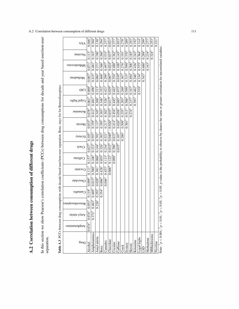
A.2 Correlation between consumption of different drugs 111A
.2C
orre
latio
nbe
twee
nco
nsum
ptio
nof
diff
eren
tdru
gs
Inth
isse
ctio
nw
esh
owPe
arso
n’s
corr
elat
ion
coef
ficie
nts
(PC
Cs)
betw
een
drug
cons
umpt
ions
for
deca
dean
dye
arba
sed
user
/non
-use
rse
para
tion.
Tabl
eA
.3PC
Cs
betw
een
drug
cons
umpt
ions
with
deca
deba
sed
user
/non
-use
rsep
arat
ion.
Ben
z.st
ays
forf
orB
enzo
diaz
epin
es.
Drug
Amphetamines
Amylnitrite
Benzodiazepines
Cannabis
Chocolate
Cocaine
Caffeine
Crack
Ecstasy
Heroin
Ketamine
Legalhighs
LSD
Methadone
MMushrooms
Nicotine
VSA
Alc
ohol
0.07
410.
0741
0.05
120.
1191
0.09
910.
1111
0.15
710.
0274
0.10
510.
0334
0.07
820.
0612
0.06
92−
0.00
740.
0711
0.11
310.
0463
Am
phet
amin
es0.
3721
0.46
310.
4691
0.01
340.
5801
0.10
610.
3231
0.59
710.
3591
0.41
210.
4811
0.49
010.
4151
0.48
110.
3431
0.30
41
Am
ylni
trite
0.22
610.
2921
0.02
840.
3811
0.06
020.
1441
0.39
210.
1371
0.34
510.
2681
0.21
310.
0841
0.27
110.
1961
0.13
01
Ben
z.0.
3541
0.00
640.
4281
0.05
520.
3261
0.38
310.
3951
0.30
310.
3481
0.35
210.
4681
0.36
610.
2601
0.29
41
Can
nabi
s0.
0463
0.45
310.
1131
0.21
610.
5211
0.21
710.
3021
0.52
610.
4211
0.29
910.
4971
0.53
310.
2371
Cho
cola
te0.
0064
0.12
210.
0324
0.04
04−
0.02
640.
0354
0.01
740.
0294
0.00
740.
0244
0.03
74−
0.02
14
Coc
aine
0.09
910.
3961
0.63
310.
4141
0.45
410.
4451
0.44
210.
3541
0.48
010.
3621
0.27
71
Caf
fein
e0.
0354
0.10
710.
0264
0.05
830.
0851
0.07
510.
0394
0.10
010.
1453
0.05
33
Cra
ck0.
2801
0.50
910.
2551
0.20
310.
2681
0.36
710.
2761
0.19
110.
2781
Ecs
tasy
0.30
110.
5111
0.58
610.
5991
0.31
510.
5991
0.37
010.
2891
Her
oin
0.27
410.
2371
0.34
710.
4941
0.30
610.
1851
0.29
31
Ket
amin
e0.
3931
0.46
210.
2461
0.43
610.
2431
0.19
21
Leg
alhi
ghs
0.51
910.
3341
0.57
510.
3641
0.31
41
LSD
0.34
310.
6801
0.28
910.
2991
Met
hado
ne0.
3431
0.23
410.
2771
MM
ushr
oom
s0.
3241
0.25
31
Nic
otin
e0.
2211
Not
e:1
p<
0.00
1,2
p<
0.01
,3p<
0.05
,4p>
0.05
.p-v
alue
isth
epr
obab
ility
toob
serv
eby
chan
ceth
esa
me
orgr
eate
rcor
rela
tion
foru
ncor
rela
ted
vari
able
s.

112 A Main tables
Tabl
eA
.4PC
Cs
betw
een
drug
cons
umpt
ions
with
year
base
dus
er/n
on-u
sers
epar
atio
n.B
enz.
stay
sfo
rfor
Ben
zodi
azep
ines
.
Drug
Amphetamines
Amylnitrite
Benzodiazepines
Cannabis
Chocolate
Cocaine
Caffeine
Crack
Ecstasy
Heroin
Ketamine
Legalhighs
LSD
Methadone
MMushrooms
Nicotine
VSA
Alc
ohol
0.04
640.
0613
0.04
820.
0783
0.07
710.
1241
0.11
110.
0581
0.10
710.
0301
0.07
240.
0931
0.08
41−
0.00
510.
0754
0.08
110.
0553
Am
phet
amin
es0.
2221
0.43
610.
4211
0.00
340.
4531
0.07
220.
1931
0.46
110.
3051
0.32
510.
4711
0.39
210.
3821
0.37
510.
3111
0.17
31
Am
ylni
trite
0.19
910.
1851
0.01
640.
2621
0.05
030.
0771
0.27
610.
1001
0.28
010.
2771
0.12
010.
0911
0.15
910.
1391
0.10
71
Ben
z.0.
3341−
0.00
940.
3651
0.06
220.
2321
0.30
410.
3181
0.26
310.
3181
0.21
210.
4641
0.27
110.
2611
0.18
31
Can
nabi
s0.
0204
0.39
210.
0742
0.16
510.
4841
0.19
910.
2771
0.51
610.
4331
0.30
110.
4701
0.51
710.
1641
Cho
cola
te0.
0084
0.08
91−
0.03
740.
0573−
0.00
340.
0004
0.02
640.
0444
0.00
640.
0194
0.00
94−
0.01
24
Coc
aine
0.06
920.
3221
0.53
510.
3581
0.37
910.
3941
0.30
210.
3141
0.34
610.
3291
0.18
71
Caf
fein
e0.
0234
0.05
930.
0234
0.02
640.
0673
0.03
240.
0274
0.05
030.
1051
0.04
24
Cra
ck0.
1561
0.35
010.
1801
0.14
710.
1391
0.26
510.
1811
0.12
610.
1451
Ecs
tasy
0.19
010.
4551
0.50
210.
5091
0.24
510.
4801
0.34
310.
1741
Her
oin
0.21
710.
1851
0.17
010.
3851
0.17
110.
1491
0.12
11
Ket
amin
e0.
3731
0.35
110.
2021
0.36
210.
2221
0.15
11
Leg
alhi
ghs
0.43
410.
3091
0.48
510.
3481
0.22
01
LSD
0.23
410.
6271
0.26
710.
1741
Met
hado
ne0.
2531
0.21
110.
1671
MM
ushr
oom
s0.
2821
0.17
41
Nic
otin
e0.
1451
Not
e:1
p<
0.00
1,2
p<
0.01
,3p<
0.05
,4p>
0.05
.p-v
alue
isth
epr
obab
ility
toob
serv
eby
chan
ceth
esa
me
orgr
eate
rcor
rela
tion
foru
ncor
rela
ted
vari
able
s.

A.3 Linear discriminants for user/non-user separation 113
A.3 Linear discriminants for user/non-user separation
Linear discriminants separate users from non-users by linear inequalities:
Θ +∑cizi > 0
for users and ≤ 0 for non-users, where Θ are the threscholds, zi are the attributes, and ci are the coefficients.Tables A.5-A.8 contain the coefficients ci of linear discriminants for user/nonuser separation in 10-dimensionalspace (7 psychological attributes, age, education, gender). The attributes in these tables are quantified andtransformed to z-scores with zero mean and unite variance (positive values of the Gndr z-score correspondsto female). The last rows of the tables include the standard deviaton of the coefficients in LOOCV. For7-dimensional space of psychological attributes taken separately (T-scores), the linear discriminants arepresented in tables A.13-A.16.
Performance of linear discriminants in user/non-user separation is evaluated by several methods (tablesA.9–A.12 for 10-dimensional data space and tables A.17–A.20 for 7-dimensional space of T-scores ofpsychological attributes). First of all, we calculated the linear discriminant using the whole sample (seetables A.5–A.8) and find all their errors. For each solution of the classification problem we have severalnumbers, P (positive), the number of samples recognised as positive, and N - negative, the number of samplesrecognised as negative. P+N is the total number of samples. P=TP+FP (True Positive plus False Positive)and N=TN+FN (True Negative plus False Negative). Sensitivity is Sn=TP/(TP+FN)×100% and Specificityis Sp=TN/(TN+FP)×100%. Accuracy is Acc=(TP+TN)/(P+N)×100%. We calculate these performanceindicators for the total sample and for the LOOCV procedure. In LOOCV the linear discriminant is calculatedfor the set of all samples excluding the example left out for testing. The test was performed for all samples withthe corresponding redefining of Sn, Sp, and Acc. In LOOCV the linear discriminants are calculated for eachtesting example. Each of these discriminants is a separate classification model. Stability of classification canbe measured by the number of examples which change their class at least once. We took the basis model forthe total sample and find how many true positive examples of this model became FN examples of a LOOCVmodel at least once. This number measured in % of TP+FP of the basic model is TP→FN. Analogously, wedefined FP→TN, TN→FP, and FN→TP. The last two numbers are measured in % of TN+FN of the basicmodel.
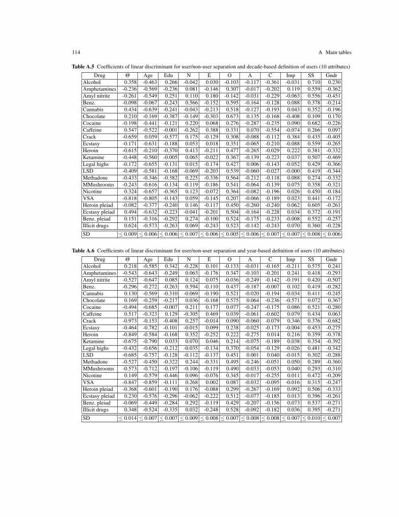
114 A Main tables
Table A.5 Coefficients of linear discriminant for user/non-user separation and decade-based definition of users (10 attributes)
Drug Θ Age Edu N E O A C Imp SS GndrAlcohol 0.358 -0.463 0.266 -0.042 0.030 -0.103 -0.117 -0.361 -0.031 0.710 0.230Amphetamines -0.236 -0.569 -0.236 0.081 -0.146 0.307 -0.017 -0.202 0.119 0.559 -0.362Amyl nitrite -0.261 -0.549 0.251 0.110 0.180 -0.142 -0.031 -0.229 -0.063 0.556 -0.451Benz. -0.098 -0.067 -0.243 0.566 -0.152 0.595 -0.164 -0.128 0.088 0.378 -0.214Cannabis 0.434 -0.639 -0.241 -0.043 -0.213 0.518 -0.127 -0.193 0.043 0.352 -0.196Chocolate 0.210 -0.169 -0.387 -0.149 -0.303 0.673 0.135 -0.168 -0.408 0.109 0.170Cocaine -0.198 -0.441 -0.121 0.220 0.068 0.276 -0.287 -0.235 0.090 0.682 -0.226Caffeine 0.547 -0.522 -0.001 -0.262 0.388 0.331 0.070 -0.554 -0.074 0.266 0.097Crack -0.659 0.059 -0.577 0.175 -0.129 0.308 -0.088 -0.112 0.384 0.435 -0.405Ecstasy -0.171 -0.631 -0.188 0.053 0.018 0.351 -0.065 -0.210 -0.088 0.559 -0.265Heroin -0.615 -0.210 -0.370 0.413 -0.211 0.477 -0.265 -0.029 0.222 0.381 -0.332Ketamine -0.448 -0.560 -0.005 0.065 -0.022 0.367 -0.139 -0.223 0.037 0.507 -0.469Legal highs -0.172 -0.655 -0.131 0.015 -0.174 0.427 0.006 -0.143 -0.052 0.429 -0.366LSD -0.409 -0.581 -0.168 -0.069 -0.203 0.539 -0.060 -0.027 -0.000 0.419 -0.344Methadone -0.433 -0.346 -0.382 0.225 -0.336 0.564 -0.212 -0.118 0.088 0.274 -0.332MMushrooms -0.243 -0.616 -0.134 -0.119 -0.186 0.541 -0.064 -0.139 0.075 0.358 -0.321Nicotine 0.324 -0.657 -0.365 0.123 -0.072 0.364 -0.082 -0.196 0.026 0.450 -0.184VSA -0.818 -0.805 -0.143 0.059 -0.145 0.207 -0.066 -0.189 0.023 0.441 -0.172Heroin pleiad -0.082 -0.377 -0.240 0.146 -0.117 0.450 -0.260 -0.240 0.062 0.605 -0.261Ecstasy pleiad 0.494 -0.632 -0.223 -0.041 -0.201 0.504 -0.164 -0.228 0.034 0.372 -0.191Benz. pleiad 0.151 -0.316 -0.292 0.274 -0.100 0.524 -0.175 -0.233 -0.008 0.552 -0.257Illicit drugs 0.624 -0.573 -0.263 0.069 -0.243 0.523 -0.142 -0.243 0.070 0.360 -0.228
SD ≤ 0.009 ≤ 0.006 ≤ 0.006 ≤ 0.007 ≤ 0.006 ≤ 0.005 ≤ 0.006 ≤ 0.007 ≤ 0.007 ≤ 0.008 ≤ 0.006
Table A.6 Coefficients of linear discriminant for user/non-user separation and year-based definition of users (10 attributes)
Drug Θ Age Edu N E O A C Imp SS GndrAlcohol 0.218 -0.585 0.342 -0.228 0.101 -0.133 -0.031 -0.165 -0.211 0.575 0.241Amphetamines -0.543 -0.643 -0.249 0.063 -0.176 0.347 -0.103 -0.201 0.241 0.418 -0.293Amyl nitrite -0.527 -0.647 0.085 0.124 0.075 -0.036 -0.249 -0.142 -0.191 0.420 -0.507Benz. -0.296 -0.272 -0.263 0.594 -0.110 0.437 -0.187 -0.007 0.102 0.419 -0.282Cannabis 0.130 -0.569 -0.310 -0.069 -0.190 0.521 -0.020 -0.194 -0.034 0.411 -0.245Chocolate 0.169 -0.259 -0.217 0.036 -0.168 0.575 0.064 -0.236 -0.571 0.072 0.367Cocaine -0.494 -0.685 -0.007 0.211 0.177 0.077 -0.247 -0.175 0.086 0.521 -0.280Caffeine 0.517 -0.323 0.129 -0.305 0.469 0.039 -0.061 -0.602 0.079 0.434 0.063Crack -0.973 -0.153 -0.408 0.257 -0.014 0.090 -0.060 -0.079 0.346 0.376 -0.682Ecstasy -0.464 -0.782 -0.101 -0.015 0.099 0.238 -0.025 -0.173 -0.004 0.453 -0.275Heroin -0.849 -0.584 -0.168 0.352 -0.252 0.222 -0.275 0.014 0.216 0.359 -0.378Ketamine -0.675 -0.790 0.033 0.070 0.046 0.214 -0.075 -0.189 0.038 0.354 -0.392Legal highs -0.432 -0.656 -0.212 -0.035 -0.134 0.370 -0.054 -0.129 -0.026 0.481 -0.342LSD -0.685 -0.757 -0.128 -0.112 -0.137 0.451 0.001 0.040 -0.015 0.302 -0.288Methadone -0.527 -0.450 -0.322 0.244 -0.331 0.495 -0.246 -0.051 0.050 0.289 -0.360MMushrooms -0.573 -0.712 -0.197 -0.106 -0.119 0.490 -0.033 -0.053 0.040 0.293 -0.310Nicotine 0.149 -0.579 -0.446 0.096 -0.076 0.345 -0.017 -0.255 0.011 0.472 -0.209VSA -0.847 -0.859 -0.111 0.268 0.002 0.087 -0.032 -0.095 -0.016 0.315 -0.247Heroin pleiad -0.368 -0.601 -0.190 0.176 -0.088 0.299 -0.267 -0.169 0.092 0.506 -0.333Ecstasy pleiad 0.230 -0.576 -0.296 -0.062 -0.222 0.512 -0.077 -0.185 0.013 0.396 -0.261Benz. pleiad -0.069 -0.449 -0.284 0.292 -0.119 0.429 -0.207 -0.156 0.073 0.537 -0.271Illicit drugs 0.348 -0.524 -0.335 0.032 -0.248 0.528 -0.092 -0.182 0.036 0.395 -0.271
SD ≤ 0.014 ≤ 0.007 ≤ 0.007 ≤ 0.009 ≤ 0.008 ≤ 0.007 ≤ 0.008 ≤ 0.008 ≤ 0.007 ≤ 0.010 ≤ 0.007

A.3 Linear discriminants for user/non-user separation 115
Table A.7 Coefficients of linear discriminant for user/non-user separation and month-based definition of users (10 attributes)
Drug Θ Age Edu N E O A C Imp SS GndrAlcohol 0.130 -0.263 0.590 0.096 0.588 -0.111 0.078 -0.083 -0.193 0.402 0.058Amphetamines -0.543 -0.643 -0.249 0.063 -0.176 0.347 -0.103 -0.201 0.241 0.418 -0.293Amyl nitrite -0.821 -0.361 -0.229 -0.223 -0.114 -0.178 -0.144 -0.018 -0.088 0.749 -0.365Benz. -0.416 -0.115 -0.243 0.711 -0.128 0.284 -0.180 0.072 0.167 0.418 -0.292Cannabis -0.122 -0.542 -0.394 -0.132 -0.166 0.547 -0.037 -0.132 0.015 0.355 -0.250Chocolate 0.132 0.138 -0.284 -0.161 0.107 0.379 -0.004 -0.440 -0.488 0.193 0.501Cocaine -0.597 -0.624 0.029 0.345 0.212 -0.007 -0.305 0.054 0.062 0.523 -0.270Caffeine 0.273 -0.019 0.369 0.261 0.637 -0.043 0.035 -0.239 0.424 0.385 0.042Crack -0.836 0.154 -0.131 0.449 -0.114 -0.075 -0.253 0.156 0.076 0.581 -0.555Ecstasy -0.633 -0.820 0.047 -0.139 0.093 0.284 -0.123 -0.165 -0.028 0.328 -0.257Heroin -1.037 -0.560 -0.371 0.181 -0.350 0.159 -0.397 0.016 0.368 0.154 -0.226Ketamine -0.793 -0.776 0.020 -0.097 -0.147 0.340 -0.098 -0.268 -0.039 0.139 -0.386Legal highs -0.693 -0.519 -0.224 -0.012 -0.190 0.409 -0.136 -0.240 0.022 0.427 -0.467LSD -0.851 -0.722 -0.173 0.006 -0.045 0.541 0.007 -0.032 -0.098 0.252 -0.284Methadone -0.551 -0.404 -0.259 0.262 -0.443 0.417 -0.270 -0.105 0.003 0.399 -0.296MMushrooms -0.764 -0.594 -0.233 -0.184 -0.236 0.604 -0.019 -0.066 0.070 0.239 -0.267Nicotine -0.019 -0.461 -0.530 0.092 0.037 0.318 0.013 -0.375 0.157 0.389 -0.283VSA -1.027 -0.785 0.003 0.081 0.059 0.174 -0.215 0.073 0.096 0.482 -0.222Heroin pleiad -0.545 -0.525 -0.187 0.301 -0.180 0.224 -0.295 0.013 0.129 0.530 -0.364Ecstasy pleiad 0.019 -0.576 -0.339 -0.133 -0.207 0.514 -0.098 -0.172 0.073 0.355 -0.241Benz. pleiad -0.346 -0.309 -0.254 0.479 -0.125 0.274 -0.215 -0.123 0.171 0.534 -0.380Illicit drugs 0.111 -0.513 -0.390 -0.034 -0.236 0.532 -0.097 -0.151 0.061 0.371 -0.267
SD ≤ 0.008 ≤ 0.006 ≤ 0.005 ≤ 0.006 ≤ 0.006 ≤ 0.006 ≤ 0.006 ≤ 0.006 ≤ 0.008 ≤ 0.008 ≤ 0.006
Table A.8 Coefficients of linear discriminant for user/non-user separation and week-based definition of users (10 attributes)
Drug Θ Age Edu N E O A C Imp SS GndrAlcohol 0.063 0.053 0.640 0.157 0.522 -0.283 0.069 -0.125 -0.105 0.412 -0.099Amphetamines -0.546 -0.441 -0.070 -0.071 -0.295 0.348 -0.207 -0.359 0.584 0.120 -0.248Amyl nitrite -0.747 0.023 0.173 -0.389 -0.351 -0.203 0.006 -0.213 0.214 0.695 -0.281Benz. -0.546 0.027 -0.331 0.680 -0.371 0.273 -0.230 0.091 0.231 0.287 -0.137Cannabis -0.240 -0.502 -0.402 -0.120 -0.172 0.594 -0.036 -0.108 -0.023 0.335 -0.253Chocolate 0.109 0.390 0.195 0.117 0.444 -0.034 0.114 -0.172 0.283 -0.461 0.513Cocaine -0.806 -0.543 0.015 0.358 0.274 -0.118 -0.299 -0.048 -0.042 0.534 -0.331Caffeine 0.131 0.484 0.200 0.335 0.637 -0.079 -0.166 -0.277 0.088 0.273 0.122Crack -1.170 0.151 -0.096 0.258 -0.068 -0.347 -0.312 0.133 0.111 0.438 -0.676Ecstasy -0.779 -0.697 0.077 -0.115 0.161 0.545 -0.093 -0.252 0.217 0.230 -0.022Heroin -1.096 -0.386 -0.077 0.467 -0.255 0.184 -0.412 0.013 0.437 -0.077 -0.400Ketamine -0.732 -0.665 0.074 -0.176 -0.223 0.380 -0.264 -0.239 -0.087 0.117 -0.423Legal highs -0.755 -0.377 -0.252 0.037 -0.302 0.300 -0.253 -0.295 -0.016 0.422 -0.531LSD -1.085 -0.679 -0.310 0.039 0.043 0.421 0.053 -0.054 -0.168 0.127 -0.462Methadone -0.606 -0.359 -0.247 0.290 -0.549 0.380 -0.242 -0.024 0.085 0.257 -0.384MMushrooms -0.657 -0.296 -0.281 -0.136 -0.046 0.705 0.036 -0.030 0.070 0.529 -0.167Nicotine -0.040 -0.252 -0.653 0.201 0.075 0.233 0.052 -0.335 0.194 0.403 -0.308VSA -1.047 -0.620 -0.042 0.076 0.016 0.270 -0.204 0.301 -0.021 0.555 -0.306Heroin pleiad -0.680 -0.390 -0.234 0.360 -0.304 0.248 -0.309 -0.119 0.136 0.431 -0.442Ecstasy pleiad -0.113 -0.524 -0.387 -0.127 -0.219 0.545 -0.093 -0.159 0.047 0.341 -0.251Benz. pleiad -0.423 -0.269 -0.305 0.504 -0.294 0.260 -0.233 -0.163 0.381 0.362 -0.265Illicit drugs -0.051 -0.471 -0.414 -0.029 -0.266 0.540 -0.080 -0.142 0.048 0.378 -0.268
SD ≤ 0.018 ≤ 0.006 ≤ 0.005 ≤ 0.005 ≤ 0.005 ≤ 0.005 ≤ 0.006 ≤ 0.005 ≤ 0.006 ≤ 0.006 ≤ 0.005

116 A Main tables
Table A.9 Performance and stability of linear discriminant for decade-based definition of users (10 attributes).
Total sample LOOCV Stability indicatorsDrug Sn Sp Acc Sn Sp Acc TP→FN FN→TP FP→TN TN→FPAlcohol 65.1 67.6 65.2 64.9 57.4 64.6 5.8 8.5 11.8 7.4Amphetamines 72.0 71.9 71.9 71.1 71.5 71.4 1.2 0.9 0.7 0.5Amyl nitrite 63.8 63.6 63.6 62.2 63.0 62.9 2.4 1.6 1.3 1.8Benz. 67.4 67.5 67.4 66.8 67.1 67.0 0.4 0.4 0.6 1.3Cannabis 78.1 78.2 78.1 77.9 77.6 77.8 0.4 0.6 0.8 1.0Chocolate 57.9 57.1 57.9 57.5 37.1 57.1 11.2 14.3 14.1 28.6Cocaine 67.7 67.6 67.6 67.0 67.3 67.2 0.9 0.6 0.5 1.0Caffeine 68.7 70.3 68.8 68.6 62.2 68.5 5.5 8.8 8.1 13.5Crack 69.6 69.1 69.1 65.4 68.9 68.5 5.2 2.1 1.7 1.7Ecstasy 74.4 74.7 74.6 74.2 74.3 74.2 0.3 0.7 0.5 0.4Heroin 70.8 69.9 70.0 68.4 69.8 69.7 2.8 6.1 1.3 2.2Ketamine 68.0 67.8 67.8 66.6 67.5 67.3 1.4 1.4 0.5 1.4Legal highs 79.0 79.2 79.1 78.9 78.9 78.9 0.1 0.8 0.3 0.4LSD 76.8 76.7 76.8 76.5 76.7 76.6 0.5 0.7 0.5 0.7Methadone 70.5 70.8 70.7 69.3 70.2 70.0 1.2 0.7 1.4 0.5MMushrooms 75.6 75.7 75.6 75.1 75.3 75.2 0.9 0.1 0.7 0.5Nicotine 70.1 70.4 70.2 69.7 69.1 69.5 0.8 0.9 1.6 1.1VSA 74.8 74.8 74.8 74.3 74.7 74.5 2.2 2.2 0.7 1.6Heroin pleiad 69.6 70.1 69.9 69.1 69.4 69.3 0.5 0.7 0.9 0.4Ecstasy pleiad 78.6 78.7 78.6 78.6 78.2 78.5 0.5 0.8 0.4 0.4Benz. pleiad 70.7 70.7 70.7 70.2 69.8 70.0 0.9 0.8 0.9 0.8Illicit drugs 77.9 78.2 78.1 77.5 77.8 77.7 0.4 0.6 0.7 0.9
Table A.10 Performance and stability of linear discriminant for year-based definition of users (10 attributes).
Total sample LOOCV Stability indicatorsDrug Sn Sp Acc Sn Sp Acc TP→FN FN→TP FP→TN TN→FPAlcohol 63.1 63.2 63.1 62.7 58.1 62.4 3.3 4.6 5.9 4.4Amphetamines 72.5 72.7 72.7 71.6 72.4 72.2 0.9 0.5 0.9 0.9Amyl nitrite 69.2 68.6 68.6 62.4 68.3 67.9 4.5 2.3 2.7 2.6Benz. 69.7 69.4 69.5 68.2 69.3 69.0 1.9 0.6 0.5 0.7Cannabis 79.3 79.3 79.3 78.9 79.0 78.9 0.7 0.8 0.3 0.2Chocolate 58.1 60.0 58.1 57.4 37.8 57.0 13.6 16.1 17.8 13.3Cocaine 71.0 71.5 71.4 69.8 71.1 70.8 1.0 0.2 1.0 1.2Caffeine 68.0 67.2 68.0 67.7 54.1 67.2 8.9 7.3 11.5 6.6Crack 73.4 73.9 73.9 69.6 73.6 73.4 1.3 2.5 3.4 3.7Ecstasy 75.4 75.7 75.6 75.0 75.6 75.4 0.2 0.6 0.8 0.3Heroin 73.7 73.7 73.7 70.3 73.6 73.4 2.5 2.5 2.1 2.3Ketamine 71.6 71.6 71.6 68.8 71.4 71.1 2.9 1.9 2.1 1.9Legal highs 77.7 77.7 77.7 77.0 77.4 77.3 0.9 0.4 0.5 0.5LSD 80.0 80.0 80.0 79.2 79.9 79.7 0.5 0.5 0.3 0.9Methadone 70.6 70.6 70.6 69.7 70.4 70.3 0.9 0.9 0.7 1.7MMushrooms 77.9 77.9 77.9 77.4 77.7 77.7 0.5 0.2 0.2 0.6Nicotine 70.4 70.4 70.4 70.1 70.2 70.1 0.3 0.8 0.4 0.4VSA 72.6 72.7 72.7 71.6 72.5 72.4 2.1 2.1 1.7 3.9Heroin pleiad 71.5 72.0 71.8 71.3 71.7 71.6 0.3 0.7 0.8 1.0Ecstasy pleiad 80.2 80.3 80.2 80.0 80.0 80.0 0.1 0.6 0.3 0.5Benz. pleiad 73.0 72.7 72.8 72.4 72.3 72.4 0.6 0.4 0.5 0.4Illicit drugs 80.2 79.6 79.8 79.5 79.4 79.4 1.0 0.4 0.4 0.3

A.3 Linear discriminants for user/non-user separation 117
Table A.11 Performance and stability of linear discriminant for month-based definition of users (10 attributes).
Total sample LOOCV Stability indicatorsDrug Sn Sp Acc Sn Sp Acc TP→FN FN→TP FP→TN TN→FPAlcohol 60.9 61.1 60.9 60.4 58.4 60.1 2.3 2.6 3.0 2.4Amphetamines 68.9 68.1 68.2 65.5 68.0 67.7 2.9 3.4 1.2 2.0Amyl nitrite 70.7 75.3 75.2 63.4 75.1 74.9 2.4 2.4 8.5 5.2Benz. 68.9 68.7 68.8 68.2 68.5 68.5 1.3 1.3 1.1 2.0Cannabis 78.6 78.3 78.4 77.7 77.9 77.8 1.1 0.0 0.6 0.9Chocolate 57.9 56.6 57.8 57.2 48.5 56.7 9.7 8.0 9.1 8.1Cocaine 69.8 70.0 70.0 67.3 69.9 69.7 3.1 2.5 2.3 2.7Caffeine 60.8 60.3 60.7 60.5 54.5 60.2 7.3 5.2 6.6 5.8Crack 80.0 75.3 75.4 65.0 75.2 75.1 15.0 15.0 4.8 11.6Ecstasy 72.5 72.4 72.4 71.3 72.3 72.1 1.7 1.3 1.2 1.2Heroin 79.2 77.6 77.7 69.8 77.5 77.2 9.4 7.5 3.2 3.8Ketamine 72.2 73.3 73.2 64.6 73.1 72.8 3.8 1.3 3.4 2.7Legal highs 72.6 72.5 72.5 71.4 72.4 72.3 1.2 1.7 0.9 1.2LSD 76.5 76.4 76.4 74.7 76.3 76.2 1.2 1.2 1.0 1.9Methadone 68.4 68.1 68.2 66.7 67.7 67.6 1.8 3.5 1.6 2.6MMushrooms 75.5 74.3 74.4 73.6 74.3 74.2 2.5 2.5 0.9 2.0Nicotine 66.4 66.2 66.3 65.8 66.0 65.9 1.1 0.7 0.3 0.7VSA 76.5 75.6 75.6 58.8 75.6 75.3 5.9 5.9 2.9 6.1Heroin pleiad 69.3 69.4 69.4 68.0 69.2 69.0 1.6 1.3 1.5 0.9Ecstasy pleiad 79.4 79.6 79.5 79.2 79.1 79.2 0.5 0.5 0.7 0.7Benz. pleiad 70.5 70.3 70.3 70.1 69.9 70.0 0.4 0.8 0.7 1.0Illicit drugs 78.9 78.8 78.8 78.4 78.5 78.5 0.4 0.3 0.5 0.4
Table A.12 Performance and stability of linear discriminant for week-based definition of users (10 attributes).
Total sample LOOCV Stability indicatorsDrug Sn Sp Acc Sn Sp Acc TP→FN FN→TP FP→TN TN→FPAlcohol 60.4 59.9 60.3 59.3 58.9 59.2 2.0 0.9 1.0 1.3Amphetamines 66.9 66.7 66.7 62.0 66.5 66.1 4.3 2.5 3.0 2.8Amyl nitrite 70.6 77.6 77.5 52.9 77.4 77.1 0.0 5.9 14.7 11.8Benz. 70.4 70.1 70.1 67.0 69.8 69.5 3.4 1.7 2.1 2.7Cannabis 75.9 75.9 75.9 75.3 75.5 75.4 0.9 0.0 0.5 0.5Chocolate 57.8 57.7 57.8 57.2 54.4 56.6 3.6 2.5 3.3 1.3Cocaine 75.0 75.1 75.1 61.7 75.1 74.6 8.3 6.7 4.1 4.4Caffeine 59.5 58.1 59.4 58.5 52.0 57.7 5.8 2.8 6.2 5.3Crack 90.9 85.9 85.9 54.5 85.8 85.6 27.3 9.1 4.1 7.7Ecstasy 72.6 71.5 71.5 67.9 71.4 71.2 3.6 8.3 2.4 5.3Heroin 79.3 80.1 80.1 65.5 80.0 79.8 6.9 6.9 4.6 4.8Ketamine 73.0 71.9 71.9 62.2 71.6 71.5 8.1 8.1 3.5 6.5Legal highs 70.2 71.0 71.0 66.4 70.9 70.6 3.8 5.3 2.5 1.9LSD 81.2 80.6 80.6 76.8 80.3 80.2 4.3 2.9 1.5 2.2Methadone 70.2 69.4 69.5 65.3 69.3 69.1 3.3 4.1 2.6 3.2MMushrooms 70.5 68.7 68.7 61.4 68.4 68.2 6.8 9.1 4.4 7.9Nicotine 63.9 63.8 63.8 63.5 63.5 63.5 0.5 0.8 0.3 0.6VSA 81.0 78.7 78.7 61.9 78.6 78.4 4.8 0.0 5.2 7.7Heroin pleiad 70.7 70.3 70.3 65.8 69.8 69.4 4.9 1.6 2.1 1.6Ecstasy pleiad 77.3 77.3 77.3 76.6 77.0 76.9 0.6 0.3 0.6 0.8Benz. pleiad 68.3 68.5 68.4 66.9 68.3 68.0 1.1 1.1 1.2 0.9Illicit drugs 77.2 77.1 77.2 76.8 76.7 76.8 0.7 0.8 0.7 0.5

118 A Main tables
Table A.13 Coefficients of linear discriminant for user/non-user separation and decade-based definition of users (7 attributes)
Drug Θ N E O A C Imp SSAlcohol -22.282 0.124 0.149 -0.068 -0.102 -0.460 0.056 0.856Amphetamines -36.596 0.040 -0.197 0.363 -0.063 -0.343 0.040 0.840Amyl nitrite -29.255 0.083 0.177 -0.023 -0.104 -0.308 -0.195 0.904Benz. -56.705 0.532 -0.211 0.597 -0.205 -0.186 0.105 0.478Cannabis -22.278 -0.004 -0.242 0.571 -0.143 -0.357 -0.014 0.684Chocolate 6.158 -0.133 -0.369 0.603 0.271 -0.308 -0.467 0.309Cocaine -43.257 0.203 0.037 0.303 -0.288 -0.293 0.024 0.834Caffeine -9.371 -0.121 0.479 0.313 0.026 -0.682 -0.139 0.416Crack -48.494 0.145 -0.293 0.326 -0.202 -0.243 0.415 0.718Ecstasy -35.896 0.045 -0.017 0.407 -0.085 -0.342 -0.156 0.827Heroin -55.851 0.381 -0.283 0.526 -0.322 -0.124 0.249 0.563Ketamine -34.711 -0.003 -0.094 0.478 -0.197 -0.333 -0.024 0.782Legal highs -30.803 -0.017 -0.227 0.532 -0.040 -0.303 -0.118 0.747LSD -34.972 -0.108 -0.258 0.632 -0.103 -0.162 -0.068 0.694Methadone -27.409 0.208 -0.416 0.620 -0.262 -0.253 0.058 0.513MMushrooms -29.576 -0.147 -0.239 0.631 -0.106 -0.265 0.002 0.665Nicotine -38.644 0.171 -0.092 0.397 -0.093 -0.393 0.005 0.801VSA -34.395 0.071 -0.209 0.326 -0.060 -0.392 0.012 0.829Heroin pleiad -30.383 0.113 -0.149 0.441 -0.270 -0.331 0.007 0.767Ecstasy pleiad -17.510 -0.002 -0.222 0.542 -0.180 -0.385 -0.028 0.689Benz. pleiad -35.808 0.232 -0.136 0.492 -0.201 -0.347 -0.042 0.723Illicit drugs -18.501 0.096 -0.272 0.537 -0.169 -0.409 0.014 0.657
SD ≤ 0.970 ≤ 0.008 ≤ 0.008 ≤ 0.007 ≤ 0.007 ≤ 0.008 ≤ 0.008 ≤ 0.009
Table A.14 Coefficients of linear discriminant for user/non-user separation and year-based definition of users (7 attributes)
Drug Θ N E O A C Imp SSAlcohol -16.181 -0.136 0.270 -0.082 -0.024 -0.236 -0.314 0.865Amphetamines -39.624 0.061 -0.213 0.424 -0.136 -0.365 0.166 0.769Amyl nitrite -5.472 0.060 0.023 0.157 -0.388 -0.292 -0.319 0.796Benz. -64.199 0.566 -0.171 0.456 -0.220 -0.112 0.089 0.611Cannabis -24.008 -0.064 -0.230 0.555 -0.040 -0.354 -0.093 0.706Chocolate 0.709 0.114 -0.159 0.582 0.264 -0.380 -0.606 0.203Cocaine -46.414 0.224 0.152 0.187 -0.299 -0.292 0.030 0.846Caffeine -8.114 -0.222 0.503 0.076 -0.063 -0.636 0.052 0.530Crack -52.425 0.244 -0.153 0.140 -0.219 -0.282 0.399 0.782Ecstasy -42.579 -0.019 0.078 0.373 -0.045 -0.356 -0.096 0.846Heroin -44.733 0.361 -0.327 0.368 -0.397 -0.108 0.218 0.641Ketamine -42.342 0.056 -0.003 0.417 -0.143 -0.363 -0.047 0.818Legal highs -30.027 -0.062 -0.181 0.460 -0.091 -0.300 -0.098 0.803LSD -40.183 -0.141 -0.220 0.650 -0.039 -0.118 -0.115 0.693Methadone -28.093 0.234 -0.417 0.575 -0.296 -0.206 0.024 0.556MMushrooms -36.864 -0.142 -0.182 0.669 -0.093 -0.215 -0.053 0.664Nicotine -35.594 0.122 -0.126 0.376 -0.036 -0.441 0.019 0.795VSA -55.631 0.382 0.009 0.213 -0.038 -0.379 -0.014 0.815Heroin pleiad -32.917 0.154 -0.147 0.385 -0.310 -0.312 0.044 0.782Ecstasy pleiad -20.439 -0.059 -0.264 0.548 -0.102 -0.354 -0.045 0.699Benz. pleiad -41.126 0.256 -0.164 0.438 -0.230 -0.287 0.018 0.761Illicit drugs -22.701 0.033 -0.295 0.549 -0.125 -0.351 -0.012 0.686
SD ≤ 1.250 ≤ 0.011 ≤ 0.011 ≤ 0.009 ≤ 0.009 ≤ 0.009 ≤ 0.008 ≤ 0.012

A.3 Linear discriminants for user/non-user separation 119
Table A.15 Coefficients of linear discriminant for user/non-user separation and month-based definition of users (7 attributes)
Drug Θ N E O A C Imp SSAlcohol -63.256 0.190 0.823 0.002 0.087 -0.005 -0.268 0.456Amphetamines -24.230 0.011 -0.223 0.361 -0.254 -0.499 0.375 0.605Amyl nitrite -6.284 -0.243 -0.183 -0.082 -0.187 -0.092 -0.117 0.918Benz. -69.623 0.702 -0.189 0.286 -0.215 0.006 0.148 0.568Cannabis -25.637 -0.145 -0.215 0.606 -0.069 -0.322 -0.051 0.674Chocolate 19.518 -0.121 0.254 0.308 0.168 -0.595 -0.621 0.240Cocaine -57.737 0.366 0.148 0.082 -0.370 -0.014 -0.001 0.837Caffeine -91.137 0.351 0.687 0.026 0.052 -0.080 0.567 0.271Crack -46.531 0.459 -0.220 -0.077 -0.357 0.096 0.066 0.771Ecstasy -27.572 -0.169 0.101 0.462 -0.191 -0.354 -0.139 0.752Heroin -30.020 0.302 -0.409 0.232 -0.499 -0.107 0.345 0.555Ketamine -6.182 -0.169 -0.210 0.643 -0.232 -0.464 -0.044 0.493Legal highs -17.306 -0.067 -0.240 0.474 -0.201 -0.388 -0.053 0.721LSD -47.031 -0.012 -0.097 0.762 -0.023 -0.225 -0.155 0.578Methadone -17.825 0.260 -0.501 0.436 -0.286 -0.238 -0.004 0.594MMushrooms -29.897 -0.229 -0.273 0.762 -0.037 -0.217 -0.019 0.494Nicotine -34.684 0.072 -0.032 0.342 -0.022 -0.590 0.204 0.698VSA -70.559 0.137 0.068 0.230 -0.208 -0.073 0.182 0.918Heroin pleiad -41.444 0.277 -0.272 0.284 -0.346 -0.105 0.113 0.791Ecstasy pleiad -19.318 -0.141 -0.257 0.573 -0.125 -0.359 0.014 0.664Benz. pleiad -47.877 0.416 -0.199 0.300 -0.258 -0.246 0.128 0.745Illicit drugs -21.767 -0.051 -0.295 0.567 -0.129 -0.344 0.009 0.674
SD ≤ 1.041 ≤ 0.009 ≤ 0.009 ≤ 0.009 ≤ 0.008 ≤ 0.007 ≤ 0.007 ≤ 0.010
Table A.16 Coefficients of linear discriminant for user/non-user separation and week-based definition of users (7 attributes)
Drug Θ N E O A C Imp SSAlcohol -52.758 0.202 0.791 -0.273 0.041 -0.002 -0.176 0.476Amphetamines -17.930 -0.054 -0.311 0.402 -0.237 -0.472 0.577 0.356Amyl nitrite 5.116 -0.466 -0.348 -0.188 -0.084 -0.186 0.249 0.723Benz. -51.825 0.707 -0.438 0.240 -0.229 0.052 0.224 0.382Cannabis -28.488 -0.136 -0.215 0.658 -0.074 -0.282 -0.079 0.641Chocolate -22.538 0.221 0.565 -0.149 0.195 0.020 0.302 -0.693Cocaine -42.900 0.347 0.198 -0.011 -0.407 -0.090 -0.103 0.810Caffeine -53.485 0.422 0.821 -0.118 -0.135 -0.146 0.301 -0.061Crack -22.095 0.304 -0.279 -0.282 -0.463 0.148 0.119 0.707Ecstasy -60.127 -0.095 0.168 0.695 -0.128 -0.355 0.242 0.528Heroin -37.099 0.548 -0.325 0.265 -0.547 -0.069 0.389 0.261Ketamine 1.992 -0.284 -0.395 0.574 -0.307 -0.228 -0.030 0.535Legal highs 0.347 -0.015 -0.352 0.406 -0.315 -0.454 -0.022 0.636LSD -35.647 0.001 0.054 0.716 0.008 -0.371 -0.309 0.501Methadone -14.932 0.317 -0.636 0.331 -0.310 -0.106 0.084 0.521MMushrooms -66.891 -0.143 -0.071 0.715 0.073 -0.114 0.059 0.665Nicotine -42.383 0.175 -0.013 0.222 0.012 -0.574 0.284 0.714VSA -75.762 0.043 -0.068 0.419 -0.191 0.250 0.056 0.846Heroin pleiad -25.458 0.341 -0.397 0.242 -0.379 -0.205 0.116 0.684Ecstasy pleiad -19.877 -0.146 -0.272 0.603 -0.124 -0.338 -0.004 0.642Benz. pleiad -43.258 0.498 -0.349 0.260 -0.250 -0.274 0.343 0.554Illicit drugs -22.772 -0.055 -0.329 0.575 -0.113 -0.322 0.004 0.665
SD ≤ 0.707 ≤ 0.006 ≤ 0.006 ≤ 0.006 ≤ 0.007 ≤ 0.007 ≤ 0.009 ≤ 0.007

120 A Main tables
Table A.17 Performance and stability of linear discriminant for decade-based definition of users (7 attributes).
Total sample LOOCV Stability indicatorsDrug Sn Sp Acc Sn Sp Acc TP→FN FN→TP FP→TN TN→FPAlcohol 67.1 64.7 67.0 66.9 55.9 66.5 7.6 4.7 11.8 4.4Amphetamines 69.1 69.3 69.2 68.5 68.7 68.6 0.7 1.0 1.1 1.2Amyl nitrite 61.9 61.8 61.9 61.1 61.7 61.5 1.6 2.4 0.9 2.0Benz. 67.6 67.3 67.4 67.0 66.8 66.9 0.8 0.7 0.8 0.9Cannabis 75.0 75.2 75.1 74.9 74.4 74.7 0.5 0.5 0.8 0.6Chocolate 56.7 54.3 56.7 56.4 42.9 56.2 11.4 13.1 5.7 20.0Cocaine 66.4 66.5 66.5 66.1 66.2 66.2 0.4 0.6 0.7 0.7Caffeine 69.9 70.3 69.9 69.7 56.8 69.4 6.5 7.5 10.8 8.1Crack 66.0 65.9 65.9 62.8 65.6 65.3 4.7 1.6 2.1 2.6Ecstasy 71.6 71.6 71.6 71.4 71.4 71.4 0.5 0.8 0.4 0.7Heroin 70.3 70.8 70.7 68.4 70.6 70.3 1.9 1.4 2.1 1.6Ketamine 66.9 66.8 66.8 65.1 66.6 66.4 2.3 2.0 1.2 1.1Legal highs 73.4 73.3 73.3 73.0 72.9 72.9 0.4 0.1 0.5 0.6LSD 72.4 72.4 72.4 71.6 72.2 72.0 0.7 0.4 0.6 0.9Methadone 69.3 69.5 69.4 68.6 69.2 69.1 1.2 1.4 1.0 1.1MMushrooms 71.0 70.9 71.0 70.0 70.6 70.4 1.2 0.9 1.1 0.9Nicotine 66.3 66.0 66.2 66.1 65.2 65.8 0.9 0.7 1.0 1.1VSA 70.4 70.5 70.5 67.8 70.4 70.1 3.0 1.7 1.9 0.8Heroin pleiad 68.1 68.3 68.2 67.5 67.7 67.6 0.6 0.4 0.7 0.1Ecstasy pleiad 76.2 75.5 76.0 75.8 75.2 75.6 1.1 0.3 0.2 0.5Benz. pleiad 68.7 68.8 68.8 68.6 68.5 68.5 0.2 0.8 0.4 0.6Illicit drugs 74.9 75.2 75.1 74.5 74.9 74.8 0.2 0.9 0.6 0.7
Table A.18 Performance and stability of linear discriminant for year-based definition of users (7 attributes).
Total sample LOOCV Stability indicatorsDrug Sn Sp Acc Sn Sp Acc TP→FN FN→TP FP→TN TN→FPAlcohol 58.0 58.1 58.0 57.7 54.4 57.5 4.7 5.3 3.7 5.9Amphetamines 70.6 70.4 70.5 69.5 70.2 70.0 1.8 0.9 0.8 0.9Amyl nitrite 65.4 65.2 65.3 63.2 65.0 64.8 2.3 3.0 2.7 3.7Benz. 68.0 68.2 68.2 67.3 67.9 67.7 1.3 1.1 0.8 0.9Cannabis 75.0 74.8 74.9 74.9 74.6 74.7 0.4 0.5 0.2 0.3Chocolate 58.0 60.0 58.0 57.9 40.0 57.5 15.5 15.3 20.0 6.7Cocaine 68.1 68.3 68.3 67.4 68.1 68.0 0.2 0.7 1.3 1.1Caffeine 65.2 65.6 65.3 65.1 63.9 65.1 5.4 7.0 3.3 6.6Crack 69.6 68.4 68.5 62.0 68.3 68.0 5.1 2.5 2.9 5.3Ecstasy 70.6 70.1 70.2 69.8 70.0 69.9 1.0 0.4 0.4 0.8Heroin 71.2 70.9 70.9 64.4 70.7 70.3 6.8 3.4 2.4 2.4Ketamine 68.3 68.8 68.8 67.3 68.6 68.5 1.4 1.0 2.0 2.0Legal highs 73.0 73.3 73.2 72.5 72.7 72.7 0.7 0.7 1.1 0.7LSD 72.1 72.0 72.0 71.1 71.8 71.6 1.1 1.1 0.9 1.0Methadone 69.1 69.3 69.3 68.1 69.1 68.9 0.9 2.2 1.0 1.4MMushrooms 71.7 71.8 71.8 71.0 71.7 71.5 0.9 0.9 0.8 0.9Nicotine 67.5 67.8 67.6 67.3 67.3 67.3 0.3 0.5 0.8 0.4VSA 68.4 68.5 68.5 63.2 68.3 68.1 5.3 5.3 2.8 3.5Heroin pleiad 68.5 68.6 68.6 67.9 68.5 68.3 1.0 0.3 0.8 0.8Ecstasy pleiad 75.9 76.1 76.0 75.7 75.6 75.6 0.4 0.6 0.9 0.4Benz. pleiad 70.1 69.8 69.9 69.3 69.2 69.2 1.1 0.6 0.7 0.8Illicit drugs 76.5 76.4 76.4 76.2 76.3 76.2 0.6 0.3 0.3 0.3

A.3 Linear discriminants for user/non-user separation 121
Table A.19 Performance and stability of linear discriminant for month-based definition of users (7 attributes).
Total sample LOOCV Stability indicatorsDrug Sn Sp Acc Sn Sp Acc TP→FN FN→TP FP→TN TN→FPAlcohol 58.5 57.8 58.4 57.8 56.0 57.5 2.4 1.7 3.3 2.4Amphetamines 68.1 67.7 67.7 64.7 67.5 67.2 4.6 0.8 1.8 1.4Amyl nitrite 70.7 70.8 70.8 61.0 70.6 70.4 2.4 2.4 3.9 6.7Benz. 68.2 68.0 68.0 67.6 68.1 68.0 1.3 1.3 1.2 2.4Cannabis 73.7 73.7 73.7 73.2 73.6 73.4 0.6 0.1 0.3 0.5Chocolate 56.7 56.6 56.7 56.0 46.5 55.5 11.1 11.5 11.1 11.1Cocaine 67.3 68.0 68.0 65.4 67.8 67.6 3.8 3.1 2.3 1.9Caffeine 58.7 59.5 58.8 59.3 53.7 58.9 4.0 6.8 5.8 4.1Crack 80.0 81.4 81.4 45.0 81.4 81.0 5.0 5.0 7.9 4.1Ecstasy 66.7 66.6 66.6 65.4 66.5 66.4 1.7 1.7 1.6 1.6Heroin 75.5 75.8 75.8 67.9 75.6 75.4 9.4 3.8 4.3 3.5Ketamine 67.1 66.7 66.7 59.5 66.4 66.1 8.9 2.5 4.8 6.3Legal highs 68.5 68.7 68.7 66.4 68.4 68.1 2.5 2.1 1.2 1.0LSD 69.9 70.0 70.0 69.3 69.8 69.8 0.6 2.4 1.8 3.2Methadone 66.7 66.9 66.9 63.7 66.6 66.4 2.9 2.3 2.1 1.6MMushrooms 71.7 71.4 71.4 67.9 71.1 70.9 4.4 3.1 1.3 1.4Nicotine 64.1 64.2 64.1 63.5 63.7 63.6 1.0 0.7 0.8 0.5VSA 70.6 70.3 70.3 55.9 70.2 69.9 11.8 5.9 4.2 7.8Heroin pleiad 67.3 67.0 67.1 64.7 66.6 66.3 3.2 1.9 1.5 1.3Ecstasy pleiad 74.4 74.4 74.4 74.0 74.2 74.1 0.3 0.3 0.4 0.8Benz. pleiad 68.9 69.0 69.0 68.6 68.8 68.7 0.2 0.6 1.0 1.8Illicit drugs 74.6 74.4 74.5 74.2 74.2 74.2 0.6 0.4 0.2 0.6
Table A.20 Performance and stability of linear discriminant for week-based definition of users (7 attributes).
Total sample LOOCV Stability indicatorsDrug Sn Sp Acc Sn Sp Acc TP→FN FN→TP FP→TN TN→FPAlcohol 56.0 55.6 55.9 55.2 54.1 54.9 1.4 1.3 1.6 2.4Amphetamines 66.3 66.3 66.3 63.2 65.9 65.6 4.9 3.1 2.3 2.5Amyl nitrite 70.6 85.0 84.8 47.1 84.9 84.5 0.0 5.9 13.1 4.6Benz. 69.8 69.5 69.5 67.0 69.3 69.1 3.9 1.7 2.0 2.6Cannabis 71.1 71.2 71.2 70.8 70.7 70.8 0.8 0.3 0.5 0.5Chocolate 54.7 54.9 54.7 54.3 51.4 53.7 3.0 3.4 3.8 3.0Cocaine 71.7 69.0 69.1 65.0 68.8 68.7 6.7 3.3 3.2 6.5Caffeine 54.3 53.7 54.2 53.8 50.2 53.4 4.6 5.4 2.6 5.7Crack 81.8 82.3 82.3 45.5 82.2 82.0 9.1 9.1 7.7 6.7Ecstasy 70.2 71.4 71.4 65.5 71.2 70.9 7.1 6.0 3.8 3.3Heroin 79.3 80.7 80.6 65.5 80.6 80.4 6.9 0.0 5.3 3.0Ketamine 64.9 66.7 66.6 56.8 66.5 66.3 5.4 10.8 8.0 6.7Legal highs 69.5 68.6 68.7 63.4 68.5 68.1 4.6 2.3 2.3 3.1LSD 69.6 70.6 70.6 65.2 70.5 70.3 4.3 2.9 4.4 3.3Methadone 68.6 68.0 68.1 64.5 67.9 67.7 5.8 2.5 2.7 4.0MMushrooms 72.7 72.9 72.9 63.6 72.8 72.6 6.8 2.3 5.5 4.9Nicotine 62.5 62.7 62.6 62.1 62.3 62.2 0.4 1.2 0.9 0.9VSA 71.4 74.3 74.3 61.9 74.2 74.1 9.5 4.8 8.3 5.5Heroin pleiad 68.5 68.4 68.4 65.2 68.1 67.9 3.3 2.7 1.8 1.8Ecstasy pleiad 72.3 72.5 72.4 72.0 72.1 72.0 0.5 0.1 0.5 0.4Benz. pleiad 68.0 68.3 68.3 66.9 68.1 67.9 0.8 0.3 1.0 1.2Illicit drugs 73.4 72.9 73.2 72.8 72.6 72.7 0.9 0.2 0.2 0.7

Authors
Elaine Fehrman, BSc (Hons), BA DipSW, MSc, is employed as an HCPC-registered Advanced Practitioner at RamptonHospital, which is one of three high secure hospitals in England and Wales. She is the substance misuse treatment clinicallead for the National High Secure Healthcare Service for Women at Rampton Hospital, and has several years clinical practiceexperience working with offenders with mental health problems in low, medium, and high security, along with the communityand prison. She has a keen interest in improving the recovery and treatment outcomes for patients. Elaine is currently completingher Doctorate in Forensic Psychology, and is undertaking research investigating the psychological sequelae of trauma in highrisk mentally disordered offenders with substance misuse issues, and to determine if gender differences exist. The research willhave important implications for informing treatment interventions at Rampton Hospital with this cohort with interrelated mentalhealth issues.
Vincent Egan is an associate professor of forensic psychology practice in the Department of Psychiatry and Applied Psychologyat the University of Nottingham, and a HCPC-accredited forensic and clinical psychologist. He obtained a BSc (Honours) degreein Psychology from the University of London in 1984, A PhD in Psychology from the University of Edinburgh in 1991, anda Doctorate in Clinical Psychology from the University of Leicester in 1996. After post-doctoral work in the Department ofPsychiatry at the University of Edinburgh, he was employed as a Clinical Psychologist by the Central Nottinghamshire HealthService NHS Trust at the East Midlands Centre for Forensic Mental Health, then became, successively, director of the MSc inForensic Psychology at Glasgow Caledonian University, then director of the accredited course in Forensic Psychology at theUniversity of Leicester. Vinsent Egan on GOOGLE Scholar.
Alexander N. Gorban (PhD, ScD, Professor) holds a Personal Chair in applied mathematics at the University of Leicester since2004. He worked for Russian Academy of Sciences, Siberian Branch (Krasnoyarsk, Russia), and ETH Zurich (Switzerland),was a visiting Professor and Research Scholar at Clay Mathematics Institute (Cambridge, MA), IHES (Bures-sur-Yvette, Ilede France), Courant Institute of Mathematical Sciences (New York), and Isaac Newton Institute for Mathematical Sciences(Cambridge, UK). His main research interests are machine learning, data mining and model reduction problems, dynamics ofsystems of physical, chemical and biological kinetics, and biomathematics. He has been accorded the title of Pioneer of RussianNeuroinformatics (2017) for his extraordinary contribution into theory and applications of artificial neural networks, receivedLifetime Achievement Award (MaCKIE-2015) in recognition of outstanding contributions to the research field of (bio)chemicalkinetics, and was awarded by Prigogine medal (2003) for achievements in non-equilibrium themodynamics and physical kinetics.Alexander N. Gorban on GOOGLE Scholar.
Jeremy Levesley (PhD, FIMA) is a Professor in the Department of Mathematics at the University of Leicester. His research areais kernel based approximation methods in high dimensions, in Euclidean space and on manifolds. He is interested in developingresearch at the interface of mathematics and medicine, and sees interpretation of medical data sets as a key future challenge formathematics. Jeremy Levesley on GOOGLE Scholar.
Evgeny M. Mirkes (PhD, ScD) is a Research Fellow at the University of Leicester. He worked for Russian Academy of Sciences,Siberian Branch, and Siberian Federal University (Krasnoyarsk, Russia). His main research interests are biomathematics, data
123

124 A Main tables
mining and software engineering, neural networks, and artificial intelligence. He led and supervised many medium-sized researchand industrial projects in data analysis and development of decision-support systems for pattern recognition, computationaldiagnosis and treatment planning. Evgeny M. Mirkes on GOOGLE Scholar.
Awaz K. Muhammad is a PhD student in applied mathematics at the University of Leicester and a lecturer (on leave) ofUniversity of Salahaddin, Erbil, Kurdistan Region, Iraq, sertified SAS programmer. She was awarded BSc degree in Mathematicsin 2004, and MSc degree in Mathematics in 2010 from the University of Salahaddin, Erbil, Iraq. College of Sciences Education.Her PhD viva was held in autumn 2017 in Leicester. Her main research interest is statistical programming, statistical analysis ofbig data sets, and reliable and robust statistical inference.