Persistent Homology — a Surveyv1ranick/papers/edelhare.pdfPersistent Homology — a Survey Herbert...

Contemporary Mathematics

Persistent Homology — a Survey

Herbert Edelsbrunner and John Harer

ABSTRACT. Persistent homology is an algebraic tool for measuring topological featuresof shapes and functions. It casts the multi-scale organization we frequently observe in na-ture into a mathematical formalism. Here we give a record of the short history of persistenthomology and present its basic concepts. Besides the mathematics we focus on algorithmsand mention the various connections to applications, including to biomolecules, biologicalnetworks, data analysis, and geometric modeling.

1. Introduction

In this section, we discuss the motivation and history of persistent homology. Bothare related and our account is biased toward the particular path we took to discover theconcept.

Motivation. Persistent homology is an algebraic method for measuring topologicalfeatures of shapes and of functions. Small size features are often categorized as noiseand much work on scientific datasets is concerned with de-noising or smoothing imagesand other records of observation. But noise is in the eye of the beholder, and even if weagreed on the distinction, the de-noising effort would be made difficult by dependenciesthat frequently lead to unintended side-effects. Features come on all scale-levels and canbe nested or in more complicated relationships. It thus makes sense to survey the situationbefore taking steps toward change. This is what persistent homology is about. This is notto say that de-noising the data is not part of the agenda, it is, but de-noising often goesbeyond measuring.

History. The concept of persistence emerged independently in the work of Frosini,Ferri, and collaborators in Bologna, Italy, in the doctoral work of Robins at Boulder, Col-orado, and within the biogeometry project of Edelsbrunner at Duke, North Carolina. Allthree developments happened roughly simultaneously with relevant discoveries spread outover a period of fifteen years or so straddling the last turn of the century.

1991 Mathematics Subject Classification. Primary 55N99, 68W01; Secondary 57M99, 55T05, 52-02.Key words and phrases. Computational algebraic topology, algorithms.The first author was supported in part by DARPA under grants HR0011-05-1-0007 and HR0011-05-0057

and by the NSF under grant DBI-06-06873.The second author was supported in part by DARPA under grant HR0011-05-1-0007 and by the NSF under

grant DBI-06-06873.

c©0000 (copyright holder)

1

2 HERBERT EDELSBRUNNER AND JOHN HARER

The group around Patrizio Frosini and Massimo Ferri refers to persistence of 0-dimen-sional homology as size theory and is motivated by the study of the natural pseudo-distancebetween two functions on homeomorphic topological spaces [3, 6, 29]. Vanessa Robins de-fines persistence in shape theoretic terms and uses the idea in the study of fractal sets withalpha shapes [40]. The concept of alpha shapes introduced in [23] is also at the root of thedevelopments at Duke. Two of the crucial algebraic ingredients of persistence, simplicialfiltrations and the distinction between positive and negative simplices, date back to the im-plementation of three-dimensional alpha shapes by Ernst Mucke [26] and the enhancementof the tool by the incremental Betti number algorithm of Delfinado and Edelsbrunner [17].A further critical insight is the existence of a pairing in which positive simplices mark theappearance (birth) of topological features while negative simplices mark their disappear-ance (death). This pairing is unique and defined using homomorphisms between homologygroups induced by inclusion. That this pairing also has a fast algorithm is perhaps surpris-ing but essential to connect the mathematical ideas to the motivating practical problems.All this is described in [24, 45]. The algorithm is readily coded and implementations areavailable as part of PLEX, a package for high-dimensional data analysis.

Outline. Section 2 introduces the basic ideas of persistent homology, progressingfrom special to more general settings. Section 3 describes the algorithm for the filtra-tion of a simplicial complex, formulating it as a variant of the classic Smith normal formreduction of the boundary matrices. Section 4 presents variants of the algebraic concept ofpersistence, including the extension to essential homology classes motivated by the compu-tational prediction of protein interaction. Section 5 sheds light on the connection betweenpersistence and spectral sequences. Section 6 discusses the stability of persistence whichis the starting point of a number of further developments, including the study of time se-ries data. Section 7 concludes the paper by contemplating possible future directions theresearch on persistent homology may take.

2. Persistence

In this section we define the key concepts that underlie the theory of persistent homol-ogy. First we introduce persistence for single variable functions. To generalize the idea wegive a terse introduction to simplicial homology and refer to [31, 37] for more informa-tion. We illustrate persistence first for Morse functions, then for simplicial complexes, andfinally for tame functions.

Single variable functions. Let f : R → R be a smooth function. Recall that x isa critical point and f(x) is a critical value of f if f ′(x) = 0. A critical point x is non-degenerate if f ′′(x) 6= 0. Suppose now that f has only non-degenerate critical pointswith distinct critical values. Each critical point is then either a local minimum or a localmaximum. For each t ∈ R we consider the sublevel set Rt = f−1(−∞, t]. As we increaset from−∞, the connectivity of Rt remains the same except when we pass a critical value.At a local minimum the sublevel set adds a new component and at a local maximum twocomponents merge into one.

We pair the critical points of f by the following rule. When a new component isintroduced, we say that the local minimum that creates it represents the component. Whenwe pass a local maximum and merge two components, we pair the maximum with thehigher (younger) of the two local minima that represent the two components. The otherminimum is now the representative of the component resulting from the merger. Notethat critical points that are paired need not be adjacent. When x and y are paired by this

PERSISTENT HOMOLOGY — A SURVEY 3

x

x 2

1

Figure 1: A single variable function with three local minima and three local maxima. The criticalpoints are paired and each pair is displayed as a point in the persistence diagram on the right.

method we define the persistence of the pair to be f(y) − f(x). Persistence is coded inthe persistence diagram by mapping each pair to the point (f(x), f(y)) whose coordinatesare the corresponding critical values. In the diagram, all points live in the half space abovex1 = x2, and the persistence is easily visible as the vertical distance to this diagonal line.For reasons that will appear later, we usually adjoin the diagonal to the persistence diagram.

The remainder of this paper extends these ideas beyond single variable functions.Specifically, we extend the domain first to manifolds and then to general triangulable topo-logical spaces. The algorithms compute homology and persistence for nested sequencesof simplicial complexes which we think of as piecewise constant or piecewise linear ap-proximations of functions defined on their underlying spaces. At the same time we extendfeatures beyond connected components using homology which we introduce next. To gofrom homology to persistence we are guided by the following property we observe for thecomponents of the sublevel sets of the single variable function f : R → R. Let s < t andconsider the sublevel sets Rs ⊆ Rt. Going from s to t, components of Rs may merge andnew components may be born and possibly merge with each other or with components ofRs. We let βs,t

0 be the number of components that are born at a finite time at or before sthat belong to distinct components in Rt. The pairing of critical points we described hasthe property that βs,t

0 is equal to the number of pairs (x, y) with f(x) ≤ s < t < f(y). Noother pairing satisfies this property for all s < t. As indicated by the shading in Figure 1,βs,t

0 is also the number of points in the upper left quadrant defined by (s, t).

Homology. Let K be a simplicial complex. The Z/2Z vector space generated by thep-dimensional simplices of K is denoted Cp(K). It consists of all p-chains, which areformal sums c =

∑j γjσj , where the γj are 0 or 1 and the σj are p-simplices in K. The

boundary, ∂(σj), is the formal sum of the (p−1)-dimensional faces of σj and the boundaryof the chain is obtained by extending ∂ linearly,

∂(c) =∑

j

γj∂(σj),

where we understand that addition is modulo 2, i.e. 1 + 1 = 0. It is not difficult to checkthat ∂ ◦ ∂ = ∂2 = 0. The p-chains that have boundary 0 are called p-cycles. They forma subspace Zp of Cp. The p-chains that are the boundary of (p + 1)-chains are called p-boundaries and form a subspace Bp of Cp. The fact that ∂2 = 0 tells us that Bp ⊆ Zp. The


quotient group Hp(K) = Zp/Bp is the p-th simplicial homology group of K with Z/2Z-coefficients. The rank of Hp(K) is the k-th Betti number of K and is denoted βp(K).

When we have two simplicial complexes K and L, a simplicial map f : K → L iscontinuous, takes simplices to simplices, and is linear on each. A simplicial map inducesa homomorphism on homology, f p : Hp(K) → Hp(L), and homotopic maps induce thesame homomorphism. Homotopy equivalences of spaces induce isomorphisms on homol-ogy. The simplicial approximation theorem tells us that a continuous map of simplicialcomplexes can be approximated by a simplicial map, so that it makes sense to talk aboutcontinuous maps inducing homomorphisms on homology.

REMARK 2.1. There are a variety of other homology theories defined in topology.Most notably singular homology has the advantage that it exists for arbitrary topologicalspaces and it is easy to define concepts like induced maps, prove that homotopy equivalentmaps induce isomorphisms on homology, etc. However, in singular homology the chaingroups are infinite-dimensional and therefore not directly suited to computational methods.Nevertheless, the reader should be aware of this theory. It justifies the common practice oftalking about homology for spaces without an explicit triangulation. Most of the time, andcertainly in low dimensions, singular and simplicial homology are equivalent theories.

Morse functions. Let M be a smooth manifold of dimension d and f : M → R asmooth function. We can imagine that M is embedded in R

d+1 and f maps every pointto its height above some hyperplane, but the reader is warned that this is not the generalcase as many manifolds of dimension d do not even embed in R

d+1. At a critical pointx the differential is zero, and again we call f(x) a critical value of f . A critical point isnon-degenerate if the Hessian matrix of second partial derivatives, (∂2f/∂xi∂xj), is non-singular. Although it takes a choice of coordinates to define this matrix, the non-singularityis independent of the choice. The index of a non-degenerate critical point is the number ofnegative eigenvalues of its Hessian; see Figure 2. A Morse function is a smooth function

Figure 2: From left to right: a minimum, saddle, and maximum of the (vertical) height function.They are non-degenerate critical points with index 0, 1, and 2.

that has only non-degenerate critical points all of which have distinct critical values. Wechoose regular values t0 < t1 < . . . < tm bracketing the m critical values and let Mj =f−1(−∞, tj ] be the sublevel set containing the first j critical points. Morse theory tellsus that Mj is homotopy equivalent to the result of attaching a p-dimensional cell along itsboundary to Mj−1, where p is the index of the j-th critical point [34].

As we pass from Mj−1 to Mj there are two possibilities for how homology mightchange. The first is that Hp increases rank by one, that is, βp(Mj) = βp(Mj−1) + 1.The second is that βp−1(Mj) = βp−1(Mj−1) − 1. To distinguish the two cases, we callthe critical point in the first case positive since the sum of Betti numbers increases andthe critical point in the second case negative since the sum of Betti numbers decreases.


Persistence gives a pairing between some of the positive critical points of index p andthe negative critical points of index p + 1. The idea is that a homology class is born ata particular time, dies at a later time, and its persistence is the difference. To make thisprecise, we use the maps between homology groups induced by the inclusions Mi ⊆ Mj

whenever i ≤ j. We say a homology class α is born at Mi if it does not come from a classin Mi−1. In actual fact, an entire coset is born, not just a single class. Furthermore, if α isborn at Mi we say it dies entering Mj if the image of the map induced by Mi−1 ⊆ Mj−1

does not contain the image of α but the image of the map induced by Mi−1 ⊆ Mj does.If α is born at Mi and dies entering Mj then we pair the corresponding critical points, xand y, and say their persistence is j − i or f(y) − f(x), depending on the application wehave in mind. The latter is frequently more useful. Homology classes that are born at Mi

and do not die are not paired by this method, but require an extension of the persistenceformulation which we will describe in Section 4.

Generalizing from the case of a single variable function, persistence is coded in thepersistence diagrams, Dgmp(f), which includes the point (f(x), f(y)) whenever x is apositive critical point of index p that is paired with the negative critical point y of indexp+1. As before, all points live in the half-space above the line x1 = x2 and the persistenceis easily visible as the vertical distance to the diagonal. Again we adjoin the diagonal tothe persistence diagram.

Simplicial complexes. Persistence can also be defined for a simplicial complex K.We recall that K is a finite set of simplices that is closed under the face relation. Twosimplices are either disjoint or intersect in a common face. A subcomplex is a subset ofsimplices that is again closed under the face relation. A filtration of K is a nested sequenceof subcomplexes that starts with the empty complex and ends with the complete complex,

∅ = K0 ⊂ K1 ⊂ . . . ⊂ Km = K.

The subcomplexes are the analog of the sublevel sets in the Morse function setting. Ahomology class α is born at Ki if it is not in the image of the map induced by the inclusionKi−1 ⊂ Ki. Furthermore, if α is born at Ki it dies entering Kj if the image of the mapinduced by Ki−1 ⊂ Kj−1 does not contain the image of α but the image of the mapinduced by Ki−1 ⊂ Kj does. The persistence of α is j − i. As before we code theinformation in the persistence diagrams, one for each dimension. Each diagram is now a

( , )jj

( , )i j

deat

h

birth

Figure 3: The number of points in the quadrant is the rank of the image of the homology groupdefined by the (horizontal) birth coordinate in the homology group defined by the (vertical) deathcoordinate.


multiset since classes can be born simultaneously and they can die simultaneously. Therank of the image of a map fp : Hp(Ki) → Hp(Kj) is the number of p-dimensionalhomology classes that are born at or before Ki and are still alive at Kj . This includesthe essential classes of K, the ones that do not die within the filtration. It is convenientto represent an essential class born at Ki by the point (i,∞) in the diagram. With thismodification, the rank of im fp is the number of points of Dgmp(K) in the half-open leftupper quadrant (−∞, i]×(j,∞]; see Figure 3. This is the defining property of persistence,namely that it gives the ranks of all images of maps induced by inclusion. For i = j we geta quadrant anchored on the diagonal and the number of points is equal to the Betti numberof Kj .

Tame functions. There are applications for which Morse functions on manifolds andfiltered simplicial complexes are too limiting. We thus consider functions f : X → R

where both the topological space X and the function f satisfy comparably mild conditions.As before we write Xt = f−1(−∞, t] for the sublevel set defined by the value t. Wecall f tame if the homology groups of every sublevel have finite ranks and there are onlyfinitely many values t across which the homology groups are not isomorphic. Let t1 <t2 < . . . < tm be these values and consider an interleaved sequence with si−1 < ti < si

for 1 ≤ i ≤ m. To capture homology that exists at the beginning and at the end weset s−1 = t0 = −∞ and tm+1 = sm+1 = ∞. For each −1 ≤ i ≤ j ≤ m + 1 wehave the inclusion Xsi

⊆ Xsjand the induced homomorphism between the corresponding

homology groups,

f i,jp : Hp(Xsi

)→ Hp(Xsj).

We call the image of f i,jp a persistent homology group because it consists of classes born

before si that are still alive at sj . The ranks of these images, βi,jp = rank im f i,j

p , are thepersistent Betti numbers of f . By assumption, the only times at which homology classesare born or die are the ti. Each off-diagonal point of a persistence diagram of f is thereforeof the form (ti, tj) where 0 ≤ i ≤ j ≤ m+1. We can use inclusion-exclusion to determineits multiplicity,

µi,jp = βi,j−1

p − βi−1,j−1p − βi,j

p + βi−1,jp .

Alternatively we may use the fact that for every class that is born at ti and dies entering tjthere is another class born at ti that dies going to 0 at tj . Hence µi,j

p is the rank of the pairgroup

Pi,jp =

im f i,j−1p ∩ ker f j−1,j

p

im fi−1,j−1p ∩ ker f j−1,j

p

.

With this definition the total multiplicity of points in the upper quadrant defined by (si, sj)is βi,j

p , as before.A special case of a tame function is a piecewise linear function f mapping the under-

lying space of a simplicial complex to the real numbers. It is defined by its values at thevertices and we assume for simplicity that the restriction of f to the vertices is injective.Re-indexing the vertices such that f(u1) < f(u2) < . . . < f(un) we let Ki be the fullsubcomplex defined by the first i vertices. It is obtained from Ki−1 by adding the lowerstar of ui, which consists of ui together with all simplices that connect ui to vertices withlower function value. The nested sequence of Ki is hence referred to as the lower star fil-tration of f . We note that Ki has the same homotopy type as the sublevel set f−1(−∞, t]


for all f(ui) ≤ t < f(ui+1). As far as homology is concerned, the evolution of the sub-level sets is therefore indistinguishable from the evolution of the complexes in the lowerstar filtration. Assuming X is triangulable we can approximate every tame function on X

by a piecewise linear function on its triangulation. Using the lower star filtration we canthen effectively compute the persistence diagram of this approximation. We will see inSection 6 that this diagram approximates the diagram of the tame function.

Module structure. Homology can be defined with coefficients in any abelian group.This requires orienting simplices and taking these orientations into account when defin-ing the boundary maps, see [31, 37] for details. Recall that an abelian group is a ringif multiplication is defined and distributes over addition and it is a field if multiplicationhas an inverse. It is easy to see that persistence can then be defined using homology withcoefficients in any field, F; the definitions are the same.

Zomorodian and Carlsson [46] give the homology groups of K the structure of a mod-ule over the polynomial ring R = F[t]. To describe this, we recall that F[t] is the ring ofall polynomials in the variable t with coefficients in F. A module M over R is an abeliangroup together with an action of R on M given by (r, m) → rm that distributes over thegroup structure of M. When R is a field a module is better known as a vector space. Asubset of R is called an ideal if it is a subgroup under addition and satisfies the propertythat for every r ∈ R and each x in the subgroup rx is again in the subgroup. For example,the even integers form an ideal in the ring of integers. An ideal is principle if it is generatedby a single element. A principle ideal domain is a ring in which every ideal is principle. Astandard result from commutative algebra says that F[t] is a principle ideal domain. Note,however, that this is false for polynomial rings in more than one variable. Finitely gener-ated modules over principle ideal domains are easy to classify. There is a structure theoremthat says that if M is such a finitely generated module then M is the direct sum of a finitelygenerated free module and a torsion module. Furthermore, the torsion module, T(M), isthe direct sum of modules Tq(M), where the sum is over prime ideals q of R and

Tq(M) = R/ql1 ⊕ R/ql2 ⊕ · · · ⊕ R/qls ,

where l1 < l2 < . . . < ls. Given a filtration of complexes K0 to Km, as before, we formM = Hp(K0)⊕ Hp(K1)⊕ · · · ⊕ Hp(Km),

all with coefficients from the field F. Let f ji : Hp(Ki)→ Hp(Kj) be induced by inclusion,

i ≤ j. There is then an action of F[t] on M given by setting tkα = fk+ii (α) for each

α ∈ Hp(Ki), and this makes M a finitely generated F[t] module. In fact, M is called agraded module because of the direct summand decomposition (the grading) and the factthat ti maps the p-graded part to the (p + i)-graded part. When a class α is born at Ki

but does not die, it generates a free module of the form Rα. When a class α is born atKi and dies at Kj it generates a torsion module of the form Rα/tj−i(α), so the modulestructure codes persistent homology. Zomorodian and Carlsson go further to observe thatthe chain complexes of the Ki can also be treated as graded modules. One can then takethe homology of the direct sum of all Cp(Ki) with coefficients in the polynomial ring, andthis homology is easily identified with the persistent homology of the filtration. We referthe interested reader to [46] for more details.

3. Algorithm

In this section we give an algorithm to compute Betti numbers and persistence. We be-gin with a brief description of the classic Smith normal form algorithm; see also [37]. The


persistence algorithm is based on the same principles but places priority on the ordering ofthe simplices. Its sparse matrix implementation is particularly efficient in practice.

Smith normal form. Let K be a simplicial complex with its p-dimensional simplicesindexed consecutively from 1 to np = rankCp, for each dimension p. The boundary matri-ces record the face relationship for simplices whose dimensions differ by one. Specifically,Dp[i, j] = 1 if the i-th (p−1)-simplex is a face of the j-th p-simplex and Dp[i, j] = 0 oth-erwise. The Betti numbers of K can be computed from the ranks of the boundary matrices,namely rankBp−1 = rankDp, rankZp = np − rankDp, and therefore

βp(K) = np − rankDp − rankDp+1.

To compute the ranks we may use elementary row and column operations. For modulo 2arithmetic it takes time cubic in the number of simplices to reduce the boundary matricesto Smith normal form in which all entries are 0 except in an initial piece of the diagonalwhere they are 1; see Figure 4.

Zp

rank

rank

B

Cp −1

Crankrank

−1p

p

Figure 4: Smith normal form of the boundary matrix recording the face relationship between sim-plices of dimension p and p − 1. Entries in the shaded portion of the diagonal are 1.

REMARK 3.1. For integer coefficients the reduction is complicated by the need tofactor numbers into primes. The normal form is similar except that entries in the initialportion of the diagonal can be larger than 1. They encode torsion, which arises for Z butnot for Z/2Z. With this change the running time of the reduction algorithm may no longerbe polynomial in the size of the input. However, it can be modified to run in polynomialtime [32]; see also [43].

Persistence pairing. If, in addition to the Betti numbers, we wish to compute thepersistent pairing we need to be sensitive to the ordering of the simplices. We begin with afiltration of the complex, ∅ = K0 ⊂ K1 ⊂ . . . ⊂ Km = K, and sort the simplices to get acompatible total ordering of the simplices in K, σ1, σ2, . . . , σn. Compatible means that

• the simplices in each complex Kl in the filtration precede the ones in K −Kl;• the faces of a simplex precede the simplex.

Instead of parceling out the face relation we do the computations wholesale on the com-bined boundary matrix defined by D[i, j] = 1 if σi is a codimension 1 face of σj andD[i, j] = 0 otherwise. We restrict ourselves to column additions. Let low(j) be the rownumber of the lowest non-zero entry in column j, where we set low(j) = 0 if the entire


column is zero. We call D reduced if the restriction of low to its non-zero columns is in-jective, that is, each row has at most one entry that is the lowest 1 for a column. To reduceD we proceed from left to right and expand the reduced submatrix one column at a time.

for j = 1 to n dowhile ∃j′ < j with low(j′) = low(j) 6= 0 do

add column j′ to column jendwhile

endfor.Adding column j ′ decreases low(j) which implies that the algorithm terminates after atmost n2 column operation. The running time is at most cubic in the number of simplices.

To read the Betti numbers off the reduced boundary matrix, R, we write #Zerop(R)for the number of zero columns that correspond to p-simplices and #Low p(R) for thenumber of lowest ones in rows that correspond to p-simplices. The rank of D is the sameas that of R, namely the total number of lowest ones. Hence rankBp−1 = rankDp =#Lowp−1(R) and rankZp = np − rankDp = #Zerop(R) since every non-zero columnhas a lowest one. It follows that

rankHp(K) = #Zerop(R)−#Low p(R).

It is similarly easy to get the persistence pairs. If low(j) = i > 0 then σj is a negativesimplex paired with the positive σi. If low(j) = 0 then σj is itself positive and we look torow j to see whether it is paired. If there is no k with low(k) = j then σj represents anessential cycle and these generate the homology of K.

Generating cycles. If we are interested in the cycles that represent the homologyclasses we can track which columns are added to which. Adding column j ′ to column jis the same as adding the chain represented by the former to the chain represented by thelatter column. The first such addition adds two simplices so that column j correspondsto σj + σj′ . Subsequence additions may add other simplices but the youngest of themis always σj since we only add columns left to right. To do the tracking note that the

R D V

=

Figure 5: Shading indicates lowest non-zero entries in R and possibly non-zero entries in V . Fromleft to right, the highlighted columns in V store an inessential cycle, an essential cycle, and a chainkilling a cycle.

operation corresponds to multiplying D on the right by the elementary matrix that is equalto the n-by-n identity matrix except that the entry (j ′, j) is 1 rather than 0. Performing thecolumn operations to reduce D thus amounts to multiplying D on the right by a matrix V ,the product of the corresponding elementary matrices. Since we always add columns left to


right, V is upper triangular with ones on the diagonal. Letting R be the reduced boundarymatrix we thus have R = DV . The columns of V give the cycles, which may be essentialor inessential, and the chains that kill cycles of one lower dimension; see Figure 5. Thekilled cycles are boundaries and are represented by the non-zero columns in R. Since Vis invertible we also have D = RU , with U = V −1, in which U is again upper triangularand invertible. Similar to V the columns of U represent the cycles and chains but now inthe basis represented by R.

The matrices U and V are not unique and neither is the reduced matrix R even thoughthe pairing defined by low is unique. In some situations it is desirable to have a canonicalset of cycles generating the homology groups of the Ki, one that is determined by thefiltration and not the algorithm used to compute persistence [27]. Such a canonical set canbe obtained by performing additional left to right column additions until each lowest 1 isthe last 1 in its row.

Sparse matrix implementation. The initial boundary matrix is sparse by definition.Although the reduced matrix can be dense [36] it rarely is and using a sparse matrix datastructure can lead to significant efficiency gains. We describe the particular implementationgiven in the original paper on persistence [24].

The data structure consists of a linear array, L[1..n], storing a linked list with eachsimplex. Initially, all lists are empty and at least half the lists remain this way. Each linkedlist stores a cycle or, more specifically, the row indices of the non-zero entries in a columnof the boundary matrix. Each list is sorted with the largest row index readily available atthe top. Adding two such lists means merging them and removing duplicate indices. Sincethe lists are sorted this takes time linear in the lengths of the two lists. We store the list thatrepresents the column j in L[i], where i = low(j). When low(j) changes we move the listand since it can only decrease the list moves monotonically to the left. Letting i be the topindex in a moving list L we encounter two cases.

Collision:: L[i] is non-empty. We add L[i] to L.Arrival:: L[i] is empty. We set L[i] equal to L.

After adding L[i] in the case of a collision, the top index of the list L is smaller than beforeand we continue the search. It is also possible that adding L[i] leaves L empty. In thiscase we end the search and mark the simplex σj that initiated the search as positive. If Ldoes not become empty it is eventually stored at some L[i]. We mark σj as negative andpair σi with σj . The number of times the list moves before reaching σi is at most j − i,the persistence of the pair. A list added to L in this search is initiated by a simplex σj′ ,with dim σj′ = dim σj = p and j′ < j, and stored with a simplex σk, with k < j′. It cantherefore not store more than j ′−k < j−k times p+1 simplices, namely the codimensionone faces of all p-simplices in the interval. Assuming the dimension is a constant, the atmost j − i steps thus take time at most proportional to j − i each. The running time of theentire algorithm is therefore at most proportional to the sum of squares of the persistences.In other words, the running time is sensitive to the output although not to the amount ofoutput generated, which is at most n pairs. Each persistence is j − i ≤ n which impliesthe more conservative upper bound of n3.

4. Variants

In this section we discuss variants of persistence that arise when we modify the fil-tration in which homology classes are tracked. After discussing relative homology weextend persistence to essential classes, which are not measured by ordinary persistence as


described in Section 2. Then, motivated by stratified spaces, we define persistence for in-tersection homology. Finally, we discuss how to localize generating cycles computed bythe persistence algorithm using Mayer-Vietoris sequences.

Relative homology. Here the motivating application is the estimation of the dimen-sion of an embedded manifold M presented to us by a finite point sample [39]. Letting xbe a point of M we consider a shrinking sequence of neighborhoods of x in the ambientspace. For each neighborhood we are interested in the relative homology groups and themaps induced by inclusion between the groups of different neighborhoods. If M is a k-dimensional manifold embedded in R

d, k ≤ d, we expect to see a k-dimensional relativeclass with large persistence. All other classes reflect the sampling within M and have smallpersistence if the sampling is sufficiently fine.

Let K be a simplicial complex and Kl ⊆ K a subcomplex. Relative homology de-scribes the connectivity of K−Kl, which is generally not a complex. This is done by form-ing chain groups of the pair, Cp(K, Kl) = Cp(K)/Cp(Kl). The effect of taking the quo-tient is to identify two chains that are the same in K−Kl but possibly different in K. Cycleand boundary subgroups are defined as before, and their quotients are the relative homologygroups of the pair, denoted Hp(K, Kl). Now let K0 to Km be a filtration of K as before.The inclusion Kl ⊆ Kl′ induces a homomorphism gl,l′

p : Hp(K, Kl) → Hp(K, Kl′). Arelative homology class is again born at some (K, Kl) and because the last relative homol-ogy group is empty it is guaranteed to eventually die.

K

K−K

K−K

K

l

l

l

l

j

j

i

i

Figure 6: The relative homology groups of (K, Kl) can be read off the shaded portion of the reducedboundary matrix. If i = low(j) then column i is zero and row j does not contain a lowest 1.

To compute ranks of relative homology groups and persistence pairs we use the exactsame algorithm as before. The only thing different is the interpretation of the reducedmatrix. Sorting the simplices as before, Kl corresponds to an upper left submatrix andK −Kl to the lower right submatrix R`r; see Figure 6. The rank of the relative homologygroup is

rankHp(K, Kl) = #Zerop(R`r)−#Low p(R`r).

Recall the interpretation of i = low(j) with p = dim σj in the original filtration: itrepresents a (p − 1)-dimensional homology class that is born when σi is added and dieswhen σj is added. In the filtration of pairs the same lowest 1 represents a p-dimensionalrelative homology class that is born when σi is removed (added to Kl) and dies when σj


is removed. To see this we just need to observe the contribution of the lowest one to theformulas for Hp(Kl) and Hp(K, Kl) as l increases. Similarly, we observe that a (p − 1)-dimensional essential class of K that is born at Kl exists in the relative homology groupsfrom the beginning and dies at (K, Kl).

Extended persistence. Here the motivating application is the identification of cavitiesand protrusions of macromolecules for the purpose of protein docking. Inspired by thepioneering work of Connolly [16] we use the critical points of a function defined on thesurface M of the macromolecule for this purpose. The particular function we have in mindis the elevation which was introduced in [1] and applied to coarse protein-protein dockingin [44]. To define it at a given point x ∈M we consider the height function f : M→ R in adirection normal to M at x. By construction, x is a critical point of f . We apply persistenceand if x gets paired with another critical point y of f then we define the elevation of x equalto |f(x) − f(y)|. If x does not get paired then its elevation remains undefined which isa shortcoming that would handicap the approach to docking. We thus extend persistencesuch that all critical points get paired, also the ones that give birth to essential cycles of M.

We describe the extension for a d-manifold M and a Morse function f : M → R

defined on it. Choose regular values t0 < t1 < . . . < tm bracketing the m critical valuesand set Mi = f−1(−∞, ti], a manifold with boundary f−1(ti). We also consider thesuperlevel set Mm−i = f−1[ti,∞), which has the same boundary. To define the pairingwe take the ascending sequence of sublevel sets followed by the descending sequenceof complements of superlevel sets. As usual, the corresponding homology groups areconnected by maps induced by inclusion,

0 = Hp(M0) → . . .→ Hp(Mm)→ Hp(M, M0) → . . .→ Hp(M, Mm) = 0.

An essential class that is born at Mi is not paired by ordinary persistence but it dies in thesecond half of the sequence. Descending through the superlevel sets we look for the firstM

m−j (the largest j) that contains a class that is homologous in M. We then say the classdies entering M

m−j and we pair the i-th critical point with the j-th critical point.To compute the persistence pairs we work with a triangulation K of M and the piece-

wise linear extension of f defined on its vertices. Assuming distinct function values wesort the vertices such that f(u1) < f(u2) < . . . < f(um). Letting Kl be the full subcom-plex defined by the first l vertices in this ordering and Lm−l the full subcomplex definedby the last m− l vertices, we substitute the Kl for the sublevel sets and the Lm−l for thesuperlevel sets. This gives two filtrations of K, the ascending sequence of the Kl and thedescending sequence of the Lm−l.

The algorithm is the same as before but applied to an augmented boundary matrix, asshown in Figure 7. The upper left submatrix, A, is the boundary matrix defined by a totalordering of the simplices that is compatible with the ascending filtration. The lower rightsubmatrix, B, is the boundary matrix defined by a total ordering of the same simplices butnow compatible with the descending filtration. The upper right submatrix, P , stores thepermutation that connects the two sequences. The entire matrix may be interpreted as theboundary matrix of the cone over K. After reducing the augmented boundary matrix weget lowest ones in A, B, as well as in P . The ones in A define the ordinary persistencepairs, same as in Section 2. The ones in B define the relative persistence pairs, as discussedabove. The new information is in P whose lowest ones define the extended persistencepairs. They correspond to the homology classes that are born going up and die comingdown.


0

A

B

P

Figure 7: The augmented boundary matrix storing the ascending filtration in A, the descendingfiltration in B, and the connecting permutation in P . After reduction the extended persistence pairsare given by the lowest ones in P .

A crucial result about extended persistence for a Morse function is its symmetry, thatis, we get the same pairing for f and for −f . This is important for elevation which wouldotherwise not be well defined. The proof of symmetry relies on Poincare and Lefschetz du-ality. Indeed, the construction of the extended filtration is guided by the desire to guaranteethis symmetry property. We refer to [14] for further details.

Intersection homology. When K is not a manifold, it no longer satisfies Poincareduality. Extended persistence can still be defined but the duality property will no longerhold. To extend the theory, Bendich et al. use intersection homology which was developedprecisely to guarantee Poincare duality for a larger class of spaces [4]. We aim at using thismore general theory in the reconstruction of stratified spaces from point cloud data. Recallthat a stratified space is a topological space X ⊆ R

n and a collection of nested subspaces∅ = X−1 ⊂ X0 ⊂ X1 ⊂ . . . ⊂ Xd = X

in which the i-stratum, Si = Xi − Xi−1, is a possibly empty i-dimensional submanifoldof R

n, and each point of Si has a neighborhood in X that is a product of an i-dimensionalball in Si with the cone on a (d − i − 1)-dimensional stratified space. When X is theunderlying space of a simplicial complex, we assume that each Xi is the underlying spaceof a subcomplex. A good example of a stratified space is the suspended torus, ΣT, obtainedby collapsing each end of the product T× [−1, 1] to a point. The stratum S0 consists of thetwo points, S1 = S2 = ∅, and S3 is the rest. The homology of ΣT has rank 1 in dimensions0 and 3, rank 2 in dimension 2 and is 0 otherwise, so ΣT does not satisfy Poincare dualitywith ordinary homology.

Goresky and McPherson defined a new theory called intersection homology for strat-ified spaces [30]. The idea is that one only considers simplices that intersect the strata ofX in a specific way. To describe what this means we use a vector P = (p1, p2, . . . , pd) ofintegers, called a perversity, with p1 = −1 or 0, p2 = 0, and pi+1 is equal to pi or pi + 1.A (closed) i-simplex σ is proper if dim (σ ∩ Xd−k) ≤ i− k + pk, for each k > 0. Notethat if pi = 0 for all i then the condition is satisfied if each simplex meets each stratumtransversally. In particular, simplices σ contained in Xd−1 are necessarily improper be-cause dim (σ ∩ Xd−1) = i > i − 1. If some of the pi are positive then intersections canbe non-transversal and thus of dimension higher than i − k. An i-chain is allowable if it


is the sum of proper simplices and its boundary is the sum of proper simplices and sim-plices in Xd−1. A simplex in an allowable chain may have a face that is not proper but thisface must be in Xd−1 or cancelled by the face of another simplex in the chain. The usualboundary map takes allowable chains to allowable chains and we define the intersectionhomology groups, I

PHi(X), to be the homology groups of this chain complex. The main

result about these groups is that when two perversities P and Q add up to the maximumperversity, (−1, 0, 1, . . . , d− 2), the corresponding intersection homology groups are dualso that IP Hi(X) is isomorphic to IQHd−i(X). For example, when X = ΣT the two dualperversities P = (0, 0, 1) and Q = (−1, 0, 0) give us

IP H1(X) ' IQH2(X) ' 0;

IPH2(X) ' I

QH1(X) ' (Z/Z2)

2;

because 2-simplices are not allowed to meet the singular points for Q but they are forP . Given a filtration of X that is compatible with the stratification, inclusion induces a

prop

erim

prop

er

proper improper

Figure 8: The reduced boundary matrix in which improper simplices are ordered to come last. Fromleft to right the high-lighted columns represent an allowable cycle, an allowable chain, and a non-allowable chain.

natural map on intersection homology so we can define persistence in the usual way. Thealgorithm for computing it is the usual one once we set up the matrix as shown in Figure8. In this matrix we reorder the simplices such that the improper ones come last. Onlycolumns in the proper left portion of the reduced boundary matrix are relevant. If such acolumn has its lowest one in the improper bottom portion it corresponds to a non-allowablechain because its boundary includes an improper simplex. A column that has its lowest onein the proper top portion corresponds to an allowable chain that is negative and is pairedwith the proper simplex for that row. Finally, a zero column represents an allowable cycle,and is thus positive. Hence

rank IPHp(X) = #Zerop(R`)−#Low p(Ru`),

where R` is the left submatrix defined by the columns of the proper simplices and Ru` isthe upper submatrix of R` defined by the rows of the proper simplices.

Localized homology. There are applications in which we are exclusively interestedin local cycles or representatives of homology classes that are as local as possible. To givemeaning to this notion we assume a covering of a simplicial complex K by subcomplexes


K1 to Km. Let B1 = K1 q K2 q . . . q Km be the disjoint union of the subcomplexesand consider the homomorphism fp : Hp(B1) → Hp(K) induced by the inclusions Ki ⊆K. Zomorodian and Carlsson define the localized homology as the image of fp and theyshow how to compute it with the persistence algorithm [47]. The main ingredient in theirsolution is the Mayer-Vietoris blowup complex, B. To define it let σ be a simplex in K andJ ⊆ {1, 2, . . . , m} such that σ ∈ Ki for each i ∈ J . Letting Bj be the set of productsσ × J with cardJ ≤ j gives a filtration

∅ = B0 ⊆ B1 ⊆ . . . ⊆ Bm = B;

see Figure 9. Importantly, the blowup complex has the same homotopy type as the givensimplicial complex, B ' K [42]. To compute the localized homology we reduce the

ed

c cb

a

dc

b

Figure 9: The blowup complex of a one-dimensional simplicial complex covered by three subcom-plexes displayed along the edges of the prism.

boundary matrix D of B defined by an ordering of the simplex products that is compat-ible with the filtration of the Bj . The fact that we deal with simplex products instead ofsimplices causes no difficulties since boundaries are readily defined. The localized homol-ogy consists of the homology classes that are born in B1 and stay alive during the entireprocess. To read them off the reduced boundary matrix we let R1,[m] and R[m],1 be thesubmatrices of the reduced matrix that consist of the rows and columns corresponding tosimplices in B1. We count the zero columns and lowest ones to get

rank fp = #Zerop(R[m],1)−#Lowp(R1,[m]).

Indeed, the first term counts the p-dimensional homology classes born in B1 and the secondcounts among them the classes killed during the construction of the blowup complex.

5. Spectral Sequences

Topologists will immediately recognize a connection between persistence and spectralsequences. We shed light on this by reviewing how spectral sequences are constructedusing the algorithm in Section 3.

Diagonal sweep. Again we start with the filtration of a simplicial complex, ∅ = K0 ⊂K1 ⊂ · · · ⊂ Km = K. Using a compatible total ordering of the simplices we let D be theboundary matrix which we write in block form. Specifically, Dj

i records the codimensionone faces of simplices in Kj −Kj−1 that lie in Ki−Ki−1. It is the intersection of a blockof rows Di and a block of columns Dj . Since the boundary matrix is upper triangular wehave Dj

i = 0 whenever i > j. We reduce the boundary matrix with left-to-right column


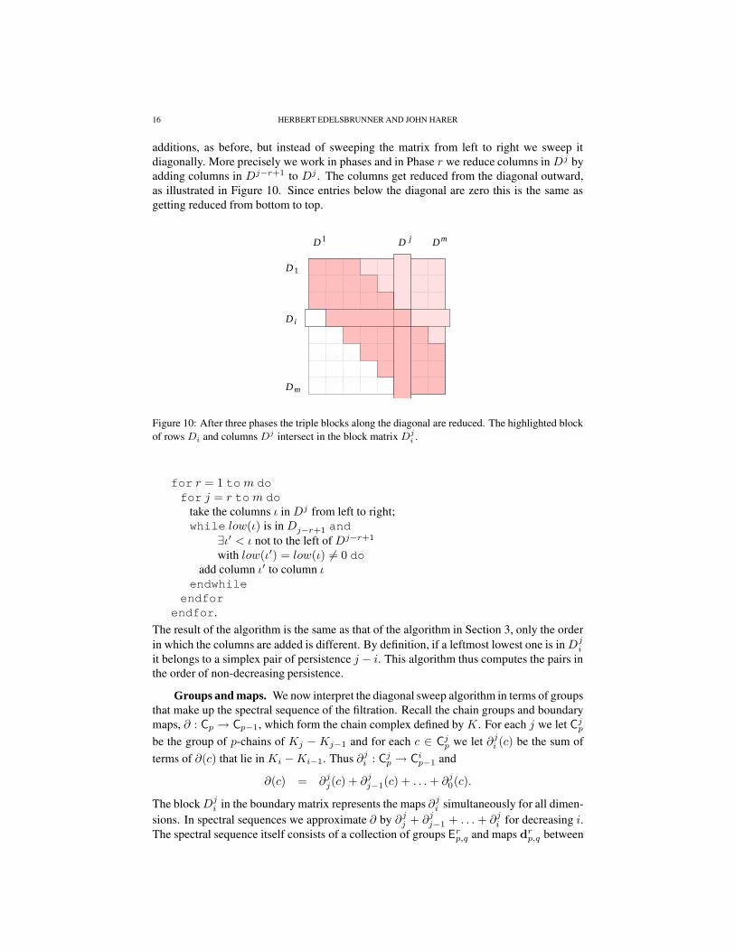
additions, as before, but instead of sweeping the matrix from left to right we sweep itdiagonally. More precisely we work in phases and in Phase r we reduce columns in Dj byadding columns in Dj−r+1 to Dj . The columns get reduced from the diagonal outward,as illustrated in Figure 10. Since entries below the diagonal are zero this is the same asgetting reduced from bottom to top.

DD

D

D

D

D

1

i

m

j1 m

Figure 10: After three phases the triple blocks along the diagonal are reduced. The highlighted blockof rows Di and columns Dj intersect in the block matrix D

ji .

for r = 1 to m dofor j = r to m do

take the columns ι in Dj from left to right;while low(ι) is in Dj−r+1 and

∃ι′ < ι not to the left of Dj−r+1

with low(ι′) = low(ι) 6= 0 doadd column ι′ to column ι

endwhileendfor

endfor.The result of the algorithm is the same as that of the algorithm in Section 3, only the orderin which the columns are added is different. By definition, if a leftmost lowest one is in Dj

i

it belongs to a simplex pair of persistence j − i. This algorithm thus computes the pairs inthe order of non-decreasing persistence.

Groups and maps. We now interpret the diagonal sweep algorithm in terms of groupsthat make up the spectral sequence of the filtration. Recall the chain groups and boundarymaps, ∂ : Cp → Cp−1, which form the chain complex defined by K. For each j we let C

jp

be the group of p-chains of Kj −Kj−1 and for each c ∈ Cjp we let ∂j

i (c) be the sum ofterms of ∂(c) that lie in Ki −Ki−1. Thus ∂j

i : Cjp → C

ip−1 and

∂(c) = ∂jj(c) + ∂j

j−1(c) + . . . + ∂j0(c).

The block Dji in the boundary matrix represents the maps ∂j

i simultaneously for all dimen-sions. In spectral sequences we approximate ∂ by ∂j

j + ∂jj−1 + . . . + ∂j

i for decreasing i.The spectral sequence itself consists of a collection of groups E

rp,q and maps dr

p,q between


them. We follow the customary convention in which the first subscript, p, identifies theblock of columns, the sum of subscripts, p+ q, gives the dimension, and the superscript, r,counts the phases in the iteration. To begin let E0

p,q = Cpp+q and let d0

p,q : E0p,q → E0

p,q−1

be defined by the (p + q)-dimensional boundary map restricted to Dpp , that is, d0

p,q is ∂pp

as applied to (p + q)-chains. It is easy to check that d0p,q−1 ◦ d0

p,q = 0 so we get a set ofvertical chain complexes which we write in a grid:

. . . . . . . . . . . .↓ ↓ ↓ ↓

E01,1 E

02,1 E

03,1 . . .

↓ ↓ ↓ ↓E

01,0 E

02,0 E

03,0 . . .

↓ ↓ ↓ ↓E

01,−1 E

02,−1 E

03,−1 . . .

↓ ↓ ↓E

02,−2 E

03,−2 . . .↓ ↓

E03,−3 . . .

↓. . .

We call this the E0-term of the spectral sequence. The groups E0p,q are generated by the

columns in Dp and the maps d0p,q are represented by the block Dp

p .

Iteration. After interpreting the original boundary matrix we now push this interpre-tation through the phases of the algorithm. For the first phase, we take the homology of theabove vertical complexes and define

E1p,q = kerd0

p,q/imd0p,q+1.

An element of E1p,q is thus the equivalence class of a chain c ∈ C

pp+q with ∂p

p(c) = 0, wheretwo chains are equivalent if their difference lies in the image of ∂p

p , taking of course theboundary map that applies to chains of one higher dimension. In other words, the elementis a relative homology class and more generally E1

p,q ' Hp+q(Kp, Kp−1). Representativesof E1

p,q are computed by reducing the matrix Dpp , which is what the diagonal sweep algo-

rithm does in Phase r = 1. The zero columns in Dpp correspond to positive simplices and

represent cycles. Some are paired and have zero persistence since their classes come andgo within Kp − Kp−1. Others are not paired and their cycles are the generators of E1

p,q .Next we define d1

p,q : E1p,q → E1

p−1,q. Letting γ be a class in E1p,q we set d1

p,q(γ) equal tothe equivalence class of ∂p−1

p (γ) in E1p−1,q . This gives a set of horizontal chain complexes

which we write in a grid as before:

. . . ← . . . ← . . . ← . . .

E11,1 ← E

12,1 ← E

13,1 ← . . .

E11,0 ← E

12,0 ← E

13,0 ← . . .

E11,−1 ← E

12,−1 ← E

13,−1 ← . . .

E12,−2 ← E

13,−2 ← . . .

E13,−3 ← . . .


This is the E1-term of the spectral sequence. We take one more step before appealing toinduction, taking the homology of the horizontal complexes,

E2p,q = kerd1

p,q/imd1p+1,q .

An element of E2p,q is the equivalence class of the sum of a chain c ∈ C

pp+q and an-

other chain c′ ∈ Cp−1p+q . The chains satisfy ∂p

p(c) = 0 and ∂pp−1(c) + ∂p−1

p−1(c′) = 0

and being equivalent means that the difference lies in im ∂pp + im ∂p

p−1 + im ∂p−1p−1 . The

group E2p,q is not a relative homology group by itself but a subgroup of one, namely

E2p,q ⊕ E1

p−1,q+1 ' Hp+q(Kp, Kp−2). Representatives of E2p,q are computed by reduc-

ing the double block of matrices Dpp, Dp−1

p−1 , Dp−1p , Dp

p−1. The first two have already beenreduced and the third is zero. Phase r = 2 completes the reduction of the double block forthe remaining fourth matrix. Next we define d2

p,q : E2p,q → E

2p−2,q+1 which gives another

set of chain complexes.The process continues and for general phase numbers r the map takes r steps to the

left and r−1 steps up, drp,q : Er

p,q → Erp−r,q+r−1. This gives a set of chain complexes and

we take homology to enter the next phase. Since K is finite the maps are eventually zeroand the sequence converges to a limit term, Er = E∞ for r large enough. The homologygroups of K are obtained by taking direct sums along the diagonals in the limit term. Hereit is crucial that we work over a field. Over Z, for example, there are extension problemsto solve because of torsion [5].

6. Stability

An important property of persistence is its stability under perturbations. After for-mulating this concept for continuous functions, we list some of its consequences, whichincludes inequalities for the curvature of smooth curves and surfaces. The stability leads tocontinuous images, called vineyards, that track topological features in homotopies, a newparadigm in the study of dynamic processes.

Bottleneck distance. Let X be a topological space with two tame functions f, g :X → R. We recall that this entails that f and g are continuous, that all sublevel setshave homology groups of finite rank, and that these groups change at a finite number ofhomological critical values. As explained in Section 2, we encode the homology groupsof the sublevel sets in the persistence diagrams Dgmp(f) and Dgmp(g), each a multisetof points in the extended plane, R

2. The L∞-distance between points u = (u1, u2) andv = (v1, v2) in the extended plane is ‖u− v‖

∞= max{|u1 − v1|, |u2 − v2|}, where

the difference between two infinite coordinates is defined to be zero. Given a bijection ηbetween two diagrams, we take the supremum L∞-distance between matched points anddefine the bottleneck distance by taking the infimum over all supremums,

dB(Dgmp(f), Dgmp(g)) = infη

supx‖x− η(x)‖

∞.

Besides the finitely many off-diagonal points, each diagram includes copies of all points onthe diagonal. These are needed for the bijections because the number of off-diagonal pointsin two diagrams is not necessarily the same. As suggested by Figure 11, we may think ofa diagonal point as an anti-cancellation in waiting. Measuring the distance between func-tions by taking the supremum of the absolute difference between corresponding values,‖f − g‖

∞= supx∈X |f(x)− g(x)| we are now ready to state in what sense persistence is

stable.


x

x 2

1

Figure 11: Left: two functions with small L∞-distance. Right: the corresponding two persistencediagrams with small bottleneck distance.

THEOREM 6.1. Let X be a topological space with tame functions f, g : X→ R. Thenfor each dimension p the bottleneck distance between the dimension p persistence diagramsis bounded from above by the difference between the functions, dB(Dgmp(f), Dgmp(g)) ≤‖f − g‖

∞.

The proof given in [13] chases diagrams formed by homomorphisms induced by in-clusions between various sublevel sets of f and g. An alternative elementary proof of aslightly weaker version of the theorem can be found in [15]. A proof for connected com-ponents tracked by the dimension 0 persistence diagram has independently been obtainedin [3].

Applications. The stability of persistence diagrams has a number of consequences,some immediate and some less direct. We restrict ourselves to brief descriptions and asmall number of references.

Homology inference. Let X0 ⊆ Rd be a closed set and write d0 : R

d → R for theEuclidean distance function that maps each point to its Euclidean distance from the nearestpoint in X0. For each ε ≥ 0, the parallel body is a sublevel set of the distance function,Xε

0 = d−10 [0, ε]. Let X1 be another closed set in R

d. The Hausdorff distance betweenthe two sets, dH (X0, X1), is the infimum over all ε for which X0 ⊆ Xε

1 and X1 ⊆Xε

0 . The homological feature size of X0, denoted hfs(X0), is the infimum of the positivehomological critical value of d0. Let dH (X0, X1) < ε < hfs(X0)/4 and δ > 0 sufficientlysmall. Then the rank of the p-dimensional homology group of the parallel body defined byδ is

rankHp(Xδ0 ) = rank im f3ε

ε ,(6.1)

where f3εε : Hp(X

ε1) → Hp(X

3ε1 ) is induced by inclusion. For example X0 could be a

body bounded by a smooth surface and X1 could be a finite point sample of the body. Inthis case the homological feature size is necessarily positive and the result says that we cancompute the homology of the body from a finite sample. In [13] this result is proved asa corollary to the stability theorem. It has been obtained independently in [11]. A similarresult with a stronger requirement on the closeness between X0 and X1 can be found in[38].


Shape comparison. An important problem in practice is measuring the similarity betweenshapes, may it be faces, teeth, plants, tools, or what have you. For i = 0, 1 let Xi ⊆ R

3 anddi : R

3 → R the corresponding distance function on the ambient space. The differencebetween two distance functions is bounded from above by the Hausdorff distance betweenthe shapes,

‖d0 − d1‖∞ ≤ dH(X0, X1).

Theorem 6.1 thus implies that the bottleneck distance between corresponding persistencediagrams is bounded from above by the Hausdorff distance. We remark that the reverseis generally not true. For example, if X1 is the mirror image of the non-symmetric shapeX0 then the two corresponding distance functions have identical persistence diagrams eventhough the Hausdorff distance between the two shapes is non-zero.

A finer function aimed at measuring the difference between smooth surfaces has beenintroduced in [7]. It maps each point and unit tangent vector at the point to the correspond-ing absolute normal curvature. This is a function over the (four-dimensional) tangent bun-dle of the surface. If η : R

3 → R3 is a diffeomorphism that has derivatives up to second

order close to the identity then the bottleneck distance between the persistence diagramsfor the surfaces X and η(X) is small [13].

Curvature of curves. Let γ : S1 → R

2 be a smooth closed curve. Writing κ(s) for the(absolute) curvature at γ(s), the total curvature is

k(γ) =`(γ)

2π

∫s∈S1

κ(s) ds,

where `(γ) is the length. Note that k(γ) is also the distance traveled by the unit tangentvector on the circle of directions. Fary’s Theorem states that if the image of γ is containedin the unit disk then the total curvature cannot be less than the length, `(γ) ≤ k(γ) [28].Using Theorem 6.1, [12] generalizes this to a statement about two smooth curves γ0, γ1 :S

1 → R2. The Frechet distance between them is dF (γ0, γ1) = infϕ sups ‖γ0(s)− γ1(s)‖,

where ϕ ranges over all homeomorphisms between two unit circles and s ranges over allpoints of the first unit circle. Letting `i = `(γi) be the length and ki = k(γi) the totalcurvature, we have

|`0 − `1| ≤ [k0 + k1 − 2π] dF (γ0, γ1).(6.2)

Letting γ0 be the curve inside the unit disk and γ1 a tiny circle around the origin we seethat this inequality indeed implies Fary’s Theorem in the plane. Both Fary’s Theorem and(6.2) generalize to smooth curves in Euclidean spaces of dimension beyond two.

Curvature of surfaces. There is a similar inequality that relates two notions of curvature ofa closed surface X embedded in R

3. Letting κ1(x) ≥ κ2(x) be the principal curvatures ata point x ∈ X , the total mean curvature and the total absolute Gaussian curvature of thesurface are

h(X) =1

2

∫x∈X

(κ1(x) + κ2(x)) dx;

k(X) =

∫x∈X

|κ1(x)κ2(x)| dx.

Since it is embedded the surface necessarily partitions R3 into the bounded set X of points

on and inside X and the unbounded complement of X. Given two surfaces Xi with total


mean curvature hi = h(Xi) and total absolute Gaussian curvature ki = k(Xi), for i =0, 1, we have

|h0 − h1| ≤ [k0 + k1 − 4π(1 + g)] dF (X0, X1),(6.3)where g is the common genus of X0 and X1 and dF is the Frechet distance between thebodies bounded by the surfaces. Recall that this distance is the supremum of ‖x− η(x)‖over all points x ∈ X0 and all homeomorphisms η : X0 → X1. The latter exist becausethe surfaces have the same genus. The proof of the inequality given in [12] uses integralgeometry expressions of the total mean curvature and the total absolute Gaussian curvature.These formulations extend naturally to non-smooth surfaces. The inequality can thus beused to bound the difference between the total mean curvature of a smooth surface and apiecewise linear approximation of that surface.

Time series. So far we have only discussed persistence for single functions. We nowconsider how persistence changes when we have a 1-parameter family of functions. In thiscase the points in the persistence diagrams move in the plane. Sometimes a point appearsor disappears and sometimes two points interact in what we will call a switch. Theorem6.1 limits the changes to continuous motion. The diagrams can therefore be stacked up toform a collection of curves. We explain this in some detail assuming a d-manifold M andtwo Morse functions f0, f1 : M → R. Any two smooth functions can be connected bythe straight-line homotopy and therefore also f0 and f1. In other words, there is a smoothhomotopy F : M× [0, 1]→ R with F (x, 0) = f0(x) and F (x, 1) = f1(x) for all x ∈ M.The thus defined path consists of functions ft(x) = F (x, t) for t from 0 to 1. Furthermore,the path can be deformed slightly to a generic path in which every ft is Morse except at afinite number of times 0 < t1 < . . . < tn < 1 at which either

• two critical points of ftishare the same critical value;

• a critical point x is degenerate with nearby local coordinates under which fti

takes the form fti(y) = fti

(x) + y31 ± y2

2 ± . . .± y2d;

see [10]. The first violation is an interchange of two critical values. The degenerate criticalpoint in the second violation is known as a birth-death point: as ft passes through fti

twonon-degenerate critical points annihilate each other in a cancellation at x (a death) or twonon-degenerate critical points emerge in an anticancellation from x (a birth).

As we follow the generic path of functions the persistence diagram changes in inter-esting ways. As long as the function remains Morse the pairing of critical points does notchange and the off-diagonal points in the diagrams vary continuously. At a death an off-diagonal point merges into the diagonal while at a birth one emerges from the diagonal.At an interchange there are two possibilities depending on whether the pairing changes.Suppose xt and yt are two critical points that go through an interchange at t = ti and be-fore the interchange xt is paired with x′

t and yt is paired with y′

t. Assuming xt and yt areboth positive the points in the diagrams that represent the pairs are ut = (ft(xt), ft(x

′

t))and vt = (ft(yt), ft(y

′

t)). At t = ti the two points line up on a common vertical line.There are now two possibilities. In one case the pairs remain unchanged and the pointsut and vt simply pass one another. In the other case the pairing switches by which wemean that for t > ti the points continue on the trajectories ut = (ft(yt), ft(x

′

t)) andvt = (ft(xt), ft(y

′

t)). Since the switch happens at the moment ut and vt share the samefirst coordinate there is no jump although the speed and direction of the two points under-goes a sudden change. We use the types of xt and yt to distinguish between three kinds ofswitches. It is easy to see that a necessary condition for a switch is that the interchangingcritical points have the same index. We get another, less obvious necessary condition by


++ −

−

++ −

−

++

++

+

+

+

+

−−

−−

−

−−

−

Figure 12: From left to right: a switch between two positive critical points, between two negativecritical points, and between a positive and a negative critical point. In the third case the two inter-changing critical points also swap their types.

interpreting the points ut and vt as two intervals. As proved in [15] a switch requires thatboth before and after the switch the two intervals are nested or disjoint; see Figure 12.

We can track the evolution of the persistence diagram by adding an extra dimensionfor time. The vineyard is the collection of points (ft(xt), ft(x

′

t), t) where the (xt, x′

t) arecritical points paired by persistence. The above analysis shows that the vineyard is a familyof curves that start and end either at off-diagonal locations in the planes t = 0, 1 or on thediagonal wall of points (x, x, t).

Dynamic algorithm. To compute the vineyard of the family ft we use a triangulationK of the manifold and a filtration that changes with t. Interchanges, deaths, and birthsall reduce to transpositions in the compatible ordering of simplices. Such a transpositionmay or may not affect the pairing of simplices. Writing n for the number of simplices,the algorithm in [15] takes time O(n) to decide which case it is and to update the pairingif it is affected by the transposition. To describe the algorithm we let D be the boundarymatrix defined by the ordering of the simplices at time t. Letting R be a correspondingreduced boundary matrix we have R = DV , and since V is invertible we have D = RU ,where U = V −1. We call this an RU-decomposition of D assuming R is reduced andU is upper triangular. The RU-decomposition is not unique but any one defines the samepairing of simplices. To transpose two simplices in the ordering we swap the correspondingrows and columns in D. Equivalently, we multiply D with the permutation matrix fromboth sides giving PDP = (PRP )(PUP ). It fails to be an RU-decomposition if PRP isnot reduced or PUP is not upper triangular. Both shortcomings can be remedied with aconstant number of row and column operations giving an algorithm that takes linear timeper transposition in the worst case; see [15] for details.

In practice it is more efficient to represent both R and U as sparse matrices. To ef-ficiently maintain the pairing requires a slightly richer collection of primitives than com-puting the pairing. We therefore need a sparse matrix data structure that is different fromthe one described in Section 3. To represent R we use two linear arrays, a vertical one toindex the rows and a horizontal one to index the columns. Each column is represented bya singly linked list storing the row numbers of its non-zero entries, as sketched in Figure13. To add two columns we merge the two linked lists while deleting nodes that come induplicate. To swap two columns we swap two pointers in the horizontal array. To swaptwo rows we record the new row positions in the vertical array but do not propagate thatchange to the linked lists. This way the lists remain consistently ordered which simplifiesthe merging since it can be done without reordering. We use a symmetric sparse matrix


Figure 13: The sparse matrix representation of R supports column additions as well as column androw swaps.

implementation for U and get a data structure that takes a constant amount of memory pernon-zero entry in R and in U .

7. Discussion

In spite of its short history, persistent homology has already lead to a number of in-teresting results and connected problems from seemingly distant fields. To substantiatethis view we briefly mention developments that are related to persistence and we draw aspeculative bigger picture by expressing where we believe persistent homology might leadus.

Related developments. We discuss three research directions: the decomposition andsimplification of functions, data analysis and witness complexes, and coverage questionsfor sensor networks.

Morse-Smale complexes and simplification. A Morse function on a Riemannian manifolddefines a gradient flow that can be used to decompose the manifold into regions of con-stant origin or destination. An additional non-degeneracy condition leads to Morse-Smalefunctions which can be used to decompose the manifold into regions of points with com-mon origin and common destination. Both decompositions have applications in medicalimaging [41] and in geometric modeling [20]. A show stopper in these applications isthe over-segmentation resulting from spurious critical points created by noisy data or ar-tifacts of the data representation. There has been work on simplifying the decompositionusing persistent homology for 2-manifolds [22] and for 3-manifolds [21]. Both methodssimplify the decomposition but do not adjust the function that leads to the simplification,which is a more difficult problem. A controlled adjustment of a piecewise linear functionon a 2-manifold that simplifies the persistence diagram by eliminating points of persistencebelow a given threshold while retaining all other points unchanged has been described in[25]. The problem for manifolds of dimension three and higher is still open.

Data analysis and witness complexes. Generalizing a topology preserving network con-struction in [33], de Silva and Carlsson introduced witness complexes by using the majorityof the data as witnesses that support the construction of simplices connecting a minorityof the data points [18]. While there are distinct similarities to other shape reconstruction


methods, see e.g. [2], there are also important differences. Perhaps the most significantdifference is the liberation from the metric of the ambient space. Indeed many data sets ofinterest are preferably interpreted as sampled from or nearby subspaces of positive codi-mension. Without knowing what these subspaces are, the partition of the data into land-marks and witnesses allows us to approximate distances in these subspaces. This liberationfavors the use of coarse landmark sets and permits the exploration of high dimensions. Atthe same time, it suggests we focus on the gross, topological features of the data ratherthan on the fine, geometric distinctions. A good example of this research is the analy-sis of image data leading to the realization that small patches are located on or nearby ahypothetical Klein bottle [8].

Coverage of sensor networks. Here the central problem is deciding whether a collection ofrelatively primitive sensors with limited domains of observation cover a given region. DeSilva and Ghrist use Vietoris-Rips complexes and their homology to decide this questionunder rather weak assumptions on what we know about the location of the sensors [19].These complexes are upward completions of edge skeleta. In Euclidean space the differ-ence between the Vietoris-Rips complex and the Cech complex (the nerve of the sphericalneighborhoods) can be quantified and related to the radius of the neighborhoods. Thisleads to the characterization of coverage in terms of the homology of complexes. Usingpersistence these characterizations can be made robust to fluctuations in the distribution ofsensors and gaps in the coverage.

Future directions. There are many open questions raised by our current understand-ing of persistent homology. One of the most important is the extent to which this theorycan be generalized to a multi-variate situation in which two or more functions characterizethe data. Negative results in this direction can be found in [9]. Questions on a differentscale level are about the relationship between persistence and other broad approaches toproblems in the sciences. We feel that any attempts to answer them would be prematurebut making the question specific might be productive.

Statistics. How different is the approach with persistent homology to high-dimensionaldata analysis from methods in statistics? We think there is a latent symbiotic relationship.The probabilistic aspects of persistence have not yet been explored and similarly persis-tence has not yet been integrated in statistical approaches to data.

Machine learning. A related question is about the connection between persistent homologyand machine learning. Manifold learning is very much part of that discipline and obviouslyconnects to topological ideas and questions of robustness addressed by persistence.

Dynamical systems. It would be interesting to extend persistence from gradient fields togeneral smooth vector fields defined on manifolds. We refer to [35] for an account ofdiscrete methods and combinatorial algorithms in the field. The connection to the idea ofpersistence is still unclear.

References

[1] P. K. AGARWAL, H. EDELSBRUNNER, J. HARER AND Y. WANG. Extreme elevation on a 2-manifold.Discrete Comput. Geom. 36 (2006), 553–572.

[2] N. AMENTA AND M. BERN. Surface reconstruction by Voronoi filtering. Discrete Comput. Geom. 22(1999), 481–504.

[3] M. D’AMICO, P. FROSINI AND C. LANDI. Optimal matching between reduced size functions. Tech. Reportno. 35, DISMI, Universita di Modena e Reggio Emilia (2003).


[4] P. BENDICH, J. HARER AND H. KING. Persistent intersection homology for stratified spaces. Manuscript,Math. Dept., Duke Univ., Durham, North Carolina, 2007.

[5] K. S. BROWN. Cohomology of Groups. Springer-Verlag, New York, 1994.[6] F. CAGLIARI, M. FERRI AND P. POZZI. Size functions from the categorical viewpoint. Acta Appl. Math.

67 (2001), 225–235.[7] G. CARLSSON, A. COLLINS, L. GUIBAS AND A. ZOMORODIAN. Persistence barcodes for shapes. Inter-

nat. J. Shape Modeling (2005).[8] G. CARLSSON, T. ISHKHANOV, V. DE SILVA AND A. ZOMORODIAN. On the local behavior of spaces of

natural images. Internat. J. Comput. Vision, to appear.[9] G. CARLSSON AND A. ZOMORODIAN. The theory of multidimensional persistence. In “Proc. 23rd Ann.

Sympos. Comput. Geom., 2007”, to appear.[10] J. CERF. La stratification naturelle des espaces de fonctions differentiables reelles et le theoreme de la

pseudo-isotopie. Inst. Hautes Etudes Sci. Publ. Math. 39 (1970), 5–173.[11] F. CHAZAL AND A. LIEUTIER. Weak feature size and persistent homology: computing homology of solids

in Rn from noisy point samples. In “Proc. 21st Ann. Sympos. Comput. Geom., 2005”, 255–262.[12] D. COHEN-STEINER AND H. EDELSBRUNNER. Inequalities for the curvature of curves and surfaces. In

“Proc. 21st Ann. Sympos. Comput. Geom., 2005”, 272–277.[13] D. COHEN-STEINER, H. EDELSBRUNNER AND J. HARER. Stability of persistence diagrams. Discrete

Comput. Geom. 37 (2007), 103–120.[14] D. COHEN-STEINER, H. EDELSBRUNNER AND J. HARER. Extending persistence using Poincare and Lef-

schetz duality. Found. Comput. Math., to appear.[15] D. COHEN-STEINER, H. EDELSBRUNNER AND D. MOROZOV. Vines and vineyards by updating persis-

tence in linear time. In “Proc. 22nd Ann. Sympos. Comput. Geom., 2006”, 119–126.[16] M. L. CONNOLLY. Shape complementarity at the hemo-globin albl subunit interface. Biopolymers 25

(1986), 1229–1247.[17] C. J. A. DELFINADO AND H. EDELSBRUNNER. An incremental algorithm for Betti numbers of simplicial

complexes on the 3-sphere. Comput. Aided Geom. Design 12 (1995), 771–784.[18] V. DE SILVA AND G. CARLSSON. Topological estimation using witness complexes. In “Proc. Sympos.

Point-Based Graphics, 2004”, 157–166.[19] V. DE SILVA AND R. GHRIST. Coverage in sensor networks via persistent homology. J. Alg. Geom. Topol-

ogy, to appear.[20] H. EDELSBRUNNER. Surface tiling with differential topology. In “Proc. 3rd Ann. Sympos. Geom. Process.,

2006”, 9–11.[21] H. EDELSBRUNNER AND J. HARER. The persistent Morse complex segmentation of a 3-manifold. Report

rgi-tech-04-066, Geomagic, Research Triangle Park, North Carolina, 2004.[22] H. EDELSBRUNNER, J. HARER AND A. ZOMORODIAN. Hierarchical Morse-Smale complexes for piece-

wise linear 2-manifolds. Discrete Comput. Geom. 30 (2003), 87–107.[23] H. EDELSBRUNNER, D. G. KIRKPATRICK AND R. SEIDEL. On the shape of a set of points in the plane.

IEEE Trans. Inform. Theory IT-29 (1983), 551–559.[24] H. EDELSBRUNNER, D. LETSCHER AND A. ZOMORODIAN. Topological persistence and simplification.

Discrete Comput. Geom. 28 (2002), 511–533.[25] H. EDELSBRUNNER, D. MOROZOV AND V. PASCUCCI. Persistence-sensitive simplification of functions

on 2-manifolds. In “Proc. 22th Ann. Sympos. Comput. Geom., 2006”, 127–134.[26] H. EDELSBRUNNER AND E. P. MUCKE. Three-dimensional alpha shapes. ACM Trans. Graphics 13 (1994),

43–72.[27] H. EDELSBRUNNER AND A. ZOMORODIAN. Computing linking numbers of a filtration. Homology, Ho-

motopy and Applications 5 (2003), 19–37.[28] I. FARY. Sur certaines inegalites geometriques. Acta Sci. Math. Szeged 12 (1950), 117–124.[29] P. FROSINI AND C. LANDI. Size theory as a topological tool for computer vision. Pattern Recognition and

Image Analysis 9 (1999), 596–603.[30] M. GORESKY AND R. MACPHEARSON. Intersection homology I. Topology 19 (1982), 135–162.[31] A. HATCHER. Algebraic Topology. Cambridge Univ. Press, England, 2002.[32] R. KANNAN AND A. BACHEM. Polynomial algorithms for computing the Smith and Hermite normal forms

of an integer matrix. SIAM J. Comput. 8 (1979), 499–507.[33] T. MARTINETZ AND K. SCHULTEN. Topology representing networks. Neural Networks 7 (1994), 507–522.[34] J. MILNOR. Morse Theory. Princeton Univ. Press, New Jersey, 1963.[35] T. KACZYNSKI, K. MISCHAIKOW AND M. MROZEK. Computational Homology. Springer-Verlag, New

York, 2004.


[36] D. MOROZOV. Persistence algorithm takes cubic time in worst case. BioGeometry News, Dept. Comput.Sci., Duke Univ., Durham, North Carolina, 2005.

[37] J. R. MUNKRES. Elements of Algebraic Topology. Addison-Wesley, Redwood City, California, 1984.[38] P. NIYOGI, S. SMALE AND S. WEINBERGER. Finding the homology of submanifolds with high confidence

from random samples. Report TR-2004-08, Dept. Comput. Sci., Univ. Chicago, Illinois, 2004.[39] E. RANNAUD. Persistence in computational topology. Manuscript, Math. Dept., Stanford Univ., California,

2004.[40] V. ROBINS. Toward computing homology from finite approximations. Topology Proceedings 24 (1999),

503–532.[41] J. ROERDINK AND A. MEIJSTER. The watershed transform: definitions, algorithms, and parallelization

strategies. Fundamenta Informaticae 41 (2000), 187–228.[42] G. SEGAL. Classifying spaces and spectral sequences. Inst. Hautes Etudes Sci. Publ. Math. 34 (1968),

105–112.[43] A. STORJOHANN. Near optimal algorithms for computing Smith normal forms of integer matrices. In “Proc.

ACM Sympos. Symbolic Algebraic Comput. 1996”, 267–274.[44] Y. WANG, P. K. AGARWAL, P. BROWN, H. EDELSBRUNNER AND J. RUDOLPH. Coarse and reliable

geometric alignment for protein docking. In “Proc. Pacific Sympos. Biocomput., 2005”, 65–75.[45] A. ZOMORODIAN. Topology for Computing. Cambridge Univ. Press, England, 2005.[46] A. ZOMORODIAN AND G. CARLSSON. Computing persistent homology. Discrete Comput. Geom. 33

(2005), 249–274.[47] A. ZOMORODIAN AND G. CARLSSON. Localized homology. In “Shape Modeling Internat., 2007”, to

appear.

DEPARTMENTS OF COMPUTER SCIENCE AND OF MATHEMATICS, DUKE UNIVERSITY, DURHAM, ANDGEOMAGIC, RESEARCH TRIANGLE PARK, NORTH CAROLINA, USA.

E-mail address: [email protected]

DEPARTMENTS OF MATHEMATICS AND SECTION IN COMPUTATIONAL BIOLOGY AND BIOINFORMAT-ICS, DUKE UNIVERSITY, DURHAM, NORTH CAROLINA, USA.

E-mail address: [email protected]

Persistent Homology — a Surveyv1ranick/papers/edelhare.pdfPersistent Homology — a Survey Herbert...

Documents

Transcript of Persistent Homology — a Surveyv1ranick/papers/edelhare.pdfPersistent Homology — a Survey Herbert...