Perpendicular Intersection

8/8/2019 Perpendicular Intersection

http://slidepdf.com/reader/full/perpendicular-intersection 1/10Copyright (c) 2010 IEEE. Personal use is permitted. For any other purposes, Permission must be obtained from the IEEE by emailing [email protected].

This article has been accepted for publication in a future issue of this journal, but has not been fully edited. Content may change prior to final publication.

1

Perpendicular Intersection: Locating WirelessSensors with Mobile Beacon

Zhongwen Guo, Member, IEEE, Ying Guo, Student Member, IEEE, Feng Hong, Member, IEEE, Zongke

Jin, Yuan He, Student Member, IEEE, Yuan Feng, Member, IEEE, Yunhao Liu, Senior Member, IEEE

Abstract —Existing localization approaches are divided into two groups: range-based and range-free. The range-free schemes often

suffer from poor accuracy and low scalability, while the range-based localization approaches heavily depend on extra hardware

capabilities or rely on the absolute RSSI (received signal strength indicator) values, far from practical. In this work, we propose a mobile-

assisted localization scheme called Perpendicular Intersection (PI), setting a delicate tradeoff between range-free and range-based

approaches. Instead of directly mapping RSSI values into physical distances, by contrasting RSSI values from the mobile beacon to a

sensor node, PI utilizes the geometric relationship of perpendicular intersection to compute node positions. We have implemented the

prototype of PI with 100 TelosB motes and evaluate PI in both indoor and outdoor environments. Through comprehensive experiments,

we show that PI achieves high accuracy, significantly outperforming the existing range-based and the mobile-assisted localization

schemes.

Index Terms —perpendicular intersection, localization, mobile beacon, wireless sensor network.

!

1 INTRODUCTION

L OCATING sensor nodes is a crucial issue and acts as a

fundamental element in wireless sensor network (WSN)

applications [1]. Localization can be classified as range-based

and range-free approaches. Range-free approaches do not

assume the availability or validity of distance information, and

only rely on the connectivity measurements (e.g. hop-count)

from undetermined sensors to a number of seeds [2], [3], [4],

[5]. Having lower requirements on hardware, the accuracy

and precision of range-free approaches are easily affected

by the node densities and network conditions, which are

often unacceptable for many WSN applications that demand

precise localizations. Range-based approaches calculate node

distances based on some measured quantity, such as Time

of Arrival (TOA), Time Difference of Arrival (TDOA) and

Angle of Arrival (AOA) [6], [7], [8], while they usually require

extra hardware support, thus they are expensive in terms of

manufacture cost and energy consumption.

A popular and widely used ranging technique, sometimes

being treated as a “free lunch”, is the received signal strength

(RSS) [6], [9], or quantified as received signal strength in-

dicator (RSSI). The fundamental stumbling block of existing

RSSI-based approaches is that they rely on the absolute RSSIvalues to estimate physical distances [10]. Although being

easy to implement, RSSI-based approaches face many chal-

• Copyright (c) 2010 IEEE. Personal use of this material is permitted. How-ever, permission to use this material for any other purposes must be ob-tained from the IEEE by sending a request to [email protected].

• Zhongwen Guo, Ying Guo, Feng Hong, Zongke Jin, Yuan Feng are withthe department of computer science and engineering of Ocean Universityof China.

E-mail: {guozhw, guoying, hongfeng, jinzongke, fengyuan}@ouc.edu.cn• Yuan He and Yunhao Liu are with the department of computer science and

engineering of Hong Kong University of Science and Technology. E-mail: {heyuan, liu}@cse.ust.hk

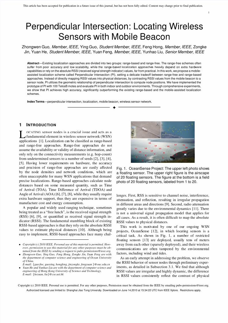
Fig. 1. OceanSense Project: The upper left photo showsa floating sensor. The upper right figure is the airscapeof 20 floating sensors. The figure at the bottom is a fieldphoto of 20 floating sensors, labeled from 1 to 20.

lenges. First, RSS is sensitive to channel noise, interference,

attenuation, and reflection, resulting in irregular propagation

in different areas and directions [9]. Second, radio attenuation

greatly varies due to the environmental dynamics [11]. There

is not a universal signal propagation model that applies for

all cases. As a result, it is often difficult to map the absolute

RSSI values to physical distances.

This work is motivated by one of our ongoing WSNprojects, OceanSense [12], in which locating sensors is a

critical task. As shown in Fig. 1, a number of restricted

floating sensors [13] are deployed, usually tens of meters

away from each other (sparsely deployed), and their wireless

communications are often tampered by the environmental

factors, including wind and tides.

As an early attempt in addressing the problem, we observe

the RSSI behavior of sensor nodes through preliminary exper-

iments, as detailed in Subsection 3.1. We find that although

RSSI values are irregular and highly dynamic, the difference

in RSSI values consistently reflect the contrast of physical

Authorized licensed use limited to: Shanghai Jiao Tong University. Downloaded on June 14,2010 at 15:34:22 UTC from IEEE Xplore. Restrictions apply.


http://slidepdf.com/reader/full/perpendicular-intersection 2/10

Copyright (c) 2010 IEEE. Personal use is permitted. For any other purposes, Permission must be obtained from the IEEE by emailing [email protected].


2

distances. In other words, for the same pair of sensors, a

sender and a receiver, when one of them is moving closer

to the other, in most cases, if not all, the measured RSSI

keeps increasing, although not in a smooth manner. Based on

this observation, we propose Perpendicular Intersection (PI),

a RSSI-based localization scheme using mobile beacon [14].

Major contributions of this paper are as follows:

•

In order to avoid errors from directly mapping absoluteRSSI values to distances, we obtain the geometrical

relationship of sensors by contrasting the measured RSSI

values. We then design a novel localization scheme, PI,

which has better accuracy and low overhead, especially

under dynamic and complex environments.

• We design the optimal trajectory of the mobile beacon in

PI and theoretically prove its correctness. Only one mo-

bile beacon is needed to broadcast beacon signals in PI,

and other sensor nodes simply listen to the signals, store

a few necessary packets, and compute their coordinates

without interfering with each other.

• We implement a prototype of PI with 100 sensors, and

evaluate its performance in real environments, includingindoor and outdoor spots. We show the advantages of this

design through comprehensive experimental results.

The rest of the paper is organized as follows. Section

2 summarizes the related works in localization of WSNs.

Section 3 presents our observations of RSSI and elaborates

the design of PI. Section 4 presents our implementation and

the experimental results. We conclude the work in Section 5.

2 RELATED WOR K

Many approaches have been proposed to determine sensor

node locations, falling into two categories: range-based ap-

proaches and range-free approaches.

2.1 Range-Based Approaches

Range-based approaches assume that sensor nodes are able

to measure the distance and/or the relative directions of

neighbor nodes. Various techniques are employed to measure

the physical distance. For examples, TOA obtains range infor-

mation via signal propagation times [6], and TDOA estimates

the node locations by utilizing the time differences among

signals received from multiple senders [7]. As an extension of

TOA and TDOA, AOA allows nodes to estimate the relative

directions between neighbors by setting an antenna array

for each node [8]. All those approaches require expensivehardware. For example, TDOA needs at lest two different

signal generators [7]. AOA needs antenna array and multiple

ultrasonic receivers [8].

RSSI is utilized to estimate the distance between two nodes

with ordinary hardware [6], [9]. Various theoretical or empir-

ical models of radio signal propagation have been constructed

to map absolute RSSI values into estimated distances [10].

The accuracy and precision of such models, however, are far

from perfect. Factors like multi-path fading and background

interference often result in inaccurate range estimations [9],

[11].

Recently, mobile-assisted localization approaches have been

proposed to improve the efficiency of range-based ap-

proaches [15], [16]. The location of a sensor node can be cal-

culated with the range measurements from the mobile beacon

to itself, so no interaction is required between nodes, avoiding

cumulative errors of coordinate calculations and unnecessary

communication overhead. The localization accuracy can also

be improved via multiple measurements obtained when the

mobile beacons are at different positions.

2.2 Range-Free Approaches

Knowing the hardware limitations and energy constraints re-

quired by range-based approaches, researchers propose range-

free solutions as cost-effective alternatives.

Having no distances among nodes, range-free approaches

depend on the connectivity measurements from sensor nodes

to a number of reference nodes, called seeds. For example, in

Centroid [2], seeds broadcast their positions to their neighbor

nodes that record all received beacons. Each node estimates

its location by calculating the center of all seeds it hears.

In APIT [3], each node estimates whether it resides inside

or outside several triangular regions bounded by the seeds

it hears, and refines the computed location by overlapping

such regions. As an alternate solution, DV-HOP only makes

use of constant number of seeds [4]. Instead of single hop

broadcasts, seeds flood their locations throughout the network,

maintaining a running hop-count at each node along the path.

Nodes calculate their positions based on the received seed

locations, the hop-counts from the corresponding anchors, and

the average-distance per hop through trilateration.

Instead of using the absolute RSSI values, by contrasting

the measured RSSI values from the mobile beacon to a sensor

node, our proposed PI utilizes the geometric relationship of

perpendicular intersection to compute the position of the node.

In this sense, PI is actually between range-based and range-

free approaches.

3 DESIGN OF PI

In this section, we first describe the experimental observations

on RSSI, which motivated this design. Subsection 3.2 presents

the overview of PI design. Subsection 3.3 discusses the optimal

trajectory of the mobile beacon for PI. Subsection 3.4 presents

our localization scheme in detail. Subsection 3.5 further in-

troduces the extended design of PI, using random mobile

trajectories for localization. For convenience of expression,

the terms “location”, “position” and “coordinates” are used

interchangeably in the rest of this paper.

3.1 Observations on RSSI

RSSI is initially used for power control in wireless networks.

The existing signal propagation models of RSSI, however, are

far from perfect, mainly because of the uncertain influences

such as background interference, non-uniform spreading, sig-

nal fading and reflections. To better understand RSSI patterns,

we conduct some initial experiments with 12 TelosB sensors

on our campus, as illustrated in Fig. 2(a).






3

(a)

−15 −10 −5 0 5 10 15210

215

220

225

230

235

240

245

250

Distance Interval (m)

R S S I

10m20m

30m

40m50m

(b)

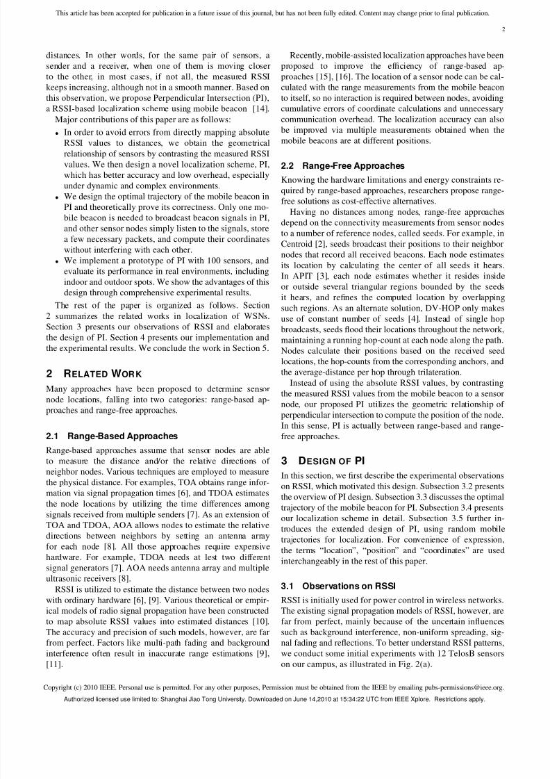
Fig. 2. Observations of RSSI outdoor: (a) deployment sketch (b) RSSI values of the received signals.

In the first group of experiments, node A broadcasts signals,

and the rest nodes receive RSSI values from their CC2420

transceivers. Node A moves from 10 meters away from O to

20, 30, 40, and 50 meters. All the measured RSSI values are

shown in Fig. 2(b).

With the RSSI values from node A to a node, in ideal

sense the distance between other nodes and node A should

be calculated according to the log-normal shadowing model in

Equation (1), which is widely used in range-based localization

approaches [6], [10].

RSSI (d) = P T − P L(d0) − 10ηlog10d

d0+ X σ, (1)

where P T is the transmission power, P L(d0) is the path

loss for a reference distance of d0, and η is the path loss

exponent. The random variation in RSSI is expressed as a

Gaussian random variable X σ = N (0, σ2). All powers are

in dBm and all distances are in meters. η is set between 2and 5. σ is set between 4 and 10, depending on the specific

environment [10].

In Table 1 we compare the real distances between node

A and O with those estimated ones using Equation (1). The

average relative error of estimation is 9.06%.

TABLE 1Results of outdoor observation (m)

|AO| 10 20 30 40 50

Estimated distance 9.62 19.19 30.41 34.12 60.68

Similar results are observed in an indoor environment. Weconduct the second group of experiments in our laboratory.

Node A moves from 4 meters away from O to 8, 12 and 16meters. Table 2 lists the real distances between A and O and

those estimated ones using Equation (1). The average relative

error of estimation is 10.09%.

TABLE 2Results of indoor observation (m)

|AO| 4 8 12 16

Estimated distance 4.76 6.66 11.27 17.94

The above observations reveal that distance estimations

based on the log-normal shadowing model and absolute RSSI

values have very poor accuracy, which results in unacceptable

localization errors in WSNs.

Interestingly, we find that the closer a node is to the signal

sender, the larger RSSI value it perceives. In other words,

although RSSI is irregular in practice, it is usually a fact that

the RSSI between two nodes monotonically decreases as the

nodes become farther from each other. This simple observation

motivates our design of PI. Instead of directly mapping RSSI

values into physical distances, PI locates the nodes by contrast-

ing the RSSI values and utilizing the geometric relationship

among the nodes.

3.2 Perpendicular Intersection

In our experiment, when the mobile beacon moves along a

straight line, the largest RSSI value received by a sensor node

often, if not always, corresponds to the point on the line

that is closest to the node. Theoretically, this point shouldbe the projection of the node on the line. Given two different

projections of the sensor node on the trajectory, this node can

be located as the intersection point of two perpendiculars that

cross the mobile beacon’s trajectory over the two projections,

respectively.

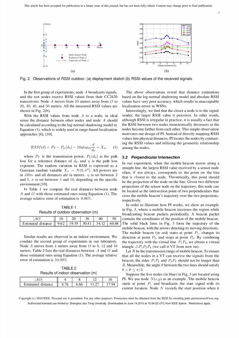
In order to illustrate how PI works, we show an example

in Fig. 3, where a mobile beacon traverses the region while

broadcasting beacon packets periodically. A beacon packet

contains the coordinates of the position of the mobile beacon.

The solid black lines in Fig. 3 form the trajectory of the

mobile beacon, with the arrows denoting its moving directions.

The mobile beacon (in red) starts at point P 1, changes its

direction at point P 2, and stops at point P 3. By combiningthe trajectory with the virtual line P 1P 3, we obtain a virtual

triangle P 1P 2P 3 (we call it VT from now on).

Let R be the transmission range of mobile beacon. To ensure

that all the nodes in a VT can receive the signals from the

beacon, the sides P 1P 2 and P 2P 3 should not be longer than

R. Meanwhile, the angle θ between the two lines should satisfy

0 < θ ≤ π/3.

Suppose the five nodes (in blue) in Fig. 3 are located using

PI. We use node N (x,y) as an example. The mobile beacon

starts at point P 1 and broadcasts the start signal with its

current location. Node N records the start position when it






4

Fig. 3. An example of PI scheme.

hears the start signal. Along its trajectory from P 1 to P 2, the

mobile beacon broadcasts beacon packets periodically with

its current location. Node N receives all the beacon packets,

and records the one with the largest RSSI value. When the

mobile beacon arrives at P 2, it broadcasts a stop signal with

its current location. When node N receives the stop packet,

it knows that the mobile beacon has just finished traversing

the line from P 1 to P 2. The recorded position is the position

where the beacon packet with largest RSSI value broadcast.

We label the recorded position as A(x,y).

According to the observations in Subsection 3.1, line seg-

ment N A is the shortest one among all the line segments

connecting node N and any point on line P 1P 2. In other

words, point A is the projection of node N on line P 1P 2.

Hence, line N A is perpendicular to line P 1P 2, and we have:

y2 − y1x2 − x1

×y − y

x− x= −1. (2)

Similarly, when the mobile beacon moves from P 2 to P 3,

another position B(x, y) is recorded which is the projection

of node N on line P 2P 3. Thus we have:

y3 − y2x3 − x2

×y − y

x− x= −1. (3)

By solving Formulas (2) and (3), we can compute the

coordinates (x,y) of node N :

xy

=

x2 − x1 y2 − y1x3 − x2 y3 − y2

−1

× M, (4)

where

M =

x2 − x1 y2 − y1 0 0

0 0 x3 − x2 y3 − y2

x

y

x

y

.

In the above process, we only contrast the RSSI values and

utilize the geometric relationship among the nodes and the

beacon to do localization. The location calculation does not

require any absolute values of RSSI, nor does it base on any

signal propagation model. In this way, PI is expected to avoid

the potential errors generated from the translations from RSSI

to distances.

3.3 Optimal Trajectory

Clearly, a sensor node can be easily located when it is in

the scope of a VT. When the entire deployment area of a

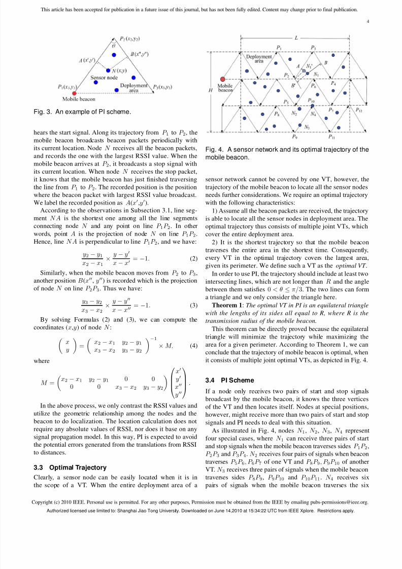
Fig. 4. A sensor network and its optimal trajectory of themobile beacon.

sensor network cannot be covered by one VT, however, the

trajectory of the mobile beacon to locate all the sensor nodes

needs further considerations. We require an optimal trajectory

with the following characteristics:

1) Assume all the beacon packets are received, the trajectory

is able to locate all the sensor nodes in deployment area. The

optimal trajectory thus consists of multiple joint VTs, which

cover the entire deployment area.

2) It is the shortest trajectory so that the mobile beacon

traverses the entire area in the shortest time. Consequently,

every VT in the optimal trajectory covers the largest area,

given its perimeter. We define such a VT as the optimal VT .

In order to use PI, the trajectory should include at least two

intersecting lines, which are not longer than R and the angle

between them satisfies 0 < θ ≤ π/3. The two lines can form

a triangle and we only consider the triangle here.Theorem 1: The optimal VT in PI is an equilateral triangle

with the lengths of its sides all equal to R, where R is the

transmission radius of the mobile beacon.

This theorem can be directly proved because the equilateral

triangle will minimize the trajectory while maximizing the

area for a given perimeter. According to Theorem 1, we can

conclude that the trajectory of mobile beacon is optimal, when

it consists of multiple joint optimal VTs, as depicted in Fig. 4.

3.4 PI Scheme

If a node only receives two pairs of start and stop signals

broadcast by the mobile beacon, it knows the three verticesof the VT and then locates itself. Nodes at special positions,

however, might receive more than two pairs of start and stop

signals and PI needs to deal with this situation.

As illustrated in Fig. 4, nodes N 1, N 2, N 3, N 4 represent

four special cases, where N 1 can receive three pairs of start

and stop signals when the mobile beacon traverses sides P 1P 2,

P 2P 3 and P 3P 4. N 2 receives four pairs of signals when beacon

traverses P 5P 6, P 6P 7 of one VT and P 8P 9, P 9P 10 of another

VT. N 3 receives three pairs of signals when the mobile beacon

traverses sides P 8P 9, P 9P 10 and P 10P 11. N 4 receives six

pairs of signals when the mobile beacon traverses the six






5

OnMessageReceived(Message m){if (m.flag==start){ // start of side(i)

side.clear(); // clear the variable side(i-1)

Record(side.start,m);

// save RSSI and position of the

// first beacon signal on side(i)

rssimax=m.RSSI; positionmax=m.position;

}else if ((m.flag==beacon)and(m.RSSI≥rssimax)){

// larger RSSI, update current // rssimax and positionmax

rssimax=m.RSSI; positionmax=m.position;

}else if (m.flag==stop){ // end of side(i)

Record(side.stop,m);

side(i)=side; cp(i)=positionmax;

if (side(i-1).stop==side(i).start){loc=calculate(side(i-1),side(i));

// keep the one with the largest SumRSSI (),

// if multiple location results exist

if ((loc!=location) and (SumRSSI(loc)

>SumRSSI(location)))

location=loc;

}}

}

Fig. 5. PI algorithm.

sides of four VTs P 5P 6P 7, P 8P 9P 10, P 9P 10P 11 and

P 10P 11P 12.

If a node receives start and stop signals from all the three

vertices of a VT, we call this VT a locating VT for the

node. For example in Fig. 4, P 2P 3P 4 is the locating VT for

node N 1, because node N 1 can receive start and stop signals

from P 2, P 3 and P 4. PI lets each node compute the sum of RSSI values from the three vertices of a locating VT, and

the locating VT whose vertices have the largest sum of RSSI

values is used to calculate the node location.

The pseudo code of the main function on message pro-

cessing in PI is shown in Fig. 5. We define side(i) (1≤i≤6)

as the side from which the node receives the ith pair of

start and stop signals. Let cp(i) denote the point on side(i)

that is closest to the node. Variable side denotes the current

side traversed by the mobile beacon. Variable rssimax and

positionmax respectively denote the current largest RSSI

value and its corresponding beacon position. Variable loc

denotes the location calculated from the current locating VT.

The final result of the node coordinates is stored in the variablelocation. SumRSSI ( p) calculates the sum of RSSI values

from the three vertices of the position p’s locating VT.

PI can address all the special cases. For example, N 1receives three pairs of start and stop signals, respectively

from the locating VTs P 1P 2P 3 and P 2P 3P 4, so the

corresponding calculated results by using these two locating

VTs are the coordinates of points N 1

and N 1. For a node

at point N 1, P 2P 3P 4 has larger sum of RSSI values than

P 1P 2P 3. Thus, the coordinates of point N 1 can be correctly

selected in place of the coordinates of N 1

. Similarly, nodes

N 2, N 3 and N 4 can determine their coordinates from multiple

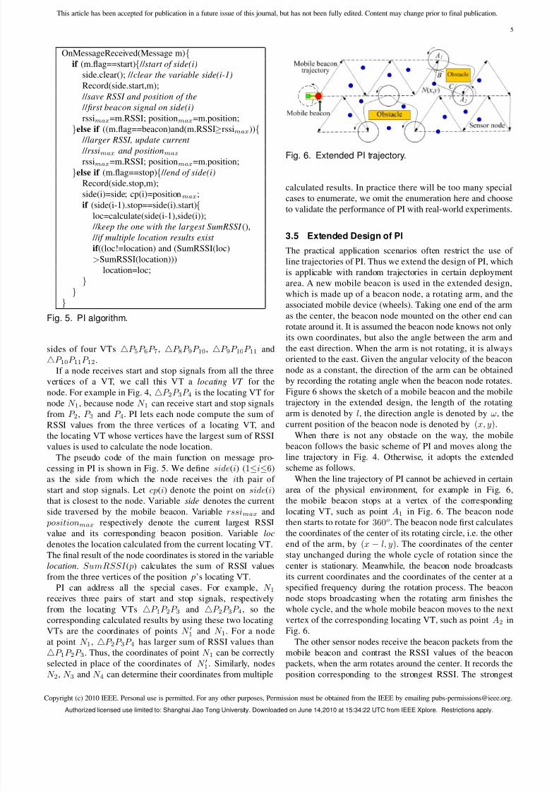
Fig. 6. Extended PI trajectory.

calculated results. In practice there will be too many special

cases to enumerate, we omit the enumeration here and choose

to validate the performance of PI with real-world experiments.

3.5 Extended Design of PI

The practical application scenarios often restrict the use of

line trajectories of PI. Thus we extend the design of PI, which

is applicable with random trajectories in certain deployment

area. A new mobile beacon is used in the extended design,

which is made up of a beacon node, a rotating arm, and the

associated mobile device (wheels). Taking one end of the arm

as the center, the beacon node mounted on the other end can

rotate around it. It is assumed the beacon node knows not only

its own coordinates, but also the angle between the arm and

the east direction. When the arm is not rotating, it is always

oriented to the east. Given the angular velocity of the beacon

node as a constant, the direction of the arm can be obtained

by recording the rotating angle when the beacon node rotates.

Figure 6 shows the sketch of a mobile beacon and the mobile

trajectory in the extended design, the length of the rotating

arm is denoted by l, the direction angle is denoted by ω, thecurrent position of the beacon node is denoted by (x, y).

When there is not any obstacle on the way, the mobile

beacon follows the basic scheme of PI and moves along the

line trajectory in Fig. 4. Otherwise, it adopts the extended

scheme as follows.

When the line trajectory of PI cannot be achieved in certain

area of the physical environment, for example in Fig. 6,

the mobile beacon stops at a vertex of the corresponding

locating VT, such as point A1 in Fig. 6. The beacon node

then starts to rotate for 360o. The beacon node first calculates

the coordinates of the center of its rotating circle, i.e. the other

end of the arm, by (x − l, y). The coordinates of the center

stay unchanged during the whole cycle of rotation since thecenter is stationary. Meanwhile, the beacon node broadcasts

its current coordinates and the coordinates of the center at a

specified frequency during the rotation process. The beacon

node stops broadcasting when the rotating arm finishes the

whole cycle, and the whole mobile beacon moves to the next

vertex of the corresponding locating VT, such as point A2 in

Fig. 6.

The other sensor nodes receive the beacon packets from the

mobile beacon and contrast the RSSI values of the beacon

packets, when the arm rotates around the center. It records the

position corresponding to the strongest RSSI. The strongest






6

RSSI theoretically corresponds to a point on the circle, which

is closest to the node to be located. In other words, the circle

center, the beacon node at that point, and the node to be located

are collinear.

For example, node N (x, y) is a node to be located in Fig. 6.

When the center of the rotation circle is A1(x1, y1), node N records the strongest RSSI when the beacon node is at position

B(xb, yb). Thus we have

y − y1yb − y1

=x− x1

xb − x1

, (5)

Similarly, when the center of the rotation circle is

A2(x2, y2), the strongest RSSI corresponds to position

C (xc, yc). We have:

y − y2yc − y2

=x− x2

xc − x2

. (6)

By solving Formulas (5) and (6), we get the coordinates of

node N .

xy

= y1 − yb x1 − xb

y2 − yc x2 − xc−1

× M, (7)

where

M =

y1 − yb x1 − xb 0 0

0 0 y2 − yc x2 − xc

x1

y1x2

y2

.

4 PERFORMANCE EVALUATION

To better evaluate the PI design, we implement a prototype

system of PI with 100 TelosB sensors in various environments,

including library hall, laboratory, racket court, parking lots,

grassplot and sea surface. The mobile beacon is also a TelosBmote which moves manually. The beacon node keeps record-

ing the movement speed (a constant in our experiments) and

the time it has run for, which can be used to calculate its own

current position. A sink is deployed to collect the localization

results of all the sensor nodes.

We evaluate the performance of PI in six different envi-

ronments, and compare it with two other RSSI-based local-

ization approaches: a range-based approach of trilateration

and a mobile-assisted localization approach, which are briefly

introduced as follows.

In the range-based approach of trilateration (called TRL

in short) [17], beacon packets from the three vertices of the

locating VT where the node resides, are used to calculate itslocation. As for the mobile-assisted localization approach, it

exploits Bayesian inference to improve the estimation accu-

racy [15]. We call that approach BI. Six beacon packets are

used in the computation process of BI. Three of them are sent

from the three vertices of the locating VT where the node

resides, while the other three are chosen randomly from the

positions on the two sides of that VT. Both approaches rely

on the signal propagation model of Equation (1) to transform

absolute RSSI values to physical distances.

We obtain the appropriate settings of the parameters in

Equation (1) through measurements beforehand [10]. All the

(a)

0 50 100 150 200 250 300200

210

220

230

240

250

260

R S S I

Time(s)

(b)

1 2 3 4 5 6 7 8 9 10 11 12 13 140

1

2

3

4

5

6

7

Node ID

L o c a t i o n E r r o r ( m )

PI Error

BI Error

TRL Error

Average PI Error

Average BI Error

Average TRL Error

(c)

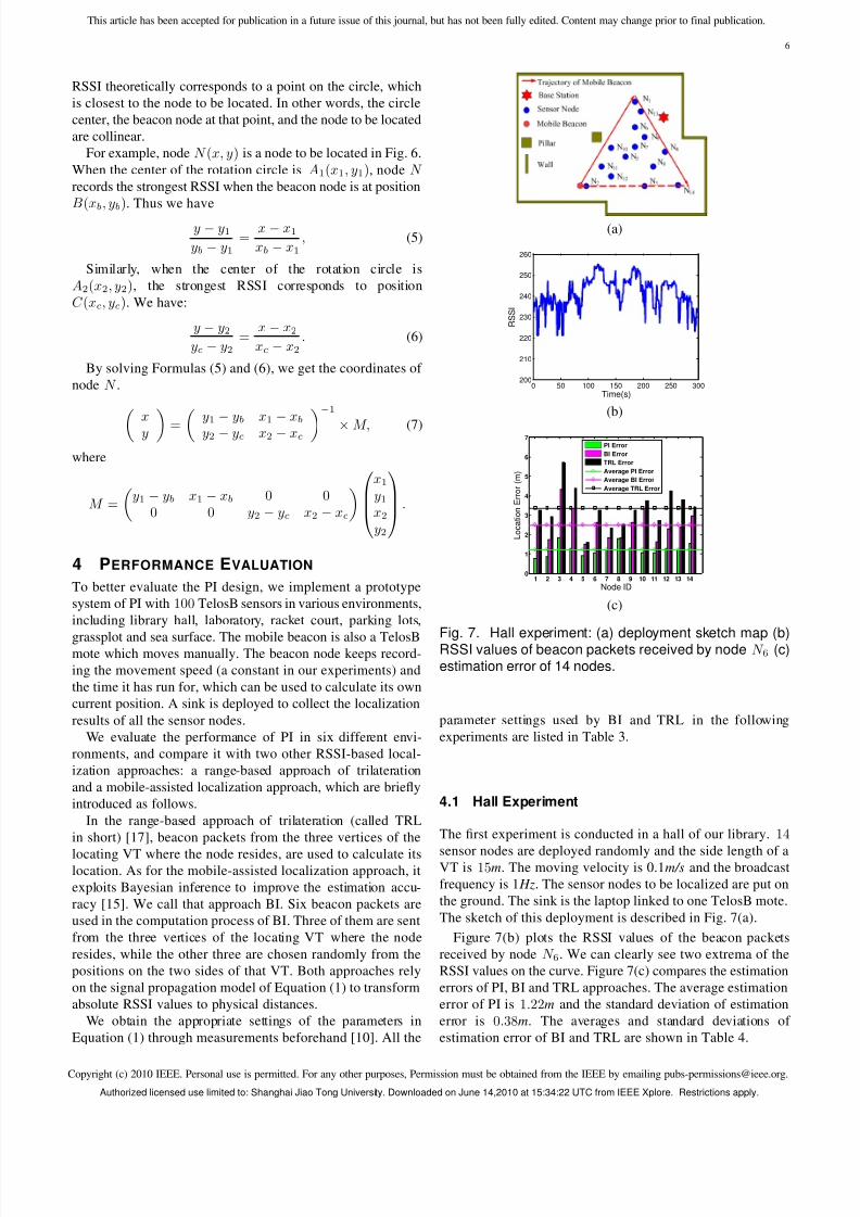
Fig. 7. Hall experiment: (a) deployment sketch map (b)RSSI values of beacon packets received by node N 6 (c)estimation error of 14 nodes.

parameter settings used by BI and TRL in the following

experiments are listed in Table 3.

4.1 Hall Experiment

The first experiment is conducted in a hall of our library. 14

sensor nodes are deployed randomly and the side length of aVT is 15m. The moving velocity is 0.1m/s and the broadcast

frequency is 1 Hz. The sensor nodes to be localized are put on

the ground. The sink is the laptop linked to one TelosB mote.

The sketch of this deployment is described in Fig. 7(a).

Figure 7(b) plots the RSSI values of the beacon packets

received by node N 6. We can clearly see two extrema of the

RSSI values on the curve. Figure 7(c) compares the estimation

errors of PI, BI and TRL approaches. The average estimation

error of PI is 1.22m and the standard deviation of estimation

error is 0.38m. The averages and standard deviations of

estimation error of BI and TRL are shown in Table 4.






7

(a) (b)

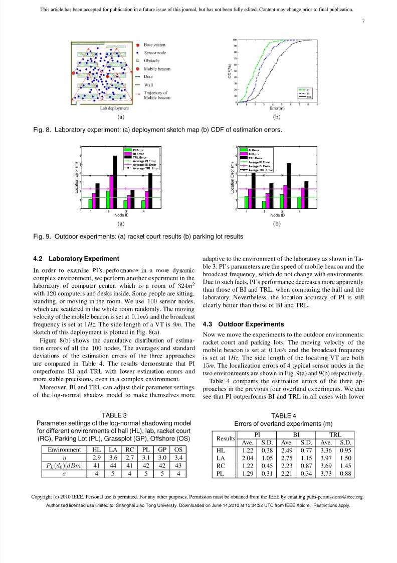
Fig. 8. Laboratory experiment: (a) deployment sketch map (b) CDF of estimation errors.

1 2 3 40

1

2

3

4

5

6

7

Node ID


PI Error

BI Error

TRL Error

Average PI Error

Average BI Error

Average TRL Error

(a)

1 2 3 40

1

2

3

4

5

6

7

Node ID


PI Error

BI Error

TRL Error

Averge PI Error

Averge BI Error

Averge TRL Error

(b)

Fig. 9. Outdoor experiments: (a) racket court results (b) parking lot results

4.2 Laboratory Experiment

In order to examine PI’s performance in a more dynamic

complex environment, we perform another experiment in the

laboratory of computer center, which is a room of 324m2

with 120 computers and desks inside. Some people are sitting,standing, or moving in the room. We use 100 sensor nodes,

which are scattered in the whole room randomly. The moving

velocity of the mobile beacon is set at 0.1m/s and the broadcast

frequency is set at 1 Hz. The side length of a VT is 9m. The

sketch of this deployment is plotted in Fig. 8(a).

Figure 8(b) shows the cumulative distribution of estima-

tion errors of all the 100 nodes. The averages and standard

deviations of the estimation errors of the three approaches

are compared in Table 4. The results demonstrate that PI

outperforms BI and TRL with lower estimation errors and

more stable precisions, even in a complex environment.

Moreover, BI and TRL can adjust their parameter settings

of the log-normal shadow model to make themselves more

TABLE 3Parameter settings of the log-normal shadowing modelfor different environments of hall (HL), lab, racket court(RC), Parking Lot (PL), Grassplot (GP), Offshore (OS)

Environment HL LA RC PL GP OS

η 2.9 3.6 2.7 3.1 3.0 3.4

P L(d0)[dBm] 41 44 41 42 42 43

σ 4 5 4 5 5 4

adaptive to the environment of the laboratory as shown in Ta-

ble 3. PI’s parameters are the speed of mobile beacon and the

broadcast frequency, which do not change with environments.

Due to such facts, PI’s performance decreases more apparently

than those of BI and TRL, when comparing the hall and the

laboratory. Nevertheless, the location accuracy of PI is stillclearly better than those of BI and TRL.

4.3 Outdoor Experiments

Now we move the experiments to the outdoor environments:

racket court and parking lots. The moving velocity of the

mobile beacon is set at 0.1m/s and the broadcast frequency

is set at 1 Hz. The side length of the locating VT are both

15m. The localization errors of 4 typical sensor nodes in the

two environments are shown in Fig. 9(a) and 9(b) respectively.

Table 4 compares the estimation errors of the three ap-

proaches in the previous four overland experiments. We can

see that PI outperforms BI and TRL in all cases with lower

TABLE 4

Errors of overland experiments (m)

ResultsPI BI TRL

Ave. S.D. Ave. S.D. Ave. S.D.

HL 1.22 0.38 2.49 0.77 3.36 0.95

LA 2.04 1.05 2.75 1.15 3.97 1.50

RC 1.22 0.45 2.23 0.87 3.69 1.45

PL 1.29 0.31 2.21 0.34 3.73 0.88






8

(a)

1 2 3 4 5 6 7 8 90

1

2

3

4

5

6

7

Node ID


PI Error

BI Error

TRL Error

Averge PI Error

Averge BI Error

Averge TRL Error

(b)

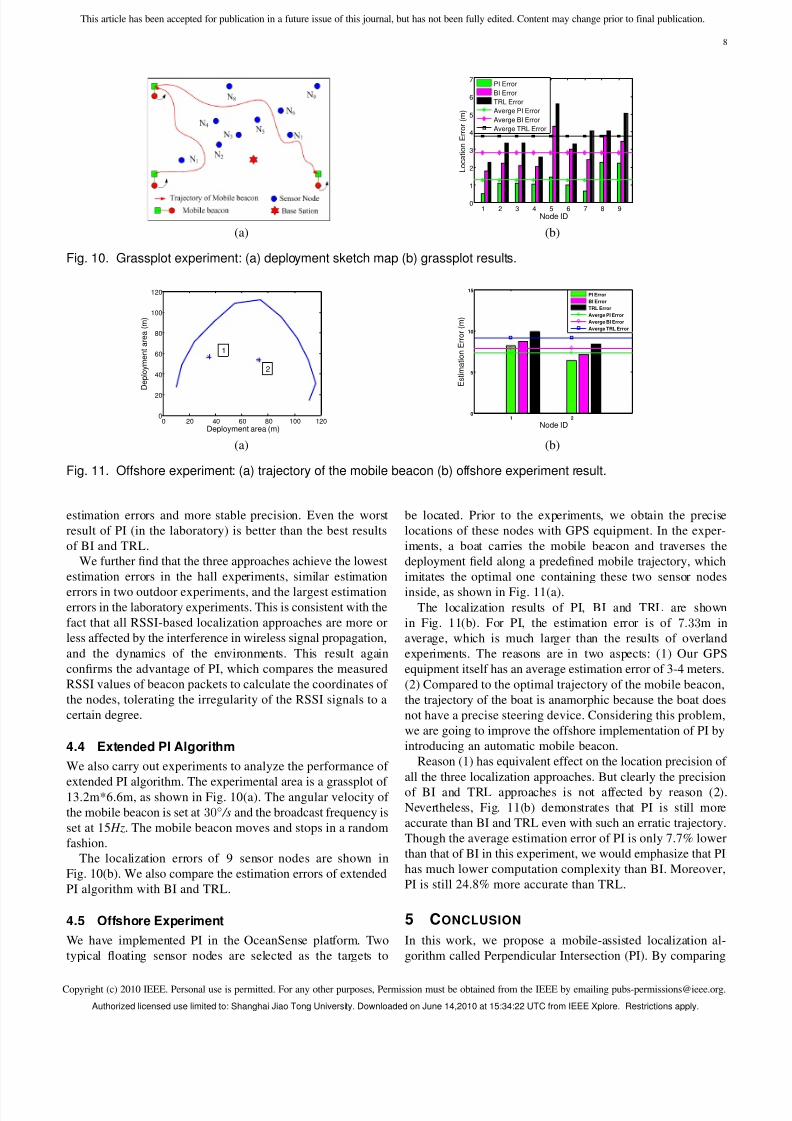
Fig. 10. Grassplot experiment: (a) deployment sketch map (b) grassplot results.

0 20 40 60 80 100 1200

20

40

60

80

100

120

Deployment area (m)

D e p l o y m e n t a r e a ( m )

1

2

(a)

1 20

5

10

15

Node ID

E s t i m a t i o n E r r o r ( m )

PI Error

BI Error

TRL Error

Averge PI Error

Averge BI Error

Averge TRL Error

(b)

Fig. 11. Offshore experiment: (a) trajectory of the mobile beacon (b) offshore experiment result.

estimation errors and more stable precision. Even the worst

result of PI (in the laboratory) is better than the best results

of BI and TRL.

We further find that the three approaches achieve the lowest

estimation errors in the hall experiments, similar estimation

errors in two outdoor experiments, and the largest estimationerrors in the laboratory experiments. This is consistent with the

fact that all RSSI-based localization approaches are more or

less affected by the interference in wireless signal propagation,

and the dynamics of the environments. This result again

confirms the advantage of PI, which compares the measured

RSSI values of beacon packets to calculate the coordinates of

the nodes, tolerating the irregularity of the RSSI signals to a

certain degree.

4.4 Extended PI Algorithm

We also carry out experiments to analyze the performance of

extended PI algorithm. The experimental area is a grassplot of 13.2m*6.6m, as shown in Fig. 10(a). The angular velocity of

the mobile beacon is set at 30◦ /s and the broadcast frequency is

set at 15 Hz. The mobile beacon moves and stops in a random

fashion.

The localization errors of 9 sensor nodes are shown in

Fig. 10(b). We also compare the estimation errors of extended

PI algorithm with BI and TRL.

4.5 Offshore Experiment

We have implemented PI in the OceanSense platform. Two

typical floating sensor nodes are selected as the targets to

be located. Prior to the experiments, we obtain the precise

locations of these nodes with GPS equipment. In the exper-

iments, a boat carries the mobile beacon and traverses the

deployment field along a predefined mobile trajectory, which

imitates the optimal one containing these two sensor nodes

inside, as shown in Fig. 11(a).The localization results of PI, BI and TRL are shown

in Fig. 11(b). For PI, the estimation error is of 7.33m in

average, which is much larger than the results of overland

experiments. The reasons are in two aspects: (1) Our GPS

equipment itself has an average estimation error of 3-4 meters.

(2) Compared to the optimal trajectory of the mobile beacon,

the trajectory of the boat is anamorphic because the boat does

not have a precise steering device. Considering this problem,

we are going to improve the offshore implementation of PI by

introducing an automatic mobile beacon.

Reason (1) has equivalent effect on the location precision of

all the three localization approaches. But clearly the precision

of BI and TRL approaches is not affected by reason (2).

Nevertheless, Fig. 11(b) demonstrates that PI is still more

accurate than BI and TRL even with such an erratic trajectory.

Though the average estimation error of PI is only 7.7% lower

than that of BI in this experiment, we would emphasize that PI

has much lower computation complexity than BI. Moreover,

PI is still 24.8% more accurate than TRL.

5 CONCLUSION

In this work, we propose a mobile-assisted localization al-

gorithm called Perpendicular Intersection (PI). By comparing






9

the received RSSI values on a sensor node, PI exploits the

geometric relationship between the node and the trajectory

of the mobile beacon, tolerating the irregularity of the RSSI

signals. We further design the optimal trajectory of the mobile

beacon, respecting to localization latency. We have imple-

mented a prototype system of PI with 100 TeloB motes and

evaluated its performance in various practical environments.

All the experimental results demonstrate that PI is superior to

all the existing approaches with high precision.

ACKNOWLEDGMENTS

This work is supported by NSF of China under grant No.

60703082, 60873248 and 60933011, the National Basic Re-

search Program of China (973 Program) under grant No.

2006CB303000.

REFERENCES

[1] I. F. Akyildiz, W. Su, Y. Sankarasubramaniam and E. Cayirci, A Survey onSensor Networks, IEEE Communications Magazine, vol.40, no.8, pp.102-114, August, 2002.

[2] Nirupama Bulusu, John Heidemann and Deborah Estrin, GPS-less LowCost Outdoor Localization for Very Small Devices, IEEE Personal Com-munications Magazine, vol.7, no.5, pp. 28-34, October, 2000.

[3] T. He, C. Huang, B.M. Blum, J.A. Stankovic and T.F. Abdelzaher, RangeFree Localization Schemes in Large Scale Sensor Networks, Proceedingsof ACM MobiCom, 2003.

[4] D. Niculescu and B. Nath, DV Based Positioning in Ad Hoc Networks,Journal of Telecommunication Systems, vol.22, no.1, pp.267-280, Jan-uary, 2003.

[5] M. Li and Y. Liu, Rendered Path: Range-Free Localization in AnisotropicSensor Networks with Holes, Proceedings of ACM MobiCom, 2007.

[6] P. Bahl and V. N. Padmanabhan, RADAR: An In-Building RF-Based User Location and Tracking System, Proceedings of IEEE INFOCOM, 2002.

[7] A. Savvides, C. Han and M. B. Srivastava, Dynamic Fine-Grained Local-

ization in Ad-Hoc Networks of Sensors, Proceedings of ACM MobiCom,2001.

[8] D. Niculescu and B. Nath, Ad Hoc Positioning System (APS) using AoA ,

Proceedings of IEEE INFOCOM, 2003.[9] J. Hightower, R. Want and G. Borriello, SpotON: An Indoor 3D Location

Sensing Technology Based on RF Signal Strength, UW CSE 00-02-02,2000.

[10] Theodore S. Rappaport, Wireless Communications, Principles & Prac-tice, Prentice Hall, 1999.

[11] Gang Zhou, Tian He, Sudha Krishnamurthy and John A. Stankovic, Models and Solutions for Radio Irregularity in Wireless Sensor Networks,ACM Transactions on Sensor Networks, vol.2, no.2, pp.221-262, May,2006.

[12] OceanSense: http://osn.ouc.edu.cn.Mirror Site: https://www.cse.ust.hk/ ̃liu/Ocean/index.html.

[13] Zheng Yang, Mo Li and Yunhao Liu, Sea Depth Measurement with Restricted Floating Sensors, Proceedings of IEEE RTSS, 2007.

[14] Zhongwen Guo, Ying Guo, Feng Hong, Xiaohui Yang, Yuan He, YuanFeng and Yunhao Liu, Perpendicular Intersection: Locating WirelessSensors with Mobile Beacon, Proceedings of IEEE RTSS, 2008.

[15] M. Sichitiu and V. Ramadurai, Localization of wireless sensor networkswith a mobile beacon, Proceedings of IEEE MASS, 2004.

[16] N. B. Priyantha, H. Balakrishnan, E. D. Demaine and S. Teller, Mobile- Assisted Localization in Wireless Sensor Networks, Proceedings of IEEEINFOCOM, 2005.

[17] J. Hightower and G. Borriello, Location Systems for Ubiquitous Com- puting, IEEE Computer, vol.34, no.8, pp.57-66, August, 2001.

Zhongwen Guo received his BE degree in De-partment of Computer Science and Engineeringfrom Tongji University in 1987, and his MS de-gree in Applied Mathematics from Ocean Uni-versity of China in 1996, and Ph.D. degree inDetection and Processing of Marine Informa-tion from Ocean University of China in 2005.He is now with the Department of ComputerScience and Technology at Ocean University ofChina. His research interests include distributed

oceanography information processing and net-work computing. He is a member of the IEEE.

Ying Guo received her BE degree and MEdegree of in Department of Automation fromQingdao University of Science and Technology,in 2004 and 2007. She is now a PhD candi-date in the Department of Computer Scienceand Technology at Ocean University Of China.Her research interests include wireless sensornetworks, underwater acoustic networks. She isa student member of the IEEE.

Feng Hong received his BE degree in Depart-ment of Computer Science and Technology fromOcean University of China in 2000, and a Ph.D.degree in Computer Science and Engineering atShanghai Jiao Tong University in 2006. He isnow with the Department of Computer Scienceand Technology at Ocean University of China.His research interests include sensor networks,delay tolerant networks, and peer-to-peer com-puting. He is a member of the IEEE.

Zongke Jin received his BE degree in Depart-ment of Computer Science and Technology fromQingdao University of Science and Technology.He is now a Master degree candidate in the De-partment of Computer Science and Technologyat Ocean University of China. His research inter-ests include sensor networks and delay tolerantnetworks.

Yuan He received his BE degree in Departmentof Computer Science and Technology from Uni-versity of Science and Technology of China in2003, and his ME degree in Institute of Soft-ware, Chinese Academy of Sciences, in 2006.He is now a Ph.D. candidate in the Depart-ment of Computer Science and Engineering atHong Kong University of Science and Technol-ogy, supervised by Dr. Yunhao Liu. His researchinterests include sensor networks, peer-to-peercomputing, and pervasive computing. He is a

student member of the IEEE and the IEEE Computer Society.




Copyright (c) 2010 IEEE Personal use is permitted For any other purposes Permission must be obtained from the IEEE by emailing pubs-permissions@ieee org


10

Yuan Feng received his BE degree in Depart-ment of Computer Science and Technology fromOcean University Of China in 2000, and MEdegree from University of Sunderland in 2004.He is now with the Information Engineering Cen-ter at Ocean University of China. His researchinterests include network technology and sensornetworks. He is a member of the IEEE.

Yunhao Liu received his BS degree in Au-tomation Department from Tsinghua University,China, in 1995, and an MS and a Ph.D. degree inComputer Science and Engineering at MichiganState University in 2003 and 2004, respectively.He is now with the Department of ComputerScience at Hong Kong University of Science andTechnology. He is also a member of TsinghuaEMC Chair Professor Group. His research in-terests include sensor networking, peer-to-peer

computing, and pervasive computing. He is asenior member of the IEEE.

Perpendicular Intersection

Documents

Transcript of Perpendicular Intersection