Peristaltic Transport of a Third-Order Nano-Fluid in a ... · Peristaltic Transport of a...

International Journal of Scientific and Innovative Mathematical Research (IJSIMR)

Volume 5, Issue 1, January 2017, PP 30-46

ISSN 2347-307X (Print) & ISSN 2347-3142 (Online)

DOI: http://dx.doi.org/10.20431/2347-3142.0501007

www.arcjournals.org

©ARC Page | 30

Peristaltic Transport of a Third-Order Nano-Fluid in a Circular

Cylindrical Tube with Radiation and Chemical Reaction

Abeer A. Shaaban

Department of Mathematics, Faculty of Education, Ain Shams University, Roxy, Cairo, Egypt

Department of Management Information Systems, Faculty of Business Administration in Rass,

Qassim University, Qassim, KSA

Abstract: Explicit Finite-Difference method was used to obtain the solution of the system of the non-linear

ordinary differential equations which obtained from the non-linear partial differential equations. These

equations describe the two- dimensional flow of a MHD third-order Nano-fluid with heat and mass transfer in a

circular cylindrical tube having two walls that are transversely displaced by an infinite, harmonic traveling

wave of large wave length. Accordingly, the solutions of momentum, energy, concentration, and Nano-particles

concentration equations were obtained. The numerical formula of the stream function, the velocity, the

temperature, the concentration, and the Nano-particles distributions of the problem were illustrated

graphically. Effects of some parameters of this problem such as, local nanoparticle Grashofnumber Br, local

temperature Grashof number Gr, Darcy number Da, magnetic field parameter M, Eckert number Ec, Dufour

number Nd, Brownian motion parameter Nb, Thermophoresis parameter Nt, Prandtl number Pr, radiation

parameter Rn, Lewis number Le, Sort number Sr,and Chemical reaction parameter Rc on those formula were

discussed. Also, an estimation of the global error for the numerical values of the solutions is calculated by using

Zadunaisky technique.

Keywords: Third-order nano-Fluid, peristatic Motion, MHD flows, Porous medium, Radiation, Chemical

reaction.

Nomenclature

Reynolds number, defined by Eq. (38)

Re Chemical Reaction rate constant A

Radiation parameter, defined by Eq. (38)

Rn

Local nanoparticle Grashof number,

defined by Eq. (38)

B

r

The dimensionless nanoparticles 𝑆 The concentration of the fluid C

Sort number, defined by Eq. (38) Sr

The concentration at the centerline

(𝑦 = 0) 𝐶1

The time t

The concentration at the wall 𝑦 = 𝑕 𝐶2

The fluid temperature T

Nanoparticle susceptibility 𝐶𝑠

The temperature at the centerline (𝑦 = 0) 𝑇1

Darcy number, defined by Eq. (38) D

a

The temperature at the wall 𝑦 = 𝑕 𝑇2

Brownian diffusion coefficient D

B

The velocity vector

𝑉

Thermophoretic diffusion coefficient D

T

Greek symbols

Electrical field E

The nanoparticles phenomena 𝜙

Eckert number, defined by Eq. (38) E

c

The dissipation function Φ

The external force F

The dimensionless concentration 𝜙

Gravitational acceleration G

The dimensionless temperature 𝜃

Local temperature Grashof number, G

Abeer A. Shaaban

International Journal of Scientific and Innovative Mathematical Research (IJSIMR) Page 31

defined by Eq. (38) r

Gradient operator ∇

The magnetic field 𝐻

Laplacian operator ∇2

The currentdensity,𝐽 = 𝜍 𝐸 + 𝜇𝑒𝑉˄𝐻 J

Deborah number, defined by Eq. (38) 𝛤

Thermal conductivity 𝑘

Wave number, defined by Eq. (38) 𝛿

Permeability constant 𝑘∗

the dynamic viscosity of fluid 𝜇

The mean absorption coefficient 𝜅0

the magnetic permeability 𝜇𝑒

Thermal diffusion ratio k

T

The kinematic viscosity(𝜇𝜌𝑓 ) 𝜈

Lewis number, defined by Eq. (38)

L

e

The specific heat capacity at constant pressure 𝑐𝑝

Chemical Reaction order m

The density of the fluid f

Magnetic field parameter, defined by

Eq. (38) M

The density of the particle p

Viscosity parameter, defined by Eq.

(38)

N

1

heat capacity of the fluid fc)(

Brownian motion parameter, defined

by Eq. (38)

N

b

effective heat capacity of the nanoparticle material pc)(

Dufournumbe, defined by Eq. (38)

N

d

Electrical conductivity of the fluid 𝜍

The thermophoresis parameter, defined

by Eq. (38)

N

t

Stefan Boltizman constant 𝜍0

The fluid pressure P

The Cauchy Stress tensor 𝜏

Prandtl number, defined by Eq. (38) P

r

The material coefficients, defined

by Eq. (38) 𝜆1, 𝜆2 The radiative heat flux q

Volumetric thermal and solute expansion coefficients

of the base fluid 𝛼𝑇 ,𝛼𝐶

Chemical reaction parameter, defined

by

Eq. (38) 𝑅𝑐

1. INTRODUCTION

The analysis of flow dynamics of a fluid in a circular tube induced by a travelling wave on its wall has

numerous applications in various branches of science. The word peristaltic stems from the Greek

word peristaltikos which means clasping and compressing. The peristaltic transport is a physical

mechanism that occurs due to the action of a progressive wave which propagates along thelength of a

distensible tube containing fluid. The peristaltic mechanism is nature’s way of moving the content

within hollow structures by successive contraction on their muscular fibers. This mechanism is

responsible for transport of biological fluids such as urine in the ureter, chime in gastro-intestinal

tract, semen in the vas deferens and ovum in the female fallopian tube [1]. The application of

peristaltic motion as a mean of transporting fluid has aroused interested in engineering fields. Latham

[2] was probably the first to study the mechanism of peristaltic pumping in his M. S. Thesis. Several

researches have analyzed the phenomenon of peristaltic transport under various assumptions. Haroun

[3] studied the effect of a third-order fluid on the peristaltic transport in an asymmetric channel.

Eldabe et al. [4] analyzed the incompressible flow of electrically conducting biviscosity fluid through

an axisymmetric non-uniform tube with a sinusoidal wave under the considerations of long

wavelength and low Reynolds number.

Due to complexity of fluids, several models mainly based on empirical observations have been

proposed for non-Newtonian fluids. Amongst these, there is a particular class of fluids, called

viscoelastic fluid, which has specially attracted the attention of numerous researchers for varying

reasons. The rheologists have been able to provide a theoretical foundation in the form of a

constitutive equation which can in principle, have any ‘order’. For applied mathematicians and

computer scientists the challenge comes from a different quarter. The constitutive equations of even

the simplest viscoelastic fluids, namely second grade fluids are such that the differential equations

Peristaltic Transport of a Third-Order Nano-Fluid in a Circular Cylindrical Tube with Radiation and

Chemical Reaction

International Journal of Scientific and Innovative Mathematical Research (IJSIMR) 2

describing the motion have, in general, their order higher than those describing the motion of the

Newtonian fluids but apparently there is no corresponding increase in the number of boundary

conditions. Applied mathematicians and computer scientists are thus forced with the so-called ill-

posed boundary value problems which, in theory, would have a family of infinitely many solutions

[5].

Non-Newtonian nanofluids are widely encountered in many industrial and technology applications,

for example, melts of polymers, biological solutions, paints, asphalts and glues etc. Nanofluids appear

to have the potential to significantly increase heat transfer rates in a variety of areas such as industrial

cooling applications, nuclear reactors, transportation industry, micro-electromechanical systems, heat

exchangers, chemical catalytic reactors, fiber and granular insulations, packed beds, petroleum

reservoirs and nuclear waste repositories and biomedical applications [6].Choi [7] is the first to use

the term nano-fluid, who proposed that nanometer sized metallic particles can be suspended in

industrial heat transfer fluids. Therefore, a nano-fluid is a suspension of nano-particles (metallic, non-

metallic, or polymeric) in a conventional base fluid which enhances its heat transfer characteristics.

Enhanced thermal properties of nano-fluids enable them to use in automotive industry, power plants,

cooling systems, computers, etc [8].

In recent years, biomagnetic fluid dynamic is an interesting area of research. This is due to its

extensive applications in bioengineering and medical sciences. Examples include the development of

magnetic devices for cell separation, targeted transport of drugs using magnetic particles as drug

carriers, magnetic wound or cancer tumor treatment causing magnetic hyperthermia, reduction of

bleeding during surgeries or provocation of occlusion of the feeding vessels of cancer tumors and

development of magnetic tracers [9].

Thermal radiation has a significant role in the overall surface heat transfer when the convection heat

transfer coefficient is small. Thermal radiation effect on mixed convection from vertical surface in a

porous medium was studied by Bakier[10]. He applied fourth-order Runge-Kutta scheme to solve the

governing equations. Effect of MHD flow with mixed convection from radiative vertical isothermal

surface embedded in a porous medium was numerically analyzed by Damseh [11]. He used an

implicit iterative tri-diagonal finite difference method in order to solve the dimensionless boundary-

layer equations. It is well known that the effect of thermal radiation is important in space technology

and high temperature processes. Thermal radiation also plays an important role in controlling heat

transfer process in polymer processing industry. The effect of radiation on heat transfer problems have

been studied by Hossain and Takhar [12]. Zahmatkesh [13] has found that the presence of thermal

radiation makes temperature distribution nearly uniform in the vertical sections inside the enclosure

and causes the streamlines to be nearly parallel with the vertical walls. Mohsen et al. [14] studied the

effect of thermal radiation on magneto-hydrodynamics nanofluid flow and heat transfer by means of

two phase model.

Heat and mass transfer problems with chemical reaction are significant in many processes such as

drying, evaporations at the surface of a water body, geothermal reservoirs, thermal insulation,

enhanced oil recovery, cooling of nuclear reactors and the flow in a desert cooler. This type of flows

have many applications in industries. Many practical diffusive operations involve the molecular

diffusion of species in the presence of chemical reaction within or at the boundary. Heat and mass

transfer effects are also encountered in the chemical industry, in reservoirs, in thermal recovery

processes and in the study of hot salty springs in the sea [15]. Vajravelu et al. [16] investigated heat

and mass transfer properties of three-layer fluid flow in which nano-fluid layer is squeezed between

two clear viscous fluid. Farooq et al. [17] studied heat and mass transfer of two-layer flows of third-

grade nano-fluids in a vertical channel. Abou-zeid et al. [18] obtained numerical solutions and Global

error estimation of natural convection effects on gliding motion of bacteria on a power-law nano-

slime through a non-Darcy porous medium. El-Dabe et al. [19] investigated magneto-hydrodynamic

non-Newtonian nano-fluid flow over a stretching sheet through a non-Darcy porous medium with

radiation and chemical reaction.Shaaban et al. [20] studied the effects of heat and mass transfer on

MHD peristaltic flow of a non-Newtonian fluid through a porous medium between two coaxial

cylinders.

The objective of this work is to investigate the numerical solution by using Explicit Finite Difference

method [21] for the system of non-linear differential equations which arises from the two-

Abeer A. Shaaban


dimensional flow of a magneto-hydrodynamic third-order Nano-fluid with heat and mass transfer in a

circular cylindrical tube having two walls that are transversely displaced by an infinite, harmonic

traveling wave of large wave length.We obtained the distributions of the stream function, the velocity,

the temperature, the concentration, and the Nanoparticles. Numerical results are found for different

values of various non-dimensional parameters. The results are shown graphically and discussed in

detail. Also, the global error estimation for the error propagation is obtained by Zadunaisky technique

[22].

2. FLUID MODEL

By using arguments of modern continuum thermodynamics, the model for a fluid of third grade has

been derived by Fosdick and Rajagopal [23]. They show that the constitutive relation for the stress

tensor for an incompressible, third-order, homogeneous fluid has the form,

𝜏 = −𝑃𝐼 + 𝑆,(1)

𝑆 = 𝜇 𝐴1 + 𝛼1𝐴2 + 𝛼2𝐴1

2+ 𝛽 𝑡𝑟 𝐴1

2 𝐴1 . (2)

Here, −𝑃𝐼 is the indeterminate part of the stress due to the constraint of incompressibility, 𝐴𝑛 are

the Rivlin-Ericksen tensors, defined by

𝐴1 = ∇𝑉 + ∇𝑉 𝑇

,

𝐴𝑛 =𝑑𝐴𝑛−1

𝑑 𝑡+ 𝐴𝑛−1 ∇𝑉 + ∇𝑉

𝑇𝐴𝑛−1 , 𝑛 > 1 . (3)

Where, 𝑉is the velocity and 𝑑

𝑑 𝑡 is the material time derivative. The clausius-Duhem inequality and

the requirement that the free energy be a minimum in equilibrium imposes the following constraints

on the dynamic viscosity 𝜇, the normal stress coefficients 𝛼1 and 𝛼2, and the coefficient 𝛽,

𝜇 ≥ 0 , 𝛼1 ≥ 0 , 𝛽 ≥ 0 , 𝛼1 + 𝛼2 ≤ 24𝜇𝛽 . (4)

Further remarks of third-order fluid models may be found in Dunn and Rajagopal [24].

3. MATHEMATICAL FORMULATION

Consider a two-dimensional infinite tube of uniform width 2𝑛 filled with an incompressible non-

Newtonian nano-fluid obeying third-order model through a porous medium with heat and mass

transfer of solar radiation with chemical reaction. A uniform magnetic field intensity 𝐻0 is imposed

and acting along the 𝑌 −axis. By using cartesian coordinates, the tube walls are parallel to the

𝑋 −axis and located at 𝑌 = ±𝑛.

We assume that an infinite train of sinusoidal waves progresses with velocity c along the walls in

the 𝑋 − direction.

The geometry of the wall surface is defined as

𝑕 𝑥 , 𝑡 = 𝑛 + 𝑏 sin 2𝜋

𝜆 𝑥 − 𝑐 𝑡 . (5)

Where, b is the amplitude and λ is the wavelength. We also assume that there is no motion of the

wall in the longitudinal direction.

4. BASIC EQUATIONS

The basic equations governing the flow of an incompressible Nano-fluid are the following equations

[25, 26],

The continuity equation

∇.𝑉 = 0, (6)

The momentum equation

𝜌𝑓𝑑𝑉

𝑑𝑡= ∇. 𝜏 + 𝜇𝑒 𝐽 ˄𝐻 −

𝜇

𝑘∗𝑉 + 𝐹,(7)


Chemical Reaction


The energy equation

𝜌𝑐𝑝 𝑓 𝑑𝑇

𝑑𝑡 = 𝜅 ∇2𝑇 + Φ + ∇. 𝑞 + 𝜌𝑐𝑝 𝑝 𝐷𝐵 ∇𝑇.∇𝜙 +

𝐷𝑇

𝑇1

∇𝑇 2

+𝜌𝑓𝐷𝐵𝜅𝑇

𝐶𝑠 ∇2𝐶, (8)

The concentration equation

𝑑𝐶

𝑑𝑡= 𝐷𝐵 ∇2𝐶 +

𝐷𝑇𝜅𝑇

𝑇1 ∇2𝑇 − 𝐴 𝐶 − 𝐶2

𝑚 , (9)

The nanoparticles concentration equation

𝑑𝜙

𝑑𝑡= 𝐷𝐵∇

2𝜙 +𝐷𝑇

𝑇2∇2𝑇 (10)

For unsteady two-dimensional flows, velocity components can be written as follows,

𝑉 = 𝑈 𝑋,𝑌, 𝑡 , 𝑉 𝑋,𝑌, 𝑡 , 0 (11)

Also, the temperature, the concentration, and the nanoparticles functions can be written as follows,

𝑇 = 𝑇 𝑋,𝑌, 𝑡 , 𝐶 = 𝐶 𝑋,𝑌, 𝑡 , 𝜙 𝑋,𝑌, 𝑡 . (12)

The equations (6), (7) and the constitutive relations (1), (2), and (3) take the following form:-

𝜕𝑈

𝜕𝑋+

𝜕𝑉

𝜕𝑌= 0 ,(13)

𝜌𝑓 𝜕

𝜕𝑡+ 𝑈

𝜕

𝜕𝑋+ 𝑉

𝜕

𝜕𝑌 𝑈 = −

𝜕𝑃

𝜕𝑋+ 𝜇

𝜕2

𝜕𝑋2 +

𝜕2

𝜕𝑌2 𝑈 −

𝜇

𝑘∗𝑈 − 𝜍𝜇𝑒

2𝐻02𝑈 +

𝜕𝑆𝑋𝑋

𝜕𝑋+

𝜕𝑆𝑋𝑌

𝜕𝑌+

𝜌𝑓𝑔𝛼𝑇 𝑇 − 𝑇2 + 𝜌𝑓𝑔𝛼𝐶 𝐶 − 𝐶2 , (14)

𝜌𝑓 𝜕

𝜕𝑡+ 𝑈

𝜕

𝜕𝑋+ 𝑉

𝜕

𝜕𝑌 𝑉 = −

𝜕𝑃

𝜕𝑌+ 𝜇

𝜕2

𝜕𝑋2 +

𝜕2

𝜕𝑌2 𝑉 −

𝜇

𝑘∗𝑉 +

𝜕𝑆𝑋𝑌𝜕𝑋

+𝜕𝑆𝑌𝑌𝜕𝑌

, (15)

𝑆𝑋𝑋 =

2𝜇𝜕𝑈

𝜕𝑋+ 4 𝛼1 + 𝛼2

𝜕𝑈

𝜕𝑋

2

+ 2𝛼1𝜕𝑈

𝜕𝑌 𝜕𝑉

𝜕𝑋+

𝜕𝑈

𝜕𝑌 + 𝛼2

𝜕𝑉

𝜕𝑋+

𝜕𝑈

𝜕𝑌

2

+

2𝛽𝜕𝑈

𝜕𝑋 4

𝜕𝑈

𝜕𝑋

2

+ 4 𝜕𝑉

𝜕𝑌

2

+ 2 𝜕𝑉

𝜕𝑋+

𝜕𝑈

𝜕𝑌

2

, (16)

𝑆𝑋𝑌 = 𝑆𝑌𝑋 = 𝜇 𝜕𝑉

𝜕𝑋+𝜕𝑈

𝜕𝑌 + 2𝛼1

𝜕𝑈

𝜕𝑋

𝜕𝑉

𝜕𝑋+𝜕𝑈

𝜕𝑌

𝜕𝑉

𝜕𝑌 + 𝛼1 + 2𝛼2

𝜕𝑈

𝜕𝑋+𝜕𝑉

𝜕𝑌

𝜕𝑉

𝜕𝑋+

𝜕𝑈

𝜕𝑌 + 𝛽 4

𝜕𝑈

𝜕𝑋

2

+ 4 𝜕𝑉

𝜕𝑌

2

+ 2 𝜕𝑉

𝜕𝑋+

𝜕𝑈

𝜕𝑌

2

𝜕𝑉

𝜕𝑋+

𝜕𝑈

𝜕𝑌 , (17)

𝑆𝑌𝑌 =

2𝜇𝜕𝑉

𝜕𝑌+ 2𝛼1

𝜕𝑉

𝜕𝑋 𝜕𝑉

𝜕𝑋+

𝜕𝑈

𝜕𝑌 + 4 𝛼1 + 𝛼2

𝜕𝑉

𝜕𝑌

2

+ 𝛼2 𝜕𝑉

𝜕𝑋+

𝜕𝑈

𝜕𝑌

2

+

2𝛽𝜕𝑉

𝜕𝑌 4

𝜕𝑈

𝜕𝑋

2

+ 4 𝜕𝑉

𝜕𝑌

2

+ 2 𝜕𝑉

𝜕𝑋+

𝜕𝑈

𝜕𝑌

2

. (18)

The dissipation function 𝛷 can be written as follows

𝛷 = 𝜏𝑖𝑗𝜕𝑉𝑖

𝜕𝑋𝑗 , (19)

𝛷 = 𝑆𝑋𝑋𝜕𝑈

𝜕𝑋+ 𝑆𝑋𝑌

𝜕𝑉

𝜕𝑋+

𝜕𝑈

𝜕𝑌 + 𝑆𝑌𝑌

𝜕𝑉

𝜕𝑌 , (20)

Also, by using Rosselant approximation [27] we have,

𝑞 =4𝜍0

3𝜅0

𝜕𝑇4

𝜕𝑌 , (21)

Abeer A. Shaaban


We assume that the temperature differences within the flow are sufficiently small such that 𝑇4 may

be expressed as a linear function of temperature. This is accomplished by expanding 𝑇4 in a Taylor

series about 𝑇2, and neglecting higher-order terms [28], one gets,

𝑇4 ≅ 4𝑇23𝑇 − 3𝑇2

4 . (22)

Then, equations (8), (9), and (10) can be written as follows:-

𝜌𝑐𝑝 𝑓 𝜕𝑇

𝜕𝑡+ 𝑈

𝜕𝑇

𝜕𝑋+ 𝑉

𝜕𝑇

𝜕𝑌 = 𝜅

𝜕2𝑇

𝜕𝑋2 +

𝜕2𝑇

𝜕𝑌2 +

16𝜍0

3𝜅0𝑇2

3 𝜕2𝑇

𝜕𝑌2 + 𝑆𝑋𝑋

𝜕𝑈

𝜕𝑋+ 𝑆𝑋𝑌

𝜕𝑉

𝜕𝑋+

𝜕𝑈

𝜕𝑌 + 𝑆𝑌𝑌

𝜕𝑉

𝜕𝑌+

𝜌𝑐𝑝 𝑝 𝐷𝐵

𝜕𝑇

𝜕𝑋.𝜕𝜙

𝜕𝑋+

𝜕𝑇

𝜕𝑌

𝜕𝜙

𝜕𝑌 +

𝐷𝑇

𝑇1

𝜕𝑇

𝜕𝑋

2+

𝜕𝑇

𝜕𝑌

2 +

𝜌𝑓𝐷𝐵𝜅𝑇

𝐶𝑠 𝜕2𝐶

𝜕𝑋2 +

𝜕2𝐶

𝜕𝑌2 , (23)

𝜕𝐶

𝜕𝑡+ 𝑈

𝜕𝐶

𝜕𝑋+ 𝑉

𝜕𝐶

𝜕𝑌 = 𝐷𝐵

𝜕2𝐶

𝜕𝑋2 +

𝜕2𝐶

𝜕𝑌2 +

𝐷𝑇𝜅𝑇

𝑇1 𝜕2𝑇

𝜕𝑋2 +

𝜕2𝑇

𝜕𝑌2 − 𝐴 𝐶 − 𝐶2

𝑚 , (24)

𝜕𝜙

𝜕𝑡+ 𝑈

𝜕𝜙

𝜕𝑋+ 𝑉

𝜕𝜙

𝜕𝑌 = 𝐷𝐵

𝜕2𝜙

𝜕𝑋2 +

𝜕2𝜙

𝜕𝑌2 +

𝐷𝑇

𝑇2 𝜕2𝑇

𝜕𝑋2 +

𝜕2𝑇

𝜕𝑌2 . (25)

In the fixed coordinate system 𝑋, 𝑌 , the motion is unsteady because of the moving boundary.

However, if observed in a coordinate system 𝑥, 𝑦 moving with the speed 𝑐, it can be treated as

steady because the boundary shape appears to be stationary.

The transformation between the two frames is given by

𝑥 = 𝑋 − 𝑐 𝑡 , 𝑦 = 𝑌 . (26)

The velocities in the fixed and moving frames are related by

𝑢 = 𝑈 − 𝑐 , 𝑣 = 𝑉 . (27)

Where, 𝑢, 𝑣 are components of the velocity in the moving coordinate system.

And, in order to simplify the governing equations of the motion, we may introduce the following

dimensionless transformations:-

𝑥 =2𝜋

𝜆𝑥 , 𝑦 =

𝑦

𝑛 , 𝑢 =

𝑢

𝑐 , 𝑣 =

𝑣

𝑐 ,

𝑠 =𝑛

𝜋𝑐𝑠 , 𝑝 =

2 𝜋 𝑛2

𝜆 𝜇 + 𝜂 𝑐𝑝 , 𝑕 =

𝑕

𝑛 ,

𝜃 =𝑇−𝑇2

𝑇1−𝑇2 , 𝜙 =

𝐶−𝐶2

𝐶1−𝐶2 , 𝑆 =

𝜙 −𝜙 2

𝜙 1−𝜙 2 . (28)

Substituting by equations (26), (27), and (28) into equations (13) – (18), and (23) – (25) we obtain

the following non-dimensionless equations:-

𝛿𝜕𝑢

𝜕𝑥+

𝜕𝑣

𝜕𝑦= 0 , (29)

𝑅𝑒 𝛿 𝑢 𝜕𝑢

𝜕𝑥+ 𝑣

𝜕𝑢

𝜕𝑦 = − 1 + 𝑁1

𝜕𝑝

𝜕𝑥+ 𝛿2 𝜕2𝑢

𝜕𝑥2 +𝜕2𝑢

𝜕𝑦2 −1

𝐷𝑎 𝑢 −𝑀 𝑢 + 𝛿

𝜕𝑠𝑥𝑥

𝜕𝑥+

𝜕𝑠𝑥𝑦

𝜕𝑦+

𝐺𝑟 𝜃 + 𝐵𝑟 𝜙 , (30)

𝛿 𝑅𝑒 𝛿 𝑢 𝜕𝑣

𝜕𝑥+ 𝑣

𝜕𝑣

𝜕𝑦 = − 1 + 𝑁1

𝜕𝑝

𝜕𝑦+ 𝛿 𝛿2 𝜕2𝑣

𝜕𝑥2 +𝜕2𝑣

𝜕𝑦2 −𝛿

𝐷𝑎 𝑣 + 𝛿2 𝜕𝑠𝑥𝑦

𝜕𝑥+ 𝛿

𝜕𝑠𝑦𝑦

𝜕𝑦 , (31)

𝑠𝑥𝑥 =

2𝛿𝜕𝑢

𝜕𝑥+ 4 𝜆1 + 𝜆2 𝛿

2 𝜕𝑢

𝜕𝑥

2+ 2𝜆1

𝜕𝑢

𝜕𝑦 𝛿

𝜕𝑣

𝜕𝑥+

𝜕𝑢

𝜕𝑦 + 𝜆2 𝛿

𝜕𝑣

𝜕𝑥+

𝜕𝑢

𝜕𝑦

2+

2𝛤𝛿𝜕𝑢

𝜕𝑥 4𝛿2

𝜕𝑢

𝜕𝑥

2+ 4

𝜕𝑣

𝜕𝑦

2+ 2 𝛿

𝜕𝑣

𝜕𝑥+

𝜕𝑢

𝜕𝑦

2 , (32)

𝑠𝑥𝑦 = 𝑠𝑦𝑥 = 𝛿𝜕𝑣

𝜕𝑥+𝜕𝑢

𝜕𝑦 + 2𝜆1 𝛿

2𝜕𝑢

𝜕𝑥

𝜕𝑣

𝜕𝑥+𝜕𝑢

𝜕𝑦

𝜕𝑣

𝜕𝑦 + 𝜆1 + 2𝜆2 𝛿

𝜕𝑢

𝜕𝑥+𝜕𝑣

𝜕𝑦


Chemical Reaction


𝛿𝜕𝑣

𝜕𝑥+

𝜕𝑢

𝜕𝑦 + 𝛤 4𝛿2

𝜕𝑢

𝜕𝑥

2+ 4

𝜕𝑣

𝜕𝑦

2+ 2 𝛿

𝜕𝑣

𝜕𝑥+

𝜕𝑢

𝜕𝑦

2 𝛿

𝜕𝑣

𝜕𝑥+

𝜕𝑢

𝜕𝑦 ,(33)

𝑠𝑦𝑦 = 2𝜕𝑣

𝜕𝑦+ 2𝜆1𝛿

𝜕𝑣

𝜕𝑥 𝛿

𝜕𝑣

𝜕𝑥+𝜕𝑢

𝜕𝑦 + 4 𝜆1 + 𝜆2

𝜕𝑣

𝜕𝑦

2

+

𝜆2 𝛿𝜕𝑣

𝜕𝑥+

𝜕𝑢

𝜕𝑦

2+ 2𝛤

𝜕𝑣

𝜕𝑦 4𝛿2

𝜕𝑢

𝜕𝑥

2+ 4

𝜕𝑣

𝜕𝑦

2+ 2 𝛿

𝜕𝑣

𝜕𝑥+

𝜕𝑢

𝜕𝑦

2 . (34)

𝑅𝑒 𝛿𝑢𝜕𝜃

𝜕𝑥+ 𝑣

𝜕𝜃

𝜕𝑦 =

1

𝑃𝑟 𝛿2 𝜕2𝜃

𝜕𝑥2 +𝜕2𝜃

𝜕𝑦2 +4

3𝑅𝑛

𝜕2𝜃

𝜕𝑦2 + 𝐸𝑐 𝛿 𝑠𝑥𝑥𝜕𝑢

𝜕𝑥+ 𝐸𝑐 𝑠𝑥𝑦 𝛿

𝜕𝑣

𝜕𝑥+

𝜕𝑢

𝜕𝑦 + 𝐸𝑐 𝑠𝑦𝑦

𝜕𝑣

𝜕𝑦+

𝑁𝑏 𝛿2 𝜕𝜃

𝜕𝑥∙𝜕𝑆

𝜕𝑥+

𝜕𝜃

𝜕𝑦∙𝜕𝑆

𝜕𝑦 + 𝑁𝑡 𝛿2

𝜕𝜃

𝜕𝑥

2+

𝜕𝜃

𝜕𝑦

2 + 𝑁𝑑 𝛿2 𝜕2𝜙

𝜕𝑥2 +𝜕2𝜙

𝜕𝑦2 , (35)

𝑅𝑒 𝛿𝑢𝜕𝜙

𝜕𝑥+ 𝑣

𝜕𝜙

𝜕𝑦 =

1

𝐿𝑒 𝛿2 𝜕2𝜙

𝜕𝑥2 +𝜕2𝜙

𝜕𝑦2 + 𝑆𝑟 𝛿2 𝜕2𝜃

𝜕𝑥2 +𝜕2𝜃

𝜕𝑦2 − 𝑅𝑐 𝜙 𝑚 , (36)

𝑅𝑒 𝛿𝑢𝜕𝑆

𝜕𝑥+ 𝑣

𝜕𝑆

𝜕𝑦 = 𝑁𝑏 𝛿2 𝜕2𝑆

𝜕𝑥2 +𝜕2𝑆

𝜕𝑦2 + 𝑁𝑡 𝛿2 𝜕2𝜃

𝜕𝑥2 +𝜕2𝜃

𝜕𝑦2 . (37)

Where, the dimensionless parameters are defined by:-

𝛿 =2𝜋𝑛

𝜆, 𝑅𝑒 =

𝜌𝑐𝑛

𝜇,𝑁1 =

𝜂

𝜇, 𝐷𝑎 =

𝑘∗

𝑛2,𝑀 =𝜍𝜇𝑒

2𝐻02𝑛2

𝜇

𝜆1 =𝛼1𝑐

𝜇 𝑛 , 𝜆2 =

𝛼2𝑐

𝜇 𝑛 , 𝛤 =

𝛽𝑐2

𝜇𝑛2, 𝐺𝑟 =𝑔𝑛𝛼𝑇 𝑇1−𝑇2

𝑐2 , 𝐵𝑟 =𝑔𝑛𝛼𝐶 𝐶1−𝐶2

𝑐2

𝑃𝑟 =𝜈 𝜌𝑐𝑝 𝑓

𝜅 , 𝑅𝑛 =

𝜌𝑐𝑝 𝑓𝜅0𝜈

4𝜍0𝑇23 , 𝐸𝑐 =

𝑐2

𝑐𝑝 𝑇1−𝑇2 , 𝑁𝑑 =

𝐷𝐵𝜅𝑇 𝐶1−𝐶2

𝐶𝑠𝑐𝑝 𝜈 𝑇1−𝑇2 ,𝑁𝑏 =

𝐷𝐵 𝜙 1−𝜙 2

𝜈

𝑁𝑡 =𝐷𝑇 𝑇1−𝑇2

𝑇1 𝜈 , 𝐿𝑒 =

𝜈

𝐷𝐵 , 𝑆𝑟 =

𝐷𝑇 𝜅𝑇 𝑇1−𝑇2

𝑇1 𝜈 𝐶1−𝐶2 , 𝑅𝑐 =

𝑛2𝐴 𝐶1−𝐶2 𝑚−1

𝜈 (38)

Equation (29) allows the introducing of the dimensionless stream function 𝜓 𝑥,𝑦 in terms of

𝑢 =𝜕𝜓

𝜕𝑦 , 𝑣 = −𝛿

𝜕𝜓

𝜕𝑥 . (39)

Then, we carry out our investigation on the basis that the dimensionless wave number is small, that

is,

𝛿 << 1, (40)

which corresponds to the long-wavelength approximation [29]. Thus, to lowest order in 𝛿, equations

(30 – 37) give,

1 + 𝑁1 𝜕𝑝

𝜕𝑥=

𝜕3𝜓

𝜕𝑦3 − 1

𝐷𝑎+ 𝑀

𝜕𝜓

𝜕𝑦+

𝜕𝑠𝑥𝑦

𝜕𝑦+ 𝐺𝑟 𝜃 + 𝐵𝑟 𝜙 , (41)

𝜕𝑝

𝜕𝑦= 0 , (42)

𝑠𝑥𝑥 = 2𝜆1 + 𝜆2 𝜕2𝜓

𝜕𝑦2 2

, (43)

𝑠𝑥𝑦 = 𝑠𝑦𝑥 = 𝜕2𝜓

𝜕𝑦2 + 2𝛤 𝜕2𝜓

𝜕𝑦2 3

, (44)

𝑠𝑦𝑦 = 𝜆2 𝜕2𝜓

𝜕𝑦2 2

,(45)

1

𝑃𝑟+

4

3𝑅𝑛 𝜕2𝜃

𝜕𝑦2 + 𝐸𝑐 𝑠𝑥𝑦 𝜕2𝜓

𝜕𝑦2 + 𝑁𝑏 𝜕𝜃

𝜕𝑦∙𝜕𝑆

𝜕𝑦 + 𝑁𝑡

𝜕𝜃

𝜕𝑦

2 + 𝑁𝑑

𝜕2𝜙

𝜕𝑦2 = 0 , (46)

1

𝐿𝑒 𝜕2𝜙

𝜕𝑦2 + 𝑆𝑟 𝜕2𝜃

𝜕𝑦2 − 𝑅𝑐 𝜙 𝑚 = 0 , (47)

Abeer A. Shaaban


𝑁𝑏 𝜕2𝑆

𝜕𝑦2 + 𝑁𝑡 𝜕2𝜃

𝜕𝑦2 = 0 . (48)

Boundary conditions in dimensionless form are:-

For the stream function in the moving frame are,

𝜓 = 0 , 𝑏𝑦 𝑐𝑜𝑛𝑣𝑒𝑐𝑡𝑖𝑜𝑛

𝜕2𝜓

𝜕𝑦2 = 0 , (𝑏𝑦 𝑠𝑦𝑚𝑚𝑒𝑡𝑟𝑦) on the centerline 𝑦 = 0 ,

𝜕𝜓

𝜕𝑦= −1 , 𝑛𝑜 𝑠𝑙𝑖𝑝 𝑐𝑜𝑛𝑑𝑖𝑡𝑖𝑜𝑛

𝜓 = 𝐹 . at the wall 𝑦 = 𝑕 .

Where, F is the total flux number. We also note that hrepresents the dimensionless form of the

surface of the peristaltic wall.

𝑕 𝑥 = 1 + 𝜒 𝑠𝑖𝑛 𝑥 . (49)

Where, 𝜒 =𝑏

𝑛 (is the amplitude ratio or the occlusion)

For the temperature, the concentration, and the nanoparticles are,

𝜃 = 1 , 𝜙 = 1 , 𝑆 = 1 , 𝑎𝑡 𝑦 = 0 ,

𝜃 = 0 , 𝜙 = 0 , 𝑆 = 0 , 𝑎𝑡 𝑦 = 𝑕 . (50)

Then the dimensionless boundary conditions can be written as

𝜓 = 0 , 𝜕2𝜓

𝜕𝑦2= 0 ,𝜃 = 1 , 𝜙 = 1 , 𝑆 = 1 , 𝑎𝑡 𝑦 = 0 ,

𝜓 = 𝐹 ,𝜕𝜓

𝜕𝑦= −1 , 𝜃 = 0 , 𝜙 = 0 , 𝑆 = 0 , 𝑎𝑡 𝑦 = 𝑕 . (51)

Substituting (44) into (41) and (46) and using (42) we finally have,

𝜓 4 =

1

𝐷𝑎+𝑀 𝜓 ′′ −𝐺𝑟 𝜃 ′−𝐵𝑟 𝜙 ′−12 𝛤𝜓 ′′ 𝜓 ′′′ 2

2+6𝛤 𝜓 ′′ 2

,

𝜃′′ =−𝐸𝑐𝜓 ′′ 2

−2𝐸𝑐 𝛤 𝜓 ′′ 4−𝑁𝑑 𝜙 ′′ −𝑁𝑏 𝜃 ′ 𝑆 ′−𝑁𝑡 𝜃 ′

2

1

𝑃𝑟+

4

3𝑅𝑛

,

𝜙′′ = −𝐿𝑒 𝑆𝑟 𝜃′′ + 𝐿𝑒 𝑅𝑐 𝜙𝑚,

𝑆′′ = −𝑁𝑡

𝑁𝑏𝜃′′ . (52)

The system of non-linear ordinary differential (52) together with the boundary conditions (51), will be

solved numerically by using the explicit finite-difference method. And, we computed the global error

for the solutions of the problem.

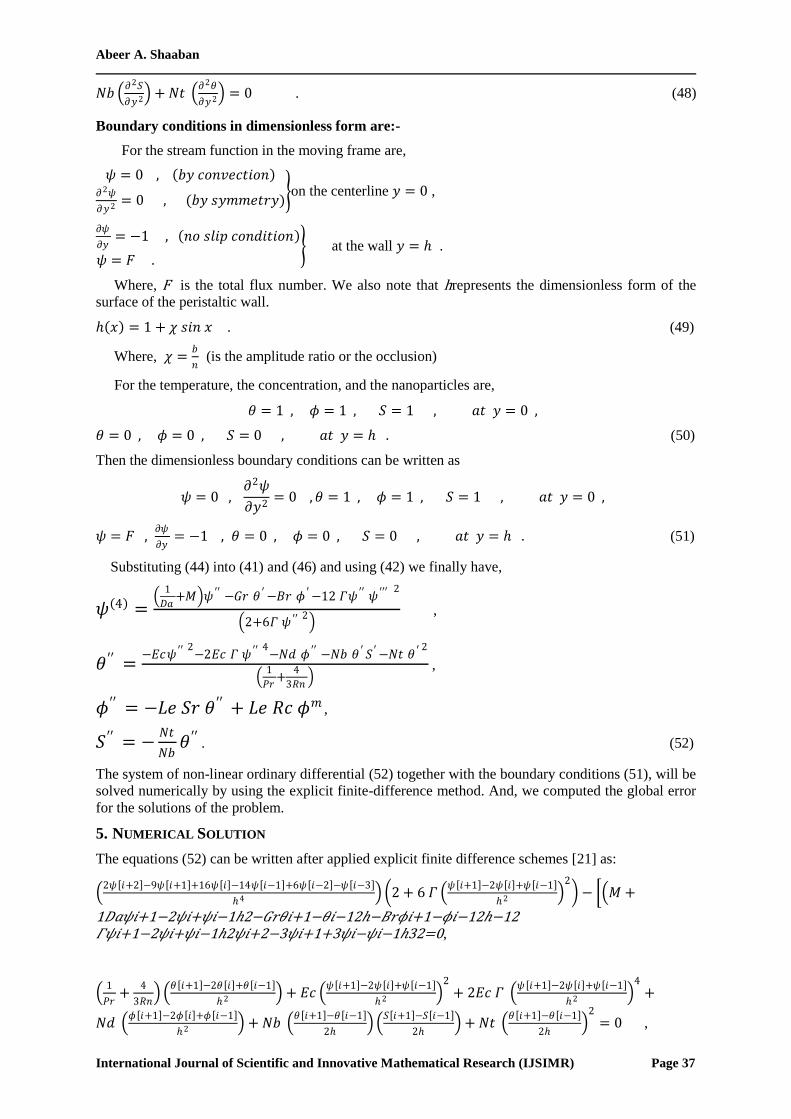
5. NUMERICAL SOLUTION

The equations (52) can be written after applied explicit finite difference schemes [21] as:

2𝜓 𝑖+2 −9𝜓 𝑖+1 +16𝜓 𝑖 −14𝜓 𝑖−1 +6𝜓 𝑖−2 −𝜓 𝑖−3

𝑕4 2 + 6 𝛤 𝜓 𝑖+1 −2𝜓 𝑖 +𝜓 𝑖−1

𝑕2 2 − 𝑀 +

1𝐷𝑎𝜓𝑖+1−2𝜓𝑖+𝜓𝑖−1𝑕2−𝐺𝑟𝜃𝑖+1−𝜃𝑖−12𝑕−𝐵𝑟𝜙𝑖+1−𝜙𝑖−12𝑕−12 𝛤𝜓𝑖+1−2𝜓𝑖+𝜓𝑖−1𝑕2𝜓𝑖+2−3𝜓𝑖+1+3𝜓𝑖−𝜓𝑖−1𝑕32=0,

1

𝑃𝑟+

4

3𝑅𝑛

𝜃 𝑖+1 −2𝜃 𝑖 +𝜃 𝑖−1

𝑕2 + 𝐸𝑐 𝜓 𝑖+1 −2𝜓 𝑖 +𝜓 𝑖−1

𝑕2 2

+ 2𝐸𝑐 𝛤 𝜓 𝑖+1 −2𝜓 𝑖 +𝜓 𝑖−1

𝑕2 4

+

𝑁𝑑 𝜙 𝑖+1 −2𝜙 𝑖 +𝜙 𝑖−1

𝑕2 + 𝑁𝑏 𝜃 𝑖+1 −𝜃 𝑖−1

2𝑕

𝑆 𝑖+1 −𝑆 𝑖−1

2𝑕 + 𝑁𝑡

𝜃 𝑖+1 −𝜃 𝑖−1

2𝑕

2= 0 ,


Chemical Reaction


𝜙 𝑖+1 −2𝜙 𝑖 +𝜙 𝑖−1

𝑕2 + 𝐿𝑒 𝑆𝑟 𝜃 𝑖+1 −2𝜃 𝑖 +𝜃 𝑖−1

𝑕2 − 𝐿𝑒 𝑅𝑐 𝜙 𝑖 𝑚 = 0 ,

𝑆 𝑖+1 −2𝑆 𝑖 +𝑆 𝑖−1

𝑕2 + 𝑁𝑡𝑁𝑏

𝜃 𝑖+1 −2𝜃 𝑖 +𝜃 𝑖−1

𝑕2 = 0 , (53)

Where the index 𝑖 refers to 𝑦 and the ∆ 𝑦 = 𝑕 = 0.04 . According to the boundary conditions (51) we

can solved equations (53) numerically, then a Newtonian iteration method continues until either of

goals specified by accuracy goal or precision goal is achieved.

6. ESTIMATION OF THE GLOBAL ERROR

We used Zadunaisky technique [22] for calculating the global error for the solutions of the problem.

We calculate an estimation of the global error from the formulas,

𝑒𝑛 = 𝑓𝑛 − 𝑓 𝑥𝑛 = 𝑓𝑛 − 𝑃 𝑥𝑛 , 𝑛 = 0,1,2,……… ,25 . (54)

In this relation, 𝑓𝑛 is the approximate solutions of the new problem (the pseudo-problem) at the point

𝑥𝑛 , and 𝑓 𝑥𝑛 is the exact solutions of pseudo-problem at 𝑥𝑛 .

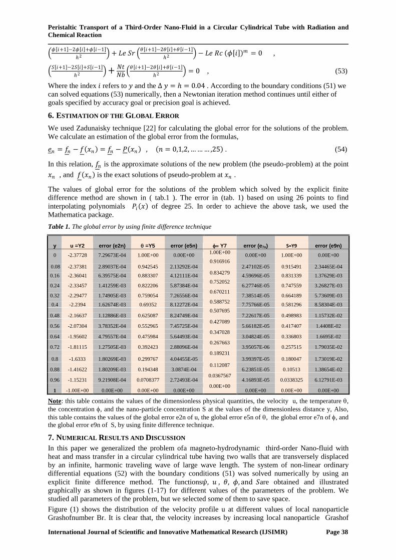
The values of global error for the solutions of the problem which solved by the explicit finite

difference method are shown in ( tab.1 ). The error in (tab. 1) based on using 26 points to find

interpolating polynomials 𝑃𝑖 𝑥 of degree 25. In order to achieve the above task, we used the

Mathematica package.

Table 1. The global error by using finite difference technique

y u =Y2 error (e2n) =Y5 error (e5n)

Y7 error (e7n) S=Y9 error (e9n)

0 -2.37728 7.29673E-04 1.00E+00 0.00E+00 1.00E+00

0.00E+00 1.00E+00 0.00E+00

0.08 -2.37381 2.89037E-04 0.942545 2.13292E-04 0.916916

2.47102E-05 0.915491 2.34465E-04

0.16 -2.36041 6.39575E-04 0.883307 4.12111E-04 0.834279

4.59696E-05 0.831339 1.37629E-03

0.24 -2.33457 1.41259E-03 0.822206 5.87384E-04 0.752052

6.27746E-05 0.747559 3.26827E-03

0.32 -2.29477 1.74905E-03 0.759054 7.26556E-04 0.670211

7.38514E-05 0.664189 5.73609E-03

0.4 -2.2394 1.62674E-03 0.69352 8.12272E-04 0.588752

7.75766E-05 0.581296 8.58304E-03

0.48 -2.16637 1.12886E-03 0.625087 8.24749E-04 0.507695

7.22617E-05 0.498983 1.15732E-02

0.56 -2.07304 3.78352E-04 0.552965 7.45725E-04 0.427089

5.66182E-05 0.417407 1.4408E-02

0.64 -1.95602 4.79557E-04 0.475984 5.64493E-04 0.347028

3.04824E-05 0.336803 1.6695E-02

0.72 -1.81115 1.27505E-03 0.392423 2.88096E-04 0.267663

3.95057E-06 0.257515 1.79035E-02

0.8 -1.6333 1.80269E-03 0.299767 4.04455E-05 0.189231

3.99397E-05 0.180047 1.73019E-02

0.88 -1.41622 1.80209E-03 0.194348 3.0874E-04 0.112087

6.23851E-05 0.10513 1.38654E-02

0.96 -1.15231 9.21908E-04 0.0708377 2.72493E-04 0.0367567

4.16893E-05 0.0338325 6.12791E-03

1 -1.00E+00 0.00E+00 0.00E+00 0.00E+00 0.00E+00

0.00E+00 0.00E+00 0.00E+00

Note: this table contains the values of the dimensionless physical quantities, the velocity u, the temperature,

the concentration , and the nano-particle concentration S at the values of the dimensionless distance y, Also,

this table contains the values of the global error e2n of u, the global error e5n of , the global error e7n of , and

the global error e9n of S, by using finite difference technique.

7. NUMERICAL RESULTS AND DISCUSSION

In this paper we generalized the problem ofa magneto-hydrodynamic third-order Nano-fluid with

heat and mass transfer in a circular cylindrical tube having two walls that are transversely displaced

by an infinite, harmonic traveling wave of large wave length. The system of non-linear ordinary

differential equations (52) with the boundary conditions (51) was solved numerically by using an

explicit finite difference method. The functions𝜓, 𝑢 , 𝜃, 𝜙, and 𝑆are obtained and illustrated

graphically as shown in figures (1-17) for different values of the parameters of the problem. We

studied all parameters of the problem, but we selected some of them to save space.

Figure (1) shows the distribution of the velocity profile u at different values of local nanoparticle

Grashofnumber Br. It is clear that, the velocity increases by increasing local nanoparticle Grashof

Abeer A. Shaaban


number Br in the region 0 ≤ 𝑦 ≤ 0.45 and, it returns decrease at 0.45 ≤ 𝑦 ≤ 1. And, we have led to

the local temperature Grashof number Greffects on the velocity the same effect of local nanoparticle

Grashofnumber Br on the velocity.

Figure (2) describes the effect of the Darcy number Da on the stream function. It is noted that, by

increasing of the Darcy number Da, the stream function decreases. And, we have led to the Darcy

number Da effects on the temperature the opposite effect of the Darcy number Da on the stream

function. Figure (3) illustrates the distributions of the velocity profile at different values of the Darcy

number Da. It is seen that, the velocity decreases by increasing the Darcy number Da in the region

0 ≤ 𝑦 ≤ 0.55 and, it returns increase at 0.55 ≤ 𝑦 ≤ 1.

-2.5

-2.3

-2.1

-1.9

-1.7

-1.5

-1.3

-1.10 0.2 0.4 0.6 0.8 1

Th

e d

imen

sio

nle

ss V

elo

cit

y u The dimensionless distance y

FIG. 1: Profiles of the velocity u(y) with various values of Br for a system have the particulars M=1.5, Da=0.1, Gr=0.1, Ec=0.5, Pr=0.7, Rn=2, Nd=2, Nb=0.5, Nt=0.1, Le=0.5, Sr=0.2, Rc=0.1, m=2.

Br=1

Br=5

Br=10

Br=20

-2.5

-2

-1.5

-1

-0.5

0

0 0.2 0.4 0.6 0.8 1

Th

e d

imen

sio

nle

ss

str

eam

fu

ncu

tio

n 𝝍

The dimensionless distance y

FIG. 2: Profiles of the stream function 𝝍(y) with various values of Da for a system have the particulars M=1.5, Gr=0.1, Br=0.1, Ec=0.5, Pr=0.7, Rn=2, Nd=2, Nb=0.5, Nt=0.1, Le=0.5, Sr=0.2, Rc=0.1, m=2.

Da=0.001

Da=0.01

Da=0.1

Da=1

-2.5

-2.3

-2.1

-1.9

-1.7

-1.5

-1.3

-1.10 0.2 0.4 0.6 0.8 1

Th

e d

imen

sio

nle

ss V

elo

cit

y u The dimensionless distance y

FIG. 3: Profiles of the velocity u(y) with various values of Da for a system have the particulars M=1.5, Gr=0.1, Br=0.1, Ec=0.5, Pr=0.7, Rn=2, Nd=2, Nb=0.5, Nt=0.1, Le=0.5, Sr=0.2, Rc=0.1, m=2.

Da=0.001

Da=0.01

Da=0.1

Da=1


Chemical Reaction


Figure (4) shows the effect of magnetic field parameter M on the stream function. It is clear that, the

stream function increases by increasing of magnetic field parameter M. And, we have led to magnetic

field parameter M effects on the temperature the opposite effect of magnetic field parameter M on the

stream function. Figure (5) illustrates the effect of magnetic field parameter M on the velocity

profiles. It is clear that, the velocity increases by increasing magnetic field parameter M in the region

0 ≤ 𝑦 ≤ 0.5 and, it returns decrease at 0.5 ≤ 𝑦 ≤ 1.

Figure (6, 7) show the effect of Eckert number Ec on the temperature, and concentration profiles,

respectively. It is seen that, the temperature increases by increasing of Eckert number Ec, but the

concentration decreases by increasing of Eckert number Ec.And, we have led to Eckert number Ec

effects on the nanoparticles the same effect of Eckert number Ec on the concentration.

-2.5

-2

-1.5

-1

-0.5

0

0 0.2 0.4 0.6 0.8 1

Th

e d

imen

sio

nle

ss s

tream

fu

ncu

tio

n 𝝍


FIG. 4: Profiles of the stream function 𝝍(y) with various values of M for a system have the particulars Da=0.1, Gr=0.1, Br=0.1, Ec=0.5, Pr=0.7, Rn=2, Nd=2, Nb=0.5, Nt=0.1, Le=0.5, Sr=0.2, Rc=0.1, m=2.

M=1.5

M=20

M=50

M=100

-2.5

-2.3

-2.1

-1.9

-1.7

-1.5

-1.3

-1.10 0.2 0.4 0.6 0.8 1

Th

e d

imen

sio

nle

ss V

elo

cit

y u


FIG. 5: Profiles of the velocity u(y) with various values of M for a system have the particulars Da=0.1, Gr=0.1, Br=0.1, Ec=0.5, Pr=0.7, Rn=2, Nd=2, Nb=0.5, Nt=0.1, Le=0.5, Sr=0.2, Rc=0.1, m=2.

M=1.5M=20

M=50M=100

0

0.2

0.4

0.6

0.8

1

1.2

0 0.2 0.4 0.6 0.8 1

Th

e d

imen

sio

nle

ss T

em

pera

ture

θ


FIG. 6: Profiles of the Temperature θ(y) with various values of Ec for a system have the particulars Da=0.1, Gr=0.1, Br=0.1, M=1.5, Pr=0.7, Rn=2, Nd=2, Nb=0.5, Nt=0.1, Le=0.5, Sr=0.2, Rc=0.1, m=2.

Ec=0.5

Ec=1

Ec=2

Ec=4

Abeer A. Shaaban


Figure (8) illustrates the effect of Dufour number Nd on the nanoparticles profiles. It is seen that, the

nanoparticles decreases by increasing of Dufour number Nd. And, we have led to Dufournumber Nd

effects on the concentration the same effect of Dufour number Nd on the nanoparticles, and the

opposite effect on the temperature.

Figure (9) obtains the effect of Brownian motion parameter Nb on the concentration profiles. It is

clear that, the concentration decreases by increasing of Brownian motion parameter Nb. And, we have

led to Brownian motion parameter Nb effects on the temperature and the nanoparticles the same effect

of Brownian motion parameter Nb on the concentration.

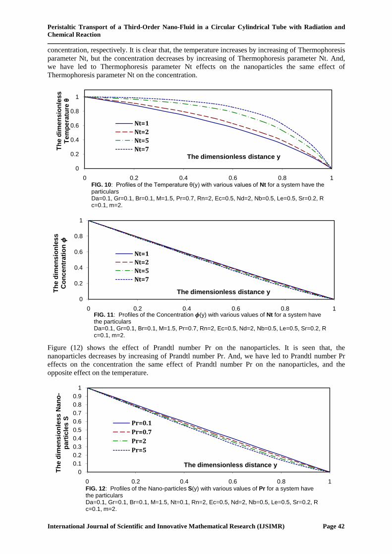
Figure (10, 11) shows the effect of Thermophoresis parameter Nt on the temperature and the

0

0.2

0.4

0.6

0.8

1

0 0.2 0.4 0.6 0.8 1

Th

e d

imen

sio

nle

ss

Co

ncen

trati

on

𝝓


FIG. 7: Profiles of the Concentration 𝝓(y) with various values of Ec for a system have the particulars Da=0.1, Gr=0.1, Br=0.1, M=1.5, Pr=0.7, Rn=2, Nd=2, Nb=0.5, Nt=0.1, Le=0.5, Sr=0.2, Rc=0.1, m=2.

Ec=0.5

Ec=1

Ec=2

Ec=4

0

0.1

0.2

0.3

0.4

0.5

0.6

0.7

0.8

0.9

1

0 0.2 0.4 0.6 0.8 1

Th

e d

imen

sio

nle

ss N

an

o-

part

icle

s S


FIG. 8: Profiles of the Nano-particles S(y) with various values of Nd for a system have the particulars Da=0.1, Gr=0.1, Br=0.1, M=1.5, Pr=0.7, Rn=2, Ec=0.5, Nb=0.5, Nt=0.1, Le=0.5, Sr=0.2, Rc=0.1, m=2.

Nd=0.1

Nd=5

Nd=10

Nd=15

0

0.2

0.4

0.6

0.8

1

0 0.2 0.4 0.6 0.8 1

Th

e d

imen

sio

nle

ss

Co

ncen

trati

on

𝝓


FIG. 9: Profiles of the Concentration 𝝓(y) with various values of Nb for a system have the particulars Da=0.1, Gr=0.1, Br=0.1, M=1.5, Pr=0.7, Rn=2, Ec=0.5, Nd=2, Nt=0.1, Le=0.5, Sr=0.2, Rc=0.1, m=2.

Nb=0.1

Nb=1.5

Nb=5

Nb=10


Chemical Reaction


concentration, respectively. It is clear that, the temperature increases by increasing of Thermophoresis

parameter Nt, but the concentration decreases by increasing of Thermophoresis parameter Nt. And,

we have led to Thermophoresis parameter Nt effects on the nanoparticles the same effect of

Thermophoresis parameter Nt on the concentration.

Figure (12) shows the effect of Prandtl number Pr on the nanoparticles. It is seen that, the

nanoparticles decreases by increasing of Prandtl number Pr. And, we have led to Prandtl number Pr

effects on the concentration the same effect of Prandtl number Pr on the nanoparticles, and the


0

0.2

0.4

0.6

0.8

1

0 0.2 0.4 0.6 0.8 1

Th

e d

imen

sio

nle

ss

Tem

pera

ture

θ


FIG. 10: Profiles of the Temperature θ(y) with various values of Nt for a system have the particulars Da=0.1, Gr=0.1, Br=0.1, M=1.5, Pr=0.7, Rn=2, Ec=0.5, Nd=2, Nb=0.5, Le=0.5, Sr=0.2, Rc=0.1, m=2.

Nt=1

Nt=2

Nt=5

Nt=7

0

0.2

0.4

0.6

0.8

1

0 0.2 0.4 0.6 0.8 1

Th

e d

imen

sio

nle

ss

Co

ncen

trati

on

𝝓


FIG. 11: Profiles of the Concentration 𝝓(y) with various values of Nt for a system have the particulars Da=0.1, Gr=0.1, Br=0.1, M=1.5, Pr=0.7, Rn=2, Ec=0.5, Nd=2, Nb=0.5, Le=0.5, Sr=0.2, Rc=0.1, m=2.

Nt=1

Nt=2

Nt=5

Nt=7

0

0.1

0.2

0.3

0.4

0.5

0.6

0.7

0.8

0.9

1

0 0.2 0.4 0.6 0.8 1

Th

e d

imen

sio

nle

ss N

an

o-

part

icle

s S


FIG. 12: Profiles of the Nano-particles S(y) with various values of Pr for a system have the particulars Da=0.1, Gr=0.1, Br=0.1, M=1.5, Nt=0.1, Rn=2, Ec=0.5, Nd=2, Nb=0.5, Le=0.5, Sr=0.2, Rc=0.1, m=2.

Pr=0.1

Pr=0.7

Pr=2

Pr=5

Abeer A. Shaaban


Figure (13, 14) illustrate the effect of radiation parameter Rnon the temperature and nanoparticles,

respectively. It is shown that, the temperature increases by increasing of radiation parameter Rn, but

the nanoparticles decreases by increasing of radiation parameter Rn. And, we have led to radiation

parameter Rn effects on the concentration the same effect of radiation parameter Rn on the

nanoparticles.

Figure (15) shows the effect of Lewis number Le on the concentration. It is clear that, the

concentration decreases by increasing of Lewis number Le. And, we have led to Lewis number Le

effects on the nanoparticles the same effect of Lewis number Le on the concentration, and the


0

0.2

0.4

0.6

0.8

1

0 0.2 0.4 0.6 0.8 1

Th

e d

imen

sio

nle

ss

Tem

pera

ture

θ


FIG. 13: Profiles of the Temperature θ(y) with various values of Rn for a system have the particulars Da=0.1, Gr=0.1, Br=0.1, M=1.5, Nt=0.1, Pr=0.7, Ec=0.5, Nd=2, Nb=0.5, Le=0.5, Sr=0.2, Rc=0.1, m=2.

Rn=0.01

Rn=1

Rn=2

Rn=50

0

0.1

0.2

0.3

0.4

0.5

0.6

0.7

0.8

0.9

1

0 0.2 0.4 0.6 0.8 1

Th

e d

imen

sio

nle

ss N

an

o-

part

icle

s S


FIG. 14: Profiles of the Nano-particles S(y) with various values of Rn for a system have the particulars Da=0.1, Gr=0.1, Br=0.1, M=1.5, Nt=0.1, Pr=0.7, Ec=0.5, Nd=2, Nb=0.5, Le=0.5, Sr=0.2, Rc=0.1, m=2.

Rn=0.01

Rn=1

Rn=2

Rn=50

-0.1

0.1

0.3

0.5

0.7

0.9

0 0.2 0.4 0.6 0.8 1

Th

e d

imen

sio

nle

ss

Co

ncen

trati

on

𝝓


FIG. 15: Profiles of the Concentration 𝝓(y) with various values of Le for a system have the particulars Da=0.1, Gr=0.1, Br=0.1, M=1.5, Nt=0.1, Pr=0.7, Ec=0.5, Nd=2, Nb=0.5, Rn=2, Sr=0.2, Rc=0.1, m=2.

Le=0.01

Le=1

Le=2

Le=3


Chemical Reaction


Figure (16) shows the effect of Sort number Sr on the nanoparticles. It is seen that, the nanoparticles

decreases by increasing of Sort number Sr. And, we have led to Sort number Sr effects on the

concentration the same effect Sort number Sr on the nanoparticles, and the opposite effect on the

temperature.

Figure (17) shows the effect of Chemical reaction parameter Rc on the concentration. It is clear that,

the concentration decreases by increasing of Chemical reaction parameter Rc. And, we have led to

Chemical reaction parameter Rc effects on the nanoparticles the same effect of Chemical reaction

parameter Rc on the concentration, and the opposite effect on the temperature.

8. CONCLUSION

In this work, we have studied a magneto-hydrodynamic third-order Nano-fluid with heat and mass

transfer in a circular cylindrical tube having two walls that are transversely displaced by an infinite,

harmonic traveling wave of large wave length. The governing boundary value problem was solved

numerically by an Explicit Finite-Difference method. We concentrated our work on obtaining the

stream function, the velocity, the temperature, the concentration, and the nanoparticlesdistributions

which are illustrated graphically at different values of the parameters of the problem. Global error

estimation is also obtained using Zadunaisky technique. We used 26 points to find the interpolating

polynomial of degree 25 in interval [0,1] and the results are shown in ( tab.1 ). We notice that, the

error in ( tab.1) is good enough to justify the use of resulting numerical values.

0

0.1

0.2

0.3

0.4

0.5

0.6

0.7

0.8

0.9

1

0 0.2 0.4 0.6 0.8 1

Th

e d

ime

nsio

nle

ss N

an

o-p

art

icle

s S


FIG. 16: Profiles of the Nano-particles S(y) with various values of Sr for a system have the particulars Da=0.1, Gr=0.1, Br=0.1, M=1.5, Nt=0.1, Pr=0.7, Ec=0.5, Nd=2, Nb=0.5, Rn=2, Le=0.5, Rc=0.1, m=2.

Sr=3

Sr=3.5

Sr=4.5

Sr=7

-0.2

0

0.2

0.4

0.6

0.8

1

0 0.2 0.4 0.6 0.8 1

Th

e d

imen

sio

nle

ss C

on

cen

trati

on

𝝓


FIG. 17: Profiles of the Concentration 𝝓(y) with various values of Rc for a system have the particulars Da=0.1, Gr=0.1, Br=0.1, M=1.5, Nt=0.1, Pr=0.7, Ec=0.5, Nd=2, Nb=0.5, Rn=2, Le=0.5, Sr=0.2, m=2.

Rc=0.1

Rc=2

Rc=5

Rc=10

Abeer A. Shaaban


REFERENCES

[1] HayatT. and AliN., Peristaltically induced motion of a MHD third grade fluid in a deformable

tube, Physica A. 370, 225, (2006).

[2] Latham T. W., Fluids Motions in a Peristaltic Pump, Thesis, M. I. T., Cambridge, (1966).

[3] HarounM. H., Effect of Deborah Number and Phase Difference on Peristaltic transport of a

Third-Order Fluid in an Asymmetric Channel, Communication in Nonlinear Science and

Numerical Simulation.12, 1464, (2007).

[4] EldabeN. T. M., El-SayedM. F., GhalyA. Y. and SayedH. M., Peristaltically Induced Transport

of a MHD Biviscosity Fluid in a Non-Uniform Tube, Physica A. 383, 253, (2007).

[5] HayatT., AfsarA., KhanM.and AsgharS.,Peristaltic transport of a third order fluid under the

effect of a magnetic field, Computers and Mathematics with Applications. 53, 1074, (2007).

[6] EllahiR., RazaM. and VafaiK.,Series solutions of non-Newtonian nanofluids with Reynolds’

model and Vogel’s model by means of the homotopy analysis method, Mathematical and

Computer Modelling. 55, 1876, (2012).

[7] ChoiS. U., Enhancing thermal conductivity of fluids with nanoparticle, ASME J. Develop.

[8] Appl. Non-Newtonian Flows. 66, 99, (1995).

[9] FarooqU., HayatT., AlsaediA.and LiaoShijun, Heat and mass transfer of two-layer flows of

third-grade nano-fluids in a vertical channel, Applied Mathematics and Computation. 242, 528,

(2014).

[10] TzirtzilakisE. E., A mathematical model for blood flow in magnetic field, Physics of Fluids.

17,077103, (2005).

[11] BakierA. Y., Thermal radiation effect on mixed convection from vertical surface in saturated

porous media, International Journal of Communication of Heat and Mass Transfer.28, 119,

(2001).

[12] DamsehR. A., Magnetohydrodynamics-mixed convection from radiate vertical isothermal

surface embedded in a saturated porous media, Journal of Applied Mechanics. 73, 54, (2006).

[13] HossainM. A. and TakharH. S., Radiation effect on mixed convection along a vertical plate with

uniform surface temperature, Heat and Mass Transfer. 31, 243, (1996).

[14] ZahmatkeshI., Influence of thermal radiation on free convection inside a porous enclosure,

Emirates Journal for Engineering Research. 12, 47, (2007).

[15] SheikholeslamiMohsen, DomiriGanjiDavood, YounusJavedM. and EllahiR., Effect of thermal

radiation on magnetohydrodynamicsnanofluids flow and heat transfer by means of two phase

model, Journal of Magnetism and Magnetic Materials. 374, 36, (2015).

[16] HinaS., HayatT., AsgharS. and HendiAwatif A., Influence of compliant walls on peristaltic

motion with heat/mass transfer and chemical reaction, International Journal of Heat and Mass

Transfer. 55, 3386, (2012).

[17] VajraveluK., PrasadK. V.and AbbasbandyS., Convection transport of nanoparticle in multi-layer

fluid flow, Appl. Math. Mech. Eng. Ed.34(2), 177 (2013).

[18] FarooqU., HayatT., AlsaediA. and LiaoShijun, Heat and mass transfer of two-layer flows of

third-grade nano-fluids in a vertical channel, Appl. Math. Comp. 242, 528, (2014).

[19] Abou-zeidMohamed Y., ShaabanAbeer A. and AlnourMuneer Y., Numerical treatment and

global error estimation of natural convective effects on gliding motion of bacteria on a power-

law nanoslime through a non-Darcy porous medium, J. Porous Media. 18(11), 1091,(2015).

[20] El-dabeNabil T.M., ShaabanAbeer A., Abou-zeidMohamed Y.and AliHemat A., MHD non-

Newtonian nanofluid flow over a stretching sheet with thermal diffusion and diffusion thermo

effects through a non-Darcy porous medium with radiation and chemical reaction, J. Compu.

Theor. Nanoscience. 12(11), 5363, ( 2015).

[21] ShaabanA. A. and Abou-zeidM. Y., Effects of Heat and Mass Transfer on MHD Peristaltic Flow

of a Non-Newtonian Fluid through a Porous Medium between Two Coaxial Cylinders,

Mathematical Problems in Engineering, 2013, 1, (2013).

[22] ZadunaiskyP. E., On the Estimation of Errors Propagated in the Numerical Integration of

Ordinary Differential Equations, Numerical Mathematics.27,21, (1976).


Chemical Reaction


[23] FosdickR. L. and RajagopalK. R., Thermodynamics and stability of fluids of third-grade, Proc.

Roy. Soc. London A. 339, 351, (1980).

[24] DunnJ. E. and RajagopalK. R., Fluids of differential type-critical-review and thermos dynamic

analysis, Int. J. Eng. Sci. 33, 689, (1995).

[25] EldabeN. T. M., HassanA. A.and MohamedM. A. A., Effect of couple stresses on the MHD of a

non-Newtonian unsteady flow between two parallel porous plates, Z. Naturforsch. 58 a, 204,

(2003).

[26] EldabeN. T. M.and MohamedM. A. A., Heat and mass transfer in Hydromagnetic flow of the

non-Newtonian fluid with heat source over an accelerating surface through a porous medium,

Chaos, Solitons and Fractals. 13, 907, (2002).

[27] C. P. Arora, Heat and Mass transfer, Khanna Publishers Delhi, (1997).

[28] RaptisA., Flow of a micropolar fluid past a continuously moving plate by presence of radiation,

Int. J. Heat and Mass Transfer. 41, 2865, (1998).

[29] ShapiroA. H., JaffrinM. Y. and WeinbergS. L., Peristaltic pumping with long wavelengths at low

Reynolds number, J. Fluid Mech. 37, 799, (1969).

Peristaltic Transport of a Third-Order Nano-Fluid in a ... · Peristaltic Transport of a...

Documents

Transcript of Peristaltic Transport of a Third-Order Nano-Fluid in a ... · Peristaltic Transport of a...