Digital Object Identifier (DOI) 10.1007/s00220-004-1255-8Commun. Math. Phys. 256, 437–490 (2005) Communications in

MathematicalPhysics

Periodic Solutions for Completely Resonant NonlinearWave Equations with Dirichlet Boundary Conditions

Guido Gentile1, Vieri Mastropietro2, Michela Procesi3

1 Dipartimento di Matematica, Universita di Roma Tre, 00146 Roma, Italy2 Dipartimento di Matematica, Universita di Roma “Tor Vergata”, 00133 Roma, Italy3 SISSA, 34014 Trieste, Italy

Received: 24 February 2004 / Accepted: 26 May 2004Published online: 4 February 2005 – © Springer-Verlag 2005

Abstract: We consider the nonlinear string equation with Dirichlet boundary conditionsutt −uxx = ϕ(u), with ϕ(u) = �u3 +O(u5) odd and analytic, � �= 0, and we constructsmall amplitude periodic solutions with frequency ω for a large Lebesgue measure set ofω close to 1. This extends previous results where only a zero-measure set of frequenciescould be treated (the ones for which no small divisors appear). The proof is based oncombining the Lyapunov-Schmidt decomposition, which leads to two separate sets ofequations dealing with the resonant and non-resonant Fourier components, respectivelythe Q and the P equations, with resummation techniques of divergent powers series,allowing us to control the small divisors problem. The main difficulty with respect tothe nonlinear wave equations utt − uxx + Mu = ϕ(u), M �= 0, is that not only the Pequation but also the Q equation is infinite-dimensional.

1. Introduction

We consider the nonlinear wave equation in d = 1 given by{

utt − uxx = ϕ(u),

u(0, t) = u(π, t) = 0,(1.1)

where Dirichlet boundary conditions allow us to use as a basis in L2([0, π ]) the set offunctions {sin mx, m ∈ N}, and ϕ(u) is any odd analytic function ϕ(u) = �u3 +O(u5)

with � �= 0. We shall consider the problem of existence of periodic solutions for (1.1),which represents a completely resonant case for the nonlinear wave equation as in theabsence of nonlinearities all the frequencies are resonant.

In the finite dimensional case the problem has its analogue in the study of periodicorbits close to elliptic equilibrium points: results of existence have been obtained in sucha case by Lyapunov [31] in the non-resonant case, by Birkhoff and Lewis [6] in the caseof resonances of order greater than four, and by Weinstein [37] in the case of any kind

438 G. Gentile, V. Mastropietro, M. Procesi

of resonances. Systems with infinitely many degrees of freedom (as the nonlinear waveequation, the nonlinear Schrodinger equation and other PDE systems) have been studiedmuch more recently; the problem is much more difficult because of the presence of asmall divisors problem, which is absent in the finite dimensional case. For the nonlinearwave equations utt −uxx +Mu = ϕ(u), with mass M strictly positive, existence of peri-odic solutions has been proved by Craig and Wayne [14], by Poschel [33] (by adaptingthe analogous result found by Kuksin and Poschel [29] for the nonlinear Schrodingerequation) and by Bourgain [8] (see also the review [13]). In order to solve the small divi-sors problem one has to require that the amplitude and frequency of the solution mustbelong to a Cantor set, and the main difficulty is to prove that such a set can be chosenwith non-zero Lebesgue measure. We recall that for such systems also quasi-periodicsolutions have been proved to exist in [29, 33, 9] (in many other papers the case in whichthe coefficient M of the linear term is replaced by a function depending on parametersis considered; see for instance [36, 7] and the reviews [27, 28]).

In all the quoted papers only non-resonant cases are considered. Some cases withsome low-order resonances between the frequencies have been studied by Craig andWayne [15]. The completely resonant case (1.1) has been originally studied with varia-tional methods starting from Rabinowitz [34, 35, 12, 11, 17], where periodic solutionswith a period which is a rational multiple of π have been obtained; such solutions corre-spond to a zero-measure set of values of the amplitudes. The case of irrational periods,which in principle could provide a large measure of values, has been mostly studied onlyunder strong Diophantine conditions (as the ones introduced in [2]) which essentiallyremove the small divisors problem, leaving in fact again a zero-measure set of values[30, 3, 4]. It is however conjectured that also for M = 0 periodic solutions of (1.1)should exist for a large measure set of values of the amplitudes, see for instance [28],and indeed we prove in this paper that this is actually the case: the unperturbed periodicsolutions with periods Tj = 2π/j can be continued into periodic solutions with periodsTε,j = 2π/j

√1 − ε, where ε is a small parameter of the order of the squared amplitude

of the periodic solution.In [10] existence of periodic solutions is proved for the equation utt − uxx = u3 +

F(x, u), with periodic boundary conditions, and with F(x, u) a polynomial in u withcoefficients which are trigonometric polynomials in x. Such a problem becomes triv-ial when F does not depend explicitly on x (in [10] Wayne is credited with such anobservation), for instance if F(x, u) ≡ 0. On the other hand, when a function F(x, u)

depending on x is considered, the perturbation of the exactly solvable problem appearsto order higher than 1 (in ε), and this produces a small divisor problem which is solvedby imposing a Diophantine condition with an ε-dependent constant (see (5.35) in [10]).

On the contrary in the case of Dirichlet boundary conditions to find a periodic solu-tion just for the cubic equation, utt − uxx = u3, is non-trivial, and, as will be apparentlater on, it is essentially the core of the problem. It already requires the solution of asmall divisor problem: one considers the term u3 as a perturbation and the problem iscomplicated by the fact that utt − uxx can be of the same order of u3; in particular wemust impose a Diophantine condition with an ε-independent constant, and this requirescareful control of the small divisors.

Of course the techniques used in our and Bourgain’s papers are quite different. Bour-gain uses the Craig-Wayne approach based on the method of Frohlich and Spencer [18],while we rely on the Renormalization Group approach proposed in [23], which consistsof a Lyapunov-Schmidt decomposition followed by a tree expansion of the solution (witha graphic formalism originally introduced by Gallavotti [19], inspired by Eliasson’s work

Nonlinear Wave Equations with Dirichlet Boundary Conditions 439

[16], for investigating the persistence of maximal KAM tori), which allows us to controlthe small divisors problem. As in [3] and [5] we also consider the problem of findinghow many solutions can be obtained with a given period, and we study their minimalperiod. As a further minor difference between the present paper and [10], we mentionthat our solutions are analytic in space and time, while the ones found by Bourgain areC∞.

If ϕ = 0 every real solution of (1.1) can be written as

u(x, t) =∞∑

n=1

Un sin nx cos(ωnt + θn), (1.2)

where ωn = n and Un ∈ R for all n ∈ N.For ε > 0 we set � = σF , with σ = sgn� and F > 0, and rescale u → √

ε/Fu in(1.1), thus obtaining {

utt − uxx = σεu3 + O(ε2),

u(0, t) = u(π, t) = 0,(1.3)

where O(ε2) denotes an analytic function of u and ε of order at least 2 in ε, and wedefine ωε = √

1 − λε, with λ ∈ R, so that ωε = 1 for ε = 0.As the nonlinearity ϕ is odd the solution of (1.3) can be extended in the x variable to

an odd 2π -periodic function (even in the variable t). We shall consider ε small and weshall show that there exists a solution of (1.3), which is 2π/ωε-periodic in t and ε-closeto the function

u0(x, ωεt) = a0(ωεt + x) − a0(ωεt − x), (1.4)

provided that ε is in an appropriate Cantor set and a0(ξ) is the odd 2π -periodic solutionof the integro-differential equation

σλa0 = −3⟨a2

0

⟩a0 − a3

0, (1.5)

where the dot denotes the derivative with respect to ξ , and, given any periodic functionF(ξ) with period T , we denote by

〈F 〉 = 1

T

∫ T

0dξ F (ξ) (1.6)

its average. Then a 2π/ωε-periodic solution of (1.1) is simply obtained by scaling backthe solution of (1.3).

Equation (1.5) has odd 2π -periodic solutions, provided that one sets σλ > 0; weshall choose σλ = 1 in the following. An explicit computation gives [3]

a0(ξ) = Vm sn(mξ, m) (1.7)

for m a suitable negative constant (m ≈ −0.2554), with m = 2K(m)/π and Vm =√−2mm, where sn(mξ, m) is the sine-amplitude function and K(m) is the ellipticintegral of the first kind, with modulus

√m [25]; see Appendix A1 for further details.

Call 2κ the width of the analyticity strip of the function a0(ξ) and α the maximum valueit can assume in such a strip; then one has∣∣a0,n

∣∣ ≤ αe−2k|n|. (1.8)

440 G. Gentile, V. Mastropietro, M. Procesi

Our result (including also the cases of frequencies which are multiples of ωε) can bemore precisely stated as follows.

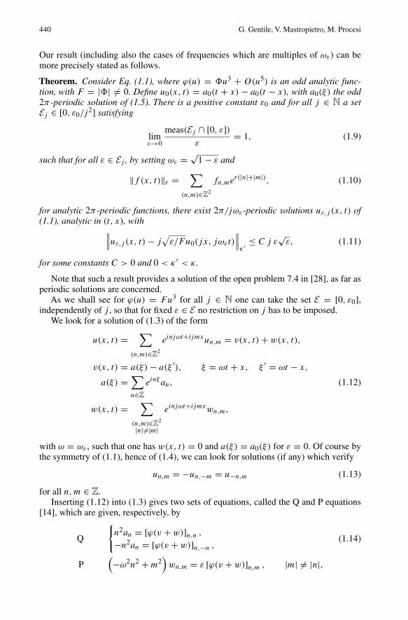
Theorem. Consider Eq. (1.1), where ϕ(u) = �u3 + O(u5) is an odd analytic func-tion, with F = |�| �= 0. Define u0(x, t) = a0(t + x) − a0(t − x), with a0(ξ) the odd2π -periodic solution of (1.5). There is a positive constant ε0 and for all j ∈ N a setEj ∈ [0, ε0/j

2] satisfying

limε→0

meas(Ej ∩ [0, ε])

ε= 1, (1.9)

such that for all ε ∈ Ej , by setting ωε = √1 − ε and

‖f (x, t)‖r =∑

(n,m)∈Z2

fn,mer(|n|+|m|), (1.10)

for analytic 2π -periodic functions, there exist 2π/jωε-periodic solutions uε,j (x, t) of(1.1), analytic in (t, x), with∥∥∥uε,j (x, t) − j

√ε/Fu0(jx, jωεt)

∥∥∥κ ′ ≤ C j ε

√ε, (1.11)

for some constants C > 0 and 0 < κ ′ < κ .

Note that such a result provides a solution of the open problem 7.4 in [28], as far asperiodic solutions are concerned.

As we shall see for ϕ(u) = Fu3 for all j ∈ N one can take the set E = [0, ε0],independently of j , so that for fixed ε ∈ E no restriction on j has to be imposed.

We look for a solution of (1.3) of the form

u(x, t) =∑

(n,m)∈Z2

einjωt+ijmxun,m = v(x, t) + w(x, t),

v(x, t) = a(ξ) − a(ξ ′), ξ = ωt + x, ξ ′ = ωt − x,

a(ξ) =∑n∈Z

einξ an, (1.12)

w(x, t) =∑

(n,m)∈Z2

|n|�=|m|

einjωt+ijmxwn,m,

with ω = ωε, such that one has w(x, t) = 0 and a(ξ) = a0(ξ) for ε = 0. Of course bythe symmetry of (1.1), hence of (1.4), we can look for solutions (if any) which verify

un,m = −un,−m = u−n,m (1.13)

for all n, m ∈ Z.Inserting (1.12) into (1.3) gives two sets of equations, called the Q and P equations

[14], which are given, respectively, by

Q

{n2an = [ϕ(v + w)]n,n ,

−n2an = [ϕ(v + w)]n,−n ,(1.14)

P(−ω2n2 + m2

)wn,m = ε [ϕ(v + w)]n,m , |m| �= |n|,

Nonlinear Wave Equations with Dirichlet Boundary Conditions 441

where we denote by [F ]n,m the Fourier component of the function F(x, t) with labels(n, m), so that

F(x, t) =∑

(n,m)∈Z2

einωt+mx[F ]n,m. (1.15)

In the same way we shall call [F ]n the Fourier component of the function F(ξ) withlabel n; in particular one has [F ]0 = 〈F 〉. Note also that the two equations Q are infact the same, by the symmetry property [ϕ(v + w)]n,m = − [ϕ(v + w)]n,−m, whichfollows from (1.13).

We start by considering the case ϕ(u) = u3 and j = 1, for simplicity. We shalldiscuss at the end how the other cases can be dealt with, see Sect. 8.

2. Lindstedt Series Expansion

One could try to write a power series expansion in ε for u(x, t), using (1.14) to get recur-sive equations for the coefficients. However by proceeding in this way one finds that thecoefficient of order k is given by a sum of terms some of which are of order O(k!α),for some constant α. This is the same phenomenon occurring in the Lindstedt series forinvariant KAM tori in the case of quasi-integrable Hamiltonian systems; in such a casehowever one can show that there are cancellations between the terms contributing to thecoefficient of order k, which at the end admits a bound Ck , for a suitable constant C. Onthe contrary such cancellations are absent in the present case and we have to proceedin a different way, equivalent to a resummation (see [23] where such a procedure wasapplied to the same nonlinear wave equation with a mass term, utt −uxx +Mu = ϕ(u)).

Definition 1. Given a sequence {νm(ε)}|m|≥1, such that νm = ν−m, we define the ren-ormalized frequencies as

ω2m ≡ ω2

m + νm, ωm = |m|, (2.1)

and the quantities νm will be called the counterterms.

By the above definition and the parity properties (1.13) the P equation in (1.14) canbe rewritten as

wn,m

(−ω2n2 + ω2

m

)= νmwn,m + ε[ϕ(v + w)]n,m

= ν(a)m wn,m + ν(b)

m wn,−m + ε[ϕ(v + w)]n,m, (2.2)

where

ν(a)m − ν(b)

m = νm. (2.3)

With the notations of (1.15), and recalling that we are considering ϕ(u) = u3, wecan write [

(v + w)3]n,n

= [v3]n,n + [w3]n,n + 3[v2w]n,n + 3[w2v]n,n

≡ [v3]n,n + [g(v, w)]n,n, (2.4)

442 G. Gentile, V. Mastropietro, M. Procesi

where, again by using the parity properties (1.13),

[v3]n,n = [a3]n + 3⟨a2⟩an. (2.5)

Then the first Q equation in (1.13) can be rewritten as

n2an = [a3]n + 3⟨a2⟩an + [g(v, w)]n,n , (2.6)

so that an is the Fourier coefficient of the 2π -periodic solution of the equation

a = −(a3 + 3

⟨a2⟩a + G(v, w)

), (2.7)

where we have introduced the function

G(v, w) =∑n∈Z

einξ [g(v, w)]n,n . (2.8)

To study Eqs. (2.2) and (2.6) we introduce an auxiliary parameter µ, which at the endwill be set equal to 1, by writing (2.2) as

wn,m

(−ω2n2 + ω2

m

)= µν(a)

m wn,m + µν(b)m wn,−m + µε[ϕ(v + w)]n,m, (2.9)

and we shall look for un,m in the form of a power series expansion in µ,

un,m =∞∑

k=0

µku(k)n,m, (2.10)

with u(k)n,m depending on ε and on the parameters ν

(c)

m′ , with c = a, b and |m′| ≥ 1.

In (2.10) k = 0 requires u(0)n,±n = ±a0,n and u

(0)n,m = 0 for |n| �= |m|, for k ≥ 1, as

we shall see later on, the dependence on the parameters ν(c′)m′ will be polynomial, of the

form

∞∏m′=2

∏c′=a,b

(ν

(c′)m′)k

(c′)m′

, (2.11)

with |k| = k(a)1 + k

(b)1 + k

(a)2 + k

(b)2 +· · · ≤ k − 1. Of course we are using the symmetry

property to restrict the dependence only on the positive labels m′.We derive recursive equations for the coefficients u

(k)n,m of the expansion. We start

from the coefficients with |n| = |m|.By (1.12) and (2.10) we can write

a = a0 +∞∑

k=1

µkA(k), (2.12)

and inserting this expression into (2.7) we obtain for A(k) the equation

A(k) = −3(a2

0A(k) +⟨a2

0

⟩A(k) + 2

⟨a0A

(k)⟩a0

)+ f (k), (2.13)

Nonlinear Wave Equations with Dirichlet Boundary Conditions 443

with

f (k) = −∑

k1+k2+k3=kki=k→|ni |�=|mi |

∑n1+n2+n3=n

m1+m2+m3=m

u(k1)n1,m1

u(k2)n2,m2

u(k3)n3,m3

, (2.14)

where we have used the notations

u(k)n,m =

{v

(k)n,m, if |n| = |m|,

w(k)n,m, if |n| �= |m|, (2.15)

with

v(k)n,n =

{A

(k)n , if k �= 0,

a0,n, if k = 0,v

(k)n,−n =

{−A

(k)n , if k �= 0,

−a0,n, if k = 0.(2.16)

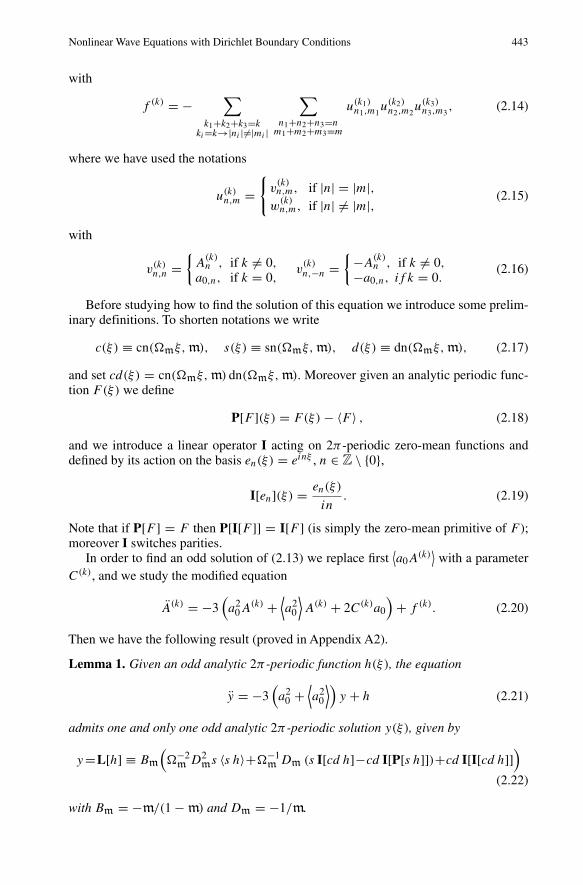
Before studying how to find the solution of this equation we introduce some prelim-inary definitions. To shorten notations we write

c(ξ) ≡ cn(mξ, m), s(ξ) ≡ sn(mξ, m), d(ξ) ≡ dn(mξ, m), (2.17)

and set cd(ξ) = cn(mξ, m) dn(mξ, m). Moreover given an analytic periodic func-tion F(ξ) we define

P[F ](ξ) = F(ξ) − 〈F 〉 , (2.18)

and we introduce a linear operator I acting on 2π -periodic zero-mean functions anddefined by its action on the basis en(ξ) = einξ , n ∈ Z \ {0},

I[en](ξ) = en(ξ)

in. (2.19)

Note that if P[F ] = F then P[I[F ]] = I[F ] (is simply the zero-mean primitive of F );moreover I switches parities.

In order to find an odd solution of (2.13) we replace first⟨a0A

(k)⟩

with a parameterC(k), and we study the modified equation

A(k) = −3(a2

0A(k) +⟨a2

0

⟩A(k) + 2C(k)a0

)+ f (k). (2.20)

Then we have the following result (proved in Appendix A2).

Lemma 1. Given an odd analytic 2π -periodic function h(ξ), the equation

y = −3(a2

0 +⟨a2

0

⟩)y + h (2.21)

admits one and only one odd analytic 2π -periodic solution y(ξ), given by

y =L[h] ≡ Bm

(−2

m D2ms 〈s h〉+−1

m Dm (s I[cd h]−cd I[P[s h]])+cd I[I[cd h]])

(2.22)

with Bm = −m/(1 − m) and Dm = −1/m.

444 G. Gentile, V. Mastropietro, M. Procesi

As a0 is analytic and odd, we find immediately, by induction on k and using Lemma1, that f (k) is analytic and odd, and that the solution of Eq. (2.20) is odd and given by

A(k) = L[−6C(k)a0 + f (k)]. (2.23)

The function A(k) thus found depends of course on the parameter C(k); in order toobtain A(k) = A(k), we have to impose the constraint

C(k) =⟨a0A

(k)⟩, (2.24)

and by (2.23) this gives

C(k) = −6C(k) 〈a0L[a0]〉 +⟨a0L[f (k)]

⟩, (2.25)

which can be rewritten as

(1 + 6 〈a0L[a0]〉) C(k) =⟨a0L[f (k)]

⟩. (2.26)

An explicit computation (see Appendix A3) gives

〈a0L[a0]〉 = 1

2V 2

m−2m Bm

((2Dm − 1

2

)〈s4〉 +

(2Dm (Dm − 1) + 1

2

)〈s2〉2

),

(2.27)

which yields r0 = (1 + 6〈a0L[a0]〉) �= 0. At the end we obtain the recursive definition

A(k) = L[f (k) − 6C(k)a0],

C(k) = r−10

⟨a0L[f (k)]

⟩.

(2.28)

In Fourier space the first of (2.28) becomes

A(k)n = Bm−2

m D2msn

∑n1+n2=0

sn1

(f (k)

n2− 6C(k)a0,n2

)

+Bm

∑n1+n2+n3=n

∗ 1

i2(n2 + n3)2 cdn1cdn2

(f (k)

n3− 6C(k)a0,n3

)

+Bm−1m Dm

∑n1+n2+n3=n

∗ 1

i(n2 + n3)sn1cdn2

(f (k)

n3− 6C(k)a0,n3

)(2.29)

−Bm−1m Dm

∑n1+n2+n3=n

∗ 1

i(n2 + n3)cdn1sn2

(f (k)

n3− 6C(k)a0,n3

)

≡∑n′

Lnn′(f

(k)

n′ − 6C(k)a0,n′)

,

where the constants Bm and Dm are defined after (2.22), and the ∗ in the sums meansthat one has the constraint n2 + n3 �= 0, while the second of (2.28) can be written as

C(k) = r−10

∑n,n′∈Z

a0,−nLn,n′f (k)

n′ . (2.30)

Nonlinear Wave Equations with Dirichlet Boundary Conditions 445

Now we consider the coefficients u(k)n,m with |n| �= |m|. The coefficients w

(k)n,m verify

the recursive equations

w(k)n,m

[−ω2n2 + ω2

m

]= ν(a)

m w(k−1)n,m + ν(b)

m w(k−1)n,−m + [(v + w)3](k−1)

n,m , (2.31)

where

[(v + w)3](k)n,m =

∑k1+k2+k3=k

∑n1+n2+n3=n

m1+m2+m3=m

u(k1)n1,m1

u(k2)n2,m2

u(k3)n3,m3

, (2.32)

if we use the same notations (2.15) and (2.16) as in (2.14).Equations (2.29) and (2.31), together with (2.32), (2.14), (2.30) and (2.32), define

recursively the coefficients u(k)n,m.

To prove the theorem we shall proceed in two steps. The first step consists in lookingfor the solution of Eqs. (2.29) and (2.31) by considering ω = {ωm}|m|≥1 as a given setof parameters satisfying the Diophantine conditions (called respectively the first and thesecond Mel′nikov conditions)

|ωn ± ωm| ≥ C0|n|−τ ∀n ∈ Z \ {0} and ∀m ∈ Z \ {0} such that |m| �= |n|,|ωn ± (ωm ± ωm′)| ≥ C0|n|−τ (2.33)

∀n ∈ Z \ {0} and ∀m, m′ ∈ Z \ {0} such that |n| �= |m ± m′|,with positive constants C0, τ . We shall prove in Sect. 3 to 5 the following result.

Proposition 1. Consider a sequence ω = {ωm}|m|≥1 verifying (2.33), with ω = ωε =√1 − ε and such that |ωm − |m|| ≤ Cε/|m| for some constant C. For all µ0 > 0 there

exists ε0 > 0 such that for |µ| ≤ µ0 and 0 < ε < ε0 there is a sequence ν(ω, ε; µ) ={νm(ω, ε; µ)}|m|≥1, where each νm(ω, ε; µ) is analytic in µ, such that the coefficients

u(k)n,m which solve (2.29) and (2.31) define via (2.10) a function u(x, t; ω, ε; µ) which is

analytic in µ, analytic in (x, t) and 2π -periodic in t and solves{n2an = [a3

]n,n

+ 3⟨a2⟩an + [g(v, w)]n,n ,

−n2an = [a3]n,−n

+ 3⟨a2⟩a−n + [g(v, w)]n,−n ,

(2.34)

(−ω2n2 + ω2

m

)wn,m = µνm(ω, ε; µ) wn,m + µε [ϕ(v + w)]n,m , |m| �= |n|,

with the same notations as in (1.14).

If τ ≤ 2 then one can require only the first Mel’nikov conditions in (2.33), as weshall show in Sect. 7.

Then in Proposition 1 one can fix µ0 = 1, so that one can choose µ = 1 and setu(x, t; ω, ε) = u(x, t; ω, ε; 1) and νm(ω, ε) = νm(ω, ε; 1).

The second step, to be proved in Sect. 6, consists in inverting (2.1), with νm =νm(ω, ε) and ω verifying (2.33). This requires some preliminary conditions on ε, givenby the Diophantine conditions

|ωn ± m| ≥ C1|n|−τ0 ∀n ∈ Z \ {0} and ∀m ∈ Z \ {0} such that |m| �= |n|,(2.35)

with positive constants C1 and τ0 > 1.

446 G. Gentile, V. Mastropietro, M. Procesi

This allows to solve iteratively (2.1), by imposing further non-resonance conditionsbesides (2.35), provided that one takes C1 = 2C0 and τ0 < τ −1, which requires τ > 2.At each iterative step one has to exclude some further values of ε, and at the end the leftvalues fill a Cantor set E with large relative measure in [0, ε0] and ω verify (2.35).

If 1 < τ ≤ 2 the first Mel’nikov conditions, which, as we said above, become suffi-cient to prove Proposition 1, can be obtained by requiring (2.35) with τ0 = τ ; again thisleaves a large measure set of allowed values of ε. This is discussed in Sect. 7.

The result of this second step can be summarized as follows.

Proposition 2. There are δ > 0 and a set E ⊂ [0, ε0] with a complement of relativeLebesgue measure of order εδ

0 such that for all ε ∈ E there exists ω = ω(ε) which solves(2.1) and satisfy the Diophantine conditions (2.33) with |ωm − |m|| ≤ Cε/|m| for someconstant C.

As we said, our approach is based on constructing the periodic solution of the stringequation by a perturbative expansion which is the analogue of the Lindstedt seriesfor (maximal) KAM invariant tori in finite-dimensional Hamiltonian systems. Such anapproach immediately encounters a difficulty; while the invariant KAM tori are analyticin the perturbative parameter ε, the periodic solutions we are looking for are not analytic;hence a power series construction seems at first sight hopeless. Nevertheless it turns outthat the Fourier coefficients of the periodic solution have the form un,m(ω(ω, ε), ε; µ);while such functions are not analytic in ε, they turn out to be analytic in µ, providedthat ω satisfies the condition (2.33) and ε is small enough; this is the content of Propo-sition 1. The smoothness in ε at fixed ω is what allows us to write as a series expansionun,m(ω, ε; µ); this strategy was already applied in [23] in the massive case.

3. Tree Expansion: The Diagrammatic Rules

A (connected) graph G is a collection of points (vertices) and lines connecting all ofthem. The points of a graph are most commonly known as graph vertices, but may alsobe called nodes or points. Similarly, the lines connecting the vertices of a graph are mostcommonly known as graph edges, but may also be called branches or simply lines, aswe shall do. We denote with P(G) and L(G) the set of vertices and the set of lines,respectively. A path between two vertices is a subset of L(G) connecting the two verti-ces. A graph is planar if it can be drawn in a plane without graph lines crossing (i.e. ithas graph crossing number 0).

Definition 2. A tree is a planar graph G containing no closed loops (cycles); in otherwords, it is a connected acyclic graph. One can consider a tree G with a single specialvertex V0: this introduces a natural partial ordering on the set of lines and vertices, andone can imagine that each line carries an arrow pointing toward the vertex V0. We canadd an extra (oriented) line �0 connecting the special vertex V0 to another point whichwill be called the root of the tree; the added line will be called the root line. In this waywe obtain a rooted tree θ defined by P(θ) = P(G) and L(θ) = L(G) ∪ �0. A labeledtree is a rooted tree θ together with a label function defined on the sets L(θ) and P(θ).

Note that the definition of rooted tree given above is slightly different from the onewhich is usually adopted in literature [24, 26] according to which a rooted tree is justa tree with a privileged vertex, without any extra line. However the modified definitionthat we gave will be more convenient for our purposes. In the following we shall denotewith the symbol θ both rooted trees and labeled rooted trees, when no confusion arises.

Nonlinear Wave Equations with Dirichlet Boundary Conditions 447

We shall call equivalent two rooted trees which can be transformed into each otherby continuously deforming the lines in the plane in such a way that the latter do notcross each other (i.e. without destroying the graph structure). We can extend the notionof equivalence also to labeled trees, simply by considering equivalent two labeled treesif they can be transformed into each other in such a way that also the labels match.

Given two points V, W ∈ P(θ), we say that W ≺ V if V is on the path connecting W tothe root line. We can identify a line with the points it connects; given a line � = (V, W)

we say that � enters V and comes out of W.In the following we shall deal mostly with labeled trees: for simplicity, where no con-

fusion can arise, we shall call them just trees. We consider the following diagrammaticrules to construct the trees we have to deal with; this will implicitly define also the labelfunction.

(1) We call nodes the vertices such that there is at least one line entering them. We callend-points the vertices which have no entering line. We denote with L(θ), V (θ)

and E(θ) the set of lines, nodes and end-points, respectively. Of course P(θ) =V (θ) ∪ E(θ).

(2) There can be two types of lines, w-lines and v-lines, so we can associate with eachline � ∈ L(θ) a badge label γ� ∈ {v, w} and a momentum (n�, m�) ∈ Z

2, to bedefined in item (8) below. If γ� = v one has |n�| = |m�|, while if γ� = w one has|n�| �= |m�|. One can have (n�, m�) = (0, 0) only if � is a v-line. With the v-lines �

with n� �= 0 we also associate a label δ� ∈ {1, 2}. All the lines coming out from theend-points are v-lines with n� �= 0.

(3) With each line � coming out from a node we associate a propagator

g� = g(ωn�, m�) =

1−ω2n2

�+ω2m�

, if γ� = w,

1(in�)

δ�, if γ� = v, n� �= 0,

1, if γ� = v, n� = 0,

(3.1)

with momentum (n�, m�). We can associate also a propagator with the lines � comingout from end-points, simply by setting g� = 1.

(4) Given any node V ∈ V (θ) denote with sV the number of entering lines (branchingnumber): one can have only either sV = 1 or sV = 3. Also the nodes V can be ofw-type and v-type: we say that a node is of v-type if the line � coming out fromit has label γ� = v; analogously the nodes of w-type are defined. We can writeV (θ) = Vv(θ) ∪ Vw(θ), with obvious meaning of the symbols; we also call V s

w(θ),s = 1, 3, the set of nodes in Vw(θ) with s entering lines, and analogously we defineV s

v (θ), s = 1, 3. If V ∈ V 3v (θ) and two entering lines come out of end points then

the remaining line entering V has to be a w-line. If V ∈ V 1w(θ) then the line entering

V has to be a w-line. If V ∈ V 1v (θ) then its entering line comes out of an end-node.

(5) With the nodes V of v-type we associate a label jV ∈ {1, 2, 3, 4} and, if sV = 1, anorder label kV, with kV ≥ 1. Moreover we associate with each node V of v-type twomode labels (n′

V, m′

V), with m′

V= ±n′

V, and (nV, mV), with mV = ±nV, and such

that one has

m′V

n′V

= mV

nV

=

sV∑i=1

m�i

sV∑i=1

n�i

, (3.2)

448 G. Gentile, V. Mastropietro, M. Procesi

where �i are the lines entering V. We shall refer to them as the first mode label andthe second mode label, respectively. With a node V of v-type we associate also anode factor ηV defined as

ηV =

−Bm−2m D2

msnn′VsnnV

, if jV = 1 and sV = 3,

−6Bm−2m D2

msnn′VsnnV

C(kV), if jV = 1 and sV = 1,

−Bmcdn′VcdnV

, if jV = 2 and sV = 3,

−6Bmcdn′VcdnV

C(kV), if jV = 2 and sV = 1,

−Bm−1m Dmsnn′

VcdnV

, if jV = 3 and sV = 3,

−6Bm−1m Dmsnn′

VcdnV

C(kV), if jV = 3 and sV = 1,

Bm−1m Dmcdn′

VsnnV

, if jV = 4 and sV = 3,

6Bm−1m Dmcdn′

VsnV

C(kV), if jV = 4 and sV = 1.

(3.3)

Note that the factors C(kV) = r−10

⟨a0L[f (kV)]

⟩depend on the coefficients u

(k′)n,m, with

k′ < k, so that they have to be defined iteratively. The label δ� of the line � comingout from a node V of v-type is related to the label jV of v: if jV = 1 then n� = 0,while if jV > 1 then n� �= 0 and δ� = 1 + δjV,2, where δi,j denotes the Kroneckerdelta (so that δ� = 2 if jV = 2 and δ� = 1 otherwise).

(6) With the nodes V ∈ V 1w(θ), called ν-vertices, we associate a label cV ∈ {a, b}. With

the nodes V of w-type we simply associate a node factor ηV given by

ηV ={

ε, if sV = 3,

ν(cV)m�

, if sV = 1.(3.4)

In the latter case (n�, m�) is the momentum of the line coming out from V, and ifone has cV = a the momentum of the entering line is (n�, m�) while if cV = b themomentum of the entering line is (n�, −m�). In order to unify notations we can asso-ciate also with the nodes V of w-type two mode labels, by setting (n′

V, m′

V) = (0, 0)

and (nV, mV) = (0, 0).(7) With the end-points V we associate only a first mode label (n′

V, m′

V), with |m′

V| =

|n′V|, and an end-point factor

VV = (−1)1+δn′

V,m′

V a0,n′V

= a0,mV. (3.5)

The line coming out from an end-point has to be a v-line.(8) The momentum (n�, m�) of a line � is related to the mode labels of the nodes pre-

ceding �; if a line � comes out from a node V one writes � = �V and sets

n� = nV +∑

W∈V (θ)W≺V

(n′

W+ nW

)+∑

W∈E(θ)W≺V

n′W,

m� = mV +∑

W∈V (θ)W≺V

(m′

W+ mW

)+∑

W∈E(θ)W≺V

m′W

+∑

W∈V 1w(θ)

cW=b

(−2m�W

), (3.6)

where the sign in m� is plus if cV = a and minus if cV = b and some of the modelabels can be vanishing according to the notations introduced above. If � comes outfrom an end-point we set (n�, m�) = (0, 0).

Nonlinear Wave Equations with Dirichlet Boundary Conditions 449

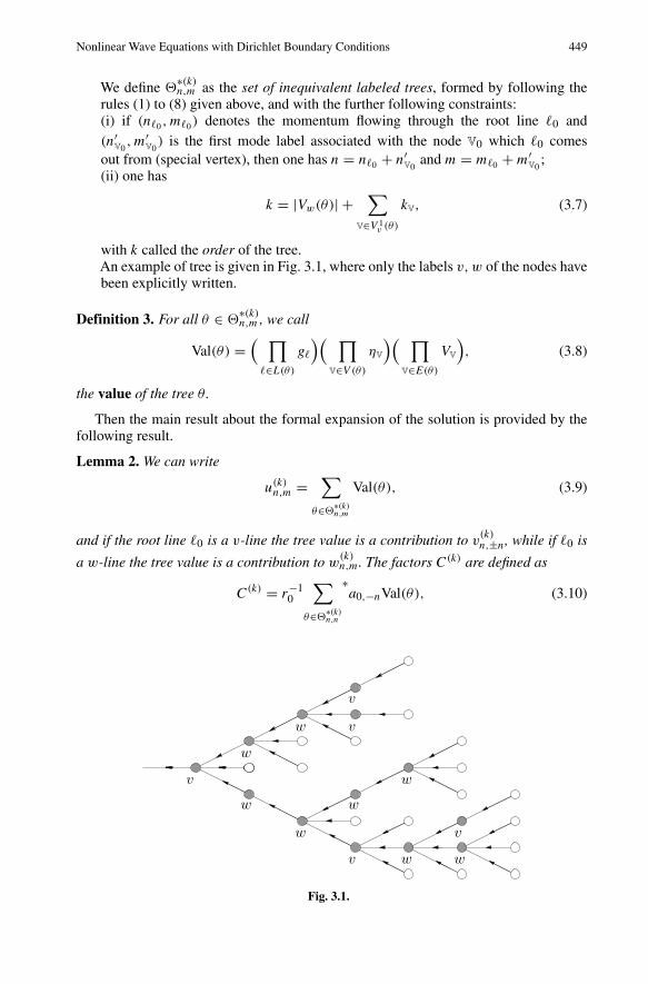
We define �∗(k)n,m as the set of inequivalent labeled trees, formed by following the

rules (1) to (8) given above, and with the further following constraints:(i) if (n�0 , m�0) denotes the momentum flowing through the root line �0 and(n′

V0, m′

V0) is the first mode label associated with the node V0 which �0 comes

out from (special vertex), then one has n = n�0 + n′V0

and m = m�0 + m′V0

;(ii) one has

k = |Vw(θ)| +∑

V∈V 1v (θ)

kV, (3.7)

with k called the order of the tree.An example of tree is given in Fig. 3.1, where only the labels v, w of the nodes havebeen explicitly written.

Definition 3. For all θ ∈ �∗(k)n,m , we call

Val(θ) =( ∏

�∈L(θ)

g�

)( ∏V∈V (θ)

ηV

)( ∏V∈E(θ)

VV

), (3.8)

the value of the tree θ .

Then the main result about the formal expansion of the solution is provided by thefollowing result.

Lemma 2. We can write

u(k)n,m =

∑θ∈�

∗(k)n,m

Val(θ), (3.9)

and if the root line �0 is a v-line the tree value is a contribution to v(k)n,±n, while if �0 is

a w-line the tree value is a contribution to w(k)n,m. The factors C(k) are defined as

C(k) = r−10

∑θ∈�

∗(k)n,n

∗a0,−nVal(θ), (3.10)

Fig. 3.1.

450 G. Gentile, V. Mastropietro, M. Procesi

Fig. 3.2.

Fig. 3.3.

where the ∗ in the sum means the extra constraint sV0 = 3 for the node immediatelypreceding the root (which is the special vertex of the rooted tree).

Proof. The proof is done by induction in k. Imagine to represent graphically a0,n as a(small) white bullet with a line coming out from it, as in Fig. 3.2a, and u

(k)n,m, k ≥ 1, as

a (big) black bullet with a line coming out from it, as in Fig. 3.2b.One should imagine that labels k, n, m are associated with the black bullet represent-

ing u(k)n,m, while a white bullet representing a0,n carries the labels n, m = ±n.

For k = 1 the proof of (3.9) and (3.10) is just a check from the diagrammatic rulesand the recursive definitions (2.27) and (2.29), and it can be performed as follows.

Consider first the case |n| �= |m|, so that u(1)n,m = w

(1)n,m. By taking into account only

the badge labels of the lines, by item (4) there is only one tree whose root line is aw-line, and it has one node V0 (the special vertex of the tree) with sV0 = 3, hence threeend-points V1, V2 and V3. By applying the rules listed above one obtains, for |n| �= |m|,

w(1)n,m = 1

−ω2n2 + ω2m

∑n1+n2+n3=n

m1+m2+m3=m

v(0)n1,m1

v(0)n2,m2

v(0)n3,m3

=∑

θ∈�∗(1)n,m

Val(θ), (3.11)

where the sum is over all trees θ which can be obtained from the tree appearing in Fig. 3.3by summing over all labels which are not explicitly written.

It is easy to realize that (3.11) corresponds to (2.31) for k = 1. Each end-point Vi isgraphically a white bullet with first mode labels (ni, mi) and second mode labels (0, 0),and has associated an end-point factor (−1)1+δni ,mi a0,ni

(see 3.5) in item (7)). The nodeV0 is represented as a (small) gray bullet, with mode labels (0, 0) and (0, 0), and thefactor associated with it is ηV0 = ε (see 3.4) in item (6)). We associate with the line� coming out from the node V0 a momentum (n�, n�), with n� = n, and a propagatorg� = 1/(−ω2n2

� + ω2m�

) (see (3.1) in item (3)).

Now we consider the case |n| = |m|, so that u(1)n,m = ±A

(1)n (see (2.16)). By taking

into account only the badge labels of the lines, there are four trees contributing to A(1)n :

they are represented by the four trees in Fig. 3.4 (the tree b and c are simply obtainedfrom the tree by a different choice of the w-line entering the last node).

Nonlinear Wave Equations with Dirichlet Boundary Conditions 451

Fig. 3.4.

In the trees of Figs. 3.4a, 3.4b and 3.4c the root line comes out from a node V0 (thespecial vertex of the tree) with sV0 = 3, and two of the entering lines come out fromend-points: then the other line has to be a w-line (by item (4)), and (3.7) requires thatthe subtree which has such a line as root line is exactly the tree represented in Fig. 3.2.In the tree of Fig. 4.4d the root line comes out from a node V0 with sV0 = 1, hence theline entering V0 is a v-line coming out from an end-point (again see item (4)).

By defining �∗(1)n,n as the set of all labeled trees which can be obtained by assigning

to the trees in Fig. 3.4 the labels which are not explicitly written, one finds

A(1)n =

∑θ∈�

∗(1)n,n

Val(θ), (3.12)

which corresponds to the sum of two contributions. The first one arises from the treesof Figs. 3.4a, 3.4b and 3.4c, and it is given by

3∑n′∈Z

Ln,n′∑

n′1+n′

2+n′3=n′

m′1+m′

2+m′3=n′

v(0)

n′1,m

′1v

(0)

n′2,m

′2w

(1)

n′3,m

′3, (3.13)

where one has

Ln,n′ = Bm−2m D2

m

∑n1+n2=n−n′

n2=−n′

∗sn1sn2 + Bm

∑n1+n2=n−n′

∗ 1

i2(n2 + n′)2 cdn1cdn2

+ Bm−1m Dm

∑n1+n2=n−n′

∗ 1

i(n2 + n′)sn1cdn2 (3.14)

− Bm−1m Dm

∑n1+n2=n−n′

∗ 1

i(n2 + n′)cdn1sn2 ,

with the ∗ denoting the constraint n2 + n′ �= 0. The first and second mode labels associ-ated with the node V0 are, respectively, (m′

V0, n′

V0) = (n1, n1) and (mV0 , nV0) = (n2, n2),

while the momentum flowing through the root line is given by (n�, m�), with |m�| = |n�|expressed according to the definition (3.6) in item (8): the corresponding propagator is(n�)

δ� for n� �= 0 and 1 for n� = 0, as in (3.1) in item (3).

452 G. Gentile, V. Mastropietro, M. Procesi

Fig. 3.5.

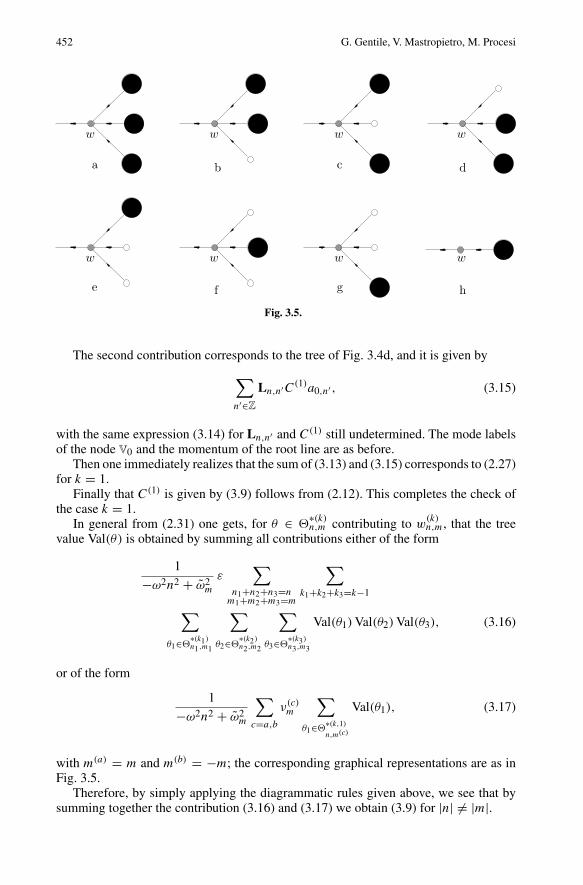
The second contribution corresponds to the tree of Fig. 3.4d, and it is given by

∑n′∈Z

Ln,n′C(1)a0,n′ , (3.15)

with the same expression (3.14) for Ln,n′ and C(1) still undetermined. The mode labelsof the node V0 and the momentum of the root line are as before.

Then one immediately realizes that the sum of (3.13) and (3.15) corresponds to (2.27)for k = 1.

Finally that C(1) is given by (3.9) follows from (2.12). This completes the check ofthe case k = 1.

In general from (2.31) one gets, for θ ∈ �∗(k)n,m contributing to w

(k)n,m, that the tree

value Val(θ) is obtained by summing all contributions either of the form

1

−ω2n2 + ω2m

ε∑

n1+n2+n3=nm1+m2+m3=m

∑k1+k2+k3=k−1

∑θ1∈�

∗(k1)n1,m1

∑θ2∈�

∗(k2)n2,m2

∑θ3∈�

∗(k3)n3,m3

Val(θ1) Val(θ2) Val(θ3), (3.16)

or of the form

1

−ω2n2 + ω2m

∑c=a,b

ν(c)m

∑θ1∈�

∗(k,1)

n,m(c)

Val(θ1), (3.17)

with m(a) = m and m(b) = −m; the corresponding graphical representations are as inFig. 3.5.

Therefore, by simply applying the diagrammatic rules given above, we see that bysumming together the contribution (3.16) and (3.17) we obtain (3.9) for |n| �= |m|.

Nonlinear Wave Equations with Dirichlet Boundary Conditions 453

Fig. 3.6.

A similar discussion applies to A(k)n , and one finds that A

(k)n can be written as a sum

of contribution either of the form∑n′∈Z

Ln,n′∑

n′1+n′

2+n′3=n′

m′1+m′

2+m′3=n′

∑k1+k2+k3=k

∑θ1∈�

∗(k1)n1,m1

∑θ2∈�

∗(k2)n2,m2

∑θ3∈�

∗(k3)n3,m3

Val(θ1) Val(θ2) Val(θ3), (3.18)

or of the form ∑n′∈Z

Ln,n′C(k)a0,n′ , (3.19)

with C(k) still undetermined. Both (3.18) and (3.19) are of the form Val(θ), for θ ∈ �∗(k)n,m .

A graphical representation is in Fig. 3.6.Analogously to the case k = 1 the coefficients C(k) are found to be expressed by

(3.10). Then the lemma is proved. ��Lemma 3. For any rooted tree θ one has |V 3

v (θ)| ≤ 2|V 3w(θ)| + 2|V 1

v (θ)| and |E(θ)| ≤2(|V 3

v (θ)| + |V 3w(θ)|) + 1.

Proof. First of all note that |V 3w(θ)| = 0 requires |V 1

v (θ)| ≥ 1, so that one has |V 3w(θ)|+

|V 1v (θ)| ≥ 1 for all trees θ .We prove by induction on the number N of nodes the bound

∣∣∣V 3v (θ)

∣∣∣ ≤{

2|V 3w(θ)| + 2|V 1

v (θ)| − 1, if the root line is a v-line,2|V 3

w(θ)| + 2|V 1v (θ)| − 2 if the root line is a w-line,

(3.20)

which will immediately imply the first assertion.

For N = 1 the bound is trivially satisfied, as Figs. 3.3 and 3.4 show.Then assume that (3.20) holds for the trees with N ′ nodes, for all N ′ < N , and

consider a tree θ with V (θ) = N .If the special vertex V0 of θ is not in V 3

v (θ) (hence it is in Vw(θ)) the bound (3.20)follows trivially by the inductive hypothesis.

If V0 ∈ V 3v (θ) then we can write

|V 3v (θ)| = 1 +

s∑i=1

|V 3v (θi)|, (3.21)

454 G. Gentile, V. Mastropietro, M. Procesi

where θ1, . . . , θs are the subtrees (not endpoints) whose root line is one of the linesentering V0. One must have s ≥ 1, as s = 0 would correspond to having all the enteringlines of V0 coming out from end-points, hence to having N = 1.

If s ≥ 2 one has from (3.21) and from the inductive hypothesis

|V 3v (θ)| ≤ 1 +

s∑i=1

(2|V 3

w(θi)| + 2|V 1v (θi)| − 1

)≤ 1 + 2|V 3

w(θ)| + 2|V 1v (θ)| − 2,

(3.22)

and the bound (3.20) follows.If s = 1 then the root line of θ1 has to be a w-line by item (4), so that one has

|V 3v (θ)| ≤ 1 +

(2|V 3

w(θ1)| + 2|V 1v (θ)| − 2

)(3.23)

which again yields (3.20).Finally the second assertion follows from the standard (trivial) property of trees

∑V∈V (θ)

(sV − 1) = |E(θ)| − 1, (3.24)

and the observation that in our case one has sV ≤ 3. ��

4. Tree Expansion: The Multiscale Decomposition

We assume the Diophantine conditions (2.33). We introduce a multiscale decompositionof the propagators of the w-lines. Let χ(x) be a C∞ non-increasing function such thatχ(x) = 0 if |x| ≥ 2C0 and χ(x) = 1 if |x| ≤ C0 (C0 is the same constant appearing in(2.33)), and let χh(x) = χ(2hx) − χ(2h+1x) for h ≥ 0, and χ−1(x) = 1 − χ(x); suchfunctions realize a smooth partition of the unity as

1 = χ−1(x) +∞∑

h=0

χh(x) =∞∑

h=−1

χh(x). (4.1)

If χh(x) �= 0 for h ≥ 0 one has 2−h−1C0 ≤ |x| ≤ 2−h+1C0, while if χ−1(x) �= 0 onehas |x| ≥ C0.

We write the propagator of any w-line as the sum of propagators on single scales inthe following way:

g(ωn, m) =∞∑

h=−1

χh(|ωn| − ωm)

−ω2n2 + ω2m

=∞∑

h=−1

g(h)(ωn, m). (4.2)

Note that we can bound |g(h)(ωn, m)| ≤ 2h+1

C0(notice that given n, m there are at

most two non-zero values of g(h)(ωn, m)).This means that we can attach to each w-line � in L(θ) a scale label h� ≥ −1, which

is the scale of the propagator which is associated with �. We can denote with �(k)n,m the set

of trees which differ from the previous ones simply because the lines carry also the scalelabels. The set �

(k)n,m is defined according to the rules (1) to (8) of Sect. 3, by changing

item (3) into the following one.

Nonlinear Wave Equations with Dirichlet Boundary Conditions 455

(3′) With each line � coming out from nodes of w-type we associate a scale label h� ≥ −1.For notational convenience we associate a scale label h = −1 with the lines comingout from the nodes of v-type and with the lines coming out from the end-points. Witheach line � we associate a propagator

g(h�)� ≡ g(h�)(ωn�, m�) =

χh�(|ωn�|−ωm�

)

−ω2n2�+ω2

m�

, if γ� = w,

1(in�)

δ�, if γ� = v, n� �= 0,

1, if γ� = v, n� = 0,

(4.3)

with momentum (n�, m�).

Definition 4. For all θ ∈ �(k)n,m, we define

Val(θ) =( ∏

�∈L(θ)

g(h�)�

)( ∏V∈V (θ)

ηV

)( ∏V∈E(θ)

VV

), (4.4)

the value of the tree θ .

Then (3.9) and (3.10) are replaced, respectively, with

u(k)n,m =

∑θ∈�

(k)n,m

Val(θ), (4.5)

and

C(k) = r−10

∑θ∈�

(k)n,n

∗a0,−nVal(θ), (4.6)

with the new definition for the tree value Val(θ) and with ∗ meaning the same constraintas in (3.10).

Definition 5. A cluster T is a connected set of nodes which are linked by a continuouspath of lines with the same scale label hT or a lower one and which are maximal; weshall say that the cluster has scale hT . We shall denote with V (T ) and E(T ) the set ofnodes and the set of end-points, respectively, which are contained inside the cluster T ,and with L(T ) the set of lines connecting them. As for trees we call Vv(T ) and Vw(T )

the sets of nodes V ∈ V (T ) which are of v-type and of w-type respectively. Analogouslyone defines the sets V s

v (T ) and V sw(T ).

We define the order kT of a cluster T as the order of a tree (see item (ii) beforeDefinition 3), with the sums restricted to the nodes internal to the cluster.

An inclusion relation is established between clusters, in such a way that the inner-most clusters are the clusters with lowest scale, and so on. Each cluster T can have anarbitrary number of lines entering it (incoming lines), but only one or zero line comingfrom it (outcoming line); we shall denote the latter (when it exists) with �1

T . We shall callexternal lines of the cluster T the lines which either enter or come out from T , and weshall denote by h

(e)T the minimum among the scales of the external lines of T . Define also

K(θ) =∑

V∈V (θ)

(|n′V| + |nV|)+

∑V∈E(θ)

|n′V|,

K(T ) =∑

V∈V (T )

(|n′V| + |nV|)+

∑V∈E(θ)

|n′V|, (4.7)

456 G. Gentile, V. Mastropietro, M. Procesi

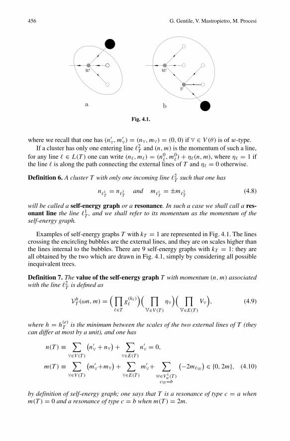
Fig. 4.1.

where we recall that one has (n′V, m′

V) = (nV, mV) = (0, 0) if V ∈ V (θ) is of w-type.

If a cluster has only one entering line �2T and (n, m) is the momentum of such a line,

for any line � ∈ L(T ) one can write (n�, m�) = (n0�, m

0�) + η�(n, m), where η� = 1 if

the line � is along the path connecting the external lines of T and η� = 0 otherwise.

Definition 6. A cluster T with only one incoming line �2T such that one has

n�1T

= n�2T

and m�1T

= ±m�2T

(4.8)

will be called a self-energy graph or a resonance. In such a case we shall call a res-onant line the line �1

T , and we shall refer to its momentum as the momentum of theself-energy graph.

Examples of self-energy graphs T with kT = 1 are represented in Fig. 4.1. The linescrossing the encircling bubbles are the external lines, and they are on scales higher thanthe lines internal to the bubbles. There are 9 self-energy graphs with kT = 1: they areall obtained by the two which are drawn in Fig. 4.1, simply by considering all possibleinequivalent trees.

Definition 7. The value of the self-energy graph T with momentum (n, m) associatedwith the line �2

T is defined as

VhT (ωn, m) =

(∏�∈T

g(h�)�

)( ∏V∈V (T )

ηV

)( ∏V∈E(T )

VV

), (4.9)

where h = h(e)T is the minimum between the scales of the two external lines of T (they

can differ at most by a unit), and one has

n(T ) ≡∑

V∈V (T )

(n′

V+ nV

)+∑

V∈E(T )

n′V

= 0,

m(T ) ≡∑

V∈V (T )

(m′

V+mV

)+∑

V∈E(T )

m′V+

∑W∈V 1

w(T )cW=b

(−2m�W

) ∈ {0, 2m}, (4.10)

by definition of self-energy graph; one says that T is a resonance of type c = a whenm(T ) = 0 and a resonance of type c = b when m(T ) = 2m.

Nonlinear Wave Equations with Dirichlet Boundary Conditions 457

Definition 8. Given a tree θ , we shall denote by Nh(θ) the number of lines with scaleh, and by Ch(θ) the number of clusters with scale h.

Then the product of propagators appearing in (4.4) can be bounded as

∣∣∣ ∏�∈L(θ)

g(h�)�

∣∣∣ ≤ (∞∏

h=0

2hNh(θ))( ∏

�∈L(θ)γ�=w

χh�(|ωn�| − ωm�

)

|ωn�| + ωm�

)( ∏�∈L(θ)

γ�=v, n� �=0

1

|ωn�|),

(4.11)

and this will be used later.

Lemma 4. Assume 0 < C0 < 1/2 and that there is a constant C1 such that one has|ωm − |m|| ≤ C1ε/|m|. If ε is small enough for any tree θ ∈ �

(k)n,m and for any line � on

a scale h� ≥ 0 one has min{m�, n�} ≥ 1/2ε.

Proof. If a line � with momentum (n, m) is on scale h ≥ 0 then one has

1

2> C0 ≥ ||ωn| − ωm| ≥

∣∣∣(√1 − ε − 1)

|n| + (|n| − |m|) − C1ε/|m|∣∣∣

≥∣∣∣∣∣∣∣∣ ε |n|1 + √

1 − ε− (|n| − |m|)

∣∣∣∣− C1ε/|m|∣∣∣∣ , (4.12)

with |n| �= |m|, hence |n−m| ≥ 1, so that |n| ≥ 1/2ε. Moreover one has ||ωn|− ωm| ≤1/2 and ωm − |m| = O(ε), and one obtains also |m| > 1/2ε. ��Lemma 5. Define h0 such that 2h0 ≤ 16C0/ε < 2h0+1, and assume that there is aconstant C1 such that one has |ωm − |m|| ≤ C1ε/|m|. If ε is small enough for any treeθ ∈ �

(k)n,m and for all h ≥ h0 one has

Nh(θ) ≤ 4K(θ)2(2−h)/τ − Ch(θ) + Sh(θ) + Mνh(θ), (4.13)

where K(θ) is defined in (4.7), while Sh(θ) is the number of self-energy graphs T in θ

with h(e)T = h and Mν

h(θ) is the number of ν-vertices in θ such that the maximum scaleof the two external lines is h.

Proof. We prove inductively the bound

N∗h (θ) ≤ max{0, 2K(θ)2(2−h)/τ − 1}, (4.14)

where N∗h (θ) is the number of non-resonant lines in L(θ) on scale h′ ≥ h.

First of all note that for a tree θ to have a line on scale h the condition K(θ) > 2(h−1)/τ

is necessary, by the first Diophantine conditions in (2.33). This means that one can haveN∗

h (θ) ≥ 1 only if K = K(θ) is such that K > k0 ≡ 2(h−1)/τ : therefore for valuesK ≤ k0 the bound (4.14) is satisfied.

If K = K(θ) > k0, we assume that the bound holds for all trees θ ′ with K(θ ′) < K .Define Eh = 2−1(2(2−h)/τ )−1: so we have to prove that N∗

h (θ) ≤ max{0, K(θ)E−1h −1}.

Call � the root line of θ and �1, . . . , �m the m ≥ 0 lines on scale ≥ h which are theclosest to � (i.e. such that no other line along the paths connecting the lines �1, . . . , �m

to the root line is on scale ≥ h).

458 G. Gentile, V. Mastropietro, M. Procesi

If the root line � of θ is either on scale < h or on scale ≥ h and resonant, then

N∗h (θ) =

m∑i=1

N∗h (θi), (4.15)

where θi is the subtree with �i as root line, hence the bound follows by the inductivehypothesis.

If the root line � has scale ≥ h and is non-resonant, then �1, . . . , �m are the enteringline of a cluster T .

By denoting again with θi the subtree having �i as root line, one has

N∗h (θ) = 1 +

m∑i=1

N∗h (θi), (4.16)

so that the bound becomes trivial if either m = 0 or m ≥ 2.If m = 1 then one has a cluster T with two external lines � and �1, which are both

with scales ≥ h; then∣∣|ωn�| − ωm�

∣∣ ≤ 2−h+1C0,

∣∣∣|ωn�1 | − ωm�1

∣∣∣ ≤ 2−h+1C0, (4.17)

and recall that T is not a self-energy graph.Note that the validity of both inequalities in (4.17) for h ≥ h0 imply that one has

|n� − n�1 | �= |m� ± m�1 |, as we are going to show.By Lemma 4 we know that one has min{m�, n�} ≥ 1/2ε. Then from (4.17) we have,

for some η�, η�1 ∈ {±1},2−h+2C0 ≥ ∣∣ω(n� − n�1) + η�ωm�

+ η�1 ωm�1

∣∣, (4.18)

so that if one had |n� − n�1 | = |m� ± m�1 | we would obtain for ε small enough

2−h+2C0 ≥ ε

1 + √1 − ε

∣∣n� − n�1

∣∣− C1ε

|m�| − C1ε

|m�1 |≥ ε

2− 4C1ε

2 >ε

4, (4.19)

which is contradictory with h ≤ h0; hence one has |n� − n�1 | �= |m� ± m�1 |.Then, by (4.17) and for |n�−n�1 | �= |m�±m�1 |, one has, for suitable η�, η�1 ∈ {+, −},

2−h+2C0 ≥ ∣∣ω(n� − n�1) + η�ωm�+ η�1 ωm�1

∣∣ ≥ C0|n� − n�1 |−τ , (4.20)

where the second Diophantine conditions in (2.33) have been used. Hence K(θ) −K(θ1) > Eh, which, inserted into (4.16) with m = 1, gives, by using the inductivehypothesis,

N∗h (θ) = 1 + N∗

h (θ1) ≤ 1 + K(θ1)E−1h − 1

≤ 1 +(K(θ) − Eh

)E−1

h − 1 ≤ K(θ)E−1h − 1, (4.21)

hence the bound is proved also if the root line is on scale ≥ h.In the same way one proves that, if we denote with Ch(θ) the number of clusters on

scale h, one has

Ch(θ) ≤ max{0, 2K(θ)2(2−h)/τ − 1}; (4.22)

see [23] for details. ��

Nonlinear Wave Equations with Dirichlet Boundary Conditions 459

Note that the argument above is very close to [23]: this is due to the fact that theexternal lines of any self-energy graph T are both w-lines, so that the only effect of thepresence of the v-lines and of the nodes of v-type is in the contribution to K(T ).

The following lemma deals with the lines on scale h < h0.

Lemma 6. Let h0 be defined as in Lemma 2 and C0 < 1/2, and assume that there is aconstant C1 such that one has |ωm − |m|| ≤ C1ε. If ε is small enough for h < h0 onehas |g(h)

� | ≤ 32.

Proof. Either if h �= h� or h = h� = −1 the bound is trivial. If h = h� ≥ 0 one has

g(h)� = χh(|ωn�| − ωm�

)

−|ωn�| + ωm

1

|ωn�| + ωm

, (4.23)

where |ωn�| + ωm ≥ 1/2ε by Lemma 4. Then one has

1

|ωn�| + ωm

≤ 2ε, (4.24)

which, inserted in (4.23), gives |g(h)� | ≤ 2h+2ε/C0 ≤ 32, so that the lemma is proved.

��

5. The Renormalized Expansion

It is an immediate consequence of Lemma 5 and Lemma 6 that all the trees θ with noself-energy graphs or ν-vertices admit a bound O(Ckεk), where C is a constant. Howeverthe generic tree θ with Sh(θ) �= 0 admits a much worse bound, namely O(Ckεkk!α), forsome constant α, and the presence of factorials prevent us to prove the convergence ofthe series; in KAM theory this is called accumulation of small divisors. It is convenientthen to consider another expansion for un,m, which is essentially a resummation of theone introduced in Sects. 3 and 4.

We define the set �(k)Rn,m of renormalized trees, which are defined as �

(k)n,m except that

the following rules are added.

(9) To each self-energy graph (with |m| ≥ 1) the R = � − L operation is applied,where L acts on the self-energy graphs in the following way, for h ≥ 0 and |m| ≥ 1,

LVhT (ωn, m) = Vh

T (sgn(n) ωm, m), (5.1)

R is called a regularization operator; its action simply means that each self-energygraph Vh

T (ωn, m) must be replaced by RVhT (ωn, m).

(10) With the nodes V of w-type with sV = 1 (which we still call ν-vertices) and withh ≥ 0 the minimal scale among the lines entering or exiting V, we associate a factor2−hν

(c)h,m, c = a, b, where (n, m) and (n, ±m), with |m| ≥ 1, are the momenta of

the lines and a corresponds to the sign + and b to the sign − in ±m.(11) The set {h�} of the scales associated with the lines � ∈ L(θ) must satisfy the follow-

ing constraint (which we call compatibility): fixed (n�, m�) for any � ∈ L(θ) andreplaced R with � at each self-energy graph, one must have χh�

(|ωn�|− ωm�) �= 0.

(12) The factors C(kV) in (3.3) are replaced with �, to be considered a parameter.

460 G. Gentile, V. Mastropietro, M. Procesi

The set �(k)Rn,m is defined as �

(k)n,m with the new rules and with the constraint that the

order k is given by k = |Vw(θ)| + |V 1v (θ)|.

We consider the following expansion

un,m =∞∑

k=1

µk∑

θ∈�(k)Rn,m

Val(θ), (5.2)

where, for |m| ≥ 1 and h ≥ 0, ν(c)h,m is given by

2−hµν(c)h,m = µν(c)

m + 1

2

∑σ=±

∑T ∈T (c)

<h

µkT VhT (σ ωm, m), (5.3)

with c = a, b, and T (c)<h denoting the set of self-energy graphs T of type c (see item (6)

in Sect. 3) with hT < h, and � is determined by the self-consistence equation

� = r−10

∞∑k=1

µk−1∑

θ∈�(k)Rn,n

∗a0,−nVal(θ), (5.4)

with ∗ denoting the same constraint as in (3.10).We shall set also ν

(c)m = ν

(c)−1,m. Note that Vh

T (σ ωm, m) is independent of σ .Calling L0(θ), V0(θ), E0(θ) the set of lines, node and end-points not contained in

any self-energy graph, and S0(θ) the maximal self-energy graphs, i.e. the self-energygraphs which are not contained in any self-energy graphs, we can write Val(θ) in (5.2)as

Val(θ) =( ∏

�∈L0(θ)

g(h�)�

)( ∏V∈V0(θ)

ηV

)( ∏V∈E0(θ)

VV

)( ∏T ∈S0(θ)

RVheT

T (ωn�T, m�T

)),

(5.5)

and by definition

RVheT

T (ωn�T, m�T

) = VheT

T (ωn�T, m�T

) − VheT

T (sgn(n�T) ωm�T

, m�T), (5.6)

and VheT

T (ωn�T, m�T

) is given by

VheT

T (ωn�T, m�T

) =( ∏

�∈L0(T )

g(h�)

�

)( ∏V∈V0(T )

ηV

)( ∏V∈E0(T )

VV

)( ∏T ′∈S0(T )

RVheT ′

T ′ (ωn�T ′ , m�T ′ )).

(5.7)

First (Lemma 7) we will show that the expansion (5.2) is well defined, for νh,m, � =O(ε); then (Lemmas 8 and 9) we show that under the same conditions also the r.h.s. of(5.3) is well defined; moreover (Lemma 10) we prove by using (5.3) that it is indeedpossible to choose ν

(c)m such that νh,m = O(ε) for any h; then (Lemmas 11 and 12) we

show that (5.2) admit a solution � = O(ε); finally (Lemma 13) we show that indeed(5.2) solves the last of (1.14) and (2.2); this completes the proof of Proposition 1. In thenext section we will solve the implicit function problem of (2.1), thus completing theproof of Theorem 1.

We start from the following lemma stating that, if the ν(c)h,m and � functions are

bounded, then the expansion (5.2) is well defined.

Nonlinear Wave Equations with Dirichlet Boundary Conditions 461

Lemma 7. Assume that there exist a constant C such that one has |�| ≤ Cε and |ν(c)h,m| ≤

Cε, with c = a, b, for all |m| ≥ 1 and all h ≥ 0. Then for all µ0 > 0 there exists ε0 > 0such that for all |µ| ≤ µ0 and for all 0 < ε < ε0 and for all (n, m) ∈ Z

2 one has∣∣un,m

∣∣ ≤ D0εµ e−κ(|n|+|m|)/4, (5.8)

where D0 is a positive constant. Moreover un,m is analytic in µ and in the parameters

ν(c)

m′,h′ , with c = a, b and |m′| ≥ 1.

Proof. In order to take into account the R operation we write (5.6) as

RVheT

T (ωn�T, m�T

) =(ωn�T

− ωm�T

) ∫ 1

0dt∂Vhe

T

T (ωn�T+ t (ωn�T

− ωm�T), m�T

),

(5.9)

where ∂ denotes the derivative with respect to the argument ωn�T+ t (ωn�T

− ωm�T).

By (5.7) we see that the derivatives can be applied either on the propagators in L0(T ),

or on the RVhe

T ′T ′ . In the first case there is an extra factor 2−h

(e)T +hT with respect to the

bound (4.11): 2−h(e)T is obtained from ωn�T

− ωm�Twhile ∂g(hT ) is bounded proportion-

ally to 22hT ; in the second case note that ∂tRVhe

T ′T ′ = ∂tV

heT ′

T ′ as LVh

(e)

T ′T ′ is independent of

t ; if the derivative acts on the propagator of a line � ∈ L(T ), we get a gain factor

2−h(e)T +hT ′ ≤ 2−h

(e)T +hT 2−h

(e)

T ′ +hT ′ , (5.10)

as h(e)

T ′ ≤ hT . We can iterate this procedure until all the R operations are applied onpropagators; at the end (i) the propagators are derived at most one time; (ii) the number

of terms so generated is ≤ k; (iii) with each self-energy graph T a factor 2−h(e)T +hT is

associated.Assuming that |ν(c)

h,m| ≤ Cε and |�| ≤ Cε, for any θ one obtains, for a suitable

constant D,

|Val(θ)| ≤ ε|Vw(θ)|+|V (1)v (θ)|D|V (θ)|

( ∞∏h=h0

exp[h log 2

(4K(θ)2−(h−2)/τ − Ch(θ) + Sh(θ) + Mν

h(θ))])

( ∏T ∈S(θ)

h(e)T

≥h0

2−h(e)T +hT

)( ∞∏h=h0

2−hMνh(θ))

(5.11)

( ∏V∈V (θ)∪E(θ)

e−κ(|nV|+|n′V|))( ∏

V∈V (θ)∪E(θ)

e−κ(|mV|+|m′V|)),

where the second line is a bound for∏

h≥h02hNh(θ) and we have used that by item (12)

Nh(θ) can be bounded through Lemma 5, and Lemma 4 has been used for the lineson scales h < h0; moreover

∏∞h=h0

2−hMhν (θ) takes into account the factors 2−h arising

from the running coupling constants ν(c)h,m and the action of R produces, as discussed

above, the factor∏

T ∈S(θ) 2−h(e)T +hT . Then one has

462 G. Gentile, V. Mastropietro, M. Procesi

( ∞∏h=h0

2hSh(θ))( ∏

T ∈S(θ)

2−h(e)T

)= 1,

( ∞∏h=h0

2−hCh(θ))( ∏

T ∈S(θ)

2hT

)≤ 1. (5.12)

We have to sum the values of all trees, so we have to worry about the sum of the labels.Recall that a labeled tree is obtained from an unlabeled tree by assigning all the labels tothe points and the lines: so the sum over all possible labeled trees can be written as sumover all unlabeled trees and of labels. For a fixed unlabeled tree θ with a given number ofnodes, say N , we can assign first the mode labels {(n′

V, m′

V), (nV, mV)}v∈V (θ)∪E(θ), and

we sum over all the other labels, which gives 4|Vv(θ)| (for the labels jV) times 2|L(θ)| (forthe scale labels): then all the other labels are uniquely fixed. Then we can perform thesum over the mode labels by using the exponential decay arising from the node factors(3.3) and end-point factors (3.4). Finally we have to sum over the unlabeled trees, and thisgives a factor 4N [26]. By Lemma 3, one has |V (θ)| = |Vw(θ)|+|V (1)

v (θ)|+|V (3)v (θ)| ≤

3(|V (3)w (θ)| + |V (1)

v (θ)|), hence N ≤ 3k, so that∑

θ∈�(k)Rn,m

|Val(θ)| ≤ Dkεk , for some

positive constant D.Therefore, for fixed (n, m) one has

∞∑k=1

∑θ∈�

(k)n,m

µk |Val(θ)| ≤ D0µε e−κ(|n|+|m|)/4, (5.13)

for some positive constant D0, so that (5.8) is proved. ��From (5.3) we know that the quantities ν

(c)h,m, for h ≥ 0 and |m| ≥ 1, verify the

recursive relations

µν(c)h+1,m = 2µν

(c)h,m + β

(c)h,m(ω, ε, {ν(c′)

h′,m′ }), (5.14)

where, by defining T (c)h as the set of self-energy graphs in T (c)

<h+1 which are on scale h,the beta function

β(c)h,m ≡ β

(c)h,m(ω, ε, {ν(c′)

h′,m′ }) = 2h+1 1

2

∑σ=±

∑T ∈T (c)

h

µkT Vh+1T (σ ωm, m), (5.15)

depends only on the scales h′ ≤ h.In order to obtain a bound on the beta function, hence on the running coupling con-

stants, we need to bound Vh+1T (±ωm, m) for T ∈ T (c)

h . We define �(k)Rn,m as the set �(k)R

n,m

introduced before, but by changing item (7) into the following one:

(7′) We divide the set E(θ) of end-points into two sets E(θ) and E0(θ). With each end-point V ∈ E(θ) we associate a first mode label (n′

V, m′

V), with |m′

V| = |n′

V|, a second

mode label (0, 0) and an end-point factor VV = (−1)1+δn′

V,m′

V a0,n′V

, while E0(θ) iseither the empty set or a single end-point V0, and, in the latter case, with the end-pointV ∈ E0(θ) we associate a first mode label (ωmV

, nV), where ωmV= ωmV

/ω, a secondmode label (0, 0) and an end-point factor VV = 1.

Then we have the following generalization of Lemma 4.

Nonlinear Wave Equations with Dirichlet Boundary Conditions 463

Lemma 8. If ε is small enough for any tree θ ∈ �(k)Rn,m one has

Nh(θ) ≤ 4K(θ)2(2−h)/τ − Ch(θ) + Sh(θ) + Mνh(θ), (5.16)

where the notations are as in Lemma 4.

Proof. Lemma 4 holds for E0(θ) = 0; we mimic the proof of Lemma 4 proving that

N∗h (θ) ≤ max{0, 2K(θ)2(2−h)/τ }, (5.17)

for all trees θ with E0(θ) �= ∅, again by induction on K(θ).For any line � ∈ L(θ) set η� = 1 if the line is along the path connecting V0 to the

root and η� = 0 otherwise, and write

n� = n0� + η�ωm, m� = m0

� + η�m, (5.18)

which implicitly defines n0� and m0

� .Define k0 = 2(h−1)/τ . One has N∗

h (θ) = 0 for K(θ) < k0, because if a line � ∈ L(θ)

is indeed on scale h then |ωn� − ωm�| < C021−h, so that (5.18) and the Diophantine

conditions imply

K(θ) ≥∣∣∣n0

�

∣∣∣ > 2(h−1)/τ ≡ k0. (5.19)

Then, for K ≥ k0, we assume that the bound (5.17) holds for all K(θ) = K ′ < K , andwe show that it follows also for K(θ) = K .

If the root line � of θ is either on scale < h or on scale ≥ h and resonant, the bound(5.17) follows immediately from the bound (4.13) and from the inductive hypothesis.

The same occurs if the root line is on scale ≥ h and non-resonant, and, by calling�1, . . . , �m the lines on scale ≥ h which are the closest to �, one has m ≥ 2: in fact insuch a case at least m − 1 among the subtrees θ1, . . . , θm having �1, . . . , �m, respec-tively, as root lines have E0(θi) = ∅, so that we can write, by (4.13) and by the inductivehypothesis,

N∗h (θ) = 1 +

m∑i=1

N∗h (θi) ≤ 1 + E−1

h

m∑i=1

K(θi) − (m − 1) ≤ EhK(θ), (5.20)

so that (5.17) follows.If m = 0 then N∗

h (θ) = 1 and K(θ)2(2−h)/τ ≥ 1 because one must have K(θ) ≥ k0.So the only non-trivial case is when one has m = 1. If this happens �1 is, by con-

struction, the root line of a tree θ1 such that K(θ) = K(T ) + K(θ1), where T is thecluster which has � and �1 as external lines and K(T ), defined in (4.7), satisfies thebound K(T ) ≥ |n�1 − n�|.

Moreover, if E0(θ1) �= ∅, one has∣∣∣|ωn0

� + ωm| − ωm�

∣∣∣ ≤ 2−h+1C0,∣∣∣|ωn0�1

+ ωm| − ωm�1

∣∣∣ ≤ 2−h+1C0, (5.21)

so that, for suitable η�, η�1 ∈ {−, +}, we obtain

464 G. Gentile, V. Mastropietro, M. Procesi

2−h+2C0 ≥ ∣∣ω(n0� − n0

�1) + η�ωm�

+ η�1 ωm�1

∣∣ ≥ C0|n0� − n0

�1|−τ ≡ C0|n� − n�1 |−τ ,

(5.22)

by the second Diophantine conditions in (2.33), as the quantities ωm appearing in (5.21)cancel out. Therefore one obtains by the inductive hypothesis

N∗h (θ) ≤ 1 + K(θ1)E

−1h ≤ 1 + K(θ)E−1

h − K(T )E−1h ≤ K(θ)E−1

h , (5.23)

hence the first bound in (5.17) is proved.If E0(θ1) = ∅, one has

N∗h (θ) ≤ 1 + K(θ1)E

−1h − 1 ≤ 1 + K(θ)E−1

h − 1 ≤ K(θ)E−1h , (5.24)

and (5.17) follows also in such a case. ��The following bound for Vh+1

T (±ωm, m), h ≥ h0, can then be obtained.

Lemma 9. Assume that there exists a constant C such that one has |�| ≤ Cε and|ν(c)

h,m| ≤ Cε, with c = a, b, for all |m| ≥ 1 and all h ≥ 0. Then if ε is small enough for

all h ≥ 0 and for all T ∈ T (c)h one has

|Vh+1T (±ωm, m)| ≤ B |V (T )|e−κ2(h−1)/τ /4e−κK(T )/4ε|V (1)

v (T )|+|Vw(T )|, (5.25)

where B is a constant and K(T ) is defined in (4.7).

Proof. By using Lemma 7 we obtain for all T ∈ T (c)h and assuming h ≥ h0 we get the

bound ∣∣∣Vh+1T (±ωm, m)

∣∣∣ ≤ B|V (T )|

ε|V (1)v (T )|+|Vw(T )|

h∏h′=h0

exp[4K(T ) log 2h′2(2−h′)/τ − Ch′(T ) + Sh′(T ) + Mν

h′(T )]

( ∏T ′⊂T

h(ε)T

≥h0

2−h(e)T +hT

)( h∏h′=h0

2−h′Mνh′ (T )

)e−κ|K(T )|/2, (5.26)

where B is a suitable constant. If h < h0 the bound trivializes as the r.h.s. reduces simply

to C|V (T )||ε||V (1)v (T )|+|Vw(T )|e− κ

2 |K(T )|. The main difference with respect to Lemma 6 isthat, given a self-energy graph T ∈ T (c)

h , there is at least a line � ∈ L(T ) on scale h� = h

and with propagator

1

−ω2(n0� + η�ωm)2 + ω2

m0�+η�m

, (5.27)

where η� = 1 if the line � belongs to the path of lines connecting the entering line (car-rying a momentum (n, m)) of T with the line coming out of T , and η� = 0 otherwise.Then one has by the Mel’nikov conditions

Nonlinear Wave Equations with Dirichlet Boundary Conditions 465

C0|n0�|−τ ≤

∣∣∣ωn0� + η�ωm ± ωm0

�+η�m

∣∣∣ ≤ C02−h+1, (5.28)

so that |n0�| ≥ 2(h−1)/τ . On the other hand one has |n0

�| ≤ K(T ), hence K(T ) ≥ 2(h−1)/τ ;so we get the bound (5.25). ��

It is an immediate consequence of the above lemma that for all µ0 > 0 there existsε0 > 0 such that for all |µ| ≤ µ0 and 0 < ε < ε0 one has |β(c)

h,m| ≤ B1ε|µ|, with B1 asuitable constant.

We have then proved convergence assuming that the parameters νh,m and � arebounded; we have to show that this is actually the case, if the ν

(c)m in (2.34) are chosen

in a proper way.We start proving that it is possible to choose ν(c) = {ν(c)

m }|m|≥1 such that, for a suitable

positive constant C, one has |ν(c)h,m| ≤ Cε for all h ≥ 0 and for all |m| ≥ 1.

For any sequence a ≡ {am}|m|≥1 we introduce the norm

‖a‖∞ = sup|m|≥1

|am|. (5.29)

Then we have the following result.

Lemma 10. Assume that there exists a constant C such that |�| ≤ Cε. Then for allµ0 > 0 there exists ε0 > such that for all |µ| ≤ µ0 and for all 0 < ε < ε0 there

is a family of intervals I(h)c,m, h ≥ 0, |m| ≥ 1, c = a, b, such that I

(h+1)c,m ⊂ I

(h)c,m,

|I hc,m| ≤ 2ε(

√2)−(h+1) and, if ν

(c)m ∈ I

(h)c,m, then

‖ν(c)h ‖∞ ≤ Dε, h ≥ h ≥ 0, (5.30)

for some positive constant D. Finally one has ν(c)h,−m = ν

(c)h,m, c = a, b, for all h ≥ h ≥ 0

and for all |m| ≥ 1. Therefore one has ‖νh‖∞ ≤ Cε for all h ≥ 0, for some positiveconstant D; in particular |νm| ≤ Dε for all m ≥ 1.

Proof. The proof is done by induction on h. Let us define J(h)c,m = [−ε, ε] and call

J (h) =×|m|≥1,c=a,bJ(h)c,m and I (h) = ×|m|≥1,c=a,bI

(h)c,m.

We suppose that there exists I (h) such that, if ν spans I (h) then νh spans J (h) and

|ν(c)h,m| ≤ Dε for h ≥ h ≥ 0; we want to show that the same holds for h + 1. Let us call

J (h+1) the interval spanned by {ν(c)

h+1,m}|m|≥1,c=a,b when {ν(c)

m }|m|≥1,c=a,b span I (h). For

any {ν(c)m }|m|≥1,c=a,b ∈ I (h) one has {νh+1,m}|m|≥1,c=a,b ∈ [−2ε − Dε2, 2ε + Dε2],

where the bound (5.25) has been used. This means that J (h+1) is strictly contained inJ (h+1). On the other hand it is obvious that there is a one-to-one correspondence between{ν(c)

m }|m|>1,c=a,b and the sequence {ν(c)h,m}|m|≥1,c=a,b, h + 1 ≥ h ≥ 0. Hence there is a

set I (h+1) ⊂ I (h) such that, if {ν(c)m }|m|≥1,c=a,b spans I (h+1), then {ν(c)

h+1,m}|m|≥1,c=a,b

spans the interval J (h) and, for ε small enough, |νh|∞ ≤ Cε for h + 1 ≥ h ≥ 0.

466 G. Gentile, V. Mastropietro, M. Procesi

The previous computations also show that the inductive hypothesis is verified also forh = 0 so that we have proved that there exists a decreasing sets of intervals I (h) such thatif {ν(c)

m }|m|>1,c=a,b ∈ I (h) then the sequence {ν(c)h,m}|m|≥1,c=a,b is well defined for h ≤ h

and it verifies |ν(c)h,m| ≤ C|ε|. In order to prove the bound on the size of I

(h)c,m let us denote

by {ν(c)h,m}|m|≥1,c=a,b and {ν′(c)

h,m}|m|≥1,c=a,b, 0 ≤ h ≤ h, the sequences corresponding to

{ν(c)m }|m|≥1,c=a,b and {ν′(c)

m }|m|≥1,c=a,b in I (h). We have

µν(c)h+1,m − µν

′(c)h+1,m = 2

(µν

(c)h,m − µν

′(c)h,m

)+ β

(c)h,m − β

′(c)h,m, (5.31)

where β(c)h,m and β

′(c)h,m are shorthands for the beta functions. Then, as |νk − ν′

k|∞ ≤|νh − ν′

h|∞ for all k ≤ h, we have

|νh − ν′h|∞ ≤ 1

2|νh+1 − ν′

h+1|∞ + Dε2|νh − ν′h|∞. (5.32)

Hence if ε is small enough then one has

‖ν − ν′‖∞ ≤ (√

2)−(h+1)‖νh − ν′h‖∞. (5.33)

Since, by definition, if ν spans I (h), then νh spans the interval J (h), of size 2|ε|, the

size of I (h) is bounded by 2|ε|(√2)(−h−1).Finally note that one can choose ν

(c)m = ν

(c)−m and then ν

(c)h,m = ν

(c)h,−m for any |m| ≥ 1

and any h ≥ h ≥ 0; this follows from the fact that the function β(c)k,m in (5.15) is even

under the exchange m → −m; it depends on m through ωm (which is an even function ofm), through the end-points v ∈ E(θ) (which are odd under the exchange m → −m; buttheir number must be even) and finally through ν

(q−1)k,m which are assumed inductively

to be even. ��It will be useful to explicitly construct the ν

(c)h,m by a contraction method. By iterating

(5.14) we find, for |m| ≥ 1,

µν(c)h,m = 2h+1

(µν(c)

m +h−1∑

k=−1

2−k−2β(c)k,m(ω, ε, {ν(c′)

k′,m′ }))

, (5.34)

where β(c)k,m(ω, ε, {ν(c′)

k′,m′ }) depends on νk′,m′ with k′ ≤ k − 1. If we put h = h in (5.34)we get

µν(c)m = −

h−1∑k=−1

2−k−2β(c)k,m(ω, ε, {ν(c′)

k′,m′ }) + 2−h−1µν(c)

h,m(5.35)

and, combining (5.34) with (5.35), we find, for h > h ≥ 0,

µν(c)h,m = −2h+1

h−1∑

k=h

2−k−2β(c)k,m(ω, ε, {ν(c′)

k′,m′ })+ 2h−hµν

(c)

h,m. (5.36)

Nonlinear Wave Equations with Dirichlet Boundary Conditions 467

The sequences {ν(c)h,m}|m|>1, h > h ≥ h0, parameterized by {ν(c)

h,m}|m|≥2 such that

‖ν(c)

h‖∞ ≤ Cε, can be obtained as the limit as q → ∞ of the sequences {ν(c)(q)

h,m },q ≥ 0, defined recursively as

µν(c)(0)h,m = 0,

µν(c)(q)h,m = −2h+1

h−1∑

k=h

2−k−2β(c)k,m(ω, ε, {ν(c′)(q−1)

k′,m′ })+ 2h−hµν

(c)

h,m. (5.37)

In fact, it is easy to show inductively that, if ε is small enough, ‖ν(q)h ‖∞ ≤ Cε, so

that (5.25) is meaningful, and

max0≤h≤h

‖ν(q)h − ν

(q−1)h ‖∞ ≤ (Cε)q . (5.38)

For q = 1 this is true as ν(c)(0)h = 0; for q > 1 it follows by the fact that

β(c)k (ω, ε, {ν(c′)(q−1)

k′,m′ })−β(c)k (ω, ε, {ν(c′)(q−2)

k′,m′ }) can be written as a sum of terms in which

there are at least one ν-vertex, with a difference ν(c′)(q−1)

h′ − ν(c′)(q−2)

h′ , with h′ ≥ k, in

place of the corresponding ν(c′)h′ , and one node carrying an ε. Then ν

(q)h converges as

q → ∞, for h < h ≤ 1, to a limit νh, satisfying the bound ‖νh‖∞ ≤ Cε. Since thesolution is unique, it must coincide with one in Lemma 10.

We have then constructed a sequence of ν(c)h,m solving (5.36) for any h > 1 and any

ν(c)

h,m; we shall call ν

(c)h,m(�) the solution of (5.36) with h = ∞ and ν

(c)∞,m = 0, to stress

the dependence on �.We will prove the following lemma.

Lemma 11. Under the the same conditions of Lemma 10 it holds that for any h ≥ 0,

‖νh(�1) − νh(�

2)‖∞ ≤ Dε|�1 − �2|, (5.39)

for a suitable constant D.

Proof. Calling ν(q)h (�) the l.h.s. of (5.25) with h = ∞ and ν∞,m = 0, we can show by

induction on q that

‖ν(q)h (�1) − ν

(q)h (�2)‖∞ ≤ Dε|�1 − �2|. (5.40)

We find convenient to write explicitly the dependence of the function β(c)h,m from the

parameter �, so that we rewrite β(c)k,m(ω, ε, {ν(c′)(q−1)

k′,m′ } in the r.h.s. of (5.37) as

β(c)k,m(ω, ε, �, {ν(c′)(q−1)

k′,m′ (�)}. Then from (5.37) we get

µν(c)(q)m (�1) − µν

(c)(q)m (�2) =

∞∑k=h

2h−k−1[β(c)k,m(ω, ε, �1, {ν(c′)(q−1)

k′,m′ (�1)})

−β(c)k,m(ω, ε, �2, {ν(c′)(q−1)

k′,m′ (�2)})]. (5.41)

468 G. Gentile, V. Mastropietro, M. Procesi

When q = 1 we have that β(c)k,m(ω, ε, �1, {ν(c′)(q−1)

k′,m′ (�1)}) − β(c)k,m(ω, ε, �2,

{ν(c′)(q−1)

k′,m′ (�2)}) is given by a sum of self energy graphs with one node V with a factor

ηV with � replaced by �1 −�2; as there is at least a vertex V of w-type by the definitionof the self energy graphs we obtain

‖ν(1)h (�1) − ν

(1)h (�2)‖∞ ≤

(D1ε + D1ε

2)

|�1 − �2|, (5.42)

for positive constants D1 < 2D and D2, where D1ε|�1 − �2| is a bound for the self-energy first order contribution.

For q > 1 we can write the difference in (5.41) as(β

(c)k,m(ω, ε, �1, {ν(c′)(q−1)

k′,m′ (�1)}) − β(c)k,m(ω, ε, �2, {ν(c)(q−1)

k′,m′ (�1)}))

+(β

(c)k,m(ω, ε, �2, {ν(c)(q−1)

k′,m′ (�1)}) − β(c)k,m(ω, ε, �2, {ν(c)(q−1)

k′,m′ (�2)}))

. (5.43)

The first factor is given by a sum over self-energy graphs with one node V with a factorηV with � replaced by �1 − �2; the other difference is given by a sum over self energygraphs with a ν-vertex with which is associated a factor ν

(c)(q−1)

k′,m′ (�1) − ν(c)(q−1)

k′,m′ (�2);hence we find

‖ν(q)h (�1) − ν

(q)h (�2)‖∞ ≤

(D1ε + D3ε

2)

|�1 − �2|+εD2 sup

h≥0‖ν(q−1)

h (�1) − ν(q−1)h (�2)‖∞, (5.44)

where D1ε|�1 −�2| is a bound for the first order contribution coming from the first linein (5.43), while the last summand in (5.44) is a bound from the terms from the last lineof (5.43). Then (5.40) follows with D = 2D1, for ε small enough. ��

By using Lemma 11 we can show that the self consistence equation for � (5.4) hasa unique solution � = O(ε).

Lemma 12. For all µ0 > 0 there exists ε0 > 0 such that, for all |µ| ≤ µ0 and for all0 < ε < ε0, given ν

(c)m (�) chosen as in Lemma 9 (with h = ∞ and ν

(c)∞,m = 0) it holds

that (5.4) has a solution |�| ≤ Cε where C is a suitable constant.

Proof. The solution of (5.4) can be obtained as the limit as q → ∞ of the sequence�(q), q ≥ 0, defined recursively as

�(0) = 0,

�(q) = r−10

∞∑k=1

∑θ∈�

(k)(q−1))Rn,n

∗a0,−nVal(θ), (5.45)

where we define �(k)(q)Rn,m as the set of trees identical to �

(k)Rn,m except that � in ηV is

replaced by �(q) and each νh,m is replaced by νh,m(�(q)), for all h ≥ 0, |m| ≥ 1.Equation(5.45) is a contraction defined on the set |�| ≤ Cε, for ε small. In fact if |�(q−1)| ≤ Cε,then by (5.45) |�(q)| ≤ C1ε + C2Cε2, where we have used that the first order contribu-tion to the r.h.s. of (5.45) is �-independent (see Sect. 3), and C1ε < εC/ is a bound forit; hence for ε small enough (5.45) send the interval |�| ≤ Cε to itself.

Nonlinear Wave Equations with Dirichlet Boundary Conditions 469

Moreover we can show inductively that

‖�(q) − �(q−1)‖∞ ≤ (Cε)q . (5.46)

For q = 1 this is true; for q > 1 �(q) − �(q−1) can be written as sum of trees in whicha) either with a node V

′ is associated a factor proportional to �(q−1) − �(q−2); or b)with a ν vertex is associated νh′,m′(�(q−1)) − νh′,m′(�(q−2)) for some h′, m′. In the firstcase we note that the constraint in the sum in the r.h.s. of (5.45) implies that sv0 = 3for the special vertex of θ ; hence, item (4) in Sect. 3, says that V

′ �= v0 so that suchterms are bounded by D1ε|�(1) − �(2)| (a term order O(�1 − �2) should have three v

lines entering v0 and two of them coming from end points, which is impossible). In thesecond case we use (5.39), and we bound such terms by D2ε|�(1) − �(2)| . Hence byinduction (5.46) is found, if C ≥ D1/4, D2/4, C1/4). ��

We have finally to prove that un,m solves the last of (1.14) and (2.2).

Lemma 13. For all µ0 > 0 there exists ε0 > such that, for all |µ| ≤ µ0 and for all0 < ε < ε0, given ν

(c)m (�) chosen as in Lemma 9 and � chosen as in Lemma 12 then

un,m solves the last of (1.14) and (2.2).

Proof. Let us consider first the case in which |n| �= |m| and we call �Rn,m =⋃k �

(k)Rn,m ;

assume also (what of course is not restrictive) that n, m is such that χh0(|ωn| − ωm) +χh0+1(|ωn| − ωm) = 1. We call �R

n,m, the set of trees θ ∈ �Rn,m with root line at scale

h0, so that

un,m =∑

θ∈�Rn,m

Val(θ) =∑

θ∈�Rn,m,h0

Val(θ) +∑

θ∈�Rn,m,h0+1

Val(θ), (5.47)

and we write �Rn,m,h0

= �α,Rn,m,h0

⋃�

β,Rn,m,h0

, where �α,Rn,m,h0

are the trees with sV0 = 1,

while �β,Rn,m,h

are the trees with sV0 = 3 and V0 is the special vertex (see Definition 2).Then

∑θ∈�

α,Rn,m,h0

Val(θ) =∑

c=a,b

(g(h)(n, m)2−h0ν

(c)h0,m

∑θ∈�R

n,mc,h0

Val(θ)

+g(h)(n, m)2−hν(c)h0,m

∑θ∈�R

n,mc,h0+1

Val(θ)

+g(h0+1)(n, m)2−h0ν(c)h0,m

∑θ∈�R

n,m,h0

Val(θ) (5.48)

+g(h0+1)(n, m)2−h0−1ν(c)h0+1,m

∑θ∈�R

n,mc,h0+1

Val(θ)),

where mc is such that ma = m and mb = −m. On the other hand we can write�

β,Rn,m,h0

= �β1,Rn,m,h0

⋃�

β2,Rn,m,h0

, where �β1,Rn,m,h0

are the trees such that the root line �0 is

470 G. Gentile, V. Mastropietro, M. Procesi

the external line of a self-energy graph, and �β2,Rn,m,h0

is the complement. Then we canwrite

∑θ∈�

β1,Rn,m,h0

Val(θ) =∑

c=a,b

g(h0)(n, m)∑

T ∈T (c)<h0

RV hT (ωn, m)

∑θ∈�R

n,mc,h0

Val(θ)

+g(h0)(n, m)∑

T ∈T (c)<h0

RVh0T (ωn, m)

∑θ∈�R

n,mc,h0+1

Val(θ)

+g(h0+1)(n, m)∑

T ∈T (c)<h0

RVh0T (ωn, m)

∑θ∈�R

n,mc,h0

Val(θ) (5.49)

+g(h0+1)(n, m)∑

T ∈T (c)<h0+1

RVh0+1T (ωn, m)

∑θ∈�R

n,mc,h0+1

Val(θ),

where T (c)<h0

is the set of self-energy graphs such that if V is the vertex to which theexternal line �0 is attached, then sV = 3. Note that if T belongs to the complementaryof T (c)

<h, then LVh

T = 0 by the compact support properties of g(h).Summing (5.6) and (5.49) and using (5.1), (5.3) we get

∑θ∈�

β1,Rn,m,h0

Val(θ) =∑

c=a,b

g(h0)(n, m)∑

T ∈T (c)<h0

Vh0T (ωn, m)

∑θ∈�R

n,mc,h0

Val(θ)

+g(h0)(n, m)∑

T ∈T (c)<h0

Vh0T (ωn, m)

∑θ∈�R

n,m,h0+1

Val(θ)

+g(h0+1)(n, m)∑

T ∈T (c)<h0

Vh0T (ωn, m)

∑θ∈�R

n,mc,h0

Val(θ) (5.50)

+g(h0+1)(n, m)∑

T ∈T (c)<h0+1

Vh0+1T (ωn, m)

∑θ∈�R

n,mc,h0+1

Val(θ)

+ν(c)m

(g(h0)(n, m) + g(h0+1)(n, m)

) ( ∑θ∈�R

n,mc,h0

Val(θ) +∑

θ∈�Rn,mc,h0+1

Val(θ)).

The last line is equal to

1

−ω2n2 + ω2m

[ν(a)m un,m + ν(b)

m un,−m], (5.51)

while adding the first three lines in (5.49) to∑

θ∈�β1,Rn,m,h0

Val(θ) we get

ε∑

n1+n2+n3=nm1+m2+m3=m

un1,m1 un2,m2 un3,m3 , (5.52)

from which we get that∑

θ∈�Rn,m

Val(θ), for µ = 1, is a formal solution of (2.2). Asimilar result holds for |n| = |m|. ��

Nonlinear Wave Equations with Dirichlet Boundary Conditions 471

6. Construction of the Perturbed Frequencies

In the following it will be convenient to set ω = {ωm}|m|≥2. By the analysis of theprevious sections we have found the counterterms {νm(ω, ε)}|m|≥2 as functions of ε andω. We have now to invert the relations

ω2m − νm(ω, ε) = m2, (6.1)

in order to prove Proposition 2.We shall show that there exists a sequence of sets {E (p)}∞p=0 in [0, ε0], such that

E (p+1) ⊂ E (p), and a sequence of functions {ω(p)(ε)}∞p=0, with each ω(p) ≡ ω(p)(ε)

defined for ε ∈ E (p), such that for all ε ∈ E , with

E =∞⋂

p=0

E (p) = limp→∞ E (p), (6.2)

there exists the limit

ω(∞)(ε) = limp→∞ ω(p)(ε), (6.3)

and it solves (6.1).To fulfill the program above we shall define since the beginning ω = ωε = √

1 − ε,and we shall follow an iterative scheme by setting, for |m| ≥ 1,

ω(0)2m = m2,

ω(p)2m = ω

(p)2m (ε) = m2 + νm(ω(p−1), ε), p ≥ 1, (6.4)

and reducing recursively the set of admissible values of ε.We start by imposing on ε the Diophantine conditions

|ωn ± m| ≥ 2C0|n|−τ0 ∀n ∈ Z \ {0} and ∀m ∈ Z \ {0} such that |m| �= |n|,(6.5)

where C0 and τ0 are two positive constants.This will imply some restrictions on the admissible values of ε, as the following result

shows.

Lemma 14. For all 0 < C0 ≤ 1/2 there exist ε0 > 0 and γ0, δ0 > 0 such thatthe set E (0) of values ε ∈ [0, ε0] for which (6.5) are satisfied has Lebesgue measuremeas(E (0)) ≥ ε0(1 − γ0ε

δ00 ) provided that one has τ0 > 1.

Proof. For (n, m) such that |ωn ± m| ≥ 2C0 the Diophantine conditions in (6.5) aretrivially satisfied. We consider then (n, m) such that |ωn ± m| < 2C0 and we write, if0 < C0 ≤ 1/2,

1 > 2C0 > |ωn ± m| ≥∣∣∣∣ εn

1 + √1 − ε

− n ± m

∣∣∣∣ , (6.6)

and as |n ± m| ≥ 1 one gets |n| ≥ 1/2ε ≥ 1/2ε0. Moreover, for fixed n, the set M ofm’s such that |ωn ± m| < 1 contains at most 2 + ε0|n| values. By writing

f (ε(t)) = n√

1 − ε(t) ± m = t2C0

|n|τ0, t ∈ [0, 1], (6.7)

472 G. Gentile, V. Mastropietro, M. Procesi

and, calling I(0) the set of ε such that |ωn±m| < 2C0|n|−τ0 is verified for some (n, m),one finds for the Lebesgue measure of I(0),

meas(I(0)) =∫

I(0)

dε =∑

|n|≥1/2ε0

∑|m|∈M

∫ 1

−1dt

∣∣∣∣dε(t)

dt

∣∣∣∣ . (6.8)

We have from (6.7)

df

dt= df

dε

dε

dt= 2C0

|n|τ0, (6.9)

so that, noting that one has |∂f/∂ε| ≥ |n|/4, we have to exclude a set of measure

∑|n|≥N

8C0

|n|τ0+1 (2 + ε0|n|) ≤ const. ετ00 , (6.10)

and one has to impose τ0 = 1 + δ0, with δ0 > 0. ��For p ≥ 1 the sets E (p) will be defined recursively as

E (p) ={ε ∈ E (p−1) : |ωn ± ω

(p)m | > C0|n|−τ ∀|m| �= |n|,

|ωn ± (ω(p)m ± ω

(p)

m′ )| > C0|n|−τ |n| �= |m ± m′|}, p ≥ 1,(6.11)

for τ > τ0 to be fixed.In Appendix A4 we prove the following result.

Lemma 15. For all p ≥ 1 one has∥∥∥ω(p)(ε) − ω(p−1)(ε)

∥∥∥∞≤ Cε

p0 ∀ε ∈ E (p), (6.12)

for some constant C.

Therefore we can conclude that there exists a sequence {ω(p)(ε)}∞p=0 converging to

ω(∞)(ε) for ε ∈ E . We now have to show that the set E has positive (large) measure.It is convenient to introduce a set of variables µ(ω, ε) such that

ωm + µm(ω, ε) = ωm ≡ |m|; (6.13)

the variables µ(ω, ε) and the counterterms are trivially related by

−νm(ω, ε) = µ2m(ω, ε) + 2ωmµm(ω, ε). (6.14)

One can write ω(p)m = ωm − µm(ω(p−1), ε), according to (6.4). We shall impose the

Diophantine conditions

|ωn ± (ωm − µm(ω(p−1), ε))| > C0|n|−τ ,

|ωn ± ((ωm ± ωm′) − (µm(ω(p−1), ε) ± µm′(ω(p−1), ε)))| > C0|n|−τ . (6.15)

Nonlinear Wave Equations with Dirichlet Boundary Conditions 473

Suppose that for ε ∈ E (p−1) the functions µm(ω(p−1), ε) are well defined; then defineI(p) = I(p)

1 ∪ I(p)2 ∪ I(p)

3 , where I(p)1 is the set of values ε ∈ E (p−1) verifying the

conditions ∣∣∣ωn ±(ωm − µm(ω(p−1), ε)

)∣∣∣ ≤ C0 |n|−τ , (6.16)

I(p)2 is the set of values ε verifying the conditions

∣∣∣ωn ±((ωm − ωm′) − (µm(ω(p−1), ε) − µm′(ω(p−1), ε))

)∣∣∣ ≤ C0|n|−τ , (6.17)

and I(p)3 is the set of values ε verifying the conditions

∣∣∣ωn ±((ωm + ωm′) − (µm(ω(p−1), ε) + µm′(ω(p−1), ε))

)∣∣∣ ≤ C0|n|−τ . (6.18)

For future convenience we shall call, for i = 1, 2, 3, I(p)i (n) the subsets of I(p)

i whichverify the Diophantine conditions (6.16), (6.17) and (6.18), respectively, for fixed n.

We want to bound the measure of the set I(p). First we need to know a little betterthe dependence on ε and ω of the counterterms: this is provided by the following result.

Lemma 16. For all p ≥ 1 and for all ε ∈ E (p) there exists a positive constant C suchthat

∣∣∣νm(ω(p), ε)

∣∣∣ ≤ Cε,

∣∣∣∣∂ω(p)

m′νm(ω(p), ε)

∣∣∣∣ ≤ Cε, m, m′ ≥ 1,

∣∣∣µm(ω(p), ε)

∣∣∣ ≤ Cε

m,

∣∣∣∣∂ω(p)

m′µm(ω(p), ε)

∣∣∣∣ ≤ Cε

m, m, m′ ≥ 1, (6.19)

∣∣∣∂εµ(p)m (ω, ε)

∣∣∣ ≤ C, m ≥ 1,

where the derivatives are in the sense of Whitney [38].

Proof. The bound for νm(ω(p), ε) is obvious by construction.In order to prove the bound for ∂

ω(p)

m′νm(ω(p), ε) note that one has

∣∣∣∣g(h�j)

�j(ω′) − g

(h�j)

�j(ω) − (ω − ω′) ∂ωg

(h�j)

�j(ω)

∣∣∣∣ ≤ C n2�j

2−3h�j∥∥ω′ − ω

∥∥2∞ , (6.20)

from the compact support properties of the propagator.Let us consider the quantity ν(ω′, ε)−ν(ω, ε)−(ω−ω′) ∂ων(ω, ε), where ∂ων(ω, ε)

denotes the derivative in the sense of Whitney, and note that it can be expressed as a

sum over trees each one containing a line with propagator g(h�j

)

�j(ω′)−g

(h�j)

�j(ω)− (ω−

ω′) ∂ωg(h�j

)

�j(ω), by proceeding as in the proof of Lemma 9 of [23]. Then we find

∥∥ν(ω′, ε) − ν(ω, ε) − (ω − ω′) ∂ων(ω, ε)∥∥∞ ≤ Cε

∥∥ω′ − ω∥∥2

∞ , (6.21)

and the second bound in (6.19) follows.

474 G. Gentile, V. Mastropietro, M. Procesi

The bounds for µm(ω(p), ε) and ∂ω

(p)

m′µm(ω(p), ε) simply follow from (6.14) which

gives

µm(ω(p), ε) = νm(ω(p), ε)

|m|−1

1 +√

1 − νm(ω(p), ε)/m. (6.22)

In order to prove the last bound in (6.19) we prove by induction the bound∣∣∣∂εω(p)m (ω, ε)

∣∣∣ ≤ C, m ≥ 1, (6.23)

by assuming that it holds for ω(p−1); then from (6.4) we have

2ω(p)∂εω(p)m (ε) = −∂ενm(ω(p−1)(ε), ε)

= −∑m′∈Z

∂ω

(p−1)

m′νm(ω(p−1)(ε), ε) ∂εω

(p−1)

m′ (ε) − ∂ηνm(ω(p−1)m (ε), η)

∣∣∣η=ε

,

(6.24)

as it is easy to realize by noting that µm can depend on ωm′ when |m′| > |m| only ifthe sum of the absolute values of the mode labels mv is greater than |m′ − m|, while wecan bound the sum of the contributions with |m′| < |m| by a constant times ε, simplyby using the second line in (6.19).

Hence from the inductive hypothesis and the proved bounds in (6.19), we obtain∥∥∥ω(p)(ε′) − ω(p)(ε) − (ε − ε′) ∂εω(p)(ε)

∥∥∥∞≤ C

∣∣ε′ − ε∣∣ , (6.25)

so that also the bound (6.23) and hence the last bound in (6.16) follows. ��Now we can bound the measure of the set we have to exclude: this will conclude the

proof of Proposition 2.We start with the estimate of the measure of the set I(p)

1 . When (6.16) is satisfied onemust have

C2|m| ≤ |ωm − µm(ω(p−1), ε)| ≤ ω|n| + C0|n|−τ ≤ C′2|n|,

C1|m| ≥ |ωm − µm(ω(p−1), ε)| ≥ ω|n| − C0|n|−τ ≥ C′1|n|, (6.26)

which implies

M1|n| ≤ |m| ≤ M2|n|, M1 = C1

C′1, M2 = C′

2

C2, (6.27)

and it is easy to see that, for fixed n, the set M0(n) of m’s such that (6.16) are satisfiedcontains at most 2 + ε0|n| values.

Furthermore (by using also (6.5)) from (6.16) one obtains also

2C0|n|−τ0 ≤ |ω|n| − ωm| ≤ |ω|n| − ωm + µm(ω(p−1), ε)| + |µm(ω(p−1), ε)|≤ C0|n|−τ + Cε0/|m|, (6.28)

which implies, together with (6.36), for τ ≥ τ0,

|n| ≥ N0 ≡(

C0M1

Cε0

)1/(τ0−1)

. (6.29)

Nonlinear Wave Equations with Dirichlet Boundary Conditions 475

Let us write ω(ε) = ωε = √1 − ε and consider the function µ(ω(p−1), ε): we can

define a map t → ε(t) such that

f (ε(t)) ≡ ω(ε(t))|n| − ωm + µm(ω(p−1), ε(t)) = tC0

|n|τ , t ∈ [−1, 1], (6.30)

describes the interval defined by (6.16); then the Lebesgue measure of I(p)1 is

meas(I(p)1 ) =

∫I(p)

1

dε =∑

|n|≥N0

∑m∈M0(n)

∫ 1

−1dt

∣∣∣∣dε(t)

dt

∣∣∣∣ . (6.31)

We have from (6.30),

df

dt= df

dε

dε

dt= C0

|n|τ , (6.32)

hence

meas(I(p)1 ) =

∑|n|≥N0

∑m∈M0(n)

C0

|n|τ∫ 1

−1dt

∣∣∣∣df (ε(t))

dε(t)

∣∣∣∣−1

. (6.33)

In order to perform the derivative in (6.30) we write

dµm

dε= ∂εµm +

∑|m′|≥1

∂ω

(p−1)

m′µm∂εω

(p−1)

m′ , (6.34)

where ∂εµm and ∂εω(p−1)

m′ are bounded through Lemma 11. Moreover one has∣∣∣∣∂ω(p−1)

m′µm

∣∣∣∣ ≤ Cε e−κ|m′−m|/2, |m′| > |m|, (6.35)

and the sum over m′ can be dealt with as in (6.24).At the end we get that the sum in (6.34) is O(ε), and from (6.29) and (6.30) we obtain,

if ε0 is small enough, ∣∣∣∣∂f (ε(t))

∂ε(t)

∣∣∣∣ ≥ |n|4

, (6.36)

so that one has ∫I(p)

1

dε ≤ const.∑

|n|≥N0

C0

|n|τ+1 (2 + ε0|n|) (6.37)

≤ const. ε0

(ε(τ−1)/(τ0−1)0 + ε

(τ−τ0+1)/(τ0−1)0

).

Therefore for τ > max{1, τ0 − 1} the Lebesgue measure of the set I(p)1 is bounded by

ε1+δ10 , with δ1 > 0.

Now we discuss how to bound the measure of the set I(p)2 . We start by noting that

from (6.30) we obtain, if m, � > 0,∣∣∣ω(p)m+� − ω

(p)m − �

∣∣∣ ≤ Cε

m+ Cε

m + �, (6.38)

for all p ≥ 1.

476 G. Gentile, V. Mastropietro, M. Procesi

By the parity properties of ωm without loss of generality we can confine ourselvesto the case n > 0, m′ > m ≥ 2, and |ωn − (ω

(p)

m′ − ω(p)m )| < 1. Then the discussion

proceeds as follows.When the conditions (6.17) are satisfied, one has

2C0|n|−τ0 ≤ |ωn − (ωm′ − ωm)|≤ |ωn − (ωm′ − µ

(p−1)

m′ (ω(p−1), ε))

+(ωm − µ(p−1)m (ω(p−1), ε))| (6.39)

+|µm′(ω(p−1), ε) − µm(ω(p−1), ε)|≤ C0|n|−τ + Cε

m+ Cε

m′ ≤ C0|n|−τ + 2Cε0

m,

which implies for τ ≥ τ0,

|n| ≥ N1 ≡(

C0

2Cε0

)1/τ0

. (6.40)

We can bound the Lebesgue measure of the set I(p)2 by distinguishing, for fixed (n, �),

with � = m′ − m > 0, the values m ≤ m0 and m > m0, where m0 is determined by therequest that one has for m > m0,

2Cε0

m≤ C0

|n|τ0, (6.41)

which gives

m0 = m0(n) =(

2C|n|τ0ε0

C0

). (6.42)

Therefore for m > m0 and τ ≥ τ0 one has, from (6.5), (6.38) and (6.41),∣∣∣ωn − (ω

(p)

m′ − ω(p)m )

∣∣∣ ≥ |ωn − �| − 2Cε

m≥ 2C0

|n|τ0− C0

|n|τ0≥ C0

|n|τ0≥ C0

|n|τ , (6.43)

so that one has to exclude no further value from E (p−1), provided one takes τ ≥ τ0.For m < m0 define L0 such that

C3� ≤∣∣∣ω(p)

m+� − ω(p)m

∣∣∣ < ωn + 1 < C′3|n|, L0 = C′

3

C3, (6.44)

where (6.26) has been used. Again, for fixed n, the set L0(n) of �’s such that (6.26) issatisfied with m′ − m = � contains at most 2 + ε0|n| values.

Therefore, by reasoning as in obtaining (6.37), one finds that for m < m0 one has toexclude from E (p−1) a set of measure bounded by a constant times

∑|n|≥N1

∑�∈L0(n)

∑m<m0(n)

C0

|n|τ+1 ≤ const. ε0

(ε(τ−τ0)/τ00 + ε

1+(τ−τ0−1)/τ00

), (6.45)

provided that one has τ > τ0 + 1 > 2 the Lebesgue measure of the set I(p)2 is bounded

by ε1+δ20 , with δ2 > 0.

Nonlinear Wave Equations with Dirichlet Boundary Conditions 477

Finally we study the measure of the set I(p)3 . If n > 0, |m′| > |m| and |(ω(p)

m +ωm′) − ωn| < 1 (which again is the only case we can confine ourselves to study), thenone has to sum over |n| ≤ N1, with N1 given by (6.40). For such values of n one has

∣∣∣ωn − (ω(p)

m′ + ω(p)m )

∣∣∣ ≥ ∣∣ωn − (|m| + |m′|)∣∣− 2Cε

|m|≥ 2C0

|n|τ0− C0

|n|τ0≥ C0

|n|τ0≥ C0

|n|τ , (6.46)

as soon as |m| > m0, with m0 given by (6.42). Therefore we have to take into accountonly the values of m such that |m| < m0, and we can also note that |m′| is uniquelydetermined by the values of n and m. Then one can proceed as in the previous case andin the end one excludes a further subset of E (p−1) whose Lebesgue measure is boundedby a constant times

∑|n|≥N1

∑m<m0(n)

C0

|n|τ+1 ≤ const. ε1+(τ−τ0)/τ00 , (6.47)

so that the Lebesgue measure of the set I(p)3 is bounded by ε

1+δ30 , with δ3 > 0, provided

that one takes τ > τ0.By summing together the bounds for I(p)

1 , for I(p)2 and for I(p)

3 , then the bound

meas(I(p)) ≤ b εδ+10 (6.48)

with δ > 0, follows for all p ≥ 1, if τ is chosen to be τ > τ0 + 1 > 2.We can conclude the proof of Proposition 2 through the following result, which shows

that the bound (6.42) essentially extends to the union of all I(p) (at the cost of taking alarger constant B instead of b).

Lemma 17. Define I(p) as the set of values in E (p) verifying (6.26) to (6.28) for τ > 1.Then one has, for two suitable positive constants B and δ,

meas(∪∞

p=0I(p))

≤ Bεδ+10 , (6.49)

where meas denotes the Lebesgue measure.

Proof. First of all we check that, if we call ε(p)j (n) the centers of the intervals I(p)

j (n),with j = 1, 2, 3, then one has∣∣∣ε(p+1)

j (n) − ε(p)j (n)

∣∣∣ ≤ Dεp0 , (6.50)

for a suitable constant D.

The center ε(p)1 (n) is defined by the condition

ωn ±(ωm − µm(ω(p−1)(ε

(p)1 (n)), ε

(p)1 (n))

)= 0, (6.51)

where Whitney extensions are considered outside E (p−1); then, by subtracting (6.51)from the analogous expression for p + 1, we have(

µm(ω(p)(ε(p+1)1 (n)), ε

(p+1)1 (n)) − µm(ω(p−1)(ε

(p)1 (n)), ε

(p)1 (n))

)= 0. (6.52)

478 G. Gentile, V. Mastropietro, M. Procesi

In (6.48) one has

µm(ω′(ε′), ε′) − µm(ω(ε), ε) = µm(ω′(ε′), ε′) − µm(ω(ε′), ε′)+µm(ω(ε′), ε′) − µm(ω(ε), ε′) + (µm(ω(ε), ε′) − µm(ω(ε), ε)), (6.53)

and, from Lemma 13,

∣∣µm(ω′(ε′), ε′) − µm(ω(ε′), ε′)∣∣ ≤ Cε

∥∥ω′ − ω∥∥∞ ,∣∣µm(ω(ε′), ε′) − µm(ω(ε), ε′)

∣∣ ≤ Cε∣∣ε′ − ε

∣∣ , (6.54)

so that we get, by Lemma 10,

∣∣∣ε(p+1)1 (n) − ε

(p)1 (n)

∣∣∣ ≤ Cεp0 , (6.55)

for a suitable positive constant C. This proves the bound (6.50) for j = 1. Analogouslyone can consider the cases j = 2 and j = 3, and a similar result is found.

By (6.10), (6.51), (6.54) and (6.12) it follows for p > p0,

|ε(p)j (n) − ε

(p0)j (n)| ≤ C

∞∑k=p0

εk0 = C

εp00

1 − ε0(6.56)

so that one can ensure that |ε(p)j (n) − ε

(p0)j (n)| ≤ C0|n|−τ for p ≥ p0 by choosing

p0 = p0(n, j) ≤ const. log |n|. (6.57)

For all p ≤ p0 define J (p)j (n) as the set of values ε such that (6.16), (6.17) and (6.18)

are satisfied with C0 replaced with 2C0. By the definition of p0 all the intervals I(p)j (n)

fall inside the union of the intervals J (0)j (n), . . . , J (p0)

j (n) as soon as p > p0. Thismeans that, by (6.31) to (6.37),

meas(∪∞

p=0I(p)1

)≤ meas

(∪p0

p=0J(p)1

)≤∑

|n|≥N0

meas(I(p)1 (n))

≤ const.∑

|n|≥N0

p0(n,1)∑p=0

2C0

|n|τ+1 ≤ const.∞∑

n=N0

n−(τ+1) log n ≤ Bε1+δ0 ,

(6.58)

with suitable B and δ, in order to take into account the logarithmic corrections due to(6.55). Analogously one obtains the bounds meas(I2) ≤ Bε1+δ

0 and meas(I3) ≤ Bε1+δ0

for the Lebesgue measures of the sets I2 and I3 (possibly redefining the constant B).This completes the proof of the bound (6.48). ��

Nonlinear Wave Equations with Dirichlet Boundary Conditions 479

7. The case τ ≤ 2

Proposition 1 was proved assuming that ω verifies the first and the second Diophantineconditions (2.33) with τ > 2. Here we want to prove that it is possible to obtain a resultsimilar to Proposition 1 assuming only the first Diophantine condition and 1 < τ ≤ 2,and that also in such a case the set of allowed values of ε have large Lebesgue measure,so that a result analogous to Proposition 2 holds.

The proof of the analogue of Proposition 1 is an immediate adaptation of the analysisin Sect. 4 and 5. First we consider a slightly different multiscale decomposition of thepropagator; instead of (4.2) we write

1

−ω2n2� + ω2

m�

=χ(6√

|ω2n2� − ω2

m�|)

−ω2n2� + ω2

m�

+χ−1(6

√|ω2n2

� − ω2m�

|)−ω2n2

� + ω2m�

, (7.1)

and the denominator in the first addend of the r.h.s. of (7.1aa) is smaller than C0/6; as inSect. 4 we assume C0 ≤ 1/2 without loss of generality. If |n| �= |m| and |ω2n2 − ω2

m| <

C0/6, then, by reasoning as in (4.12), we obtain

|n| > |m| >3

4|n|, min{|m|, |n|} >

1

2ε, (7.2)

and

|ω|n| − ωm| <C0

6(ω|n| + ωm)<

C0

6|n| . (7.3)

We can decompose the first summand in (7.1), obtaining

χ(6√

|ω2n2� − ω2

m�|)

∞∑h=−1

χh(|ωn| − ωm)

−ω2n2 + ω2m

≡∞∑

h=−1

g(h)a (ωn, m), (7.4)

and the scales from −1 to h0, with h0 given in the statement of Lemma 5, can be boundedas in Lemma 6. We shall call the line of type a a line with which a propagator g

(h)a (ωn, m)

is associated and the line of type b a line with which the second summand in (7.1) isassociated; the scale of the b lines is set equal to −1. If Nh(θ) is the number of lines onscale h, the following result holds.

Lemma 18. Assume that there is a constant C1 such that one has |ωm −|m|| ≤ C1ε/|m|and that ω verifies the first Melnikov condition in (2.33) with τ > 1. If ε is small enoughfor any tree θ ∈ �

(k)n,m and for all h ≥ h0 one has

Nh(θ) ≤ 4K(θ)2(2−h)/τ 2 − Ch(θ) + Mνh(θ) + Sh(θ), (7.5)

where Mνh(θ) and Sh(θ) are defined as the number of ν-vertices in θ such that the max-

imum scale of the two external lines is h and, respectively, the number of self-energygraphs in θ with he

T = h.

480 G. Gentile, V. Mastropietro, M. Procesi

Proof. We prove inductively the bound

N∗h (θ) ≤ max{0, 2K(θ)2(1−h)/τ 2 − 1}, (7.6)

where N∗h (θ) is the number of non-resonant lines in L(θ) on scale h′ ≥ h. We proceed

exactly as in the proof of Lemma 5. First of all note that for a tree θ to have a line onscale h the condition K(θ) > 2(h−1)/τ > 2(h−1)/τ 2

is necessary, by the first Diophantineconditions in (2.33). This means that one can have N∗

h (θ) ≥ 1 only if K = K(θ) issuch that K > k0 ≡ 2(h−1)/τ : therefore for values K ≤ k0 the bound (7.6) is satisfied.If K = K(θ) > k0, we assume that the bound holds for all trees θ ′ with K(θ ′) < K .Define Eh = 2−1(2(1−h)/τ 2

)−1, we have to prove that N∗h (θ) ≤ max{0, K(θ)E−1

h − 1}.The dangerous case is if m = 1 then one has a cluster T with two external lines �

and �1, which are both with scales ≥ h; then∣∣|ωn�| − ωm�

∣∣ ≤ 2−h+1C0,

∣∣∣|ωn�1 | − ωm�1

∣∣∣ ≤ 2−h+1C0, (7.7)

and recall that T is not a self-energy graph, so that n� �= n�1 . Note that the validity ofboth inequalities in (7.7) for h ≥ h0 imply, by Lemma 5, that one has

|n� − n�1 | �= |m� ± m�1 |. (7.8)

Moreover from (7.3), (7.8) and (7.2) one obtains

C0

|n� − n�1 |τ≤ |ω|n� − n�1 | − |m�1 ± m�1 || <

C0

3 min{|n�|, |n�1 |}, (7.9)

which implies ∣∣n� − n�1

∣∣ ≥ 31/τ min{|n�|, |n�1 |}1/τ , (7.10)

Finally if C0|n|−τ ≤ ||ωn| − ωm| < C02−h+1 we have |n| ≥ 2(h−1)/τ , so that from(7.8) we obtain |n� − n�1 | ≥ 31/τ 2(h−1)/τ 2

. Then K(θ) − K(θ1) > Eh, which gives(7.6), by using the inductive hypothesis. ��

The analysis in Sect. 5 can be repeated with the following modifications. The renor-malized trees are defined as in Sect. 5, but the rule (9) is replaced with

(9′) To each self-energy graph T the L′ operation is applied, where

L′VhT (ωn, m) = Vh

T (ωn, m), (7.11)

if T is such that its two external lines are attached to the same node V0 of T (see asan example the first graph of Fig. 4.1), and L′Vh

T (ωn, m) = 0 otherwise.

With this definition we have the expansion (5.2) to (5.4), with νh,m replaced with νh

(as L′VhT (ωn, m) is independent of n, m).

We have that the analogue of Lemma 7 still holds also with L′, R′ replacing L, R;indeed by construction the dependence on (n, m) in R′VhT

T (ωn, m) is due to the propa-gators of lines � along the path connecting the external lines of the self-energy graph. Ifa line � in the path is a line of type a, the propagator has the form

χ(6√

|ω2n2� − ω2

m�|) χh(|ωn�| − ωm�

)

− (|ωn�| + ωm�

) (|ωn�| − ωm�

) , (7.12)

Nonlinear Wave Equations with Dirichlet Boundary Conditions 481

and the second factor in the denominator is bounded proportionally to 2−h� , while thefirst is bounded proportionally to |m0

� + m�eT|. Then we get for he

T ≤ h0,

|R′VhT

T (ωn, m)g(h�e

T)(ωn, m)| ≤ Cε2 e−κ|m0

� |

|m0� + m�e

T| |n�e

T|τ−1, (7.13)

which means that propagator of the external line of the resonance T is compensated,if 1 < τ ≤ 2, by the extra factor (m�e

T)−1. Here we used that there are at least two

nodes, carrying a node factor proportional to ε, not contained in any inner internal self-energy graphs, as otherwise the points to which the external lines are attached wouldcoincide.

The same happens if � is of type b, as we are going to show. In the following with C

we denote any constant. We can assume that |m�eT|/2 < |m�| < 2|m�e

T|, otherwise one

has |m0�| > |m�e

T|/2 and we can use the factor e−κ|m0

� |/2 < C|m�eT|−1, to compensate

the propagator of one of the external lines of T . We can decompose the propagator ofthe line � as

χ−1(6√

|ω2n2� − ω2

m�|)

∞∑h=−1

χh(|ωn| − ωm)

−ω2n2 + ω2m

. (7.14)

If the line has scale h ≤ h0 then we can bound the propagator with O(|εm�eT|−1),

and we get

|R′VhT

T (ωn, m)g(h�e

T)(ωn, m)| ≤ Cε

1

|m�eT| |n�e

T|τ−1. (7.15)

Moreover if |m�eT| < 6ε−1 still (7.15) holds. We have then to consider the case in

which the line � is a line of type b with scale h > h0 and |m�eT| ≥ 6ε−1. We have

still two cases: either � is such that |ωn� − ωm�| ≤ 2C0/|m�e

T| or not. In the first case,

remembering that |ωn�eT

− ωm�eT| ≤ 2C0/|m�e

T| because �e

T is a line of type a, we find

C0

|n�1 − n�eT|τ ≤ |ω(n�1 − n�e

T) ± m�1 ± m�e

T| < 5C0|m�e

T|−1, (7.16)

where we have used that ωm = |m| + O(εm−1). This implies |n�1 − n�eT| = |n0

�1 | >

51/τ |m�eT|1/τ , so that one has

|R′VhT

T (ωn, m)gh�e

T (ωn, m)| ≤ Cε2e−κC|m�e

T| 1τ |n�e

T|τ−1. (7.17)

In the second case one has |ωn� − ωm�| > 2C0/|m�e

T|. If h1 is the scale of � we can

distinguish two subcases: either h1 < h�eT

or h1 ≥ h�eT

. If h1 < h�eT

we sum find

C0

|n�1 − n�eT|τ ≤ |ω(n�1 − n�e

T) ± m�1 ± m�e

T| < 5C02−h1 , (7.18)

as ωm�eT

= |m�eT| + O(ε|m�e

T|−1) = |m�e

T| + O(ε2−h1) and ωm�

= |m�| + O(ε2−h1).

Hence we find |n0�| > 2(h1−2)/τ and by bounding the propagator corresponding to � by

482 G. Gentile, V. Mastropietro, M. Procesi

O(|m�|−1)2h1) and using the factor e−κ2(h1−2)/τwe get also in this case R′VhT

T (ωn, m)

is O(|m−1�eT

|).Finally if h1 ≥ h�e

Twe sum again the denominators of � and �e

T and we find

C0

|n�1 − n�eT|τ ≤ |ω(n�1 − n�e

T) ± m�1 ± m�e

T| < 5C02

−h�eT , (7.19)

as ωm�eT

= |m�eT| + O(ε|m�e

T|−1) = |m�e

T| + O(ε2−h1) and ωm�1

= |m�1 | + O(ε2−h1).

Hence we find |n0�eT| > 2

(h�eT

−2)/τand this factor compensates the extra factor 2

h�eT

arising from the entering line of T .Then the bound (5.11) is replaced, using also Lemma 18, by

|Val(θ)| ≤ εk/2Dk( ∞∏

h=h0

exp[h log 2

(4K(θ)2−(h−2)/τ 2 − Ch(θ) + Mν

h(θ))])

( ∞∏h=h0

2−hMνh(θ))

(7.20)

( ∏V∈V (θ)∪E(θ)

e−κ(|nv |+|n′v |))( ∏

V∈V (θ)∪E(θ)

e−κ(|mv |+|m′v |)).

There is no need of Lemma 8, while the analogues of Lemma 9 and Lemma 10 can beproved with some obvious changes. For instance in (5.28) one has η� = 0, which showsthat the first Mel’nikov is required, and νm is replaced with ν, i.e. one needs only onecounterterm.

Finally also the analogue of Proposition 2 can be proved by reasoning as in Sect. 6,simply by observing that in order to impose the first Mel’nikov conditions (6.16) onecan take τ0 = τ ; note indeed that the condition τ > 2 was made necessary to obtain thesecond Mel’nikov conditions (6.17) and (6.18).

8. Generalizations of the Results

So far we have considered only the case ϕ(u) = u3 in (1.1). Now we consider the casein which the function ϕ(u) in (1.1) is replaced with any odd analytic function

ϕ(u) = �u3 + O(u5), � �= 0. (8.1)

Define ω = √1 − λε as in Sect. 1. Then by choosing λ = σ we obtain, instead of (1.14),

Q

{n2an = [(v + w)3 + O(ε)

]n,n

,

−n2an = [(v + w)3 + O(ε)]n,−n

,

P(−ω2n2 + m2

)wn,m = ε

[(v + w)3 + O(ε)

]n,m

, |m| �= |n|, (8.2)

where O(ε) denotes analytic functions in u and ε of order at least one in ε. Then we canintroduce an auxiliary parameter µ, by replacing ε with εµ in (8.2) (recall that at the endone has to set µ = 1). Then we can proceed as in the previous sections. The equation

Nonlinear Wave Equations with Dirichlet Boundary Conditions 483

for a0 is the same as before, and only the diagrammatic rules for the coefficients u(k)n,m

have to be slightly modified. The nodes can have any odd number of entering lines, thatis sV = 1, 3, 5, . . . . For nodes V of w-type with sV ≥ 3 the node factor is given byηV = ε(sV−1)/2, which has to be added to the list of node factors (3.3), while for nodesV of v-type one has to add to the list in (3.2) other (obvious) contributions, arising fromthe fact that the function f

(k)n in (2.4) has to be replaced with

f (k)n =

k∑k′=1

f (k,k′)n , (8.3)

where the function f(k,1)n is given by (2.12), while for k ≥ 2 and 1 < k′ ≤ k one has

f (k,k′)n = −

∑k1+...+k2k′+1=k−k′

∑n1+...+n2k′+1=n

m1+...+m2k′+1=m

u(k1)n1,m1

. . . u(k2k′+1)n2k′+1,m2k′+1

, (8.4)

where the symbols have to be interpreted according to (2.13) and (2.14); note thats = 2k′ + 1 is the number of lines entering the node in the corresponding graphicalrepresentation.

In the same way one has to modify (2.31) by replacing the last term in the r.h.s. with

[ϕ(v + w)](k)n,m =

k∑k′=1

[ϕ(v + w)](k,k′)n,m , (8.5)

where [ϕ(v + w)](k,1)n,m is given by the old (2.32), while all the other terms are given by

expressions analogous to (8.4).The discussion then proceeds exactly as in the previous cases. Of course we have to

use that, by writing

ϕ(u) =∞∑

k=1

�ku2k+1, (8.6)

with �1 = �, the constants �k can be bounded for all k ≥ 1 by a constant to the powerk (which follows from the analyticity assumption).

By taking into account the new diagrammatic rules, one change in the proper way thedefinition of the tree value, and a result analogous to Lemma 2 is easily obtained. Thesecond statement of Lemma 3 has to be changed into |E(θ)| ≤ ∑

V∈V (θ)(sV − 1) + 1(see (3.24)), while the bound on |V 3

v (θ)| still holds. For V sv (θ), with s ≥ 5, one has to

use the factors ε(s−1)/2.Nothing changes in the following sections, except that the bound (5.12) has to be

suitably modified in order to take into account the presence of the new kinds of nodes(that is the nodes with branching number more than three).

At the end we obtain the proof of Theorem 1 for general odd nonlinearities startingfrom the third order. Until now we are still confining ourselves to the case j = 1.

If we choose j > 1 we have to perform a preliminary rescaling u(t, x) → ju(j t, jx),and we write down the equation for U(t, x) = u(j t, jx). If ϕ(u) = Fu3 we see immedi-ately that the function U solves the same equation as before, so that the same conditionson ε has to be imposed in order to find a solution. In the general case (8.2) holds withj2ε replacing ε. This completes the proof of Theorem 1 in all cases.

484 G. Gentile, V. Mastropietro, M. Procesi

Appendix A1. The Solution of (1.5)

The odd 2π -periodic solutions of (1.5) can be found in the following way [30, 32]. Firstwe consider (1.5), with 〈a2

0〉 replaced by a parameter c0, and we see that

a0(ξ) = V sn(ξ, m), (A1.1)

where sn(ξ, m) is the sine-amplitude function with modulus√

m [25, 1], is an oddsolution of

a0 = −3c0a0 − a30, (A1.2)

if the following relations are verified by V, , c0, m

V = √−2m,V 2

6c0 + V 2 = −m. (A1.3)

Of course both V and m can be written as a function of c0 and as

m = 3c0

2 − 1, V =√

2 − 6c0

2 . (A1.4)

In particular one finds

∂V = √−2m+ 1√−2m

6c0

2 =√−2m

m

(m− 3c0

2

)=√

2

−m, (A1.5)

so that one has

∂V

V= 1

−m. (A1.6)

If we impose also that the solution (A1.1) is 2π -periodic (and we recall that 4K(m) isthe natural period of the sine-amplitude sn(ξ, m), [1]), we obtain = m = 2K(m)/π ,and V is fixed to the value Vm = √−2mm.

Finally imposing that c0 equals the average of a20 fixes m to be the solution of [32]

E(m) = K(m)7 + m

6, (A1.7)

where

K(m) =∫ π/2

0dθ

1√1 − msin2 θ

, E(m) =∫ π/2

0dθ√

1 − msin2 θ (A1.8)

are, respectively, the complete elliptic integral of the first kind and the complete ellipticintegral of the second kind [1], and we have used that the average of sn2(ξ, m) is(K(m) − E(m))/K(m). This gives m ≈ −0.2554.

One can find 2π/j -periodic solutions by noticing that Eqs. (1.5) are invariant by thesimmetry a0(ξ) → α a0(αξ), so that a complete set of odd 2π -periodic solutions isprovided by a0(ξ, j) = j a0(jξ).

Nonlinear Wave Equations with Dirichlet Boundary Conditions 485

Appendix A2. Proof of Lemma 1

The solution of (2.21) is found by variation of constants. We write 〈a20〉 = c0, and con-

sider c0 as a parameter. Let a0(ξ) be the solution (A1.1) of Eq. (A1.2), and define theWronskian matrix

W(ξ) =(

w11(ξ) w12(ξ)

w21(ξ) w22(ξ)

), (A2.1)

which solves the linearized equation

W = M(ξ)W, M(ξ) =(

0 1−3a2

0(ξ) − 3c0 0

), (A2.2)

and is such that W(0) = � and det W(ξ) = 1 ∀ξ . We need two independent solutions ofthe linearized equation. We can take one as a0, the other as ∂a0 (we recall that m andV are functions of and c0 through (A1.3)); then one has

w11(ξ) = 1

Va0(ξ) = cn(ξ, m) dn(ξ, m),

w21(ξ) = w11(ξ) = −sn(ξ, m)(

dn2(ξ, m) + mcn2(ξ, m))

,

w12(ξ) = 1

V (1 + Dm)∂a0(ξ) (A2.3)

= Bm

(ξ cn(ξ, m) dn(ξ, m) + −1Dmsn(ξ, m)

),

w22(ξ) = w12(ξ)

= cn(ξ, m) dn(ξ, m)−Bmξ sn(ξ, m)(

dn2(ξ, m)+mcn2(ξ, m))

,

where we have used (A1.3) to define the dimensionless constants

Dm = ∂V

V= 1

−m, Bm = 1

(1 + Dm)= −m

1 − m. (A2.4)

As we are interested in the case c0 = 〈a20〉 we set = m = 2K(m)/π (in order to

have the period equal to 2π ) and we fix m as in Appendix A1.Then, by defining X = (y, y) and F = (0, h), we can write the solution of (2.21) as

the first component of

X(ξ) = W(ξ)X + W(ξ)

∫ ξ

0dξ ′ W−1(ξ ′) F (ξ ′), (A2.5)

where X = (0, y(0)) denote the corrections to the initial conditions (a0(0), a0(0)), andy(0) = 0 as we are looking for an odd solution.

Shorten c(ξ) ≡ cn(mξ, m), s(ξ) ≡ sn(mξ, m), and d(ξ) ≡ dn(mξ, m), anddefine cd(ξ) = cn(mξ, m) dn(mξ, m). One can write the first component of (A2.5)

486 G. Gentile, V. Mastropietro, M. Procesi

as

y(ξ) = w12(ξ) y(0) +∫ ξ

0dξ ′ (w12(ξ) w11(ξ

′) − w11(ξ) w12(ξ′))h(ξ ′)

= Bm

(ξ cd(ξ) + −1

m Dms(ξ))

y(0)

+Bm

(cd(ξ)

∫ ξ

0dξ ′∫ ξ ′

0dξ ′′ cd(ξ ′′) h(ξ ′′) (A2.6)

+−1m Dm

(s(ξ)

∫ ξ

0dξ ′ cd(ξ ′) h(ξ ′) − cd(ξ)

∫ ξ

0dξ ′ s(ξ ′) h(ξ ′)

)),

as we have explictly written

w12(ξ) w11(ξ′) − w11(ξ) w12(ξ

′)

= Bm

(ξ cd(ξ) cd(ξ ′) + −1

m Dms(ξ) cd(ξ ′)

−cd(ξ) ξ ′ cd(ξ ′) − −1m Dmcd(ξ) s(ξ ′)

), (A2.7)

and integrated by parts

∫ ξ

0dξ ′ (ξ cd(ξ) cd(ξ ′) − cd(ξ) ξ ′ cd(ξ ′)

)h(ξ ′)

= cd(ξ)

∫ ξ

0dξ ′∫ ξ ′

0dξ ′′cd(ξ ′′) h(ξ ′′). (A2.8)

By using that if P[F ] = F then P[I[F ]] = I[F ] and that I switches parity we canrewrite (A2.6) as

y(ξ) = Bm

(ξ cd(ξ)

(y(0) − I[cd h](0) − −1

m Dm 〈s h〉)

+−1m Dms(ξ)

(y(0) − I[cd h](0)

)

+−1m Dm

(s(ξ) I[cd h](ξ) − cd(ξ) I[P[s h]](ξ)

)+ cd(ξ) I[I[cd h]](ξ)

).

(A2.9)

This is an odd 2π -periodic analytic function provided that we choose

y(0) − I[cd h](0) − −1m Dm 〈s h〉 = 0, (A2.10)

which fixes the parameter y(0); hence (2.22) is found.

Nonlinear Wave Equations with Dirichlet Boundary Conditions 487

Appendix A3. Proof of (2.27)

We have to compute 〈a0L[a0]〉, which is given by (recall that one has a0(ξ) = Vm s(ξ)

and cd(ξ) = −1m s(ξ ))

〈a0L[a0]〉 = Bm−2m V 2

m

(D2

m

⟨s2⟩2 + Dm

⟨s2 I[ss]

⟩

−Dm

⟨ss I[P[s2]]

⟩+ 〈ssI[I[ss]]〉

). (A3.1)

Using that one has I[ss] = (s2 − 〈s2〉)/2, we obtain⟨s2I[ss]

⟩= 1

2

(⟨s4⟩−⟨s2⟩2) ; (A3.2)

moreover, integrating by parts, we find⟨ss I[P[s2]]

⟩= −1

2

⟨s4⟩+ 1

2

⟨s2⟩2

,

⟨ssI[I[ss]]

⟩= −1

4

⟨s4⟩+ 1

4

⟨s2⟩2

, (A3.3)

so that we finally get

〈a0L[a0]〉 = 1

2V 2

m−2m Bm

((2Dm − 1

2

)〈s4〉

+(

2Dm (Dm − 1) + 1

2

)〈s2〉2

), (A3.4)

which is strictly positive by (A2.4) and by the choice of m according to Appendix A1;then (2.27) follows.

Appendix A4. Proof of Lemma 15

We shall prove inductively on p the bounds (6.12). From (6.4) we have

|ω(p)m (ε) − ω

(p−1)m (ε)| ≤ C|νm(ω(p−1)(ε), ε) − νm(ω(p−2)(ε), ε)|, (A4.1)

as we can bound |ω(p)m (ε) + ω

(p−1)m (ε)| ≥ 1 for ε ∈ E (p).

We set, for |m| ≥ 1,

�νh,m ≡ νh,m(ω(p−1)(ε), ε) − νh,m(ω(p−2)(ε), ε) = limq→∞ �ν

(q)h,m, (A4.2)

where we have used the notations (5.37) to define

�ν(q)h,m = ν

(q)h,m(ω(p−1)(ε), ε) − ν

(q)h,m(ω(p−2)(ε), ε). (A4.3)

We want to prove inductively on q the bound∣∣∣�ν(q)h,m

∣∣∣ ≤ Cε‖ω(p−1)(ε) − ω(p−2)(ε)‖∞, (A4.4)

for some constant C, uniformly in q, h and m.

488 G. Gentile, V. Mastropietro, M. Procesi

For q = 0 the bound (A4.4) is trivially satisfied. Then assume that (A4.4) hold forall q ′ < q.

For simplicity we set ω = ω(p−1)(ε) and ω′ = ω(p−2)(ε). We can write, from (6.25),for |m| ≥ 1 and for h ≥ 0,

�ν(q)h,m = −

h−1∑k=h

2−k−2(β

(q)k,m(ω, ε, {ν(q−1)

k′ (ω, ε)})

−β(q)k,m(ω′, ε, {ν(q−1)

k′ (ω′, ε)})), (A4.5)

where we recall that β(q)k,m(ω, ε, {ν(q−1)

k′ (ω, ε)}) depend only on ν(q−1)

k′ (ω, ε) with k′ ≤k − 1, and we can set

β(q)k,m(ω, ε, {ν(q−1)

k′ (ω, ε)})= β

(a)(q)k,m (ω, ε, {ν(q−1)

k′ (ω, ε)}) − β(b)(q)k,m (ω, ε, {ν(q−1)

k′ (ω, ε)}), (A4.6)

according to the settings in (2.3). Then we can split the differences in (A4.6) into

β(q)k,m(ω, ε, {ν(q−1)

k′ (ω, ε)}) − β(q)k,m(ω′, ε, {ν(q−1)

k′ (ω′, ε)})=(β

(q)k,m(ω, ε, {ν(q−1)

k′ (ω, ε)}) − β(q)k,m(ω′, ε, {ν(q−1)

k′ (ω, ε)}))

(A4.7)

+(β

(q)k,m(ω′, ε, {ν(q−1)

k′ (ω, ε)}) − β(q)k,m(ω′, ε, {ν(q−1)

k′ (ω′, ε)}))

,

and we bound separately the two terms.The second term can be expressed as the sum of trees θ which differ from the

previously considered ones as, among the nodes v of w-type with only one enteringline, there are some with ν

(cV)(q−1)kV

(ω, ε), some with ν(cV)(q−1)kV

(ω′, ε) and one with

ν(cV)(q−1)kV

(ω, ε) − ν(cV)(q−1)kV

(ω′, ε). Then we can bound∣∣∣β(q)

k,m(ω′, {ν(q−1)

k′ (ω, ε)}) − β(q)k,m(ω′, {ν(q−1)

k′ (ω′, ε)})∣∣∣

≤ D1ε suph′≥0

sup|m′|≥2

�ν(q−1)

h′,m′ ≤ D1Cε2∥∥ω′ − ω

∥∥∞ , (A4.8)

by the inductive hypothesis.We are left with the first term in (A4.8). We can reason as in [23] (which we refer to

for details), and at the end, instead of (A9.14) of [23], we obtain∣∣∣∣∣Val′(θ0)

(g

(h�j)

�j(ω′) − g

(h�j)

�j(ω)

)Val′(θ1)

( s∏i=2

Val(θi))∣∣∣∣∣

≤ C|V (T )|e−κK(T )/2ε|Vw(T )|+|V 1v (T )| ∥∥ω′ − ω

∥∥∞ (A4.9)

≤ C|V (T )|ε|Vw(T )|+|V 1v (T )|e−κK(T )/4e−κ2(k−1)/τ /4

∥∥ω′ − ω∥∥∞ ,

where K(T ) is defined in (4.7).Therefore we can bound

∥∥ω(p)(ε) − ω(p−1)(ε)∥∥∞ with a constant times ε times the

same expression with p replaced with p − 1, i.e.∥∥ω(p−1)(ε) − ω(p−2)(ε)

∥∥∞, so that,by the inductive hypothesis, the bound (6.12) follows.

Nonlinear Wave Equations with Dirichlet Boundary Conditions 489

References

1. Abramowitz, M., Stegun, I.A.: Handbook of mathematical functions. New York: Dover, 19652. Bambusi, D.: Lyapunov center theorem for some nonlinear PDE’s: a simple proof. Ann. Scuola

Norm. Sup. Pisa Cl. Sci. (4) 29(4), 823–837 (2000)3. Bambusi, D., Paleari, S.: Families of periodic solutions of resonant PDEs. J. Nonlinear Sci. 11(1),

69–87 (2001)4. Berti, M., Bolle, Ph.: Periodic solutions of nonlinear wave equations with general nonlinearities.

Commun. Math. Phys. 243(2), 315–328 (2003)5. Berti, M., Bolle, Ph.: Multiplicity of periodic solutions of nonlinear wave equations. Nonlinear Anal.

56, 1011–1046 (2004)6. Birkhoff, G.D., Lewis, D.C.: On the periodic motions near a given periodic motion of a dynamical

system. Ann. Math. 12, 117–133 (1933)7. Bourgain, J.: Construction of quasi-periodic solutions for Hamiltonian perturbations of linear equa-

tions and applications to nonlinear PDE. Internat. Math. Res. Notices 1994(11), 475–497 (1994)8. Bourgain, J.: Construction of periodic solutions of nonlinear wave equations in higher dimension.

Geom. Funct. Anal. 5, 629–639 (1995)9. Bourgain, J.: Quasi-periodic solutions of Hamiltonian perturbations of 2D linear Schrodinger equa-

tions. Ann. of Math. (2) 148(2), 363–439 (1998)10. Bourgain, J.: Periodic solutions of nonlinear wave equations. In: Harmonic analysis and partial

differential equations (Chicago, IL, 1996), Chicago Lectures in Math. Chicago, IL: Univ. ChicagoPress, 1999, pp. 69–97

11. Brezis, H., Coron, J.-M., Nirenberg, L.: Free vibrations for a nonlinear wave equation and a theoremof P. Rabinowitz. Commun. Pure Appl. Math. 33(5), 667–684 (1980)

12. Brezis, H., Nirenberg, L.: Forced vibrations for a nonlinear wave equation. Commun. Pure Appl.Math. 31(1), 1–30 (1978)

13. Craig, W.: Problemes de petits diviseurs dans les equations aux derivees partielles. Panoramas andSyntheses 9. Paris: Societe Mathematique de France, 2000

14. Craig, W., Wayne, C.E.: Newton’s method and periodic solutions of nonlinear wave equations.Commun. Pure Appl. Math. 46, 1409–1498 (1993)

15. Craig, W., Wayne, C.E.: Nonlinear waves and the 1 : 1 : 2 resonance. In: Singular limits of dispersivewaves (Lyon, 1991), NATO Adv. Sci. Inst. Ser. B Phys. 320, New York: Plenum, 1994, pp. 297–313

16. Eliasson, L.H.: Absolutely convergent series expansions for quasi periodic motions. Math. Phys.Electron. J. 2, Paper 4, 33 pp. (electronic) (1996)

17. Fadell, E.R., Rabinowitz, P.H.: Generalized cohomological index theories for Lie group actionswith an application to bifurcation questions for Hamiltonian systems. Invent. Math. 45(2), 139–174(1978)

18. Frohlich, J., Spencer, T.:A rigorous approach toAnderson localization. In: Common trends in particleand condensed matter physics (Les Houches, 1983). Phys. Rep. 103(1-4), 9–25 (1984)

19. Gallavotti, G.: Twistless KAM tori. Commun. Math. Phys. 164(1), 145–156 (1994)20. Gallavotti, G., Gentile, G.: Hyperbolic low-dimensional invariant tori and summations of divergent

series. Commun. Math. Phys. 227(3), 421–460 (2002)21. Gallavotti, G., Gentile, G., Mastropietro,V.:A field theory approach to Lindstedt series for hyperbolic

tori in three time scales problems. J. Math. Phys. 40(12), 6430–6472 (1999)22. Gentile, G.: Whiskered tori with prefixed frequencies and Lyapunov spectrum. Dynam. Stability

Systems 10(3), 269–308 (1995)23. Gentile, G., Mastropietro, V.: Construction of periodic solutions of the nonlinear wave equation with

Dirichlet boundary conditions by the Lindstedt series method. J. Math. PuresAppl. 83(8), 1019–1065(2004)

24. Godsil, C., Royle, G.: Algebraic graph theory. Graduate Texts in Mathematics 207. New York:Springer, 2001

25. Gradshteyn, I.S., Ryzhik, I.M.: Table of integrals, series, and products. Sixth edition, San Diego:Academic Press, Inc., 2000

26. Harary, F., Palmer, E.M.: Graphical enumeration. New York-London: Academic Press, 197327. Kuksin, S.B.: Nearly integrable infinite-dimensional Hamiltonian systems. Lecture Notes in Math-

ematics 1556, Berlin: Springer, 199428. Kuksin, S.B.: Fifteen years of KAM for PDE. In: Geometry, Topology, and Mathematical Physics,

Amer. Math. Soc. Transl. Ser. 2, 212, pp. 237–258, Amer. Math. Soc. Providence, RI, 200429. Kuksin, S.B., Poschel, J.: Invariant Cantor manifolds of quasi-periodic oscillations for a nonlinear

Schrodinger equation. Ann. of Math. (2) 143(1), 149–179 (1996)30. Lidskiı, B.V., Shul′man, E.I.: Periodic solutions of the equation utt − uxx + u3 = 0. Funct. Anal.

Appl. 22(4), 332–333 (1988)

490 G. Gentile, V. Mastropietro, M. Procesi

31. Lyapunov, A.M.: Probleme general de la stabilite du mouvement. Ann. Sc. Fac. Toulouse 2, 203–474(1907)

32. Paleari, S., Bambusi, D., Cacciatori, S.: Normal form and exponential stability for some nonlinearstring equations. Z. Angew. Math. Phys. 52(6), 1033–1052 (2001)

33. Poschel, J.: Quasi-periodic solutions for a nonlinear wave equation. Comment. Math. Helv. 71(2),269–296 (1996)

34. Rabinowitz, H.P.: Periodic solutions of nonlinear hyperbolic partial differential equations. Commun.Pure Appl. Math. 20, 145–205 (1967)

35. Rabinowitz, P.H.: Free vibrations for a semilinear wave equation. Commun. Pure Appl. Math. 31(1),31–68 (1978)

36. Wayne, C.E.: Periodic and quasi-periodic solutions of nonlinear wave equations via KAM theory.Commun. Math. Phys. 127(3), 479–528 (1990)

37. Weinstein, A.: Normal modes for nonlinear Hamiltonian systems. Invent. Math. 20, 47–57 (1973)38. Whitney, H.: Analytic extensions of differential functions defined in closed sets. Trans. Amer. Math.

Soc. 36(1), 63–89 (1934)

Communicated by G. Gallavotti