MNRAS 000, 1–15 (2019) Preprint 15 June 2020 Compiled using MNRAS LATEX style file v3.0

Filtering techniques to enhance optical turbulence forecastperformances at short time scales

E. Masciadri,1? G. Martelloni,1 A. Turchi11INAF Osservatorio Astrofisico di Arcetri, Largo Enrico Fermi 5, I-501 25 Florence, Italy

Accepted XXX. Received YYY; in original form ZZZ

ABSTRACTThe efficiency of the management of top-class ground-based astronomical facilitiessupported by Adaptive Optics (AO) relies on our ability to forecast the optical turbu-lence (OT) and a set of relevant atmospheric parameters. Indeed, in spite of the factthat the AO is able to achieve, at present, excellent levels of wavefront corrections (aStrehl Ratio up to 90% in H band), its performances strongly depend on the atmo-spheric conditions. Knowing in advance the atmospheric turbulence conditions allowsan optimization of the AO use. It has already been proven that it is possible to providereliable forecasts of the optical turbulence (C2

N profiles and integrated astroclimaticparameters such as seeing, isoplanantic angle, wavefront coherence time, ...) for thenext night. In this paper we prove that it is possible to improve the forecast perfor-mances on shorter time scales (order of one or two hours) with consistent gains (orderof 2 to 8) employing filtering techniques that make use of real-time measurements.This has permitted us to achieve forecasts accuracies never obtained before and reacha fundamental milestone for the astronomical applications. The time scale of one ortwo hours is the most critical one for an efficient management of the ground-basedtelescopes supported by AO. We implemented this method in the operational forecastsystem of the Large Binocular Telescope, named ALTA Center that is, at our knowl-edge, the first operational system providing forecasts of turbulence and atmosphericparameters at short time scales to support science operations.

Key words: turbulence - atmospheric effects - methods: numerical - method: dataanalysis - site testing

1 INTRODUCTION

In spite of the fact that the Adaptive Optics (AO) is able toachieve, at present, excellent levels of correction of the per-turbed wavefront (Strehl Ratio up to 90% in H band on highcontrast imaging SCAO1 systems), the AO performances arestrongly dependent on the atmospheric conditions. A coupleof examples are emblematic in this respect. Performancesof the best SCAO systems for 8-10m class telescopes canachieve a Strehl Ratio (SR) in H band of 90% with a see-ing of the order of 0.4” but the SR can drastically decreasesto 20% if the seeing is of the order of 1.2”. Looking at theproblem from a different point of view, if the seeing improvesfrom 1” to 0.6”, the limit magnitude of the AO guide starswith which we obtain a SR of 30% can move from 13 magto 15 mag for the same instrument. Such a better seeingstrongly increases the sky coverage and opens new observa-tional windows and new perspectives in terms of scientific

? E-mail: elena.masciadri@inaf.it1 SCAO states for Single Conjugated Adaptive Optics

programs. This gain in magnitude should permit, for exam-ple, to increase by a factor 10 the number of accessible AGNsfrom the ground (from the order of 10 to the order of 100).

The efficiency of modern ground-based astronomy, par-ticularly if supported by Adaptive Optics (AO) and Inter-ferometry, is, therefore, strongly dependent on the abilityto select the scientific programs to be run during a nightand the set-up of instrumentation to be used during eachnight. This selection and management depends on the at-mospheric conditions and in particular on the optical tur-bulence conditions (C2

N profiles) and is called, in the astro-nomical context, ’flexible-scheduling’. All the top-class tele-scopes and future generation telescopes (Extremely LargeTelescopes - ELTs) are planning to use the Service Modeto schedule the scientific programs. Such a mode takes intoaccount the status of the atmospheric conditions beside tothe quality of the scientific programs and this permits toconcretely perform the flexible scheduling. As extensivelyexplained precedently (Masciadri et al. 2013), the ServiceMode is crucial and mandatory for an efficient exploitationof the best ground-based astronomical facilities.

© 2019 The Authors

arX

iv:2

002.

1265

8v1

[as

tro-

ph.I

M]

28

Feb

2020

2 E.Masciadri et al.

The idea to reconstruct C2N profiles, with mesoscale non-

hydrostatical models has been originally proposed by Masci-adri et al. (1999). The authors proposed a parameterizationof the optical turbulence employing the prognostic equationof the turbulent kinetic energy (TKE). These models are cer-tainly the most suitable models to be used for this kind ofapplications mainly because the General Circulation Models(GCMs), that are extended on the whole globe, have neces-sarily a lower horizontal resolution as extensively explainedin Masciadri et al. (2013). This approach has been followedby successive developments in many other studies using theAstro-Meso-Nh code (Masciadri & Jabouille (2001); Masci-adri et al. (2002); Masciadri et al. (2004); Masciadri et al.(2006); Lascaux et al. (2010); Hagelin et al. (2011); Lascauxet al. (2011); Masciadri et al. (2017)) that, over the years,contributed to prove that C2

N and integrated astroclimaticparameters can be reliably forecasted for astronomical ap-plications (at mid-latitudes as well as at polar latitudes)following this approach.

In most recent years other studies concerning the OTforecast on the whole atmosphere have been published usingother mesoscale models (Trinquet & Vernin (2007); Cheru-bini et al. (2008);Cherubini et al. (2011); Giordano et al.(2013); Liu et al. (2015)) or using GCMs (Ye (2011); Os-born & Sarazin (2018)). Methods employed include the TKEprognostic equation approach and empirical approachesbased on description of the C2

N as a function of the tem-perature and wind speed. Studies with GCMs are all per-formed with empirical approaches. A very recent analysis(Masciadri et al. 2019) confirmed the thesis that mesoscalemodels provides better performances than GCMs in the es-timate of the seeing. A different study (Turchi et al. 2019)showed that a gain is obtained with mesoscale models withrespect to GCMs by forecasting the precipitable water va-por. We remind that mesoscale models have been inventedexactly to bypass intrinsic limitations of the GCMs. This isnot therefore surprising.

The most recent version of the Astro-Meso-Nh modelhas been used to set-up an automatic and operational fore-cast system for the OT and some relevant atmospheric pa-rameters with the goal to support the observations of theLarge Binocular Telescope (LBT) located at Mt.Graham(US) (Masciadri et al. (1999); Masciadri et al. (2017)). LBTis a binocular telescopes, with two 8.4 m primary mirrorsworking in interferometric configuration; it is therefore con-sidered the precursor of the Extremely Large Telescopes.The operational forecast system is called ALTA Center2

(Advanced LBT Turbulence and Atmosphere Center), it isrunning since a couple of years and it is in continuum evolu-tion. The Mauna Kea Weather Center3 is, at our knowledge,the only other similar tool existing at present time.

The approach that our team followed so far, for an op-erational application (see ALTA Center), consists on calcu-lating the forecast of the OT for the next night taking careto provide the forecast a few hours before the beginning ofthe night, typically in the early afternoon. Hereafter, we willcall this as ’standard’ strategy or ’standard’ configuration.Results obtained so far with this approach are very promis-

2 http://alta.arcetri.inaf.it. Also accessible through lbto.org.3 http://mkwc.ifa.hawaii.edu/

ing (Masciadri et al. 2017). The technique we proposed andimplemented in ALTA Center has a few important appeal-ing characteristics:(1) the accuracy of the forecast system for the OT (or equiv-alently the RMSE) is of the same order of the accuracy at-tainable with instruments. In other words, the dispersion be-tween prediction and observations is comparable to the dis-persion of observations obtained with different instruments(for example Masciadri et al. (2017));(2) it permits to have a temporal frequency of the forecast of2 minutes (but this can be further reduced in case of neces-sity). This feature makes mesoscale models more attractivewith respect to GCMs having a frequency from 1 hour to 6hours;(3) it permits to implement operational forecast systemswith mesoscale models without the necessity of expensiveclusters i.e. with a relative cheap approach preserving thebest model performances.

In this paper we started from the consideration that,if we take into account the overhead necessary to carry outa scientific program and/or the logistic to switch the beamfrom an instrument to another one on top-class telescopes,the most critical time scale on which to optimise observa-tions supported by AO is of one or two hours. It should be,therefore, very useful to have forecasts on this time scaleand to know if we can improve model performances with re-spect to the standard strategy (characterised by longer timescales). The question is therefore: is it possible to achievethis goal using filtering techniques such as autoregression,Kalman filter or neural networks (also known as machinelearning techniques) ? The idea behind this is that theknowledge of in-situ measurement might help in eliminat-ing some short time scales biases and trends that affect theforecast of atmospheric models at longer time scales. In apreliminary analysis (Turchi et al. 2018) our team showedthat such an approach might be promising.

In this paper we concentrated our attention on the auto-regressive technique that depends simultaneously on a con-tinuous data-stream of real-time measurements taken in-situand on time series of the atmospherical model outputs. Wedecided to start with the auto-regressive method becausethe astronomical application implies the interest for a spe-cific point, the location of the telescope. It is highly possibletherefore that observations done in just one location canbe enough to achieve our objective. We considered here theAstro-Meso-Nh forecasts done using the standard strategyavailable in the early afternoon. We defined the algorithmfor the auto-regressive forecast, we carried out a completequantitative analysis on the impact of such technique onthe forecasts of the seeing and other relevant atmosphericparameters and we defined the best configuration to obtainthe highest gain i.e. the best model performances. We finallyimplemented this system in the automatic and operationalforecast system ALTA Center that has therefore, now, thepossibility to provide forecasts at different time scales: theforecasts of the next night on a time scale of the order of sixto fifteen hours and a forecast at short time scale i.e. orderof one hour.

The plan of the paper is synthesised here. In Section 2we described the observations and in Section 3 the config-uration of the atmospherical model used for this study. InSection 4 it is reported the principle of the auto-regression

MNRAS 000, 1–15 (2019)

Filtering methods to enhance forecast performances 3

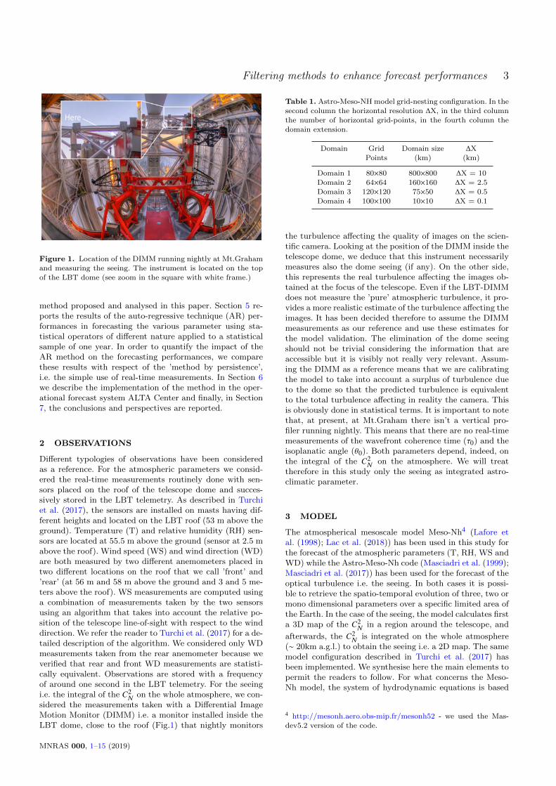
Figure 1. Location of the DIMM running nightly at Mt.Graham

and measuring the seeing. The instrument is located on the top

of the LBT dome (see zoom in the square with white frame.)

method proposed and analysed in this paper. Section 5 re-ports the results of the auto-regressive technique (AR) per-formances in forecasting the various parameter using sta-tistical operators of different nature applied to a statisticalsample of one year. In order to quantify the impact of theAR method on the forecasting performances, we comparethese results with respect of the ’method by persistence’,i.e. the simple use of real-time measurements. In Section 6we describe the implementation of the method in the oper-ational forecast system ALTA Center and finally, in Section7, the conclusions and perspectives are reported.

2 OBSERVATIONS

Different typologies of observations have been consideredas a reference. For the atmospheric parameters we consid-ered the real-time measurements routinely done with sen-sors placed on the roof of the telescope dome and succes-sively stored in the LBT telemetry. As described in Turchiet al. (2017), the sensors are installed on masts having dif-ferent heights and located on the LBT roof (53 m above theground). Temperature (T) and relative humidity (RH) sen-sors are located at 55.5 m above the ground (sensor at 2.5 mabove the roof). Wind speed (WS) and wind direction (WD)are both measured by two different anemometers placed intwo different locations on the roof that we call ’front’ and’rear’ (at 56 m and 58 m above the ground and 3 and 5 me-ters above the roof). WS measurements are computed usinga combination of measurements taken by the two sensorsusing an algorithm that takes into account the relative po-sition of the telescope line-of-sight with respect to the winddirection. We refer the reader to Turchi et al. (2017) for a de-tailed description of the algorithm. We considered only WDmeasurements taken from the rear anemometer because weverified that rear and front WD measurements are statisti-cally equivalent. Observations are stored with a frequencyof around one second in the LBT telemetry. For the seeingi.e. the integral of the C2

N on the whole atmosphere, we con-sidered the measurements taken with a Differential ImageMotion Monitor (DIMM) i.e. a monitor installed inside theLBT dome, close to the roof (Fig.1) that nightly monitors

Table 1. Astro-Meso-NH model grid-nesting configuration. In thesecond column the horizontal resolution ∆X, in the third column

the number of horizontal grid-points, in the fourth column thedomain extension.

Domain Grid Domain size ∆X

Points (km) (km)

Domain 1 80×80 800×800 ∆X = 10

Domain 2 64×64 160×160 ∆X = 2.5Domain 3 120×120 75×50 ∆X = 0.5

Domain 4 100×100 10×10 ∆X = 0.1

the turbulence affecting the quality of images on the scien-tific camera. Looking at the position of the DIMM inside thetelescope dome, we deduce that this instrument necessarilymeasures also the dome seeing (if any). On the other side,this represents the real turbulence affecting the images ob-tained at the focus of the telescope. Even if the LBT-DIMMdoes not measure the ’pure’ atmospheric turbulence, it pro-vides a more realistic estimate of the turbulence affecting theimages. It has been decided therefore to assume the DIMMmeasurements as our reference and use these estimates forthe model validation. The elimination of the dome seeingshould not be trivial considering the information that areaccessible but it is visibly not really very relevant. Assum-ing the DIMM as a reference means that we are calibratingthe model to take into account a surplus of turbulence dueto the dome so that the predicted turbulence is equivalentto the total turbulence affecting in reality the camera. Thisis obviously done in statistical terms. It is important to notethat, at present, at Mt.Graham there isn’t a vertical pro-filer running nightly. This means that there are no real-timemeasurements of the wavefront coherence time (τ0) and theisoplanatic angle (θ0). Both parameters depend, indeed, onthe integral of the C2

N on the atmosphere. We will treattherefore in this study only the seeing as integrated astro-climatic parameter.

3 MODEL

The atmospherical mesoscale model Meso-Nh4 (Lafore etal. (1998); Lac et al. (2018)) has been used in this study forthe forecast of the atmospheric parameters (T, RH, WS andWD) while the Astro-Meso-Nh code (Masciadri et al. (1999);Masciadri et al. (2017)) has been used for the forecast of theoptical turbulence i.e. the seeing. In both cases it is possi-ble to retrieve the spatio-temporal evolution of three, two ormono dimensional parameters over a specific limited area ofthe Earth. In the case of the seeing, the model calculates firsta 3D map of the C2

N in a region around the telescope, and

afterwards, the C2N is integrated on the whole atmosphere

(∼ 20km a.g.l.) to obtain the seeing i.e. a 2D map. The samemodel configuration described in Turchi et al. (2017) hasbeen implemented. We synthesise here the main elements topermit the readers to follow. For what concerns the Meso-Nh model, the system of hydrodynamic equations is based

4 http://mesonh.aero.obs-mip.fr/mesonh52 - we used the Mas-

dev5.2 version of the code.

MNRAS 000, 1–15 (2019)

4 E.Masciadri et al.

Figure 2. Left: temporal evolution of the forecast of the temperature for the whole night (2019/05/17) at Mt.Graham. The forecast

is available at 14:00 UT of the day before. On the x-axes is reported the time expressed in UT (bottom) and local time (top). Right:

temporal evolution of the forecast of the temperature available at 14:00 UT of the day before (black line); real-time measurements insitu (green-line); forecast of the temperature using the AR technique (red line). The latter is calculated at 04:00 UT and extended on

the successive four hours (see text).

Figure 3. Temporal sequence of the up-dated forecasts of the temperature with one hour step during the night 2019/05/17. First image

on top-left is the situation at 04:00 UT of 2019/05/17, last image on bottom right is the situation at 12:00 UT of 2019/05/17. Thesequence is read by rows, from the left to the right. The black line is the forecast of the temperature available at 14:00 LT of the daybefore. It is therefore always the same in all the pictures. The green-line is the real-time measurements. In each picture the end of thegreen line ends at the time in which the AR forecast is calculated. The red-line is the forecast of the temperature obtained with the ARtechnique. The red line in the last picture (bottom-right) represents the model forecast at 1h for the whole night.

MNRAS 000, 1–15 (2019)

Filtering methods to enhance forecast performances 5

upon an anelastic formulation that permits an effective fil-tering of acoustic waves. The model uses the Gal-Chen &Sommerville (1975) coordinates system on the vertical andthe C-grid in the formulation of Arakawa & Messinger (1976)for the spatial digitalization. In this study, we used in thewind advection scheme the ’forward-in-time’ (FIT) numer-ical integrator instead of the’ leap-frog’ one. Such a solu-tion allows for longer time steps and therefore shorter com-puting time. The model employs a one-dimensional 1.5 tur-bulence closure scheme (Cuxart, Bougeault & Redelsperger2000) and we used a one-dimensional mixing length pro-posed by Bougeault & Lacarrere (1989). The surface ex-changes are computed using the interaction soil biosphereatmosphere (ISBA) module (Noilhan & Planton 1989). Theseeing (ε) is calculated with the Astro-Meso-Nh code devel-oped by Masciadri et al. (1999) and since there in continuousdevelopment by our group. The geographic coordinates ofMt.Graham are (32.70131, -109.88906) and the height of thesummit is 3221 m above the sea level. We used a grid-nestingtechnique (Stein et al. 2000) consisting in using different em-bedded domains of the digital elevation models (DEM i.e.orography) extended on smaller and smaller surfaces, withprogressively higher horizontal resolution but with the samevertical grid. Simulations of the OT are performed on threeembedded domains centered on the summit where the hor-izontal resolution of the innermost domain is ∆X = 500 m(Table 1). We used four domains and a highest resolutionof 100 m (Table 1) for the WS because such a configura-tion better reconstructs the WS close to the surface whenthe WS is strong. The model is initialised with analyses pro-vided by the General Circulation Model (GCM) HRES of theEuropean Center for Medium Weather Forecast (ECMWF)having an intrinsic horizontal resolution of around 9 km. Allsimulations we performed with Astro-Meso-Nh start at 00:00UT of the day J and we simulate in total 15 hours5. We con-sider data starting from the sunset up to the sunrise. Duringthe 15 hours the model is forced each six hours (synoptichours) with the forecasts provided by the GCM related tothe correspondent hours. We consider the C2

N outputs witha temporal frequency of two minutes. All the other atmo-spheric parameters have a temporal frequency of the orderof the second. In all cases the simulated data are extractedfrom the innermost domain (domain 3 or 4 - see discussionon the wind speed a few line above). We have a 54 verticallevels with a first grid point of 20 m, a logarithmic stretchingof 20 per cent up to 3.5 km above the ground and almostconstant vertical grid size of ∼600 m up to 23.57 km. Theheight of the first grid point has been fixed to be able toresolve the in-situ measurements of the various parametersanalysed in this study.

5 To avoid misunderstandings found in the literature, we high-light that a simulation of 15h does not mean that we need 15h

to simulate that period. It means that we reconstruct the atmo-

spheric evolution of 15h. The simulated time and the effectivecalculation time required to perform a calculation are two differ-

ent concepts of ’time’.

4 AUTOREGRESSIVE METHOD

As we said in Section 1, the goal of this study is to verifyif we can improve the model performances of forecasts ontime scales of a few hours. The method that we propose touse in this paper is based on the auto-regressive (AR) tech-nique. We chose a formulation inspired by Dzhaparidze etal. (1994). The method is based on a function that dependson the difference between the real-time observations takenin-situ that we take as a reference (i.e. we assume to be the”truth”) and on the forecasts performed by the atmosphericmodel. When we deal about ’atmospherical model’ we arereferring to the forecast of the model in standard configura-tion (see Section 3) that is available early in the afternoonof the day before6. The auto-regressive model (AR) X∗

t+1calculated at the (t + 1) is:

X∗t+1 = Mt+1 + Xt+1 (1)

where M is the model output at the time (t +1) and the func-tion X at the time (t + 1) depends on the difference betweenthe observations and the atmospherical model outputs cal-culated on a polinomial function built with the addition ofP terms characterised by P coefficient ai (called regressors)in the form:

Xt+1 =P∑i=1

ai(OBSt−i+1 − MODt−i+1). (2)

where the variable OBS indicates the real-time measure-ments and MOD the atmospheric model outputs in the stan-dard configuration. From one side, the larger is P, the largeris the number of the regressors, the more accurate is thefit to the trend of the past observations. On the other side,we have interest in limiting the number of the coefficientsai to limit the computation time. We identified an optimaltrade-off P=50 for a temporal frequency of 1 minute.

The values of the 50 regressors is obtained through aLeast Mean Square (LSM) method applied to a finite num-ber of nights in the past i.e., for example, the last 3, 4, 5,etc. nights.

Figure 2 shows how the AR method works. The pictureshows, as an example, the forecast of the temperature butthe same procedure can be used for whatever parameter.On the left side is shown the standard forecast of the night2019/05/177 that is available early in the afternoon. On theright side is reported an example of the AR method appliedat 04:00 UT. The black line is the standard forecast withthe atmospheric model (same as the left side), the greenline represents the real-time measurements up to 04:00 UT(that is the present time), the red line represent the forecastcalculated at 04:00 UT with the AR method for the suc-cessive 4 hours. As we are interested here on studying theforecast performances on time scales of one or two hours,we considered therefore a AR forecast of 4 hours that cer-tainly covers this time scale. We expect that the effect of

6 For simplicity, we will call hereafter simply ’model’ the Meso-

Nh or the Astro-Meso-Nh models, knowing that the first one isused for the atmospheric parameters, the second one for the OT.7 The date refers to the start of the night.

MNRAS 000, 1–15 (2019)

6 E.Masciadri et al.

the data-assimilation of the local measurements provides animprovement of the forecast that is maximum close to thepresent time (nowcasting) and it decreases with the time upto disappear. The positive effect of the AR method vanishesafter a ∆T that is when the performance of the AR methodis equal to the performance of the atmospheric model instandard configuration. Later on, in Section 5, this aspectwill be treated in a more detailed way. If the same proceduredescribed in Fig. 2 is repeated with the suitable frequencyduring the whole night, it is possible to obtain a forecast ona time scale of one hour.

Figure 3 reports the sequence of successive AR forecaststhat are recalculated at each full hour during the night. Thesequence has to be read from the top to the bottom, fromthe left to the right, following the different rows. We observethat, in each successive picture of the sequence, the greenline becomes longer of one hour and the red-line, showingthe forecast related to the successive four hours, shifts ofone hour on the right. If we consider the red line of thelast picture (bottom-right) extended on the whole night, wehave the performance of the system on a time scale of onehour. We highlight that, in this computation and procedure,we take into account only data between the sunset and thesunrise.

As said previously, the unique free parameter remainsthe number of nights (N) on the past on which to calculatethe values of the regressors. As we will see later on, N=5 isa suitable number for our application. The whole analysispresented in Section 5 has been performed assuming thisvalue for N.

5 RESULTS

In order to quantify the model performances of the forecastson one hour time scale using the AR method built as de-scribed in Section 4 it is necessary to consider a very rich sta-tistical sample because the AR method requires a sequenceof observed data related to successive nights in which it isimportant to minimise the number of breaks (lack of mea-surements). We considered therefore data of all the nights ofthe whole year 2018 and we calculated the statistical opera-tors (bias, RMSE and σ)8 for temperature, relative humid-ity, wind speed, wind direction and the total seeing. Real-time measurements and outputs of the atmospheric modelin standard-configuration related to these parameters havebeen treated using the same procedure: we first apply a mov-ing average of one hour to filter out the high frequencies andput in evidence the forecast trend, we perform a resamplingon a time scale of 20 minutes9 and we conclude with thecalculation of the various statistical operators.

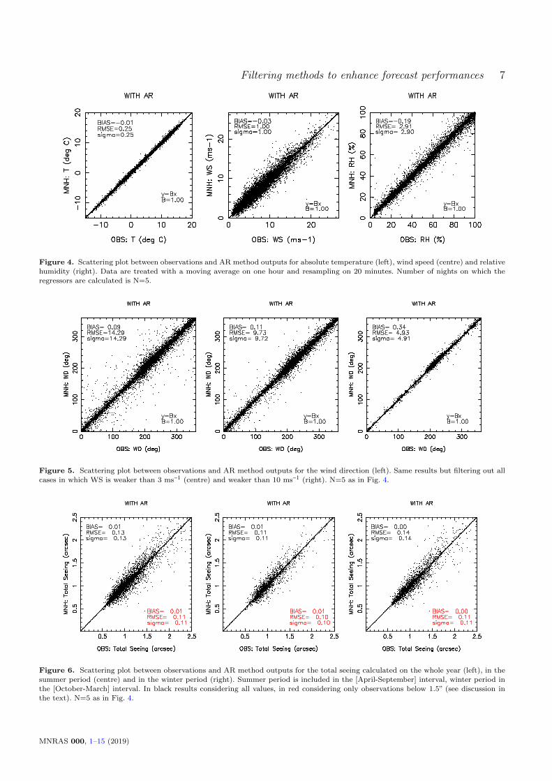
Figure 4 shows the scattering plot related to the tem-perature (left), the wind speed (centre) and the relative hu-midity (right) obtained with an AR at a time scale of 1 hour.Figure 5 shows the scattering plot of the WD at the sametime scale of 1 hour obtained including all the data (left), fil-tering out all the data associated to wind speed weaker than3 ms−1 (centre) and filtering out all data having a wind speed

8 We refer the reader to Masciadri et al. (2017) for the definitionof the statistical operators.9 A resampling on 10 minutes provide a very similar result.

weaker than 10 ms−1. We skipped out the data associatedto a WS weaker than 3 ms−1 because under this conditionit is extremely difficult (and meaningless) to quantify theWD because of the high variability of the WD. The centralpicture of Fig.5 is therefore more representative for the WDthan the left one. We skipped-out data weaker than 10 ms−1

to quantify the model performances in those cases that arecertainly the most critical one for the ground-based observa-tions, i.e. those in which the WS is very strong. To conclude,Fig. 6 shows the scattering plot for the seeing in the wholeyear (left), in the summer [April - September] interval (cen-tre) and winter [October - March] interval (right).

Table 2 reports the RMSE obtained for the AR methodat a time scale of 1 hour and with the atmospheric model inthe standard configuration. As we observe that, in the stan-dard configuration10, the dispersion of the seeing increasesfor large seeing values but the forecasts are less interestingfor those cases. We decided, therefore, to consider observa-tions below 1.5”. From a practical point of view, indeed, inthe astronomical context it is poorly interesting to discrimi-nate seeing values between 1.5” and larger values. We main-tained both cases for the AR (Fig.6) because the RMSE arevery similar. We observe that, for all the parameters, the val-ues of RMSE obtained with the AR method at a time scaleof 1h are definitely better than for the standard configura-tion with consistent gains that are variable depending on theparameters between a minimum of a factor 2.7 and a max-imum of 4.9 (Table 3-first row). Those gains are definitelyconsistent and, at our knowledge, these model performanceshave never been achieved before. In Annex A is reported adetailed description on the number of nights used to analysethis statistics for each parameter. The extremely small valueof the RMSE for the temperature of the order of 0.25◦ tellsus that, with such performances in predicting the tempera-ture close to the ground, the elimination of the dome seeingthrough a thermalisation of the primary mirror temperatureand the atmosphere inside the dome with respect to the ex-ternal temperature is not a dream anymore, as declared byRacine et al. (1991).

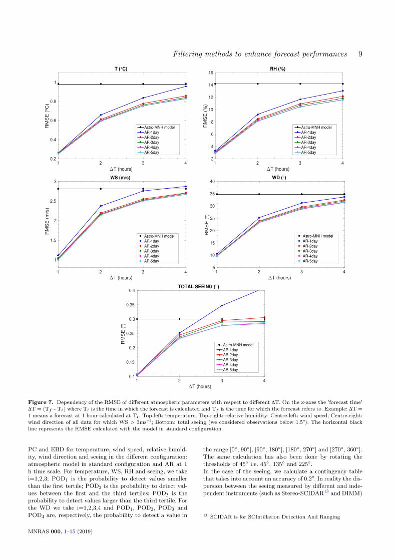
It remains to consider how to fix the number of nightson which to calculate the regressors. Figure 7 shows howthe RMSE obtained with the AR method changes as afunction of the interval of time ∆T on which we calculatethe forecast and as a function of N. We decided to consider∆T = 1 hour as a minimum value because, consideringthe logistic requiring a change of program or the set-up ofan instrument, makes poorly interesting to go below thisthreshold. As expected, the gain is maximum at 1h and itdecreases as ∆T increases11. The black line, represents, foreach parameters, the RMSE obtained with atmosphericalmodel in standard configuration that is obviously constantfor the whole night. We note that there is a saturationeffect for N equal to 4 or 5. We decided therefore to useN=5 in our calculation because no further gain is visiblefor N larger than 5. The point in which coloured lines crossthe black line represents the ∆T at which the AR stops topresent an improvement in the performances with respect

10 This feature has not been observed after the application of theAR technique as one can see in Fig.611 When ∆T = 0 we have the nowcasting.

MNRAS 000, 1–15 (2019)

Filtering methods to enhance forecast performances 7

Figure 4. Scattering plot between observations and AR method outputs for absolute temperature (left), wind speed (centre) and relative

humidity (right). Data are treated with a moving average on one hour and resampling on 20 minutes. Number of nights on which the

regressors are calculated is N=5.

Figure 5. Scattering plot between observations and AR method outputs for the wind direction (left). Same results but filtering out allcases in which WS is weaker than 3 ms−1 (centre) and weaker than 10 ms−1 (right). N=5 as in Fig. 4.

Figure 6. Scattering plot between observations and AR method outputs for the total seeing calculated on the whole year (left), in the

summer period (centre) and in the winter period (right). Summer period is included in the [April-September] interval, winter period inthe [October-March] interval. In black results considering all values, in red considering only observations below 1.5” (see discussion inthe text). N=5 as in Fig. 4.

MNRAS 000, 1–15 (2019)

8 E.Masciadri et al.

Table 2. RMSE as obtained with the atmospheric model in the standard configuration and as obtained with the AR method on a1h time scale. In the case of the seeing we considered only seeing below 1.5”. This threshold is more than representative for the AO

applications and it guarantees a model performances comparable to the dispersion obtained with measurements.

RMSE T RH WS WD (> 3ms−1) Seeing

(◦ K) (%) (ms−1) (degrees) (arcsec)

atm. model standard config. 0.98 14.17 2.81 34.71 0.30

AR (@ 1h) 0.25 2.91 1.00 9.73 0.11

Table 3. First row: gain obtained for the RMSE for the different

atmospheric and astroclimatic parameters of the AR method ona time scale of 1h with respect to the model standard configu-

ration. Second row: gain using the method by persistence on the

same time scale with respect to the model standard configuration.Third row: gain of the AR method with respect to the method

by persistence on the same time scale.

GAIN T RH WS WD Seeing

AR 3.90 4.90 2.80 3.60 2.70Persistence 2.40 3.00 1.80 2.40 2.00

AR / Persistence 1.63 1.63 1.56 1.50 1.35

Table 4. Climatology tertiles calculated on measurements ex-tended on one full solar year (2018) for the absolute temperature

T, the wind speed WS, the relative humidity RH and the seeing.

Param. 1st tert. Median 3rd ter.

T (◦) 1.00 4.11 8.23

WS (ms−1) 5.52 7.15 9.08

RH (%) 31.63 47.48 66.67

seeing (”) 0.93 1.05 1.20seeing (< 1.5”) 0.90 0.99 1.10

to the standard configuration and it starts to diverge. For∆T larger than this threshold, the standard configurationis more advantageous than the AR method. This is exactlythe expected trend as the in-situ measurements stop tohave a positive influence on the forecast performances for∆T too large. We can observe that, the AR continues tomaintain a gain different from zero up to a time scale of theorder of 4-6 hours12.

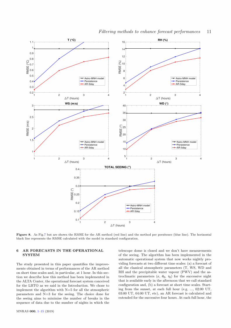
Once analysed the gain obtained employing the auto-regression approach, it might be interesting to quantifywhich is the gain on a time scale of a few hours if weuse just real-time measurements instead of the filteringtechniques. We call this approach ’method by persistence’.This means that, at each full hour, the forecast extendedon the successive 4 hours, is obtained by considering thepresent time measurements as a constant for all its futureevolution. Fig.8 shows the RMSE versus the ∆T obtained

12 The reason why we display the figure only up to 4 hours is to

avoid a too large inhomogeneity in the statistical representativityof the samples. The number of samples for each ∆T decreases

indeed, as we increase ∆T.

with the optmized AR method (N=5) and the persistencemethod. It is clearly visibly that, as expected, even if the useof pure real-time measurements provides an improvement ofthe forecast performances on short time scales with respectto the standard configuration of the model, the AR methodthat we propose has definitely a more important gain andbetter performances for all the atmospheric parametersincluding the optical turbulence with differences (withrespect to the persitence method) that are quantitativelynot negligible. Table 3-second row reports the gain of thepersistence method with respect to the model forecast instandard configuration. Table 3-third row reports the gainof the AR method with respect to the persistence method.Looking at Fig.8 it is also possible to observe that, in thecase of the AR method, the gain persists for a much longer∆T with respect to the persistence approach. It is worth tonote that, of course, the black line of the model forecast instandard configuration is available much earlier than thestart of the observing night. It is therefore obviously worsewith respect to the other two methods. The fair comparisonis therefore between the red and the blue lines.

To complete the analysis of the model performances,we finally calculate the contingency tables for each param-eter from which we can retrieve the probability of detec-tion (POD), the percentage of correct detection (PC) andthe extremely bad detection (EBD). Contingency tables al-low for the analysis of the relationship between two or morecategorical variables.We refer the readers to Lascaux et al.(2015) for a detailed definition and description of this tool.To permit the readers to follow the text we refer to Annex Bthat contains a synthesis of the definitions of the statisticaloperators. Here we just remind the principal role of the con-tingency tables. Given a statistical sample of observationsand predictions, the contingency tables permit to calculatethe number of times in which observations and predictionsfall in the same intervals of values. We used 3×3 tables forall the parameters with exception of the WD that requiresa 4×4 table as it is a 2π periodic parameter. Starting fromthis distribution it is possible to calculate the probability todetect a specific atmospheric parameter in specific intervalsof values, the so called PODi , the percentage of correct de-tection (PC) and the extremely bad detection (EBD). Thethresholds of the intervals are calculated from the clima-tology of in-situ measurements and they are, usually, thefirst and third tertiles of the cumulative distribution. Table4 reports the first and third tertiles calculated on one year(2018) of measurements for the different atmospheric pa-rameters. These values are used as thresholds in this study.Table 5, 6, 7, 8, 9 and Table 10 report the results of PODi ,

MNRAS 000, 1–15 (2019)

Filtering methods to enhance forecast performances 9

1 2 3 4

T (hours)

0.2

0.4

0.6

0.8

1

RM

SE

(°C

)

T (°C)

Astro-MNH model

AR-1day

AR-2day

AR-3day

AR-4day

AR-5day

1 2 3 4

T (hours)

2

4

6

8

10

12

14

16

RM

SE

(%

)

RH (%)

Astro-MNH model

AR-1day

AR-2day

AR-3day

AR-4day

AR-5day

1 2 3 4

T (hours)

1

1.5

2

2.5

3

RM

SE

(m

/s)

WS (m/s)

Astro-MNH model

AR-1day

AR-2day

AR-3day

AR-4day

AR-5day

1 2 3 4

T (hours)

5

10

15

20

25

30

35

40

RM

SE

(°)

WD (°)

Astro-MNH model

AR-1day

AR-2day

AR-3day

AR-4day

AR-5day

1 2 3 4

T (hours)

0.1

0.15

0.2

0.25

0.3

0.35

0.4

RM

SE

(")

TOTAL SEEING (")

Astro-MNH model

AR-1day

AR-2day

AR-3day

AR-4day

AR-5day

Figure 7. Dependency of the RMSE of different atmospheric parameters with respect to different ∆T. On the x-axes the ’forecast time’∆T = (T f - Ti) where Ti is the time in which the forecast is calculated and T f is the time for which the forecast refers to. Example: ∆T =

1 means a forecast at 1 hour calculated at Ti . Top-left: temperature; Top-right: relative humidity; Centre-left: wind speed; Centre-right:wind direction of all data for which WS > 3ms−1; Bottom: total seeing (we considered observations below 1.5”). The horizontal black

line represents the RMSE calculated with the model in standard configuration.

PC and EBD for temperature, wind speed, relative humid-ity, wind direction and seeing in the different configuration:atmospheric model in standard configuration and AR at 1h time scale. For temperature, WS, RH and seeing, we takei=1,2,3; POD1 is the probability to detect values smallerthan the first tertile; POD2 is the probability to detect val-ues between the first and the third tertiles; POD3 is theprobability to detect values larger than the third tertile. Forthe WD we take i=1,2,3,4 and POD1, POD2, POD3 andPOD4 are, respectively, the probability to detect a value in

the range [0◦, 90◦], [90◦, 180◦], [180◦, 270◦] and [270◦, 360◦].The same calculation has also been done by rotating thethresholds of 45◦ i.e. 45◦, 135◦ and 225◦.In the case of the seeing, we calculate a contingency tablethat takes into account an accuracy of 0.2”. In reality the dis-persion between the seeing measured by different and inde-pendent instruments (such as Stereo-SCIDAR13 and DIMM)

13 SCIDAR is for SCIntillation Detection And Ranging

MNRAS 000, 1–15 (2019)

10 E.Masciadri et al.

can reach values as high as 0.29” Masciadri et al. (2019) butwe decided to use 0.2” to be more conservative and becausethis is a technical specification assumed in some top-classtelescopes.

We observe that, for the AR forecasts at 1h, in the caseof temperature, RH, WD and seeing, almost all the PODi

are very close to the saturation (values in the [94%, 99%]range) i.e. with small space for further improvements. ThePC is also of the same order of magnitude and the EBDbasically equal to zero. The wind speed is still very good,only POD2 = 83% but the most important ones (POD1 andPOD3) i.e. the probability to detect extremely weak andthe extremely strong wind speed are > 90%. This tool mighttherefore be extremely important to face the so called ”lowwind effect” i.e. a significant deterioration of image qualityobserved with high contrast imaging instruments such asSPHERE14 (Milli et al. 2018) when the wind speed is low orabsent. This condition enhances the radiative cooling of thespiders that obstruct the big telescopes pupil, creating airtemperature inhomogeneities on the phase across the pupil.For WS ≤ 4ms−1 we calculated that the model is able to re-construct the WS with an RMSE=0.7ms−1. On the other ex-treme, we calculated that, for WS ≥ 10 ms−1, the model wellreconstructs the WS with a RMSE=1.2 ms−1. This meansthat the method is extremely efficient in predicting the con-ditions of strong wind speed that represent the main causeof vibration of the adaptive secondaries and/or the primarymirrors.

Looking at the same Tables 5, 6, 7, 8, 9 and Table 10,we observe that performances of the atmospherical model instandard configuration are weaker than those of the AR at1h as expected, but still very good. We do not comment fur-ther results found in this configuration for the atmosphericparameters as a precedent paper has been dedicated to thisaspect Turchi et al. (2017). This calculation has been re-peated here (with the same statistical sample used for theAR method at 1h) to be able to quantify the improvementin terms of model performances on short time scales. Thenew result of this paper is however the estimate of statis-tical operators (PODi , PC and EBD) for the seeing (Table10-second column) that reveals to be very promising i.e. allthe PODi are of the order of 97-98%.

We put the accent on the most relevant result obtainedin this analysis and related to the seeing. The most criticalPOD1 i.e. the probability to detect a seeing weaker than thefirst tertile is equal to 81% for the standard configurationand it is equal to 98% for the AR method at 1h time step.Both are well above the threshold of 33% that is the per-centage that corresponds to the random case and the ARmethod is very close to the saturation in terms of perfor-mances. Somehow weaker is the probability to detect theseeing larger than the third tertile (65%) in the standardconfiguration as the larger is the seeing, the larger is thedispersion between observations and numerical calculation.We have here more space for further improvements of thetechnique.

14 High contrast imaging of the Very Large Telescope located at

foci of UT3.

Table 5. Model performances in reconstructing the absolutetemperature at different time scales: at 14h i.e. when we provide

a forecast early in the afternoon of the day (J-1) for the next night,

and at 1h with AR. POD1, POD2 and POD3 are the probabilityof detection related to the intervals: T < 1st tertile, 1st tertile

< T < 3r d tertile, T > 3r d tertile. The 1st and tertiles 3r d are

shown in Table 4.

Temperature (T)

Param. Forecast Forecast with AR

the day before (%) @ 1h (%)

POD1 96 99

POD2 91 98

POD3 96 99PC 94 99

EBD 0 0

Table 6. As Table 5 but for the wind speed (WS).

Wind Speed (WS)

Param. Forecast Forecast with AR

the day before (%) @ 1h (%)

POD1 72 91

POD2 48 83

POD3 75 93PC 65 89

EBD 2 0

Table 7. As Table 5 but for the relative humidity (RH).

Relative Humidity (RH)

Param. Forecast Forecast with AR

the day before (%) @ 1h (%)

POD1 91 98POD2 73 95POD3 71 97

PC 78 97

EBD 1 0

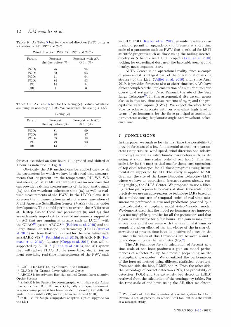
Table 8. As Table 5 but for the wind direction (WD) using asa thresholds: 90◦, 180◦ and 270◦.

Wind direction (WD: 90◦, 180◦ and 270◦)

Param. Forecast Forecast with AR

the day before (%) @ 1h (%)

POD1 78 94

POD2 75 93POD3 88 94

POD4 57 93

PC 81 94EBD 2 0

MNRAS 000, 1–15 (2019)

Filtering methods to enhance forecast performances 11

1 2 3 4

T (hours)

0.2

0.3

0.4

0.5

0.6

0.7

0.8

0.9

1

1.1

RM

SE

(°C

)

T (°C)

Astro-MNH model

Persistence

AR-5day

1 2 3 4

T (hours)

2

4

6

8

10

12

14

16

RM

SE

(%

)

RH (%)

Astro-MNH model

Persistence

AR-5day

1 2 3 4

T (hours)

1

1.5

2

2.5

3

RM

SE

(m

/s)

WS (m/s)

Astro-MNH model

Persistence

AR-5day

1 2 3 4

T (hours)

5

10

15

20

25

30

35

40

RM

SE

(°)

WD (°)

Astro-MNH model

Persistence

AR-5day

1 2 3 4

T (hours)

0.1

0.15

0.2

0.25

0.3

0.35

0.4

RM

SE

(")

TOTAL SEEING (")

Astro-MNH model

Persistence

AR-5day

Figure 8. As Fig.7 but are shown the RMSE for the AR method (red line) and the method per persitence (blue line). The horizontal

black line represents the RMSE calculated with the model in standard configuration.

6 AR FORECASTS IN THE OPERATIONALSYSTEM

The study presented in this paper quantifies the improve-ments obtained in terms of performances of the AR methodon short time scales and, in particular, at 1 hour. In this sec-tion we describe how this method has been implemented inthe ALTA Center, the operational forecast system conceivedfor the LBTO as we said in the Introduction. We chose toimplement the algorithm with N=5 for all the atmosphericparameters and N=3 for the seeing. The choice done forthe seeing aims to minimise the number of breaks in thesequence of data due to the number of nights in which the

telescope dome is closed and we don’t have measurementsof the seeing. The algorithm has been implemented in theautomatic operational system that now works nightly pro-viding forecasts at two different time scales: (a) a forecast ofall the classical atmospheric parameters (T, WS, WD andRH and the precipitable water vapour (PWV) and the as-troclimatic parameters (ε, θ0, τ0) for the successive nightthat is available early in the afternoon that we call standardconfiguration and, (b) a forecast at short time scales. Start-ing from the sunset, at each full hour (e.g. ..., 02:00 UT,03:00 UT, 04:00 UT, etc), an AR forecast is calculated andextended for the successive four hours. At each full hour, the

MNRAS 000, 1–15 (2019)

12 E.Masciadri et al.

Table 9. As Table 5 but for the wind direction (WD) using as

a thresholds: 45◦, 135◦ and 225◦.

Wind direction (WD: 45◦, 135◦ and 225◦)

Param. Forecast Forecast with AR

the day before (%) @ 1h (%)

POD1 75 94

POD2 62 93POD3 71 94

POD4 84 93

PC 74 94EBD 1 0

Table 10. As Table 5 but for the seeing (ε). Values calculatedassuming an accuracy of 0.2”. We considered the seeing < 1.5”.

Seeing (ε)

Param. Forecast Forecast with AR

the day before (%) @ 1h (%)

POD1 81 99

POD2 80 97

POD3 65 98PC 79 98

EBD 14 1

forecast extended on four hours is upgraded and shifted of1 hour as indicated in Fig. 3.

Obviously the AR method can be applied only to allthe parameters for which we have in-situ real-time measure-ments that, at present, are the temperature, RH, WS, WDand seeing. So far at Mt.Graham there are no monitors thatcan provide real-time measurements of the isoplanatic angle(θ0) and the wavefront coherence time (τ0) as well as real-time measurements of the PWV. In the LBTO plans, it isforeseen the implementation in situ of a new generation ofMulti Aperture Scintillation Sensor (MASS) that is underdevelopment. This should permit to extend the AR forecastat 1h step also to these two parameters (θ0 and τ0) thatare extremely important for a set of instruments supportedby AO that are running at present such as LUCI15 withthe GLAO16 system ARGOS17 (Rabien et al. 2019) and theLarge Binocular Telescope Interferometry (LBTI) (Hinz etal. 2016) or those that are planned for the near future suchas SHARK-VIS18 (Pedichini et al. 2016), SHARK-NIR (Far-inato et al. 2018), iLocator (Crepp et al. 2016) that will besupported by SOUL19 (Pinna et al. 2016), the AO systemthat will replace FLAO. At the same time, also an instru-ment providing real-time measurements of the PWV such

15 LUCI is for LBT Utility Camera in the Infrared16 GLAO is for Ground Layer Adaptive Optics17 ARGOS is for Advance Rayleigh guided Ground layer adaptive

Optics System18 SHARK is for System for coronography with High order Adap-

tive optics from R to K bands. Originally a unique instrument,in a successive phase it has been decided to develop two differentunits in the visible (VIS) and in the near-infrared (NIR).19 SOUL is for Single conjugated adaptive Optics Upgrade for

the LBT

as LHATPRO (Kerber et al. 2012) is under evaluation asit should permit an upgrade of the forecasts at short timescale of a parameter such as PWV that is critical for LBTIscientific programs such as those using the nulling interfer-ometry in N band - see HOST project (Ertel et al. 2018)looking for exozodiacal dust near the habitable zone aroundnearby, main-sequence stars.

ALTA Center is an operational reality since a coupleof years and it is integral part of the operational observingstrategy of the LBT (Veillet et al. 2016) and, since April2019, it provides forecasts also at short time scale. We havealmost completed the implementation of a similar automaticoperational system for Cerro Paranal, the site of the VeryLarge Telescope20. In this astronomical site we can accessalso to in-situ real-time measurements of θ0, τ0 and the pre-cipitable water vapour (PWV). We expect therefore to beable to achieve forecasts with an equivalent high level interms of performances for the three principal astroclimaticparameters: seeing, isoplanatic angle and wavefront coher-ence time.

7 CONCLUSIONS

In this paper we analyse for the first time the possibility toprovide forecasts of a few fundamental atmospheric param-eters (temperature, wind speed, wind direction and relativehumidity) as well as astroclimatic parameters such as theseeing at short time scales (order of one hour). This timescale is by far the most critical one for the science operationsof top-class telescopes for all those programs using instru-mentation supported by AO. The study is applied to Mt.Graham, the site of the Large Binocular Telescope (LBT)where we have an operational forecast system already run-ning nightly, the ALTA Center. We proposed to use a filter-ing technique to provide forecasts at short time scale, moreprecisely we use an auto-regressive technique (AR) based onthe simultaneous use of temporal series of real-time mea-surements performed in situ and predictions provided by anon-hydrostatic atmospheric model Astro-Meso-Nh model.We demonstrated that the model performances are improvedby a not negligible quantities for all the parameters and thata gain is still visible for a few hours. The gain is maximumat one hour and it decreases with the time until it vanishescompletely when effect of the knowledge of the in-situ ob-servations at present time loose its positive influence on thefuture. The values of this thresholds are between 4 and 6hours, depending on the parameter (Fig.7).

The AR technique for the calculation of forecast at atime scale of one hour produces a gain on model perfor-mances of a factor 2.7 up to almost 5 (depending on theatmospheric parameter). We quantified the performancesof the forecast method using different statistical operators.From one side the bias, RMSE and σ. From the other side,the percentage of correct detection (PC), the probability ofdetection (POD) and the extremely bad detection (EBD)retrieved from the calculation of the contingency tables. Forthe time scale of one hour, using the AR filter we obtain:

20 We point out that the operational forecast system for CerroParanal is not, at present, an official ESO tool but it is the resultof a research study.

MNRAS 000, 1–15 (2019)

Filtering methods to enhance forecast performances 13

a RMSE=0.25◦ for the temperature, a RMSE=2.91% forthe relative humidity, a RMSE=1ms−1 for the wind speed,a RMSE=9.73 degrees for the wind direction when we filterout the wind speed weaker than 3ms−1 and a RMSE=0.11”for the seeing.

Looking at the analysis from the point of view of thecontingency tables and probability of detection, we find thatall the PODi are well above 90% reaching in many cases(seeing, temperature, RH and WD) more than 95%. Thiscondition is already very close to the saturation with smallspace for further improvement. The WS also presents ex-cellent performances for the PODi larger than 90%. POD2is slightly weaker (83%) and tells us that is slightly moredifficult to discriminate between the first tertile (5.52 ms−1)and the third tertile (9.98 ms−1). Besides that, the system isextremely efficient in predicting the weak wind speed (witha RMSE=0.7ms−1) and in predicting the very strong windspeed (with a RMSE=1.2ms−1), that makes the tool veryuseful to face the low wind effect in high contrast imaginginstruments (see Section 5) and to identify the interval oftime characterised by very strong wind (WS > 10ms−1).

Results obtained for the optical turbulence, and moreprecisely with the seeing, are extremely satisfactory. Weproved that the AR technique allows us to reach a RMSE ofthe order of 0.11” at 1 hour and PODi of the order of 98%.The most relevant result obtained in this study is definitelyrelated to the seeing. The most critical POD1 i.e. the proba-bility to detect a seeing weaker than the first tertile is equalto 81% for the standard configuration and it is equal to 98%for the AR method at 1h time step. This definitely repre-sents a fundamental milestone for the implementation of theflexible-scheduling of ground-based top-class telescopes.

Besides that, we quantified the gain obtained by the ARapproach with respect to the use of pure real-time measure-ments i.e. the persistence method putting in evidence thatthe percentage of RMSE gain is between 35% and 63% andit is therefore far from being negligible.

Once validated, we implemented this method in the au-tomatic and operational forecast system conceived for theLBTO named ALTA Center. The outputs of such a forecastsystem are currently automatically injected into the softwaredriving the science operations at the LBTO. At our knowl-edge, this is the first automatic operational system providingthis kind of information, at least in the astronomical context.

We are implementing a similar automatic and opera-tional system for the VLT and, in this case, we will be ableto predict at short time scales, also the isoplanatic angle andthe wavefront coherence time thanks to the presence of in-strument providing real-time measurements of these param-eters. It will be interesting to quantify the performances ofthis method on different sites. We point out that, at present,this is not an official operational ESO tool.

In terms of filtering techniques, it is our intention to re-fine our results to evaluate if other methods such as Kalmanor machine learning, and multiple ways to use them, mightprovide supplementary improvements of the technique.

ACKNOWLEDGEMENTS

This work is funded by the contract ENV001 (LBTO). Theauthors acknowledge the LBTO Director, Christian Veillet

and the LBT Board for supporting them in the developmentof the ALTA Center. The authors thanks the LBTO staff,and in particular Matthieu Bec, for their collaboration inkeeping synchronised the real-time LBT telemetry and theALTA Center. The authors thanks the Meso-Nh users sup-porter team who constantly works to maintain the modelby developping new packages in progressing model versions.Initialisation data come from the GCM of the ECMWF.

REFERENCES

Arakawa A. & Messinger F., 1976, GARP Tech. Rep., 17,

WMO/ICSU, Geneva, Switzerland

Bougeault, P. & Lacarrere, P., 1989, Mon. Weather. Rev., 117,

1972

Cherubini, T., Businger, S., Lymann, R, Chun, M., 2008, J. Appl.

Meteorol. and Climatology, 47, 1140

Cherubini, T., Businger, S., Lyman, R., 2011, Optical Turbulence

- Astronomy meets Meteorology, pp. 196, Edit. Masciadri &Sarazin, Imperial College Press

Crepp, J., Crass, J., King, D., et al., 2016, Proc. SPIE 9908,

Ground-based and Airborne Instrumentation for Astronomy

VI, 990819

Cuxart, J., Bougeault, P., Redelsperger, J.-L., 2000, Q. J. R. Me-

teorol. Soc., 126, 1

Dzhparidze, K., Kormos, J., Van der Meer, T., Zuijlen, M.C.A.,1994, Math. Comput. Modelling, 19, 29

Ertel, Defrere, D., Hinz, P., et al. 2018, AJ, 155, Issue 5, articleid. 194

Farinato, J., Agapito, G., Bacciotti, F., et al., 2018, Proc. SPIE

10703, Adaptive Optics Systems VI, 107030E

Gal-Chen, T., Sommerville, C. J., 1975, J. Comput. Phys., 17,

209

Giordano, C., Vernin, J., Vazquez-Ramio, H. et al., 2013, MN-

RAS, 430, 3102

Hagelin S., Masciadri E., Lascaux F., 2011, MNRAS, 412, 2695

Hinz, P. et al., 2016, Proc. SPIE 9907, Optical and Infrared In-

terferometry and Imaging V, 990704

Kerber, F., et al., 2012, Proc. SPIE, Ground-based and Airborne

Telescopes IV, 8448, 84463N

Lac, C. et al., 2018, Annales Geosci. Model Dev., 11, 1929

Lafore J.-P., Stein, J., Asencio, N. et al., 1998, Annales Geophys-

icae, 16, 90

Lascaux F., Masciadri E., Fini, L., 2015, MNRAS, 449, 1664

Lascaux F., Masciadri E., Hagelin S., 2011, MNRAS, 411, 693

Lascaux F., Masciadri E., Hagelin S., 2010, MNRAS, 403, 1714

Liu, L.Y., Giordano, C., Yao, T.Q. et al., 2015, MNRAS, 451,3299

Masciadri, E., Turchi, A., Martelloni, G., AO4ELT6, Quebec City,9-14 June 2019, arXiv:1911.02819

Masciadri, E., Lascaux, F., Fini, L., 2017, MNRAS, 466, 520

Masciadri, E., Lascaux, F., Fini, L., 2013, MNRAS, 436, 1968

Masciadri, E. & Egner, S., 2006, PASP, 118, 1604

Masciadri, E., Avila R., Sanchez L.J., 2004, RMxAA, 40, 3

Masciadri, E., Avila, R., Sanchez, L. J., 2002, A&A, 382, 387

Masciadri E. & Jabouille P., 2001, A&A, 376, 727

Masciadri, E., Vernin J., Bougeault P., 1999, A&ASS, 137, 185

Milli, J., Kasper, M., Bourget, P., et al., 2018, Proc. SPIE 10703,Adaptive Optics Systems VI, 107032A

Noilhan J. & Planton S., 1989, Mon. Weather. Rev., 117, 536

Osborn, J. & Sarazin, M., 2018, MNRAS, 480, 1278

Pedichini, F., Ambrosino, F., Centrone, M., et al., 2016, Proc.

SPIE 9908, Ground-based and Airborne Instrumentation forAstronomy VI, 990832

Pinna, E., Esposito, S., Hinz, P, et al., 2016, Proc. SPIE 9909,

Adaptive Optics Systems V, 99093V

MNRAS 000, 1–15 (2019)

14 E.Masciadri et al.

Rabien, S., Angel, R., Barl. L., et al., A&A, 621, A4

Racine, R., 1991, PASP, 103, 1020

Stein J., Richard E., Lafore J.-P. et al., 2000, Meteorol. Atmos.Phys., 72, 203

Trinquet, & Vernin, J., 2007, Environ. Fluid Mech., 7, 397

Turchi, A., Masciadri, E., Kerber, F., Martelloni, G., 2019, MN-RAS, 482, 206

Turchi, A., Martelloni, G., Masciadri, E., 2018, Proc. SPIE, Vol.10703, id. 107036H

Turchi, A., Masciadri, E., Fini, L., 2017, MNRAS, 466, 1925

Veillet, C., Ashby, D.S., Christou, J., et al., 2016, Proc. SPIE9910, Observatory Operations: Stretegies, Processes and Sys-

tems VI, 99100S

Ye, Q.Z., 2011, PASP, 123, 113

Table A1. Number or nights used for the analysis of modelperformances using the AR method. They are extracted from the

sample of 365 nights of 2018.

2018 year T RH WS WD Seeing

Num. of nights 351 351 324 324 229

APPENDIX A: SAMPLE USED FOR THESTATISTICS ANALYSIS

Table A1 summarises the effective number of nights usedfor the analysis for each parameter. For temperature andrelative humidity we have 351 nights i.e. just a few nightshave been missed, for WS and WD we have a total of 324nights and for the seeing we have a total of 229 nights. Thereasons for the missing nights are of different nature. For at-mospheric parameter, the reason is mainly given by sporadicfailure of the sensors that, for some reason, did not work ina few nights. We note that the anemometers (providing WSand WD measurements) failed for a slightly larger numberof nights than temperature and relative humidity. In thecase of the seeing the justification for a smaller number ofnight is mainly due to the fact that measurements are per-formed with the LBT-DIMM located inside the LBT dome.This means that when the dome is close for whatever rea-son, measurements are missed. If we consider the shut-downperiod of LBT (1.5 months in July-August) plus the num-ber of nights lost because of bad weather on 2018 and wesubtract to the total number of 365 in one year, we find ex-actly the number of nights (229) reported in Table A1, thatcorresponds to the allocated time of LBT on 2018 (∼ 64%of the total time).

APPENDIX B: DEFINITIONS OF:CONTINGENCY TABLES, PC, POD AND EBD

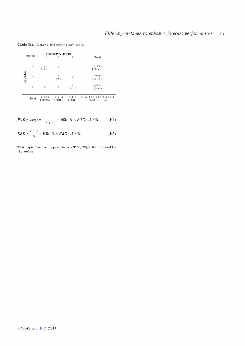
Table B1 is an example of a generic 3×3 contingency ta-ble where the observations and simulations are divided intothree categories delimited by two thresholds. PC, PODi andEBD can be defined using a,b,c,d,e,f,g,h,i (number of timesin which an observation and a simulation fall inside eachcategory) and N (the total events). The percentage of cor-rect detection PC is defined in Eq.B1 where PC = 100% isthe best score; the probability to detect the value of a pa-rameter inside a specific range of values (PODi) is given byEq.B2-Eq.B4 where PODi = 100% is the best score. The ex-tremely bad detection (EBD) probability is given by Eq.B5where EBD = 0% is the best score. For a total random pre-diction and in case of a 3×3 contingency table we have a = b= ... = i = N/9 and PC = PODi = 33% and EBD = 22.2%.

PC =a + e + i

N× 100; 0% ≤ PC ≤ 100% (B1)

POD(event1) =a

a + d + g× 100; 0% ≤ POD ≤ 100% (B2)

POD(event2) =e

b + e + h× 100; 0% ≤ POD ≤ 100% (B3)

MNRAS 000, 1–15 (2019)

Filtering methods to enhance forecast performances 15

Table B1. Generic 3×3 contingency table.

IntervalsOBSERVATIONS

1 2 3 Total

MODEL

1a

b ca+b+c

(hit 1) 1 (Model)

2 de

fd+e+f

(hit 2) 2 (Model)

3 g hi g+h+i

(hit 3) 3 (Model)

Totala+d+g b+e+h c+f+i N=a+b+c+d+e+f+g+h+i1 (OBS) 2 (OBS) 3 (OBS) Total of events

POD(event3) =i

c + f + i× 100; 0% ≤ POD ≤ 100% (B4)

EBD =c + g

N× 100; 0% ≤ EBD ≤ 100% (B5)

This paper has been typeset from a TEX/LATEX file prepared by

the author.

MNRAS 000, 1–15 (2019)