Performance Prediction and Automated Tuning ofRandomized and Parametric Algorithms

Frank Hutter1, Youssef Hamadi2, Holger H. Hoos1, and Kevin Leyton-Brown1

1 University of British Columbia, 2366 Main Mall, Vancouver BC, V6T1Z4, Canada{hutter,kevinlb,hoos}@cs.ubc.ca

2 Microsoft Research, 7 JJ Thomson Ave, Cambridge, UKyoussefh@microsoft.com

Abstract. Machine learning can be utilized to build models that predict the run-time of search algorithms for hard combinatorial problems. Such empirical hard-ness models have previously been studied for complete, deterministic search algo-rithms. In this work, we demonstrate that such models can also make surprisinglyaccurate predictions of the run-time distributions of incomplete and randomizedsearch methods, such as stochastic local search algorithms. We also show for thefirst time how information about an algorithm’s parameter settings can be incor-porated into a model, and how such models can be used to automatically adjustthe algorithm’s parameters on a per-instance basis in order to optimize its perfor-mance. Empirical results for Novelty+ and SAPS on structured and unstructuredSAT instances show very good predictive performance and significant speedupsof our automatically determined parameter settings when compared to the defaultand best fixed distribution-specific parameter settings.

1 Introduction

The last decade has seen a dramatic rise in our ability to solve combinatorial optimiza-tion problems in many practical applications. High-performance heuristic algorithmsincreasingly exploit problem instance structure. Thus, knowledge about the relation-ship between this structure and algorithm behavior forms an important basis for thedevelopment and successful application of such algorithms. This has inspired a largeamount of research on methods for extracting and acting upon such information. Theserange from search space analysis to automated algorithm selection and tuning methods.

An increasing number of studies explore the use of machine learning techniques inthis context [15, 18, 7, 5, 8]. One recent approach uses linear basis function regressionto obtain models of the time an algorithm will require to solve a given problem instance[19, 22]. These so-called empirical hardness models can be used to obtain insights intothe factors responsible for an algorithm’s performance, or to induce distributions ofproblem instances that are challenging for a given algorithm. They can also be leveragedto select among several different algorithms for solving a given problem instance.

In this paper, we extend on this work in three significant ways. First, past workon empirical hardness models has focused exclusively on complete, deterministic algo-rithms. Our first goal is to show that the same approach can be used to predict sufficientstatistics of the run-time distributions (RTDs) of incomplete, randomized algorithms,

and in particular of stochastic local search (SLS) algorithms for SAT. This is impor-tant because SLS algorithms are among the best existing techniques for solving a widerange of hard combinatorial problems, including hard subclasses of SAT [14].

The behavior of many randomized heuristic algorithms is controlled by parameterswith continuous or large discrete domains. This holds in particular for most state-of-the-art SLS algorithms. For example, the performance of WalkSAT algorithms suchas Novelty [20] or Novelty+ [12] depends critically on the setting of a noise parameterwhose optimal value is known to depend on the given SAT instance [13]. Understandingthe relationship between parameter settings and the run-time behavior of an algorithmis of substantial interest for both scientific and pragmatic reasons, as it can exposeweaknesses of a given search algorithm and help to avoid the detrimental impact ofpoor parameter settings. Thus, our second goal is to extend empirical hardness modelsto include algorithm parameters in addition to features of the given problem instance.

Finally, hardness models could also be used to automatically determine good param-eter settings. Thus, an algorithm’s performance could be optimized for each probleminstance without any human intervention or significant overhead. Our final goal is toexplore the potential of such an approach for automatic per-instance parameter tuning.

In what follows, we show that we have achieved all three of our goals by reportingthe results of experiments with SLS algorithms for SAT.3 Specifically, we consideredtwo high-performance SLS algorithms for SAT, Novelty+ [12] and SAPS [17], and sev-eral widely-studied structured and unstructured instance distributions. In section 2, weshow how to build models that predict the sufficient statistics of RTDs for randomizedalgorithms. Empirical results demonstrate that we can predict the median run-time forour test distributions with surprising accuracy (we achieve correlation coefficients be-tween predicted and actual run-time of up to 0.995), and that based on this statistic wecan also predict the complete exponential RTDs Novelty+ and SAPS exhibit. Section 3describes how empirical hardness models can be extended to incorporate algorithm pa-rameters; empirical results still demonstrate excellent performance for this harder task(correlation coefficients reach up to 0.98). Section 4 shows that these models can beleveraged to perform automatic per-instance parameter tuning that results in significantreductions of the algorithm’s run-time compared to using default settings (speedups ofup to two orders of magnitude) or even the best fixed parameter values for the giveninstance distribution (speedups of up to an order of magnitude). Section 5 describeshow Bayesian techniques can be leveraged when predicting run-time for test distribu-tions that differ from the one used for training of the empirical hardness model. Finally,Section 6 concludes the paper and points out future work.

2 Run-time Prediction: Randomized Algorithms

Previous work [19, 22] has shown that it is possible to predict the run-time of deter-ministic tree-search algorithms for combinatorial problems using supervised machine

3 We should note that our approach is not limited to SLS algorithms (it applies as well to e.g.,randomized tree-search methods). Furthermore our techniques are not especially tuned to theSAT domain, though the features we use were created with some domain knowledge. In ex-perimental work it is obviously necessary to choose some specific domain. We have chosen tostudy the SAT problem because it is the prototypical and best-studied NP-complete problemand there exists a great variety of SAT benchmark instances and solvers.

learning techniques. In this section, we demonstrate that similar techniques are able topredict the run-time of algorithms which are both randomized and incomplete. We sup-port our arguments by presenting the results of experiments involving two competitivelocal search algorithms for SAT.

2.1 Prediction of sufficient statistics for run-time distributions

It has been shown in the literature that high-performance randomized local search al-gorithms tend to exhibit exponential run-time distributions [14], meaning that the run-times of two runs that differ only in their random seeds can easily vary by more than oneorder of magnitude. Even more extreme variability in run-time has been observed forrandomized complete search algorithms [10]. Due to this inherent randomness of thealgorithm (and since we do not incorporate information on a particular run), we haveto predict a run-time distribution, that is, a probability distribution over the amountof time an algorithm will take to solve the problem. Run-time distributions for manyrandomized algorithms closely resemble standard parametric distributions, such as theexponential or the Weibull distribution (see, e.g., [14]). These parametric distributionsare completely specified by a small number of sufficient statistics; for example, an ex-ponential distribution is completely specified by its median (or any other quantile) or itsmean. It follows that by predicting these sufficient statistics, a prediction for the entirerun-time distribution for an unseen instance can be obtained.

Note that for randomized algorithms, the error in a model’s predictions can bethought of as consisting of two components, one of which describes the extent to whichthe model fails to describe the data, and the second of which expresses the inherentnoise in the employed summary statistics due to randomness of the algorithm. This lat-ter component reduces as we increase the number of runs from which we extract thestatistic. We demonstrate this later in this section (Figures 1(a) and 1(b)): while em-pirical hardness models of SLS algorithms are able to predict the run-times of singleruns reasonably well, their predictions of median run-times over a larger set of runs aremuch more accurate.

Our approach for run-time prediction of randomized incomplete algorithms largelyfollows the linear regression approach of [19]. We have previously explored othertechniques, namely support vector machine regression, multivariate adaptive regres-sion splines (MARS), and lasso regression, none of which improved our results signifi-cantly.4 While we can handle both complete and incomplete algorithms, we restrict ourexperiments to incomplete local search algorithms. We note, however, that an extensionof our work to randomized tree search algorithms would be straightforward.

In order to predict the run-time of an algorithm A on a distribution D of instances,we draw an i.i.d. sample of N instances fromD. For each instance sn in this training set,A is run some constant number of times and an empirical fit rn of the sufficient statisticsof interest is recorded. Note that rn is a 1×M vector if there are M sufficient statisticsof interest. We also compute a set of 46 instance features xn = [xn,1, . . . , xn,k] foreach instance. This set is a subset of the features used in [22], including basic statistics,

4 Preliminary experiments (see Section 5) suggest that Gaussian processes can increase perfor-mance, especially when the amount of available data is small, but their cubic scaling behaviorin the number of data points complicates their use in practice.

graph-based features, local search probes, and DPLL-based measures.5 We restrictedthe subset of features because some features timed out for large instances – the compu-tation of all our 46 features took just over 2 seconds for each instance.

Given this data for all the training instances, a function f(x) is fitted that, giventhe features xn of an instance, approximates A’s median run-time rn. In linear ba-sis function regression, we construct this function by first generating a set of moreexpressive basis functions φn = φ(xn) = [φ1(xn), . . . , φD(xn)] which can includearbitrarily complex functions of all features xn of an instance sn, or simply the raw fea-tures themselves. These basis functions typically contain a number of elements whichare either unpredictive or highly correlated, so this set should be reduced by apply-ing some form of feature selection. We then use ridge regression to fit the D × Mmatrix of free parameters w of a linear function fw(xn) = φ(xn)T w, that is, wecompute w = (δI + ΦT Φ)−1ΦT r, where δ is a small regularization constant (setto 10−2 in our experiments), Φ is the N × D design matrix Φ = [φT

1 , . . . , φTN ]T ,

and r = [r1T , . . . , rN

T ]T . Given a new, unseen instance sN+1, a prediction of the Msufficient statistics can be obtained by computing the instance features xN+1 and eval-uating fw(xN+1) = φ(xN+1)T w. One advantage of the simplicity of ridge regressionis a low computational complexity of Θ(max{D3, D2N, DNM}) for training and ofΘ(DM) for prediction for an unseen test instance.

2.2 Experimental setup and empirical results for predicting median run-time

We performed experiments for the prediction of median run-time using two SLS algo-rithms, SAPS and Novelty+. In this section we fix SAPS parameters to their defaults〈α, ρ, Psmooth〉 = 〈1.3, 0.8, 0.05〉. For Novelty+, we use its default parameter setting〈noise, wp〉 = 〈50, 0.01〉 for unstructured instances; for structured instances whereNovelty+ is known to perform better with lower noise settings, we chose 〈noise, wp〉 =〈10, 0.01〉 (with noise=50% the majority of runs did not finish within an hour of CPUtime). We consider models that incorporate multiple parameter settings in the next sec-tion. Since, based on previous studies of these algorithms, we expect approximately ex-ponential run-time distributions, the empirical fit of the sufficient statistics rn for eachtraining instance sn simply consists of recording the median of a fixed number of runs.

In our experiments, we used six widely-studied SAT benchmark distributions, threeof which consist of unstructured instances and the other three of structured instances.The first two distributions we studied each consisted of 20,000 uniform-random 3-SATinstances with 400 variables; the first (CV-var) varied the clauses-to-variables ratiobetween 3.26 and 5.26, while the second (CV-fixed) fixed c/v = 4.26. These distri-butions were previously studied in [22], facilitating a comparison of our results withpast work. Our third unstructured distribution (SAT04) consisted of 3,000 random un-structured instances generated with the two generators used for the 2004 SAT solvercompetition (with identical parameters) and was employed to evaluate our automatedparameter tuning procedure on a competition benchmark.

Our first two structured distributions are different variants of quasigroup comple-tion problems. The first one (QCP) consisted of 30,000 hard quasigroup completion

5 Information on precisely which features we used, as well as the restof our experimental data and Matlab code, is available online athttp://www.cs.ubc.ca/labs/beta/Projects/RandomHardness/.

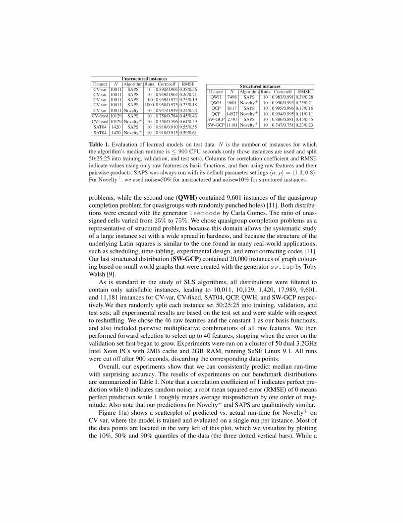
Unstructured instancesDataset N Algorithm Runs Corrcoeff RMSECV-var 10011 SAPS 1 0.892/0.906 0.38/0.36CV-var 10011 SAPS 10 0.949/0.964 0.26/0.21CV-var 10011 SAPS 100 0.959/0.972 0.23/0.19CV-var 10011 SAPS 1000 0.958/0.975 0.23/0.18CV-var 10011 Novelty+ 10 0.947/0.949 0.24/0.23

CV-fixed 10129 SAPS 10 0.758/0.784 0.45/0.43CV-fixed 10129 Novelty+ 10 0.558/0.596 0.61/0.59SAT04 1420 SAPS 10 0.918/0.910 0.55/0.55SAT04 1420 Novelty+ 10 0.918/0.915 0.59/0.61

Structured instancesDataset N Algorithm Runs Corrcoeff RMSEQWH 7498 SAPS 10 0.983/0.991 0.38/0.28QWH 9601 Novelty+ 10 0.990/0.993 0.25/0.21QCP 8117 SAPS 10 0.995/0.996 0.17/0.16QCP 14927 Novelty+ 10 0.994/0.995 0.11/0.11

SW-GCP 2740 SAPS 10 0.886/0.881 0.45/0.45SW-GCP 11181 Novelty+ 10 0.747/0.751 0.23/0.23

Table 1. Evaluation of learned models on test data. N is the number of instances for whichthe algorithm’s median runtime is ≤ 900 CPU seconds (only those instances are used and split50:25:25 into training, validation, and test sets). Columns for correlation coefficient and RMSEindicate values using only raw features as basis functions, and then using raw features and theirpairwise products. SAPS was always run with its default parameter settings 〈α, ρ〉 = 〈1.3, 0.8〉.For Novelty+, we used noise=50% for unstructured and noise=10% for structured instances.

problems, while the second one (QWH) contained 9,601 instances of the quasigroupcompletion problem for quasigroups with randomly punched holes) [11]. Both distribu-tions were created with the generator lsencode by Carla Gomes. The ratio of unas-signed cells varied from 25% to 75%. We chose quasigroup completion problems as arepresentative of structured problems because this domain allows the systematic studyof a large instance set with a wide spread in hardness, and because the structure of theunderlying Latin squares is similar to the one found in many real-world applications,such as scheduling, time-tabling, experimental design, and error correcting codes [11].Our last structured distribution (SW-GCP) contained 20,000 instances of graph colour-ing based on small world graphs that were created with the generator sw.lsp by TobyWalsh [9].

As is standard in the study of SLS algorithms, all distributions were filtered tocontain only satisfiable instances, leading to 10,011, 10,129, 1,420, 17,989, 9,601,and 11,181 instances for CV-var, CV-fixed, SAT04, QCP, QWH, and SW-GCP respec-tively.We then randomly split each instance set 50:25:25 into training, validation, andtest sets; all experimental results are based on the test set and were stable with respectto reshuffling. We chose the 46 raw features and the constant 1 as our basis functions,and also included pairwise multiplicative combinations of all raw features. We thenperformed forward selection to select up to 40 features, stopping when the error on thevalidation set first began to grow. Experiments were run on a cluster of 50 dual 3.2GHzIntel Xeon PCs with 2MB cache and 2GB RAM, running SuSE Linux 9.1. All runswere cut off after 900 seconds, discarding the corresponding data points.

Overall, our experiments show that we can consistently predict median run-timewith surprising accuracy. The results of experiments on our benchmark distributionsare summarized in Table 1. Note that a correlation coefficient of 1 indicates perfect pre-diction while 0 indicates random noise; a root mean squared error (RMSE) of 0 meansperfect prediction while 1 roughly means average misprediction by one order of mag-nitude. Also note that our predictions for Novelty+ and SAPS are qualitatively similar.

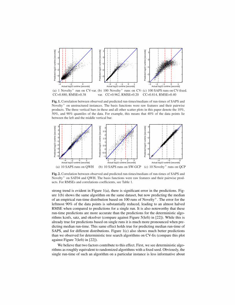
Figure 1(a) shows a scatterplot of predicted vs. actual run-time for Novelty+ onCV-var, where the model is trained and evaluated on a single run per instance. Most ofthe data points are located in the very left of this plot, which we visualize by plottingthe 10%, 50% and 90% quantiles of the data (the three dotted vertical bars). While a

−4 −2 0−4

−3

−2

−1

0

1

Actual log10 runtime [seconds]

Pre

dict

ed lo

g10

runt

ime

[sec

onds

]

(a) 1 Novelty+ run on CV-var.CC=0.880, RMSE=0.38

−3 −2 −1 0 1

−3

−2

−1

0

1

Actual log10 runtime [seconds]

Pre

dict

ed lo

g10

runt

ime

[sec

onds

]

(b) 100 Novelty+ runs on CV-var. CC=0.962, RMSE=0.20

−3 −2 −1 0 1−3

−2

−1

0

1

Actual log10 runtime [seconds]

Pre

dict

ed lo

g10

runt

ime

[sec

onds

]

(c) 100 SAPS runs on CV-fixed.CC=0.814, RMSE=0.40

Fig. 1. Correlation between observed and predicted run-times/medians of run-times of SAPS andNovelty+ on unstructured instances. The basis functions were raw features and their pairwiseproducts. The three vertical bars in these and all other scatter plots in this paper denote the 10%,50%, and 90% quantiles of the data. For example, this means that 40% of the data points liebetween the left and the middle vertical bar.

−4 −2 0 2

−5

−4

−3

−2

−1

0

1

2

3

Actual log10 runtime [seconds]

Pre

dict

ed lo

g10

runt

ime

[sec

onds

]

(a) 10 SAPS runs on QWH

−1 0 1 2 3

−1

−0.5

0

0.5

1

1.5

2

2.5

3

Actual log10 runtime [seconds]

Pre

dict

ed lo

g10

runt

ime

[sec

onds

]

(b) 10 SAPS runs on SW-GCP

−4 −2 0

−5

−4

−3

−2

−1

0

Actual log10 runtime [seconds]

Pre

dict

ed lo

g10

runt

ime

[sec

onds

]

(c) 10 Novelty+ runs on QCP

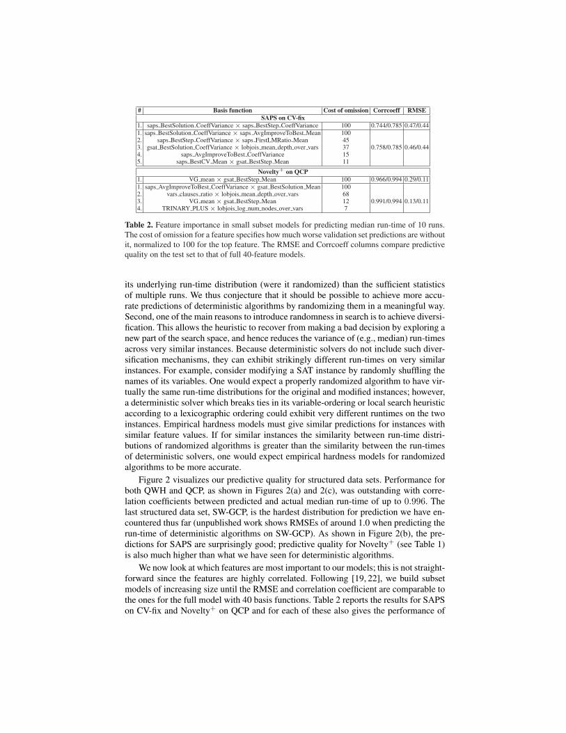
Fig. 2. Correlation between observed and predicted run-times/medians of run-times of SAPS andNovelty+ on SAT04 and QWH. The basis functions were raw features and their pairwise prod-ucts. For RMSEs and correlations coefficients, see Table 1.

strong trend is evident in Figure 1(a), there is significant error in the predictions. Fig-ure 1(b) shows the same algorithm on the same dataset, but now predicting the medianof an empirical run-time distribution based on 100 runs of Novelty+. The error for theleftmost 90% of the data points is substantially reduced, leading to an almost halvedRMSE when compared to predictions for a single run. It is also noteworthy that theserun-time predictions are more accurate than the predictions for the deterministic algo-rithms kcnfs, satz, and oksolver (compare against Figure 5(left) in [22]). While this isalready true for predictions based on single runs it is much more pronounced when pre-dicting median run-time. This same effect holds true for predicting median run-time ofSAPS, and for different distributions. Figure 1(c) also shows much better predictionsthan we observed for deterministic tree search algorithms on CV-fix (compare this plotagainst Figure 7(left) in [22]).

We believe that two factors contribute to this effect. First, we see deterministic algo-rithms as roughly equivalent to randomized algorithms with a fixed seed. Obviously, thesingle run-time of such an algorithm on a particular instance is less informative about

# Basis function Cost of omission Corrcoeff RMSESAPS on CV-fix

1. saps BestSolution CoeffVariance× saps BestStep CoeffVariance 100 0.744/0.785 0.47/0.441. saps BestSolution CoeffVariance× saps AvgImproveToBest Mean 1002. saps BestStep CoeffVariance× saps FirstLMRatio Mean 453. gsat BestSolution CoeffVariance× lobjois mean depth over vars 37 0.758/0.785 0.46/0.444. saps AvgImproveToBest CoeffVariance 155. saps BestCV Mean× gsat BestStep Mean 11

Novelty+ on QCP1. VG mean× gsat BestStep Mean 100 0.966/0.994 0.29/0.111. saps AvgImproveToBest CoeffVariance× gsat BestSolution Mean 1002. vars clauses ratio× lobjois mean depth over vars 683. VG mean× gsat BestStep Mean 12 0.991/0.994 0.13/0.114. TRINARY PLUS× lobjois log num nodes over vars 7

Table 2. Feature importance in small subset models for predicting median run-time of 10 runs.The cost of omission for a feature specifies how much worse validation set predictions are withoutit, normalized to 100 for the top feature. The RMSE and Corrcoeff columns compare predictivequality on the test set to that of full 40-feature models.

its underlying run-time distribution (were it randomized) than the sufficient statisticsof multiple runs. We thus conjecture that it should be possible to achieve more accu-rate predictions of deterministic algorithms by randomizing them in a meaningful way.Second, one of the main reasons to introduce randomness in search is to achieve diversi-fication. This allows the heuristic to recover from making a bad decision by exploring anew part of the search space, and hence reduces the variance of (e.g., median) run-timesacross very similar instances. Because deterministic solvers do not include such diver-sification mechanisms, they can exhibit strikingly different run-times on very similarinstances. For example, consider modifying a SAT instance by randomly shuffling thenames of its variables. One would expect a properly randomized algorithm to have vir-tually the same run-time distributions for the original and modified instances; however,a deterministic solver which breaks ties in its variable-ordering or local search heuristicaccording to a lexicographic ordering could exhibit very different runtimes on the twoinstances. Empirical hardness models must give similar predictions for instances withsimilar feature values. If for similar instances the similarity between run-time distri-butions of randomized algorithms is greater than the similarity between the run-timesof deterministic solvers, one would expect empirical hardness models for randomizedalgorithms to be more accurate.

Figure 2 visualizes our predictive quality for structured data sets. Performance forboth QWH and QCP, as shown in Figures 2(a) and 2(c), was outstanding with corre-lation coefficients between predicted and actual median run-time of up to 0.996. Thelast structured data set, SW-GCP, is the hardest distribution for prediction we have en-countered thus far (unpublished work shows RMSEs of around 1.0 when predicting therun-time of deterministic algorithms on SW-GCP). As shown in Figure 2(b), the pre-dictions for SAPS are surprisingly good; predictive quality for Novelty+ (see Table 1)is also much higher than what we have seen for deterministic algorithms.

We now look at which features are most important to our models; this is not straight-forward since the features are highly correlated. Following [19, 22], we build subsetmodels of increasing size until the RMSE and correlation coefficient are comparable tothe ones for the full model with 40 basis functions. Table 2 reports the results for SAPSon CV-fix and Novelty+ on QCP and for each of these also gives the performance of

−4 −2 0 2

−5

−4

−3

−2

−1

0

1

2

3

Actual log10 runtime [seconds]

Pre

dict

ed lo

g10

runt

ime

[sec

onds

]

(a) Predictions of median run-time, instances q0.25 and q0.75

10−4

10−2

0

0.2

0.4

0.6

0.8

1

Runtime [seconds]

Pro

ba

bili

ty o

f su

cce

ss

True empirical RTDPredicted RTD

(b) Easy QCP instance (q0.25)

10−4

10−2

100

0

0.2

0.4

0.6

0.8

1

Runtime [seconds]

Pro

ba

bili

ty o

f su

cce

ss

True empirical RTDPredicted RTD

(c) Hard QCP instance (q0.75)

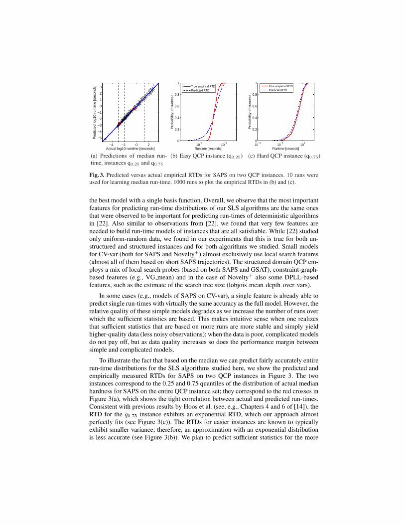
Fig. 3. Predicted versus actual empirical RTDs for SAPS on two QCP instances. 10 runs wereused for learning median run-time, 1000 runs to plot the empirical RTDs in (b) and (c).

the best model with a single basis function. Overall, we observe that the most importantfeatures for predicting run-time distributions of our SLS algorithms are the same onesthat were observed to be important for predicting run-times of deterministic algorithmsin [22]. Also similar to observations from [22], we found that very few features areneeded to build run-time models of instances that are all satisfiable. While [22] studiedonly uniform-random data, we found in our experiments that this is true for both un-structured and structured instances and for both algorithms we studied. Small modelsfor CV-var (both for SAPS and Novelty+) almost exclusively use local search features(almost all of them based on short SAPS trajectories). The structured domain QCP em-ploys a mix of local search probes (based on both SAPS and GSAT), constraint-graph-based features (e.g., VG mean) and in the case of Novelty+ also some DPLL-basedfeatures, such as the estimate of the search tree size (lobjois mean depth over vars).

In some cases (e.g., models of SAPS on CV-var), a single feature is already able topredict single run-times with virtually the same accuracy as the full model. However, therelative quality of these simple models degrades as we increase the number of runs overwhich the sufficient statistics are based. This makes intuitive sense when one realizesthat sufficient statistics that are based on more runs are more stable and simply yieldhigher-quality data (less noisy observations); when the data is poor, complicated modelsdo not pay off, but as data quality increases so does the performance margin betweensimple and complicated models.

To illustrate the fact that based on the median we can predict fairly accurately entirerun-time distributions for the SLS algorithms studied here, we show the predicted andempirically measured RTDs for SAPS on two QCP instances in Figure 3. The twoinstances correspond to the 0.25 and 0.75 quantiles of the distribution of actual medianhardness for SAPS on the entire QCP instance set; they correspond to the red crosses inFigure 3(a), which shows the tight correlation between actual and predicted run-times.Consistent with previous results by Hoos et al. (see, e.g., Chapters 4 and 6 of [14]), theRTD for the q0.75 instance exhibits an exponential RTD, which our approach almostperfectly fits (see Figure 3(c)). The RTDs for easier instances are known to typicallyexhibit smaller variance; therefore, an approximation with an exponential distributionis less accurate (see Figure 3(b)). We plan to predict sufficient statistics for the more

general distributions needed to characterise such RTDs, such as Weibull and generalisedexponential distributions, in the future.

3 Run-time Prediction: Parametric Algorithms

It is well known that the behavior of most high-performance SLS algorithms is con-trolled by one or more parameters, and that these parameters often have a substantialeffect on the algorithm’s performance [14]. In the previous section, we showed thatgood empirical hardness models can be constructed when these parameters are heldconstant. In practice, however, we want to be able to change these parameter valuesand to understand what will happen when we do. In this section, we demonstrate thatit is possible to incorporate parameters into empirical hardness models for randomized,incomplete algorithms. Our techniques should carry over directly to both determinis-tic and complete parametric algorithms (in the case of deterministic algorithms usingsingle run-times instead of sufficient statistics of RTDs).

Our approach is to learn a function g(x, c) that takes as inputs both the features xn

of an instance sn and the parameter configuration c of an algorithmA, and that approx-imates sufficient statistics of A’s RTD when run on instance sn with parameter config-uration c. In the training phase, for each training instance sn we run A some constantnumber of times with a set of parameter configurations cn = {cn,1, . . . , cn,kn}, andcollect fits of the sufficient statistics rn = [rT

n,1, . . . , rTn,kn

]T of the corresponding em-pirical run-time distributions. We also compute sn’s features xn. The key change fromthe approach in Section 2.1 is that now the parameters that were used to generate an〈instance,run-time〉 pair are effectively treated as additional features of that training ex-ample. We define a new set of basis functions φ(xn, cn,j) = [φ1(xn, cn,j), . . . , φD(xn, cn,j)]whose domain now consists of the cross product of features and parameter configura-tions. For each instance sn and parameter configuration cn,j , we will have a row inthe design matrix Φ that contains φ(xn, cn,j)T — that is, the design matrix now con-tains nk rows for every training instance. The target vector r = [rT

1 , . . . , rTN ]T just

stacks all the sufficient statistics on top of each other. We learn the function gw(x, c) =φ(x, c)T w by applying ridge regression as in Section 2.1.

Our experiments in this section concentrate on predicting median run-time of SAPSsince it has three interdependent, continuous parameters, as compared to Novelty+

which has only two parameters, one of which (wp) is typically set to a default valuethat results in uniformly good performance. This difference notwithstanding, we ob-served qualitatively similar results with Novelty+. Note that the approach outlinedabove allows one to use different parameter settings for each training instance. Howto pick these parameter settings for training in the most informative way is an inter-esting experimental design which invites application of active learning techniques; weplan to tackle it in future work. In this study, for SAPS we used all combinations ofα ∈ {1.2, 1.3, 1.4} and ρ ∈ {0, .1, .2, .3, .4, .5, .6, .7, .8, .9}, keeping Psmooth = 0.05constant since its effect is highly correlated with that of ρ. For Novelty+, we usednoise ∈ {10, 20, 30, 40, 50, 60}, fixing wp = 0.01.

As basis functions, we used multiplicative combinations of the raw instance featuresxn and a 2nd order expansion of all non-fixed (continuous) parameter settings. For Kraw features (K = 46 in our experiments), this meant 3K basis functions for Novelty+,

−4 −2 0 2

−4

−2

0

2

Actual log10 runtime [seconds]

Pre

dict

ed lo

g10

runt

ime

[sec

onds

]

(a) SAPS on QWH, 30 set-tings

−2 0 2−3

−2

−1

0

1

2

3

Actual log10 runtime [seconds]

Pre

dict

ed lo

g10

runt

ime

[sec

onds

]

(b) 5 symbol-coded in-stances

0 .2 .4 .6 .8 0 .2 .4 .6 .8 0 .2 .4 .6 .8−1.5

−1

−0.5

0

0.5

1

1.5

rho

Lo

g1

0 m

ed

ian

ru

ntim

e [

seco

nd

s]

true SAPS median

prediction,alpha = 1.2

prediction,alpha = 1.3

prediction,alpha = 1.4

(c) Run-time predictions for median-hard instance

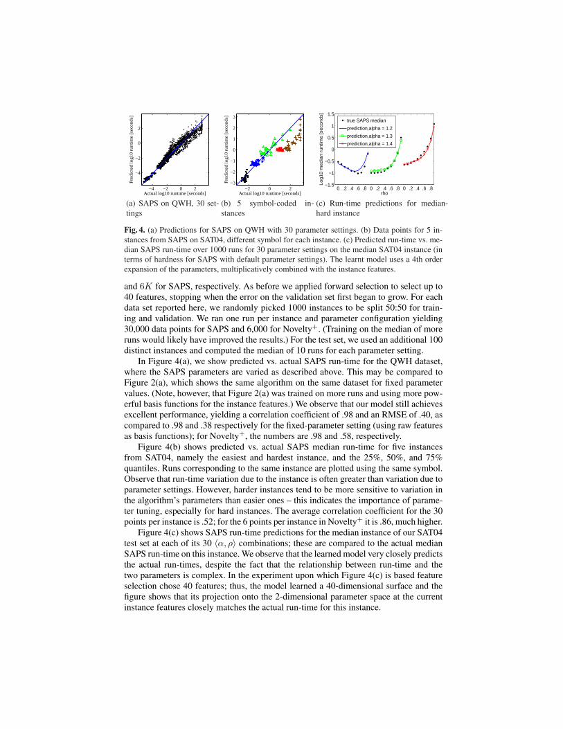
Fig. 4. (a) Predictions for SAPS on QWH with 30 parameter settings. (b) Data points for 5 in-stances from SAPS on SAT04, different symbol for each instance. (c) Predicted run-time vs. me-dian SAPS run-time over 1000 runs for 30 parameter settings on the median SAT04 instance (interms of hardness for SAPS with default parameter settings). The learnt model uses a 4th orderexpansion of the parameters, multiplicatively combined with the instance features.

and 6K for SAPS, respectively. As before we applied forward selection to select up to40 features, stopping when the error on the validation set first began to grow. For eachdata set reported here, we randomly picked 1000 instances to be split 50:50 for train-ing and validation. We ran one run per instance and parameter configuration yielding30,000 data points for SAPS and 6,000 for Novelty+. (Training on the median of moreruns would likely have improved the results.) For the test set, we used an additional 100distinct instances and computed the median of 10 runs for each parameter setting.

In Figure 4(a), we show predicted vs. actual SAPS run-time for the QWH dataset,where the SAPS parameters are varied as described above. This may be compared toFigure 2(a), which shows the same algorithm on the same dataset for fixed parametervalues. (Note, however, that Figure 2(a) was trained on more runs and using more pow-erful basis functions for the instance features.) We observe that our model still achievesexcellent performance, yielding a correlation coefficient of .98 and an RMSE of .40, ascompared to .98 and .38 respectively for the fixed-parameter setting (using raw featuresas basis functions); for Novelty+, the numbers are .98 and .58, respectively.

Figure 4(b) shows predicted vs. actual SAPS median run-time for five instancesfrom SAT04, namely the easiest and hardest instance, and the 25%, 50%, and 75%quantiles. Runs corresponding to the same instance are plotted using the same symbol.Observe that run-time variation due to the instance is often greater than variation due toparameter settings. However, harder instances tend to be more sensitive to variation inthe algorithm’s parameters than easier ones – this indicates the importance of parame-ter tuning, especially for hard instances. The average correlation coefficient for the 30points per instance is .52; for the 6 points per instance in Novelty+ it is .86, much higher.

Figure 4(c) shows SAPS run-time predictions for the median instance of our SAT04test set at each of its 30 〈α, ρ〉 combinations; these are compared to the actual medianSAPS run-time on this instance. We observe that the learned model very closely predictsthe actual run-times, despite the fact that the relationship between run-time and thetwo parameters is complex. In the experiment upon which Figure 4(c) is based featureselection chose 40 features; thus, the model learned a 40-dimensional surface and thefigure shows that its projection onto the 2-dimensional parameter space at the currentinstance features closely matches the actual run-time for this instance.

Set Algo Gross corr RMSE Corr per inst. best fixed params sbpi swpi sdef sfixed

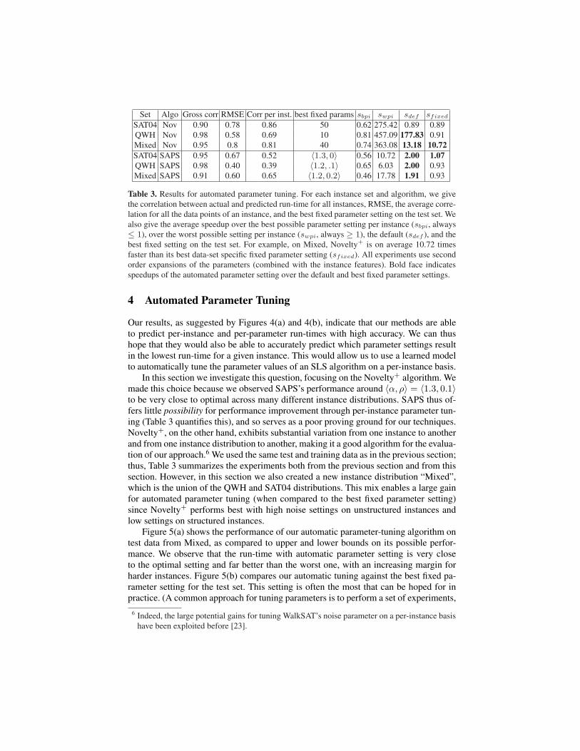
SAT04 Nov 0.90 0.78 0.86 50 0.62 275.42 0.89 0.89QWH Nov 0.98 0.58 0.69 10 0.81 457.09 177.83 0.91Mixed Nov 0.95 0.8 0.81 40 0.74 363.08 13.18 10.72SAT04 SAPS 0.95 0.67 0.52 〈1.3, 0〉 0.56 10.72 2.00 1.07QWH SAPS 0.98 0.40 0.39 〈1.2, .1〉 0.65 6.03 2.00 0.93Mixed SAPS 0.91 0.60 0.65 〈1.2, 0.2〉 0.46 17.78 1.91 0.93

Table 3. Results for automated parameter tuning. For each instance set and algorithm, we givethe correlation between actual and predicted run-time for all instances, RMSE, the average corre-lation for all the data points of an instance, and the best fixed parameter setting on the test set. Wealso give the average speedup over the best possible parameter setting per instance (sbpi, always≤ 1), over the worst possible setting per instance (swpi, always ≥ 1), the default (sdef ), and thebest fixed setting on the test set. For example, on Mixed, Novelty+ is on average 10.72 timesfaster than its best data-set specific fixed parameter setting (sfixed). All experiments use secondorder expansions of the parameters (combined with the instance features). Bold face indicatesspeedups of the automated parameter setting over the default and best fixed parameter settings.

4 Automated Parameter Tuning

Our results, as suggested by Figures 4(a) and 4(b), indicate that our methods are ableto predict per-instance and per-parameter run-times with high accuracy. We can thushope that they would also be able to accurately predict which parameter settings resultin the lowest run-time for a given instance. This would allow us to use a learned modelto automatically tune the parameter values of an SLS algorithm on a per-instance basis.

In this section we investigate this question, focusing on the Novelty+ algorithm. Wemade this choice because we observed SAPS’s performance around 〈α, ρ〉 = 〈1.3, 0.1〉to be very close to optimal across many different instance distributions. SAPS thus of-fers little possibility for performance improvement through per-instance parameter tun-ing (Table 3 quantifies this), and so serves as a poor proving ground for our techniques.Novelty+, on the other hand, exhibits substantial variation from one instance to anotherand from one instance distribution to another, making it a good algorithm for the evalua-tion of our approach.6 We used the same test and training data as in the previous section;thus, Table 3 summarizes the experiments both from the previous section and from thissection. However, in this section we also created a new instance distribution “Mixed”,which is the union of the QWH and SAT04 distributions. This mix enables a large gainfor automated parameter tuning (when compared to the best fixed parameter setting)since Novelty+ performs best with high noise settings on unstructured instances andlow settings on structured instances.

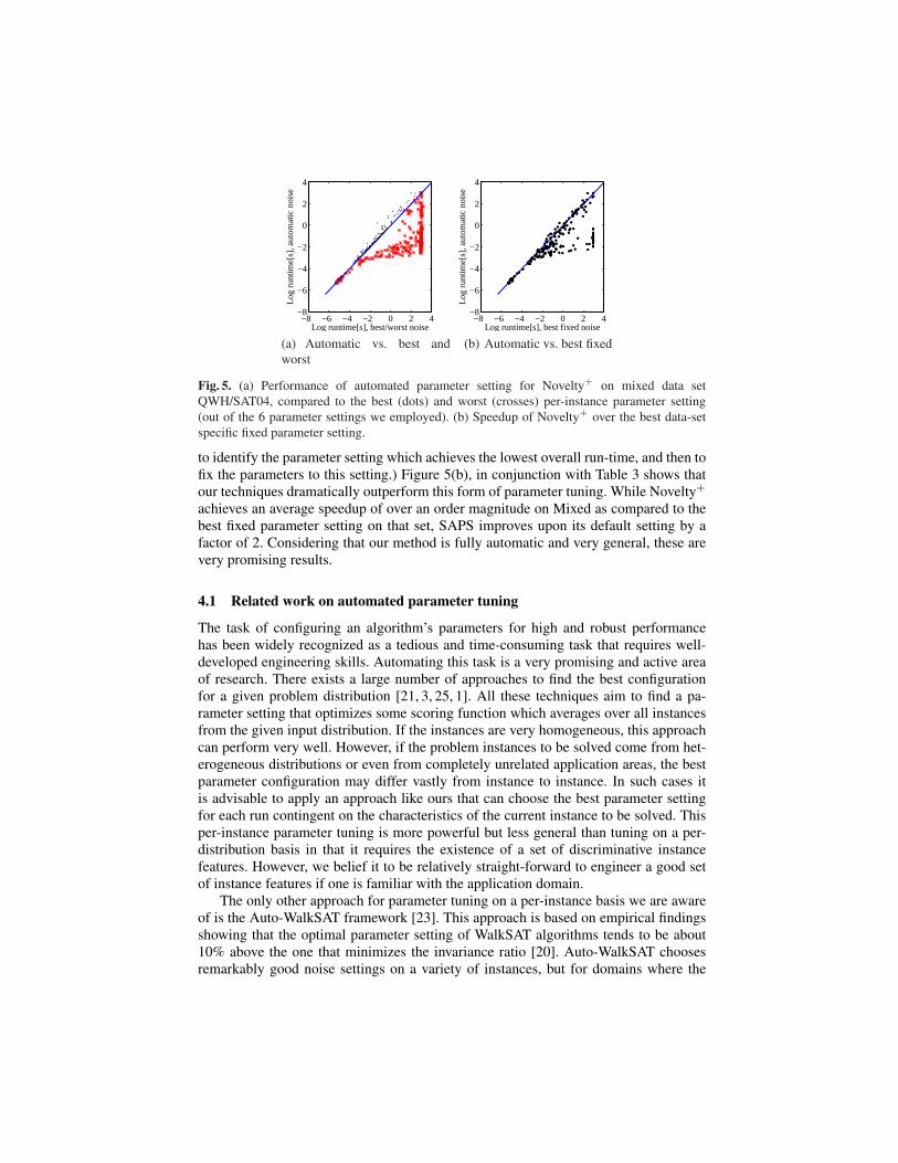
Figure 5(a) shows the performance of our automatic parameter-tuning algorithm ontest data from Mixed, as compared to upper and lower bounds on its possible perfor-mance. We observe that the run-time with automatic parameter setting is very closeto the optimal setting and far better than the worst one, with an increasing margin forharder instances. Figure 5(b) compares our automatic tuning against the best fixed pa-rameter setting for the test set. This setting is often the most that can be hoped for inpractice. (A common approach for tuning parameters is to perform a set of experiments,

6 Indeed, the large potential gains for tuning WalkSAT’s noise parameter on a per-instance basishave been exploited before [23].

−8 −6 −4 −2 0 2 4−8

−6

−4

−2

0

2

4

Log runtime[s], best/worst noise

Log

runt

ime[

s], a

utom

atic

noi

se

(a) Automatic vs. best andworst

−8 −6 −4 −2 0 2 4−8

−6

−4

−2

0

2

4

Log runtime[s], best fixed noise

Log

runt

ime[

s], a

utom

atic

noi

se

(b) Automatic vs. best fixed

Fig. 5. (a) Performance of automated parameter setting for Novelty+ on mixed data setQWH/SAT04, compared to the best (dots) and worst (crosses) per-instance parameter setting(out of the 6 parameter settings we employed). (b) Speedup of Novelty+ over the best data-setspecific fixed parameter setting.

to identify the parameter setting which achieves the lowest overall run-time, and then tofix the parameters to this setting.) Figure 5(b), in conjunction with Table 3 shows thatour techniques dramatically outperform this form of parameter tuning. While Novelty+

achieves an average speedup of over an order magnitude on Mixed as compared to thebest fixed parameter setting on that set, SAPS improves upon its default setting by afactor of 2. Considering that our method is fully automatic and very general, these arevery promising results.

4.1 Related work on automated parameter tuning

The task of configuring an algorithm’s parameters for high and robust performancehas been widely recognized as a tedious and time-consuming task that requires well-developed engineering skills. Automating this task is a very promising and active areaof research. There exists a large number of approaches to find the best configurationfor a given problem distribution [21, 3, 25, 1]. All these techniques aim to find a pa-rameter setting that optimizes some scoring function which averages over all instancesfrom the given input distribution. If the instances are very homogeneous, this approachcan perform very well. However, if the problem instances to be solved come from het-erogeneous distributions or even from completely unrelated application areas, the bestparameter configuration may differ vastly from instance to instance. In such cases itis advisable to apply an approach like ours that can choose the best parameter settingfor each run contingent on the characteristics of the current instance to be solved. Thisper-instance parameter tuning is more powerful but less general than tuning on a per-distribution basis in that it requires the existence of a set of discriminative instancefeatures. However, we belief it to be relatively straight-forward to engineer a good setof instance features if one is familiar with the application domain.

The only other approach for parameter tuning on a per-instance basis we are awareof is the Auto-WalkSAT framework [23]. This approach is based on empirical findingsshowing that the optimal parameter setting of WalkSAT algorithms tends to be about10% above the one that minimizes the invariance ratio [20]. Auto-WalkSAT choosesremarkably good noise settings on a variety of instances, but for domains where the

−6 −4 −2 0 2−6

−5

−4

−3

−2

−1

0

1

2

Actual log10 runtime [seconds]

Pred

icted

log1

0 ru

ntim

e [se

cond

s]

(a) Bayesian linear regression

−6 −4 −2 0 2−6

−5

−4

−3

−2

−1

0

1

2

Actual log10 runtime [seconds]

Pred

icted

log1

0 ru

ntim

e [se

cond

s]

(b) Gaussian process with squared exponen-tial kernel

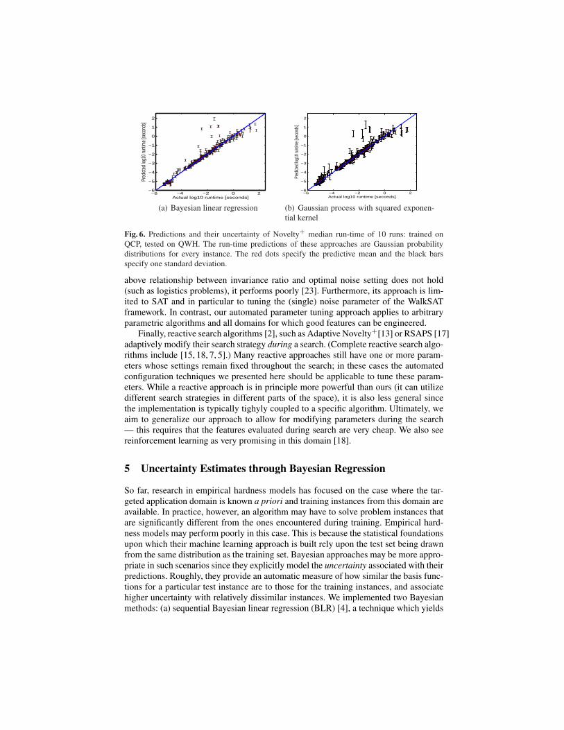
Fig. 6. Predictions and their uncertainty of Novelty+ median run-time of 10 runs: trained onQCP, tested on QWH. The run-time predictions of these approaches are Gaussian probabilitydistributions for every instance. The red dots specify the predictive mean and the black barsspecify one standard deviation.

above relationship between invariance ratio and optimal noise setting does not hold(such as logistics problems), it performs poorly [23]. Furthermore, its approach is lim-ited to SAT and in particular to tuning the (single) noise parameter of the WalkSATframework. In contrast, our automated parameter tuning approach applies to arbitraryparametric algorithms and all domains for which good features can be engineered.

Finally, reactive search algorithms [2], such as Adaptive Novelty+[13] or RSAPS [17]adaptively modify their search strategy during a search. (Complete reactive search algo-rithms include [15, 18, 7, 5].) Many reactive approaches still have one or more param-eters whose settings remain fixed throughout the search; in these cases the automatedconfiguration techniques we presented here should be applicable to tune these param-eters. While a reactive approach is in principle more powerful than ours (it can utilizedifferent search strategies in different parts of the space), it is also less general sincethe implementation is typically tighyly coupled to a specific algorithm. Ultimately, weaim to generalize our approach to allow for modifying parameters during the search— this requires that the features evaluated during search are very cheap. We also seereinforcement learning as very promising in this domain [18].

5 Uncertainty Estimates through Bayesian Regression

So far, research in empirical hardness models has focused on the case where the tar-geted application domain is known a priori and training instances from this domain areavailable. In practice, however, an algorithm may have to solve problem instances thatare significantly different from the ones encountered during training. Empirical hard-ness models may perform poorly in this case. This is because the statistical foundationsupon which their machine learning approach is built rely upon the test set being drawnfrom the same distribution as the training set. Bayesian approaches may be more appro-priate in such scenarios since they explicitly model the uncertainty associated with theirpredictions. Roughly, they provide an automatic measure of how similar the basis func-tions for a particular test instance are to those for the training instances, and associatehigher uncertainty with relatively dissimilar instances. We implemented two Bayesianmethods: (a) sequential Bayesian linear regression (BLR) [4], a technique which yields

mean predictions equivalent to ridge regression but also offers estimates of uncertainty;and (b) Gaussian Process Regression (GPR) [24] with a squared exponential kernel. Wedetail BLR and the potential applications of a Bayesian approach to run-time predictionin an accompanying technical report [16]. Since GPR scales cubically in the number ofdata points, we trained it on a subset of 1000 data points (but used all 9601 data pointsfor BLR). Even so, GPR took roughly 1000 times longer to train.

We evaluated both our methods on two different problems. The first problem is totrain and validate on our QCP data-set and test on our QWH data-set. While these dis-tributions are not identical, our intuition was that they share enough structure to allowmodels trained on one to make good predictions on the other. The second problem wasmuch harder: we trained on data-set SAT04 and tested on a very diverse test set con-taining instances from ten qualitatively different distributions from SATLIB. Figure 6shows predictions and their uncertainty (± one stddev) for both methods on the firstproblem. The two distributions are similar enough to yield very good predictions forboth approaches. While BLR was overconfident on this data set, the uncertainty es-timates of GPR make more sense: they are very small for accurately predicted datapoints and large for mispredicted ones. Both models achieved similar predictive accu-racy (CC/RMSE .97/.45 for BLR; .97/.43 for GPR). For the second problem (spaceconsiderations disallow a figure), BLR showed massive mispredictions (several tens oforders of magnitude) but associated very high uncertainty with the mispredicted in-stances, reflecting their dissimilarity with the training set. GPR showed more reason-able predictions, and also did a good job in claiming high uncertainty about instances forwhich predictive quality was low. Based on these preliminary results, we view Gaussianprocess regression as particularly promising and plan to study its application to run-timeprediction in more detail. However, we note that its scaling behavior somewhat limitsits applications.

6 Conclusion and Future Work

In this work, we have demonstrated that empirical hardness models obtained from linearbasis function regression can be extended to make surprisingly accurate predictions ofthe run-time of randomized, incomplete algorithms, such as Novelty+ and SAPS. Basedon a prediction of sufficient statistics for run-time distributions (RTDs), we showed verygood predictions of the entire empirical RTDs for unseen test instances. We have alsodemonstrated for the first time that empirical hardness models can model the effect ofalgorithm parameter settings on run-time, and that these models can be used as a basisfor automated per-instance parameter tuning. In our experiments, this tuning never hurtand sometimes resulted in substantial and completely automatic performance improve-ments, as compared to default or optimized fixed parameter settings.

There are several natural ways in which this work can be extended. First, we arecurrently studying Bayesian methods for run-time prediction in more detail. We furtherplan to study the extent to which our results generalize to problems other than SAT andin particular, to optimization problems. Finally, we would like to apply active learningapproaches [6] in order to probe the parameter space in the most informative way inorder to reduce training time.

References1. B. Adenso-Daz and M. Laguna. Fine-tuning of algorithms using fractional experimental

design and local search. Operations Research, 54(1), 2006. To appear.2. R. Battiti and M. Brunato. Reactive search: machine learning for memory-based heuristics.

Technical Report DIT-05-058, Universita Degli Studi Di Trento, Dept. of information andcommunication technology, Trento, Italy, September 2005.

3. M. Birattari, T. Stutzle, L. Paquete, and K. Varrentrapp. A racing algorithm for configuringmetaheuristics. In Proc. of GECCO-02, pages 11–18, 2002.

4. C. M. Bishop. Neural Networks for Pattern Recognition. Oxford Univ. Press, 1995.5. T. Carchrae and J. C. Beck. Applying machine learning to low-knowledge control of opti-

mization algorithms. Computational Intelligence, 21(4):372–387, 2005.6. D. A. Cohn, Z. Ghahramani, and M. I. Jordan. Active learning with statistical models. JAIR,

4:129–145, 1996.7. S. L. Epstein, E. C. Freuder, R. J. Wallace, A. Morozov, and B. Samuels. The adaptive

constraint engine. In Proc. of CP-02, pages 525 – 540, 2002.8. C. Gebruers, B. Hnich, D. Bridge, and E. Freuder. Using CBR to select solution strategies in

constraint programming. In Proc. of ICCBR-05), pages 222–236, 2005.9. I. P. Gent, H. H. Hoos, P. Prosser, and T. Walsh. Morphing: Combining structure and ran-

domness. In Proc. of AAAI-99, pages 654–660, Orlando, Florida, 1999.10. C. Gomes, B. Selman, N. Crato, and H. Kautz. Heavy-tailed phenomena in satisfiability and

constraint satisfaction problems. J. of Automated Reasoning, 24(1), 2000.11. C. P. Gomes and B. Selman. Problem structure in the presence of perturbations. In Proc. of

AAAI-97, 1997.12. H. H. Hoos. On the run-time behaviour of stochastic local search algorithms for SAT. In

Proc. of AAAI-99, pages 661–666, 1999.13. H. H. Hoos. An adaptive noise mechanism for WalkSAT. In Proc. of AAAI-02, pages 655–

660, 2002.14. H. H. Hoos and T. Stutzle. Stochastic Local Search - Foundations & Applications. Morgan

Kaufmann, SF, CA, USA, 2004.15. E. Horvitz, Y. Ruan, C. P. Gomes, H. Kautz, B. Selman, and D. M. Chickering. A Bayesian

approach to tackling hard computational problems. In Proc. of UAI-01, 2001.16. F. Hutter and Y. Hamadi. Parameter adjustment based on performance prediction: Towards an

instance-aware problem solver. Technical Report MSR-TR-2005-125, Microsoft Research,Cambridge, UK, December 2005.

17. F. Hutter, D. A. D. Tompkins, and H. H. Hoos. Scaling and probabilistic smoothing: Efficientdynamic local search for SAT. In Proc. of CP-02, volume 2470, pages 233–248, 2002.

18. M. G. Lagoudakis and M. L. Littman. Learning to select branching rules in the DPLLprocedure for satisfiability. In Electronic Notes in Discrete Mathematics (ENDM), 2001.

19. K. Leyton-Brown, E. Nudelman, and Y. Shoham. Learning the empirical hardness of opti-mization problems: The case of combinatorial auctions. In Proc. of CP-02, 2002.

20. D. McAllester, B. Selman, and H. Kautz. Evidence for invariants in local search. In Proc. ofAAAI-97, pages 321–326, 1997.

21. S. Minton. Automatically configuring constraint satisfaction programs: A case study. Con-straints, 1(1):1–40, 1996.

22. E. Nudelman, K. Leyton-Brown, H. H. Hoos, A. Devkar, and Y. Shoham. Understandingrandom SAT: Beyond the clauses-to-variables ratio. In Proc. of CP-04, 2004.

23. D. J. Patterson and H. Kautz. Auto-WalkSAT: a self-tuning implementation of walksat. InElectronic Notes in Discrete Mathematics (ENDM), 9, 2001.

24. C. E. Rasmussen and C. K. I. Williams. Gaussian Processes for Machine Learning. TheMIT Press, 2006.

25. B. Srivastava and A. Mediratta. Domain-dependent parameter selection of search-basedalgorithms compatible with user performance criteria. In Proc. of AAAI-05, 2005.