PERFORMANCE IMPROVEMENT OF NANOWIRE SENSOR...

Available online at http://www.ijces.bret.ac.in

PERFORMANCE IMPROVEMENT OF NANOWIRE SENSOR MODELS USING SAVITZKY-GOLAY FILTERS FOR DISEASE DETECTION

aUshaa, S.M. bMadhavilatha, M. cMadhusudhan Rao, G. aDepartment of Electronics and Communication Engineering, Siddharth Institute of Engineering & Technology,Puttur, Affiliated to Jawaharlal Nehru Technological University, Anantapur, Andhra Pradesh,India. bDepartment of Electronics and Communication Engineering, Jawaharlal NehruTechnological University, Hyderabad, Andhra Pradesh,India cAl Aman College of Engineering,Vishakapatnam, Affiliated to Jawaharlal NehruTechnological University –Kakinada Andhra Pradesh,India

A R T I C L E I N F O A B S T R A C T

Article History: Received7th ,September,2011 Received in revised form 1 ,October,2011 Accepted29th October,2011 Published online 15th November,2011

In this paper, the mathematical models required to describe the functionality of nanodevices have been reviewed. Based on these mathematical models sensor equivalent circuits have been developed. An experimental setup is developed to analyze the characteristics of IS Field Effect Transistor (ISFET), nanowire and nanosphere devices. The impact of geometrical properties on device performance is estimated based on the experimental setup. Settling time and surface analyte concentration graphs obtained using the experimental setup is used in designing a nanobio sensor for disease detection. Based on the test results, a mathematical model has been developed in Matlab to model nanodevices. Three different iterations of sensor models are carried out based on the results obtained curve fitting techniques are adopted to generalize the developed sensor model using Savitzky-Golay Filter (SG Filter). The sensors modeled can be used for automated drug detection and delivery unit.

© Copy Right, IJCES, 2011, Academic Journals. All rights reserved.

Key words: Nanobio Sensors, Disease Detection, Sensor Modelling, Nanowire; PSA

INTRODUCTION

Exhaustive studies and developments in the field of nanotechnology have been carried out and different nanomaterials have been utilized to detect cancer at early stages (Ludwig, et al., 2005). Nanomaterials have unique physical, optical and electrical properties that have proven to be useful in sensing. Quantum dots, gold nanoparticles, magnetic nanoparticles, carbon nanotubes, gold nanowires and many other materials have been developed over the years. Nanotechnology has been developing rapidly during the past few years and with this, properties of nanomaterials are being extensively studied and many attempts are made to fabricate appropriate nanomaterials (Catalona, 1996; Ushaa eswaran, et al., 2006). Due to their unique optical, magnetic, mechanical, chemical and physical properties that are not shown at the bulk scale, nanomaterials have been used for more sensitive and precise disease detection.

For developing a system to detect disease, software modeling is one of the major requirements. Matlab environment is predominantly used for developing software reference models. Various sensor models (electrical and mechanical) are already inbuilt in Matlab and are readily available for development of automotive and mechanical system (Ushaa eswaran, et al., 2009, 2004; Beckett, et al., 1995). There are a large number of nanobio sensors that are being used for medical applications in disease detection. There is a need for a mathematical model of nanobio sensor for developing a software reference model in disease detection using Matlab. Thus in this work, we develop a mathematical model for nanowire, that is used for cancer detection. Section II discusses the geometrical and mathematical models of nanowires. Section III discusses the diffusion capture model that is used for modeling nanosensor, section IV presents the experimental setup for simulation of nanowire sensors and design of biosensors. Section V presents the Matlab models developed based on the simulation results obtained and Savitzky-Golay Filter technique to improve the accuracy of sensor models developed.

International Journal of Engineering Science - Vol.1, Issue, 1, pp.001-009, November, 2011

INTERNATIONAL JOURNAL OF CURRENT ENGINEERING SCIENCES

RESEARCH ARTICLE

*Corresponding author: [email protected],

International Journal of Current Engineering Science, Vol.1, Issue, 1, pp.001- 009, November, 2011

2 | P a g e

DNA sensors

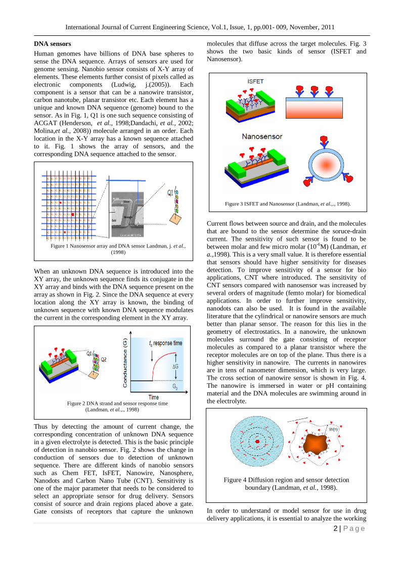
Human genomes have billions of DNA base spheres to sense the DNA sequence. Arrays of sensors are used for genome sensing. Nanobio sensor consists of X-Y array of elements. These elements further consist of pixels called as electronic components (Ludwig, j.(2005)). Each component is a sensor that can be a nanowire transistor, carbon nanotube, planar transistor etc. Each element has a unique and known DNA sequence (genome) bound to the sensor. As in Fig. 1, Q1 is one such sequence consisting of ACGAT (Henderson, et al., 1998;Dandachi, et al., 2002; Molina,et al., 2008)) molecule arranged in an order. Each location in the X-Y array has a known sequence attached to it. Fig. 1 shows the array of sensors, and the corresponding DNA sequence attached to the sensor. When an unknown DNA sequence is introduced into the XY array, the unknown sequence finds its conjugate in the XY array and binds with the DNA sequence present on the array as shown in Fig. 2. Since the DNA sequence at every location along the XY array is known, the binding of unknown sequence with known DNA sequence modulates the current in the corresponding element in the XY array. Thus by detecting the amount of current change, the corresponding concentration of unknown DNA sequence in a given electrolyte is detected. This is the basic principle of detection in nanobio sensor. Fig. 2 shows the change in conduction of sensors due to detection of unknown sequence. There are different kinds of nanobio sensors such as Chem FET, IsFET, Nanowire, Nanosphere, Nanodots and Carbon Nano Tube (CNT). Sensitivity is one of the major parameter that needs to be considered to select an appropriate sensor for drug delivery. Sensors consist of source and drain regions placed above a gate. Gate consists of receptors that capture the unknown

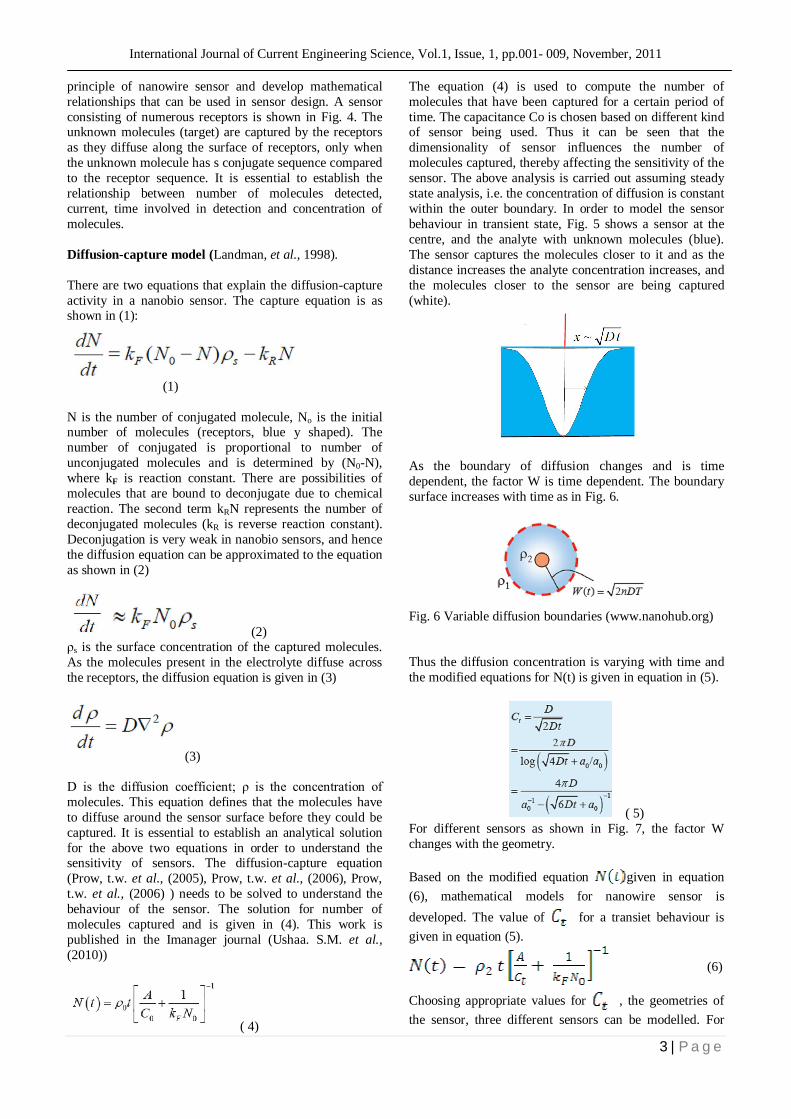
molecules that diffuse across the target molecules. Fig. 3 shows the two basic kinds of sensor (ISFET and Nanosensor).

Current flows between source and drain, and the molecules that are bound to the sensor determine the soruce-drain current. The sensitivity of such sensor is found to be between molar and few micro molar (10-6M) (Landman, et a.,1998). This is a very small value. It is therefore essential that sensors should have higher sensitivity for diseases detection. To improve sensitivity of a sensor for bio applications, CNT where introduced. The sensitivity of CNT sensors compared with nanosensor was increased by several orders of magnitude (femto molar) for biomedical applications. In order to further improve sensitivity, nanodots can also be used. It is found in the available literature that the cylindrical or nanowire sensors are much better than planar sensor. The reason for this lies in the geometry of electrostatics. In a nanowire, the unknown molecules surround the gate consisting of receptor molecules as compared to a planar transistor where the receptor molecules are on top of the plane. Thus there is a higher sensitivity in nanowire. The currents in nanowires are in tens of nanometer dimension, which is very large. The cross section of nanowire sensor is shown in Fig. 4. The nanowire is immersed in water or pH containing material and the DNA molecules are swimming around in the electrolyte. In order to understand or model sensor for use in drug delivery applications, it is essential to analyze the working

Figure 1 Nanosensor array and DNA sensor Landman, j. et al.,

(1998)

Figure 2 DNA strand and sensor response time (Landman, et al.,., 1998)

Figure 3 ISFET and Nanosensor (Landman, et al.,., 1998).

Figure 4 Diffusion region and sensor detection boundary (Landman, et al., 1998).


3 | P a g e

principle of nanowire sensor and develop mathematical relationships that can be used in sensor design. A sensor consisting of numerous receptors is shown in Fig. 4. The unknown molecules (target) are captured by the receptors as they diffuse along the surface of receptors, only when the unknown molecule has s conjugate sequence compared to the receptor sequence. It is essential to establish the relationship between number of molecules detected, current, time involved in detection and concentration of molecules. Diffusion-capture model (Landman, et al., 1998). There are two equations that explain the diffusion-capture activity in a nanobio sensor. The capture equation is as shown in (1):

(1)

N is the number of conjugated molecule, No is the initial number of molecules (receptors, blue y shaped). The number of conjugated is proportional to number of unconjugated molecules and is determined by (N0-N), where kF is reaction constant. There are possibilities of molecules that are bound to deconjugate due to chemical reaction. The second term kRN represents the number of deconjugated molecules (kR is reverse reaction constant). Deconjugation is very weak in nanobio sensors, and hence the diffusion equation can be approximated to the equation as shown in (2)

(2) ρs is the surface concentration of the captured molecules. As the molecules present in the electrolyte diffuse across the receptors, the diffusion equation is given in (3)

(3) D is the diffusion coefficient; ρ is the concentration of molecules. This equation defines that the molecules have to diffuse around the sensor surface before they could be captured. It is essential to establish an analytical solution for the above two equations in order to understand the sensitivity of sensors. The diffusion-capture equation (Prow, t.w. et al., (2005), Prow, t.w. et al., (2006), Prow, t.w. et al., (2006) ) needs to be solved to understand the behaviour of the sensor. The solution for number of molecules captured and is given in (4). This work is published in the Imanager journal (Ushaa. S.M. et al., (2010))

( 4)

The equation (4) is used to compute the number of molecules that have been captured for a certain period of time. The capacitance Co is chosen based on different kind of sensor being used. Thus it can be seen that the dimensionality of sensor influences the number of molecules captured, thereby affecting the sensitivity of the sensor. The above analysis is carried out assuming steady state analysis, i.e. the concentration of diffusion is constant within the outer boundary. In order to model the sensor behaviour in transient state, Fig. 5 shows a sensor at the centre, and the analyte with unknown molecules (blue). The sensor captures the molecules closer to it and as the distance increases the analyte concentration increases, and the molecules closer to the sensor are being captured (white).

As the boundary of diffusion changes and is time dependent, the factor W is time dependent. The boundary surface increases with time as in Fig. 6.

Fig. 6 Variable diffusion boundaries (www.nanohub.org)

Thus the diffusion concentration is varying with time and the modified equations for N(t) is given in equation in (5).

( 5) For different sensors as shown in Fig. 7, the factor W changes with the geometry. Based on the modified equation given in equation (6), mathematical models for nanowire sensor is developed. The value of for a transiet behaviour is given in equation (5).

(6)

Choosing appropriate values for , the geometries of the sensor, three different sensors can be modelled. For


4 | P a g e

different sensors as shown in Fig. 7, the factor changes with the geometry. Experimental setup and sensor characterization Based on the mathematical models discussed, biosensor tool available in Nanohub.org is used for simulation of ISFET, nanowire and nanosphere. For a biosensor the most important parameters that are required are :

Size of micro channel: 5mm x 0.5mm x 50um Flow rate of fluid in the channel: 0.15ml/h Concentration of antigens in fluid:

2⋅10−15⋅6⋅1023≈109 Number of antigens through channel per

hour:1.5x10-4x109 ~ 105 (~ 42 per second) Total area occupied by Antibodies: 5mmx0.5mm

~ 25x10-7m2 Area of one Si NW occupied by Antibodies

(Assumption: r~10nm, l~2um): 2πrl ~ 1.26x10-15 m2

Target receptor conjugation Type of antigen: DNA Ratio between total occupied area and Si NW:

2x109 Mean time between one antigen reacts with one

antibody on the Si NW: <3 minutes

Based on the above parameters, the parameters in the biosensor lab is developed and the models available in the sensor lab are simulated. Fig. 8 shows the experimental setup using the biosensors lab for simulating three different sensors.

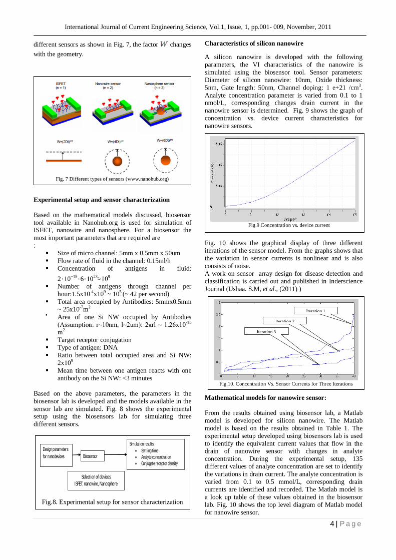
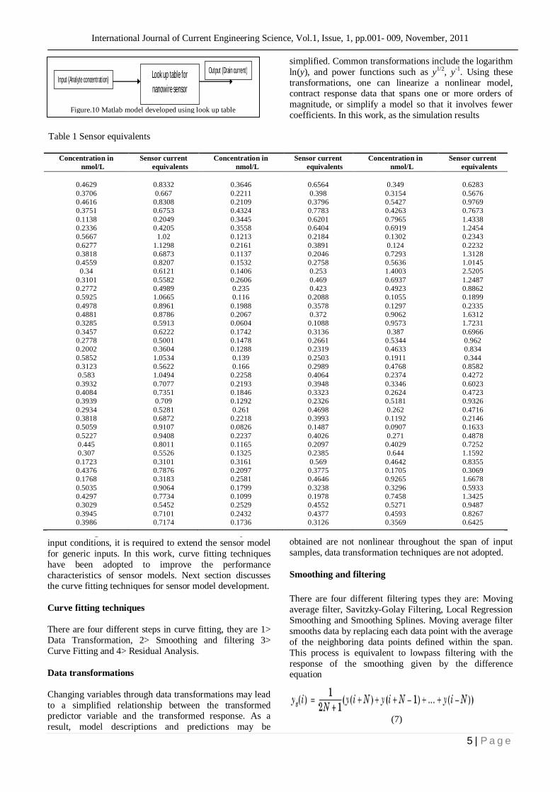
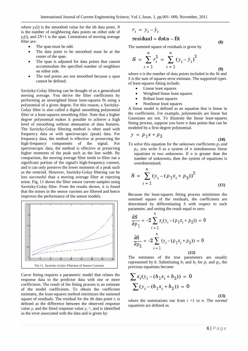
Characteristics of silicon nanowire A silicon nanowire is developed with the following parameters, the VI characteristics of the nanowire is simulated using the biosensor tool. Sensor parameters: Diameter of silicon nanowire: 10nm, Oxide thickness: 5nm, Gate length: 50nm, Channel doping: 1 e+21 /cm3. Analyte concentration parameter is varied from 0.1 to 1 nmol/L, corresponding changes drain current in the nanowire sensor is determined. Fig. 9 shows the graph of concentration vs. device current characteristics for nanowire sensors. Fig. 10 shows the graphical display of three different iterations of the sensor model. From the graphs shows that the variation in sensor currents is nonlinear and is also consists of noise. A work on sensor array design for disease detection and classification is carried out and published in Inderscience Journal (Ushaa. S.M, et al., (2011) ) Mathematical models for nanowire sensor: From the results obtained using biosensor lab, a Matlab model is developed for silicon nanowire. The Matlab model is based on the results obtained in Table 1. The experimental setup developed using biosensors lab is used to identify the equivalent current values that flow in the drain of nanowire sensor with changes in analyte concentration. During the experimental setup, 135 different values of analyte concentration are set to identify the variations in drain current. The analyte concentration is varied from 0.1 to 0.5 mmol/L, corresponding drain currents are identified and recorded. The Matlab model is a look up table of these values obtained in the biosensor lab. Fig. 10 shows the top level diagram of Matlab model for nanowire sensor.

Design parameters for nanodevices Biosensor

Selection of devices ISFET, nanowire, Nanosphere

Simulation results: Settling time Analyte concentration Conjugate receptor density

Fig.8. Experimental setup for sensor characterization

Fig.9 Concentration vs. device current

Iteration 1

Iteration 2

Iteration 3

Fig.10. Concentration Vs. Sensor Currents for Three Iterations

Fig. 7 Different types of sensors (www.nanohub.org)


5 | P a g e

In order to generalize the sensor models for all possible input conditions, it is required to extend the sensor model for generic inputs. In this work, curve fitting techniques have been adopted to improve the performance characteristics of sensor models. Next section discusses the curve fitting techniques for sensor model development. Curve fitting techniques There are four different steps in curve fitting, they are 1> Data Transformation, 2> Smoothing and filtering 3> Curve Fitting and 4> Residual Analysis. Data transformations Changing variables through data transformations may lead to a simplified relationship between the transformed predictor variable and the transformed response. As a result, model descriptions and predictions may be

simplified. Common transformations include the logarithm ln(y), and power functions such as y1/2, y-1. Using these transformations, one can linearize a nonlinear model, contract response data that spans one or more orders of magnitude, or simplify a model so that it involves fewer coefficients. In this work, as the simulation results

obtained are not nonlinear throughout the span of input samples, data transformation techniques are not adopted. Smoothing and filtering There are four different filtering types they are: Moving average filter, Savitzky-Golay Filtering, Local Regression Smoothing and Smoothing Splines. Moving average filter smooths data by replacing each data point with the average of the neighboring data points defined within the span. This process is equivalent to lowpass filtering with the response of the smoothing given by the difference equation

(7)

Look up table for nanowire sensor

Input (Analyte concentration) Output (Drain current)

Figure.10 Matlab model developed using look up table

Table 1 Sensor equivalents

Concentration in nmol/L

Sensor current equivalents





0.4629

0.8332

0.3646

0.6564

0.349

0.6283

0.3706 0.667 0.2211 0.398 0.3154 0.5676 0.4616 0.8308 0.2109 0.3796 0.5427 0.9769 0.3751 0.6753 0.4324 0.7783 0.4263 0.7673 0.1138 0.2049 0.3445 0.6201 0.7965 1.4338 0.2336 0.4205 0.3558 0.6404 0.6919 1.2454 0.5667 1.02 0.1213 0.2184 0.1302 0.2343 0.6277 1.1298 0.2161 0.3891 0.124 0.2232 0.3818 0.6873 0.1137 0.2046 0.7293 1.3128 0.4559 0.8207 0.1532 0.2758 0.5636 1.0145

0.34 0.6121 0.1406 0.253 1.4003 2.5205 0.3101 0.5582 0.2606 0.469 0.6937 1.2487 0.2772 0.4989 0.235 0.423 0.4923 0.8862 0.5925 1.0665 0.116 0.2088 0.1055 0.1899 0.4978 0.8961 0.1988 0.3578 0.1297 0.2335 0.4881 0.8786 0.2067 0.372 0.9062 1.6312 0.3285 0.5913 0.0604 0.1088 0.9573 1.7231 0.3457 0.6222 0.1742 0.3136 0.387 0.6966 0.2778 0.5001 0.1478 0.2661 0.5344 0.962 0.2002 0.3604 0.1288 0.2319 0.4633 0.834 0.5852 1.0534 0.139 0.2503 0.1911 0.344 0.3123 0.5622 0.166 0.2989 0.4768 0.8582 0.583 1.0494 0.2258 0.4064 0.2374 0.4272 0.3932 0.7077 0.2193 0.3948 0.3346 0.6023 0.4084 0.7351 0.1846 0.3323 0.2624 0.4723 0.3939 0.709 0.1292 0.2326 0.5181 0.9326 0.2934 0.5281 0.261 0.4698 0.262 0.4716 0.3818 0.6872 0.2218 0.3993 0.1192 0.2146 0.5059 0.9107 0.0826 0.1487 0.0907 0.1633 0.5227 0.9408 0.2237 0.4026 0.271 0.4878 0.445 0.8011 0.1165 0.2097 0.4029 0.7252 0.307 0.5526 0.1325 0.2385 0.644 1.1592 0.1723 0.3101 0.3161 0.569 0.4642 0.8355 0.4376 0.7876 0.2097 0.3775 0.1705 0.3069 0.1768 0.3183 0.2581 0.4646 0.9265 1.6678 0.5035 0.9064 0.1799 0.3238 0.3296 0.5933 0.4297 0.7734 0.1099 0.1978 0.7458 1.3425 0.3029 0.5452 0.2529 0.4552 0.5271 0.9487 0.3945 0.7101 0.2432 0.4377 0.4593 0.8267 0.3986 0.7174 0.1736 0.3126 0.3569 0.6425


6 | P a g e

where ys(i) is the smoothed value for the ith data point, N is the number of neighboring data points on either side of ys(i), and 2N+1 is the span. Limitations of moving average filter are:

The span must be odd. The data point to be smoothed must be at the

center of the span. The span is adjusted for data points that cannot

accommodate the specified number of neighbors on either side.

The end points are not smoothed because a span cannot be defined.

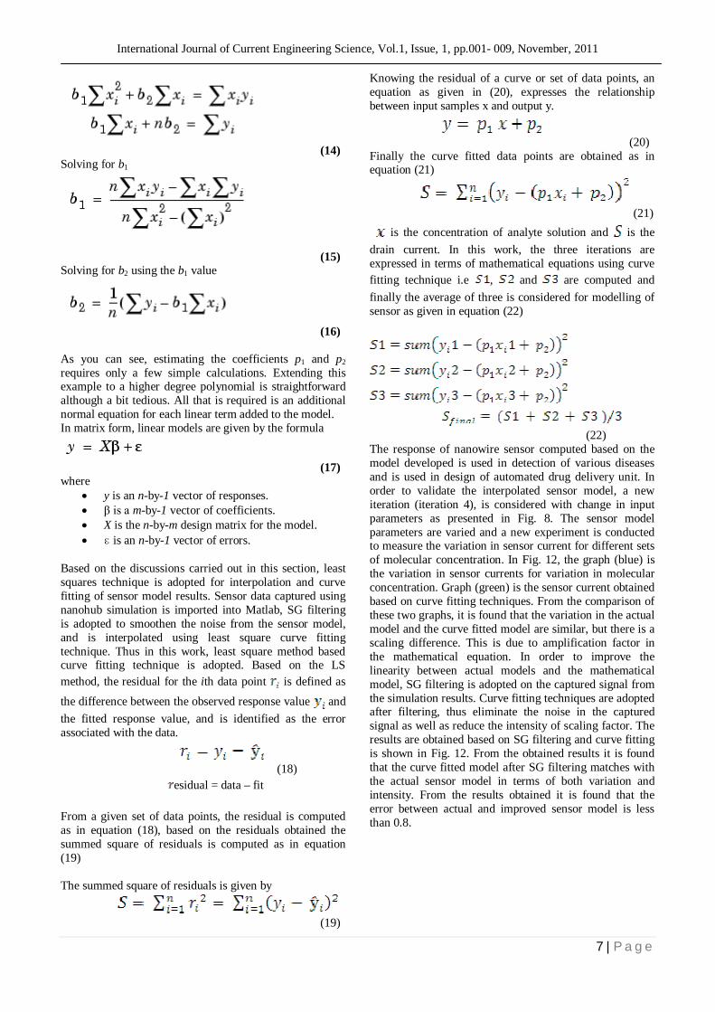
Savitzky-Golay filtering can be thought of as a generalized moving average. You derive the filter coefficients by performing an unweighted linear least-squares fit using a polynomial of a given degree. For this reason, a Savitzky-Golay filter is also called a digital smoothing polynomial filter or a least-squares smoothing filter. Note that a higher degree polynomial makes it possible to achieve a high level of smoothing without attenuation of data features. The Savitzky-Golay filtering method is often used with frequency data or with spectroscopic (peak) data. For frequency data, the method is effective at preserving the high-frequency components of the signal. For spectroscopic data, the method is effective at preserving higher moments of the peak such as the line width. By comparison, the moving average filter tends to filter out a significant portion of the signal's high-frequency content, and it can only preserve the lower moments of a peak such as the centroid. However, Savitzky-Golay filtering can be less successful than a moving average filter at rejecting noise. Fig. 11 shows the filter sensor current samples using Savitzky-Golay filter. From the results shown, it is found that the noises in the sensor currents are filtered and hence improves the performance of the sensor models. Curve fitting requires a parametric model that relates the response data to the predictor data with one or more coefficients. The result of the fitting process is an estimate of the model coefficients. To obtain the coefficient estimates, the least-squares method minimizes the summed square of residuals. The residual for the ith data point ri is defined as the difference between the observed response value yi and the fitted response value yi ^, and is identified as the error associated with the data and is given by:

(8) The summed square of residuals is given by

(9) where n is the number of data points included in the fit and S is the sum of squares error estimate. The supported types of least-squares fitting include:

Linear least squares Weighted linear least squares Robust least squares Nonlinear least squares

A linear model is defined as an equation that is linear in the coefficients. For example, polynomials are linear but Gaussians are not. To illustrate the linear least-squares fitting process, suppose you have n data points that can be modeled by a first-degree polynomial.

(10) To solve this equation for the unknown coefficients p1 and

p2, you write S as a system of n simultaneous linear equations in two unknowns. If n is greater than the number of unknowns, then the system of equations is overdetermined.

(11) Because the least-squares fitting process minimizes the summed square of the residuals, the coefficients are determined by differentiating S with respect to each parameter, and setting the result equal to zero.

(12)

The estimates of the true parameters are usually represented by b. Substituting b1 and b2 for p1 and p2, the previous equations become

(13)

where the summations run from i =1 to n. The normal equations are defined as

Fig.11. Savitzky-Golay Filtering of Sensor Currents


7 | P a g e

(14)

Solving for b1

(15) Solving for b2 using the b1 value

(16)

As you can see, estimating the coefficients p1 and p2 requires only a few simple calculations. Extending this example to a higher degree polynomial is straightforward although a bit tedious. All that is required is an additional normal equation for each linear term added to the model. In matrix form, linear models are given by the formula

(17)

where y is an n-by-1 vector of responses. β is a m-by-1 vector of coefficients. X is the n-by-m design matrix for the model. ɛ is an n-by-1 vector of errors.

Based on the discussions carried out in this section, least squares technique is adopted for interpolation and curve fitting of sensor model results. Sensor data captured using nanohub simulation is imported into Matlab, SG filtering is adopted to smoothen the noise from the sensor model, and is interpolated using least square curve fitting technique. Thus in this work, least square method based curve fitting technique is adopted. Based on the LS method, the residual for the ith data point is defined as

the difference between the observed response value and the fitted response value, and is identified as the error associated with the data.

(18)

esidual = data – fit

From a given set of data points, the residual is computed as in equation (18), based on the residuals obtained the summed square of residuals is computed as in equation (19) The summed square of residuals is given by

(19)

Knowing the residual of a curve or set of data points, an equation as given in (20), expresses the relationship between input samples x and output y.

(20) Finally the curve fitted data points are obtained as in equation (21)

(21)

is the concentration of analyte solution and is the drain current. In this work, the three iterations are expressed in terms of mathematical equations using curve fitting technique i.e , and are computed and finally the average of three is considered for modelling of sensor as given in equation (22)

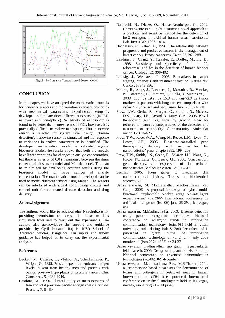
(22) The response of nanowire sensor computed based on the model developed is used in detection of various diseases and is used in design of automated drug delivery unit. In order to validate the interpolated sensor model, a new iteration (iteration 4), is considered with change in input parameters as presented in Fig. 8. The sensor model parameters are varied and a new experiment is conducted to measure the variation in sensor current for different sets of molecular concentration. In Fig. 12, the graph (blue) is the variation in sensor currents for variation in molecular concentration. Graph (green) is the sensor current obtained based on curve fitting techniques. From the comparison of these two graphs, it is found that the variation in the actual model and the curve fitted model are similar, but there is a scaling difference. This is due to amplification factor in the mathematical equation. In order to improve the linearity between actual models and the mathematical model, SG filtering is adopted on the captured signal from the simulation results. Curve fitting techniques are adopted after filtering, thus eliminate the noise in the captured signal as well as reduce the intensity of scaling factor. The results are obtained based on SG filtering and curve fitting is shown in Fig. 12. From the obtained results it is found that the curve fitted model after SG filtering matches with the actual sensor model in terms of both variation and intensity. From the results obtained it is found that the error between actual and improved sensor model is less than 0.8.


8 | P a g e

CONCLUSION In this paper, we have analyzed the mathematical models for nanowire sensors and the variation in sensor properties with geometrical parameters. Experimental setup is developed to simulate three different nanosensors (ISFET, nanowire and nanosphere). Sensitivity of nanosphere is found to be better than nanowire and ISFET, however, it is practically difficult to realize nanosphere. Thus nanowire sensor is selected for system level design (disease detection), nanowire sensor is simulated and its response to variations in analyte concentration is identified. The developed mathematical model is validated against biosensor model, the results shows that both the models have linear variations for changes in analyte concentration, but there is an error of 0.8 (maximum), between the drain currents of biosensor model and Matlab model. This can be minimized by developing accurate results using the biosensor model for large number of analyte concentration. The mathematical model developed can be used to model different sensors using Matlab. The sensors can be interfaced with signal conditioning circuits and control unit for automated disease detection and drug delivery. Acknowledgement The authors would like to acknowledge Nanohub.org for providing permission to access the biosensor labs simulation tools and to carry out the experiments. The authors also acknowledge the support and guidance provided by Cyril Prasanna Raj P., MSR School of Advanced Studies, Bangalore. His inputs and timely guidance has helped us to carry out the experimental analysis. References

Beckett, M., Cazares, L., Vlahou, A., Schellhammer, P.,

Wright, G., 1995. Prostate-specific membrane antigen levels in sera from healthy men and patients with benign prostate hyperplasia or prostate cancer. Clin. Cancer res. 5, 4034-4040.

Catalona, W., 1996. Clinical utility of measurements of free and total prostate-specific antigen (psa): a review. Prostate, 7, 64-69.

Dandachi, N., Dietze, O., Hauser-kronberger, C., 2002. Chromogenic in situ hybridization: a novel approach to a practical and sensitive method for the detection of her2 oncogene in archival human breast carcinoma. Lab. Invest. 82, 1007–1014.

Henderson, C., Patek, A., 1998. The relationship between prognostic and predictive factors in the management of breast cancer. Breast cancer res. Treat. 52, 261-288.

Landman, J., Chang, Y., Kavaler, E., Droller, M., Liu, B., 1998. Sensitivity and specificity of nmp- 22, telomerase, and bta in the detection of human bladder cancer. Urology. 52, 398-402.

Ludwig, J., Weinstein, J., 2005. Biomarkers in cancer staging, prognosis and treatment selection. Nature rev. Cancer, 5, 845-856.

Molina, R., Auge, J., Escudero, J., Marrades, R., Vinolas, N., Carcereny, E., Ramirez, J., Filella, X. Mucins ca., 2008. 125, ca 19.9, ca 15.3 and tag-72.3 as tumor markers in patients with lung cancer: comparison with cyfra 21-1, cea, scc and nse. Tumor biol. 29, 371-380.

Prow, T.W., Grebe, R., Merges, C., Smith, J.N., Mcleod, D.S., Leary, J.F., Gerard A. Lutty, G.A., 2006. Novel therapeutic gene regulation by genetic biosensor tethered to magnetic nanoparticles for the detection and treatment of retinopathy of prematurity. Molecular vision 12: 616-625.

Prow, T.W., Rose, W.A., Wang, N., Reece, L.M., Lvov, Y., Leary, J.F., 2005. Biosensor-controlled gene therapy/drug delivery with nanoparticles for nanomedicine" proc. of spie 5692: 199 –208,

Prow, T.W., Smith, J.N., Grebe, R., Salazar, J.H., Wang, N., Kotov, N., Lutty, G., Leary, J.F., 2006. Construction, gene delivery, and expression of dna tethered nanoparticles. Molecular vision 12: 606-615.

Seeman, 2005. From genes to machines: dna nanomechanical devices. Trends in biochemical sciences 30

Ushaa eswaran, M. Madhavilatha, Madhusudhana Rao Ganji., 2006. A proposal for design of hybrid multi-functional implantable biochip using bio-intelligent expert system’ the 2006 international conference on artificial intelligence (icai'06) june 26-29, , las vegas, usa

Ushaa eswaran, M.Madhavilatha, 2009. Disease detection using pattern recognition techniques. National conference on 'emerging trends in information communication technology' (etict-08) held in gitam university, india during 19th & 20th december and is published in gitam journal of information communication technology of vol-2 jan - july 2009 number - 1 (issn 0974-4622) pp 34-37

Ushaa eswaran, madhusudhan rao ganji , jayashankarts, lekha suresh, 2006. Design of implantable vlsi bio-chip. National conference on advanced communication technologies (act-06), 8-9 december.

Ushaa eswaran, Madhusudhana Rao, M.S.Thakur, 2004. Microprocessor based biosensors for determination of toxins and pathogens in restricted areas of human intervention. ic ai’04 ieee sponsored international conference on artificial intelligence held in las vegas, nevada, usa during 21 – 24 june ,.

Fig.12. Perfromance Comparison of Sensor Models


9 | P a g e

Ushaa. S.M., Madhavilatha.M., Madhusudhana Rao Ganji 2011. Design and Analysis of Nanowire Sensor Array for Prostate Cancer Detection" (Submission code: IJNBM-20274) for the International Journal of Nano and Biomaterials (IJNBM). Int. J. Nano and Biomaterials, Vol. 3, No. 3.

Ushaa. S.M., Madhavilatha.M; Madhusudhana Rao Ganji, 2010. Development and validation of matlab models for nanowire sensors for disease detection. i-manager’s journal on future engineering & technology, vol. 6 l no. 2 l

www.nanohub.org

*******

PERFORMANCE IMPROVEMENT OF NANOWIRE SENSOR...

Documents

Transcript of PERFORMANCE IMPROVEMENT OF NANOWIRE SENSOR...