
PERFORMANCE EVALUATION OF SMALL SCALE IRRIGATION …
97
DSpace Institution DSpace Repository http://dspace.org Hydraulic and Water Resources Engineering thesis 2020-03-17 PERFORMANCE EVALUATION OF SMALL SCALE IRRIGATION SCHEME: A CASE STUDY OF BRANTI IRRIGATION SCHEME, SOUTH ACHEFER WOREDA, ETHIOPIA KELEMEWORK, GETACHEW http://hdl.handle.net/123456789/10513 Downloaded from DSpace Repository, DSpace Institution's institutional repository
Transcript of PERFORMANCE EVALUATION OF SMALL SCALE IRRIGATION …
DSpace Institution
DSpace Repository http://dspace.org
Hydraulic and Water Resources Engineering thesis
2020-03-17
PERFORMANCE EVALUATION OF
SMALL SCALE IRRIGATION SCHEME:
A CASE STUDY OF BRANTI
IRRIGATION SCHEME, SOUTH
ACHEFER WOREDA, ETHIOPIA
KELEMEWORK, GETACHEW
http://hdl.handle.net/123456789/10513
Downloaded from DSpace Repository, DSpace Institution's institutional repository
i
BAHIR DAR UNIVERSITY
BAHIR DAR INSTITUTE OF TECHNOLOGY
SCHOOL OF RESEARCH AND POSTGRADUATE STUDIES
FACULTY OF CIVIL AND WATER RESOURCES ENGINEERING
PERFORMANCE EVALUATION OF SMALL SCALE IRRIGATION
SCHEME: A CASE STUDY OF BRANTI IRRIGATION SCHEME, SOUTH
ACHEFER WOREDA, ETHIOPIA
By
Getachew Kelemework
Bahir Dar, Ethiopia
July, 2018
i
PERFORMANCE EVALUATION OF SMALL SCALE IRRIGATION
SCHEME: A CASE STUDY OF BRANTI IRRIGATION SCHEME, SOUTH
ACHEFER WOREDA, ETHIOPIA
GETACHEW KELEMEWORK
A thesis submitted to the school of Research and Graduate Studies of Bahir Dar
Institute of Technology, BDU in partial fulfilment of the requirements for the degree
Of
Master of Science in the Engineering Hydrology to Faculty of Civil and Water
Resources Engineering, Bahir Dar Institute of Technology, Bahir Dar University
Advisor Name: Dr. Temsgen Enku
BahirDar, Ethiopia
July 24, 2018

ii

iii

iv
ACKNOWLEDGEMENTS
First and foremost, I would like to offer my deepest thanks to the almighty God for keeping me
inspired and courageous to go through all this work.
I would like to express my deepest appreciation and special thanks to my advisor Dr.Temsgen
Enku for his respect full devotion, precious time and valuable comments to conduct my Thesis
Research work successfully.
I am also indebted to my colleagues for their unrestricted intellectual, material and moral
assistance during the study period.
I am very grateful for South Achefer Woreda Agricultural Office, Ahuri Keltafa Kebele DAs,
ANRS Water Irrigation and Energy Bureau for their Professional material and moral assistance
during my study.
My special thanks go to Ethiopian Road Authority for their financial support to undertake the
study in Bahir Dar University.
Finally, I would like to express my sincere appreciation and gratitude to all of my families for
their encouragement and support during my study.

v
ABSTRACT
In Ethiopia irrigation subsector is chosen as the policy option in stimulating sustainable
economic growth in rural areas. Irrigation development in the country is confronted by many
problems and it performs below its potential. Therefore in this study irrigation scheme
performance assessment is vital to identify performance gaps and to improve scheme
performances. However, the performance of Branti small scale irrigation scheme in South
Achefer Woreda Ahuri Keltafa Kebele was not assessed up to now. Primary and secondary data
were collected in the study. Secondary data from different reports and primary data through
field measurements, key informant interviews and group discussions were collected. For
performance evaluation of the irrigation scheme three farmers’ fields were selected from head,
middle and tail water users. As a result application efficiency (Ea), conveyance efficiency (Ec),
water storage efficiency (Es), deep percolation fraction (DPF) and overall scheme efficiency
were determined and their average values were found to be 17.05%, 84.74%, 50.44%, 82.95%,
and 14.58%, respectively. Evaluation of irrigation water requirement and crop water
requirement of main crops were evaluated using CROPWAT 8. The irrigation water requirement
of onion, pepper and potato grown in the study area are 389.8, 372.4 and 388.9mm/season
respectively. Water delivery performance of the irrigation scheme was 43.74% which result in
56.26 % of reduction of the capacity of the intake canal. Finally structured questionnaires and
group discussions were used to assess the attitude of farmers’ about the performance of their
irrigation scheme. The respondents’ response revealed that the major causes for
underperformance of the scheme are seepage from the headwork and/or canals, sedimentation
and structural failure. Therefore, the conveyance system should be improved through regular
canal cleaning and maintenance of canal structures and constructing flow control gates (canal
gates). In general performance of the irrigation scheme was rated as poor and crop pattern of
the study area was organized in CROPWAT 8.0 model along with necessary data such as
climate, soil and crop data.
Key words; performance, efficiency, water, irrigation, SSI scheme
vi
TABLE OF CONTENTS
ACKNOWLEDGEMENTS ........................................................................................................... iii
ABSTRACT .................................................................................................................................... v
LIST OF ABBREVIATIONS ...................................................................................................... viii
LIST OF TABLES ......................................................................................................................... ix
LIST OF FIGURES ........................................................................................................................ x
1. INTRODUCTION ...................................................................................................................... 1
1.1. Background .......................................................................................................................... 1
1.2. Problem Statement ............................................................................................................... 3
1.3. Objectives ............................................................................................................................. 4
1.3.1. General objective............................................................................................................... 4
1.3.2. Specific Objectives ............................................................................................................ 4
1.4. Research Questions .............................................................................................................. 4
1.5 Significance of the study ....................................................................................................... 5
1.6 Scope of the study ................................................................................................................. 5
2. LITERATURE REVIEW ........................................................................................................... 6
2.1. Overview of Irrigation Development in Africa .................................................................... 6
2.2. Irrigation Developments in Ethiopia .................................................................................... 7
2.3. Evaluating Irrigation Systems and Practices ........................................................................ 9
2.3.1. Irrigation water management ......................................................................................... 9
2.3.2. Performance indicators ................................................................................................ 10
2.4. Irrigation Scheduling .......................................................................................................... 13
3. MATERIALS AND METHODS .............................................................................................. 14
3.1. Description of the study area .............................................................................................. 14
3.1.1. Location ....................................................................................................................... 14
3.1.2. Hydro-meteorological data availability ....................................................................... 15
3.1.3. Soil and topography ..................................................................................................... 18
3.1.4. Description of Branti small-scale irrigation scheme ................................................... 18
3.2. Methodology ...................................................................................................................... 20
3.2.1. Data Collection and analysis ....................................................................................... 20
3.2.2. Determination of the Amount of Water Applied to the Fields .................................... 26
3.2.3.To assess water scarcity and irrigation water management of the irrigation scheme...26

vii
3.2.4. Scheme Performance Evaluation ................................................................................. 27
3.2.5. Sustainability and Water Delivery Performance evaluation ........................................ 31
3.3. Institutional Aspect ............................................................................................................ 33
4. RESULTS AND DISCUSSION ............................................................................................ 34
4.1. Soil Characteristics ............................................................................................................. 34
4.2. Soil data analysis results .................................................................................................... 34
4.2.1 .Particle size distribution (Texture) .............................................................................. 34
4.2.2 Determination of bulk density, field capacity and permanent wilting point ................ 35
4.3. Reference evapo-transpiration (ETO) ................................................................................ 36
4.4. Crop and irrigation water requirements of major crops in the study area .......................... 37
4.5. Irrigation Scheduling .......................................................................................................... 38
4.6. Performance Evaluations.................................................................................................... 40
4.6.1. Application Efficiency ................................................................................................. 40
4.6.2. Conveyance Efficiency ................................................................................................ 43
4.6.3. Storage efficiency ........................................................................................................ 45
4.6.4. Deep Percolation Ratio ................................................................................................ 46
4.6.5. Overall Scheme Efficiency .......................................................................................... 46
4.7. Water Delivery Performance .............................................................................................. 47
4.8. Sustainability of the Irrigation scheme .............................................................................. 47
4.9. Institutional aspect and farmer’s perception about the irrigation scheme .......................... 48
4.9.2. Sustainability of the Scheme ....................................................................................... 51
4.9.3. Conflict and Conflict Resolution Mechanisms ............................................................ 53
4.9.4. Support Service............................................................................................................ 54
5. CONCLUSION AND RECOMMENDATION ........................................................................ 55
5.1. Conclusion .......................................................................................................................... 55
5.2. Recommendation ................................................................................................................ 56
6. REFERNCES ............................................................................................................................ 57
APPENDIX ................................................................................................................................... 61
APPENDIX 1-TABLE .............................................................................................................. 61
APPENDIX FIGURES-2 .......................................................................................................... 77
APPENDIX-3 QUESTIONER .................................................................................................. 81
viii
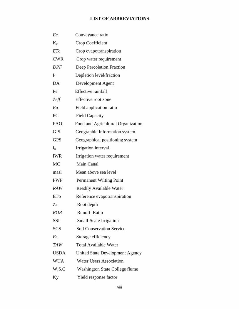
LIST OF ABBREVIATIONS
Ec Conveyance ratio
Kc Crop Coefficient
ETc Crop evapotranspiration
CWR Crop water requirement
DPF Deep Percolation Fraction
P Depletion level/fraction
DA Development Agent
Pe Effective rainfall
Zeff Effective root zone
Ea Field application ratio
FC Field Capacity
FAO Food and Agricultural Organization
GIS Geographic Information system
GPS Geographical positioning system
In Irrigation interval
IWR Irrigation water requirement
MC Main Canal
masl Mean above sea level
PWP Permanent Wilting Point
RAW Readily Available Water
ETo Reference evapotranspiration
Zr Root depth
ROR Runoff Ratio
SSI Small-Scale Irrigation
SCS Soil Conservation Service
Es Storage efficiency
TAW Total Available Water
USDA United State Development Agency
WUA Water Users Association
W.S.C Washington State College flume
Ky Yield response factor
ix
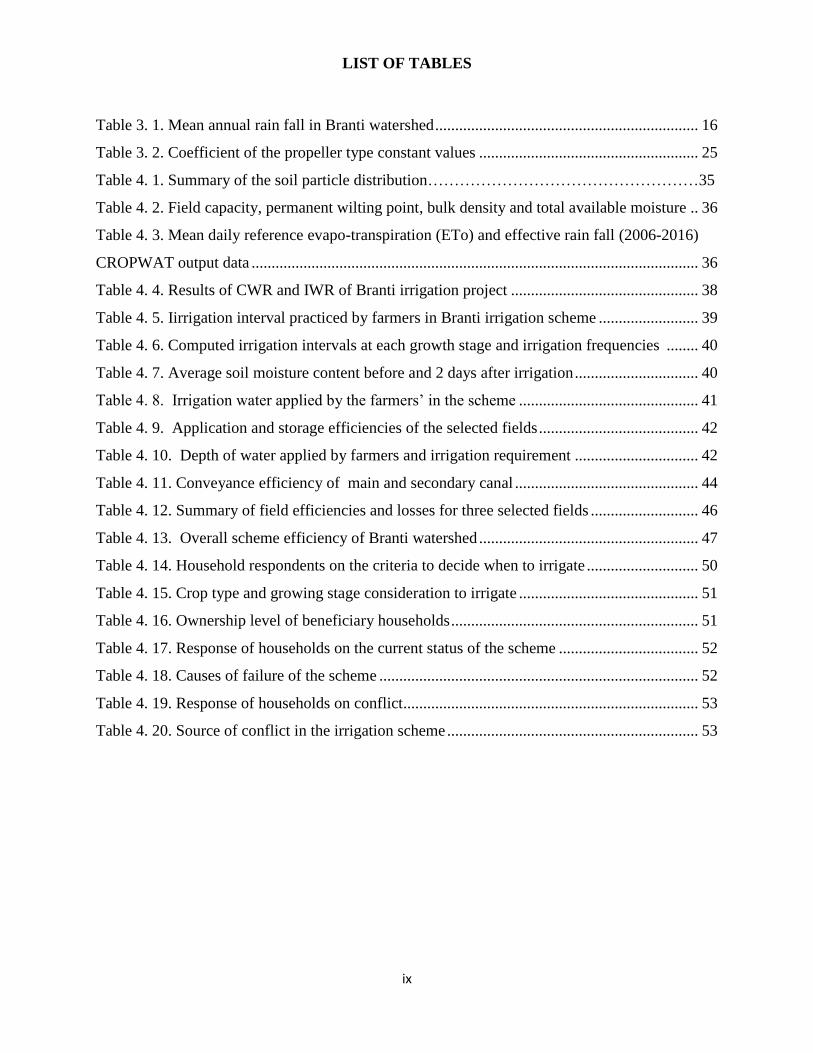
LIST OF TABLES
Table 3. 1. Mean annual rain fall in Branti watershed .................................................................. 16
Table 3. 2. Coefficient of the propeller type constant values ....................................................... 25
Table 4. 1. Summary of the soil particle distribution……………………………………………35
Table 4. 2. Field capacity, permanent wilting point, bulk density and total available moisture .. 36
Table 4. 3. Mean daily reference evapo-transpiration (ETo) and effective rain fall (2006-2016)
CROPWAT output data ................................................................................................................ 36
Table 4. 4. Results of CWR and IWR of Branti irrigation project ............................................... 38
Table 4. 5. Iirrigation interval practiced by farmers in Branti irrigation scheme ......................... 39
Table 4. 6. Computed irrigation intervals at each growth stage and irrigation frequencies ........ 40
Table 4. 7. Average soil moisture content before and 2 days after irrigation ............................... 40
Table 4. 8. Irrigation water applied by the farmers’ in the scheme ............................................. 41
Table 4. 9. Application and storage efficiencies of the selected fields ........................................ 42
Table 4. 10. Depth of water applied by farmers and irrigation requirement ............................... 42
Table 4. 11. Conveyance efficiency of main and secondary canal .............................................. 44
Table 4. 12. Summary of field efficiencies and losses for three selected fields ........................... 46
Table 4. 13. Overall scheme efficiency of Branti watershed ....................................................... 47
Table 4. 14. Household respondents on the criteria to decide when to irrigate ............................ 50
Table 4. 15. Crop type and growing stage consideration to irrigate ............................................. 51
Table 4. 16. Ownership level of beneficiary households .............................................................. 51
Table 4. 17. Response of households on the current status of the scheme ................................... 52
Table 4. 18. Causes of failure of the scheme ................................................................................ 52
Table 4. 19. Response of households on conflict .......................................................................... 53
Table 4. 20. Source of conflict in the irrigation scheme ............................................................... 53
x
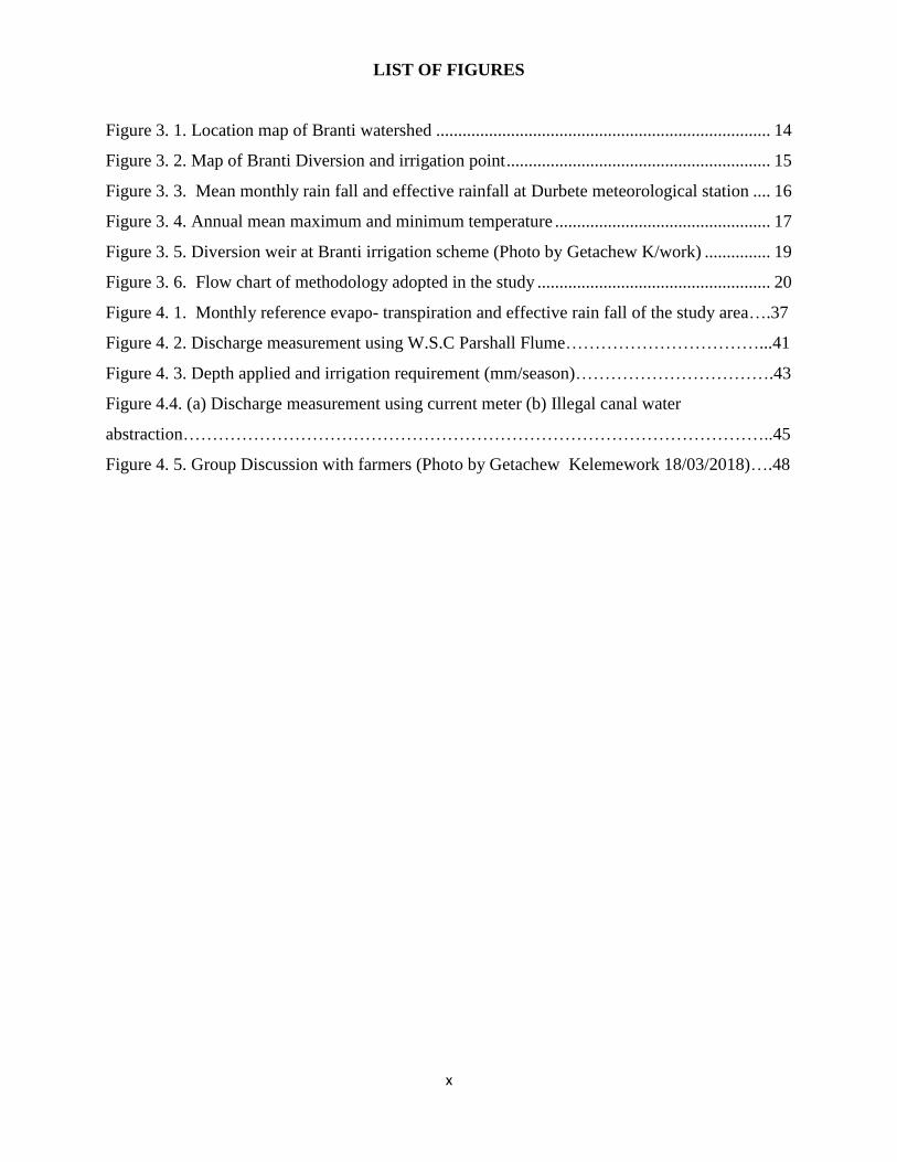
LIST OF FIGURES
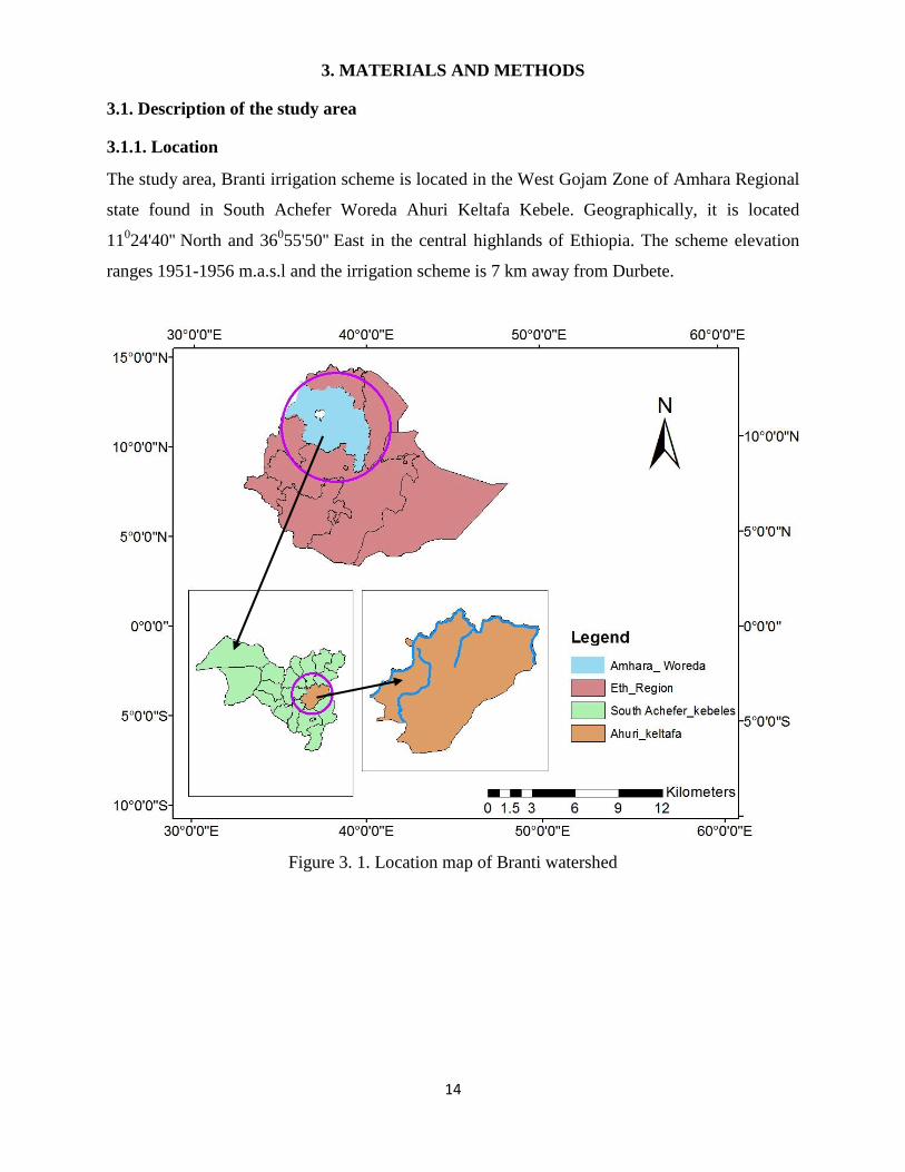
Figure 3. 1. Location map of Branti watershed ............................................................................ 14
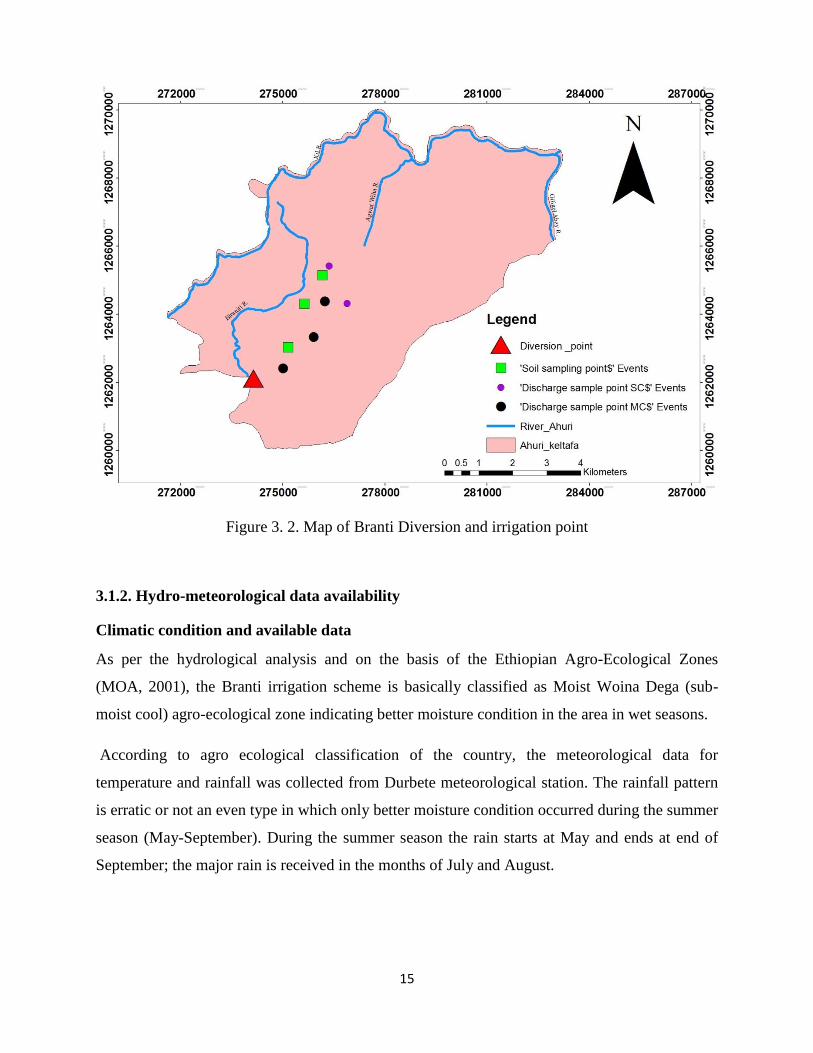
Figure 3. 2. Map of Branti Diversion and irrigation point ............................................................ 15
Figure 3. 3. Mean monthly rain fall and effective rainfall at Durbete meteorological station .... 16
Figure 3. 4. Annual mean maximum and minimum temperature ................................................. 17
Figure 3. 5. Diversion weir at Branti irrigation scheme (Photo by Getachew K/work) ............... 19
Figure 3. 6. Flow chart of methodology adopted in the study ..................................................... 20
Figure 4. 1. Monthly reference evapo- transpiration and effective rain fall of the study area….37
Figure 4. 2. Discharge measurement using W.S.C Parshall Flume……………………………...41
Figure 4. 3. Depth applied and irrigation requirement (mm/season)…………………………….43
Figure 4.4. (a) Discharge measurement using current meter (b) Illegal canal water
abstraction………………………………………………………………………………………..45
Figure 4. 5. Group Discussion with farmers (Photo by Getachew Kelemework 18/03/2018)….48

1
1. INTRODUCTION
1.1. Background
Irrigation is an application of water that supplies the soil moisture deficit. A reliable and suitable
irrigation water supply can result in improvements in agricultural production and assure the
economic vitality. Many civilizations have risen on irrigated agriculture; these provide basis for
their society and enhance food security of their people. Estimates indicate that as little as 15-20%
of the worldwide total cultivated area is irrigated and comparing irrigated and non-irrigated
yields in some areas, this relatively small fraction of agriculture contributes as much as 30-40%
of gross agricultural output (FAO, 1989).
Irrigation is one means which agricultural production can be increased to meet the growing
demands for food in Ethiopia (Awlachew et al., 2010). A study also indicated that one of the best
alternatives to consider reliable and sustainable food security development in order to expanding
irrigation development on various scales through river diversion, constructing micro dams, water
harvesting structures, etc. (Lambisso, 2005).
Ethiopia has an important opportunity in water-led development which is endowed with
abundant water resources. The country has 12 river basins with an annual runoff volume of 124
billion meter cube of water and 30 billion meter cube ground water potential (EPCC, 2015). The
total potential irrigable land in country is estimated to be around 5.3 million ha (MoWR, 2014).
But current irrigable area of the country is 640,000 ha (IWMI, 2010). This means that a
significant portion of irrigable land in Ethiopia is currently not irrigated. This means that there
are potential opportunities to vastly increase the amount of irrigated land in the country.
Like Ethiopia, Amhara region have abundant water resources in the country. The annual runoff
in the region is estimated to be 60 billion meter cube with water resources per capita of 3,570 m3
(Melkamu, 1996). A region is divided mainly by three river basins namely the Abbay, Tekezze
and Awash drainage basins. This region has vast potential for irrigation development. Estimated
potential land for large and medium scale irrigation of the region is about 650,000 - 700,000 ha
and for small scale irrigation is about 200,000 - 250,000 ha, indicates the magnitude of water
resources available for development (BCEOM, 1999).
The study site is located within Tana sub basin, which is a tributary to Gilgel Abay river basin.
As before the establishment of the project, the irrigation activity in scheme was depend on
2
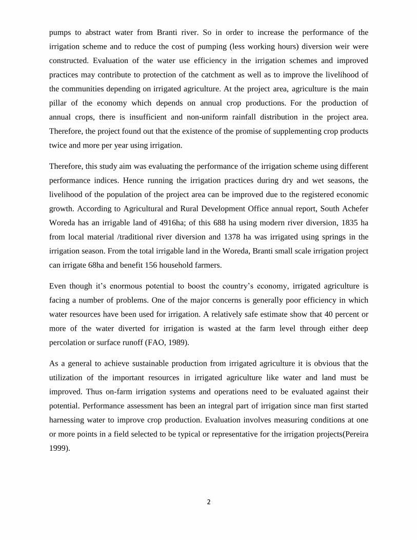
pumps to abstract water from Branti river. So in order to increase the performance of the
irrigation scheme and to reduce the cost of pumping (less working hours) diversion weir were
constructed. Evaluation of the water use efficiency in the irrigation schemes and improved
practices may contribute to protection of the catchment as well as to improve the livelihood of
the communities depending on irrigated agriculture. At the project area, agriculture is the main
pillar of the economy which depends on annual crop productions. For the production of
annual crops, there is insufficient and non-uniform rainfall distribution in the project area.
Therefore, the project found out that the existence of the promise of supplementing crop products
twice and more per year using irrigation.
Therefore, this study aim was evaluating the performance of the irrigation scheme using different
performance indices. Hence running the irrigation practices during dry and wet seasons, the
livelihood of the population of the project area can be improved due to the registered economic
growth. According to Agricultural and Rural Development Office annual report, South Achefer
Woreda has an irrigable land of 4916ha; of this 688 ha using modern river diversion, 1835 ha
from local material /traditional river diversion and 1378 ha was irrigated using springs in the
irrigation season. From the total irrigable land in the Woreda, Branti small scale irrigation project
can irrigate 68ha and benefit 156 household farmers.
Even though it’s enormous potential to boost the country’s economy, irrigated agriculture is
facing a number of problems. One of the major concerns is generally poor efficiency in which
water resources have been used for irrigation. A relatively safe estimate show that 40 percent or
more of the water diverted for irrigation is wasted at the farm level through either deep
percolation or surface runoff (FAO, 1989).
As a general to achieve sustainable production from irrigated agriculture it is obvious that the
utilization of the important resources in irrigated agriculture like water and land must be
improved. Thus on-farm irrigation systems and operations need to be evaluated against their
potential. Performance assessment has been an integral part of irrigation since man first started
harnessing water to improve crop production. Evaluation involves measuring conditions at one
or more points in a field selected to be typical or representative for the irrigation projects(Pereira
1999).

3
1.2. Problem Statement
Ethiopia has an opportunity in water-led development but it needs to address critical challenges
in the planning, design, delivery and maintenance of irrigation systems to exploit its full
potential. Hence irrigation has the major importance in terms of agricultural production and food
supply, the income of rural society and public investment for rural development show increased
economic vitality trend. But the dry season rain is considered inadequate; i.e. there is notable
variation in terms of onset, distribution and withdrawal from year to year affecting crop
production in general and crop productivity in particular. So to sustain this seasonal variation,
irrigation is paramount that plays significant role in the production of agricultural products.
Studies shows that there is wide spread dissatisfaction with the performance of irrigation projects
in developing countries (Behailu et al., 2004).The reason that irrigation projects typically
perform far below their potential is due to sedimentation problems, leaky canals and
malfunctioning structures because of delayed maintenance leading to low water-use efficiency
and low yields are some of the commonly expressed problems (Behailu et al., 2004). .
Poor management of available water for irrigation at the canal system and farm level has also led
to a range of problems and further aggravated water availability and has reduced the
benefits of irrigation investments (FAO, 1996). Irrigation projects have the potential to degrade
the land, soil and wastage of valuable resource (water) if they are mismanaged. In recognition of
both the benefit and hazards assessment, evaluation of irrigation schemes has now become a
paramount importance not only to point out where the problem lies but also helps to identify
alternatives that may be both effective and feasible in improving system performance.
Besides the poor performance of irrigation projects, evaluation of irrigation projects is not
common: lack of knowledge and tools used to assess the performance of projects adds to the
problem. But now a day’s International water management institute has developed a set of
comparative indicators that are used to asses internal performance indicators of irrigation system
which are helpful to determine the condition of the system and proper functioning of its
elements.
As a general farmers use local materials to divert water from the canal to their target point and
use un-manageable irrigation frequency which result in poor water management. As water
4
distribution in the scheme is handled by farmers and water users association without knowing
either the volumes of water delivered or the duration of water supplied to each irrigator.
Inefficient water use and inadequate water management both at farm and scheme level mean
much less area can be irrigated than planned and agricultural production falls well below target
(Mehta, 1994).
So, evaluating the performance of Branti small-scale irrigation scheme is important to know the
efficiency of the irrigation scheme and give valuable recommendations to improve irrigation
water management system and also will solve conflict between water users.
1.3. Objectives
1.3.1. General objective
The general objective is to assess and evaluate the performance of Branti small-scale irrigation
scheme.
1.3.2. Specific Objectives
The specific objectives of the study:
To assess irrigation efficiency (conveyance and application) of the irrigation scheme
To assess water delivery performance of the irrigation scheme
To assess water scarcity and irrigation water management of the irrigation scheme
To assess farmers perception about their irrigation scheme
1.4. Research Questions
The following research questions were addressed in this study:
How much is the efficiency of the scheme actually performed?
Are farmers actually deliver and apply irrigation water in the right amount and time in the
irrigation scheme?
What is the farmers’ perception about their irrigation scheme?

5
1.5 Significance of the study
Performance evaluation of Branti irrigation scheme has a great importance to point out the
problems and to address the future system management in the study area. The study is assisting
to distinguish whether the targets and objectives are being met or not and also provides system
managers, farmers and policy makers a better understanding of how the system operates. It also
used to identify the strengths, weaknesses and specific areas needed to be improved.
It is of great interest to know how the existing water delivery structures in the scheme is actually
performing at this occurrence and to determine whether the farmers are satisfied or not with the
irrigation service. Furthermore, the study will provide useful feedback for monitoring and
evaluation of the schemes, improve existing irrigation water management practices, helps to
improve water allocations system in the scheme, contributes in guiding future planning and
investment in SSI development and it also helps to improve the performance of the scheme.
1.6 Scope of the study
The target of this research is to assess the performance of Branti small-scale irrigation scheme in
case of South Achefer Woreda. Performance assessment was done by focusing selected
performance indicators including; application, conveyance, storage and overall scheme
efficiency. In addition to performance indicators, crop and irrigation water requirement of main
crops grown in the study area were determined in terms of depth applied and scheduling. The
study also assesses water delivery performance and farmers perception of their irrigation scheme
in order to manage the irrigation scheme as a whole.
6
2. LITERATURE REVIEW
2.1. Overview of Irrigation Development in Africa
In the twenty century, the major target of global agriculture is to attain food security and
environmental stability (Behera and Panda, 2009). The problem of food security is exacerbated
by the rapid growth of population and hence, the demand for food. According to FAO (2009),
the food production will have to increase by 70% in order to feed the world’s population that will
reach 9.1 billion which is 34% higher than by 2050.
These days however, supply and demand of scarce water resource is aggravated owing to
competition among agricultural, domestic and industrial water supply sectors (Perry et al., 2009;
Rodrigues and Pereira, 2009; Descheemaeker et al., 2011). Moreover, the effect of global
climatic change is exacerbating scarcity of water (Behera and Panda 2009).
Estimates indicate that irrigated agriculture produces nearly 40% of food and agriculture
commodities on 17% of agricultural land. At present in Africa, about 12.2 million hectares
benefit from irrigation which is equal to only about 8.5% of the cultivated land. In sub-Saharan
Africa only about 10% of the agricultural production comes from irrigated land. Trends in
irrigated land expansion over the last 30 years show that on average irrigation in Africa increased
at a rate of 1.2% per year (FAO, 1997).
When viewed at the world scale, irrigation plays a significant role in crop production. The 260
million hectares (17% of agricultural land) of irrigated lands developed to date in the world have
played a key role in enabling the farming community to produce an abundance of the food at low
and relatively stable prices. According to some estimates, 40 percent of the world's food supply
comes from the irrigated areas. However, the African continent has not been fortunate to
optimize its irrigation potential development. FAO (1995) reported that the total water resources
potential of Africa is 20,211 Bm3/year out of which it uses 3,991 Bm
3/year (19.75%).
As agriculture accounts for 85 percent of the water used and the total irrigated land of the
continent is estimated to be about 124 million ha. This figure includes all land where water is
supplied for the purpose of crop production. It represents an average of 7.5% of the arable land.
One reason why Africa has not achieved a Green Revolution similar to Asia is that the research
system in Africa is not strong though the challenges are great. Control of water and soil moisture
in the field is a precondition for successful application of many of the results of agronomic
research (FAO, 1995).
7
Irrigation technology focusing on irrigation techniques and efficiency has been improving since
the beginning of the last century. Jensen (1983) proposed that innovative new concepts would be
needed to modernize the older irrigation systems such that the delivery systems and other factors
do not limit the irrigation efficiencies. Economical irrigation systems that apply water to the
fields with nearly perfect efficiency have not been developed yet.
2.2. Irrigation Developments in Ethiopia
Irrigation development is vital to sustainable and reliable agricultural developments in Ethiopia.
Subsistence dominated smallholder farmers' economy can be improved through the use of
irrigation in the Ethiopian agriculture (MoA, 2011b). Similarly, make use of irrigation
agriculture is going to be a means for increased agricultural production to meet the growing
demands of rapid population growth. Irrigation development in Ethiopia can be considered as a
cornerstone of food security and poverty reduction tool as it has a power to stimulate economic
growth and rural developments (Hagos et al., 2009). As a result, irrigation infrastructures are
increasing year after year which show country wide positive development implications and
experiences in small and large scale irrigation schemes.
The report shows that (MoA, 2011a) farm size per household is 0.5ha and the irrigated land per
household ranges from 0.25 ha - 0.5 ha in the country. As a result individual land holdings per
household are too small to feed the households. With this limited landholdings, increasing food
demands of the population depends on either one or a combination of increasing agricultural
yield using mechanization technologies, increasing the area of arable land and increasing
cropping intensity by growing two or three crops per year using irrigation (MoA, 2011a). On the
other way irrigation development in Ethiopia is in its infancy stage (MoA, 2011a). The Ethiopian
government is therefore pursuing plans and programs to develop irrigation in an effort to
substantially reduce poverty. As a result, the Ethiopian average rate of irrigation development for
the last 12 years was about 1,090 - 1,150 ha/year (Nata et al., 2008, Bekele et al., 2012). In
Ethiopia, only 10% of the estimated potential irrigable land is actually irrigated (Gebremedhin
and Peden, 2002) and 2% of cultivated lands are irrigated (MoWR, 2001).
Similarly irrigated agriculture comprises only 3% of the total national food production (Bacha et
al., 2011). That is why irrigated agriculture is far from satisfactory despite of considerable
investment, public interest and strategic support of the government. (Belay and Bewket 2013)
8
explained that irrigation water is critical to poverty alleviation through increased production in
rural areas so as to improve food security and rural livelihoods. Smallholder irrigation has
recently received significant focus from local governments to enable farmers to cultivate crops
twice or more per year. (Bacha et al., 2011) in the study of the impact of small-scale irrigation on
household poverty in central Ethiopia reported that land productivity, asset ownership, credit
utilization, extension support, resilience to poverty, mean off-farm income and mean food
consumption and expenditure on food and non-food assets were significantly higher for irrigators
than non-irrigators.
Irrigation development is taking place through the use of government budgets, and NGOs.
However as compared to its potential and rain-fed farming, contribution of irrigation to the
national economy is quite limited which contributes about 2.5% of the overall GDP (Hagos et al.,
2009, MoA, 2011a). Moreover, the existing irrigation development in Ethiopia as compared to
the irrigation potential in the country has not significant (MoA, 2011b). Thus irrigation has to
play significant contribution in mitigating food insecurity and hence poverty reduction.
The need of developing irrigation for crop production is acquiring more and more attention in
Ethiopia in response to the growing demand for agricultural produce. In general, Ethiopia
receives an annual rainfall apparently adequate for crop and pasture production. However, the
distribution of rain varies from region to region. Much of the eastern part of the country receives
very little rain while the western areas receive adequate rainfall. Production of sustainable and
reliable food supply is almost impossible due to the temporal and spatial imbalance in the
distribution of rainfall and the consequential non-availability of water at the required period.
Sometimes, even the western highlands of the country suffer from food shortage owing to the
discrepancies in the rainfall distribution (MoWR, 2001). Attempts have been made by the
government to address the food security problems through preparation of relevant agricultural
development policies and programs. However, low level of water use efficiencies is among the
major constraints for development as well as operation of all water sectors including irrigation
(MoWR, 2002).

9
2.3. Evaluating Irrigation Systems and Practices
Evaluations, (Solomon, 2006) described information provide used to advise irrigators on how to
improve their system design and/or operation as well as information on improving design, model
validation and updating, optimization programming and developing real-time irrigation
management decisions. Basic field evaluation includes observation of:
Inflow and outflow rates and volumes
Soil water requirements and storage
Slope, topography and geometry of the field and
Management procedures used by the irrigator.
According to Walker and Skogerboe (1987), the principal objective of evaluating an irrigation
system is to identify alternatives that may be both effective and feasible in improving the
system’s performance. For instance, the evaluation may reveal that the application efficiency
could be improved by limiting the duration of the irrigation. It also may be discovered that the
field length and slope requires modification for the existing system to operate more effectively.
Evaluations of surface irrigated fields yield not only data which can be used to detect problems
but also information essential to achieving high levels of management and control.
2.3.1. Irrigation water management
Water management and control depends largely on proper operation and maintenance of an
irrigation development project (Ahmed, 2005). It has been seen that without good and efficient
operation and maintenance, it is not possible to get desired result. Water management is the
integrated process of intake, conveyance, regulation, measurement distribution, application and
use of irrigation water at the farmer's field and drainage of excess water from farmer’s field
with proper amounts and at the right time for the purpose of increasing crop production and
water economy in conjunction with other improved agricultural practices. It also includes various
steps of investigations, planning, designing, construction, operation, maintenance and
rehabilitation of irrigation and drainage facilities.
The management of irrigation systems aims to achieve optimal crop production and efficient
water use or in other term a reliable, predictable and equitable irrigation water supply to farmers.
It is widely known that the performance of irrigation systems is below their expectation and
potential. Farmers are not sure when and how much water they can expect which leads to very
little cooperation and involvement in irrigation management and limited contribution to

10
operation and maintenance costs (Wil and Vander, 1994). Inefficient water use and inadequate
water management both at farm and scheme level mean much less area can be irrigated than
planned and agricultural production falls well below target (Mehta, 1994). The responsibility for
the management of the on-farm water distribution and the water application belongs to an
individual farmer. The management is responsible for the operation and maintenance of the
irrigation and drainage system. Generally three management levels can be distinguished
(Depeweg 1999)
Conveyance or main level by the government or an irrigation authority.
Off-farm distribution or tertiary level by a group of formally or informally organized
farmers or water users.
Field level or on-farm distribution and application system managed by the individual
farmer.
2.3.2. Performance indicators
These indicators examine the technical or field performance of a project by measuring how close
an irrigation event is to an ideal one. An ideal or reference irrigation is one that can apply the
right amount of water over the entire region of interest (i.e. depth of root zone) uniformly and
without losses. Analysis of the field data allows quantitative definition of the irrigation system
performance. The performance of irrigation practice is determined by the efficiency with which
the water is conveyed through the canal, how irrigation is applied to the field, how adequate the
amount is and how the application is uniformly applied to the field (Feyen and Zerihun 1999).
To assess the performance of the irrigation scheme, the following performance indicators were
used for on-farm and off-farm irrigation system which include application efficiency,
conveyance efficiency and storage efficiency, recently complementary terms such as runoff
ratio and deep percolation ratio are being applied (Jurriens et al., 2001).
Field Application Efficiency
When water is diverted into any water application system, part of the water infiltrates into the
soil for consumptive use by the crop while the rest is lost as deep percolation and runoff. The
term is an indication of the effectiveness of the system in reducing losses during an irrigation
event. The application efficiency is a term initially measures the ratio between the volumes
(depth) of water stored in the root zone for use by plant to the volume (depth) of water applied to
the field.
11
The following concept of field application efficiency (Ea) was developed to measure and focus
attention upon the efficiency with which water delivered was being stored within the root zone of
the soil where it could be used by plants (Hansen et al., 1980).
*100 (2.1)
Where Ea = water application efficiency [%]
Ws = water stored in the soil root zone during the irrigation [mm]
Wf = water delivered to the farm [mm]
Lesley (2002) suggested that for first irrigation event using furrow irrigation, it has a very low
application efficiency if the length of run is long, furrows are freshly corrugated, stream size is
wrong or for several other reasons. If the amount of water applied is too high, the application
efficiency will be lower than it could be. This will indicate low irrigation efficiency showing that
water is being wasted as deep percolation. According to him, the purpose of application
efficiency was to help estimate the gross irrigation requirement once the net irrigation need was
determined and vice versa.
FAO (1989) suggested 60% attainable water application efficiencies for surface irrigation
system. Also Norman (1999) said that a minimum value of the ratio of crop water demand to the
actual amount of water supplied to the field of 0.6 ( or irrigation efficiency of 60% ) is included
in the design of most surface irrigation systems to accommodate crop water demand and
anticipated losses. Value below this limit would normally be considered unacceptable.
Conveyance Efficiency
Conveyance efficiency is defined as the ratio of the amount of water delivered at the turnouts of
the main irrigation conveyance network to the total amount of water diverted into the irrigation
system. (Bos 1997) stated that the change of the ratio is an indicator for the need of maintenance.
Quantifying the outflow over inflow ratio for only one month gives information to the system
manager provided that a target value of the ratio is known. A regular repetition of the
measurement allows the assessment of the trend of an indicator in time. This assists the manager
in identifying trends that may need to be reversed before the remedial measures become too
expensive or too complex.

12
According to Hansen et al. (1980), the earliest irrigation efficiency concept for evaluating water
losses was water-conveyance efficiency. Most irrigation water then came from diversions from
streams or reservoirs. Losses which occurred while conveying water were often excessive.
Water-conveyance efficiency formula to evaluate this loss can be stated as follows:
(2.2)
Losses of irrigation water occur during the transit from the head of a canal up to the farm plot. In
open canals such losses take place primarily due to evaporation and seepage. About 10 to 15% of
the water admitted in to a canal can get lost in this way (Mazumder, 1983).
Water Storage Efficiency
Water storage efficiency is an index used to measure irrigation adequacy. It is the ratio of
quantity of water stored in the root zone during irrigation event to that required to the field
(Garg, 1989).
*100 (2.3)
Where:- Es = storage efficiency [%] Is = stored water depth [mm] and Ir = required water depth
The requirement efficiency is an indicator of how well the irrigation meets its objective of
refilling the root zone. The value of storage efficiency is important when either the irrigation
tend to leave major portions of the field under-irrigated or where under-irrigation is purposely
practiced to use precipitation as it occurs and storage efficiency become important when water
supplies are limited (FAO, 1989).
FAO (1992) noted that water stored in the root zone is not 100% effective. Evaporation losses
may remain fairly high due to the movement of soil water by capillary action towards the soil
surface. Water lost from the root zone by deep percolation where groundwater is deep. Deep
percolation can still persist after attaining field capacity. Depending on the type of soil and time
span considered effectiveness of stored soil water might be as high as 90% or as low as 40%.
Water storage efficiency has significant impact on the crop yields and thus on the economic
return on water use. The Natural Resource Conservation Service of UK recommends water
storage efficiency for homogeneous soil condition to be 87.5% (Raghuwanshi and Wallender
1998).
13
Losses from the irrigation system via runoff from the end of the field are indicated in the tail
water ratio. Runoff losses pose additional threats to irrigation systems. Erosion of the top soil on
a field is generally the major problem associated with runoff (Jurriens et al., 2001).
Deep Percolation Fraction/ratio
The loss of water through drainage beyond the root zone is reflected only in the deep percolation
ratio that expresses the ratio between the percolated water beyond the root zone to the volume of
water applied to the field. Also the evaporation from the soil is marginal and can be neglected
because it is only a short period after irrigation. Therefore, the deep percolation ratio (%) can be
calculated indirectly from the measured value of application efficiency (Ea) and run off ratio
(RR) as given by FAO (1989).
DPR=100-Ea-RR (2.4)
Where: DPR=Deep percolation ratio, Ea. =Application efficiency, RR=Runoff ratio
The loss of water through drainage beyond the root zone is reflected in the deep percolation
fraction. High deep percolation losses aggravate water logging and salinity problems and leach
valuable crop nutrients from the root zone (Walker, 1989).
2.4. Irrigation Scheduling
Irrigation scheduling determines when to irrigate and how much water to apply per irrigation.
Proper scheduling is essential for the efficient use of water, energy and other production inputs
such as fertilizer. It allows irrigations to be coordinated with other farming activities including
cultivation and chemical applications. Among the benefits of proper irrigation scheduling is to
improved crop yield and/or quality, water and energy conservation and lower production costs
(James, 1988).
FAO (1989) explained that when surface irrigation methods are used however, it is not very
practical to vary the irrigation depth and frequency too much. In surface irrigation variations in
irrigation depth are only possible within limits. It is also very confusing for the farmers to change
the schedule all the time. Therefore, it is often sufficient to estimate the irrigation schedule and to
fix the most suitable depth and interval to keep the irrigation depth and the interval constant over
the growing stages.
14
3. MATERIALS AND METHODS
3.1. Description of the study area
3.1.1. Location
The study area, Branti irrigation scheme is located in the West Gojam Zone of Amhara Regional
state found in South Achefer Woreda Ahuri Keltafa Kebele. Geographically, it is located
11024'40''
North and 36
055'50''
East in the central highlands of Ethiopia. The scheme elevation
ranges 1951-1956 m.a.s.l and the irrigation scheme is 7 km away from Durbete.
Figure 3. 1. Location map of Branti watershed
15
Figure 3. 2. Map of Branti Diversion and irrigation point
3.1.2. Hydro-meteorological data availability
Climatic condition and available data
As per the hydrological analysis and on the basis of the Ethiopian Agro-Ecological Zones
(MOA, 2001), the Branti irrigation scheme is basically classified as Moist Woina Dega (sub-
moist cool) agro-ecological zone indicating better moisture condition in the area in wet seasons.
According to agro ecological classification of the country, the meteorological data for
temperature and rainfall was collected from Durbete meteorological station. The rainfall pattern
is erratic or not an even type in which only better moisture condition occurred during the summer
season (May-September). During the summer season the rain starts at May and ends at end of
September; the major rain is received in the months of July and August.
16
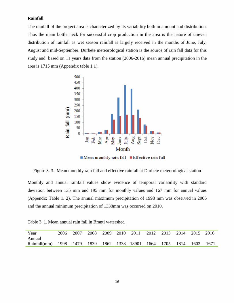
Rainfall
The rainfall of the project area is characterized by its variability both in amount and distribution.
Thus the main bottle neck for successful crop production in the area is the nature of uneven
distribution of rainfall as wet season rainfall is largely received in the months of June, July,
August and mid-September. Durbete meteorological station is the source of rain fall data for this
study and based on 11 years data from the station (2006-2016) mean annual precipitation in the
area is 1715 mm (Appendix table 1.1).
Figure 3. 3. Mean monthly rain fall and effective rainfall at Durbete meteorological station
Monthly and annual rainfall values show evidence of temporal variability with standard
deviation between 135 mm and 195 mm for monthly values and 167 mm for annual values
(Appendix Table 1. 2). The annual maximum precipitation of 1998 mm was observed in 2006
and the annual minimum precipitation of 1338mm was occurred on 2010.
Table 3. 1. Mean annual rain fall in Branti watershed
Year 2006 2007 2008 2009 2010 2011 2012 2013 2014 2015 2016
Annual
Rainfall(mm) 1998 1479 1839 1862 1338 18901 1664 1705 1814 1602 1671
17
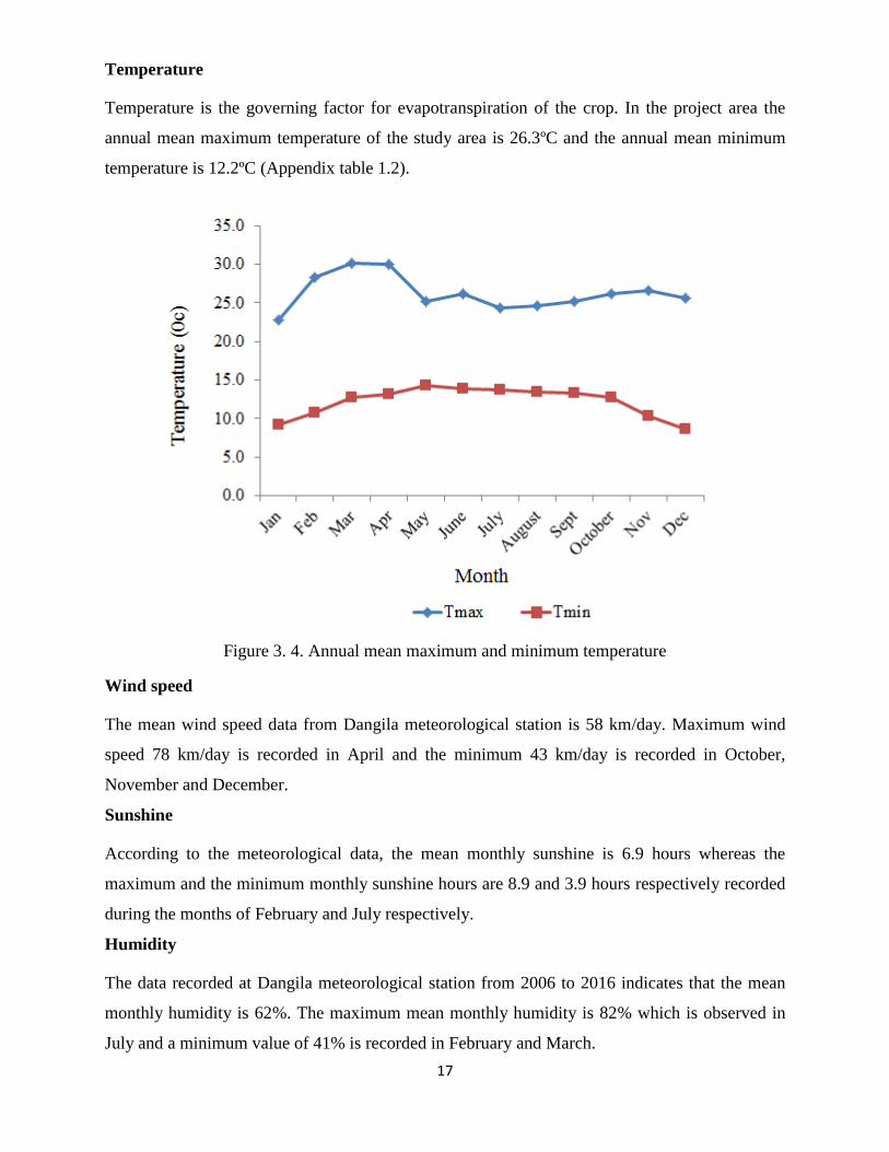
Temperature
Temperature is the governing factor for evapotranspiration of the crop. In the project area the
annual mean maximum temperature of the study area is 26.3ºC and the annual mean minimum
temperature is 12.2ºC (Appendix table 1.2).
Figure 3. 4. Annual mean maximum and minimum temperature
Wind speed
The mean wind speed data from Dangila meteorological station is 58 km/day. Maximum wind
speed 78 km/day is recorded in April and the minimum 43 km/day is recorded in October,
November and December.
Sunshine
According to the meteorological data, the mean monthly sunshine is 6.9 hours whereas the
maximum and the minimum monthly sunshine hours are 8.9 and 3.9 hours respectively recorded
during the months of February and July respectively.
Humidity
The data recorded at Dangila meteorological station from 2006 to 2016 indicates that the mean
monthly humidity is 62%. The maximum mean monthly humidity is 82% which is observed in
July and a minimum value of 41% is recorded in February and March.
18
3.1.3. Soil and topography
Topography is an important factor for the planning of any irrigation project as it influences
method of irrigation, drainage, erosion, mechanization, and cost of land development, labor
requirement and choice of crops. The topographic feature of the irrigation scheme has an
elevation (head work site) is about 1956 m.a.s.l. The slope gradient also ranges from flat (0.13%)
to gently sloping (≈5%). Hence, it has identified to be suitable for surface irrigation.
Nevertheless, catchments area above the irrigation scheme is not vegetated and soil erosion
during rainy season is a major problem causing canal sedimentation. There was not any soil
conservation structures constructed in the fields which contribute in reducing erosion in the field
during rain season. It requires soil and water conservation measures or structures.
Soil properties of a given catchment can be affecting physical and chemical characteristic of
plant growth, run of coefficient and irrigation efficiency. From the laboratory result (Table 4.1)
the dominant soil type of the command area is clay soil.
3.1.4. Description of Branti small-scale irrigation scheme
Branti small-scale irrigation scheme was constructed in 2010 G.C for satisfying the demands of
the farmers located within the Ahuri Keltafa kebele. Prior to the construction of the diversion
weir, farmers in the area had been practicing irrigation by diverting the Branti river using local
materials. The construction of the new diversion weir was done by Amhara Water Works
construction Enterprise and gave a service for 8 years operational period. The irrigation scheme
was originally designed to irrigate 68ha of land but the scheme currently irrigates 35ha.
The command area falls under moist Woina Dega (sub-moist cool) agro-ecological zone with an
average annual rainfall of 1715mm. As the source of water for the scheme is Branti river and
based on Cropwat estimation, required amount of water per ha (water duty) was estimated to be
1.65 l/s/ha and the capacity of intake gate was 112 l/s.
At present, the weir is functional but it needs major and minor maintenance for division box,
gates, main canal and secondary canals which are silted-up. It irrigates the land to the right side
of the river while for operation and management purpose the area was categorized into 7 water
user groups. The diversion weir has a crest of 38 meter length and 1.2 meter top width. The weir
height up to the crest level is estimated to be 3 meter and it has one sluice gate and one intake
gate.
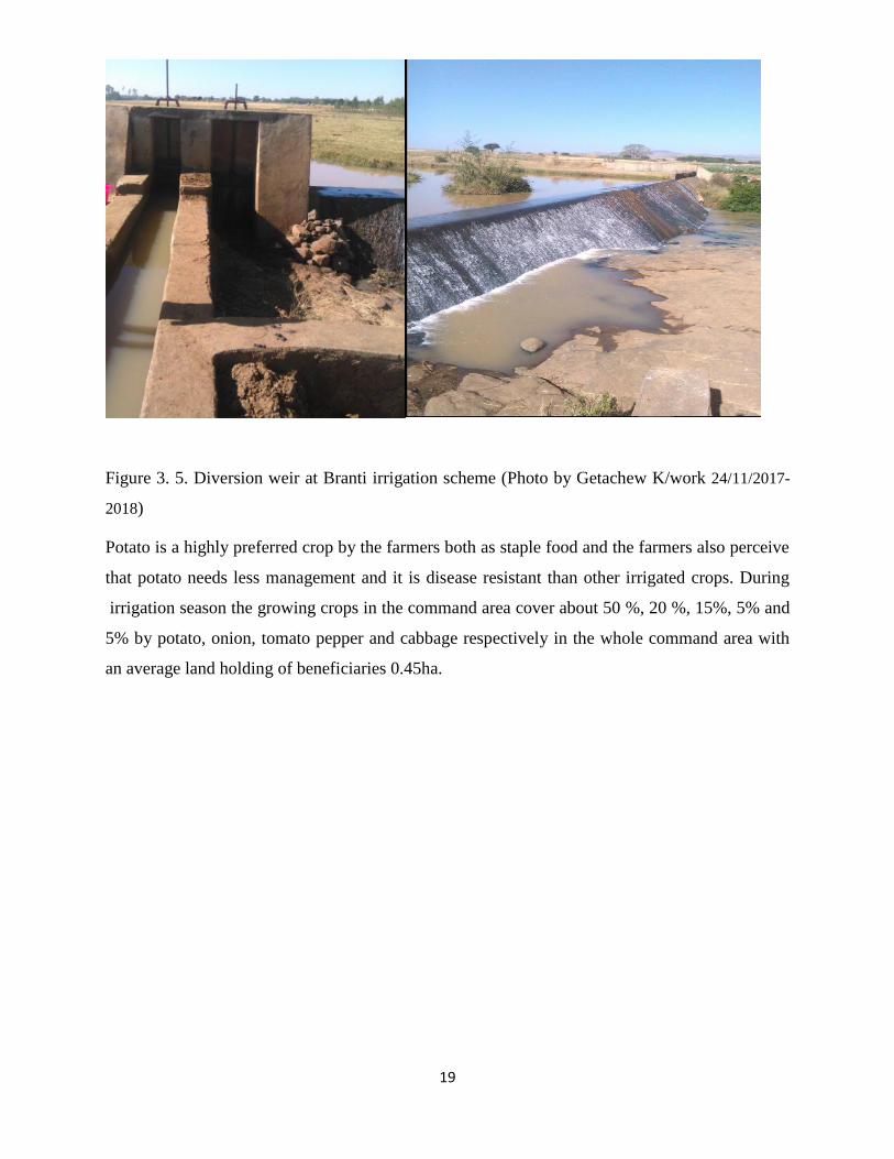
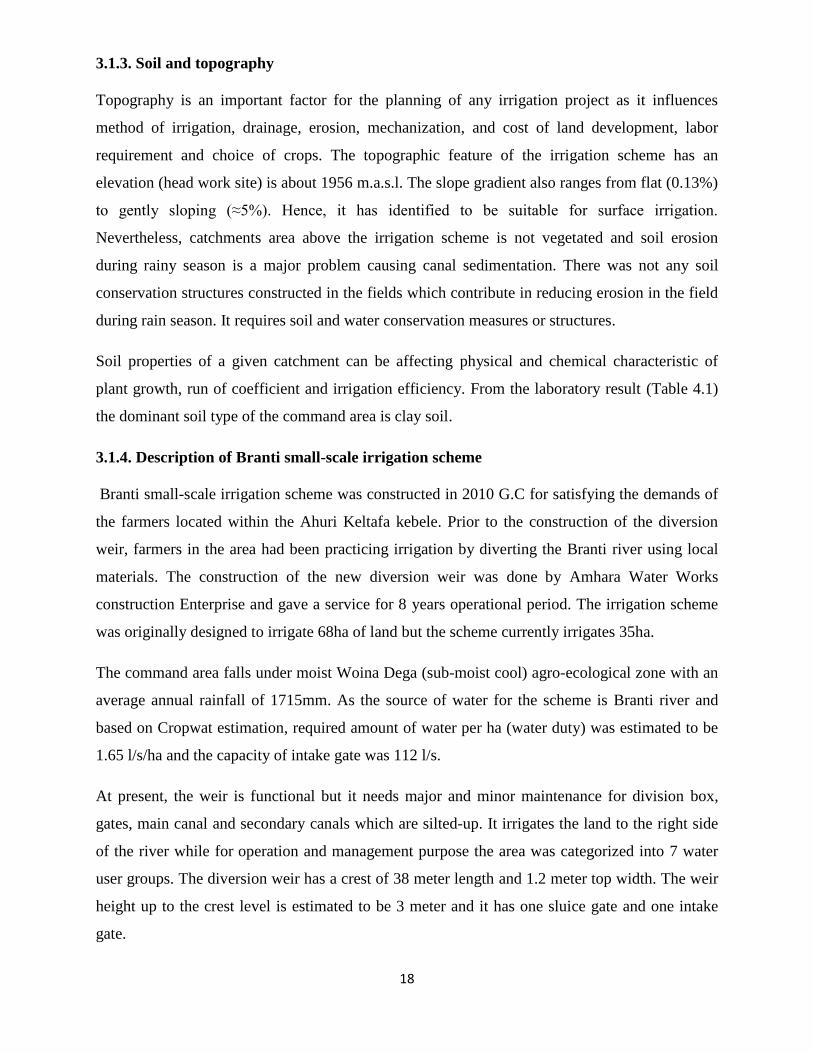
19
Figure 3. 5. Diversion weir at Branti irrigation scheme (Photo by Getachew K/work 24/11/2017-
2018)
Potato is a highly preferred crop by the farmers both as staple food and the farmers also perceive
that potato needs less management and it is disease resistant than other irrigated crops. During
irrigation season the growing crops in the command area cover about 50 %, 20 %, 15%, 5% and
5% by potato, onion, tomato pepper and cabbage respectively in the whole command area with
an average land holding of beneficiaries 0.45ha.
20
3.2. Methodology
3.2.1. Data Collection and analysis
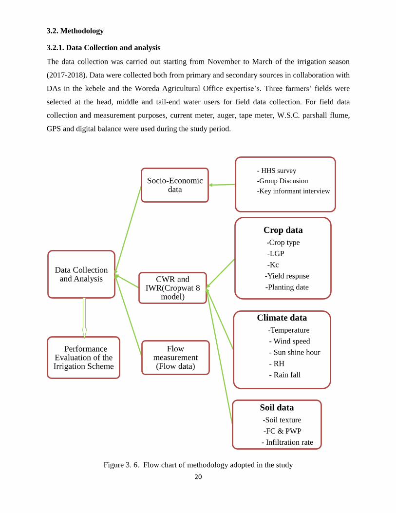
The data collection was carried out starting from November to March of the irrigation season
(2017-2018). Data were collected both from primary and secondary sources in collaboration with
DAs in the kebele and the Woreda Agricultural Office expertise’s. Three farmers’ fields were
selected at the head, middle and tail-end water users for field data collection. For field data
collection and measurement purposes, current meter, auger, tape meter, W.S.C. parshall flume,
GPS and digital balance were used during the study period.
Figure 3. 6. Flow chart of methodology adopted in the study
Data Collection and Analysis
Socio-Economic data
- HHS survey
-Group Discusion
-Key informant interview
CWR and IWR(Cropwat 8
model)
Crop data
-Crop type
-LGP
-Kc
-Yield respnse
-Planting date
Climate data
-Temperature
- Wind speed
- Sun shine hour
- RH
- Rain fall
Soil data
-Soil texture
-FC & PWP
- Infiltration rate
Flow measurement (Flow data)
Performance Evaluation of the Irrigation Scheme
21
3.2.1.1. Primary data collection
Frequent field observations were made to observe and investigate the method of water
applications made by the farmers. Measurements were made at farmer’s field in the head, middle
and tail water users to evaluate irrigation water applied to the field, soil moisture content before
and after irrigation events and observations have been made how farmers control and manage
irrigation water during application/irrigation events.
In order to evaluate the farmers’ perception about scheme performance and institutional
aspects, a sample size of 42 households were chosen out of total households. Stratification of
the scheme was based on location relative to the canals as head, middle and tail end users. A
sampling frame was obtained from most commonly available membership list. From this list
random sampling were used to select respondents from the total households.
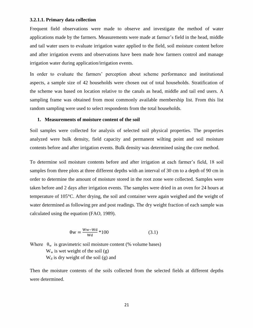
1. Measurements of moisture content of the soil
Soil samples were collected for analysis of selected soil physical properties. The properties
analyzed were bulk density, field capacity and permanent wilting point and soil moisture
contents before and after irrigation events. Bulk density was determined using the core method.
To determine soil moisture contents before and after irrigation at each farmer’s field, 18 soil
samples from three plots at three different depths with an interval of 30 cm to a depth of 90 cm in
order to determine the amount of moisture stored in the root zone were collected. Samples were
taken before and 2 days after irrigation events. The samples were dried in an oven for 24 hours at
temperature of 105°C. After drying, the soil and container were again weighed and the weight of
water determined as following pre and post readings. The dry weight fraction of each sample was
calculated using the equation (FAO, 1989).
*100 (3.1)
Where θw is gravimetric soil moisture content (% volume bases)
Ww is wet weight of the soil (g)
Wd is dry weight of the soil (g) and
Then the moisture contents of the soils collected from the selected fields at different depths
were determined.

22
To convert the dry weight soil moisture fraction into volumetric moisture content θ, the dry
weight fraction (θw) was multiplied by its respective bulk density ( ρb ) and divided by the
specific weight of water (ρ w) as follows:
(3.2)
2. Determination of soil texture, bulk density, field capacity and wilting point
Soil samples were taken to analysis the soil texture, bulk density and field capacity and wilting
point. The sampling points for the analysis of each parameter were distributed systematically
over the scheme so that most parts of the fields are represented.
To determine soil texture, 9 samples of disturbed soil samples were collected from different
locations in the field and determined in the laboratory using mechanical sieve analysis and
textural triangle. Bulk density of the study area was determined using 9 undisturbed soil samples
collected from three pits at interval of 30 cm starting from surface to a depth of 90 cm with core
samplers with volume of 98.125 cm3. The samples were placed in an oven and dried at 105°C for
24 hours. After drying, the soil and container were again weighed. Then dry weight of the soil
was divided by the sample volume to determine the dry bulk density.
Moisture contents at field capacity and wilting point were determined using 18 disturbed soil
samples collected from three sampling points at interval of 30 cm. Soil samples were soaked in
water for one day and a pressure of 1/3 and 15 bars were exerted in the laboratory using pressure
plate apparatus until no further change in soil moisture content was observed for the
determination of field capacity and permanent wilting point at Adet Research Center soil
laboratory (Table 4. 2).
3. Soil water availability
Soil water availability refers to the capacity of a soil to retain water available to plants. After
heavy rainfall or irrigation, the soil will drain until it reaches to field capacity. Field capacity
is the amount of water that a well-drained soil should hold against gravitational forces or the
amount of water remaining when downward drainage has markedly decreased.
The total available water in the root zone was taken as the difference between the water
content at field capacity and wilting point multiplied by Zr and 1000 as shown below (Allen et
al, 1998):-

23
θFc - θpwp) Zr (3.3)
Where: TAW = Total Available Water in the root zone [mm]
θFC = Water content at Field Capacity [m3 m-3]
θWP = Water content at Wilting Point [m3 m-3]
Zr = Rooting depth [m]
TAW is the amount of water that a crop can extract from its root zone and its magnitude
depends on the type of soil and the rooting depth. The fraction of TAW that a crop can extract
from the root zone without suffering water stress is the readily available soil water:
(3.4)
Where: RAW=the readily available soil water in the root zone [mm]
P=average fraction of total available soil water (TAW) that can be depleted
from the root zone before moisture stress (reduction in ET) occurs [0-1]
After determining of the readily available water, irrigation interval of the crops can be calculated
as follow as:-
(3.5)
If there are plants growing on the soil, the moisture level continues to drop until it reaches the
permanent wilting point (PWP). Soil moisture content near the wilting point is not readily
available to the plant. Hence the term readily available moisture has been used to refer to
that portion of the available moisture that is most easily extracted by the plants approximately
75% of the available moisture. After that, the plants cannot absorb water from the soil quickly
enough to replace water lost by transpiration (ICE, 1983).
4. Water channel flow rate measurement
Flow rate measurement is a relevant data for irrigation scheme performance evaluation activities
like computation of conveyance efficiency and losses. There are different methods to measure
the flow of water in canals. For this study current meter were used to measure water flow rate.
Flow measurements of the conveyance efficiency have been taken starting from intake to point
of main and secondary canals through using current meter. Measurement was taken at full supply
of the canals and in selecting the canal segment to measure losses; the following conditions were
24
taken into consideration (Australian National Committee on Irrigation and Drainage (ANCID,
2003)
a) The flow should be at normal operating condition of the canal
b) There should be no change in water level during measurement
c) There should be no water flow into canal or outside the canal
d) There should be nothing to prevent the flow and
e) Length of segment should be sufficient for measurement of conveyance losses.
Technique applied to determine losses was inflow-outflow discharge measurement at the canal
cross-section. For loss measurement canal length between two points, water depth and wetted
width was measured using tape meter. Discharge of the canal was calculated using velocity-area
method.
The velocity of flow at the selected cross-section was determined using counting number
of revolutions within 30 second (given value of the current meter used as stop-watch).
USBR (2001) classifies different methods of determining average flow velocities. Two point
method and Six-tenths depth methods are some of the listed methods to fix the propeller in order
to measure the depth. The two-point method involves of measuring the velocity at 0.2 and at 0.8
of the depth from the water surface and using the average of the two measurements.
In this study the six-tenths depth method consists of measuring the velocity at 0.6 of the depth
from the water surface is used. Water depth of the study canal was below 0.6 meter which is
shallow, so, the number of revolutions of this study was measured by fixing the current meter
propeller at 60% of the water depth from the water surface.
After calculating number of propeller rotation per second (n), then velocity of flow (cm/sec)
were calculated using equation (3.8). Finally the discharge was calculated using equation (3.6)
(3.6)
Where: Q=discharge rate [m3/sec]
A=canal cross-section [m2]
V=mean velocity of flow of water [m/s].
The area is determined using Equations
25
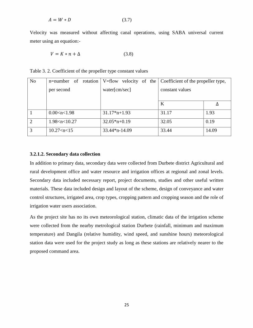
(3.7)
Velocity was measured without affecting canal operations, using SABA universal current
meter using an equation:-
(3.8)
Table 3. 2. Coefficient of the propeller type constant values
No n=number of rotation
per second
V=flow velocity of the
water[cm/sec]
Coefficient of the propeller type,
constant values
K
1 0.00<n<1.98 31.17*n+1.93 31.17 1.93
2 1.98<n<10.27 32.05*n+0.19 32.05 0.19
3 10.27<n<15 33.44*n-14.09 33.44 14.09
3.2.1.2. Secondary data collection
In addition to primary data, secondary data were collected from Durbete district Agricultural and
rural development office and water resource and irrigation offices at regional and zonal levels.
Secondary data included necessary report, project documents, studies and other useful written
materials. These data included design and layout of the scheme, design of conveyance and water
control structures, irrigated area, crop types, cropping pattern and cropping season and the role of
irrigation water users association.
As the project site has no its own meteorological station, climatic data of the irrigation scheme
were collected from the nearby metrological station Durbete (rainfall, minimum and maximum
temperature) and Dangila (relative humidity, wind speed, and sunshine hours) meteorological
station data were used for the project study as long as these stations are relatively nearer to the
proposed command area.
26
3.2.2. Determination of the Amount of Water Applied to the Fields
To determine the amount of water applied by farmers to the fields, a W.S.C. flume was installed
at the entrance of each field to measure the depth of water applied to the field. The measured
water depth was changed to its respective discharge by direct reading from calibration curve of
water level Vs Discharge graph (Appendix Figure 2.2).
During the determination of the amount of water applied to the field, the average water depth
of irrigation water passing through the flume to the field and respective time were recorded
with the size of the fields being irrigated. The total volume of water applied to the field was
obtained by multiplying the discharge rate with the inflow time. Then depth of water applied to
the field was obtained by dividing the total volume of water applied to the area being irrigated.
3.2.3. To assess water scarcity and irrigation water management of the irrigation scheme
3.2.3.1. Determination of crop water and irrigation water requirement
CROPWAT 8.0 computer program was used to estimate the total crop and irrigation water
requirements of major crops grown in the irrigation scheme. FAO (1992) Penman-Monteith
method was selected to calculate the reference crop evaporation (ETo) and the model needs
climatic, crop and soil data for the determination of crop and irrigation water requirements. To
determine ETo values the model requires climatic data of mean monthly minimum and
maximum temperature (0c), relative humidity (%), wind speed (km/day) and sunshine hours (hr).
The amount of water required to compensate the evapo-transpiration loss from the cropped field
is defined as crop water requirement. Crop water requirement refers to the amount of water that
needs to be supplied, while crop evapo-transpiration refers to the amount of water that is lost
through evapo-transpiration. So the program estimates (ETc) based on equation:-
(3.9)
Where: ETc=Crop evapo-transpiration
ETo=Reference crop evaporation
Kc= crop coefficients, varies with a crop growing stages.
The value of Kc of each major crops were taken from FAO I & D 24 (1992) and FAO 56 (1998)
papers. The determination of irrigation requirement was made after estimation of effective
rainfall by USDA Soil Conservation Service Method (Clarke et al., 1998).
27
Irrigation is required when rainfall is insufficient to compensate for the water lost by evapo-
transpiration. The primary objective of irrigation is to apply water at the right period and in the right
amount. By calculating the soil water balance/budget of the root zone on a daily basis, timing and the
depth of future irrigations can be planned. In order to compute the irrigation water requirement,
CROPWAT 8.0 computes a daily water balance of the root zone computed as:
(3.10)
Where: IWR=Irrigation water requirement
ETc=Crop evapo-transpiration
Peff =Effective rainfall
3.2.3.2.Irrigation scheduling
For determination of irrigation schedule of the irrigation scheme and to make comparison with
the current irrigation practices, moisture content at field capacity and permanent wilting point,
depletion fraction at each growing stage data were collected. Additionally farmer’s irrigation
practices were determined such as irrigation methods, irrigation frequency and interval of
irrigation and application depths. During the determination of the amount of water applied to
farmer’s field, the average water flow rate to the farm and respective time were recorded with the
size of the fields being irrigated.
The irrigation intervals at each growth stages of the main grown crops were determined
procedurally through equations [3.3], [3.4] and [3.5]. But in this research determination of
irrigation intervals and the depth of irrigation water applications at each growth stages was
determined by CROPWAT 8.0. Finally the irrigation schedules of main crops at the irrigation
scheme were determined.
3.2.4. Scheme Performance Evaluation
Performances of the schemes had been evaluated using performance indicators at farmer’s field.
The performance indicators computed were conveyance efficiency, application efficiency,
storage efficiency, runoff ratio, deep percolation fraction and overall scheme efficiency. For
computation purpose, a total of three farmer’s field plots were selected from irrigation scheme,
one from the head (H), one from the middle (M) and the other from the tail (T) end water users
of the irrigation scheme. The performance indicators for each scheme had been computed based
on field measured data as follow as:
28
3.2.4.1. Conveyance efficiency
Conveyance efficiency of the scheme was computed by taking discharges measurement at
different points. The measurements were taken at a point of diversion and at the initial and final
points of main and secondary canals using electro current meter. Water transport efficiency from
the source to the field is measured by conveyance efficiency. The first measurement of discharge
was conducted in the upper catchment of the main canal. In this canal section, the cross-section
of the channel was lined, uniform and rectangular in shape. Since the main canal had a
rectangular lined section for part of the system, the test site was ideal for flow measurement. The
width and depth of water flow in the canal was measured repeatedly and average was taken.
Conveyance efficiency can be calculated by dividing the second discharge by first discharge
using an equation:
*100 3.11
Where: Ec is conveyance efficiency (%),
Ws is amount of water diverted from the source (L/sec) and
Wf is amount of water at end point (L/sec).
The need of determining the conveyance efficiency is used to determine the losses in the canal
and the change of the ratio is an indicator for the need of maintenance. Water losses occur in
conveyance from the point of diversion until it reaches the farmer's fields which can be evaluated
by water conveyance efficiency. It was computed by:
(3.12)
Where: TL is the transmission loss of the canal in l/sec per100m
Q1 is inflow in [L/sec]
Q2 is out flow in [L/sec]
L is length of canal segment in 100 meter.
Losses of irrigation water occur during the transit from the head of a canal up to the farm
plot. In open canals, such losses take place primarily due to linkage and seepage. About 10
to 15% of the water admitted in to a canal can get lost in this way (Mazumder, 1983).
29
3.2.4.2. Application efficiency
When water is diverted into any water application system, part of the water infiltrates into the
soil for consumptive use by the crop while the rest is lost as deep percolation and runoff. The
efficiency terms determine these components and compare them with the volume of water
actually applied to the field. The term is an indication of the effectiveness of the system in
reducing losses during an irrigation event.
The application efficiency were computed as the ratio of moisture added to the soil profile due
to irrigation to the total water applied to the farm or the ratio of moisture retained due to
irrigation with total water added to the field. In this particular research soil samples had been
collected from different plots at different depths (0-30, 30-60 and 60-90 cm) and the amount of
water stored in the root zone were determined by gravimetric method.
The depth (Zr, mm) of moisture stored in the soil profile had been determined using the
following equation given by (Misra and Ahmed 1990)
∑ (3.13)
Where: Qf = moisture content of the ith
layer of soil after irrigation on oven dry weight basis [%]
Qi = moisture content of the ith
layer of soil before irrigation on oven dry weight basis [%]
ASi = Apparent specific gravity of the ith layer of soil [dimensionless]
Di = Depth of soil ith
layer [mm]
n = Number of layers in the root zone
To determine the amount of water applied by the farmers to the fields (D), a W.S.C.
flume were installed at the entrance of each field to measure the depth of water applied to the
field. Then measured water depth was changed to its respective discharge by direct reading from
calibration curve of water level Vs Discharge graph. During the determination of the amount of
water applied to the field, the average water depth of irrigation water passing through the flume
to the field and respective time were recorded with the size of the fields being irrigated.
Then the total volume of water applied to the field had been obtained by multiplying the
discharge rate with the inflow time. The depth of water applied to the field was obtained by
dividing the total volume of water applied to the area irrigated.
30
Finally, the application efficiency was computed as follows (Ramulu, 1998):
(3.14)
Where Ea is application efficiency (%), Zr is average depth of water applied to the root zone as
storage (mm) and D is average depth of water applied to the field (mm).It is used to determine
how much water used by the crop from total water supplied to the farm and it is an indication of
the effectiveness of the system in reducing losses during an irrigation event.
3.2.4.3. Storage efficiency
The storage efficiency is an index used to measure irrigation adequacy. It is the ratio of the
quantity of water stored in the root zone during irrigation event to that intended to be stored in
the root zone. The depth (Zr, mm) of moisture stored in the soil profile had been determined
using (equation 3.13). The depth of water that to be intended to be stored in the root zone was
computed by (equation 3.15) in the effective root zone based on the moisture content at field
capacity, permanent wilting point and bulk density of the soils of the selected irrigation fields.
The depth of irrigation water required by the crop was calculated (Misra and Ahmed 1990).
∑ (3.15)
After determining the storage and the required depths, the storage efficiency was calculated
using the following formula (Ramulu, 1998):
(3.16)
Where Er is storage efficiency (%), Zr is water stored in the root zone (mm), and Wn is water
desired to be stored in the root zone (mm).
3.2.4.4. Deep Percolation Fraction
The runoff ratio is normally considered zero where the farmers are using furrows whose tail ends
are closed, since for this study the furrows are closed end, runoff ratio is neglected. The loss of
water through drainage beyond the root zone is reflected only in the deep percolation ratio that
expresses the ratio between the percolated water beyond the root zone to the volume of water
applied to the field. Also the evaporation from the soil is marginal and can be neglected because
it is only a short period after irrigation. Therefore, the deep percolation ratio (%) can be
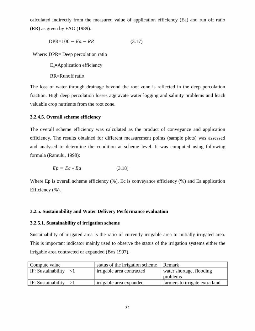
31
calculated indirectly from the measured value of application efficiency (Ea) and run off ratio
(RR) as given by FAO (1989).
DPR= (3.17)
Where: DPR= Deep percolation ratio
Ea=Application efficiency
RR=Runoff ratio
The loss of water through drainage beyond the root zone is reflected in the deep percolation
fraction. High deep percolation losses aggravate water logging and salinity problems and leach
valuable crop nutrients from the root zone.
3.2.4.5. Overall scheme efficiency
The overall scheme efficiency was calculated as the product of conveyance and application
efficiency. The results obtained for different measurement points (sample plots) was assessed
and analysed to determine the condition at scheme level. It was computed using following
formula (Ramulu, 1998):
(3.18)
Where Ep is overall scheme efficiency (%), Ec is conveyance efficiency (%) and Ea application
Efficiency (%).
3.2.5. Sustainability and Water Delivery Performance evaluation
3.2.5.1. Sustainability of irrigation scheme
Sustainability of irrigated area is the ratio of currently irrigable area to initially irrigated area.
This is important indicator mainly used to observe the status of the irrigation systems either the
irrigable area contracted or expanded (Bos 1997).
Compute value status of the irrigation scheme Remark
IF: Sustainability <1 irrigable area contracted water shortage, flooding
problems
IF: Sustainability >1 irrigable area expanded farmers to irrigate extra land
32
SIA =
(3.18)
Where: SIA=sustainability of the irrigation scheme
Currently irrigable area (ha)
Initially irrigated area= the designed irrigable area (ha)
3.2.5.2. Water Delivery Performance evaluation
Water delivery performance is the ratio of the amount of actual water delivered by the system to
the intended amount (Sanaee et al., 2000). This concept serves as an indicator of the performance
of an irrigation system to monitor productivity. According to (Bos et al., 1994), water delivery
performance is the simplest and the most important hydraulic performance indicator that
compares actual discharge to an intended or target discharge at any given location in the system.
Gross Irrigation Requirement
The gross irrigation requirement is the amount that must be delivered discharge. Gross irrigation
requirement is greater than net irrigation requirement by a factor which depends on the irrigation
efficiency:-
(3.20)
Where:-
• GIR = Gross irrigation requirement
• NIR = Net irrigation requirement
• E = Overall scheme efficiency
The value of designed (intended) discharge of water was taken from Cropwat software while
actually delivered of water will be measured directly from the canal with current meter.
(3.21)
Where: d is the delivery performance ratio (fraction)
Qa is actually delivered discharge of water (L/s) and
Qi Designed (intended) discharge of water to be delivered (L/s).

33
3.3. Institutional Aspect
To assess farmer’s perception about scheme performance, evaluations were made at the project
site by interviewing irrigation water beneficiary households with structured questionnaire. In
order to evaluate the farmers’ perception about scheme performance and institutional aspects a
sample size of 42 households was chosen out of 156 households. From these respondents 38
were male and 4 are female households.
Qualitative samples are usually small in size because if the data are properly analysed, there will
come a point where very little new evidence is obtained from each additional fieldwork unit,
(Ritchie et al., 2013). According to (Ritchie et al., 2013) as a very general rule of thumb,
qualitative samples for a single study involving individual interviews only often lie under 50. If
samples become much larger than 50 they start to become difficult to manage in terms of the
quality of data collection and analysis that can be achieved, it will also take much time and
budget.
The questioner data collected from randomly selected respondents had been analyzed using
Statistical Package for the Social Sciences version 20 (SPSS) program and discussed using
percentages. The questionnaires interview were conducted to identify key constraints of scheme
performance including planning and management, sustainability of the scheme, conflict and
conflict resolution mechanisms. All respondents were scheme beneficiaries which have been
selected from the head, middle and tail water users to provide information on irrigation problems
and on the performance of the scheme.
34
4. RESULTS AND DISCUSSION
4.1. Soil Characteristics
The soil textural class in the project area is dominantly clay (Table 4.1) for the selected plots in
the irrigation scheme indicating that soils in scheme are similar in texture at head, middle and
tail. The necessity of checking soil texture is an important parameter in performance evaluation
of irrigation scheme because the amount of irrigation water which can be given during irrigation
application influenced by the soil type. The soil type influences the maximum amount of water
which can be stored in the soil per metre depth. Sand can store only a little water or in other
words, sand has low available water content. On sandy soils it is necessary to irrigate frequently
with a small amount of water but clay soils have high available water content and thus on clayey
soils larger amounts can be given less frequently.
In addition to the soil type rooting depth of a crop also influences the maximum amount of water
which can be stored in the root zone. Thus, just after planting or sowing the crops need smaller
and more frequent water applications than when it is fully developed.
4.2. Soil data analysis results
Soil samples were collected at soil depth of 30, 60 and 90cm for analysis of soil physical
properties at Branti irrigation scheme. The properties analysed were particle size distribution,
bulk density and soil moisture contents at field capacity and permanent wilting point (Table 4.2).
4.2.1 .Particle size distribution (Texture)
The soil textural class of the irrigation scheme was determined based on the particle size
distribution through using USDA SCS Soil Textural Triangle method (Appendix
figure 2.1). Based on laboratory analysis as shown below, the soil textural class of the irrigation
scheme was found to be clay in the entire area.
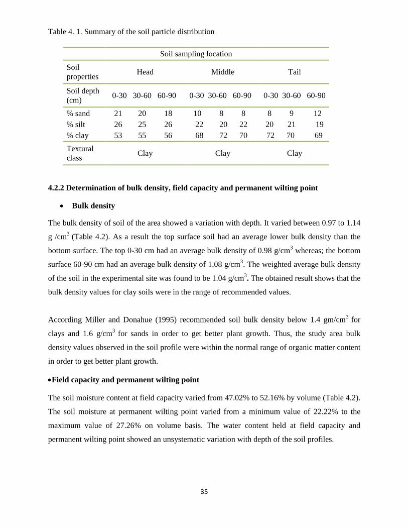
35
Table 4. 1. Summary of the soil particle distribution
Soil sampling location
Soil
properties Head Middle Tail
Soil depth
(cm) 0-30 30-60 60-90 0-30 30-60 60-90 0-30 30-60 60-90
% sand 21 20 18 10 8 8 8 9 12
% silt 26 25 26 22 20 22 20 21 19
% clay 53 55 56 68 72 70 72 70 69
Textural
class Clay Clay Clay
4.2.2 Determination of bulk density, field capacity and permanent wilting point
Bulk density
The bulk density of soil of the area showed a variation with depth. It varied between 0.97 to 1.14
g /cm3
(Table 4.2). As a result the top surface soil had an average lower bulk density than the
bottom surface. The top 0-30 cm had an average bulk density of 0.98 g/cm3 whereas; the bottom
surface 60-90 cm had an average bulk density of 1.08 g/cm3. The weighted average bulk density
of the soil in the experimental site was found to be 1.04 g/cm3. The obtained result shows that the
bulk density values for clay soils were in the range of recommended values.
According Miller and Donahue (1995) recommended soil bulk density below 1.4 gm/cm3
for
clays and 1.6 g/cm3
for sands in order to get better plant growth. Thus, the study area bulk
density values observed in the soil profile were within the normal range of organic matter content
in order to get better plant growth.
Field capacity and permanent wilting point
The soil moisture content at field capacity varied from 47.02% to 52.16% by volume (Table 4.2).
The soil moisture at permanent wilting point varied from a minimum value of 22.22% to the
maximum value of 27.26% on volume basis. The water content held at field capacity and
permanent wilting point showed an unsystematic variation with depth of the soil profiles.
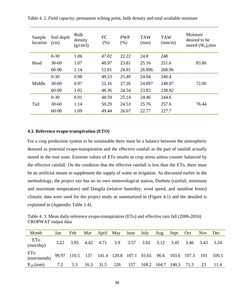
36
Table 4. 2. Field capacity, permanent wilting point, bulk density and total available moisture
Sample
location
Soil depth
(cm)
Bulk
density
(g/cm3)
FC
(%)
PWP
(%)
TAW
(mm)
TAW
(mm/m)
Moisture
desired to be
stored (Wn),mm
Head
0-30 1.06 47.02 22.22 24.8 248
83.86
30-60 1.07 48.97 23.81 25.16 251.6
60-90 1.14 51.81 24.91 26.896 268.96
Middle
0-30 0.98 49.53 25.49 24.04 240.4
72.00
30-60 0.97 52.16 27.26 24.897 248.97
60-90 1.02 48.36 24.54 23.82 238.82
Tail
0-30 0.91 48.59 25.14 24.46 244.6
76.44
30-60 1.14 50.29 24.53 25.76 257.6
60-90 1.09 49.44 26.67 22.77 227.7
4.3. Reference evapo-transpiration (ETO)
For a crop production system to be sustainable there must be a balance between the atmospheric
demand as potential evapo-transpiration and the effective rainfall as the part of rainfall actually
stored in the root zone. Extreme values of ETo results in crop stress unless counter balanced by
the effective rainfall. On the condition that the effective rainfall is less than the ETo, there must
be an artificial means to supplement the supply of water as irrigation. As discussed earlier in the
methodology, the project site has no its own meteorological station, Durbete (rainfall, minimum
and maximum temperature) and Dangila (relative humidity, wind speed, and sunshine hours)
climatic data were used for the project study as summarized in (Figure 4.1) and the detailed is
explained in (Appendix Table 1.4).
Table 4. 3. Mean daily reference evapo-transpiration (ETo) and effective rain fall (2006-2016)
CROPWAT output data
Month Jan Feb Mar April May June July Aug Sept Oct Nov Dec
ETo
(mm/day) 3.22 3.95 4.42 4.71 3.9 3.57 3.02 3.12 3.45 3.46 3.43 3.24
ETo
(mm/month) 99.97 110.5 137 141.4 120.8 107.1 93.65 96.6 103.6 107.3 103 100.5
Peff (mm) 7.2 3.3 16.3 31.5 126 157 168.2 164.7 140.3 71.3 23 11.4
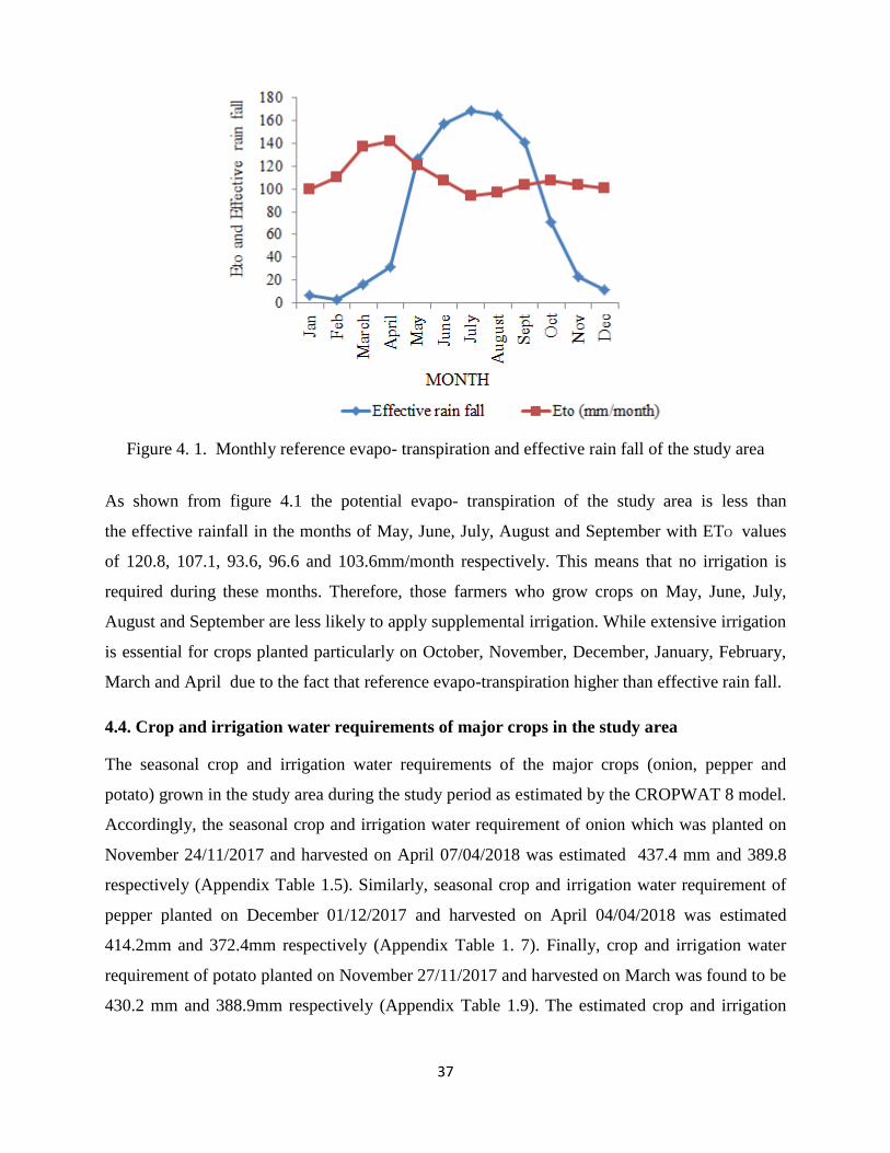
37
Figure 4. 1. Monthly reference evapo- transpiration and effective rain fall of the study area
As shown from figure 4.1 the potential evapo- transpiration of the study area is less than
the effective rainfall in the months of May, June, July, August and September with ETO values
of 120.8, 107.1, 93.6, 96.6 and 103.6mm/month respectively. This means that no irrigation is
required during these months. Therefore, those farmers who grow crops on May, June, July,
August and September are less likely to apply supplemental irrigation. While extensive irrigation
is essential for crops planted particularly on October, November, December, January, February,
March and April due to the fact that reference evapo-transpiration higher than effective rain fall.
4.4. Crop and irrigation water requirements of major crops in the study area
The seasonal crop and irrigation water requirements of the major crops (onion, pepper and
potato) grown in the study area during the study period as estimated by the CROPWAT 8 model.
Accordingly, the seasonal crop and irrigation water requirement of onion which was planted on
November 24/11/2017 and harvested on April 07/04/2018 was estimated 437.4 mm and 389.8
respectively (Appendix Table 1.5). Similarly, seasonal crop and irrigation water requirement of
pepper planted on December 01/12/2017 and harvested on April 04/04/2018 was estimated
414.2mm and 372.4mm respectively (Appendix Table 1. 7). Finally, crop and irrigation water
requirement of potato planted on November 27/11/2017 and harvested on March was found to be
430.2 mm and 388.9mm respectively (Appendix Table 1.9). The estimated crop and irrigation
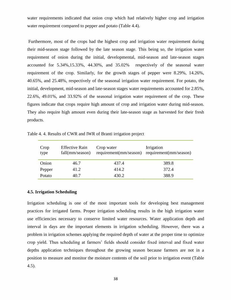
38
water requirements indicated that onion crop which had relatively higher crop and irrigation
water requirement compared to pepper and potato (Table 4.4).
Furthermore, most of the crops had the highest crop and irrigation water requirement during
their mid-season stage followed by the late season stage. This being so, the irrigation water
requirement of onion during the initial, developmental, mid-season and late-season stages
accounted for 5.34%,15.33%, 44.30%, and 35.02% respectively of the seasonal water
requirement of the crop. Similarly, for the growth stages of pepper were 8.29%, 14.26%,
40.65%, and 25.48%, respectively of the seasonal irrigation water requirement. For potato, the
initial, development, mid-season and late-season stages water requirements accounted for 2.85%,
22.6%, 49.01%, and 33.92% of the seasonal irrigation water requirement of the crop. These
figures indicate that crops require high amount of crop and irrigation water during mid-season.
They also require high amount even during their late-season stage as harvested for their fresh
products.
Table 4. 4. Results of CWR and IWR of Branti irrigation project
Crop
type
Effective Rain
fall(mm/season)
Crop water
requirement(mm/season)
Irrigation
requirement(mm/season)
Onion 46.7 437.4 389.8
Pepper 41.2 414.2 372.4
Potato 40.7 430.2 388.9
4.5. Irrigation Scheduling
Irrigation scheduling is one of the most important tools for developing best management
practices for irrigated farms. Proper irrigation scheduling results in the high irrigation water
use efficiencies necessary to conserve limited water resources. Water application depth and
interval in days are the important elements in irrigation scheduling. However, there was a
problem in irrigation schemes applying the required depth of water at the proper time to optimize
crop yield. Thus scheduling at farmers’ fields should consider fixed interval and fixed water
depths application techniques throughout the growing season because farmers are not in a
position to measure and monitor the moisture contents of the soil prior to irrigation event (Table
4.5).
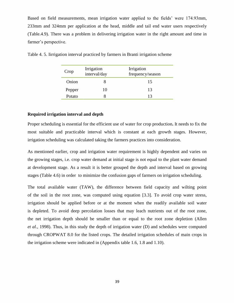
39
Based on field measurements, mean irrigation water applied to the fields’ were 174.93mm,
233mm and 324mm per application at the head, middle and tail end water users respectively
(Table.4.9). There was a problem in delivering irrigation water in the right amount and time in
farmer’s perspective.
Table 4. 5. Iirrigation interval practiced by farmers in Branti irrigation scheme
Required irrigation interval and depth
Proper scheduling is essential for the efficient use of water for crop production. It needs to fix the
most suitable and practicable interval which is constant at each growth stages. However,
irrigation scheduling was calculated taking the farmers practices into consideration.
As mentioned earlier, crop and irrigation water requirement is highly dependent and varies on
the growing stages, i.e. crop water demand at initial stage is not equal to the plant water demand
at development stage. As a result it is better grouped the depth and interval based on growing
stages (Table 4.6) in order to minimize the confusion gaps of farmers on irrigation scheduling.
The total available water (TAW), the difference between field capacity and wilting point
of the soil in the root zone, was computed using equation [3.3]. To avoid crop water stress,
irrigation should be applied before or at the moment when the readily available soil water
is depleted. To avoid deep percolation losses that may leach nutrients out of the root zone,
the net irrigation depth should be smaller than or equal to the root zone depletion (Allen
et al., 1998). Thus, in this study the depth of irrigation water (D) and schedules were computed
through CROPWAT 8.0 for the listed crops. The detailed irrigation schedules of main crops in
the irrigation scheme were indicated in (Appendix table 1.6, 1.8 and 1.10).
Crop Irrigation
interval/day
Irrigation
frequency/season
Onion 8 15
Pepper 10 13
Potato 8 13
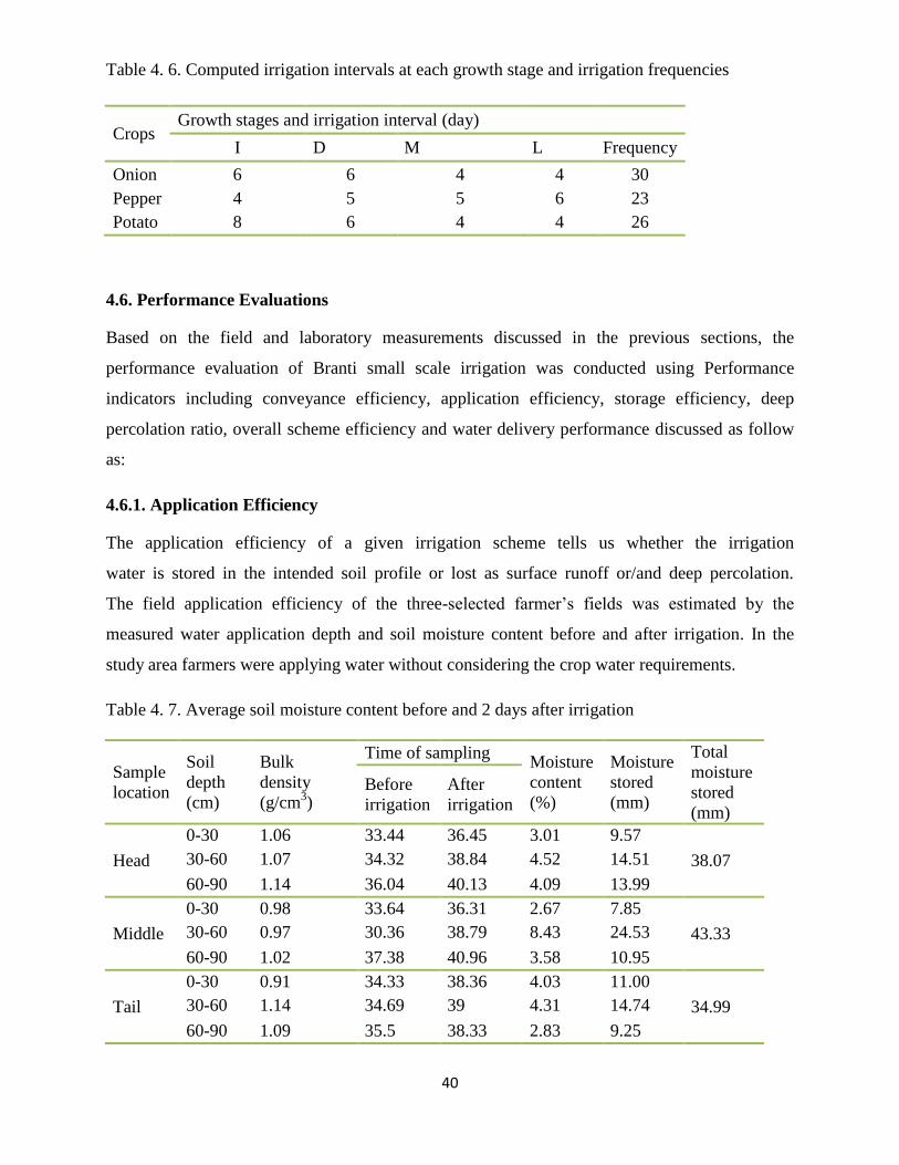
40
Table 4. 6. Computed irrigation intervals at each growth stage and irrigation frequencies
Crops Growth stages and irrigation interval (day)
I D M L Frequency
Onion 6 6 4 4 30
Pepper 4 5 5 6 23
Potato 8 6 4 4 26
4.6. Performance Evaluations
Based on the field and laboratory measurements discussed in the previous sections, the
performance evaluation of Branti small scale irrigation was conducted using Performance
indicators including conveyance efficiency, application efficiency, storage efficiency, deep
percolation ratio, overall scheme efficiency and water delivery performance discussed as follow
as:
4.6.1. Application Efficiency
The application efficiency of a given irrigation scheme tells us whether the irrigation
water is stored in the intended soil profile or lost as surface runoff or/and deep percolation.
The field application efficiency of the three-selected farmer’s fields was estimated by the
measured water application depth and soil moisture content before and after irrigation. In the
study area farmers were applying water without considering the crop water requirements.
Table 4. 7. Average soil moisture content before and 2 days after irrigation
Sample
location
Soil
depth
(cm)
Bulk
density
(g/cm3)
Time of sampling Moisture
content
(%)
Moisture
stored
(mm)
Total
moisture
stored
(mm)
Before
irrigation
After
irrigation
Head
0-30 1.06 33.44 36.45 3.01 9.57
38.07 30-60 1.07 34.32 38.84 4.52 14.51
60-90 1.14 36.04 40.13 4.09 13.99
Middle
0-30 0.98 33.64 36.31 2.67 7.85
43.33 30-60 0.97 30.36 38.79 8.43 24.53
60-90 1.02 37.38 40.96 3.58 10.95
Tail
0-30 0.91 34.33 38.36 4.03 11.00
34.99 30-60 1.14 34.69 39 4.31 14.74
60-90 1.09 35.5 38.33 2.83 9.25
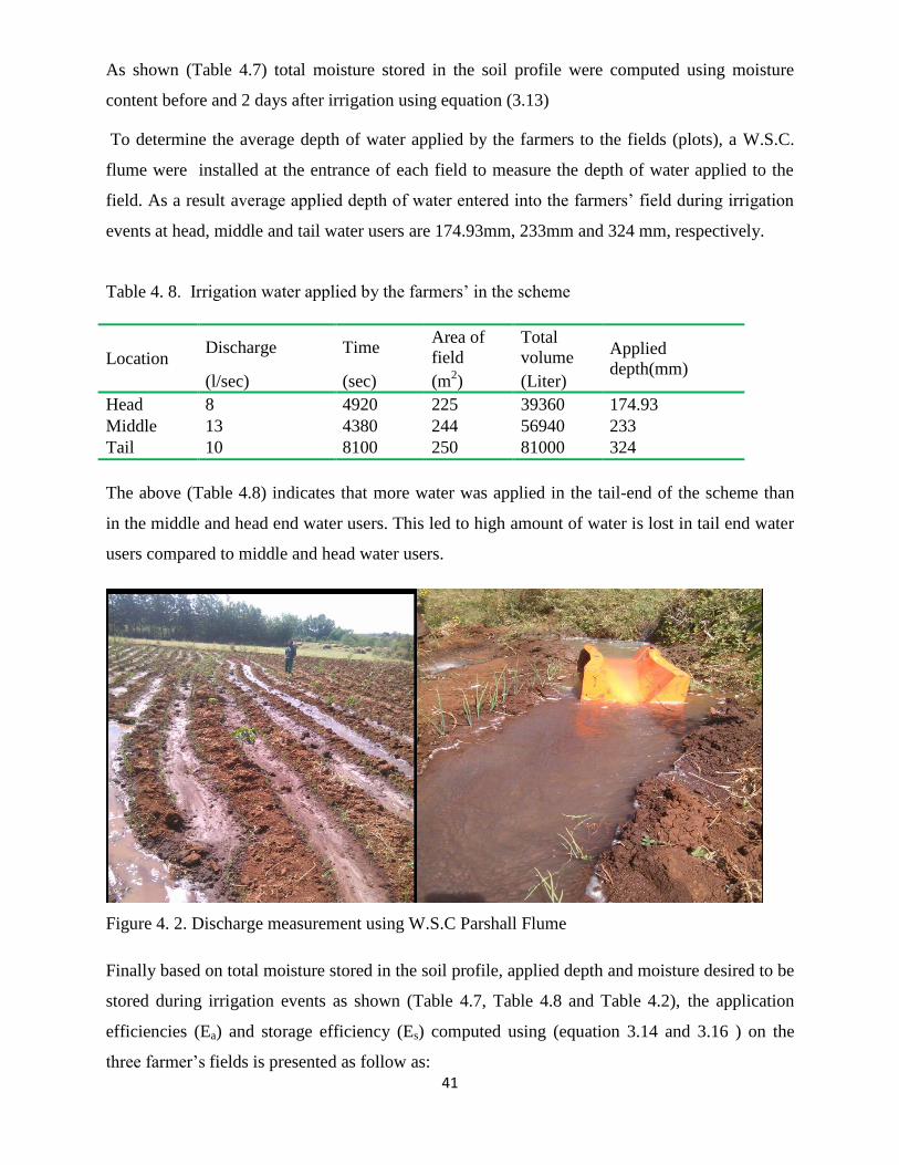
41
As shown (Table 4.7) total moisture stored in the soil profile were computed using moisture
content before and 2 days after irrigation using equation (3.13)
To determine the average depth of water applied by the farmers to the fields (plots), a W.S.C.
flume were installed at the entrance of each field to measure the depth of water applied to the
field. As a result average applied depth of water entered into the farmers’ field during irrigation
events at head, middle and tail water users are 174.93mm, 233mm and 324 mm, respectively.
Table 4. 8. Irrigation water applied by the farmers’ in the scheme
Location Discharge Time
Area of
field
Total
volume Applied
depth(mm) (l/sec) (sec) (m
2) (Liter)
Head 8 4920 225 39360 174.93
Middle 13 4380 244 56940 233
Tail 10 8100 250 81000 324
The above (Table 4.8) indicates that more water was applied in the tail-end of the scheme than
in the middle and head end water users. This led to high amount of water is lost in tail end water
users compared to middle and head water users.
Figure 4. 2. Discharge measurement using W.S.C Parshall Flume
Finally based on total moisture stored in the soil profile, applied depth and moisture desired to be
stored during irrigation events as shown (Table 4.7, Table 4.8 and Table 4.2), the application
efficiencies (Ea) and storage efficiency (Es) computed using (equation 3.14 and 3.16 ) on the
three farmer’s fields is presented as follow as:

42
Table 4. 9. Application and storage efficiencies of the selected fields
Location
Stored
depth
(mm)
Applied
depth
(mm)
Ea
(%)
Stored
depth
(mm)
Moisture
desired to
be stored
(mm)
Es (%)
Head 38.07 174.93 21.76 38.07 83.89 45.38
Middle 43.33 233 18.59 43.33 72.00 60.18
Tail 34.99 324 10.79 34.99 76.44 45.77
Average 38.79 243.97 17.05 38.79 77.44 50.44
As shown in the above (Table 4.9) the application efficiencies (Ea) computed on the three
farmers’ fields were in the range of 21.76%-10.79%, which was considered as inefficient and
indicating that the farmers were applying excess water to their fields. The reason behind low
application efficiency is much water was applied.
So that mean field application efficiency of the scheme was 17.05%. As to the recommended
value (60%) of FAO (1989), the application efficiencies of the three farmers’ fields were lower
than the recommended value which indicates that much of irrigation water applied to the field
was not stored in the soil.
Table 4. 10. Depth of water applied by farmers and irrigation requirement
Field
Depth applied in one irrigation event
(mm) Irrigation requirement (mm/season)
Head
174.93
389.8
Middle
233
372.4
Tail 324 388.9
As shown in (Table 4.10), depth of water applied during one irrigation event to the selected
farmers’ field located at the head, middle and tail-end equals to 174.93 mm, 233 mm and
324 mm respectively. However, the calculated irrigation water requirement using CROPWAT 8
in the head, middle and tail-end were 389.8 mm/season, 372.4 mm/season and 388.9 mm/season
respectively. This implies that the amount of water applied to the fields during one irrigation
event was too much. Therefore, this result indicates wastage of scarce resource in the irrigation
scheme.
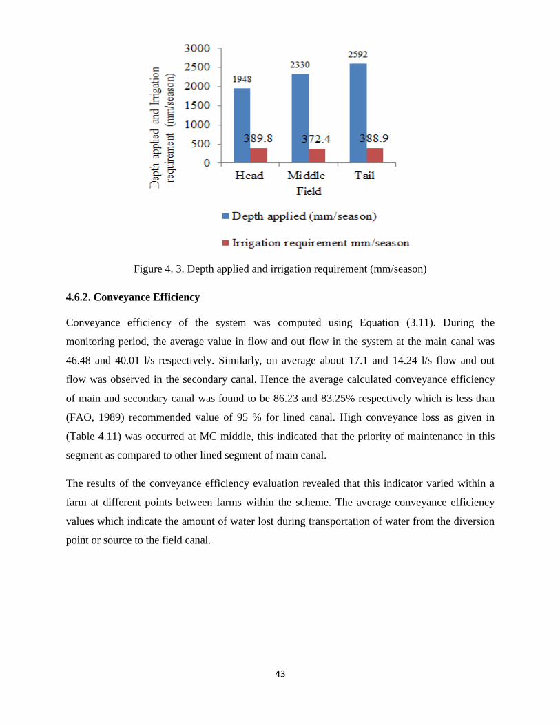
43
Figure 4. 3. Depth applied and irrigation requirement (mm/season)
4.6.2. Conveyance Efficiency
Conveyance efficiency of the system was computed using Equation (3.11). During the
monitoring period, the average value in flow and out flow in the system at the main canal was
46.48 and 40.01 l/s respectively. Similarly, on average about 17.1 and 14.24 l/s flow and out
flow was observed in the secondary canal. Hence the average calculated conveyance efficiency
of main and secondary canal was found to be 86.23 and 83.25% respectively which is less than
(FAO, 1989) recommended value of 95 % for lined canal. High conveyance loss as given in
(Table 4.11) was occurred at MC middle, this indicated that the priority of maintenance in this
segment as compared to other lined segment of main canal.
The results of the conveyance efficiency evaluation revealed that this indicator varied within a
farm at different points between farms within the scheme. The average conveyance efficiency
values which indicate the amount of water lost during transportation of water from the diversion
point or source to the field canal.

44
Table 4. 11. Conveyance efficiency of main and secondary canal
Canal
type System
Mean discharge
inflow(l/sec)
Mean discharge
out flow(l/sec)
Distance between
inflow_ out flow
points (m)
Ec (%)
Main
canal
MC Head 47.12 40.5 202 85.95
MC Middle 47.66 37.87 350 79.46
MC Tail 44.67 41.67 400 93.28
Secondary
canal
SC1Head to
tail 17.7 14.67 250 82.88
SC2 Head to
tail 16.5 13.8 300 83.63
The distance in the main canal from main intake to head, from head to middle and from
middle to tail-end was 202 m, 350 m and 400 m, respectively. Thus, the loss in discharge
per meter length in the main canal from main intake to head, from head to middle and from
middle to tail-end was 0.0066 l/s/m, 0.028 l/s/m and 0.0075 l/s/m, respectively using (equation
3.12). This implies that a significant amount of irrigation water was lost in the main canal
middle. The loss in the main canal is mainly related to leakage/ seepage losses, unauthorized
diversion of water by farmers into field ditches and overtopping of the water from the canal
(Figure 4.4).

45
(a) (b)
(c) (d)
Figure 4.4. (a) Discharge measurement using current meter (b) Illegal canal water abstraction
(c) Leakage/ seepage losses in main canal, (d) Overtopping of water
4.6.3. Storage efficiency
The storage efficiency is an index used to measure irrigation adequacy. It is the ratio of the
quantity of water stored in the root zone during irrigation event to that intended to be stored in
the root zone. It becomes important when water supplies are limited or when excessive time is
required to secure adequate penetration of water into the soil. Mean water storage efficiency (Es)
computed using (equation 3.16) indicate that the storage efficiency of these fields can be
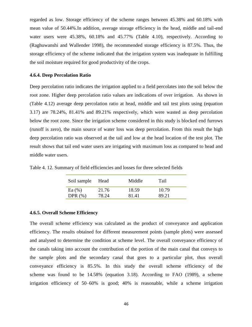
46
regarded as low. Storage efficiency of the scheme ranges between 45.38% and 60.18% with
mean value of 50.44%.In addition, average storage efficiency in the head, middle and tail-end
water users were 45.38%, 60.18% and 45.77% (Table 4.10), respectively. According to
(Raghuwanshi and Wallender 1998), the recommended storage efficiency is 87.5%. Thus, the
storage efficiency of the scheme indicated that the irrigation system was inadequate in fulfilling
the soil moisture required for good productivity of the crops.
4.6.4. Deep Percolation Ratio
Deep percolation ratio indicates the irrigation applied to a field percolates into the soil below the
root zone. Higher deep percolation ratio values are indications of over irrigation. As shown in
(Table 4.12) average deep percolation ratio at head, middle and tail test plots using (equation
3.17) are 78.24%, 81.41% and 89.21% respectively, which were wasted as deep percolation
below the root zone. Since the irrigation scheme considered in this study is blocked end furrows
(runoff is zero), the main source of water loss was deep percolation. From this result the high
deep percolation ratio was observed at the tail and low at the head location of the test plot. The
result shows that tail end water users are irrigating with maximum loss as compared to head and
middle water users.
Table 4. 12. Summary of field efficiencies and losses for three selected fields
Soil sample Head Middle Tail
Ea (%) 21.76 18.59 10.79
DPR (%) 78.24 81.41 89.21
4.6.5. Overall Scheme Efficiency
The overall scheme efficiency was calculated as the product of conveyance and application
efficiency. The results obtained for different measurement points (sample plots) were assessed
and analysed to determine the condition at scheme level. The overall conveyance efficiency of
the canals taking into account the contribution of the portion of the main canal that conveys to
the sample plots and the secondary canal that goes to a particular plot, thus overall
conveyance efficiency is 85.5%. In this study the overall scheme efficiency of the
scheme was found to be 14.58% (equation 3.18). According to FAO (1989), a scheme
irrigation efficiency of 50–60% is good; 40% is reasonable, while a scheme irrigation
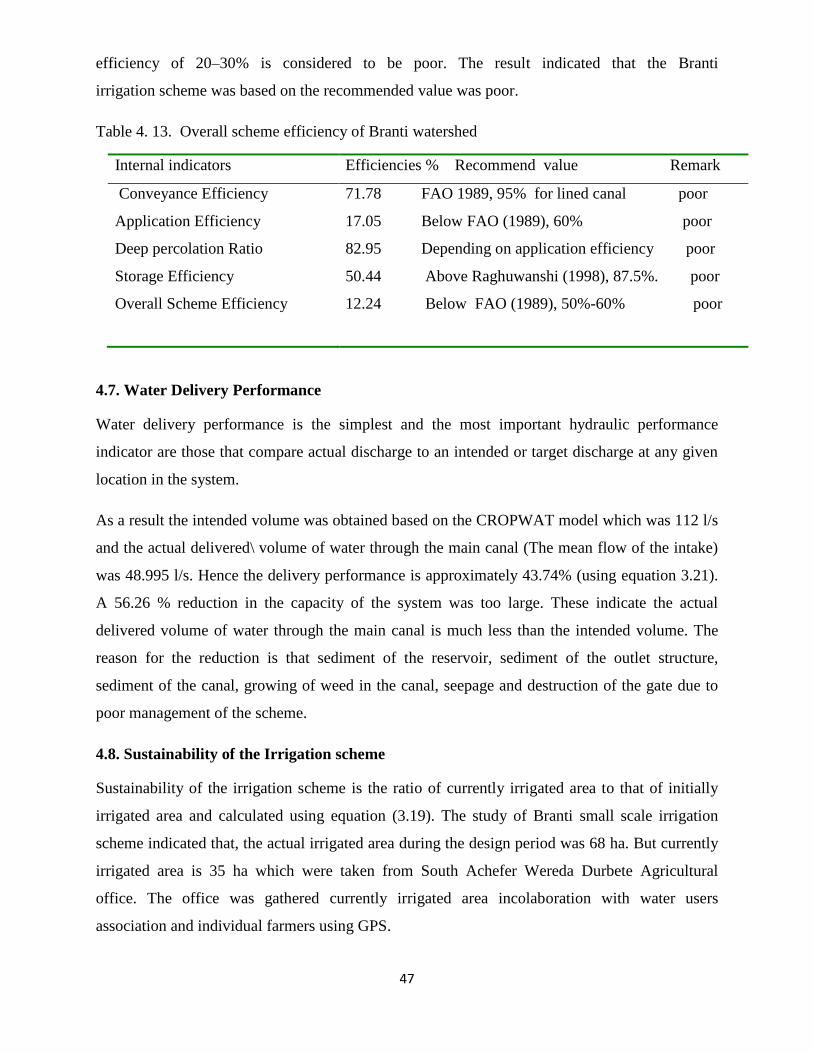
47
efficiency of 20–30% is considered to be poor. The result indicated that the Branti
irrigation scheme was based on the recommended value was poor.
Table 4. 13. Overall scheme efficiency of Branti watershed
Internal indicators Efficiencies % Recommend value Remark
Conveyance Efficiency 71.78 FAO 1989, 95% for lined canal poor
Application Efficiency 17.05 Below FAO (1989), 60% poor
Deep percolation Ratio 82.95 Depending on application efficiency poor
Storage Efficiency 50.44 Above Raghuwanshi (1998), 87.5%. poor
Overall Scheme Efficiency 12.24 Below FAO (1989), 50%-60% poor
4.7. Water Delivery Performance
Water delivery performance is the simplest and the most important hydraulic performance
indicator are those that compare actual discharge to an intended or target discharge at any given
location in the system.
As a result the intended volume was obtained based on the CROPWAT model which was 112 l/s
and the actual delivered\ volume of water through the main canal (The mean flow of the intake)
was 48.995 l/s. Hence the delivery performance is approximately 43.74% (using equation 3.21).
A 56.26 % reduction in the capacity of the system was too large. These indicate the actual
delivered volume of water through the main canal is much less than the intended volume. The
reason for the reduction is that sediment of the reservoir, sediment of the outlet structure,
sediment of the canal, growing of weed in the canal, seepage and destruction of the gate due to
poor management of the scheme.
4.8. Sustainability of the Irrigation scheme
Sustainability of the irrigation scheme is the ratio of currently irrigated area to that of initially
irrigated area and calculated using equation (3.19). The study of Branti small scale irrigation
scheme indicated that, the actual irrigated area during the design period was 68 ha. But currently
irrigated area is 35 ha which were taken from South Achefer Wereda Durbete Agricultural
office. The office was gathered currently irrigated area incolaboration with water users
association and individual farmers using GPS.
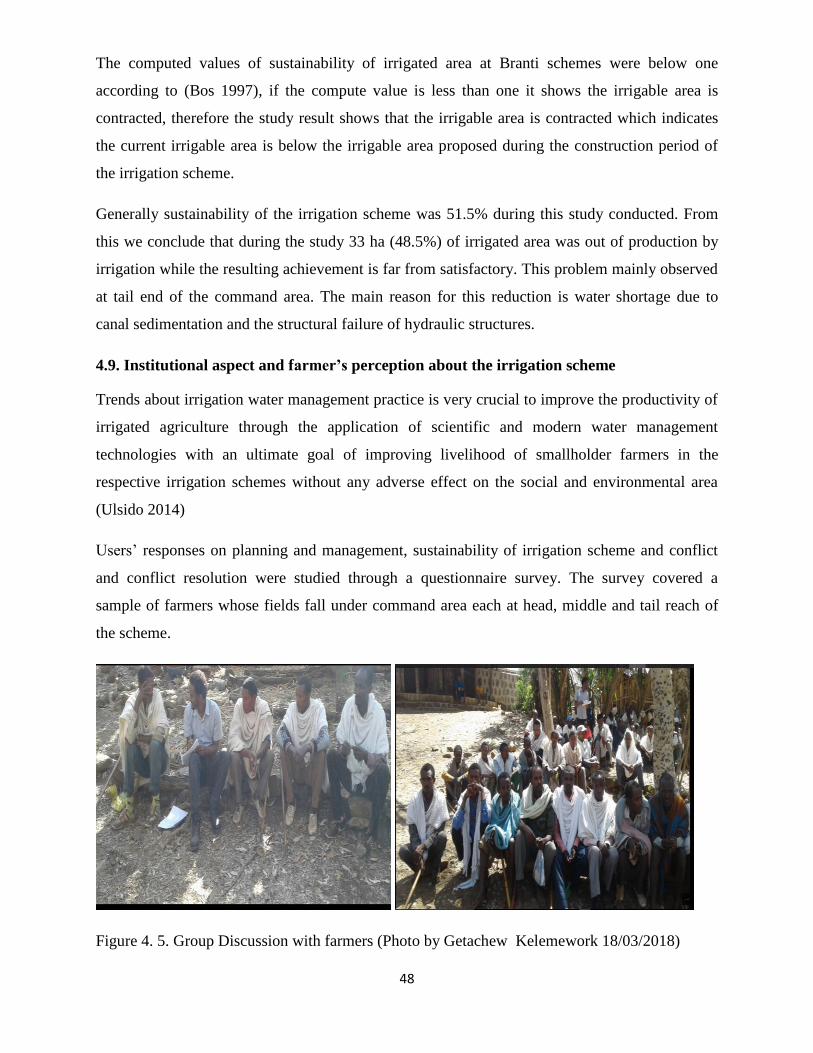
48
The computed values of sustainability of irrigated area at Branti schemes were below one
according to (Bos 1997), if the compute value is less than one it shows the irrigable area is
contracted, therefore the study result shows that the irrigable area is contracted which indicates
the current irrigable area is below the irrigable area proposed during the construction period of
the irrigation scheme.
Generally sustainability of the irrigation scheme was 51.5% during this study conducted. From
this we conclude that during the study 33 ha (48.5%) of irrigated area was out of production by
irrigation while the resulting achievement is far from satisfactory. This problem mainly observed
at tail end of the command area. The main reason for this reduction is water shortage due to
canal sedimentation and the structural failure of hydraulic structures.
4.9. Institutional aspect and farmer’s perception about the irrigation scheme
Trends about irrigation water management practice is very crucial to improve the productivity of
irrigated agriculture through the application of scientific and modern water management
technologies with an ultimate goal of improving livelihood of smallholder farmers in the
respective irrigation schemes without any adverse effect on the social and environmental area
(Ulsido 2014)
Users’ responses on planning and management, sustainability of irrigation scheme and conflict
and conflict resolution were studied through a questionnaire survey. The survey covered a
sample of farmers whose fields fall under command area each at head, middle and tail reach of
the scheme.
Figure 4. 5. Group Discussion with farmers (Photo by Getachew Kelemework 18/03/2018)
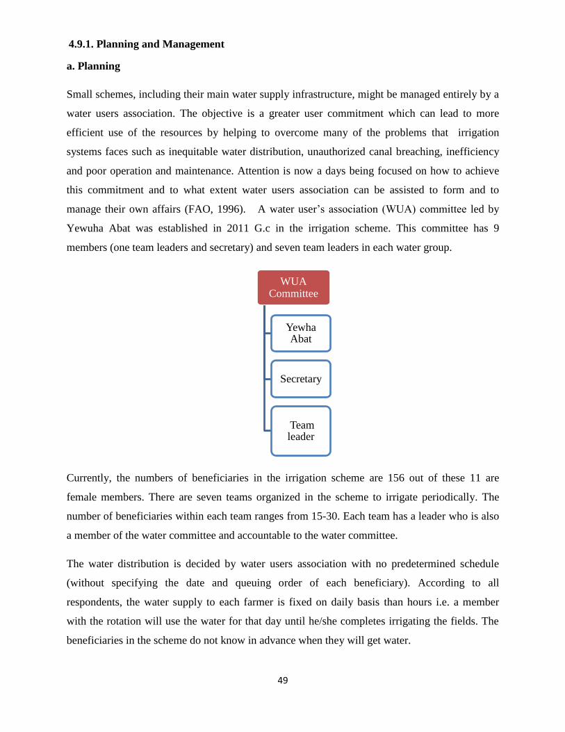
49
4.9.1. Planning and Management
a. Planning
Small schemes, including their main water supply infrastructure, might be managed entirely by a
water users association. The objective is a greater user commitment which can lead to more
efficient use of the resources by helping to overcome many of the problems that irrigation
systems faces such as inequitable water distribution, unauthorized canal breaching, inefficiency
and poor operation and maintenance. Attention is now a days being focused on how to achieve
this commitment and to what extent water users association can be assisted to form and to
manage their own affairs (FAO, 1996). A water user’s association (WUA) committee led by
Yewuha Abat was established in 2011 G.c in the irrigation scheme. This committee has 9
members (one team leaders and secretary) and seven team leaders in each water group.
Currently, the numbers of beneficiaries in the irrigation scheme are 156 out of these 11 are
female members. There are seven teams organized in the scheme to irrigate periodically. The
number of beneficiaries within each team ranges from 15-30. Each team has a leader who is also
a member of the water committee and accountable to the water committee.
The water distribution is decided by water users association with no predetermined schedule
(without specifying the date and queuing order of each beneficiary). According to all
respondents, the water supply to each farmer is fixed on daily basis than hours i.e. a member
with the rotation will use the water for that day until he/she completes irrigating the fields. The
beneficiaries in the scheme do not know in advance when they will get water.
WUA Committee
Yewha Abat
Secretary
Team leader
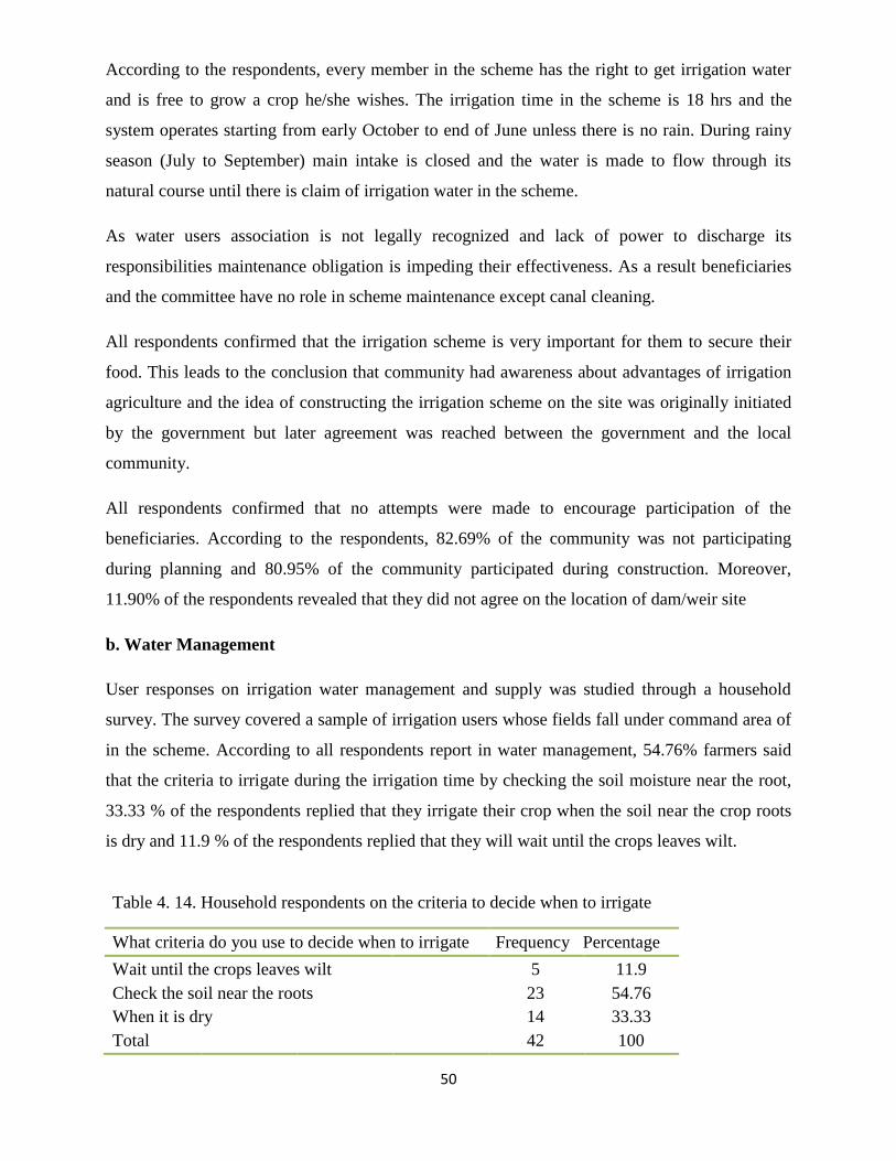
50
According to the respondents, every member in the scheme has the right to get irrigation water
and is free to grow a crop he/she wishes. The irrigation time in the scheme is 18 hrs and the
system operates starting from early October to end of June unless there is no rain. During rainy
season (July to September) main intake is closed and the water is made to flow through its
natural course until there is claim of irrigation water in the scheme.
As water users association is not legally recognized and lack of power to discharge its
responsibilities maintenance obligation is impeding their effectiveness. As a result beneficiaries
and the committee have no role in scheme maintenance except canal cleaning.
All respondents confirmed that the irrigation scheme is very important for them to secure their
food. This leads to the conclusion that community had awareness about advantages of irrigation
agriculture and the idea of constructing the irrigation scheme on the site was originally initiated
by the government but later agreement was reached between the government and the local
community.
All respondents confirmed that no attempts were made to encourage participation of the
beneficiaries. According to the respondents, 82.69% of the community was not participating
during planning and 80.95% of the community participated during construction. Moreover,
11.90% of the respondents revealed that they did not agree on the location of dam/weir site
b. Water Management
User responses on irrigation water management and supply was studied through a household
survey. The survey covered a sample of irrigation users whose fields fall under command area of
in the scheme. According to all respondents report in water management, 54.76% farmers said
that the criteria to irrigate during the irrigation time by checking the soil moisture near the root,
33.33 % of the respondents replied that they irrigate their crop when the soil near the crop roots
is dry and 11.9 % of the respondents replied that they will wait until the crops leaves wilt.
Table 4. 14. Household respondents on the criteria to decide when to irrigate
What criteria do you use to decide when to irrigate Frequency Percentage
Wait until the crops leaves wilt 5 11.9
Check the soil near the roots
23 54.76
When it is dry
14 33.33
Total 42 100
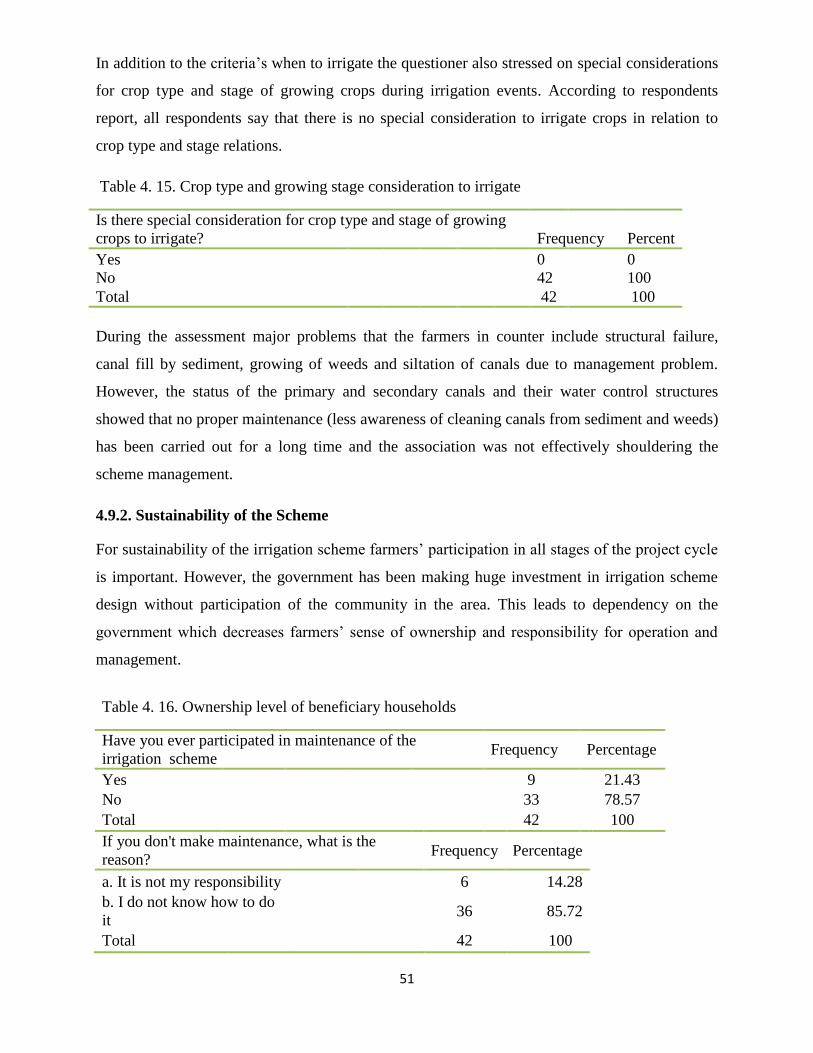
51
In addition to the criteria’s when to irrigate the questioner also stressed on special considerations
for crop type and stage of growing crops during irrigation events. According to respondents
report, all respondents say that there is no special consideration to irrigate crops in relation to
crop type and stage relations.
Table 4. 15. Crop type and growing stage consideration to irrigate
Is there special consideration for crop type and stage of growing
crops to irrigate? Frequency Percent
Yes
0
0
No
42
100
Total 42 100
During the assessment major problems that the farmers in counter include structural failure,
canal fill by sediment, growing of weeds and siltation of canals due to management problem.
However, the status of the primary and secondary canals and their water control structures
showed that no proper maintenance (less awareness of cleaning canals from sediment and weeds)
has been carried out for a long time and the association was not effectively shouldering the
scheme management.
4.9.2. Sustainability of the Scheme
For sustainability of the irrigation scheme farmers’ participation in all stages of the project cycle
is important. However, the government has been making huge investment in irrigation scheme
design without participation of the community in the area. This leads to dependency on the
government which decreases farmers’ sense of ownership and responsibility for operation and
management.
Table 4. 16. Ownership level of beneficiary households
Have you ever participated in maintenance of the
irrigation scheme Frequency Percentage
Yes
9 21.43
No
33 78.57
Total 42 100
If you don't make maintenance, what is the
reason? Frequency Percentage
a. It is not my responsibility
6 14.28
b. I do not know how to do
it
36 85.72
Total 42 100
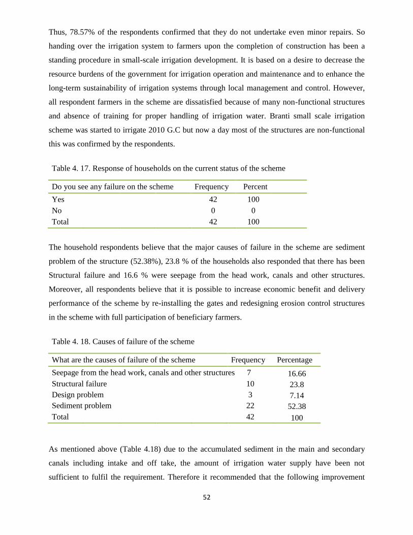
52
Thus, 78.57% of the respondents confirmed that they do not undertake even minor repairs. So
handing over the irrigation system to farmers upon the completion of construction has been a
standing procedure in small-scale irrigation development. It is based on a desire to decrease the
resource burdens of the government for irrigation operation and maintenance and to enhance the
long-term sustainability of irrigation systems through local management and control. However,
all respondent farmers in the scheme are dissatisfied because of many non-functional structures
and absence of training for proper handling of irrigation water. Branti small scale irrigation
scheme was started to irrigate 2010 G.C but now a day most of the structures are non-functional
this was confirmed by the respondents.
Table 4. 17. Response of households on the current status of the scheme
Do you see any failure on the scheme Frequency Percent
Yes
42 100
No
0 0
Total 42 100
The household respondents believe that the major causes of failure in the scheme are sediment
problem of the structure (52.38%), 23.8 % of the households also responded that there has been
Structural failure and 16.6 % were seepage from the head work, canals and other structures.
Moreover, all respondents believe that it is possible to increase economic benefit and delivery
performance of the scheme by re-installing the gates and redesigning erosion control structures
in the scheme with full participation of beneficiary farmers.
Table 4. 18. Causes of failure of the scheme
What are the causes of failure of the scheme Frequency Percentage
Seepage from the head work, canals and other structures 7 16.66
Structural failure
10 23.8
Design problem
3 7.14
Sediment problem
22 52.38
Total 42 100
As mentioned above (Table 4.18) due to the accumulated sediment in the main and secondary
canals including intake and off take, the amount of irrigation water supply have been not
sufficient to fulfil the requirement. Therefore it recommended that the following improvement
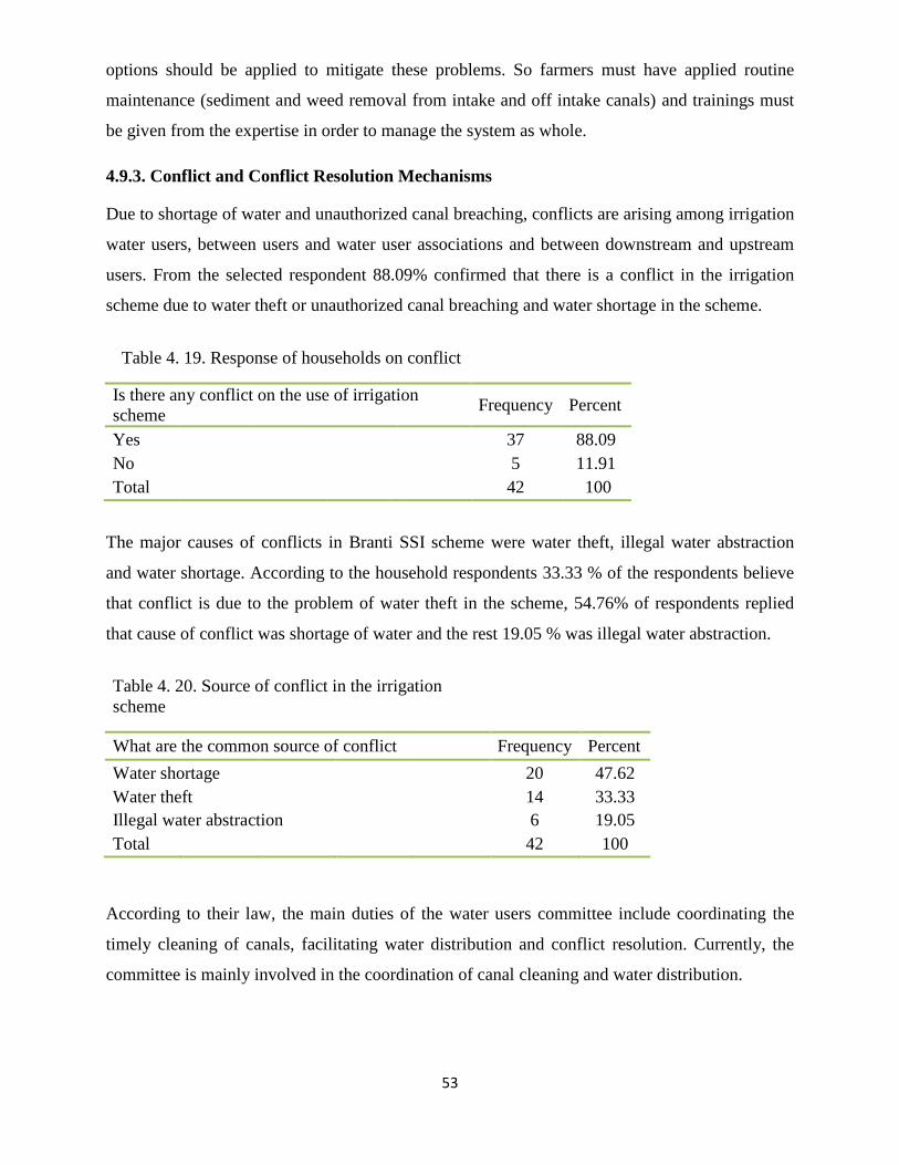
53
options should be applied to mitigate these problems. So farmers must have applied routine
maintenance (sediment and weed removal from intake and off intake canals) and trainings must
be given from the expertise in order to manage the system as whole.
4.9.3. Conflict and Conflict Resolution Mechanisms
Due to shortage of water and unauthorized canal breaching, conflicts are arising among irrigation
water users, between users and water user associations and between downstream and upstream
users. From the selected respondent 88.09% confirmed that there is a conflict in the irrigation
scheme due to water theft or unauthorized canal breaching and water shortage in the scheme.
Table 4. 19. Response of households on conflict
Is there any conflict on the use of irrigation
scheme Frequency Percent
Yes
37 88.09
No
5 11.91
Total 42 100
The major causes of conflicts in Branti SSI scheme were water theft, illegal water abstraction
and water shortage. According to the household respondents 33.33 % of the respondents believe
that conflict is due to the problem of water theft in the scheme, 54.76% of respondents replied
that cause of conflict was shortage of water and the rest 19.05 % was illegal water abstraction.
Table 4. 20. Source of conflict in the irrigation
scheme
What are the common source of conflict Frequency Percent
Water shortage
20 47.62
Water theft
14 33.33
Illegal water abstraction
6 19.05
Total 42 100
According to their law, the main duties of the water users committee include coordinating the
timely cleaning of canals, facilitating water distribution and conflict resolution. Currently, the
committee is mainly involved in the coordination of canal cleaning and water distribution.

54
4.9.4. Support Service
i. Extension and Training
Regarding to capacity building for water users, 15.38% agreed that they are getting trainings and
the rest (84.62%) responded that they are not getting trainings regarding irrigation scheme
management to sustain the scheme. However, beneficiary farmers were not got adequate capacity
building training on overall operation, utilization and management of irrigation scheme. Regular
capacity building training on over all irrigation water management, irrigation agronomy, scheme
operation and maintenance should be given to beneficiary farmers in order to make the scheme
sustainable.
55
5. CONCLUSION AND RECOMMENDATION
5.1. Conclusion
Evaluation of farm irrigation system plays a fundamental role in improving surface irrigation and
to advice irrigators how to improve their system operation. It also used to recommend
appropriate measures to improve the scheme.
During the assessment, the major constraint in developing the irrigation scheme was the top-
down approach by the government without participation of the beneficiaries on project planning,
implementation and evaluation phases.
The questioner response revealed that the idea of constructing the irrigation scheme on the site
was proposed by the government but later agreement was made between the government and the
local community. According to the respondents, 82.9% of the community is not participating
during planning phase of the irrigation scheme. As a result beneficiary farmer participation in the
operation and maintenance of irrigation scheme was very low in canal cleaning and regular canal
maintenance.
In the scheme there is a problem in applying the required depth of water at the proper time to
optimize crop yield. Thus crops grown in the scheme aggravate water logging and salinity
problems that leach valuable crop nutrients from the root zone. Hence crop water requirement
and amount of water applied per irrigation are not proportional resulting in wastage of scarce
resource.
The irrigation water management at plot level in the scheme was poor. Low efficiencies were
prevalent because of farmers’ poor management skill to manage the system. This was due to the
fact that the system permitted farmers to apply large volume of water to their plots without
considering crop water demand.
However, irrigated fields which are located in the head end are managed more efficiently than
the middle and tail end fields in terms of water use with the value of 21.76% and 10.79
respectively.
Regarding to conveyance loss, the maximum conveyance efficiency 93.28% was observed at tail
reach and the minimum value 79.46% was observed for the main canal section at middle reach.
This was due to spillage, seepage and overtopping from conveyance systems.
56
Storage efficiency, Es of the scheme varies between 45.38 % and 60.18 % with mean value of
50.44 %. This value indicated that the irrigation system was inadequate in fulfilling the soil
moisture required for good productivity of the crops.
The water delivery performance was found to be 43.74 % indicating a substantial reduction in
the capacity of the canal.
In general, the performance of Branti small scale irrigation system was poor. Reasons for poor
performance of irrigation system were; lack of supportive training for irrigation water application
and management, malfunctioning of flow control and distribution structures, lack of proper
maintenance and operation of water delivery system and sedimentation of canals.
5.2. Recommendation
Based on the results in this study, the following recommendations are put forward to improve the
The on-farm water application could be improved by preparing common farm plans that
could be the basis for preparing common irrigation schedules for groups of farmers, thus
improving the reliability of water supply. This prevents the tendency of the farmers to
over irrigate the fields at each irrigation turn.
Timely maintenance and repair works for canals, division box and gates. It is best if
sediments, vegetation/grasses are cleared from the irrigation canals in a way that it cannot
lose its original shape of cross-section and remove bushes or trees on canal embankment
because they create high leakage losses.
Conveyance structures have to be rehabilitated to attain the designed conveyance
efficiency especially for those leaking off-takes.
Institutional support and continuous monitoring and evaluation of the scheme are
necessary for sustainability of the irrigation scheme and provide feedback information for
the future planning of management of new schemes and maintenance of old ones.
57
6. REFERNCES
Ahmed. H. (2005). Water management: Its role in food self-sufficiency. IWMI Working Paper
123.Bangladish.
Allen, R.G., L.S. Pereira, D. Raes and M. Smith (1998). Crop Evapotranspiration Guidelines for
Calculating Crop Water Requirements. FAO Irrigation and Drainage Paper 56. Rome, Italy.
Australian National Committee on Irrigation and Drainage (2003). Open channel seepage and
control: Best practice guidelines for channel seepage identification and measurement. Victoria,
Australia.
Awulachew, S. B., et al. (2010). "Irrigation potential in Ethiopia." Constraints and opportunities
for enhancing the system, International water Management Institute contributions, Addis Ababa.
Awullachew, S. B., Lambisso, R., Asfaw, G.,Yilma, A.D. and Moges S.A. (2010a).
Characterizing, Assessing of performance and causes of underperformance of irrigation in
Ethiopia. Ethiopian Journal Development Research.
Bacha, D., et al. (2011). "Impact of small‐scale irrigation on household poverty: empirical
evidence from the Ambo district in Ethiopia." Irrigation and drainage 60(1): 1-10.
Behailu, D. M., et al. (2004). Community Based Irrigation Management in the Tekeze Basin:
Performance evaluation of small scale Irrigation Schemes: 30.
Behera, S. and R. Panda (2009). "Integrated management of irrigation water and fertilizers for
wheat crop using field experiments and simulation modeling." Agricultural Water Management
96(11): 1532-1540.
Belay, M. and W. Bewket (2013). "Traditional irrigation and water management practices in
highland Ethiopia: case study in Dangila Woreda." Irrigation and drainage 62(4): 435-448.
Bos, M. G. (1997). "Performance indicators for irrigation and drainage." Irrigation and drainage
systems 11(2): 119-137.
BCEOM (1999). Abbay River Basin Integrated Development Master Plan project. Addis Ababa,
Ethiopia.
Clarke, D. (1998). CropWat for Windows: User Guide. Version 8. University of Southampton,
UK.
Descheemaeker, K., Tilahun Amede, Amare Haileslassie and D. Bossio, (2011). Analysis of
gaps and possible interventions for improvint water productivity in crop livestock systems of
Ethiopia. Expl Agri. 47 (Sl): 21-38.
Depeweg, H., (1999). Off-Farm Conveyance and Distribution Systems. Land and Water
Engineering. CIGR Handbook of Agricultural Engineering. Volume I. America Society of
Agricultural Engineers (ASAE). U.S.A.
Ethiopian Panel on Climate Change (EPCC, 2015). First Assessment Report, Working Group II;
Climate Change Impact, Vulnerability, Adaptation and Mitigation IV. Water and Energy,
Published by the Ethiopian Academy of Sciences.
58
Feyen, J. and D. Zerihun (1999). "Assessment of the performance of border and furrow irrigation
systems and the relationship between performance indicators and system variables." Agricultural
Water Management 40(2-3): 353-362.
FAO (1989). Guidelines for Designing and Evaluating Surface Irrigation Systems: Irrigation and
Drainage Paper. No. 45. FAO, Rome.
FAO (Food and Agriculture Organization), 1992. CropWat: A Computer Program for Irrigation
Planning and Management: Irrigation and Drainage Paper. No. 46. FAO, Rome.
FAO (Food and Agriculture Organization), 1995. Irrigation in Africa in Figures. FAO Water
Reports No. 7. FAO, Rome.
FAO (Food and Agriculture Organization), 1996. Irrigation Scheduling: From theory to practice.
Water Reports 8. FAO, Rome.76.
FAO (Food and Agriculture Organization), 1997. Small-Scale Irrigation for Arid Zones:
principles and options. FAO, Rome.
FAO (Food and Agriculture Organization), 2009. How to Feed the World in 2050.
http://www.fao.org/fileadmin/templates/wsfs/docs/expert_paper/pdf. (Accessed on January
2010).
Garg, S. K. 1989. Irrigation Engineering and Hydraulic Structures. 8th ed. Khanna publishers,
New Delhi.
Gebremedhin, B. and D. Peden (2002). "Policies and institutions to enhance the impact of
irrigation development in mixed crop–livestock systems." Integrated water and land management
research and capacity building priorities for Ethiopia: 168.
Hagos, F., et al. (2009). Importance of irrigated agriculture to the Ethiopian economy: Capturing
the direct net benefits of irrigation, IWMI.
Hansen, V.E., Israelsen O.W., and Stringham, G.E. 1980. Irrigation Principles and Practices, 4th
ed. John Wiley and Sons, Inc. New York. Hennessy, J.R. 1993. Water management in the 21st
century. Keynote address 1. Transactions volume 1-5, Keynote Addresses. Fifteen Congress on
Irrigation and Drainage. ICID. New Delhi, India.
IWMI, 2010. Irrigation potential in Ethiopia: constraints and opportunities for enhancing the
system by Selesh Bekele Awulachew, July 2010. International water management institute.
James, L. G. 1988. Principles of Farm Irrigation System Design. John Wiley and Sons, Inc. New
York.
Jurriens, M., Zerihun, D., Boonasta, J., and Feyenee J., 2001. Design Operation and Evaluation
of Basin, Border and Furrow Irrigation. ILRI Publication 59. Waggeningen, The Netherlands.
Lesley, W. (2002). Irrigation Efficiency Enhancement Report No. 4452/16a, March 2002
Prepared for LandWISE Hawke’s Bay. Lincoln Environment, USA.
Mazumder, S. K. (1983). Irrigation Engineering. Tata McGraw- Hill Publication Company
Limited. New Delhi.

59
Mehta, N., 1994. Irrigation Water Management for Bhadra Reservoir project. Water Report 2
Karnataka, India.
Melkamu, A. (1996).The Role of Small Scale Irrigation Development in the Development of
Sustainable Agriculture. Conference on Ethiopia’ 13-19, September 1996.
Miller, W.R. and R.L. Donahue, 1995. Soils in our environment. 7th ed. Prentice Hall Inc, New
Jersey. 649p.
Misra, R. and M. Ahmed (1990). "Manual on irrigation agronomy.(2) nd Prin." New Delhi.
MoWR (Ministry of Water Resource), 2006. Five Year Irrigation Development Program
(2005/06–2009/10). Addis Ababa, Ethiopia: MoWR. p57.
MoWR (Ministry of Water Resources), 2002. Water Sector Development Program 2002 – 2016,
Main Report, Addis Ababa.
MoWR (Ministry of Water Resources),2001. Ethiopian Water Resources Management Policy,
Addis Ababa.78.
MoWR (Ministry of Water Resources), 2014. National Water development report for Ethiopia.
Norman, W.R. 1999. Aspects of On-Farm Water Management in Smallholders Irrigation
Systems of Arid Regions. In: Water Management, Purification and Conservation in Arid
Climates. Vol. I, Technomic publication campany, Inc. Lancaster. 219-235.
Perry, C., P. Steduto, R.A. Allen and C.M. Burt, 2009. Increasing productivity in irrigated
Agriculture: Agronomic constraints and hydrological realities. Agri. water Manage. 96: 1517–
1524.
Pereira, L. and T. Trout, (1999). Irrigation Methods, Land and water engineering, CIGR
handbook of agricultural engineering. ASAE.
Raghuwanshi, N. and W. Wallender (1998). "Optimal furrow irrigation scheduling under
heterogeneous conditions." Agricultural systems 58(1): 39-55.
Ramulu, S., 1998. Management of Water Resources in Agriculture: New Age International
Publishers, New Delhi.
Ritchie, J., et al. (2013). Qualitative research practice: A guide for social science students and
researchers, Sage.
Samuel Feyissa, (2006). Characterization and classification of soils of Maichew agricultural
technical and vocational education and training college, Tigray, Ethiopia. Msc Thesis, Haramaya
University, Haramaya
Sanaee-Jahromi, S., et al. (2000). "Water delivery performance in the Doroodzan irrigation
scheme, Iran." Irrigation and drainage systems 14(3): 207-222.
Solomon (2006). Performance Assessment of Gerado Small-Scale Irrigation Scheme,Dessie
Zuria Woreda. M.Sc. thesis presented to the School of Graduate Studies of Alemaya University,
Ethiopia.79

60
Ulsido, M. D. (2014). "Performance evaluation of constructed wetlands: A review of arid and
semi arid climatic region." African Journal of Environmental Science and Technology 8(2): 99-
106.
Walker, W.R. 1989. Guidelines for Designing and Evaluating Surface Irrigation Systems. FAO
Irrigation and Drainage Paper 45. Food and Agriculture Organization of the United Nations.
Rome, Italy.
Walker, W.R. and Gaylord V. Skogerboe, (1987). Surface Irrigation, Theory and Practice,
Prentice Hall, New Jersey.
Wil, N. and K. Vander, 1994. OMIS: A Model Package for Irrigation System Management.
Water Reports 2. FAO, Rome.
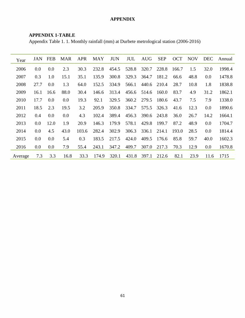
61
APPENDIX
APPENDIX 1-TABLE
Appendix Table 1. 1. Monthly rainfall (mm) at Durbete metrological station (2006-2016)
Year JAN FEB MAR APR MAY JUN JUL AUG SEP OCT NOV DEC Annual
2006 0.0 0.0 2.3 30.3 232.8 454.5 528.8 320.7 228.8 166.7 1.5 32.0 1998.4
2007 0.3 1.0 15.1 35.1 135.9 300.8 329.3 364.7 181.2 66.6 48.8 0.0 1478.8
2008 27.7 0.0 1.3 64.0 152.5 334.9 566.1 440.6 210.4 28.7 10.8 1.8 1838.8
2009 16.1 16.6 88.0 30.4 146.6 313.4 456.6 514.6 160.0 83.7 4.9 31.2 1862.1
2010 17.7 0.0 0.0 19.3 92.1 329.5 360.2 279.5 180.6 43.7 7.5 7.9 1338.0
2011 18.5 2.3 19.5 3.2 205.9 350.8 334.7 575.5 326.3 41.6 12.3 0.0 1890.6
2012 0.4 0.0 0.0 4.3 102.4 389.4 456.3 390.6 243.8 36.0 26.7 14.2 1664.1
2013 0.0 12.0 1.9 20.9 146.3 179.9 578.1 429.8 199.7 87.2 48.9 0.0 1704.7
2014 0.0 4.5 43.0 103.6 282.4 302.9 306.3 336.1 214.1 193.0 28.5 0.0 1814.4
2015 0.0 0.0 5.4 0.3 183.5 217.5 424.0 409.5 176.6 85.8 59.7 40.0 1602.3
2016 0.0 0.0 7.9 55.4 243.1 347.2 409.7 307.0 217.3 70.3 12.9 0.0 1670.8
Average 7.3 3.3 16.8 33.3 174.9 320.1 431.8 397.1 212.6 82.1 23.9 11.6 1715
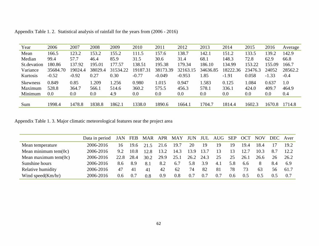
62
Appendix Table 1. 2. Statistical analysis of rainfall for the years from (2006 - 2016)
Year 2006 2007 2008 2009 2010 2011 2012 2013 2014 2015 2016 Average
Mean 166.5 123.2 153.2 155.2 111.5 157.6 138.7 142.1 151.2 133.5 139.2 142.9
Median 99.4 57.7 46.4 85.9 31.5 30.6 31.4 68.1 148.3 72.8 62.9 66.8
St.devation 180.86 137.92 195.01 177.57 138.51 195.38 179.34 186.10 134.99 153.22 155.09 166.7
Variance 35684.70 19024.4 38029.4 31534.22 19187.31 38173.39 32163.15 34636.85 18222.36 23476.3 24052 28562.2
Kurtosis -0.52 -0.92 0.27 0.30 -0.77 -0.049 -0.953 1.85 -1.91 0.058 -1.33 -0.4
Skewness 0.849 0.85 1.209 1.256 0.980 1.015 0.947 1.583 0.125 1.084 0.637 1.0
Maximum 528.8 364.7 566.1 514.6 360.2 575.5 456.3 578.1 336.1 424.0 409.7 464.9
Minimum 0.0 0.0 0.0 4.9 0.0 0.0 0.0 0.0 0.0 0.0 0.0 0.4
Sum 1998.4 1478.8 1838.8 1862.1 1338.0 1890.6 1664.1 1704.7 1814.4 1602.3 1670.8 1714.8
Appendix Table 1. 3. Major climatic meteorological features near the project area
Data in period JAN FEB MAR APR MAY JUN JUL AUG SEP OCT NOV DEC Aver
Mean temperature 2006-2016 16 19.6 21.5 21.6 19.7 20 19 19 19 19.4 18.4 17 19.2
Mean minimum tem(0c) 2006-2016 9.2 10.8 12.8 13.2 14.3 13.9 13.7 13 13 12.7 10.3 8.7 12.2
Mean maximum tem(0c) 2006-2016 22.8 28.4 30.2 29.9 25.1 26.2 24.3 25 25 26.1 26.6 26 26.2
Sunshine hours 2006-2016 8.6 8.9 8.1 8.2 6.7 5.8 3.9 4.1 5.8 6.6 8 8.4 6.9
Relative humidity 2006-2016 47 41 41 42 62 74 82 81 78 73 63 56 61.7
Wind speed(Km/hr) 2006-2016 0.6 0.7 0.8 0.9 0.8 0.7 0.7 0.7 0.6 0.5 0.5 0.5 0.7
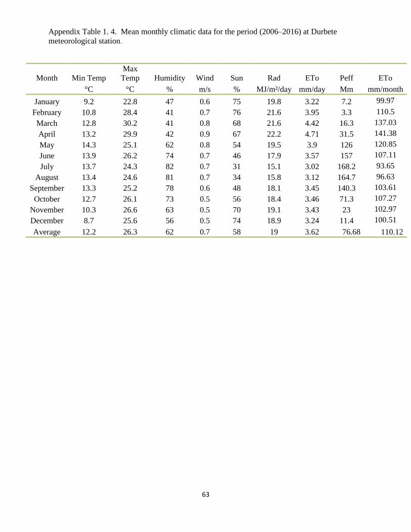
63
Appendix Table 1. 4. Mean monthly climatic data for the period (2006–2016) at Durbete
meteorological station.
Month Min Temp
Max
Temp Humidity Wind Sun Rad ETo Peff ETo
°C °C % m/s % MJ/m²/day mm/day Mm mm/month
January 9.2 22.8 47 0.6 75 19.8 3.22 7.2 99.97
February 10.8 28.4 41 0.7 76 21.6 3.95 3.3 110.5
March 12.8 30.2 41 0.8 68 21.6 4.42 16.3 137.03
April 13.2 29.9 42 0.9 67 22.2 4.71 31.5 141.38
May 14.3 25.1 62 0.8 54 19.5 3.9 126 120.85
June 13.9 26.2 74 0.7 46 17.9 3.57 157 107.11
July 13.7 24.3 82 0.7 31 15.1 3.02 168.2 93.65
August 13.4 24.6 81 0.7 34 15.8 3.12 164.7 96.63
September 13.3 25.2 78 0.6 48 18.1 3.45 140.3 103.61
October 12.7 26.1 73 0.5 56 18.4 3.46 71.3 107.27
November 10.3 26.6 63 0.5 70 19.1 3.43 23 102.97
December 8.7 25.6 56 0.5 74 18.9 3.24 11.4 100.51
Average 12.2 26.3 62 0.7 58 19 3.62 76.68 110.12
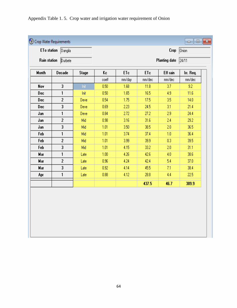
64
Appendix Table 1. 5. Crop water and irrigation water requirement of Onion
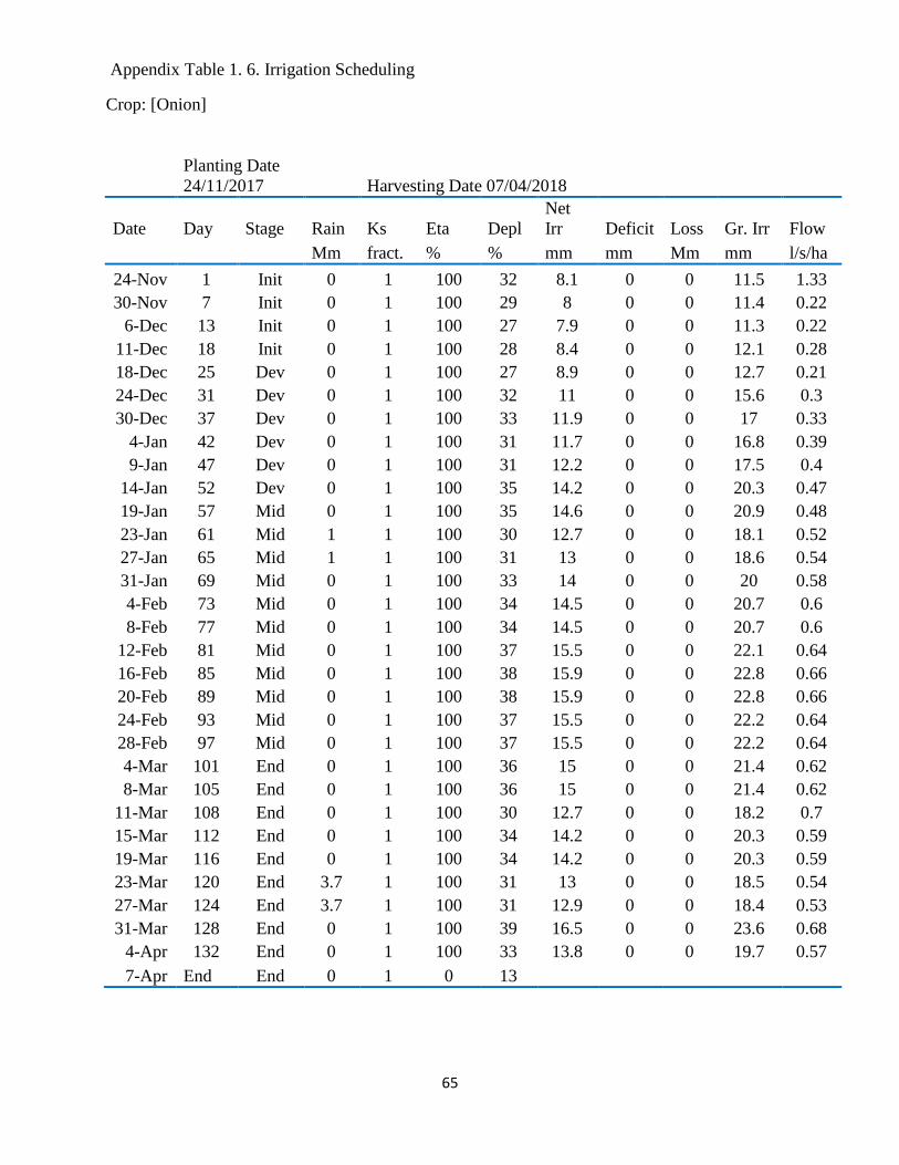
65
Appendix Table 1. 6. Irrigation Scheduling
Crop: [Onion]
Planting Date
24/11/2017 Harvesting Date 07/04/2018
Date Day Stage Rain Ks Eta Depl
Net
Irr Deficit Loss Gr. Irr Flow
Mm fract. % % mm mm Mm mm l/s/ha
24-Nov 1 Init 0 1 100 32 8.1 0 0 11.5 1.33
30-Nov 7 Init 0 1 100 29 8 0 0 11.4 0.22
6-Dec 13 Init 0 1 100 27 7.9 0 0 11.3 0.22
11-Dec 18 Init 0 1 100 28 8.4 0 0 12.1 0.28
18-Dec 25 Dev 0 1 100 27 8.9 0 0 12.7 0.21
24-Dec 31 Dev 0 1 100 32 11 0 0 15.6 0.3
30-Dec 37 Dev 0 1 100 33 11.9 0 0 17 0.33
4-Jan 42 Dev 0 1 100 31 11.7 0 0 16.8 0.39
9-Jan 47 Dev 0 1 100 31 12.2 0 0 17.5 0.4
14-Jan 52 Dev 0 1 100 35 14.2 0 0 20.3 0.47
19-Jan 57 Mid 0 1 100 35 14.6 0 0 20.9 0.48
23-Jan 61 Mid 1 1 100 30 12.7 0 0 18.1 0.52
27-Jan 65 Mid 1 1 100 31 13 0 0 18.6 0.54
31-Jan 69 Mid 0 1 100 33 14 0 0 20 0.58
4-Feb 73 Mid 0 1 100 34 14.5 0 0 20.7 0.6
8-Feb 77 Mid 0 1 100 34 14.5 0 0 20.7 0.6
12-Feb 81 Mid 0 1 100 37 15.5 0 0 22.1 0.64
16-Feb 85 Mid 0 1 100 38 15.9 0 0 22.8 0.66
20-Feb 89 Mid 0 1 100 38 15.9 0 0 22.8 0.66
24-Feb 93 Mid 0 1 100 37 15.5 0 0 22.2 0.64
28-Feb 97 Mid 0 1 100 37 15.5 0 0 22.2 0.64
4-Mar 101 End 0 1 100 36 15 0 0 21.4 0.62
8-Mar 105 End 0 1 100 36 15 0 0 21.4 0.62
11-Mar 108 End 0 1 100 30 12.7 0 0 18.2 0.7
15-Mar 112 End 0 1 100 34 14.2 0 0 20.3 0.59
19-Mar 116 End 0 1 100 34 14.2 0 0 20.3 0.59
23-Mar 120 End 3.7 1 100 31 13 0 0 18.5 0.54
27-Mar 124 End 3.7 1 100 31 12.9 0 0 18.4 0.53
31-Mar 128 End 0 1 100 39 16.5 0 0 23.6 0.68
4-Apr 132 End 0 1 100 33 13.8 0 0 19.7 0.57
7-Apr End End 0 1 0 13
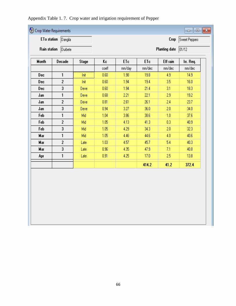
66
Appendix Table 1. 7. Crop water and irrigation requirement of Pepper
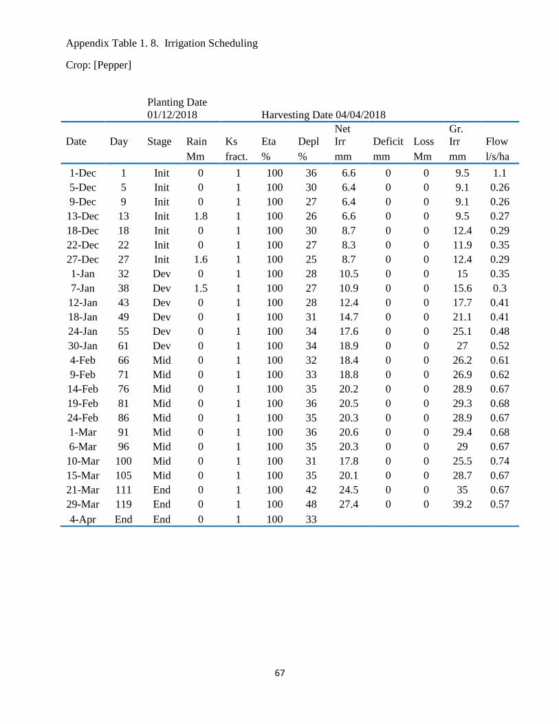
67
Appendix Table 1. 8. Irrigation Scheduling
Crop: [Pepper]
Planting Date
01/12/2018 Harvesting Date 04/04/2018
Date Day Stage Rain Ks Eta Depl
Net
Irr Deficit Loss
Gr.
Irr Flow
Mm fract. % % mm mm Mm mm l/s/ha
1-Dec 1 Init 0 1 100 36 6.6 0 0 9.5 1.1
5-Dec 5 Init 0 1 100 30 6.4 0 0 9.1 0.26
9-Dec 9 Init 0 1 100 27 6.4 0 0 9.1 0.26
13-Dec 13 Init 1.8 1 100 26 6.6 0 0 9.5 0.27
18-Dec 18 Init 0 1 100 30 8.7 0 0 12.4 0.29
22-Dec 22 Init 0 1 100 27 8.3 0 0 11.9 0.35
27-Dec 27 Init 1.6 1 100 25 8.7 0 0 12.4 0.29
1-Jan 32 Dev 0 1 100 28 10.5 0 0 15 0.35
7-Jan 38 Dev 1.5 1 100 27 10.9 0 0 15.6 0.3
12-Jan 43 Dev 0 1 100 28 12.4 0 0 17.7 0.41
18-Jan 49 Dev 0 1 100 31 14.7 0 0 21.1 0.41
24-Jan 55 Dev 0 1 100 34 17.6 0 0 25.1 0.48
30-Jan 61 Dev 0 1 100 34 18.9 0 0 27 0.52
4-Feb 66 Mid 0 1 100 32 18.4 0 0 26.2 0.61
9-Feb 71 Mid 0 1 100 33 18.8 0 0 26.9 0.62
14-Feb 76 Mid 0 1 100 35 20.2 0 0 28.9 0.67
19-Feb 81 Mid 0 1 100 36 20.5 0 0 29.3 0.68
24-Feb 86 Mid 0 1 100 35 20.3 0 0 28.9 0.67
1-Mar 91 Mid 0 1 100 36 20.6 0 0 29.4 0.68
6-Mar 96 Mid 0 1 100 35 20.3 0 0 29 0.67
10-Mar 100 Mid 0 1 100 31 17.8 0 0 25.5 0.74
15-Mar 105 Mid 0 1 100 35 20.1 0 0 28.7 0.67
21-Mar 111 End 0 1 100 42 24.5 0 0 35 0.67
29-Mar 119 End 0 1 100 48 27.4 0 0 39.2 0.57
4-Apr End End 0 1 100 33
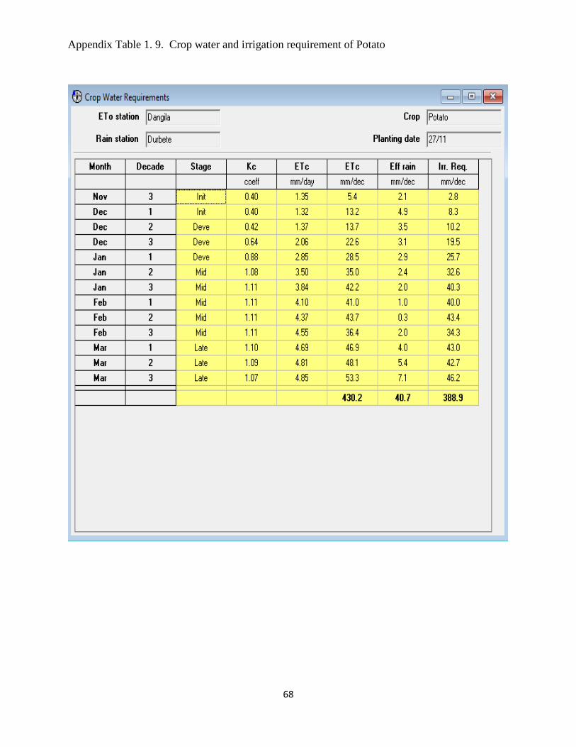
68
Appendix Table 1. 9. Crop water and irrigation requirement of Potato

69
Appendix Table 1. 10. Irrigation Scheduling
Crop: [Potato]
Planting Date
27/11/2017 Harvesting Date 31/03/2018
Date Day Stage Rain Ks Eta Depl
Net
Irr Deficit Loss
Gr.
Irr Flow
mm fract. % % mm mm Mm mm l/s/ha
28-Nov 2 Init 0 1 100 25 7.9 0 0 11.3 0.65
6-Dec 10 Init 0 1 100 26 8.8 0 0 12.5 0.18
14-Dec 18 Init 0 1 100 25 9.1 0 0 13 0.19
22-Dec 26 Dev 0 1 100 28 10.7 0 0 15.3 0.22
29-Dec 33 Dev 0 1 100 32 12.8 0 0 18.3 0.3
4-Jan 39 Dev 0 1 100 33 14.1 0 0 20.1 0.39
9-Jan 44 Dev 0 1 100 29 12.8 0 0 18.3 0.42
14-Jan 49 Dev 0 1 100 34 15.6 0 0 22.3 0.52
19-Jan 54 Mid 0 1 100 35 16.3 0 0 23.2 0.54
23-Jan 58 Mid 1 1 100 31 14 0 0 20 0.58
27-Jan 62 Mid 1 1 100 31 14.4 0 0 20.5 0.59
31-Jan 66 Mid 0 1 100 33 15.4 0 0 21.9 0.63
4-Feb 70 Mid 0 1 100 35 15.9 0 0 22.7 0.66
8-Feb 74 Mid 0 1 100 35 15.9 0 0 22.7 0.66
12-Feb 78 Mid 0 1 100 37 17 0 0 24.2 0.7
16-Feb 82 Mid 0 1 100 38 17.5 0 0 25 0.72
20-Feb 86 Mid 0 1 100 38 17.5 0 0 25 0.72
24-Feb 90 Mid 0 1 100 37 17.2 0 0 24.5 0.71
28-Feb 94 Mid 0 1 100 37 17.2 0 0 24.5 0.71
4-Mar 98 End 0 1 100 37 16.8 0 0 23.9 0.69
8-Mar 102 End 0 1 100 37 16.8 0 0 23.9 0.69
12-Mar 106 End 0 1 100 41 19 0 0 27.1 0.79
16-Mar 110 End 0 1 100 42 19.2 0 0 27.5 0.79
20-Mar 114 End 0 1 100 42 19.2 0 0 27.5 0.79
24-Mar 118 End 0 1 100 34 15.7 0 0 22.4 0.65
29-Mar 123 End 0 1 100 45 20.6 0 0 29.4 0.68
31-Mar End End 0 1 100 11
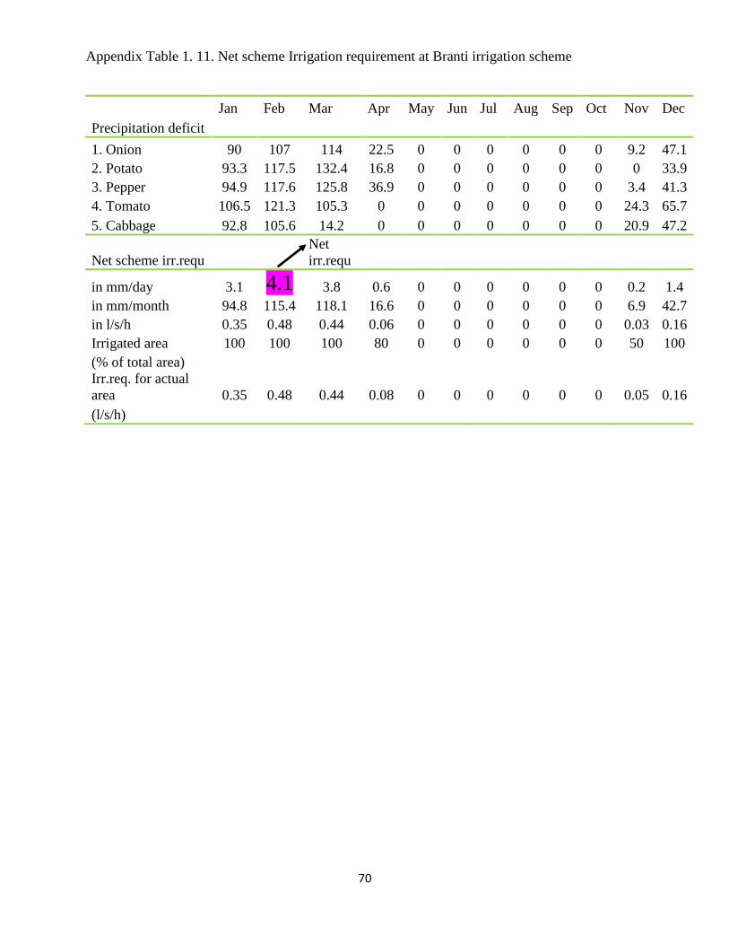
70
Appendix Table 1. 11. Net scheme Irrigation requirement at Branti irrigation scheme
Jan Feb Mar Apr May Jun Jul Aug Sep Oct Nov Dec
Precipitation deficit
1. Onion 90 107 114 22.5 0 0 0 0 0 0 9.2 47.1
2. Potato 93.3 117.5 132.4 16.8 0 0 0 0 0 0 0 33.9
3. Pepper 94.9 117.6 125.8 36.9 0 0 0 0 0 0 3.4 41.3
4. Tomato 106.5 121.3 105.3 0 0 0 0 0 0 0 24.3 65.7
5. Cabbage 92.8 105.6 14.2 0 0 0 0 0 0 0 20.9 47.2
Net scheme irr.requ Net
irr.requ
in mm/day 3.1 4.1 3.8 0.6 0 0 0 0 0 0 0.2 1.4
in mm/month 94.8 115.4 118.1 16.6 0 0 0 0 0 0 6.9 42.7
in l/s/h 0.35 0.48 0.44 0.06 0 0 0 0 0 0 0.03 0.16
Irrigated area 100 100 100 80 0 0 0 0 0 0 50 100
(% of total area)
Irr.req. for actual
area 0.35 0.48 0.44 0.08 0 0 0 0 0 0 0.05 0.16
(l/s/h)
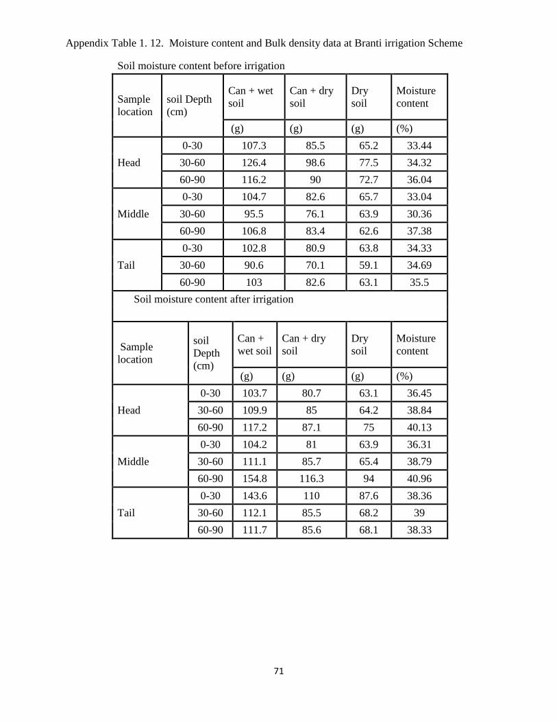
71
Appendix Table 1. 12. Moisture content and Bulk density data at Branti irrigation Scheme
Soil moisture content before irrigation
Sample
location
soil Depth
(cm)
Can + wet
soil
Can + dry
soil
Dry
soil
Moisture
content
(g) (g) (g) (%)
Head
0-30 107.3 85.5 65.2 33.44
30-60 126.4 98.6 77.5 34.32
60-90 116.2 90 72.7 36.04
Middle
0-30 104.7 82.6 65.7 33.04
30-60 95.5 76.1 63.9 30.36
60-90 106.8 83.4 62.6 37.38
Tail
0-30 102.8 80.9 63.8 34.33
30-60 90.6 70.1 59.1 34.69
60-90 103 82.6 63.1 35.5
Soil moisture content after irrigation
Sample
location
soil
Depth
(cm)
Can +
wet soil
Can + dry
soil
Dry
soil
Moisture
content
(g) (g) (g) (%)
Head
0-30 103.7 80.7 63.1 36.45
30-60 109.9 85 64.2 38.84
60-90 117.2 87.1 75 40.13
Middle
0-30 104.2 81 63.9 36.31
30-60 111.1 85.7 65.4 38.79
60-90 154.8 116.3 94 40.96
Tail
0-30 143.6 110 87.6 38.36
30-60 112.1 85.5 68.2 39
60-90 111.7 85.6 68.1 38.33
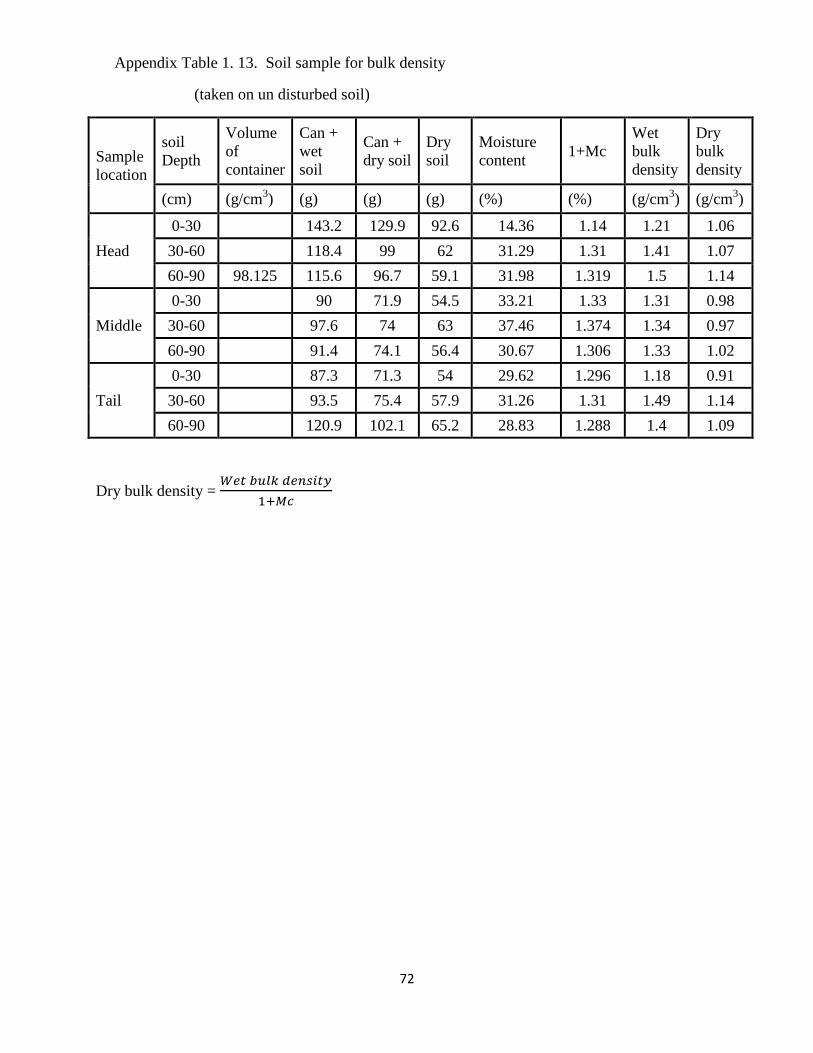
72
Appendix Table 1. 13. Soil sample for bulk density
(taken on un disturbed soil)
Sample
location
soil
Depth
Volume
of
container
Can +
wet
soil
Can +
dry soil
Dry
soil
Moisture
content 1+Mc
Wet
bulk
density
Dry
bulk
density
(cm) (g/cm3) (g) (g) (g) (%) (%) (g/cm
3) (g/cm
3)
Head
0-30 143.2 129.9 92.6 14.36 1.14 1.21 1.06
30-60 118.4 99 62 31.29 1.31 1.41 1.07
60-90 98.125 115.6 96.7 59.1 31.98 1.319 1.5 1.14
Middle
0-30 90 71.9 54.5 33.21 1.33 1.31 0.98
30-60 97.6 74 63 37.46 1.374 1.34 0.97
60-90 91.4 74.1 56.4 30.67 1.306 1.33 1.02
Tail
0-30 87.3 71.3 54 29.62 1.296 1.18 0.91
30-60 93.5 75.4 57.9 31.26 1.31 1.49 1.14
60-90 120.9 102.1 65.2 28.83 1.288 1.4 1.09
Dry bulk density =
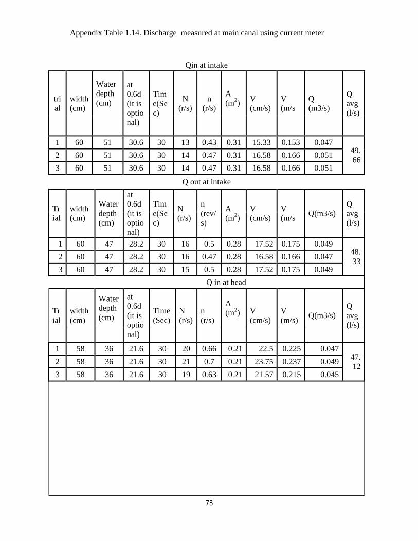
73
Appendix Table 1.14. Discharge measured at main canal using current meter
Qin at intake
tri
al
width
(cm)
Water
depth
(cm)
at
0.6d
(it is
optio
nal)
Tim
e(Se
c)
N
(r/s)
n
(r/s)
A
(m2)
V
(cm/s)
V
(m/s
Q
(m3/s)
Q
avg
(l/s)
1 60 51 30.6 30 13 0.43 0.31 15.33 0.153 0.047 49.
66 2 60 51 30.6 30 14 0.47 0.31 16.58 0.166 0.051
3 60 51 30.6 30 14 0.47 0.31 16.58 0.166 0.051
Q out at intake
Tr
ial
width
(cm)
Water
depth
(cm)
at
0.6d
(it is
optio
nal)
Tim
e(Se
c)
N
(r/s)
n
(rev/
s)
A
(m2)
V
(cm/s)
V
(m/s Q(m3/s)
Q
avg
(l/s)
1 60 47 28.2 30 16 0.5 0.28 17.52 0.175 0.049 48.
33 2 60 47 28.2 30 16 0.47 0.28 16.58 0.166 0.047
3 60 47 28.2 30 15 0.5 0.28 17.52 0.175 0.049
Q in at head
Tr
ial
width
(cm)
Water
depth
(cm)
at
0.6d
(it is
optio
nal)
Time
(Sec)
N
(r/s)
n
(r/s)
A
(m2)
V
(cm/s)
V
(m/s) Q(m3/s)
Q
avg
(l/s)
1 58 36 21.6 30 20 0.66 0.21 22.5 0.225 0.047
47.
12
2 58 36 21.6 30 21 0.7 0.21 23.75 0.237 0.049
3 58 36 21.6 30 19 0.63 0.21 21.57 0.215 0.045
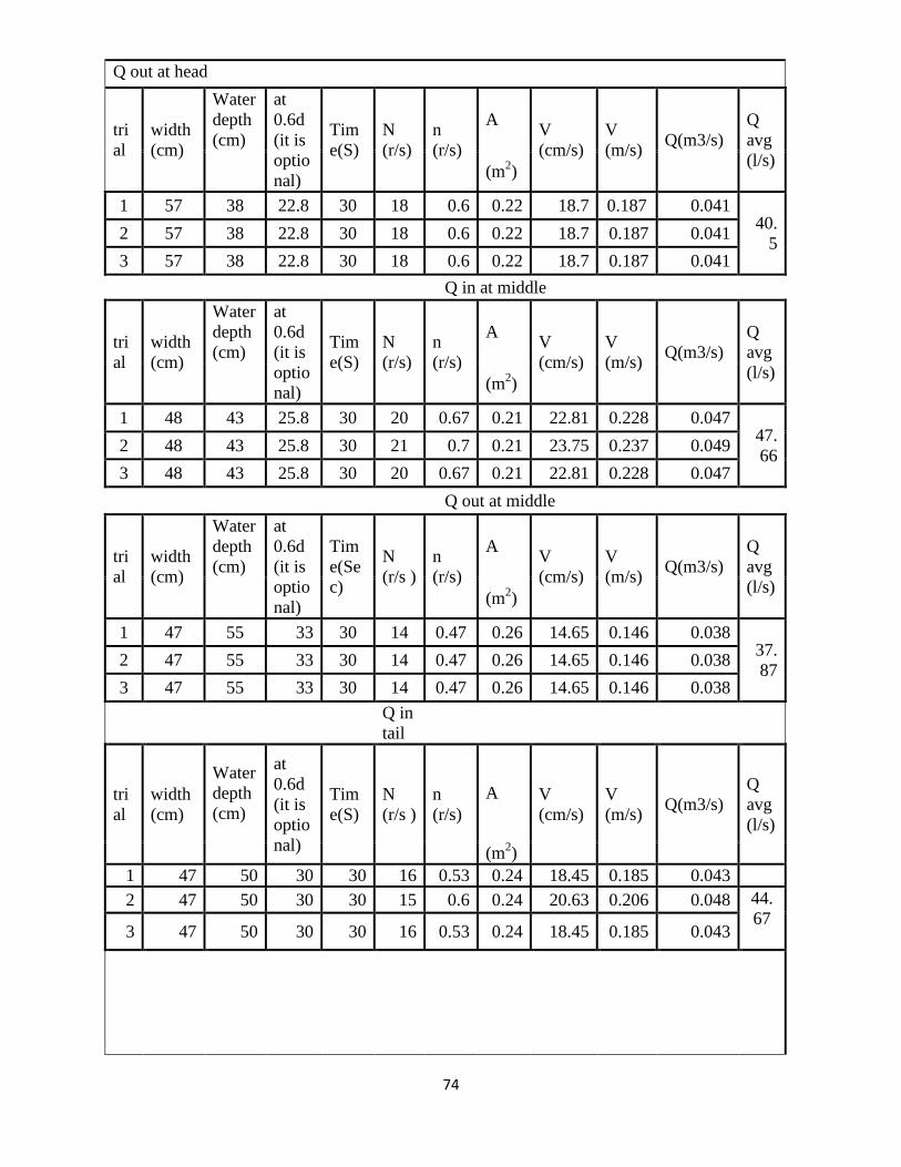
74
Q out at head
tri
al
width
(cm)
Water
depth
(cm)
at
0.6d
(it is
optio
nal)
Tim
e(S)
N
(r/s)
n
(r/s)
A V
(cm/s)
V
(m/s) Q(m3/s)
Q
avg
(l/s)
(m
2)
1 57 38 22.8 30 18 0.6 0.22 18.7 0.187 0.041 40.
5 2 57 38 22.8 30 18 0.6 0.22 18.7 0.187 0.041
3 57 38 22.8 30 18 0.6 0.22 18.7 0.187 0.041
Q in at middle
tri
al
width
(cm)
Water
depth
(cm)
at
0.6d
(it is
optio
nal)
Tim
e(S)
N
(r/s)
n
(r/s)
A V
(cm/s)
V
(m/s) Q(m3/s)
Q
avg
(l/s)
(m
2)
1 48 43 25.8 30 20 0.67 0.21 22.81 0.228 0.047 47.
66 2 48 43 25.8 30 21 0.7 0.21 23.75 0.237 0.049
3 48 43 25.8 30 20 0.67 0.21 22.81 0.228 0.047
Q out at middle
tri
al
width
(cm)
Water
depth
(cm)
at
0.6d
(it is
optio
nal)
Tim
e(Se
c)
N
(r/s )
n
(r/s)
A V
(cm/s)
V
(m/s) Q(m3/s)
Q
avg
(l/s)
(m
2)
1 47 55 33 30 14 0.47 0.26 14.65 0.146 0.038 37.
87 2 47 55 33 30 14 0.47 0.26 14.65 0.146 0.038
3 47 55 33 30 14 0.47 0.26 14.65 0.146 0.038
Q in
tail
tri
al
width
(cm)
Water
depth
(cm)
at
0.6d
(it is
optio
nal)
Tim
e(S)
N
(r/s )
n
(r/s)
A V
(cm/s)
V
(m/s) Q(m3/s)
Q
avg
(l/s)
(m2)
1 47 50 30 30 16 0.53 0.24 18.45 0.185 0.043
2 47 50 30 30 15 0.6 0.24 20.63 0.206 0.048 44.
67
3 47 50 30 30 16 0.53 0.24 18.45 0.185 0.043

75
Qout
tail
tri
al
width
(cm)
Water
depth(
cm)
at
0.6d
(it is
optio
nal)
Tim
e N
(r/s)
n
(r/s)
A
(m2)
V
(cm/s)
V
(m/s)
Q Q
avg
(l/s)
(S) (m3/s)
1 47 45 27 30 17 0.57 0.21 19.69 0.197 0.041
41.
67
2 47 45 27 30 18 0.6 0.21 20.63 0.206 0.043
3 47 45 27 30 17 0.57 0.21 19.69 0.197 0.041
Appendix Table 1.15. Discharge data measured at Secondary canal using current meter
Q in at SC1
tri
al
width
(cm)
Water
depth
at
0.6d
(it is
optio
nal)
Tim
e(Se
c)
N
(r/s)
n
(r/s)
A V
(cm/s)
V
(m/s) Q(m3/s)
Q
avg
(l/s) (cm) (m
2)
1 50 14 7.2 30 23 0.77 0.07 25.8 0.258 0.018
17.
70
2 50 14 7.2 30 23 0.77 0.07 25.8 0.258 0.018
3 50 14 7.2 30 22 0.73 0.07 24.77 0.248 0.017
Q out at SC1
tri
al
width
(cm)
Water
depth,
(cm)
at
0.6d
(it is
optio
nal)
Tim
e(Se
c)
N
(r/s)
n
(r/s)
A
(m2)
V
(cm/s)
V
(m/s) Q(m3/s)
Q
avg
(l/s)
1 40 18 10.8 30 18 0.6 0.07 20.63 0.206 0.015
14.
67
2 40 18 10.8 30 17 0.57 0.07 19.69 0.197 0.014
3 40 18 10.8 30 18 0.6 0.07 20.63 0.206 0.015
Q in at SC2
tri
al
width
(cm)
Water
depth
(cm)
at
0.6d
(it is
optio
nal)
Tim
e(Se
c)
N
(r/s)
n
(r/s)
A V
(cm/s)
V
(m/s) Q(m3/s)
Q
avg
(l/s)
(m
2)
1 50 14 7.2 30 23 0.77 0.07 25.8 0.258 0.018
16.
50
2 50 14 7.2 30 23 0.77 0.07 25.8 0.258 0.018
3 50 14 7.2 30 22 0.73 0.07 24.77 0.248 0.017
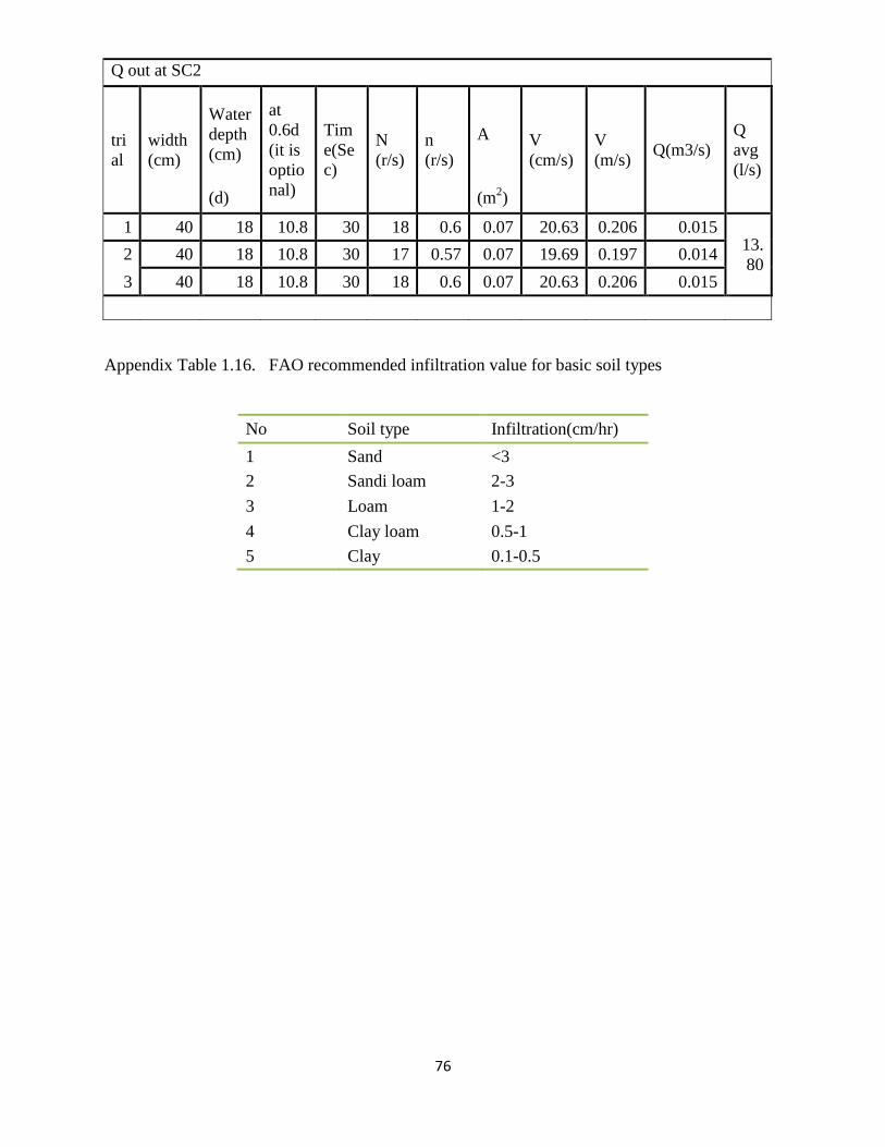
76
Q out at SC2
tri
al
width
(cm)
Water
depth
(cm)
at
0.6d
(it is
optio
nal)
Tim
e(Se
c)
N
(r/s)
n
(r/s)
A V
(cm/s)
V
(m/s) Q(m3/s)
Q
avg
(l/s)
(d) (m2)
1 40 18 10.8 30 18 0.6 0.07 20.63 0.206 0.015
13.
80
2 40 18 10.8 30 17 0.57 0.07 19.69 0.197 0.014
3 40 18 10.8 30 18 0.6 0.07 20.63 0.206 0.015
Appendix Table 1.16. FAO recommended infiltration value for basic soil types
No Soil type Infiltration(cm/hr)
1 Sand <3
2 Sandi loam 2-3
3 Loam 1-2
4 Clay loam 0.5-1
5 Clay 0.1-0.5
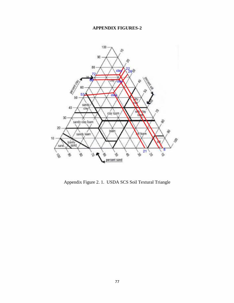
77
APPENDIX FIGURES-2
Appendix Figure 2. 1. USDA SCS Soil Textural Triangle
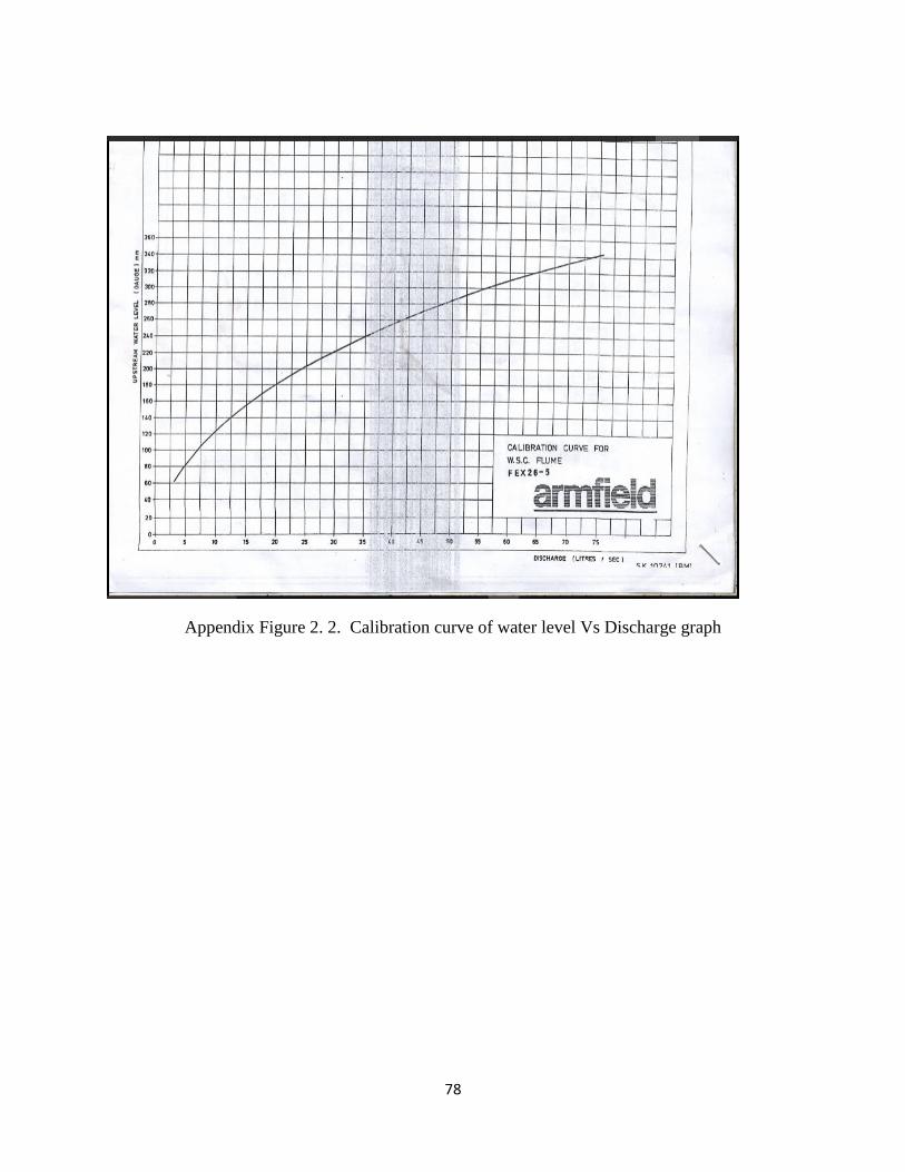
78
Appendix Figure 2. 2. Calibration curve of water level Vs Discharge graph
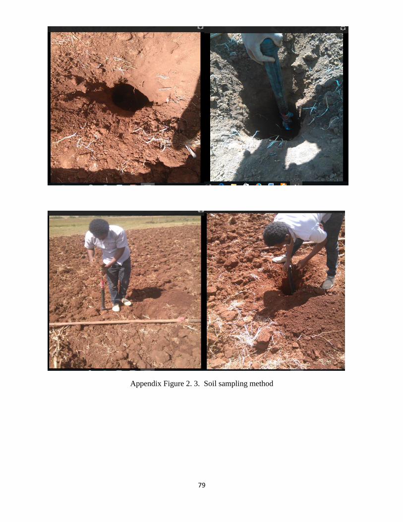
79
Appendix Figure 2. 3. Soil sampling method
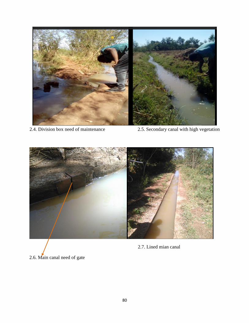
80
2.4. Division box need of maintenance 2.5. Secondary canal with high vegetation
2.7. Lined mian canal
2.6. Main canal need of gate

81
APPENDIX-3 QUESTIONER
ANNEX I: QUESTIONNAIRE FOR
RANDOMLY SELECTED
IRRIGATION USER FARMERS OF BRANTI IRRIGATION
SCHEME
Dear respondent, my name is Getachew Kelemework from Bahir Dar University, Ethiopia. I
am conducted a study on performance evaluation of small scale irrigation scheme: a case
study of Branti irrigation scheme. The main objective of this questionnaire is to recognize the
water management practice from farmer perspective and institutional set up of Water users
association. Therefore, I am kindly requesting you to give a response as much as you can. All the
questioner targets on the head, middle and tail reaches of the scheme and collects at household
level and group discussion. The choice of participant (respondent) is made randomly using
simple random sampling technique.
A) Socio-economic characteristics of the Respondent
1. Household head Male Female
2. Educational level_________________
3. Do you think the project was important in your area? Yes No
4. If yes, has the use of irrigation increased your annual income and livelihood? Yes No
5. If yes, what is the estimated proportion of increment in the amount of income from crops?
Compared to before the project time? ______________ %
6. Who manages and control the irrigation water?
1. The community as a whole
2. Representatives of the community
3. Devlopment agents (DA)
4. Others (Specify): _____________
7. Is there any conflict in the scheme? Yes No

82
8. If yes, what are the common source(s) of conflicts?
1. Water shortage
2. Water theft
3. Illegal water abstraction
4. Others (specify) ---------------
9. Is water equally available to all users in the scheme? Yes No
10. Is there problem of water theft or unauthorized canal breaching? Yes No
11. Do you foresee any conflict on the water use in the future? Yes No
If yes, what will be the causes? _____________
12. What should be done to avoid the conflict? _____________
B) Project Evaluation
I. planning
1. Who initiate the idea of constructing the structures?
1. Local people
2. DA
3. Project staff
4. Others____________
2. If it is not the local people, have you agreed about the construction of the structures? Yes No
3. Have you been consulted for the construction? Yes No
4. How was the planning process?
1. Group discussion
2. Simple information by DAs
3. Simple information by PA leader
4. Simple information by project personnel
5. Have you participate in planning of any project? Yes No

83
II. Design/ layout/construction
1. Who design or put the layout of the structure?
1. DA
2. Project staff
3. Woreda expert
2. Were you agreed on the project/dam site? Yes No
3. What is your opinion about canal design and dam site? ___________
4. Did you face any problem because of the site selection? Yes No
If yes, what was the problem? ________________
III Implementation
1. Have you participate in canal and diversion structure construction? Yes No
If yes, how is your way of participation? ____________
2. Do you use the irrigation project by now? Yes No
If No, why? __________________
3. Do you know the cause of failure? Yes No
If yes, what are they?
1. Seepage from the head work and/or the canals and its structure
2. Structural failure
3. Design problem
4. Sedimentation problem
4. Do you expect these failures? Yes No
If yes, why? ______________
5. Do you see any structural failure? Yes No
If yes, which structures?
1. The head work
2. The spillway
3. The canal structures
4. All
5. Other structures (indicate)__________
6. Do you see any seepage on the headwork, canals and canal structures? Yes No

84
C) Organizations
1. Is there water users association in your locality? Yes No
2. If yes, are you a member of water users association? Yes No
3. If yes, how was the association formed? ___________
D) Water management
1. What criteria should you used to decide when to irrigated crops?
1. Wait until see signs of wilting on the leaves
2. Check the soil near the roots
3. When it is dry, I irrigate
4. Irrigate every day
2. Do you think your yield is reduced because you cannot apply enough water to your crop? Yes
No
3. Who makes decisions on the sequence of using irrigation water? ___________
4. What is the system of water allocation?
1. Proportional to the amount of land you have under irrigation.
2. Equal division among members of the association
3. Specify if any other system_______________
5. Does the community have a system of rule for controlling water distribution default? Yes No
6. Are there special considerations for crop-type and stage of growth during water allocation?
Yes No
7. Have you trained how to use water in the scheme? Yes No
E) Sustainability of the project
1. Do you feel that the irrigation scheme belongs to you? Yes No
2. If No, whom do you think it belongs to?
1. To the community
2. To the government
3. To the NGOs
4. Any combination of the above_____________
3. Have you ever participated in operation and maintenance of the irrigation canal? Yes No
4. If you do not make the maintenance, what is the reason?
1. It is not my responsibility
2. I do not know how it is done
3. Others (specify)_______________
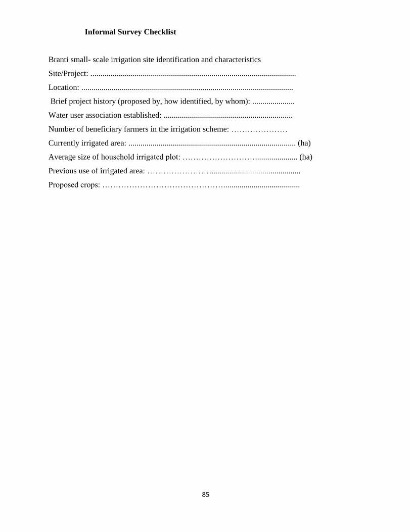
85
Informal Survey Checklist
Branti small- scale irrigation site identification and characteristics
Site/Project: ......................................................................................................
Location: .........................................................................................................
Brief project history (proposed by, how identified, by whom): .....................
Water user association established: ................................................................
Number of beneficiary farmers in the irrigation scheme: …………………
Currently irrigated area: ................................................................................... (ha)
Average size of household irrigated plot: ………………………..................... (ha)
Previous use of irrigated area: ……………………............................................
Proposed crops: ………………………………………......................................


