Alma Mater Studiorum · Universita di Bologna

Scuola di Scienze

Corso di Laurea Magistrale in Fisica

PERFORMANCE EVALUATIONOF DETECTOR FOR

DIGITAL RADIOGRAPHY

Relatore:Prof.Romano Zannoli

Correlatore:Dott.David Bianchini

Presentata da:Maria Celeste Maschio

Sessione III

Anno Accademico 2013-2014

ii

ABSTRACT

Lo scopo di questo lavoro è la caratterizzazione fisica del flat panel PaxScan4030CB

Varian, rivelatore di raggi X impiegato in un ampio spettro di applicazioni cliniche, dalla

radiografia generale alla radiologia interventistica.

Nell’ambito clinico, al fine di una diagnosi accurata, è necessario avere una buona

qualità dell’immagine radiologica mantenendo il più basso livello di dose rilasciata al

paziente.

Elemento fondamentale per ottenere questo risultato è la scelta del rivelatore di

radiazione X, che deve garantire prestazioni fisiche (contrasto, risoluzione spaziale e rumore)

adeguati alla specifica procedura. Le metriche oggettive che misurano queste caratteristiche

sono SNR (Signal-to-Noise Ratio), MTF (Modulation Transfer Function) ed NPS (Noise

Power Spectrum), che insieme contribuiscono alla misura della DQE (Detective Quantum

Efficiency), il parametro più completo e adatto a stabilire le performance di un sistema di

imaging. L’oggettività di queste misure consente anche di mettere a confronto tra loro

diversi sistemi di rivelazione.

La misura di questi parametri deve essere effettuata seguendo precisi protocolli di fisica

medica, che sono stati applicati al rivelatore PaxScan4030CB presente nel laboratorio del

Centro di Coordinamento di Fisica Medica, Policlinico S.Orsola.

I risultati ottenuti, conformi a quelli dichiarati dal costruttore, sono stati confrontati

con successo con alcuni lavori presenti in letteratura e costituiscono la base necessaria per la

verifica di procedure di ottimizzazione dell’immagine radiologica attraverso interventi sul

processo di emissione dei raggi X e sul trattamento informatico dell’immagine (Digital

Subtraction Angiography).

iii

iv

OVERVIEW

The present work deals with the physical characterization of the flat panel

PaxScan4030CB Varian, which is a part of the fluoroscopic chain present in the laboratory

of the Centre of Medical Physics at the Policlinico S.Orsola.

The work is structured as follows: in Chapter 1, the main features of the flat panel

technology are reported and the basic image quality parameters, such as MTF, NPS and

DQE, are described in order to get an overview on the image quality issue.

In Chapter 2, the principal characteristics of X-ray source RTM70H and its generator

are emphasized; the flat panel is illustrated in detail in its physical (i.e. the scintillator) and

electronic constituents, with particular attention to the pre-processing corrections. Then, the

main steps in image quality parameters calculation are reported, and the employed dosimeter

and phantom are described.

In Chapter 3, standard RQA beams are recreated from the RTM70H in order to

perform a physical characterization of the PaxScan4030CB. MTF, NPS and DQE are

evaluated from the acquired images and then, in conclusion, successfully compared with

other results in literature.

v

vi

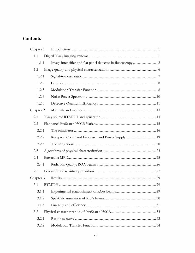
Contents

Chapter 1 Introduction ....................................................................................................... 1

1.1 Digital X-ray imaging systems .................................................................................. 1

1.1.1 Image intensifier and flat panel detector in fluoroscopy ............................. 2

1.2 Image quality and physical characterization ........................................................... 6

1.2.1 Signal-to-noise ratio ........................................................................................... 7

1.2.2 Contrast ............................................................................................................... 8

1.2.3 Modulation Transfer Function ........................................................................ 8

1.2.4 Noise Power Spectrum ................................................................................... 10

1.2.5 Detective Quantum Efficiency ...................................................................... 11

Chapter 2 Materials and methods .................................................................................... 13

2.1 X-ray source RTM70H and generator .................................................................. 13

2.2 Flat panel PaxScan 4030CB Varian ....................................................................... 15

2.2.1 The scintillator ................................................................................................. 16

2.2.2 Receptor, Command Processor and Power Supply.................................... 19

2.2.3 The corrections ................................................................................................ 20

2.3 Algorithms of physical characterization ............................................................... 23

2.4 Barracuda MPD........................................................................................................ 25

2.4.1 Radiation quality: RQA beams ...................................................................... 26

2.5 Low-contrast sensitivity phantom ......................................................................... 27

Chapter 3 Results ............................................................................................................... 29

3.1 RTM70H ................................................................................................................... 29

3.1.1 Experimental establishment of RQA beams ............................................... 29

3.1.2 SpekCalc simulation of RQA beams ............................................................ 30

3.1.3 Linearity and efficiency ................................................................................... 31

3.2 Physical characterization of PaxScan 4030CB ..................................................... 33

3.2.1 Response curve ................................................................................................ 33

3.2.2 Modulation Transfer Function ...................................................................... 34

vii

3.2.3 Noise Power Spectrum .................................................................................... 36

3.2.4 Detective Quantum Efficiency ....................................................................... 38

3.3 Phantoms and contrast ............................................................................................ 40

3.5 Flat panel detectors in literature ............................................................................. 42

Chapter 4 Conclusions ....................................................................................................... 47

Bibliography ............................................................................................................................... 49

1

Chapter 1 Introduction

1.1 Digital X-ray imaging systems

The power of X-rays for medical imaging is invaluable, but as a form of ionizing

radiation presents a risk to the patient. It is then essential that the benefits to the patient

overcome the costs in terms of biological risks. For X-ray imaging procedures, the principle

of ALARA (As Low As Reasonable Achievable) is observed and requires that patient

equivalent dose be minimized as much as possible without compromising diagnostic

benefits of the examination.

The statistical nature of X-ray interactions results in image noise when too few X-ray

photons are used to create the image. Hence, there is a fundamental trade-off between

patient dose (number of quanta) and image quality. The optimal balance strictly depends on

X-rays detectors, that have to be designed in order to produce the best image quality for

every radiation exposure. When the visualization of small structures and fine lesions is

required, not all the X-ray systems provide the optimal balance to the patients [1].

With the evolution of digital imaging, there are new ways of optimizing the X-ray image

and reducing the dose to the patient. The most fundamental goal of digital imaging is

reached by flat panel detector, a single technology that covers all applications in X-ray

diagnostics and interventional techniques, from general radiography to angiography and

fluoroscopy.

In order to evaluate and describe the performance of a X-ray flat panel detector, it is

commonly acknowledged that the detective quantum efficiency (DQE) is the most suitable

parameter that describes how close a detector is to the optimal balance of image quality and

exposure, combining the spatial resolution (MTF) and image noise (NPS).

In this work, we are interested in the performance evaluation of the flat panel that is

part of the fluoroscopic chain of our laboratory at the Centre of Medical Physics, Policlinico

S.Orsola. This first chapter gives an overview on technological evolution of X-ray imaging

and basic image quality parameters.

2

1.1.1 Image intensifier and flat panel detector in

fluoroscopy

Fluoroscopy allows real-time viewing of the patient with high-acquisition-frame rate

and it is, in essence, real-time radiography. During fluoroscopic procedures, very high doses

are released to the patient because of the duration of this medical exam (sometimes more

than one hour). Because of factors that depend mainly on the patient, it’s not always

possible reduce the length of time of these procedures and so physicians typically adopt low-

radiation exposure rates [2]. This choice has negative outcomes on the images, that become

noisier and don’t permit to distinguish minute details of the blood vessels and the needles,

catheters and other angiographical equipments.

In the early period, image intensifier was the principal component of the fluoroscopic

chain. This instrument represented a big revolution with respect to the screen-film cassette,

because of its higher sensitivity to radiation. Using conversion scintillator layers and

focusing electrodes inside a vacuum tube, the X-ray image intensifier (XRII) turns a low X-

ray photon fluence emerging from the patients to high fluence of visible photons. XRII are

coupled with video camera, used to capture the image in output, that is the conversion of

the X-ray intensity in electronic signal [3]. Medical systems based on X-ray image intensifier

have several disadvantages: wide structure of the intensifier often limits the clinicians during

the access to the patient; X-ray and light scatter inside the intensifier produce losses of

image contrast; severe distortions of the image largely occurs because of the curved input

scintillators (geometrical distortion) and because of the Earth’s magnetic field (S distortion)

[4].

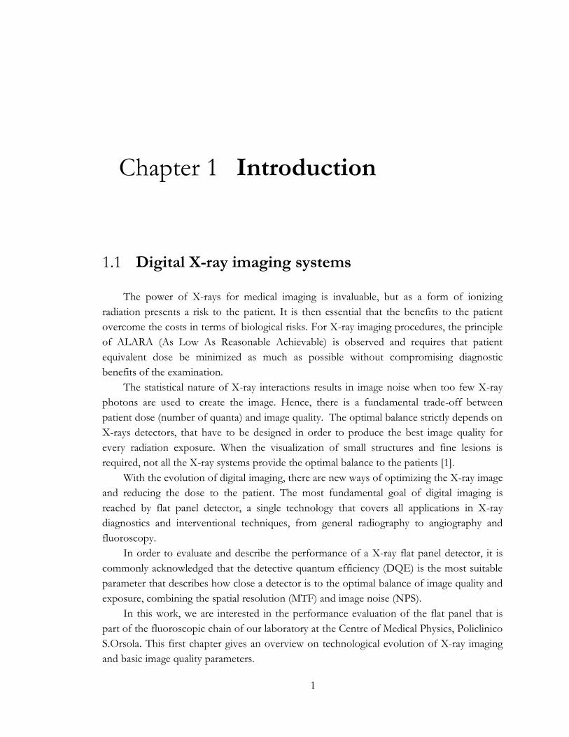
Another limitation of the XRII is the dynamic range (Figure 1-1): XRIIs saturate at high

radiation levels or if only a portion of the incident beam passes through a low-density

anatomy, such lung or external air, causing the veiling glare [5]; on the other hand, low

radiation levels are displayed at quite the same brightness on the monitor.

Although all these restrictions, XRIIs performed very well in medical applications for

many decades, but the evolution of the imaging technology has brought to flat panel

detectors (FPDs), that have sensibly improved the fluoroscopic procedure: in fact, an active-

matrix panel is compact, flat, free of veiling glare and geometrically uniform thanks to the

larger dynamic range (Figure 1-1) which better displays the various radiation levels

transmitted to the patient.

The principal requirement for the X-ray detectors is to efficiently absorb the impinging

X-ray beam and to convert it into a digital image. During this process, the X-ray signal

should be maximized while the additive electronic noise has to be kept at minimum. The

3

main features of a detector are influenced by many design criteria, like active area, pixel size,

image acquisition rate, dynamic range and also outer dimensions and weight. Each detector

Figure 1-1: graph plots of the dynamic ranges of an image intensifier(dashed line) and FPD(solid line)

fluoroscopy system [5].

application requires different characteristics for each parameters and only flat panel

detectors are characterized by a technology that entirely covers the needs of different

application, from general radiography to angiography and fluoroscopy [6].

The four main stages of the creation of an X-ray image are: interaction of the X-ray

quanta with a detection medium to generate a sensible response; storage of this response in

a recording device; measurement of the stored response; erasure [3].

To generate a sensible response, two different conversion processes of X-ray radiation

into electric charge prevail: the first approach is based on an indirect conversion process,

where the X-ray photons are converted into light, which in turn is absorbed creating electric

charge. The second approach is the direct conversion of X-ray quanta into electric charge.

For flat panel based on indirect conversion process, the thallium-doped cesium iodide

(CsI(Tl)) and the gadolinium oxysulfide (Gd2O2S) are the most common used scintillators.

The studied detector in this thesis work is made of CsI(Tl). This scintillator can be grown as

needle-shaped crystals with diameter of 5-10 µm which act like a light-guide and diminish

the lateral spread of the light. Another important feature of the crystal is good X-ray

absorption property, due to high atomic number of cesium (Z=55) and iodide (Z=53). The

X-ray applications like general radiography, angiography and fluoroscopy cover a range from

45 kVp to 120 kVp, where the absorption peaks of CsI(Tl) and Gd2O2S are comprised.

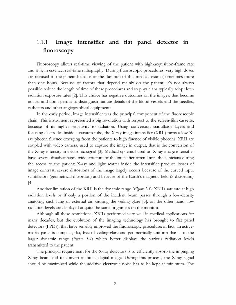
In Figure 1-2 the cross sections of the two cited scintillators are reported, in comparison

with the amorphous selenium (a-Se). This material is the most used photoconductor layer in

the direct conversion process, and in particular is more adapt to mammography than

fluoroscopy because of its absorption edge at very low energy.

Both CsI scintillator and a-Se layer can be read-out by a large area of activated circuits

called active matrix arrays (AMA), with millions of pixels. This type of technology allows the

deposition of semiconductors, most commonly amorphous silicon (a-Si), across a large area

4

substrates in a such manner that the physical and electrical properties of the resulting

structure can be adapted for many different applications.

Figure 1-2: absorption coefficients of CsI, a-Se and Gd2O2S as a function of X-ray photon energy [7].

Sensors in X-ray medical imaging find a valid aid in amorphous silicon, because it

combines favorable characteristics: a-Si exhibits all of the semiconductor properties,

becoming suitable for the manufacture of electrical components, like thin-film transistors

(TFT) and photodiode, and furthermore a-Si has proven to be highly radiation hard, making

it appropriate for medical X-ray imaging.

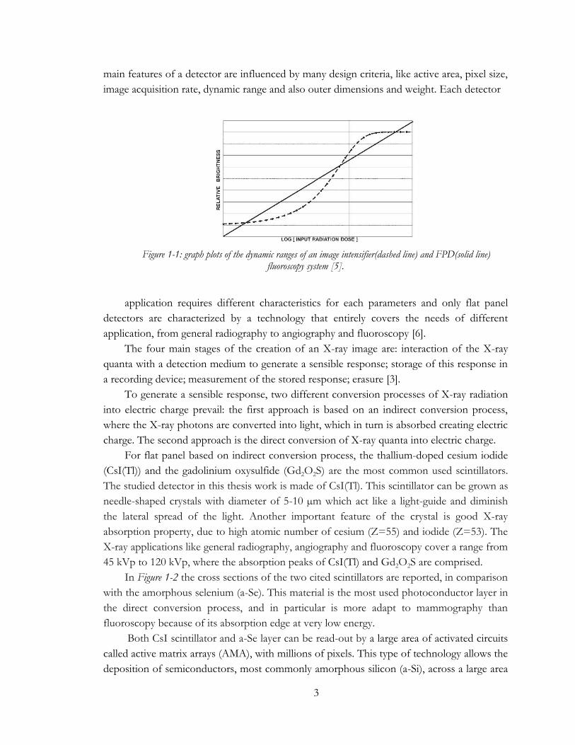
In the indirect conversion process, as schematically reported in Figure 1-3, after the X-

ray beam is photo-absorbed, the created high-energy electron loses its energy in the

scintillator material and creates a large number or electron-hole pairs. These couples

recombine themselves to produce photons in the visible range. Then the photodiode,

constructed to reach the highest quantum efficiency in the same part of the spectrum of the

scintillator light, captures this light and converts it into electric charge.

Figure 1-3: schematics of the indirect conversion process [7].

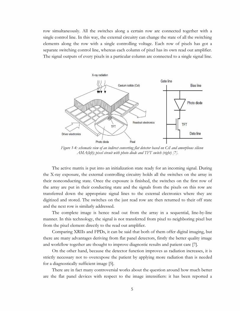
To acquire and read out a radiographic image, the structure of the active matrix and the

electric circuit for a TFT-based pixel structure (Figure 1-4) works as follow. The readout of

the stored electric charge is performed row by row and addresses all pixels in the respective

5

row simultaneously. All the switches along a certain row are connected together with a

single control line. In this way, the external circuitry can change the state of all the switching

elements along the row with a single controlling voltage. Each row of pixels has got a

separate switching control line, whereas each column of pixel has its own read out amplifier.

The signal outputs of every pixels in a particular column are connected to a single signal line.

Figure 1-4: schematic view of an indirect converting flat detector based on CsI and amorphous silicon

AMA(left); pixel circuit with photo diode and TFT switch (right) [7].

The active matrix is put into an initialization state ready for an incoming signal. During

the X-ray exposure, the external controlling circuitry holds all the switches on the array in

their nonconducting state. Once the exposure is finished, the switches on the first row of

the array are put in their conducting state and the signals from the pixels on this row are

transferred down the appropriate signal lines to the external electronics where they are

digitized and stored. The switches on the just read row are then returned to their off state

and the next row is similarly addressed.

The complete image is hence read out from the array in a sequential, line-by-line

manner. In this technology, the signal is not transferred from pixel to neighboring pixel but

from the pixel element directly to the read out amplifier.

Comparing XRIIs and FPDs, it can be said that both of them offer digital imaging, but

there are many advantages deriving from flat panel detectors, firstly the better quality image

and workflow together are thought to improve diagnostic results and patient care [7].

On the other hand, because the detector function improves as radiation increases, it is

strictly necessary not to overexpose the patient by applying more radiation than is needed

for a diagnostically sufficient image [5].

There are in fact many controversial works about the question around how much better

are the flat panel devices with respect to the image intensifiers: it has been reported a

6

remarkable dose reduction (up to 80%) and a large increasing in the image quality (up to 2.5

times) with the use of FPD system [8, 9]. But other experiments have stated that the choice

of FPD systems do not assure automatically an improvement in image quality or in dose

efficiency over the II systems [9, 10]. In the end, for both the technologies, some studies

reported similar experimental results, comparing visibility scores and dose-area product [9].

1.2 Image quality and physical characterization

In medical imaging, the concept of image quality is intrinsically related to diagnosis

made by the radiologist. The body part being imaged is processed through a digital system

and, in this way, distortions or artifacts are introduced in the output image.

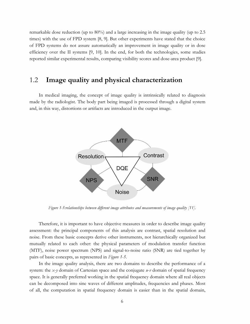
Figure 1-5:relationships between different image attributes and measurements of image quality [11].

Therefore, it is important to have objective measures in order to describe image quality

assessment: the principal components of this analysis are contrast, spatial resolution and

noise. From these basic concepts derive other instruments, not hierarchically organized but

mutually related to each other: the physical parameters of modulation transfer function

(MTF), noise power spectrum (NPS) and signal-to-noise ratio (SNR) are tied together by

pairs of basic concepts, as represented in Figure 1-5.

In the image quality analysis, there are two domains to describe the performance of a

system: the x-y domain of Cartesian space and the conjugate u-v domain of spatial frequency

space. It is generally preferred working in the spatial frequency domain where all real objects

can be decomposed into sine waves of different amplitudes, frequencies and phases. Most

of all, the computation in spatial frequency domain is easier than in the spatial domain,

7

because multiplication is used instead of convolution. The MTF, NPS and DQE are hence

studied in the spatial frequency domain.

1.2.1 Signal-to-noise ratio

One of the most relevant image quality factor in X-ray imaging is the signal-to-noise

ratio (SNR), that carries the importance of signal sensitivity and image-noise properties.

Considering a number N of detected X-ray photons and a stochastic signal fluctuation

according to the Poisson statistics, i.e. the square root of the detected signal, the signal-to-

noise ratio is given by:

𝑆𝑁𝑅 = √𝑁

It can be immediately observed that, as N increases in an image, the SNR increases as

well, improving the image quality. But this growth leads also to a higher entrance dose. In

fact, improving SNR means increasing the patient dose of a large factor: with some simple

calculations, it can be seen that to double SNR, the patient dose has to be increased by a

factor of 4. Generally, in medical X-ray imaging, the interest is to reduce the patient dose, so

there has to exist a trade-off between SNR and radiation dose.

The image quality of X-ray imaging system is strongly dependent on the number of

quanta used to produce an image [4, 12], so an ideal X-ray detector should count every

single photon that reaches its surface, as it contributes to the SNR. But in reality detectors

generally don’t absorb all the incident X-ray and hence the SNR is degraded. The upper limit

of SNR is given by the quantum noise, that refers to the statistical variation in the number

of detected quanta.

The quantum detection efficiency (QDE) is the ratio of the number of detected X-ray

photons (Nabsorbed) to the number of incident photons (Nincident) for a certain detector. So,

considering a real detector, the image SNR depends on the number of detected photons:

𝑆𝑁𝑅𝑟𝑒𝑎𝑙 = √𝑁𝑑𝑒𝑡𝑒𝑐𝑡𝑒𝑑 = √𝑄𝐷𝐸 ∙ 𝑁𝑖𝑛𝑐𝑖𝑑𝑒𝑛𝑡

QDE increases if the detection layer thickness increases. However, it is not true that

detector with the highest QDE produce images with the highest SNR for a given dose.

There are in fact other physical processes in the detector that may reduce the SNR. The

concept of DQE describes SNR in terms of an effective quantum efficiency, that is the

effective fraction of X-ray quanta contributing to image SNR taking into account additional

noise introduced by the detector.

8

1.2.2 Contrast

The contrast in an image defines the difference of the gray level between two adjacent

areas, hence the discrimination between two different structures of the body anatomy

irradiated with the X-ray beam. In a radiographic image, the inherent contrast refers to the

contrast of intensity patterns before application of image processing and displaying. It

depends on several factors: beam spectrum and energy response of the detector, variation of

the thickness and composition of the object being imaged and scattered radiation.

The response of the detector also has a role in determining the contrast of objects: in

case of poor response at higher photon energies, the contrast will be further reduced after

the tissues attenuation.

The contrast of an object relative to its background is defined as:

𝐶 =𝐼𝑏 − 𝐼

𝐼𝑏

where 𝐼 is the image intensity of the object and 𝐼𝑏 is the image intensity of the

background.

1.2.3 Modulation Transfer Function

A poor ability in contrast reproduction reveals a low spatial resolution of an imaging

system: as well known, the spatial resolution describes the capability to clearly depict two

objects as they become closer and smaller together. The closer the objects are, still showed

separate, the better the spatial resolution.

The modulation transfer function (MTF) expresses the ability of the imaging system to

reproduce the contrast in the image at various spatial frequencies, 𝑢 . Depending on the

pixel size of the detector, MTF describes the variations of the output frequencies with

respect to the input frequencies:

𝑀𝑇𝐹(𝑢) =𝑀𝑜𝑢𝑡𝑝𝑢𝑡(𝑢)

𝑀𝑖𝑛𝑝𝑢𝑡(𝑢)

In this definition, the fraction of an object contrast is reported as a function of the size

of the object, relating frequency domain to the imaging system resolution. In fact, objects

separated by shorter distances (mm) correspond to higher spatial frequencies (lp/mm) and

viceversa larger objects correspond to lower spatial frequencies.

9

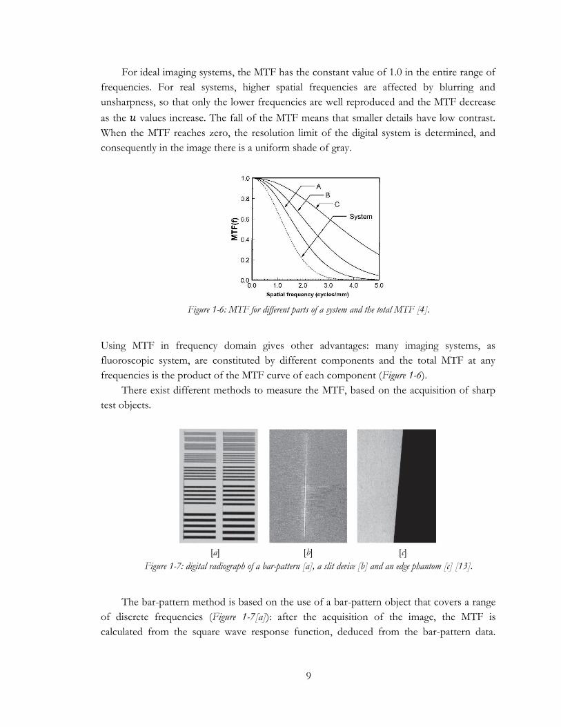
For ideal imaging systems, the MTF has the constant value of 1.0 in the entire range of

frequencies. For real systems, higher spatial frequencies are affected by blurring and

unsharpness, so that only the lower frequencies are well reproduced and the MTF decrease

as the 𝑢 values increase. The fall of the MTF means that smaller details have low contrast.

When the MTF reaches zero, the resolution limit of the digital system is determined, and

consequently in the image there is a uniform shade of gray.

Figure 1-6: MTF for different parts of a system and the total MTF [4].

Using MTF in frequency domain gives other advantages: many imaging systems, as

fluoroscopic system, are constituted by different components and the total MTF at any

frequencies is the product of the MTF curve of each component (Figure 1-6).

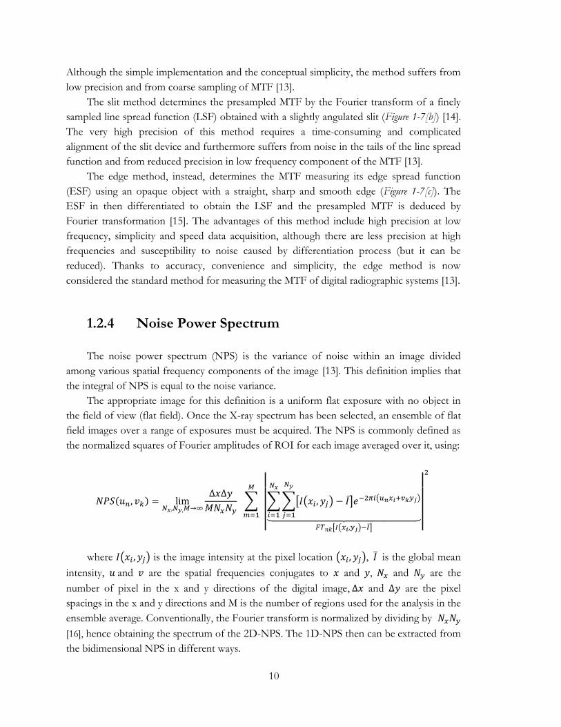
There exist different methods to measure the MTF, based on the acquisition of sharp

test objects.

[a] [b] [c]

Figure 1-7: digital radiograph of a bar-pattern [a], a slit device [b] and an edge phantom [c] [13].

The bar-pattern method is based on the use of a bar-pattern object that covers a range

of discrete frequencies (Figure 1-7[a]): after the acquisition of the image, the MTF is

calculated from the square wave response function, deduced from the bar-pattern data.

10

Although the simple implementation and the conceptual simplicity, the method suffers from

low precision and from coarse sampling of MTF [13].

The slit method determines the presampled MTF by the Fourier transform of a finely

sampled line spread function (LSF) obtained with a slightly angulated slit (Figure 1-7[b]) [14].

The very high precision of this method requires a time-consuming and complicated

alignment of the slit device and furthermore suffers from noise in the tails of the line spread

function and from reduced precision in low frequency component of the MTF [13].

The edge method, instead, determines the MTF measuring its edge spread function

(ESF) using an opaque object with a straight, sharp and smooth edge (Figure 1-7[c]). The

ESF in then differentiated to obtain the LSF and the presampled MTF is deduced by

Fourier transformation [15]. The advantages of this method include high precision at low

frequency, simplicity and speed data acquisition, although there are less precision at high

frequencies and susceptibility to noise caused by differentiation process (but it can be

reduced). Thanks to accuracy, convenience and simplicity, the edge method is now

considered the standard method for measuring the MTF of digital radiographic systems [13].

1.2.4 Noise Power Spectrum

The noise power spectrum (NPS) is the variance of noise within an image divided

among various spatial frequency components of the image [13]. This definition implies that

the integral of NPS is equal to the noise variance.

The appropriate image for this definition is a uniform flat exposure with no object in

the field of view (flat field). Once the X-ray spectrum has been selected, an ensemble of flat

field images over a range of exposures must be acquired. The NPS is commonly defined as

the normalized squares of Fourier amplitudes of ROI for each image averaged over it, using:

𝑁𝑃𝑆(𝑢𝑛, 𝑣𝑘) = lim𝑁𝑥,𝑁𝑦,𝑀→∞

∆𝑥∆𝑦

𝑀𝑁𝑥𝑁𝑦 ∑

|

|∑∑[𝐼(𝑥𝑖, 𝑦𝑗) − 𝐼]𝑒

−2𝜋𝑖(𝑢𝑛𝑥𝑖+𝑣𝑘𝑦𝑗)

𝑁𝑦

𝑗=1

𝑁𝑥

𝑖=1⏟ 𝐹𝑇𝑛𝑘[𝐼(𝑥𝑖,𝑦𝑗)−𝐼]

|

|

2

𝑀

𝑚=1

where 𝐼(𝑥𝑖 , 𝑦𝑗) is the image intensity at the pixel location (𝑥𝑖, 𝑦𝑗), 𝐼 is the global mean

intensity, 𝑢 and 𝑣 are the spatial frequencies conjugates to 𝑥 and 𝑦, 𝑁𝑥 and 𝑁𝑦 are the

number of pixel in the x and y directions of the digital image, ∆𝑥 and ∆𝑦 are the pixel

spacings in the x and y directions and M is the number of regions used for the analysis in the

ensemble average. Conventionally, the Fourier transform is normalized by dividing by 𝑁𝑥𝑁𝑦

[16], hence obtaining the spectrum of the 2D-NPS. The 1D-NPS then can be extracted from

the bidimensional NPS in different ways.

11

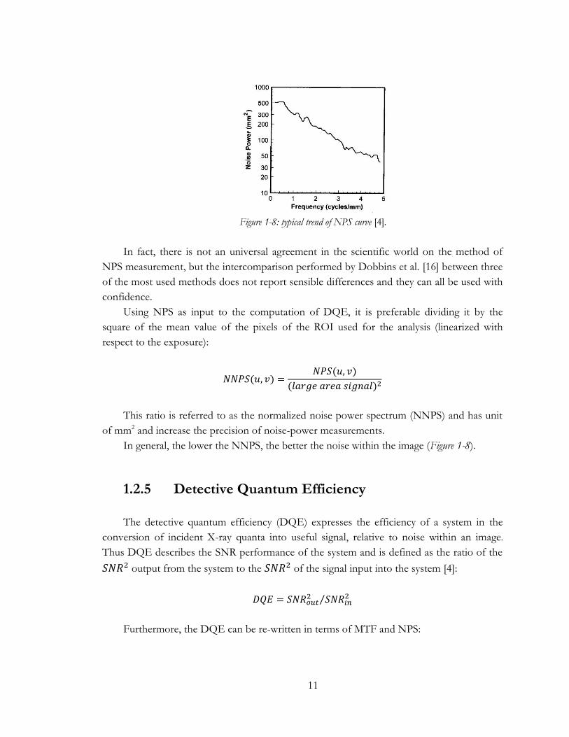
Figure 1-8: typical trend of NPS curve [4].

In fact, there is not an universal agreement in the scientific world on the method of

NPS measurement, but the intercomparison performed by Dobbins et al. [16] between three

of the most used methods does not report sensible differences and they can all be used with

confidence.

Using NPS as input to the computation of DQE, it is preferable dividing it by the

square of the mean value of the pixels of the ROI used for the analysis (linearized with

respect to the exposure):

𝑁𝑁𝑃𝑆(𝑢, 𝑣) =𝑁𝑃𝑆(𝑢, 𝑣)

(𝑙𝑎𝑟𝑔𝑒 𝑎𝑟𝑒𝑎 𝑠𝑖𝑔𝑛𝑎𝑙)2

This ratio is referred to as the normalized noise power spectrum (NNPS) and has unit

of mm2 and increase the precision of noise-power measurements.

In general, the lower the NNPS, the better the noise within the image (Figure 1-8).

1.2.5 Detective Quantum Efficiency

The detective quantum efficiency (DQE) expresses the efficiency of a system in the

conversion of incident X-ray quanta into useful signal, relative to noise within an image.

Thus DQE describes the SNR performance of the system and is defined as the ratio of the

𝑆𝑁𝑅2 output from the system to the 𝑆𝑁𝑅2 of the signal input into the system [4]:

𝐷𝑄𝐸 = 𝑆𝑁𝑅𝑜𝑢𝑡2 𝑆𝑁𝑅𝑖𝑛

2⁄

Furthermore, the DQE can be re-written in terms of MTF and NPS:

12

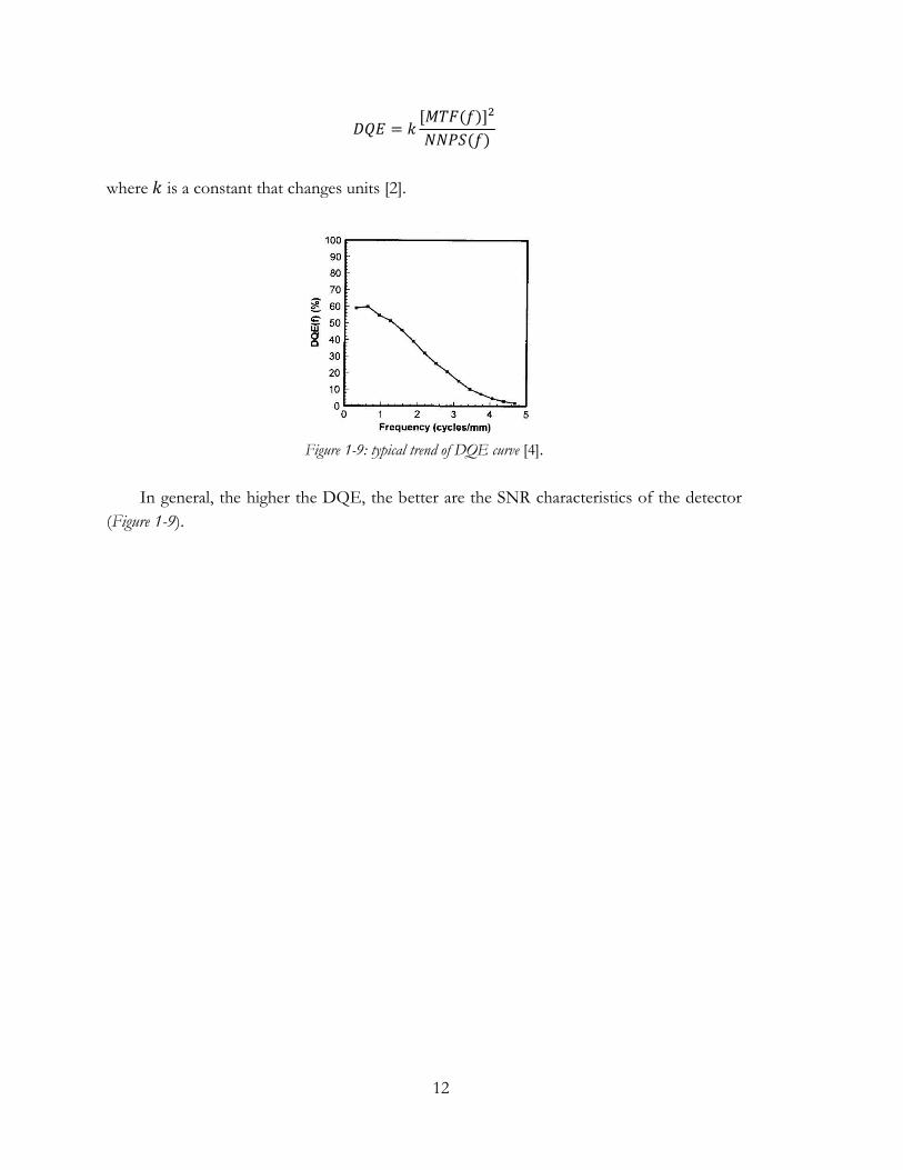
𝐷𝑄𝐸 = 𝑘[𝑀𝑇𝐹(𝑓)]2

𝑁𝑁𝑃𝑆(𝑓)

where 𝑘 is a constant that changes units [2].

Figure 1-9: typical trend of DQE curve [4].

In general, the higher the DQE, the better are the SNR characteristics of the detector

(Figure 1-9).

13

Chapter 2 Materials and methods

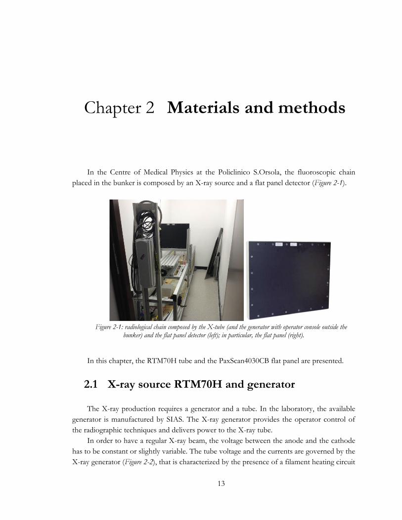
In the Centre of Medical Physics at the Policlinico S.Orsola, the fluoroscopic chain

placed in the bunker is composed by an X-ray source and a flat panel detector (Figure 2-1).

Figure 2-1: radiological chain composed by the X-tube (and the generator with operator console outside the

bunker) and the flat panel detector (left); in particular, the flat panel (right).

In this chapter, the RTM70H tube and the PaxScan4030CB flat panel are presented.

2.1 X-ray source RTM70H and generator

The X-ray production requires a generator and a tube. In the laboratory, the available

generator is manufactured by SIAS. The X-ray generator provides the operator control of

the radiographic techniques and delivers power to the X-ray tube.

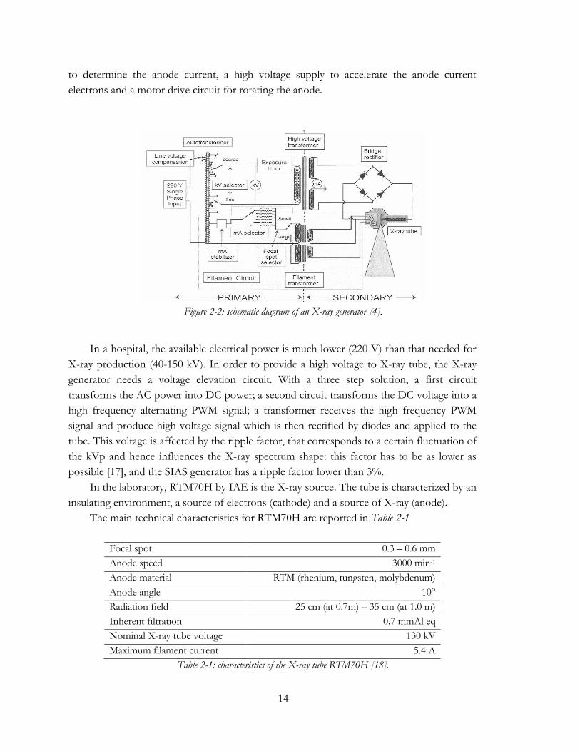
In order to have a regular X-ray beam, the voltage between the anode and the cathode

has to be constant or slightly variable. The tube voltage and the currents are governed by the

X-ray generator (Figure 2-2), that is characterized by the presence of a filament heating circuit

14

to determine the anode current, a high voltage supply to accelerate the anode current

electrons and a motor drive circuit for rotating the anode.

Figure 2-2: schematic diagram of an X-ray generator [4].

In a hospital, the available electrical power is much lower (220 V) than that needed for

X-ray production (40-150 kV). In order to provide a high voltage to X-ray tube, the X-ray

generator needs a voltage elevation circuit. With a three step solution, a first circuit

transforms the AC power into DC power; a second circuit transforms the DC voltage into a

high frequency alternating PWM signal; a transformer receives the high frequency PWM

signal and produce high voltage signal which is then rectified by diodes and applied to the

tube. This voltage is affected by the ripple factor, that corresponds to a certain fluctuation of

the kVp and hence influences the X-ray spectrum shape: this factor has to be as lower as

possible [17], and the SIAS generator has a ripple factor lower than 3%.

In the laboratory, RTM70H by IAE is the X-ray source. The tube is characterized by an

insulating environment, a source of electrons (cathode) and a source of X-ray (anode).

The main technical characteristics for RTM70H are reported in Table 2-1

Focal spot 0.3 – 0.6 mm

Anode speed 3000 min-1

Anode material RTM (rhenium, tungsten, molybdenum)

Anode angle 10°

Radiation field 25 cm (at 0.7m) – 35 cm (at 1.0 m)

Inherent filtration 0.7 mmAl eq

Nominal X-ray tube voltage 130 kV

Maximum filament current 5.4 A

Table 2-1: characteristics of the X-ray tube RTM70H [18].

15

In medical imaging, the typical range of tube voltages is 40-150 kV for general

diagnostic radiology and 25-40 kV for mammography. The RTM70H reaches 130kV

nominal tube voltage.

In RTM70H, the cathode filament is composed by tungsten and is heated by a current

that reaches the maximum value of 5.4 A. The filament current directly influences the tube,

or anodic, current (mA): the electrons emitted by the filament move toward the anode,

following the electric field determined by the voltage (kVp) between anode and cathode. In

general, at any kV, the X-ray flux is proportional to the tube current.

The operator cannot select the filament current, but on the other hand it is possible

setting many other parameters from the generator console, as the tube voltage, the tube

current, the exposure time and so on. The selection of the mA usually determines the size of

the focal spot and the RTM70H performs different cathode emission depending on it. The

presence of two filaments gives two different focal spot: the smaller focal spot (0.3) is

suitable for fluoroscopic procedures, that requires detailed images, and the bigger focal spot

(0.6) is adapt to radiography, characterized by high photon fluence and high power.

The anode in an X-ray tube principally perform two uses: the former, obviously, is the

production of the X-ray beam, the second is the management of the heat generated during

the process. The technological development leads from the stationary anode to the rotating

anode: in RTM70H, the anode track is made of tungsten while the plate is composed with

parts of rhenium and molybdenum, and its speed is of 3000/min. In such manner, the

anode is heated by the electronic beam only for the interval necessary to match the focal

spot, while during the remaining rotation heat is ceased to a larger surface.

All the energy incident on the anode amasses in the anode material: the heat produced

depends on kVp, mA and exposure time and its dissipation should be as better as possible

to prevent the anode rupture. All these quantities can be measured in thermal units (HU).

The maximum heat content is the maximum energy that anode can amount reaching its

maximum allowable temperature.

2.2 Flat panel PaxScan 4030CB Varian

The PaxScan 4030CB designed and manufactured by Varian Medical Systems is a

digital X-ray flat panel imager. This imager replaces image intensifiers and TV cameras in

fluoroscopic X-ray procedures: one of its main characteristics is the possibility of program

the frame rate, sensitivity, field-of-view and resolution in order to obtain many read out

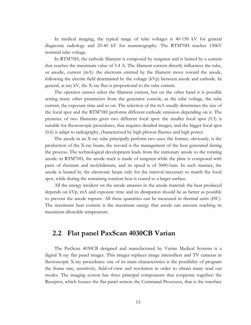
modes. The imaging system has three principal components that cooperate together: the

Receptor, which houses the flat panel sensor; the Command Processor, that is the interface

16

between the Receptor and the imaging system; the Power Supply that provides all the DC

power necessary for both the Command Processor and the Receptor (Figure 2-3).

.

Figure 2-3: PaxScan Imager configuration [19].

Typically, the Command Processor and the Power Supply are mounted in an

equipment enclosures and are not in view or reach of the patient or the operator.

2.2.1 The scintillator

The internal configuration of the Receptor in made up by the X-ray scintillator, a

Thallium-doped Cesium Iodide (CsI(Tl)) deposited directly on the amorphous silicon (a-Si)

array and with a thickness of 600 µm. The main technical characteristics of the PaxScan

4030CB are reported in Table 2-2.

Cesium and iodine have high atomic numbers (ZC=55 and ZI=53, respectively) and

hence have good X-ray absorption properties. They also exhibit an increase in X-ray

absorption at photon energies that exceed their K-egde (36 keV for cesium and 33 keV for

iodine), ensuring an efficient absorption of X-ray photons in the energy range relevant for

fluoroscopy and fluorography. In flat panel detectors, the cesium iodide layers are

exclusively doped with Tl because, compared to the sodium(Na)-doped CsI used in the

image intensifiers, they are less hygroscopic and the emission spectrum (green) is better

matched to the spectral sensitivity of the a-Si photodiodes [20].

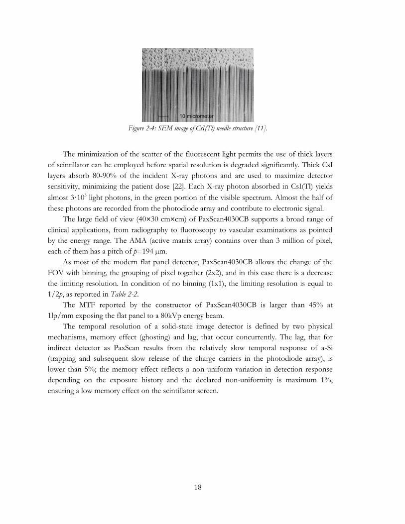
The CsI(Tl) scintillator is deposited in a columnar structure (Figure 2-4) that acts as a

light guide, suppressing the lateral light diffusion and reducing the degradation of spatial

resolution. The columnar structure also guarantees a high packing density (90%),

contributing to maximize X-ray absorption. It has been measured that, for a given thickness

of scintillator, the CsI(Tl) layers maintain significantly higher resolution than powder screens

[2].

17

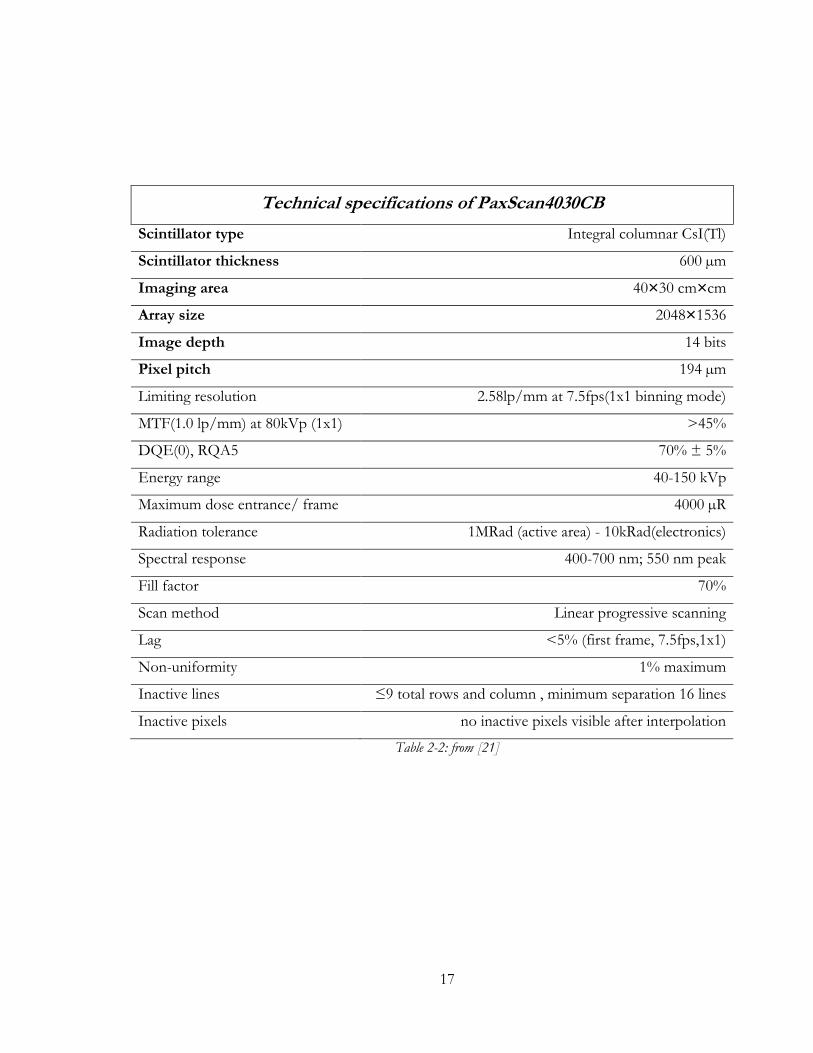
Technical specifications of PaxScan4030CB

Scintillator type Integral columnar CsI(Tl)

Scintillator thickness 600 µm

Imaging area 40×30 cm×cm

Array size 2048×1536

Image depth 14 bits

Pixel pitch 194 µm

Limiting resolution 2.58lp/mm at 7.5fps(1x1 binning mode)

MTF(1.0 lp/mm) at 80kVp (1x1) >45%

DQE(0), RQA5 70% ± 5%

Energy range 40-150 kVp

Maximum dose entrance/ frame 4000 µR

Radiation tolerance 1MRad (active area) - 10kRad(electronics)

Spectral response 400-700 nm; 550 nm peak

Fill factor 70%

Scan method Linear progressive scanning

Lag <5% (first frame, 7.5fps,1x1)

Non-uniformity 1% maximum

Inactive lines ≤9 total rows and column , minimum separation 16 lines

Inactive pixels no inactive pixels visible after interpolation

Table 2-2: from [21]

18

Figure 2-4: SEM image of CsI(Tl) needle structure [11].

The minimization of the scatter of the fluorescent light permits the use of thick layers

of scintillator can be employed before spatial resolution is degraded significantly. Thick CsI

layers absorb 80-90% of the incident X-ray photons and are used to maximize detector

sensitivity, minimizing the patient dose [22]. Each X-ray photon absorbed in CsI(Tl) yields

almost 3·103 light photons, in the green portion of the visible spectrum. Almost the half of

these photons are recorded from the photodiode array and contribute to electronic signal.

The large field of view (40×30 cm×cm) of PaxScan4030CB supports a broad range of

clinical applications, from radiography to fluoroscopy to vascular examinations as pointed

by the energy range. The AMA (active matrix array) contains over than 3 million of pixel,

each of them has a pitch of p=194 µm.

As most of the modern flat panel detector, PaxScan4030CB allows the change of the

FOV with binning, the grouping of pixel together (2x2), and in this case there is a decrease

the limiting resolution. In condition of no binning (1x1), the limiting resolution is equal to

1/2p, as reported in Table 2-2.

The MTF reported by the constructor of PaxScan4030CB is larger than 45% at

1lp/mm exposing the flat panel to a 80kVp energy beam.

The temporal resolution of a solid-state image detector is defined by two physical

mechanisms, memory effect (ghosting) and lag, that occur concurrently. The lag, that for

indirect detector as PaxScan results from the relatively slow temporal response of a-Si

(trapping and subsequent slow release of the charge carriers in the photodiode array), is

lower than 5%; the memory effect reflects a non-uniform variation in detection response

depending on the exposure history and the declared non-uniformity is maximum 1%,

ensuring a low memory effect on the scintillator screen.

19

2.2.2 Receptor, Command Processor and Power

Supply

The function of the Receptor is to absorb the X-ray beam passing through the patient,

and to convert those X-rays into a digital image. This part of the imager can be located up to

40 meters from the Command Processor: in fact, these elements are connected by a bi-

directional fiber optic link, used to pass all data and mode control signals to the Receptor,

and by a copper cable with quick disconnect connectors that provides 24V/3A for the

Receptor. The Receptor is typically mounted into structure such as a C-arm and is

completely covered by the mounting and the contrast enhancement screen. Although the

Receptor’s input window is located on the opposite side of the patient and the X-ray source,

it is possible that Receptor could inadvertently contact the patient: this closeness, not

allowed for any part of the PaxScan 4030CB, depends on the operator’s skills and the

technique being performed.

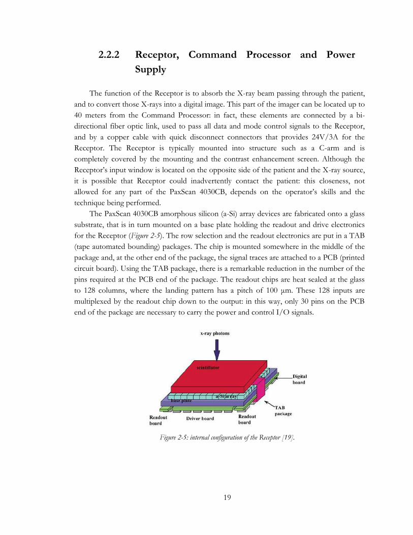
The PaxScan 4030CB amorphous silicon (a-Si) array devices are fabricated onto a glass

substrate, that is in turn mounted on a base plate holding the readout and drive electronics

for the Receptor (Figure 2-5). The row selection and the readout electronics are put in a TAB

(tape automated bounding) packages. The chip is mounted somewhere in the middle of the

package and, at the other end of the package, the signal traces are attached to a PCB (printed

circuit board). Using the TAB package, there is a remarkable reduction in the number of the

pins required at the PCB end of the package. The readout chips are heat sealed at the glass

to 128 columns, where the landing pattern has a pitch of 100 μm. These 128 inputs are

multiplexed by the readout chip down to the output: in this way, only 30 pins on the PCB

end of the package are necessary to carry the power and control I/O signals.

Figure 2-5: internal configuration of the Receptor [19].

20

The top and bottom halves of the Si-array are read in parallel, a single row at a time

progressively. The splitting of the data lines and the two sided readout electronics enable the

parallel scanning feature of the PaxScan 4030CB.

The Command Processor provides all hardware and software interfaces for

PaxScan4030CB. It consists of an embedded computer, image correction hardware and

external hardware interface connections. The Command Processor receives commands over

the Serial or Ethernet ports, configures the imager for the appropriate operating mode and

responds to hardware I/O signals. The Command Processor has a primary output that is

corrected 16-bit digital video; the allowed corrections are for off-set and gain variations and

for dead pixels and lines. In addition, the Command Processor provide a recursive filter to

smooth frame-to-frame noise. The calibration procedures of Offset and Gain variations are

performed by the IPU (Image Processing Unit) in the Command Processor FPGA. It is

then necessary for this non-uniformity compensation to have prior a Gain reference image

and a Offset reference image in the Command Processor memory.

The Power Supply connection matches to any standard wall outlet and is connected to

the Command Processor through a 50-pin D sub-miniature connector. The internal power

supply provides a 24 supply for the Receptor, and the corresponding current draw is

typically 3A.

2.2.3 The corrections

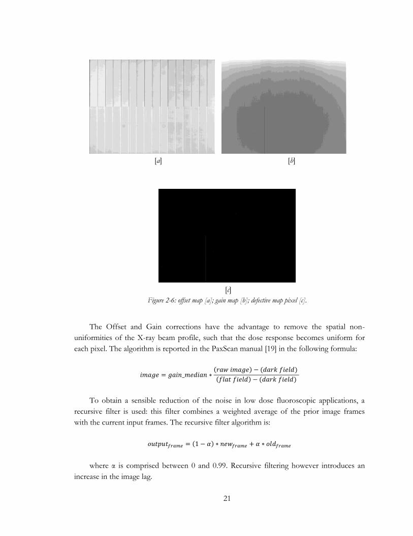
The Offset calibration corrects the fixed pattern pixel intensity variations in the image,

associated with the dark current of the Receptor and the electronic offsets introduced by the

read-out electronic. The Offset reference image comes from the average of a series of

frames acquired with no illumination (dark field). An example of Offset map can be seen in

Figure 2-6[a]. The acquisitions for the Offset calibration should commence at least 20

seconds after the X-ray exposure because of some inherent lag in the detector.

The Gain calibration is necessary to compensate for non-uniformities in the Receptor,

due to the intrinsic differences between readout amplifiers, and needs a gain reference image

(flat field) used by the IPU to correct all images in real-time. This reference image is

captured prior other images acquisition and stored in non-volatile memory, and then is

applied to all the images passing through the IPU. The Gain calibration is based upon the

linear response of the Receptor to dose and will fail with the pixels that respond in a non-

linear manner (saturation of the Receptor or low signal-to-noise ratio). To reduce the effect

of noise, the value of each pixel in the flat field image is calculated by the average of the

number of acquired frames. Then, the larger the number of calibration frames for the flat

field, the more precise the calibration will be. An example of gain map is reported in Figure

2-6[b].

21

[a] [b]

[c]

Figure 2-6: offset map [a]; gain map [b]; defective map pixel [c].

The Offset and Gain corrections have the advantage to remove the spatial non-

uniformities of the X-ray beam profile, such that the dose response becomes uniform for

each pixel. The algorithm is reported in the PaxScan manual [19] in the following formula:

𝑖𝑚𝑎𝑔𝑒 = 𝑔𝑎𝑖𝑛_𝑚𝑒𝑑𝑖𝑎𝑛 ∗(𝑟𝑎𝑤 𝑖𝑚𝑎𝑔𝑒) − (𝑑𝑎𝑟𝑘 𝑓𝑖𝑒𝑙𝑑)

(𝑓𝑙𝑎𝑡 𝑓𝑖𝑒𝑙𝑑) − (𝑑𝑎𝑟𝑘 𝑓𝑖𝑒𝑙𝑑)

To obtain a sensible reduction of the noise in low dose fluoroscopic applications, a

recursive filter is used: this filter combines a weighted average of the prior image frames

with the current input frames. The recursive filter algorithm is:

𝑜𝑢𝑡𝑝𝑢𝑡𝑓𝑟𝑎𝑚𝑒 = (1 − 𝛼) ∗ 𝑛𝑒𝑤𝑓𝑟𝑎𝑚𝑒 + 𝛼 ∗ 𝑜𝑙𝑑𝑓𝑟𝑎𝑚𝑒

where α is comprised between 0 and 0.99. Recursive filtering however introduces an

increase in the image lag.

22

Once the detector reaches the saturation level, the implemented Offset and Gain

calibrations will fail since the response to the increasing dose is not linear. To minimize

saturation effect in image with large straight-through radiation, it can be choose an

appropriate LUT for the display, otherwise there is a saturation thresholding function at the

input of the image processing section that set pixels above a certain threshold value .

The Defective pixel map is reconstructed with information from both the Offset and

the Gain reference images. The pixel correction algorithm uses nearest neighbor averaging

to replace all the defective pixels in the image. The defect map is a combination of two map:

the first is determined by the constructor and does not change, while the second is

determined during each Gain calibration. An example of detective map is observed in Figure

2-6[c]. After the correction, no defective pixels should be visible in Flat Field images.

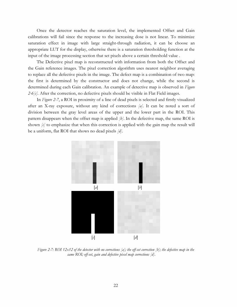
In Figure 2-7, a ROI in proximity of a line of dead pixels is selected and firstly visualized

after an X-ray exposure, without any kind of corrections [a]. It can be noted a sort of

division between the gray level areas of the upper and the lower part in the ROI. This

pattern disappears when the offset map is applied [b]. In the defective map, the same ROI is

shown [c] to emphasize that when this correction is applied with the gain map the result will

be a uniform, flat ROI that shows no dead pixels [d].

[a] [b]

[c] [d]

Figure 2-7: ROI 12x12 of the detector with no corrections [a]; the off-set correction [b]; the defective map in the same ROI; off-set, gain and defective pixel map corrections [d].

23

2.3 Algorithms of physical characterization

The evaluation of PaxScan 4030CB in terms of MTF, NNPS and DQE has been

performed with the fundamental aid of COQ, an ImageJ plugin for the physical

characterization and quality checks of digital detector [23, 24], freely available on the site

www.medphys.it/downloads.htm.

The software can deal with images coming from different modalities

(angio/fluorography, mammography, X-ray based projection radiography). To assess the

image quality of the fluoroscopic chain mounted in the laboratory, metrics such MTF and

NPS are used in the evaluation of spatial resolution and noise, and the combination of two

gives the measurement of the DQE. This software can also achieve the estimation of other

parameters inherent to the image quality control, like detector uniformity, dark and lag

analysis, and defective pixels. In general, the IEC 62220-1 standard gives the principal

guidelines in order to calculate these objective metrics [25].

MTF

In the COQ plug-in, both the edge and slit techniques for MTF evaluation are

available: for the PaxScan 4030CB characterization it has been chosen the more common

used edge method. The used phantom is a rectangular-shaped lead object with a straight

edge.

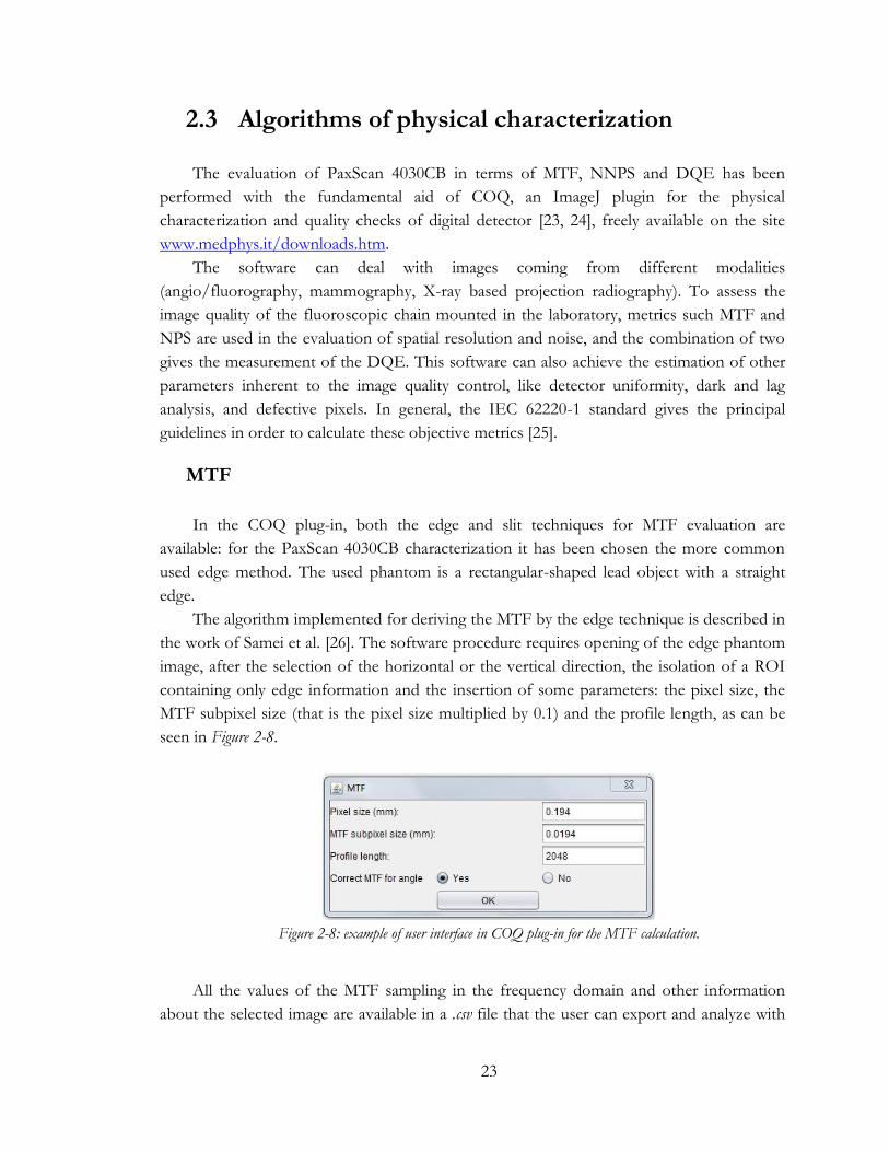
The algorithm implemented for deriving the MTF by the edge technique is described in

the work of Samei et al. [26]. The software procedure requires opening of the edge phantom

image, after the selection of the horizontal or the vertical direction, the isolation of a ROI

containing only edge information and the insertion of some parameters: the pixel size, the

MTF subpixel size (that is the pixel size multiplied by 0.1) and the profile length, as can be

seen in Figure 2-8.

Figure 2-8: example of user interface in COQ plug-in for the MTF calculation.

All the values of the MTF sampling in the frequency domain and other information

about the selected image are available in a .csv file that the user can export and analyze with

24

other software. The plot of the MTF profile can be visualized in the current result window

and can also be exported as a .txt file.

NNPS

The NNPS estimation is based on a series of flat field images acquired at the same

exposure level and opened as a stack. For a better statistics in NPS calculation, a greater

number of pixels should be considered.

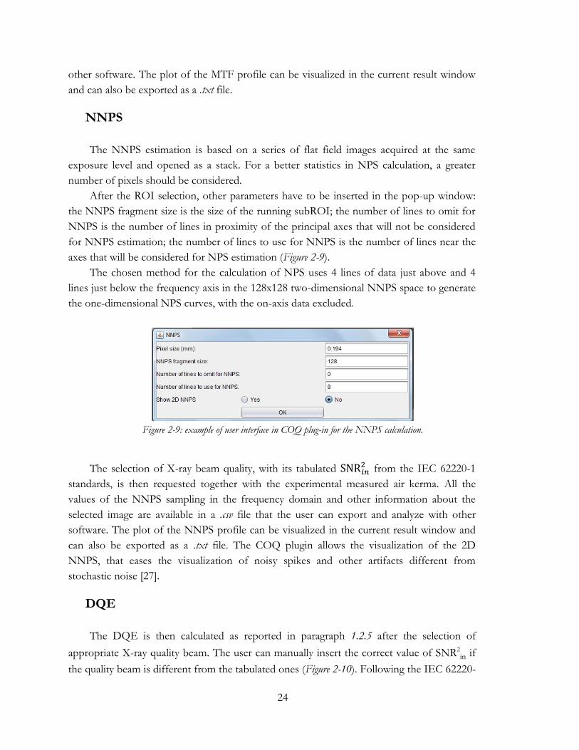
After the ROI selection, other parameters have to be inserted in the pop-up window:

the NNPS fragment size is the size of the running subROI; the number of lines to omit for

NNPS is the number of lines in proximity of the principal axes that will not be considered

for NNPS estimation; the number of lines to use for NNPS is the number of lines near the

axes that will be considered for NPS estimation (Figure 2-9).

The chosen method for the calculation of NPS uses 4 lines of data just above and 4

lines just below the frequency axis in the 128x128 two-dimensional NNPS space to generate

the one-dimensional NPS curves, with the on-axis data excluded.

Figure 2-9: example of user interface in COQ plug-in for the NNPS calculation.

The selection of X-ray beam quality, with its tabulated SNR𝑖𝑛2 from the IEC 62220-1

standards, is then requested together with the experimental measured air kerma. All the

values of the NNPS sampling in the frequency domain and other information about the

selected image are available in a .csv file that the user can export and analyze with other

software. The plot of the NNPS profile can be visualized in the current result window and

can also be exported as a .txt file. The COQ plugin allows the visualization of the 2D

NNPS, that eases the visualization of noisy spikes and other artifacts different from

stochastic noise [27].

DQE

The DQE is then calculated as reported in paragraph 1.2.5 after the selection of

appropriate X-ray quality beam. The user can manually insert the correct value of SNR2

in if

the quality beam is different from the tabulated ones (Figure 2-10). Following the IEC 62220-

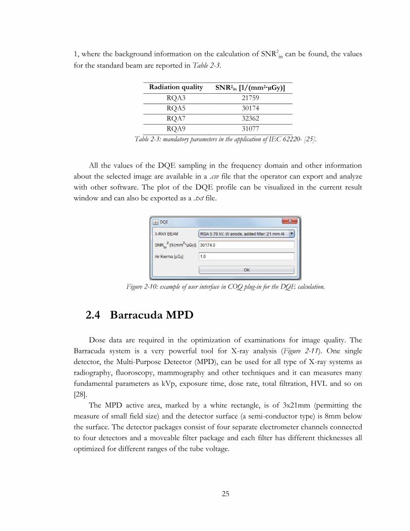
25

1, where the background information on the calculation of SNR2

in can be found, the values

for the standard beam are reported in Table 2-3.

Radiation quality SNR2in [1/(mm2·µGy)]

RQA3 21759

RQA5 30174

RQA7 32362

RQA9 31077

Table 2-3: mandatory parameters in the application of IEC 62220- [25].

All the values of the DQE sampling in the frequency domain and other information

about the selected image are available in a .csv file that the operator can export and analyze

with other software. The plot of the DQE profile can be visualized in the current result

window and can also be exported as a .txt file.

Figure 2-10: example of user interface in COQ plug-in for the DQE calculation.

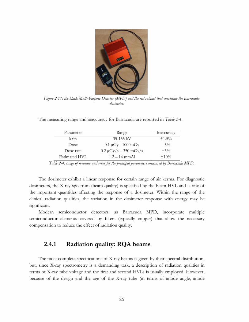
2.4 Barracuda MPD

Dose data are required in the optimization of examinations for image quality. The

Barracuda system is a very powerful tool for X-ray analysis (Figure 2-11). One single

detector, the Multi-Purpose Detector (MPD), can be used for all type of X-ray systems as

radiography, fluoroscopy, mammography and other techniques and it can measures many

fundamental parameters as kVp, exposure time, dose rate, total filtration, HVL and so on

[28].

The MPD active area, marked by a white rectangle, is of 3x21mm (permitting the

measure of small field size) and the detector surface (a semi-conductor type) is 8mm below

the surface. The detector packages consist of four separate electrometer channels connected

to four detectors and a moveable filter package and each filter has different thicknesses all

optimized for different ranges of the tube voltage.

26

Figure 2-11: the black Multi-Purpose Detector (MPD) and the red cabinet that constitute the Barracuda

dosimeter.

The measuring range and inaccuracy for Barracuda are reported in Table 2-4.

Parameter Range Inaccuracy

kVp 35-155 kV ±1.5%

Dose 0.1 µGy - 1000 µGy ±5%

Dose rate 0.2 µGy/s – 350 mGy/s ±5%

Estimated HVL 1.2 – 14 mmAl ±10%

Table 2-4: range of measure and error for the principal parameters measured by Barracuda MPD.

The dosimeter exhibit a linear response for certain range of air kerma. For diagnostic

dosimeters, the X-ray spectrum (beam quality) is specified by the beam HVL and is one of

the important quantities affecting the response of a dosimeter. Within the range of the

clinical radiation qualities, the variation in the dosimeter response with energy may be

significant.

Modern semiconductor detectors, as Barracuda MPD, incorporate multiple

semiconductor elements covered by filters (typically copper) that allow the necessary

compensation to reduce the effect of radiation quality.

2.4.1 Radiation quality: RQA beams

The most complete specifications of X-ray beams is given by their spectral distribution,

but, since X-ray spectrometry is a demanding task, a description of radiation qualities in

terms of X-ray tube voltage and the first and second HVLs is usually employed. However,

because of the design and the age of the X-ray tube (in terms of anode angle, anode

27

roughening and inherent filtration), two radiation qualities produced at a given tube voltage

having the same first HVL can still have different spectral distributions.

The standard IEC 61267 [29] deals with methods for generating radiation beams in

well-defined radiation conditions and ensures that measurements of the properties of

medical diagnostic equipment should produce consistent results if radiation qualities or

radiation conditions in compliance with the standard itself are used.

The radiation qualities of the RQA series represent simulation of the radiation field

behind the patient and they are reproduced with additional filtration of aluminum. RQA

cover the entire diagnostic energy range (from 40 up to 150 kV) and each quality, from

RQA2 to RQA10, is established by adding an aluminum filtration amounting to the sum of

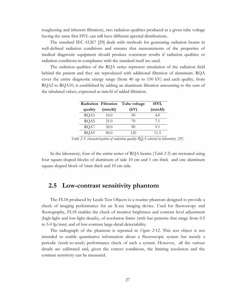
the tabulated values, expressed as mmAl of added filtration.

Radiation

quality

Filtration

(mmAl)

Tube voltage

(kV)

HVL

(mmAl)

RQA3 10.0 50 4.0

RQA5 21.0 70 7.1

RQA7 30.0 90 9.1

RQA9 40.0 120 11.5

Table 2-5: characterization of radiation quality RQA selected in laboratory [29].

In the laboratory, four of the entire series of RQA beams (Table 2-5) are recreated using

four square-shaped blocks of aluminum of side 10 cm and 1 cm thick and one aluminum

square-shaped block of 1mm thick and 10 cm side.

2.5 Low-contrast sensitivity phantom

The FL18 produced by Leeds Test Objects is a routine phantom designed to provide a

check of imaging performance for an X-ray imaging device. Used for fluoroscopy and

fluorography, FL18 enables the check of monitor brightness and contrast level adjustment

(high-light and low-light details), of resolution limits (with bar patterns that range from 0.5

to 5-0 lp/mm) and of low-contrast large-detail detectability.

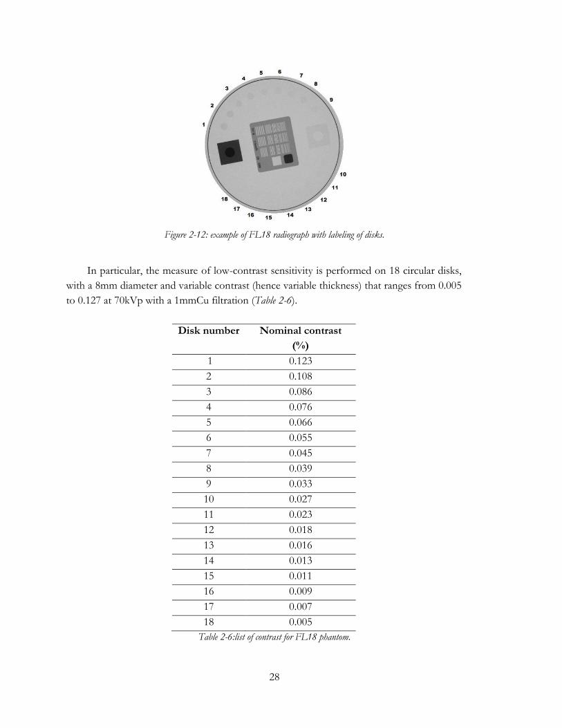
The radiograph of the phantom is reported in Figure 2-12. This test object is not

intended to enable quantitative information about a fluoroscopic system but merely a

periodic (week-to-week) performance check of such a system. However, all the various

details are calibrated and, given the correct conditions, the limiting resolution and the

contrast sensitivity can be measured.

28

Figure 2-12: example of FL18 radiograph with labeling of disks.

In particular, the measure of low-contrast sensitivity is performed on 18 circular disks,

with a 8mm diameter and variable contrast (hence variable thickness) that ranges from 0.005

to 0.127 at 70kVp with a 1mmCu filtration (Table 2-6).

Disk number Nominal contrast

(%)

1 0.123

2 0.108

3 0.086

4 0.076

5 0.066

6 0.055

7 0.045

8 0.039

9 0.033

10 0.027

11 0.023

12 0.018

13 0.016

14 0.013

15 0.011

16 0.009

17 0.007

18 0.005

Table 2-6:list of contrast for FL18 phantom.

29

Chapter 3 Results

In this chapter, the session of measures to validate and assess the fluoroscopic chain of

the laboratory is presented.

In the first place, the X-ray source RTM70H is evaluated in its ability to reproduce

RQA beams tabulated in the IEC standards. Then the main relationship with the mA and

the kVp is verified, and the efficiency at 1m is measured and compared with SpekCalc

simulation.

The PaxScan 4030CB is studied in its response curve and for each RQA beam, MTF,

NNPS and DQE – the main metrics of the image quality assessment- are calculated. All the

computations are performed with the aid of the COQ ImageJ plug-in.

3.1 RTM70H

3.1.1 Experimental establishment of RQA beams

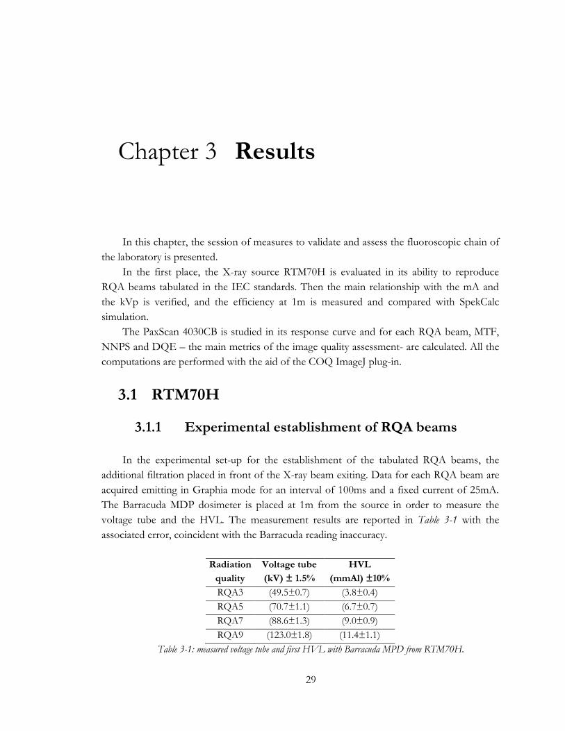
In the experimental set-up for the establishment of the tabulated RQA beams, the

additional filtration placed in front of the X-ray beam exiting. Data for each RQA beam are

acquired emitting in Graphia mode for an interval of 100ms and a fixed current of 25mA.

The Barracuda MDP dosimeter is placed at 1m from the source in order to measure the

voltage tube and the HVL. The measurement results are reported in Table 3-1 with the

associated error, coincident with the Barracuda reading inaccuracy.

Radiation

quality

Voltage tube

(kV) ± 1.5%

HVL

(mmAl) ±10%

RQA3 (49.5±0.7) (3.8±0.4)

RQA5 (70.7±1.1) (6.7±0.7)

RQA7 (88.6±1.3) (9.0±0.9)

RQA9 (123.0±1.8) (11.4±1.1)

Table 3-1: measured voltage tube and first HVL with Barracuda MPD from RTM70H.

30

The experimental RQA beams are in good agreement with the tabulated values

reported in Table 2-5, and it can be said that the RTM70H reproduces in a good way the

quality beams that will be used for the characterization of the flat panel.

3.1.2 SpekCalc simulation of RQA beams

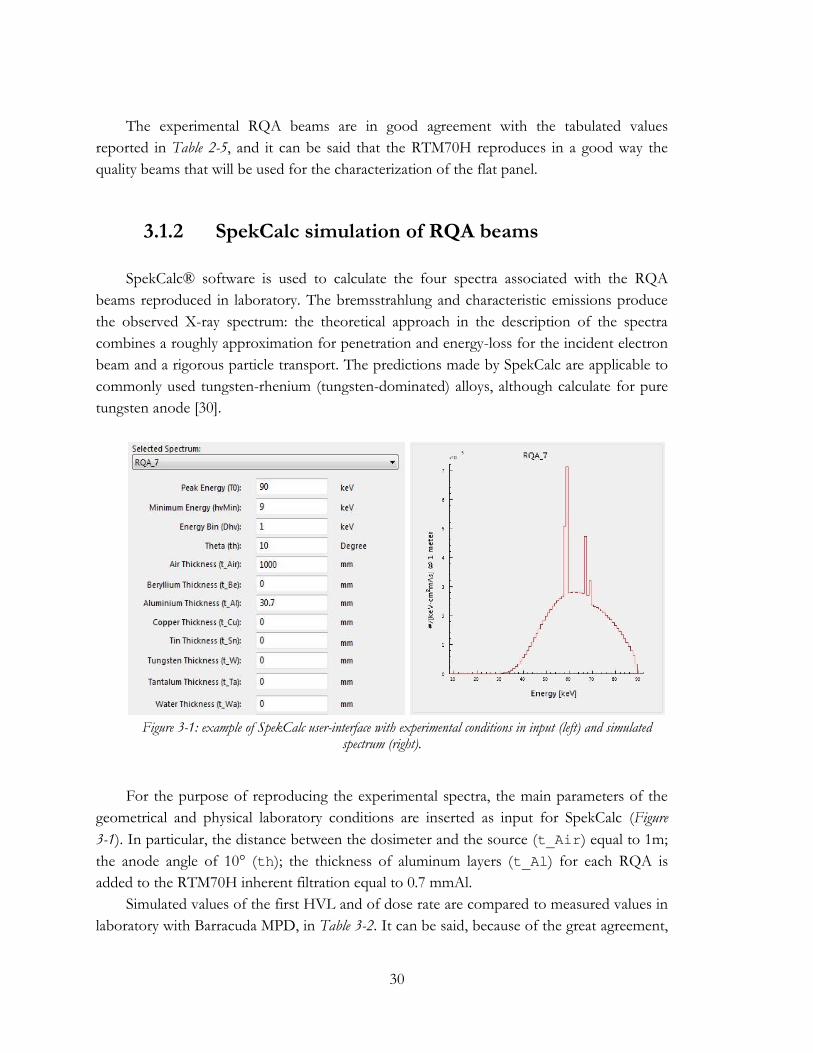
SpekCalc® software is used to calculate the four spectra associated with the RQA

beams reproduced in laboratory. The bremsstrahlung and characteristic emissions produce

the observed X-ray spectrum: the theoretical approach in the description of the spectra

combines a roughly approximation for penetration and energy-loss for the incident electron

beam and a rigorous particle transport. The predictions made by SpekCalc are applicable to

commonly used tungsten-rhenium (tungsten-dominated) alloys, although calculate for pure

tungsten anode [30].

Figure 3-1: example of SpekCalc user-interface with experimental conditions in input (left) and simulated

spectrum (right).

For the purpose of reproducing the experimental spectra, the main parameters of the

geometrical and physical laboratory conditions are inserted as input for SpekCalc (Figure

3-1). In particular, the distance between the dosimeter and the source (t_Air) equal to 1m;

the anode angle of 10° (th); the thickness of aluminum layers (t_Al) for each RQA is

added to the RTM70H inherent filtration equal to 0.7 mmAl.

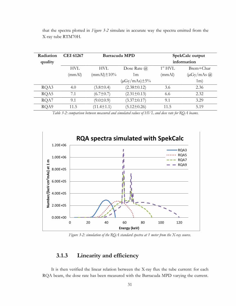
Simulated values of the first HVL and of dose rate are compared to measured values in

laboratory with Barracuda MPD, in Table 3-2. It can be said, because of the great agreement,

31

that the spectra plotted in Figure 3-2 simulate in accurate way the spectra emitted from the

X-ray tube RTM70H.

Radiation

quality

CEI 61267 Barracuda MPD SpekCalc output

information

HVL

(mmAl)

HVL

(mmAl)±10%

Dose Rate @

1m

(µGy/mAs)±5%

1st HVL

(mmAl)

Brem+Char

(µGy/mAs @

1m)

RQA3 4.0 (3.8±0.4) (2.38±0.12) 3.6 2.36

RQA5 7.1 (6.7±0.7) (2.31±0.13) 6.6 2.32

RQA7 9.1 (9.0±0.9) (3.37±0.17) 9.1 3.29

RQA9 11.5 (11.4±1.1) (5.12±0.26) 11.5 5.19

Table 3-2: comparison between measured and simulated values of HVL and dose rate for RQA beams.

Figure 3-2: simulation of the RQA standard spectra at 1 meter from the X-ray source.

3.1.3 Linearity and efficiency

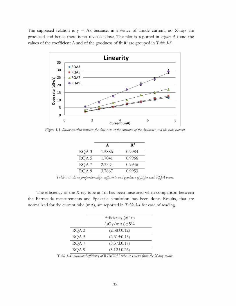
It is then verified the linear relation between the X-ray flux the tube current: for each

RQA beam, the dose rate has been measured with the Barracuda MPD varying the current.

0.00E+00

2.00E+05

4.00E+05

6.00E+05

8.00E+05

1.00E+06

1.20E+06

0 20 40 60 80 100 120

Nu

mb

er/

[ke

V·c

m2m

As]

at

1 m

Energy (keV)

RQA spectra simulated with SpekCalc

RQA3

RQA5

RQA7

RQA9

32

The supposed relation is y = Ax because, in absence of anode current, no X-rays are

produced and hence there is no revealed dose. The plot is reported in Figure 3-3 and the

values of the coefficient A and of the goodness of fit R2 are grouped in Table 3-3.

Figure 3-3: linear relation between the dose rate at the entrance of the dosimeter and the tube current.

A R2

RQA 3 1.5886 0.9984

RQA 5 1.7041 0.9966

RQA 7 2.3324 0.9946

RQA 9 3.7667 0.9953

Table 3-3: direct proportionality coefficients and goodness of fit for each RQA beam.

The efficiency of the X-ray tube at 1m has been measured when comparison between

the Barracuda measurements and Spekcalc simulation has been done. Results, that are

normalized for the current tube (mA), are reported in Table 3-4 for ease of reading.

Efficiency @ 1m

(µGy/mAs)±5%

RQA 3 (2.38±0.12)

RQA 5 (2.31±0.13)

RQA 7 (3.37±0.17)

RQA 9 (5.12±0.26)

Table 3-4: measured efficiency of RTM70H tube at 1meter from the X-ray source.

0

5

10

15

20

25

30

35

0 2 4 6 8

Do

se r

ate

(u

Gy/

s)

Current (mA)

Linearity RQA3

RQA5

RQA7

RQA9

33

3.2 Physical characterization of PaxScan 4030CB

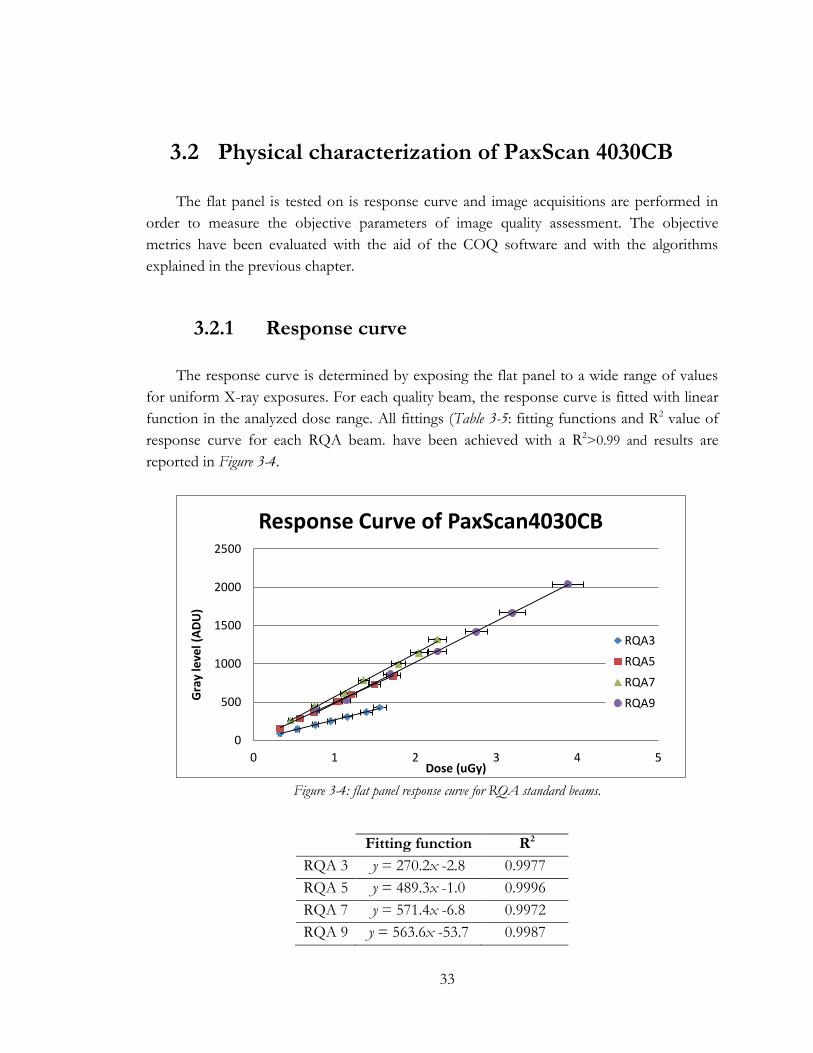
The flat panel is tested on is response curve and image acquisitions are performed in

order to measure the objective parameters of image quality assessment. The objective

metrics have been evaluated with the aid of the COQ software and with the algorithms

explained in the previous chapter.

3.2.1 Response curve

The response curve is determined by exposing the flat panel to a wide range of values

for uniform X-ray exposures. For each quality beam, the response curve is fitted with linear

function in the analyzed dose range. All fittings (Table 3-5: fitting functions and R2 value of

response curve for each RQA beam. have been achieved with a R2>0.99 and results are

reported in Figure 3-4.

Figure 3-4: flat panel response curve for RQA standard beams.

Fitting function R2

RQA 3 y = 270.2x -2.8 0.9977

RQA 5 y = 489.3x -1.0 0.9996

RQA 7 y = 571.4x -6.8 0.9972

RQA 9 y = 563.6x -53.7 0.9987

0

500

1000

1500

2000

2500

0 1 2 3 4 5

Gra

y le

vel (

AD

U)

Dose (uGy)

Response Curve of PaxScan4030CB

RQA3

RQA5

RQA7

RQA9

34

Table 3-5: fitting functions and R2 value of response curve for each RQA beam.

As reported by other authors [31, 32], the CsI scintillator presents a different response

for RQA3. This is due the different sensitivity of the detector material to the various energy

of the incoming X-ray beams. It is furthermore confirmed a peak response at RQA7 beam

but consistent with the response curves of RQA5 and RQA9: for these energies, CsI

scintillator has similar sensitivity.

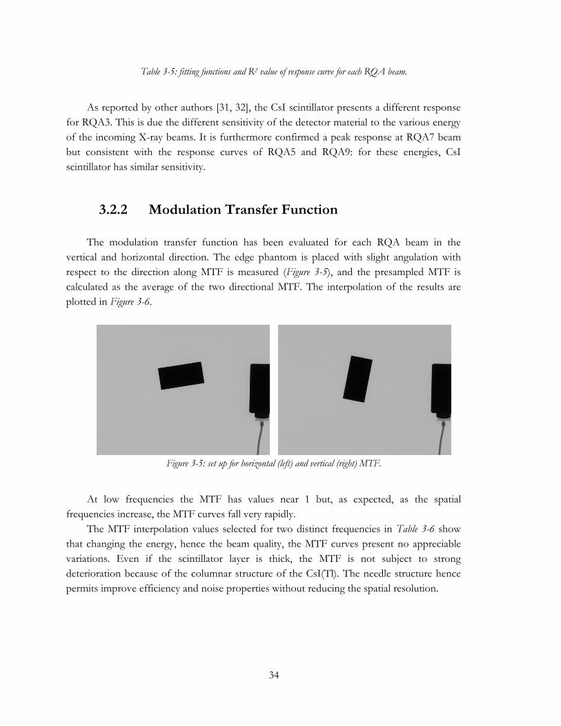
3.2.2 Modulation Transfer Function

The modulation transfer function has been evaluated for each RQA beam in the

vertical and horizontal direction. The edge phantom is placed with slight angulation with

respect to the direction along MTF is measured (Figure 3-5), and the presampled MTF is

calculated as the average of the two directional MTF. The interpolation of the results are

plotted in Figure 3-6.

Figure 3-5: set up for horizontal (left) and vertical (right) MTF.

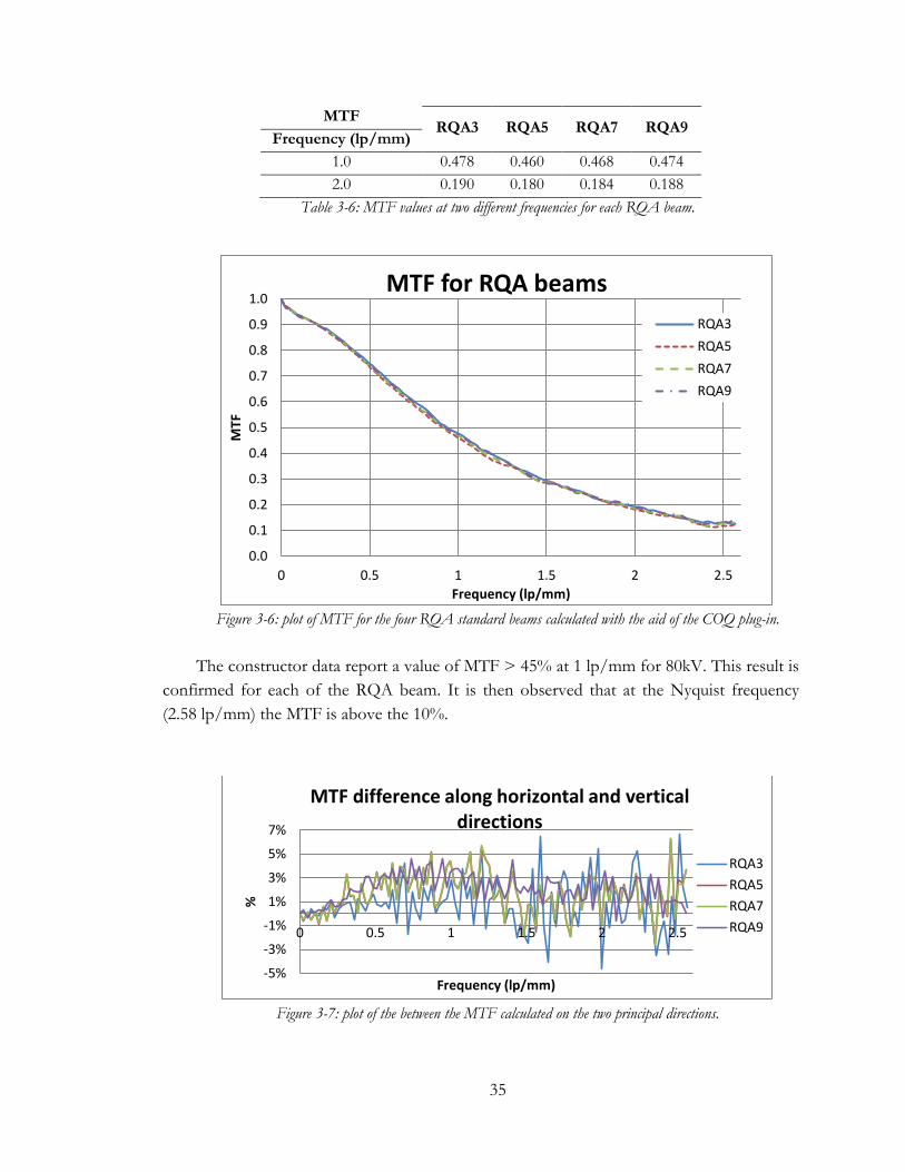
At low frequencies the MTF has values near 1 but, as expected, as the spatial

frequencies increase, the MTF curves fall very rapidly.

The MTF interpolation values selected for two distinct frequencies in Table 3-6 show

that changing the energy, hence the beam quality, the MTF curves present no appreciable

variations. Even if the scintillator layer is thick, the MTF is not subject to strong

deterioration because of the columnar structure of the CsI(Tl). The needle structure hence

permits improve efficiency and noise properties without reducing the spatial resolution.

35

MTF RQA3 RQA5 RQA7 RQA9

Frequency (lp/mm)

1.0 0.478 0.460 0.468 0.474

2.0 0.190 0.180 0.184 0.188

Table 3-6: MTF values at two different frequencies for each RQA beam.

Figure 3-6: plot of MTF for the four RQA standard beams calculated with the aid of the COQ plug-in.

The constructor data report a value of MTF > 45% at 1 lp/mm for 80kV. This result is

confirmed for each of the RQA beam. It is then observed that at the Nyquist frequency

(2.58 lp/mm) the MTF is above the 10%.

Figure 3-7: plot of the between the MTF calculated on the two principal directions.

0.0

0.1

0.2

0.3

0.4

0.5

0.6

0.7

0.8

0.9

1.0

0 0.5 1 1.5 2 2.5

MTF

Frequency (lp/mm)

MTF for RQA beams

RQA3

RQA5

RQA7

RQA9

-5%

-3%

-1%

1%

3%

5%

7%

0 0.5 1 1.5 2 2.5

%

Frequency (lp/mm)

MTF difference along horizontal and vertical directions

RQA3

RQA5

RQA7

RQA9

36

The difference between the MTF curves calculated along vertical and horizontal

directions is plotted in Figure 3-7 for each RQA beam. The small variations, around 6%,

suggest an isotropic response of the detector even if the mechanical scanning is performed

along one direction.

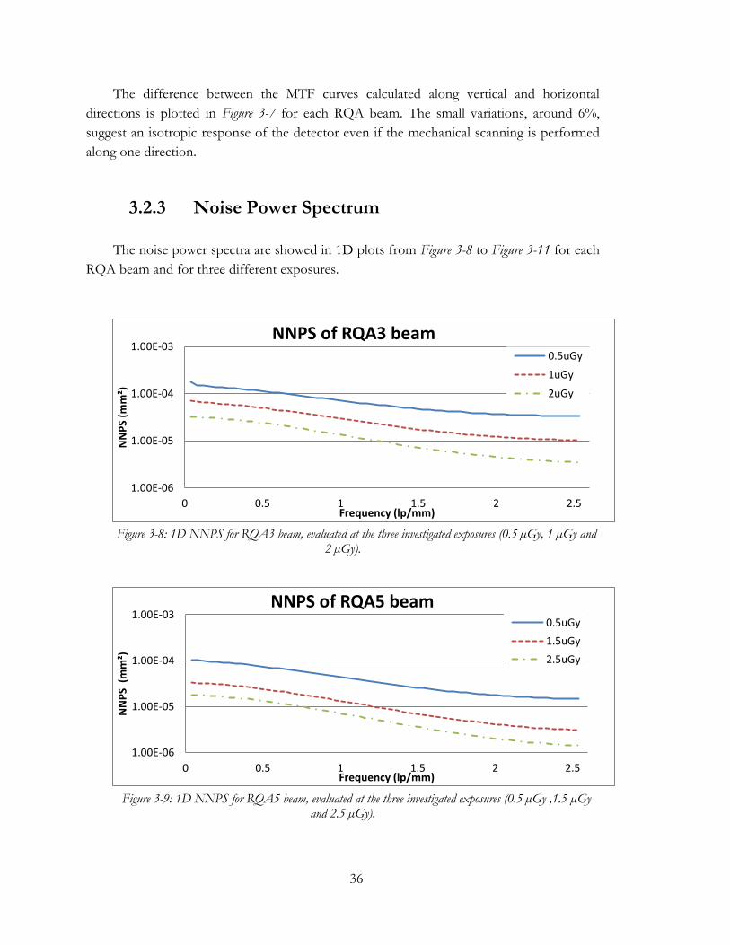
3.2.3 Noise Power Spectrum

The noise power spectra are showed in 1D plots from Figure 3-8 to Figure 3-11 for each

RQA beam and for three different exposures.

Figure 3-8: 1D NNPS for RQA3 beam, evaluated at the three investigated exposures (0.5 µGy, 1 µGy and

2 µGy).

Figure 3-9: 1D NNPS for RQA5 beam, evaluated at the three investigated exposures (0.5 µGy ,1.5 µGy

and 2.5 µGy).

1.00E-06

1.00E-05

1.00E-04

1.00E-03

0 0.5 1 1.5 2 2.5

NN

PS

(mm

²)

Frequency (lp/mm)

NNPS of RQA3 beam 0.5uGy

1uGy

2uGy

1.00E-06

1.00E-05

1.00E-04

1.00E-03

0 0.5 1 1.5 2 2.5

NN

PS

(m

m²)

Frequency (lp/mm)

NNPS of RQA5 beam 0.5uGy

1.5uGy

2.5uGy

37

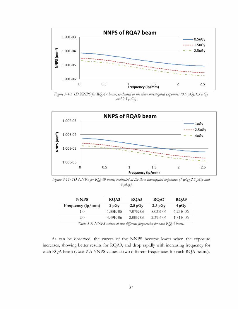
Figure 3-10: 1D NNPS for RQA7 beam, evaluated at the three investigated exposures (0.5 µGy,1.5 µGy

and 2.5 µGy).

Figure 3-11: 1D NNPS for RQA9 beam, evaluated at the three investigated exposures (1 µGy,2.5 µGy and

4 µGy).

NNPS RQA3 RQA5 RQA7 RQA9

Frequency (lp/mm) 2 µGy 2.5 µGy 2.5 µGy 4 µGy

1.0 1.33E-05 7.07E-06 8.03E-06 6.27E-06

2.0 4.49E-06 2.00E-06 2.39E-06 1.81E-06

Table 3-7: NNPS values at two different frequencies for each RQA beam.

As can be observed, the curves of the NNPS become lower when the exposure

increases, showing better results for RQA9, and drop rapidly with increasing frequency for

each RQA beam (Table 3-7: NNPS values at two different frequencies for each RQA beam.).

1.00E-06

1.00E-05

1.00E-04

1.00E-03

0 0.5 1 1.5 2 2.5

NN

PS

(mm

²)

Frequency (lp/mm)

NNPS of RQA7 beam 0.5uGy

1.5uGy

2.5uGy

1.00E-06

1.00E-05

1.00E-04

1.00E-03

0 0.5 1 1.5 2 2.5

NN

PS

(mm

²)

Frequency (lp/mm)

NNPS of RQA9 beam 1uGy

2.5uGy

4uGy

38

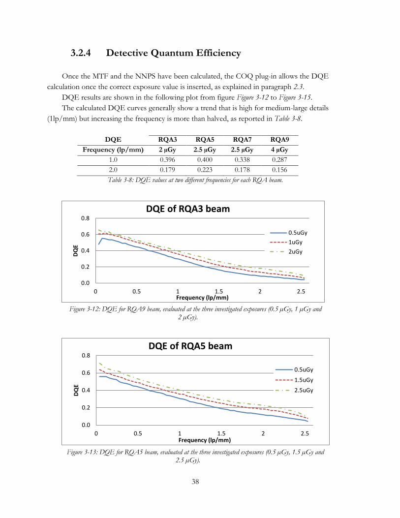
3.2.4 Detective Quantum Efficiency

Once the MTF and the NNPS have been calculated, the COQ plug-in allows the DQE

calculation once the correct exposure value is inserted, as explained in paragraph 2.3.

DQE results are shown in the following plot from figure Figure 3-12 to Figure 3-15.

The calculated DQE curves generally show a trend that is high for medium-large details

(1lp/mm) but increasing the frequency is more than halved, as reported in Table 3-8.

DQE RQA3 RQA5 RQA7 RQA9

Frequency (lp/mm) 2 µGy 2.5 µGy 2.5 µGy 4 µGy

1.0 0.396 0.400 0.338 0.287

2.0 0.179 0.223 0.178 0.156

Table 3-8: DQE values at two different frequencies for each RQA beam.

Figure 3-12: DQE for RQA9 beam, evaluated at the three investigated exposures (0.5 µGy, 1 µGy and

2 µGy).

Figure 3-13: DQE for RQA5 beam, evaluated at the three investigated exposures (0.5 µGy, 1.5 µGy and

2.5 µGy).

0.0

0.2

0.4

0.6

0.8

0 0.5 1 1.5 2 2.5

DQ

E

Frequency (lp/mm)

DQE of RQA3 beam

0.5uGy

1uGy

2uGy

0.0

0.2

0.4

0.6

0.8

0 0.5 1 1.5 2 2.5

DQ

E

Frequency (lp/mm)

DQE of RQA5 beam

0.5uGy

1.5uGy

2.5uGy

39

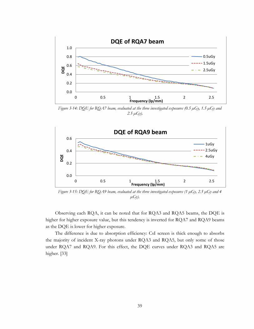
Figure 3-14: DQE for RQA7 beam, evaluated at the three investigated exposures (0.5 µGy, 1.5 µGy and

2.5 µGy).

Figure 3-15: DQE for RQA9 beam, evaluated at the three investigated exposures (1 µGy, 2.5 µGy and 4

µGy).

Observing each RQA, it can be noted that for RQA3 and RQA5 beams, the DQE is

higher for higher exposure value, but this tendency is inverted for RQA7 and RQA9 beams

as the DQE is lower for higher exposure.

The difference is due to absorption efficiency: CsI screen is thick enough to absorbs

the majority of incident X-ray photons under RQA3 and RQA5, but only some of those

under RQA7 and RQA9. For this effect, the DQE curves under RQA3 and RQA5 are

higher. [33]

0.0

0.2

0.4

0.6

0.8

1.0

0 0.5 1 1.5 2 2.5

DQ

E

Frequency (lp/mm)

DQE of RQA7 beam

0.5uGy

1.5uGy

2.5uGy

0.0

0.2

0.4

0.6

0 0.5 1 1.5 2 2.5

DQ

E

Frequency (lp/mm)

DQE of RQA9 beam

1uGy

2.5uGy

4uGy

40

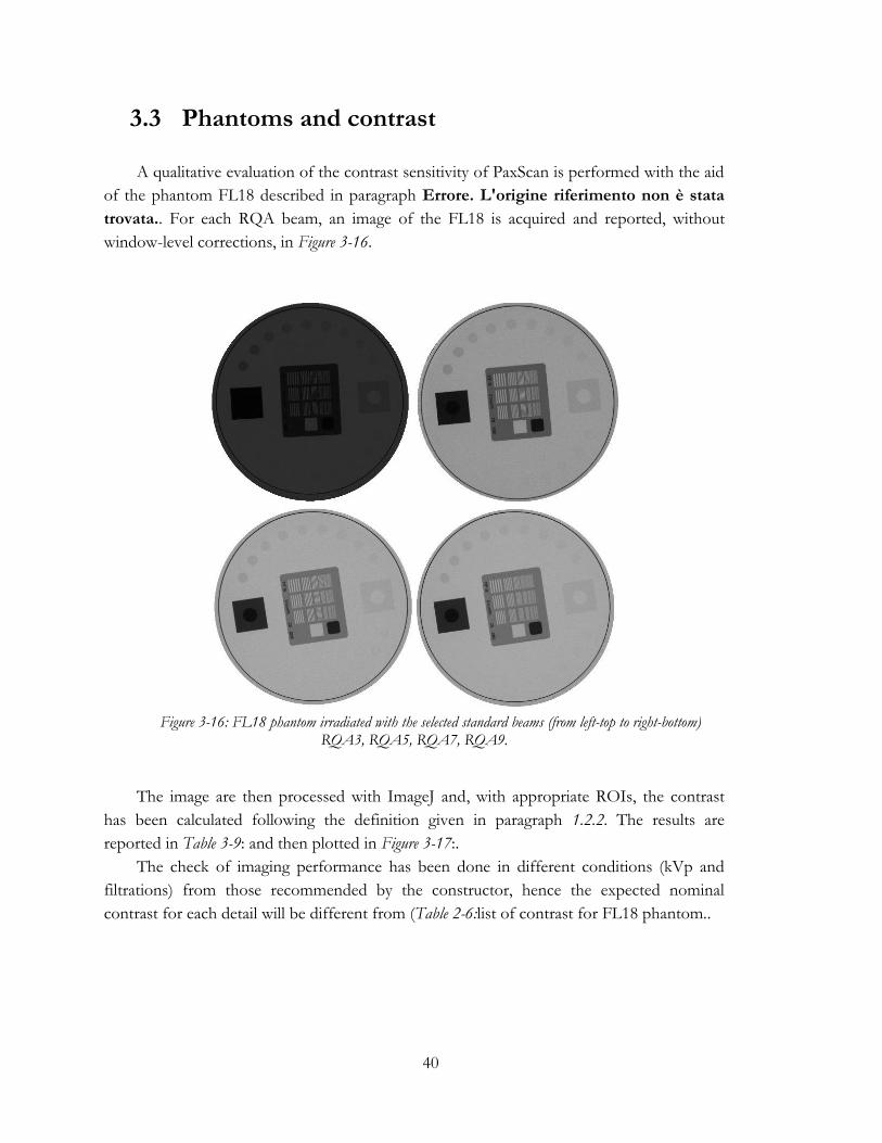
3.3 Phantoms and contrast

A qualitative evaluation of the contrast sensitivity of PaxScan is performed with the aid

of the phantom FL18 described in paragraph Errore. L'origine riferimento non è stata

trovata.. For each RQA beam, an image of the FL18 is acquired and reported, without

window-level corrections, in Figure 3-16.

Figure 3-16: FL18 phantom irradiated with the selected standard beams (from left-top to right-bottom)

RQA3, RQA5, RQA7, RQA9.

The image are then processed with ImageJ and, with appropriate ROIs, the contrast

has been calculated following the definition given in paragraph 1.2.2. The results are

reported in Table 3-9: and then plotted in Figure 3-17:.

The check of imaging performance has been done in different conditions (kVp and

filtrations) from those recommended by the constructor, hence the expected nominal

contrast for each detail will be different from (Table 2-6:list of contrast for FL18 phantom..

41

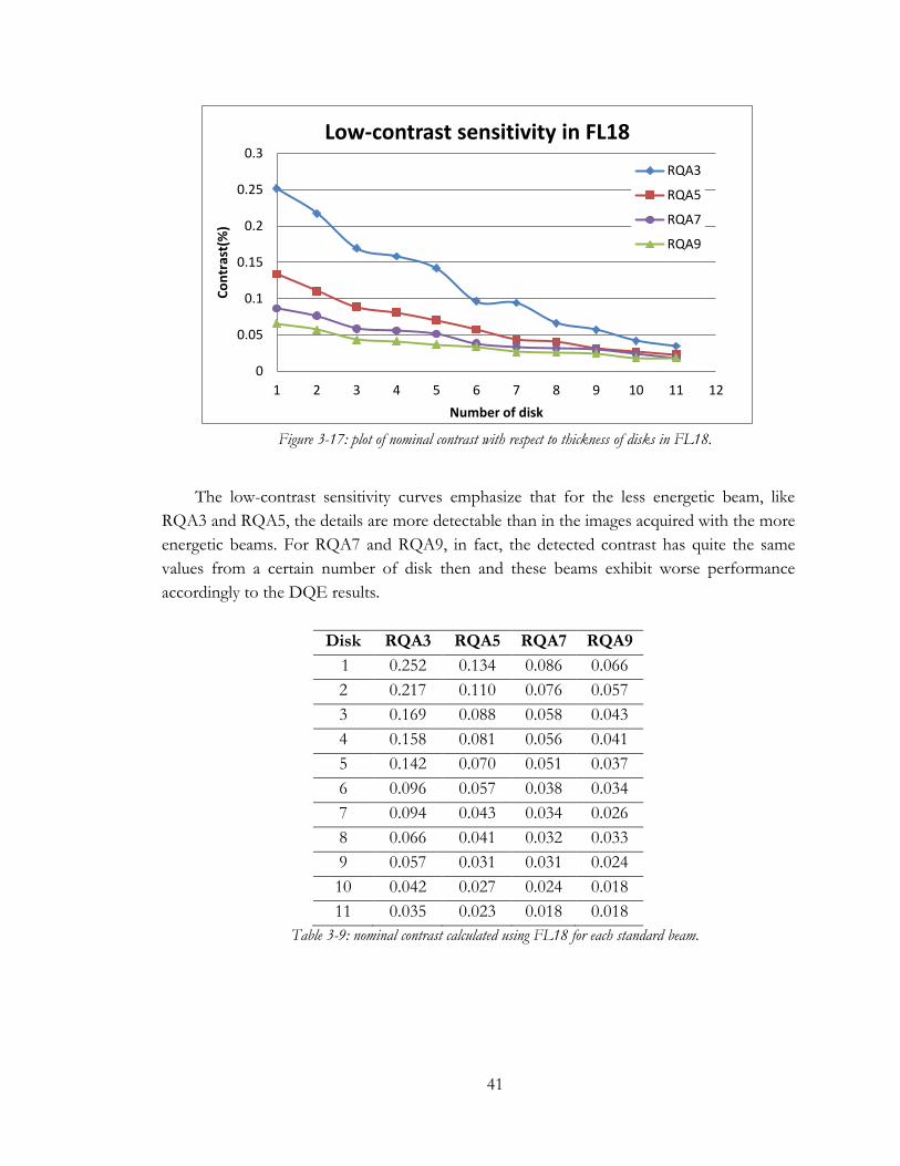
Figure 3-17: plot of nominal contrast with respect to thickness of disks in FL18.

The low-contrast sensitivity curves emphasize that for the less energetic beam, like

RQA3 and RQA5, the details are more detectable than in the images acquired with the more

energetic beams. For RQA7 and RQA9, in fact, the detected contrast has quite the same

values from a certain number of disk then and these beams exhibit worse performance

accordingly to the DQE results.

Disk RQA3 RQA5 RQA7 RQA9

1 0.252 0.134 0.086 0.066

2 0.217 0.110 0.076 0.057

3 0.169 0.088 0.058 0.043

4 0.158 0.081 0.056 0.041

5 0.142 0.070 0.051 0.037

6 0.096 0.057 0.038 0.034

7 0.094 0.043 0.034 0.026

8 0.066 0.041 0.032 0.033

9 0.057 0.031 0.031 0.024

10 0.042 0.027 0.024 0.018

11 0.035 0.023 0.018 0.018

Table 3-9: nominal contrast calculated using FL18 for each standard beam.

0

0.05

0.1

0.15

0.2

0.25

0.3

1 2 3 4 5 6 7 8 9 10 11 12

Co

ntr

ast(

%)

Number of disk

Low-contrast sensitivity in FL18

RQA3

RQA5

RQA7

RQA9

42

3.5 Flat panel detectors in literature

Flat panel imagers for digital radiography are based on direct and indirect conversion

method. After the performance evaluation of the PaxScan4030, data from other works are

reported for a general comparison of available performances for this technology.

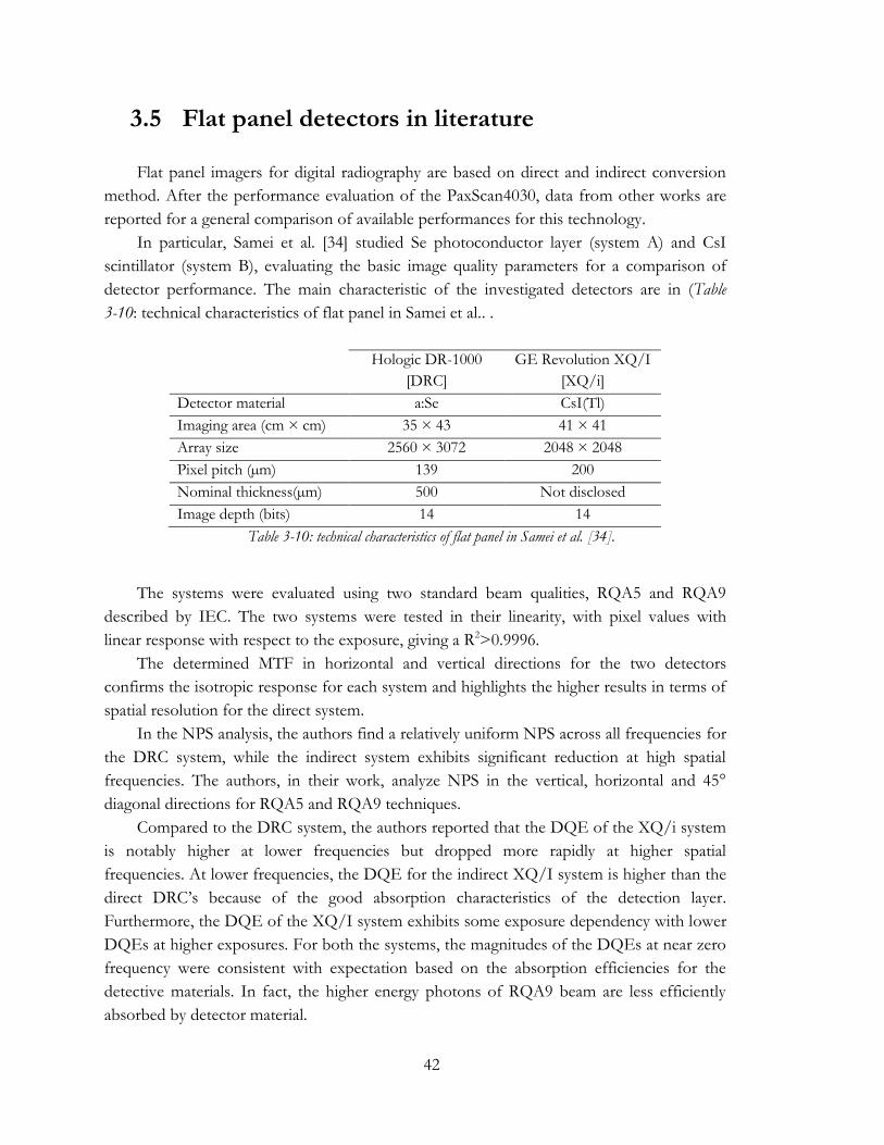
In particular, Samei et al. [34] studied Se photoconductor layer (system A) and CsI

scintillator (system B), evaluating the basic image quality parameters for a comparison of

detector performance. The main characteristic of the investigated detectors are in (Table

3-10: technical characteristics of flat panel in Samei et al.. .

Hologic DR-1000

[DRC]

GE Revolution XQ/I

[XQ/i]

Detector material a:Se CsI(Tl)

Imaging area (cm × cm) 35 × 43 41 × 41

Array size 2560 × 3072 2048 × 2048

Pixel pitch (µm) 139 200

Nominal thickness(µm) 500 Not disclosed

Image depth (bits) 14 14

Table 3-10: technical characteristics of flat panel in Samei et al. [34].

The systems were evaluated using two standard beam qualities, RQA5 and RQA9

described by IEC. The two systems were tested in their linearity, with pixel values with

linear response with respect to the exposure, giving a R2>0.9996.

The determined MTF in horizontal and vertical directions for the two detectors

confirms the isotropic response for each system and highlights the higher results in terms of

spatial resolution for the direct system.

In the NPS analysis, the authors find a relatively uniform NPS across all frequencies for

the DRC system, while the indirect system exhibits significant reduction at high spatial

frequencies. The authors, in their work, analyze NPS in the vertical, horizontal and 45°

diagonal directions for RQA5 and RQA9 techniques.

Compared to the DRC system, the authors reported that the DQE of the XQ/i system

is notably higher at lower frequencies but dropped more rapidly at higher spatial

frequencies. At lower frequencies, the DQE for the indirect XQ/I system is higher than the

direct DRC’s because of the good absorption characteristics of the detection layer.

Furthermore, the DQE of the XQ/I system exhibits some exposure dependency with lower

DQEs at higher exposures. For both the systems, the magnitudes of the DQEs at near zero

frequency were consistent with expectation based on the absorption efficiencies for the

detective materials. In fact, the higher energy photons of RQA9 beam are less efficiently

absorbed by detector material.

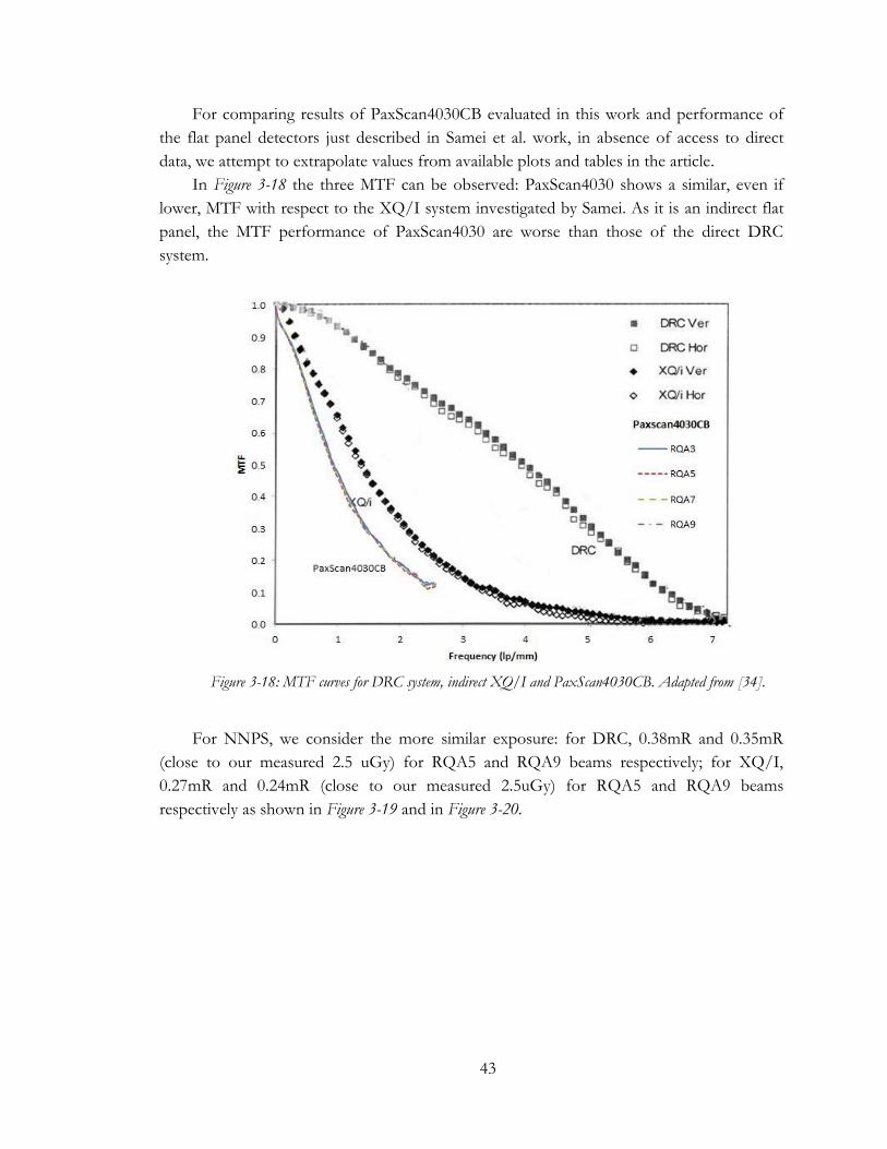
43

For comparing results of PaxScan4030CB evaluated in this work and performance of

the flat panel detectors just described in Samei et al. work, in absence of access to direct

data, we attempt to extrapolate values from available plots and tables in the article.

In Figure 3-18 the three MTF can be observed: PaxScan4030 shows a similar, even if

lower, MTF with respect to the XQ/I system investigated by Samei. As it is an indirect flat

panel, the MTF performance of PaxScan4030 are worse than those of the direct DRC

system.

Figure 3-18: MTF curves for DRC system, indirect XQ/I and PaxScan4030CB. Adapted from [34].

For NNPS, we consider the more similar exposure: for DRC, 0.38mR and 0.35mR

(close to our measured 2.5 uGy) for RQA5 and RQA9 beams respectively; for XQ/I,

0.27mR and 0.24mR (close to our measured 2.5uGy) for RQA5 and RQA9 beams

respectively as shown in Figure 3-19 and in Figure 3-20.

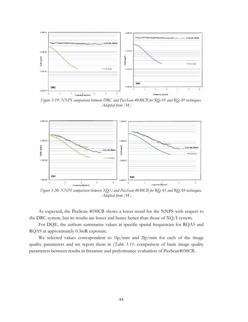
44

Figure 3-19: NNPS comparison between DRC and PaxScan 4030CB for RQA5 and RQA9 techniques.

Adapted from [34].

Figure 3-20: NNPS comparison between XQ/i and PaxScan 4030CB for RQA5 and RQA9 techniques.

Adapted from [34].

As expected, the PaxScan 4030CB shows a lower trend for the NNPS with respect to

the DRC system, but its results are lower and hence better than those of XQ/I system.

For DQE, the authors summarize values at specific spatial frequencies for RQA5 and

RQA9 at approximately 0.3mR exposure.

We selected values correspondent to 1lp/mm and 2lp/mm for each of the image

quality parameters and we report them in (Table 3-11: comparison of basic image quality

parameters between results in literature and performance evaluation of PaxScan4030CB..

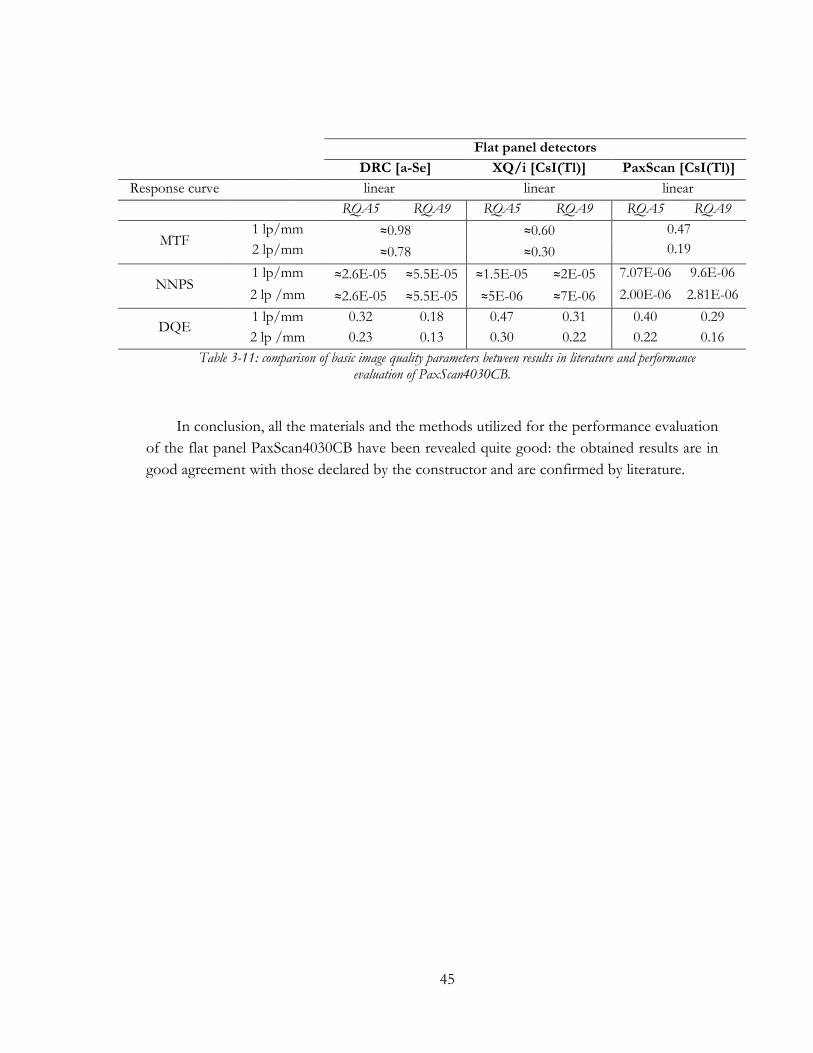
45

Flat panel detectors

DRC [a-Se] XQ/i [CsI(Tl)] PaxScan [CsI(Tl)]

Response curve linear linear linear

RQA5 RQA9 RQA5 RQA9 RQA5 RQA9

MTF 1 lp/mm ≈0.98

≈0.78

≈0.60

≈0.30

0.47

0.19 2 lp/mm

NNPS 1 lp/mm ≈2.6E-05 ≈5.5E-05 ≈1.5E-05 ≈2E-05 7.07E-06 9.6E-06

2 lp /mm ≈2.6E-05 ≈5.5E-05 ≈5E-06 ≈7E-06 2.00E-06 2.81E-06

DQE 1 lp/mm 0.32 0.18 0.47 0.31 0.40 0.29

2 lp /mm 0.23 0.13 0.30 0.22 0.22 0.16

Table 3-11: comparison of basic image quality parameters between results in literature and performance evaluation of PaxScan4030CB.

In conclusion, all the materials and the methods utilized for the performance evaluation

of the flat panel PaxScan4030CB have been revealed quite good: the obtained results are in

good agreement with those declared by the constructor and are confirmed by literature.

46

47

Chapter 4 Conclusions

The aim of this thesis was the quality assessment of the fluoroscopic chain available in

the laboratory of the Centre of Medical Physics at the Policlinico S.Orsola.

The X-ray source RTM70H IAE has been studied in its output efficiency for the RQA

series and, for a detailed knowledge of the shape of the recreated spectra, RQA beams have

been simulated with SpekCalc algorithm.

The physical characterization of the PaxScan 4030CB Varian flat panel has been

performed: the detector has been tested in its linear response and the basic parameters for

image quality assessment, such as MTF, NNPS and DQE, have been evaluated.

Using the RQA techniques, the most widespread material and methods have been used

to acquire the images necessary to the evaluation of MTF, NNPS and DQE. Hence, the

calculation of these objective parameters have been done with the aid of the COQ plug-in

for ImageJ suite.

The PaxScan4030CB shows a good MTF, a very low noise evaluated with NNPS and a

high DQE. Qualitative information on the flat panel performance have been extracted

through a low-contrast sensitivity phantom.

The results obtained in this work are consistent with respect to the performance of

other indirect flat panel detectors studied in literature.

This work is the starting point for the complete characterization of the PaxScan

4030CB flat panel. Future developments will be a psycophysical characterization and then an

analysis of dynamic phantoms with different contrast media, in particular carbon dioxide in

DSA.

The goal will be the establishment of the best working conditions for PaxScan 4030CB

and RTM70H X-ray source to get the best images with the lowest patient dose for different

clinical exams.

48

49

Bibliography

[1] M. McDonald, «A Method to Measure the Detective Quantum Efficiency of

Radiographic Systems in a Clinical Setting,» Graduate Program in Biomedical

Engineering, Ontario, 2012.

[2] J. Beutel, H. L. Kundel e R. L. Van Metter, Handbook of Medical Imaging, Vol.1

Physics and Psycophysics, Washington: Spie Press, 2000.

[3] D. Dance, S. Christofides, A. Maidment, I. McLean e K. Ng, Diagnostic radiology

physics : a handbook for teachers and students, Vienna: IAEAL, 2014.

[4] J. T. Bushberg, J. A. Seibert, E. M. Leidholdt e J. M. Boone, The Essential Physics of

Medical Imaging, Philadelphia: Lippincott Williams & Wilkins, 2002.

[5] E. L. Nickoloff, «AAPM/RSNA Physics Tutorial for Residents: Physics of Flat-Panel

Fluoroscopy Systems. Survey of Modern Fluoroscopy Imaging: Flat-Panel Detectors

versus Image Intensifiers,» RadioGraphics , n. 31, p. 591–602, 2011.

[6] M. Spahn, «Flat detectors and their clinical applications,» Eur Radiol, n. 15, p. 1934–

1947, 2005.

[7] I. Siemens Medical Solutions USA, «White Paper | Dynamic Flat-Panel Detectors in

Fluoroscopy - Technology and Clinical Advantages,» Malvern, PA, 2013.

[8] V. Tsapaki, S. Kottou e N. Kollaros, «Comparison of a conventional and a flat-panel

digital system in interventional cardiology procedures.,» The British Journal of Radiology, n.

77, p. 562–567, 2004.

[9] B. Wiesinger, A. Stütz, J. Schmehl, C. D. Claussen e J. Wiskirchen, «Comparison of

Digital Flat-Panel Detector and Conventional Angiography Machines: Evaluation of

Stent Detection Rates, Visibility Scores, and Dose-Area Products,» American Journal of

Roentgenology, n. 198, p. 946–954, 2012.

[10] A. Davies, A. Cowen, S. Kengyelics, J. Moore e M. Sivananthan, «Do flat detector

cardiac X-ray systems convey advantages over image-intensifier-based systems? Study

50

comparing X-ray dose and image quality,» Journal of European Radiology, n. 17, p. 1787–

1794, 2007.

[11] S. Rivetti, «Performance evaluation of detectors for digital radiography,» in Dottorato di

ricerca in Fisica (FIS/07: Fisica Applicata), Alma Mater Studiorum, Bologna, Ciclo XXIII,

Marzo 2011.

[12] A. Rose, «The sensitivity performance of the human eye on the absolute scale,» Journal of

the Optical Society of America, vol. 38, p. 196–208, 1948.

[13] E. Samei, «Performance of Digital Radiographic Detectors: Quantification and

Assessment Methods,» Advances in Digital Radiography: RSNA Categorical Course in

Diagnostic Radiology Physics, p. 37–47, 2003.

[14] H. Fujita, D. Tsai, T. Itoh, K. Doi, J. Morishita, K. Ueda e A. Ohtsuka, «A simple

method for determining the Modulation Transfer Function in Digital Radiography,»

IEEE Transactions on Medical Imaging, vol. 11, n. 1, pp. 34-39, 1992.

[15] E. Samei, M. J. Flynn e D. A. Reimann, «A method for measuring the presampled MTF

of digital radiographic systems using an edge test device,» Medical Physics , vol. 1, n. 25,

pp. 102-113, January 1998.

[16] J. T. Dobbins III, E. Samei, N. T. Ranger e Y. Chen, «Intercomparison of methods for

image quality characterization. II .Noise power spectrum,» Medical Physics, vol. 33, n. 5,

pp. 1466-1467, 2006.

[17] J. M. Boone e J. A. Seibert, «An accurate method for computer-generating tungsten

anode x-ray spectra from 30 to 140 kV,» Medical Physics , vol. 24 , n. 11, pp. 1661-1670,

1997.

[18] I.A.E., «Documentazione Tubo a Raggi X - RTM70H,» I.A.E. Spa, MI, 2013.

[19] I. Varian Medical Systems, «PaxScan 3030CB/4030CB Systems and Service Guide

(P/N 20099),» Salt Lake City, February 2010.

[20] W. Zhao, G. Ristic e J. A. Rowlands, «X-ray imaging performance of structured cesium

iodide scintillators,» Medical Physics , vol. 9, n. 31 , pp. 2594-2605, 2004.

[21] M. S. Varian, «X-ray Products -- PaxScan4030CB Digital Image Receptor,» Varian, Salt

Lake City, 2012.

[22] A. Cowen, A. Daviesa e M. Sivananthan, «The design and imaging characteristics of

dynamic, solid-state, flat-panel x-ray image detectors for digital fluoroscopy and

fluorography,» Clinical Radiology , n. 63, pp. 1073-1085, 2008 .

[23] B. Donini, S. Rivetti, N. Lanconelli e M. Bertolini, «Free software for performing

physical analysis of systems for digital radiography and mammography,» Medical Physics,

vol. 41, n. 5, pp. 051903-1/10, 2014.

[24] B. Donini, S. Rivetti, N. Lanconelli e M. Bertolini, «COQ: an ImageJ plugin for the

physical characterization and quality checks of digital detectors.,» Bologna, 2014.

51

[25] International Electrotechnical Commission, «Medical electrical equipment -

Characteristics of digital X-ray imaging devices Part 1: Determination of the detective

quantum efficiency - Detectors used in dynamic imaging,» IEC- 62220–1, Geneva,

Switzerland, 2010.

[26] E. Samei, M. J. Flynn e D. A. Reimann, «A method for measuring the presampled MTF

of digital radiographic systems using an edge test device,» Medical Physics, vol. 25, n. 102,

1998.

[27] J. T. I. Dobbins, «Image quality metrics for digital systems,» in Handbook of Medical

Imaging, Vol. 1, WA, SPIE, 2000, p. 161–222.

[28] A. RTI Electronics, «Barracuda User's Manual - Version 1.4A,» Molndal, 2004.

[29] C. E. 61267, «Medical diagnostic X-ray equipment - Radiation conditions for use in the

determination of characteristics,» CEI, Milano, 2006-10.

[30] G. Poludniowski, G. Landry, F. DeBlois, P. Evans e F. Verhaegen, «SpekCalc: a

program to calculate photon spectra from tungsten anode x-ray tubes».

[31] G. Borasi, A. Nitrosi, P. Ferrari e D. Tassoni, «On site evaluation of three flat panel

detectors for digital radiography,» Medical Physics, vol. 30, n. 7, 2003.

[32] S. Rivetti, N. Lanconelli, M. Bertolini, A. Nitrosi e A. Burani, «Characterization of a

clinical unit for digital radiography based on irradiation side sampling technology,»

Medical Physics , vol. 10, n. 40 , 2013.

[33] B. Zhao, X. Qin, Z. Feng, C. Wei, Y. Chen, B. Wang e L. Wei, «Performance evaluation

of CsI screens for X-ray imaging,» Chinese Physics C, vol. 38, n. 11, 2014.

[34] E. Samei e M. Flynn, «An experimental comparison of detector performance for direct

and indirect digital radiography systems,» Medical Physics, vol. 4, n. 30, pp. 608-615, 2003.

[35] IAE, «Tecnologia dei tubi radiogeni,» Industria Applicazioni Elettroniche SpA, Milano,

2010.

[36] J. T. I. Dobbins, D. L. Ergun, L. Rutz, D. A. Hinshaw, H. Blume e D. Clark, « DQE(f)

of four generations of computed radiography acquisition devices,» Medical Physics, n. 22,

p. 1581–1593, 1995.

[37] T. Gomi, K. Koshida, T. Miyati, J. Miyagawa e H. Hirano, «An Experimental

Comparison of Flat-Panel Detector Performance for Direct and Indirect Systems

(Initial Experiences and Physical Evaluation),» Journal of Digital Imaging, vol. 19, n. 4, pp.

362-370, 2006.