Performance Analysis with the IBM Full-System Simulator - iLab!

Performance Analysis with the IBM Full-System SimulatorModeling the Performance of the Cell Broadband Engine Processor

Version 3.0© International Business Machines Corporation

Performance Analysis with the IBM Full-System Simulator

© International Business Machines Corporation (2007). All Rights Reserved.

Printed in the United States of America September 2007.

No part of this publication may be reproduced, transmitted, transcribed, stored in a retrieval system, or translated into any

computer language, in any form or by any means, electronic, mechanical, magnetic, optical, chemical, manual, or otherwise,

without prior written permission of IBM Corporation. No other rights under copyright are granted without prior written

permission of IBM Corporation.

While the information contained herein is believed to be accurate, such information is preliminary, and should not be relied

upon for accuracy or completeness, and no representations or warranties of accuracy or completeness are made. All

information contained in this document is subject to change without notice. This document contains information on products

in the design, sampling and/or initial production phases of development. This information is subject to change without notice,

and is provided without warranty of any kind. The information contained in this document does not affect or change IBM

product specifications or warranties. Nothing in this document shall operate as an express or implied license or indemnity

under the intellectual property rights of IBM or third parties. All information contained in this document was obtained in specific

environments, and is presented as an illustration. The results obtained in other operating environments may vary. The

document is not intended for production.

THE INFORMATION CONTAINED IN THIS DOCUMENT IS PROVIDED ON AN “AS IS” BASIS. In no event will IBM be liable for

damages arising directly or indirectly from any use of the information contained in this document.

U.S. Government Users Restricted Rights—Use, duplication or disclosure restricted by GSA ADP Schedule Contract with IBM

Corporation.

IBM is a registered trademark of International Business Machines Corporation in the United States, other countries, or both. The

IBM logo, PowerPC, PowerPC logo, and PowerPC architecture are trademarks of International Business Machines Corporation

in the United States, or other countries, or both.

Linux is a registered trademark of Linus Torvalds. Linux is written and distributed under the GNU General Public License in the

United States and other countries.

Other company, product, and service names may be trademarks or service marks of others.

The IBM home page can be found at www.ibm.com.

SysSimPerfAnalysisGuide, Version 3.0

Contents

Preface . . . . . . . . . . . . . . . . . . . . . . . . . . . . . . . . . . . . . . . . . . . . . . . . . . . . . . . . . . . . . . . . . . . . . . . . . . . . . . v

1 Performance Simulation and Analysis with the IBM Full-System Simulator . . . . . . . . . . . . . . . . . . 1

An Overview of the IBM Full-System Simulator . . . . . . . . . . . . . . . . . . . . . . . . . . . . . . . . . . . . . . . . . . . . . . . . . . . . 2

Modeling the CBE Architecture in the IBM Full-System Simulator . . . . . . . . . . . . . . . . . . . . . . . . . . . . . . . . . . . . 3

Running Applications in the IBM Full-System Simulator . . . . . . . . . . . . . . . . . . . . . . . . . . . . . . . . . . . . . . . . . . . . . 4

2 Performance Modeling with the IBM Full-System Simulator . . . . . . . . . . . . . . . . . . . . . . . . . . . . . . . 5

Performance Modeling with SystemSim . . . . . . . . . . . . . . . . . . . . . . . . . . . . . . . . . . . . . . . . . . . . . . . . . . . . . . . . . . 6

Synergistic Processing Elements (SPEs) . . . . . . . . . . . . . . . . . . . . . . . . . . . . . . . . . . . . . . . . . . . . . . . . . . . . . . . . . 6

L1 and L2 Caches. . . . . . . . . . . . . . . . . . . . . . . . . . . . . . . . . . . . . . . . . . . . . . . . . . . . . . . . . . . . . . . . . . . . . . . . . . . . 6

Element Interconnect Bus . . . . . . . . . . . . . . . . . . . . . . . . . . . . . . . . . . . . . . . . . . . . . . . . . . . . . . . . . . . . . . . . . . . . 6

Memory Interface Controller and System Memory . . . . . . . . . . . . . . . . . . . . . . . . . . . . . . . . . . . . . . . . . . . . . . 6

Enabling the Performance Models in a Simulation . . . . . . . . . . . . . . . . . . . . . . . . . . . . . . . . . . . . . . . . . . . . . . . . . 7

From the Graphical User Interface. . . . . . . . . . . . . . . . . . . . . . . . . . . . . . . . . . . . . . . . . . . . . . . . . . . . . . . . . . . . . 7

From the Command Line. . . . . . . . . . . . . . . . . . . . . . . . . . . . . . . . . . . . . . . . . . . . . . . . . . . . . . . . . . . . . . . . . . . . . 8

Gathering Performance Metrics. . . . . . . . . . . . . . . . . . . . . . . . . . . . . . . . . . . . . . . . . . . . . . . . . . . . . . . . . . . . . . . . . . 8

3 Performance Analysis with Profile Checkpoints and Triggers. . . . . . . . . . . . . . . . . . . . . . . . . . . . .11

Viewing SPU Performance Statistics . . . . . . . . . . . . . . . . . . . . . . . . . . . . . . . . . . . . . . . . . . . . . . . . . . . . . . . . . . . . .12

Capturing Performance Data in a TCL Array . . . . . . . . . . . . . . . . . . . . . . . . . . . . . . . . . . . . . . . . . . . . . . . . . . . . .15

Instrumenting SPU Applications with Performance Profile Checkpoints . . . . . . . . . . . . . . . . . . . . . . . . . . . . .15

Enhancing Data Collection with Triggers . . . . . . . . . . . . . . . . . . . . . . . . . . . . . . . . . . . . . . . . . . . . . . . . . . . . . . . .17

Tutorial: Collecting Performance Data with Checkpoints and Triggers . . . . . . . . . . . . . . . . . . . . . . . . . . . . . .19

4 Performance Data Collection and Analysis with Emitters . . . . . . . . . . . . . . . . . . . . . . . . . . . . . . . .23

Emitter Architecture Overview. . . . . . . . . . . . . . . . . . . . . . . . . . . . . . . . . . . . . . . . . . . . . . . . . . . . . . . . . . . . . . . . . .24

Underlying Emitter Record Data Structure . . . . . . . . . . . . . . . . . . . . . . . . . . . . . . . . . . . . . . . . . . . . . . . . . . . . . . .25

Configuring Emitter Event Production . . . . . . . . . . . . . . . . . . . . . . . . . . . . . . . . . . . . . . . . . . . . . . . . . . . . . . . . . . .25

Specifying Events to Produce Emitter Data . . . . . . . . . . . . . . . . . . . . . . . . . . . . . . . . . . . . . . . . . . . . . . . . . . . .26

Configuring the Number of Emitter Readers. . . . . . . . . . . . . . . . . . . . . . . . . . . . . . . . . . . . . . . . . . . . . . . . . . .26

Starting Emitter Readers . . . . . . . . . . . . . . . . . . . . . . . . . . . . . . . . . . . . . . . . . . . . . . . . . . . . . . . . . . . . . . . . . . . . .26

Tutorial: Configuring Emitter Event Production . . . . . . . . . . . . . . . . . . . . . . . . . . . . . . . . . . . . . . . . . . . . . . . . . . .26

Developing Emitter Readers to Process Event Data . . . . . . . . . . . . . . . . . . . . . . . . . . . . . . . . . . . . . . . . . . . . . . .27

Tutorial: Developing a Basic Emitter Reader . . . . . . . . . . . . . . . . . . . . . . . . . . . . . . . . . . . . . . . . . . . . . . . . . . . . . .28

A SPU Performance Statistics . . . . . . . . . . . . . . . . . . . . . . . . . . . . . . . . . . . . . . . . . . . . . . . . . . . . . . . . . . .33

iii© International Business Machines Corporation. All rights reserved.

Preface

Analyzing the performance of distributed, real-time, and embedded systems is a challenging task due to the

complexity and low-level nature of such systems. The IBM Full System Simulator project (SystemSim) strives to build

tools and frameworks that enable software designers to evaluate and visualize the performance of a modeled

processor system. With this insight, designers are able to pinpoint bottlenecks in a system and optimize its

performance.

The Performance Analysis Using SystemSim guide describes the performance analysis methodology and

implementation techniques developed to collect and analyze performance metrics for software systems executing on

the IBM Full-System simulator.

Intended AudienceThis document is intended for designers and programmers who are evaluating the performance of applications and

systems software for systems based on the Cell Broadband Engine Architecture (CBEA). Potential users include:

System and software designers

Hardware and software tool developers

Application and product engineers

Validation engineers

Using This Version of the GuideThis version of the Performance Analysis with the IBM Full-System Simulator applies to version 2.1 of the IBM Full-

System Simulator for the Cell Broadband Engine Processor, available from IBM’s alphaWorks Emerging Technologies

website located at http://www.alphaworks.ibm.com/tech/cellsystemsim.

The guide is organized into topics that cover concepts and procedures for capturing a variety of performance metrics

for CBEA applications using performance analysis techniques. This book includes the following chapters and

appendices:

Chapter 1, Performance Simulation and Analysis with the IBM Full-System Simulator, describes the IBM Full

System Simulator developed by the IBM Austin Research Lab (ARL), and introduces the Cell Broadband Engine

Architecture (CBEA) modeled by the IBM Full-System Simulator.

Chapter 2, “Performance Modeling with the IBM Full-System Simulator,” provides information about

performance modeling support in the IBM Full-System Simulator, including descriptions of components for

which performance simulation is currently available. It also describes how to enable performance simulation

from the simulator command line and graphical user interface.

v© International Business Machines Corporation. All rights reserved.

Chapter 3, Performance Analysis with Profile Checkpoints and Triggers, describes performance profile

checkpoint and trigger functionality, and illustrates how these mechanisms are used to generate application-

specified performance data in a simulation.

Chapter 4, Performance Data Collection and Analysis with Emitters, describes the IBM Full-System Simulation

emitter architecture. This section contains a tutorial that describes how to configure the simulator to emit event

data, and how to develop emitter readers to analyze the emitted event data. This chapter also describes how to

enhance emitter reader functionality with annotations.

Appendix A, SPU Performance Statistics, lists the checkpoint types that were gathered during performance

evaluation.

Typographical ConventionsThe following typographical components are used for defining special terms and command syntax:

Table 1. Typographical Conventions

Convention Description

Bold typeface Represents literal information, such as:

Information and controls displayed on screen, including menu options, application pages, windows, dialogs, and field names.

Commands, file names, and directories.

In-line programming elements, such as function names and XML elements when referenced in the main text.

Italics typeface Italics font is used to emphasize new concepts and terms, and to stress important ideas. Additionally, book and chapter titles are displayed in italics.

Sans serif typeface Represents example code output, such as XML output or C/C++ code examples.

Italic sans serif words or characters in code and commands represent values for variables that you must supply, such as arguments to commands or path names for your particular system. For example: cd /users/your_name

... (Horizontal or Vertical ellipsis)

.

.

.

In format and syntax descriptions, an ellipsis indicates that some material has been omitted to simplify a discussion.

{ } (Braces) Encloses a list from which you must choose an item or information in syntax descriptions.

[ ] (Brackets) Encloses optional items in format and syntax descriptions. For example, in the statement SELECT [DISTINCT], DISTINCT is an optional keyword.

| (Vertical rule) Separates items in a list of choices enclosed in { } (braces) in format and syntax descriptions.

UPPERCASE Indicates keys or key combinations that you can use. For example, press CTRL + ALT + DEL.

Hyperlink Web-based URIs are displayed in blue text to denote a virtual link to an external document. For example: http://www.ibm.com

The note block denotes information that emphasizes a concept or provides peripheral information.NOTE This is note text.

vi Preface © IBM Corporation. All rights reserved.

Related Guides and Recommended ReferenceThe IBM Full-System Simulator User’s Guide describes the basic structure and operation of the IBM Full-System

Simulator and its graphic user interface (GUI) and command line user interface. The IBM Full-System Simulator User’s

Guide is commonly distributed with alphaWorks releases in the docs directory as SystemSim.Users.Guide.pdf.

The IBM Austin Research Lab also recommends the following documentation sources that may provide helpful

guidelines and background information about technologies used in the simulation environment:

Practical Programming in Tcl and Tk by Brent B. Welch. Prentice Hall, Inc.

Contacting the IBM Full-System Simulator Development TeamThe IBM Full-System Simulator development team at ARL is very interested in hearing from you about your experience

with the IBM Full-System Simulator and its supporting information set. Should you have questions or encounter any

issues with the IBM Full-System Simulator, visit the project forum at

http://www.alphaworks.ibm.com/tech/cellsystemsim/forum.

viiPreface

CHAPTER 1

Performance Simulation and Analysis withthe IBM Full-System Simulator

This chapter provides an overview of the IBM Full System Simulator, SystemSim, developedby the IBM Austin Research Lab (ARL), and introduces the Cell Broadband EngineArchitecture (CBEA) that is modeled by SystemSim. It also describes configuration parametersfor setting up and running the simulation environment in standalone and Linux mode.Topics in this chapter include:

An Overview of the IBM Full-System Simulator

Modeling the CBE Architecture in the IBM Full-System Simulator

Running Applications in the IBM Full-System Simulator

1© International Business Machines Corporation. All rights reserved.

An Overview of the IBM Full-System SimulatorThe IBM Full-System Simulator (SystemSim) provides fast but accurate simulation of complete systems with processors

that are based on the IBM PowerPC Architecture. SystemSim, originally known by the internal IBM name “Mambo,”

contains numerous features to support software design and analysis, including parameterized models for

architectural features and dynamically selectable model fidelity that enable users to trade simulation accuracy for

execution speed. SystemSim has been used extensively inside IBM to support the development of operating systems,

compilers, and key software components for new systems well in advance of hardware availability.

The IBM Full-System Simulator is a sophisticated simulation environment that supports both functional and

performance simulation of multiple PowerPC cores and a variety of system components. The simulator’s processor

support includes interrupts, debugging controls, caches, busses, and a large number of architectural features. In

addition, The simulator models memory-mapped I/O devices, consoles, disks, and networks that allow operating

systems to run in simulation, and boot and run programs.

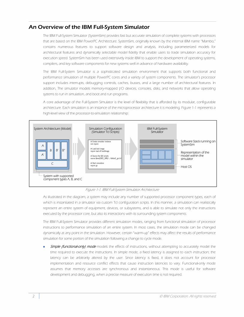
A core advantage of the Full-System Simulator is the level of flexibility that is afforded by its modular, configurable

architecture. Each simulation is an instance of the microprocessor architecture it is modeling. Figure 1-1 represents a

high-level view of the processor-to-simulation relationship:

Figure 1-1. IBM Full-System Simulator Architecture

As illustrated in the diagram, a system may include any number of supported processor component types, each of

which is instantiated in a simulator via custom Tcl configuration scripts. In this manner, a simulation can realistically

represent an entire system of equipment, devices, or subsystems, and is able to simulate not only the instructions

executed by the processor core, but also its interactions with its surrounding system components.

The IBM Full-System Simulator provides different simulation modes, ranging from functional simulation of processor

instructions to performance simulation of an entire system. In most cases, the simulation mode can be changed

dynamically at any point in the simulation. However, certain “warm-up” effects may affect the results of performance

simulation for some portion of the simulation following a change to cycle mode.

Simple (functional-only) mode models the effects of instructions, without attempting to accurately model the

time required to execute the instructions. In simple mode, a fixed latency is assigned to each instruction; the

latency can be arbitrarily altered by the user. Since latency is fixed, it does not account for processor

implementation and resource conflict effects that cause instruction latencies to vary. Functional-only mode

assumes that memory accesses are synchronous and instantaneous. This mode is useful for software

development and debugging, when a precise measure of execution time is not required.

System Architecture (Model)

A

A'B B' B''

C

# Create simulator instancesim mysim

# Load boot imagemysim load elf bootImage

# Source the GUI scriptssource $env(EXEC_DIR)/../default_gui.tcl

# Start simulationmysim go

System with supported component types A, B, and C

Simulation Configuration (Simulator Tcl Scripts)

IBM Full-System Simulator

Representation of the model within the simulator

Host OS

Software Stack running on SystemSim

2 © IBM Corporation. All rights reserved.

Fast mode is similar to functional-only mode in that it fully models the effects of instructions while making no

attempt to accurately model execution time. In addition, fast mode bypasses many of the standard analysis

features provided in functional-only mode, such as statistics collection, triggers, and emitter record generation.

Fast mode simulation is intended to be used to quickly advance the simulation through uninteresting portions of

program execution to a point where detailed analysis is to be performed.

Cycle (performance) mode. models not only functional accuracy but also timing. It considers internal execution

and timing policies as well as the mechanisms of system components, such as arbiters, queues, and pipelines.

Operations may take several cycles to complete, accounting for both processing time and resource constraints.

These simulation modes are used to support concurrent development and performance evaluation of a number of

software and hardware systems. The primary objective of this focus is to enable internal teams and IBM partners to:

Use the simulator to gather and compare performance data with a greater level of fidelity.

Characterize the workload on the system.

Forecast performance at future loads and fine-tune performance benchmarks for future validation.

The IBM Full-System Simulator also includes trace collection and debugging interfaces to allow detailed analysis of the

simulated hardware and software.

Modeling the CBE Architecture in the IBM Full-System SimulatorIn 2001, Sony, Toshiba, and IBM (STI) combined research and development efforts to create an advanced Cell

Broadband Engine Processor (CBEP) for a new wave of devices in the emerging broadband era. Shortly after project

inception, STI engaged the IBM Austin Research Laboratory (ARL) to model the Cell Broadband Engine processor to

support software simulation and performance testing using the IBM Full-System Simulator.

Initially, the IBM Full-System Simulator Cell model supported functional simulation of the PPE and SPU processors. The

ARL development team incorporated a standalone simulator for SPU programs (called apusim) into the simulator to

provide SPU simulation functionality. The apusim simulator was developed by the STI Design Center and supported

both functional and performance simulation of standalone SPU programs. In the IBM Full-System Simulator, SPU

program execution can be performed in either instruction mode, which performs functional simulation only, or

pipeline mode, which performs functional and performance simulation. In pipeline mode, the behavior of the SPU

execution pipeline is modeled in detail and statistics on pipeline operation are collected. However, SPU instructions

that interact with other parts of the system, such as the MFC channels or DMA operations, are only modeled at the

functional level.

3Performance Simulation and Analysis with the IBM Full-System Simulator

Figure 1-2 illustrates the high-level view of the CBE architecture modeled by the IBM Full-System Simulator.

Figure 1-2. High-Level Block Diagram of the Simulated CBEA

Running Applications in the IBM Full-System SimulatorA key attribute of the IBM Full-System Simulator is its ability to boot and run a complete PowerPC system. By booting

an operating system, such as Linux, the simulator can execute many typical application programs that utilize standard

operating system functionality. When Linux is booted in the simulator, the Linux operating system (running in the

simulated environment) loads the application and is responsible for all operating system calls.

Alternatively, applications can be run in standalone mode, in which all operating system functions are supplied by the

simulator and normal operating system effects do not occur, such as paging and scheduling. In standalone mode,

the simulator simply loads the application into simulated memory and begins the simulation at the application's entry

point. The simulator can also execute SPU programs in standalone mode on a given SPU. This mode provides

information that is more directly a result of the intrinsic program design and implementation. This is useful for

application’s performance measurement and analysis.

The IBM Full-System Simulator User’s Guide describes the commonly used commands to create full-system or

standalone simulation environments.

SPE Core #0

Cell Broadband Engine

SPE Core #1 SPE Core #7

. . .

PPE

SPU PPU UnitPPU

L1

CIU

NCU

MMU

RMT

Storage Subsystem

L2 RMT

BIUBIU

SPX

LS

DMA

ATO MMURMT

MFC

SPU

BIU

SPX

LS

DMA

ATO MMURMT

MFC

SPU

BIU

SPX

LS

DMA

ATO MMURMT

MFC

Element Interconnect (EIB)

BICI/O CtrlI/O TransI/O CtrlBIC MIC

ATO Atomic unit LS Local storage

EIB Element Interconnect bus MFC Memory flow controller

BEI Broadband engine interface unit MIC Memory interface controller

BIC Bus interface controller MMU Memory manamgement unit

BIU (or SBI) Bus interface unit NCU Non-coherent unit

CIU Coherence interface unit PPC PowerPC processing core

DMA Direct Memory Access PPU PowerPC Processing unit

IOC I/O interface controller RMT Replacement management table

L1 Level 1 cache SPC Synergistic processing core

L2 Level 2 cache SPU Synergistic processing core

4 Running Applications in the IBM Full-System Simulator © IBM Corporation. All rights reserved.

CHAPTER 2

Performance Modeling with theIBM Full-System Simulator

This chapter provides information about performance modeling support in the IBM Full-System Simulator, including descriptions of components for which performance simulation iscurrently available. It also describes how to enable performance simulation from thesimulator command line and graphical user interface. Topics in this chapter include:

Performance Modeling with SystemSim

Enabling the Performance Models in a Simulation

Gathering Performance Metrics


Performance Modeling with SystemSimSupport for performance simulation has been evolving since the IBM Full-System Simulator for the Cell Broadband

Engine platform was originally released on alphaWorks. The first version of the simulator provided a cycle-accurate

model of the SPU interactions, which enabled developers to gather detailed performance data about the execution

of SPU programs, such as pipeline stalls, operand dependencies, and so forth. Subsequent versions of the simulator

have provided performance simulation of memory subsystem functions (in version 2.0) and the PPU execution (in

version 2.1). As a result, the simulator now supports performance simulation for nearly all aspects of the Cell

Broadband Engine processor operation.

It is important to note that the simulator provides significant timing information about processor components, and

has proven very useful in exploring the functionality and performance of Cell/B.E. based processor systems. However,

running on hardware provides the most definitive performance results, and should be used when precise

performance information is needed.

Synergistic Processing Elements (SPEs)

Systemsim accurately models the microarchitectural flow of instructions through the SPU pipelines, including

instruction prefetch logic, branch hint and mispredict behaviors, issue stall conditions, execution latencies, and

resource contention. The SPU pipeline model includes extensive instrumentation to provide performance metrics and

cycle-level tracing. The MFC performance model includes bus interface unit queues and policies, DMA engine

queues and state machines, address translation engine behaviors, and the atomic cache. SystemSim’s MFC model

unrolls DMA single and list commands into their individual transaction components. These are processed by the

various state machine engines, collect in queues, and flow across interconnects in order to capture the latency and

bandwidth effects of arbitration policies, queue management, and resource contention.

L1 and L2 Caches

Since cache utilization can play a significant role in system and application performance, the simulator provides the

ability to accurately model and measure the performance of a cache subsystem. The simulator cache models for the

L1 and L2 caches provide performance metrics that are useful in analyzing PPE performance. The L1 and L2 caches

are accurately modeled in terms of size, associativity, replacement policies, and latency. Currently the cache models

do not support the Replacement Management Table (RMT) features of the CBE architecture.

Element Interconnect Bus

The Element Interconnect Bus (EIB) model handles the complex rules for managing data coherence as specified in

the Broadband Interface Protocol (BIF), including command formats, transaction types, and the snooper cache

coherence protocol for the CELL processor system. Rather than using a simplistic “method call or function call-back”

approach, the simulator models the flow of bus transactions. including out-of-order transaction support, split

transaction designs, arbitration policies, fragmenting (scatter/gather), and flow control. This design enables

transactions to be tracked accurately through the data analysis framework.

Memory Interface Controller and System Memory

The Memory Interface Controller (MIC) model connects the EIB to the off-chip system memory and manages the flow

of data onto and off of the Cell Broadband Engine processor from system memory. The MIC model also supports

scheduling policies between the read queue and write queue in order to minimize latency and implements a snoop-

based cache coherence.


The simulator currently does not provide a model for RAMBUS architecture memory; instead it contains a

performance model for DDR2 SDRAM memory that is configured to approximate the performance of the RAMBUS

XDR memory used by the Cell processor.

Enabling the Performance Models in a SimulationThe performance models described above can be enabled from the GUI using the performance models dialog or

with simulator commands. The performance models can be enabled at any time after the simulated machine has

been defined, but typically are not enabled until after the operating system has been booted. To enable the

performance models in a simulation, complete the following steps:

From the Graphical User Interface

To enable the performance models from the graphical user interface:

1. Click the Mode button on the main GUI window.

Figure 2-1. SystemSim Cell Graphical User Interface

2. SystemSim displays the simmodes window containing a message indicating the current simulation mode and

three buttons which will change the simulation mode to fast, simple, or cycle mode. Figure 2-2 shows an

example of this dialog window. This dialog provides a convenient way to set the simulation mode for

components of the system in a consistent manner. The simulation mode can also be selected with the “mysim

mode” command and displayed with the “mysim display mode” command.

Figure 2-2. Simulation Mode Window

3. The simulator also provides the SPU Modes dialog to set each SPU's simulation mode to instruction mode,

pipeline (cycle accurate) mode or fast mode. The SPU Modes dialog, shown in Figure 2-3, is accessed from the

7Performance Modeling with the IBM Full-System Simulator

SPU Modes button on the main GUI window. If the simulator is launched in SMP mode, this dialog will show all

the SPUs in both BEs; otherwise only the SPUs for BE 0 are displayed.

Figure 2-3. SystemSim SPU Modes

a. For each individual SPU, click the level of timing mode to simulate: Pipe, Instruction, or Fast. The SPU mode

for an individual SPU can also be selected using the Model toggle menu sub-item under each SPE in the

tree menu at the left of the main control panel.

b. To enable the same timing mode for all SPUs in the BE, click the corresponding button.

c. Click Refresh to synchronize the window with any changes to the modeling mode that may have been updated by the command line interface or the tree view.

4. Click Go in the main GUI window to start the simulation with performance models enabled.

From the Command Line

To enable all performance models from the command line, type the following command:

turn_perf_models_on

Gathering Performance MetricsThe simulator provides an extensive variety of data collection and analysis capabilities, including the following

mechanisms:

Performance Profiling Checkpoints. Performance profile checkpoints provide the most basic level of code

instrumentation for gaining insight into SPU performance. The simulator provides a set of checkpoint instructions

that can be added to a region of code to control the collection and display of SPU performance data. These

instructions offer a very lightweight, minimally intrusive mechanism for the user to obtain performance

information for SPU program execution. See Chapter 3, “Performance Analysis with Profile Checkpoints and

Triggers,” for information and instructions for adding performance profile checkpoints to application code.

Triggers. Triggers can be used to invoke user-supplied TCL procedures to collect and aggregate performance

data when specific types of simulation events occur. This general-purpose mechanism can be used to

implement a variety of breakpoints, accumulate metrics, produce messages, or perform any number of tasks that

are supported in a TCL procedure. The simulator provides trigger events for the program counter, memory

accesses, cycle counts, console output strings, and a number of simulation events. See Chapter 3, “Performance

Analysis with Profile Checkpoints and Triggers,” for information and instructions for adding triggers to

application code.

Emitters. The emitter framework is a user-extensible and customizable analysis framework that enables detailed

data collection for performance analysis, basic data visualization, and trace generation. Users can write emitter

8 Gathering Performance Metrics © IBM Corporation. All rights reserved.

reader programs to intercept and process simulation event records through a set of efficient interfaces.

Operating system, processor, cache, bus, memory and system device events are provided to allow emitter reader

programs to capture operation and performance data for these components. The emitter framework also

supplies facilities to track bus transactions as they flow through the system. This feature can be used to obtain

transaction-level path latency statistics, and to measure arbitration and resource contention delays. See

Chapter 4, “Performance Data Collection and Analysis with Emitters,” for information and instructions about

generating and using emitter events to analyze system performance.

Performance Visualization. For enhanced usability, the simulation environment delivers a rich set of visualization

tools to graphically display performance data that is gathered in during simulation. By rendering data with near

real-time interactivity, the visualization tools enable users to monitor system behavior and quickly identify

performance limitations during a simulation. The IBM Full-System Simulator User’s Guide describes performance

visualzation capabilities that are available from the graphical user interface

9Performance Modeling with the IBM Full-System Simulator

CHAPTER 3

Performance Analysis with ProfileCheckpoints and Triggers

This chapter introduces performance profile checkpoints and Mambo trigger functionally,and illustrates how checkpoints and triggers are used to generate application-specificperformance data in a Mambo simulation environment. It also provides a tutorial to walkthough and describe code syntax and usage for profile checkpoints and triggers in a sampleapplication. Topics in this chapter include:

Viewing SPU Performance Statistics

Capturing Performance Data in a TCL Array

Instrumenting SPU Applications with Performance Profile Checkpoints

Enhancing Data Collection with Triggers

Tutorial: Collecting Performance Data with Checkpoints and Triggers


Viewing SPU Performance StatisticsThe SPU pipeline model automatically collects a wide variety of performance information when a simulation is

executed. The following procedure outlines steps to gather SPU statistics. It is important to note that the SPU must be

in pipeline mode for the IBM Full-System Simulator to collect SPU performance statistics. Table 3-1 provides a

complete list of current SPU statistics. The simulator command used to view SPU statistics and sample output are

provided after the following table.

Table 3-1. SPU Statistics

Metric Name Description

Total Cycle count Total SPU run cycles since the start of the simulation

Total Instruction count Total SPU instructions executed since the start of the simulation

Total CPI Total Cycles Per Instruction (Total Cycle count / Total Instruction count)

Performance Cycle count SPU run cycles

Perfomance Instruction count SPU instructions executed

Performance CPI Cycles Per Instruction (Performance Cycle count / Performance Instruction count)

Branch Instructions Count of branch-type instructions executed (excl. stop, sync’s, iret)

Branch taken Count of “satisfied”branches (regardless of PC address change)

Branch not taken Count of branch instructions not “satisfied”

Hint instructions Count of HBR-type instructions executed (excl. hbrp)

Pipleline flushes Count of events that resulted in SPU pipeline flush

SP operations (MADDs=2) Count of single precision operations performed (4 operations per single precision instruction, times 2 for multiply-add or multiply-subtract instructions)

DP operations (MADDs=2) Count of double precision operations performed (2 operations per double precision instruction, times 2 for multiply-add or multiply-subtract instructions)

Contention at LS... Count of cycles in which LS arbitration prevented instruction prefetchin favor of register load/store operations

Single cycle Cycles in which only 1 non-NOP instruction was executed

Dual cycle Cycles in which 2 non-NOP instructions were executed

NOP cycle Cycles in which only NOP instructions were executed

Stall due to branch miss Cycles in which branch mispredict prevented any instruction from executing

Stall due to prefetch miss Cycles in which instruction run-out occurred

Stall due to dependency Cycles in which source/target operand dependencies prevented any instruction from being issued

Stall due to fp resource conflict Cycles in which shared use of FPU stages prevented any instruction from being issued (e.g. FXB, FP6, FP7, FPD)

Stall due to waiting for hint target Cycles for which target load delay for a hinted branch prevented instruction fetch

Issue stalls due to pipe hazards Cycles for which pipeline scheduling hazards prevented instruction issue

Channel stall cycle Cycles for which the pipeline was stalled waiting on channel operations to complete

SPU Initialization cycle Cycles elapsed in SPU pipeline initialization sequence


The summary section now includes "Instruction Class" statistics. For each type listed, a count of the instructions issued,

instructions executed, cycles expended in execution, and the ratio of execution cycles to executed instructions is

given. Cycle counts reflect overlap due to pipelined execution. Parallel execution cycles are multiply charged to each

actively executing instruction type. Stall cycles are omitted. For these reasons, sums derived from counts in the

Instruction Class statistics may appear to disagree with those supplied in the summary summary ("Total Cycle count"

or "Performance Cycle count"). Instruction Class metrics are computed only when performance counting is enabled.

TO VIEW SPU STATISTICS:

1. Initialize all simulation performance counters and start the simulation:

mysim spu {n} stats resetmysim go

where n is the number of the SPU for which statistics are cleared.

2. View performance data that is automatically collected by the IBM Full-System Simulator during the simulation:

mysim spu {n} stats print

where n is the number of the SPU for which statistics should be printed. Figure 3-1 illustrates SPU performance

statistics that are displayed by this command.

3. The pipeline model also collects statistics on branch and branch hint instructions, since proper branch hinting is

critical to achieving optimal performance of SPU programs. To view statistics on branch hints:

mysim spu {n} display statistics hint

Figure 3-2 illustrates the statistics that are displayed by this command. A hint is considered to mispredict if an

instruction loaded due to the hint causes a sequence error. A hint stall value indicates the number of cycles the

pipeline was stalled waiting for the target buffer to load for the associated hint. The "Mispredicts without hint"

figure listed at the bottom of this display provides a count of the instruction sequence errors which occured

apart from hints.

13Performance Analysis with Profile Checkpoints and Triggers

Figure 3-1. SPU Pipeline Model Statistics

SPU DD3.0***Total Cycle count 723490Total Instruction count 133990Total CPI 5.40***Performance Cycle count 378304Performance Instruction count 131456 (131264)Performance CPI 2.88 (2.88)

Branch instructions 16384Branch taken 16320Branch not taken 64

Hint instructions 64Pipeline flushes 64SP operations (MADDs=2) 0DP operations (MADDs=2) 65536

Contention at LS between Load/Store and Prefetch 16384

Single cycle 98368 ( 26.0%)Dual cycle 16448 ( 4.3%)Nop cycle 0 ( 0.0%)Stall due to branch miss 1152 ( 0.3%)Stall due to prefetch miss 0 ( 0.0%)Stall due to dependency 163904 ( 43.3%)Stall due to fp resource conflict 0 ( 0.0%)Stall due to waiting for hint target 128 ( 0.0%)Issue stalls due to pipe hazards 98304 ( 26.0%)Channel stall cycle 0 ( 0.0%)SPU Initialization cycle 0 ( 0.0%)-----------------------------------------------------------------------Total cycle 378304 (100.0%)

Stall cycles due to dependency on each instruction class FX2 64 ( 0.0% of all dependency stalls) SHUF 0 ( 0.0% of all dependency stalls) FX3 0 ( 0.0% of all dependency stalls) LS 65536 ( 40.0% of all dependency stalls) BR 0 ( 0.0% of all dependency stalls) SPR 0 ( 0.0% of all dependency stalls) LNOP 0 ( 0.0% of all dependency stalls) NOP 0 ( 0.0% of all dependency stalls) FXB 0 ( 0.0% of all dependency stalls) FP6 0 ( 0.0% of all dependency stalls) FP7 0 ( 0.0% of all dependency stalls) FPD 98304 ( 60.0% of all dependency stalls)

The number of used registers are 8, the used ratio is 6.25

Instruction Class Insts Issued Insts Exec Exec Cycles Cycles/Inst--------------------------------------------- ------------ ------------ ------------ ------------FX2 (EVEN): Logical and integer arithmetic 49344 49344 82304 1.67SHUF (ODD): Shuffle, quad rotate/shift, mask 0 0 0 0.00FX3 (EVEN): Element rotate/shift 0 0 0 0.00LS (ODD): Load/store, hint 49152 49216 163968 3.33BR (ODD): Branch 16384 16384 65536 4.00SPR (ODD): Channel and SPR moves 192 0 640 0.00LNOP (ODD): NOP 64 128 0 0.00NOP (EVEN): NOP 0 0 0 0.00FXB (EVEN): Special byte ops 0 0 0 0.00FP6 (EVEN): SP floating point 0 0 0 0.00FP7 (EVEN): Integer mult, float conversion 0 0 0 0.00FPD (EVEN): DP floating point 16384 16384 114688 7.00


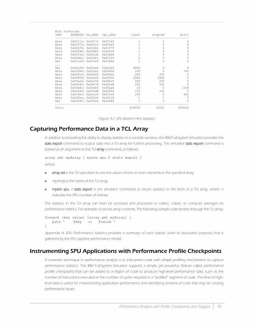
Figure 3-2. SPU Branch Hint Statistics

Capturing Performance Data in a TCL ArrayIn addition to providing the ability to display statistics in a console window, the IBM Full-System Simulator provides the

stats export command to output data into a Tcl array for further processing. The simulator stats export command is

passed as an argument to the Tcl array command, as follows:

array set myArray [ mysim spu 0 stats export ]

where:

array set is the Tcl operation to sets the values of one or more elements in the specified array.

myArray is the name of the Tcl array.

mysim spu n stats export is the simulator command to return statistics in the form of a Tcl array, where n

indicates the SPU number of interest.

The statistics in the Tcl array can then be accessed and processed to collect, collate, or compute averages on

performance metrics. For example, to access array contents, The following sample code iterates through the Tcl array:

foreach {key value} [array get myArray] {puts " $key => $value "

}

Appendix A, SPU Performance Statistics provides a summary of each statistic (with its associated purpose) that is

gathered by the SPU pipeline performance model.

Instrumenting SPU Applications with Performance Profile CheckpointsA common technique in performance analysis is to instrument code with simple profiling mechanisms to capture

performance statistics. The IBM Full-System Simulator supports a simple, yet powerful, feature called performance

profile checkpoints that can be added to a region of code to produce high-level performance data, such as the

number of instructions executed or the number of cycles required in a “profiled” segment of code. This kind of high-

level data is useful for characterizing application performance and identifying sections of code that may be causing

performance issues.

Hint historiesINST ADDRESS: br_addr tgt_addr count mispred stall-----------------------------------------------------------------------------hbra 0x0011c: 0x0017c 0x00140 1 1 0hbra 0x00374: 0x003c4 0x004e0 1 0 0hbra 0x01b74: 0x01b8c 0x01f78 1 0 0hbra 0x00088: 0x000b0 0x000c4 1 0 4hbra 0x0015c: 0x001dc 0x01bb8 1 0 0hbra 0x01bbc: 0x01d2c 0x02120 2 0 0hbr 0x021c0: 0x021e0 0x01bb8 1 0 5...hbr 0x00ef8: 0x00fa8 0x00340 9052 0 0hbra 0x00384: 0x003ac 0x00608 100 0 700hbra 0x00614: 0x0084c 0x006dc 200 200 0hbra 0x00904: 0x00a60 0x00930 2088 2088 0hbra 0x00ae4: 0x00c94 0x00b30 200 200 0hbra 0x00c9c: 0x00e78 0x00cd8 200 200 0hbra 0x00e8c: 0x00eb0 0x00aa8 24 0 1168hbra 0x00444: 0x004d8 0x00468 100 100 0hbrr 0x019ec: 0x01a14 0x019c8 100 0 400hbra 0x000ec: 0x00164 0x00128 1 1 0hbr 0x00240: 0x00264 0x00088 1 0 5-----------------------------------------------------------------------------Total 838508 12042 469242


Performance profile checkpoints are a simple mechanism for code instrumentation which can be used to delimit a

region of application code over which performance statistics are gathered by the IBM Full-System Simulator.

Performance profile checkpoints signal the simulator to display the current instruction and cycle counts for the SPU.

These can be used in pairs to determine the number of instructions executed and cycles consumed by a specific

region of SPU program code. This information can then be used to identify performance issues or quantify the

benefits of a potential optimization technique. Figure 3-3 illustrates how an SPU program can be instrumented with

performance profile checkpoints to obtain basic performance information about sections of the application code:

Figure 3-3. Performance Profile Checkpoint Instruction

A performance profile checkpoint is a special form of no-op instruction that the IBM Full-System Simulator interprets as

a request to display SPU performance data. This no-op instruction is a simple logical operation whose result has no

impact on program execution. There are 32 different no-op instructions that the IBM Full-System Simulator treats as

performance profile checkpoints.

When a checkpoint is encountered in program execution, the IBM Full-System Simulator prints a message with the

identity of the calling SPU and profiling data from that point in the program execution. These messages have the

form:

SPUn: CPm, xxxxx(yyyyy), zzzzzzz

where n is the SPU on which the performance profile checkpoint has been issued, m is the checkpoint number, xxxxx

is the instruction counter, yyyyy is the instruction count excluding no-ops, and zzzzzz is the cycle counter.

The application program interface (API) for the performance profile checkpoints is defined in the profile.h header file.

This file provides the C-language procedures, named prof_cp{n}() where n is a numeric value ranging from 0 to 31,

that generate the special no-op instructions. Special functions are assigned to the following performance profile

checkpoints:

prof_cp0() — clears the SPU pipeline performance statistics for this SPU. Can also be invoked with alias

prof_clear().

prof_cp30() — enables collection of SPU pipeline performance statistics for this SPU. Can also be invoked as

prof_start().

prof_cp31() — disables collection of SPU pipeline performance statistics for this SPU. Can also be invoked as

prof_stop().

The following sample code segment illustrates the checkpoint code that is added to code to clear, start, and stop

counters:

//declaration for checkpoint routine#include “profile.h”. . .prof_cp0(); // clear dataprof_cp30();// start recording data. . .<code_for_timing_metrics>. . .prof_cp31(); // stop recording data

Mambo simulation of SPU architecture

Application Software running on Mambo

instruction to Mambo simulator

simulation collects and outputs data

Display Window

SPU0: CP0, 204(193), 2408clear performance info

SPU0: CP30, 0(0), 0start recording performance info

SPU0: CP31, 203(192), 2656stop recording performance info

cmd_window

Host OS

16 Instrumenting SPU Applications with Performance Profile Checkpoints © IBM Corporation. All rights reserved.

A

ss

#include "profile.h". . .

prof_cp0(); // clear performance informationprof_cp30(); // start recording performance data. . .

<code_for_desired_timing_metrics>. . .prof_cp31(); // stop recording performance data

Enhancing Data Collection with TriggersIn the IBM Full-System Simulator, a trigger is a means of specifying a set of simulator commands that are to be

executed whenever a specific event occurs in the simulated system. To understand triggers, it is helpful to distinguish

between a trigger event and a trigger action. A trigger event is a specific event or state that can occur within the

simulated system that results in the execution of a user-defined TCL procedure called a trigger action. Trigger actions

can perform any number of simulator commands when the trigger event occurs. A common function performed by

the trigger action is to stop the simulation, using the simstop command, to allow user analysis of the state of the

system. If the trigger action does not stop the simulation, the simulator resumes execution when the trigger action

returns.

The IBM Full-System Simulator triggers are grouped into several classes based on trigger event type. Table 2-1

describes classes of triggers that are available.

Table 3-2. Classes of Triggers

Class Listing/Status Description

Global Associative trigger display assoc avail Machine-independent events

Machine Associative $sim trigger display assoc avail Machine-specific events

NOOP $sim trigger display assoc avail PPC NOP (“or x,x,x” where 10 <= x <= 31)

Console $sim trigger display console Console output string matching

System Memory $sim trigger display memory system list System memory access triggers (r, w, rw for EA or Rrange)

SPU Local Store $sim trigger display memory spu n list SPU local storage access triggers (r, w, rw for addrerange)

PPU PC Eff Addr $sim trigger display pc list PPU program counter EA trigger (“breakpoint”)

PPU PC Real Addr $sim trigger display real_pc list PPU program counter RA trigger (“breakpoint”)

SPU PC Addr $sim trigger display spu n pc list SPU program counter trigger (“breakpoint”)


Figure 3-4 illustrates how triggers are defined and used in the simulation environment:

Figure 3-4. Invoking a Trigger Procedure to Gather Performance Data

The numbered steps in Figure 3-4 outline how trigger actions and events are implemented in the IBM Full-System

Simulator:

1. The spu_start Tcl procedure, which specifies the trigger action, is defined in the Tcl interpreter. The input

arguments to the procedure provide information about the specific occurrence of the trigger event. These

arguments are typically formatted as one or more name-value pairs and are specific to the event type. Additional

input arguments can also be specified when the trigger is defined.

2. At any time during the simulation, the mysim trigger command can be used to set a trigger for a specific type of

event. The trigger command causes the IBM Full-System Simulator to associate a trigger action, defined by a Tcl

procedure, with a trigger event. In general, triggers are set from the command line as follows.

mysim trigger set trigger_type [trigger_event] [Tcl procedure_name]

where trigger_type defines the type of trigger that is being set, and trigger_event specifies the simulator-defined

event that initiates the trigger action (Table 3-2, “Classes of Triggers,” lists available event types of associative

triggers).

3. If the trigger event occurs in the execution of the application, the trigger action is executed by the Tcl interpreter.

4. For SPU events, the trigger action might execute the mysim spu 0 stats print command to print the SPU pipeline

statistics. Alternatively, these statistics can be captured in a Tcl array for further processing.

TCL INTERPRETER

Trigger Action: Defined by Tcl proc command:proc spu_start {args} {. . .computation_to_perform. . .}

A trigger action is registered with the Tcl interpreter, and controls what sequence of steps the simulator will perform when the trigger event occurs.

Trigger Event: Defined by a mysim trigger command: mysim trigger set assoc SPU_START spu_start

where the assoc SPU_START defines when the trigger action should be performed. Mambo monitors this association and calls the action if the event occurs.

% proc spu_start {args} { . . . }

% mysim trigger set assoc SPU_STARTspu_start***% mysim spu {spu_num} stats print. . .Total Cycle count 8576261. . .Total CPI 1.7. . .

[1]

[2]

[3]

[4]

spu_start is registered with interpreter

cmd_window

Application Software

Host OS

18 Enhancing Data Collection with Triggers © IBM Corporation. All rights reserved.

Associative triggers are a class of Tcl handlers that are associated with a set of predefined simulator events. The IBM

Full-System Simulator defines the following types of events that can be used with associative triggers:

The SPU_START, SPU_STOP, and SPU_PROF can be particularly useful in performance analysis of SPU applications.

The following trigger commands illustrate how associative triggers can be used to monitor SPU run status:

#--------- start SPU counter ---------proc spu_start {args} {

scan [lindex $args 0] " spu %d cycle %s" spunum cyclesputs "Start Counter: SPU $spunum started at $cycles cycles"

}

#--------- stop SPU counter ---------proc spu_stop {args} {

scan [lindex $args 0] " spu %d cycle %s" spunum cyclesputs "Stop Counter: SPU $spunum stopped at $cycles cycles"

}

where the spu_start and spu_stop trigger actions parse the input arguments and print a message indicating the

cycles at which an SPU is started and stopped. The format of argument 0 in the sample is similar to "{ spu 0 cycle

1000230 }".

SPU_PROF associative triggers can be used in conjunction with performance profile checkpoints to control when

and how performance data is collected during a simulation.

The command to set an associative trigger has the following fomat:

mysim trigger set assoc {trigger_event} {Tcl procedure_name}

.

The following commands, then, can be used to invoke the SPU counter triggers defined in the sample code above:

#--------- set triggers to monitor SPU run status ---------mysim trigger set assoc "SPU_START" spu_startmysim trigger set assoc "SPU_STOP" spu_stop

Tutorial: Collecting Performance Data with Checkpoints and TriggersThe tutorial in this section demonstrates how performance profile checkpoints and Mambo associative triggers can

be combined to collect performance information for a sample application.

Table 3-3. Event Types for Associative Triggers

Event Type a

a. To view a list of available event types for associative triggers, type mysim trigger display assoc avail at the simulation com-mand line.

Description

FATAL_ERROR Called on simulator fatal errors.

INTERNAL_ERROR Called on simulator internal errors.

SIM_START Called when the simulation starts (or resumes).

SIM_STOP Called when the simulation stops (or halts).

CALLTHRU Called when a PU-side application callthru is executed in the simulation.

SPU_STOP Called when an SPU stops (or halts) execution.

SPU_START Called when an SPU starts (or resumes) execution.

SPU_PROF Called when a prof_cp*() SPU-side profile checkpoint instruction is executed.


CONTEXT: A sample SPU program contains code for which cycle counts must be collected to analyze

performance metrics of specific computations. This code segment is contained within a loop that also

performs other computations that are not relevant to the desired SPU performance analysis. The

following pseudocode outlines the basis of this program:

for (i=1; i<loop_cnt; i++) {

< code that should not be included in performance statistics >

// Start of interesting code segment

< code for which performance statistics are desired >

// End of interesting code segment

< more code that should not be included in performance statistics >}

STRATEGY: A convenient approach of gathering performance measurements in this context is to combine

performance profile checkpoints and Mambo associative triggers for the SPU profiling events. In this

approach, profile checkpoints are added before the applicable code segment to reset and start

performance statistics collection, and then just following this code segment to indicate its end. An

associative trigger is set to aggregate total performance data from checkpoints across all iterations of

the loop.

STEP 1: Performance profile checkpoints are added to the application code around the relevant region of

code, as follows:

for (i=1; i<loop_cnt; i++){

< code that should not be included in performance statistics >

// Start of interesting code segmentprof_cp0(); // Reset performance statisticsprof_cp30(); // Start performance statistics collection. . .< code for which performance statistics are desired >. . .prof_cp31(); // Stop performance statistics and print// End of interesting code segment

< more code that should not be included in performance statistics >}

STEP 2: After instrumenting the application, a trigger action, spu_profile, is defined that accumulates the total

cycle count in the tot_cycles variable when the profile checkpoint at the end of the profiled region is

executed on an SPU:

proc spu_profile { args } {global tot_cyclesscan [lindex $args 0] " spu %d cycle %s rt %d " spunum cycles trignumif {$trignum == 31} {

set tot_cycles [expr $tot_cycles+$cycles]}

}

STEP 3: Prior to running the simulation, the following commands are used to associate the spu_profile trigger

action with SPU profile instruction events and initialize the tot_cycles variable:


mysim trigger set assoc SPU_PROF spu_profileset tot_cycles 0After running the simulation, the following TCL command is used to view the total cycle count:

puts "Total cycles for code segment is $tot_cycles”

The approach provided in this tutorial can be easily extended to collect any number of statistics that Mambo

maintains for SPU performance. For example, spu_profile can be extended as follows to collect single_cycle and

dual_cycle statistics for a code segment:

set tot_single_cycles 0set tot_dual_cycles 0

proc spu_profile { args } {global tot_single_cyclesglobal tot_dual_cyclesscan [lindex $args 0] " spu %d cycle %s rt %d " spunum cycles trignumif {$trignum == 31} {

array set stats [mysim spu $spunum stats export]set tot_single_cycles [expr $tot_single_cycles+$stats(single_cycle)]set tot_dual_cycles [expr $tot_dual_cycles+$stats(dual_cycle)]

}}

The same approach can be used to collect separate statistics on several code segments by using a different profile

checkpoint after each code segment. Based on the value in the $trignum variable, the spu_profile trigger action can

identify each segment of code and accumulate statistics into different variables for each code segment. Similarly, the

spu_profile trigger action can use the $spunum variable to determine which SPU has issued the profile checkpoint,

and then collect statistics by SPU or across all SPUs.


CHAPTER 4

Performance Data Collection and Analysiswith Emitters

This chapter introduces the IBM Full-System Simulator emitter framework, and providestutorial sections that demonstrate how to configure the simulator to emit event data, as wellas how to develop emitter readers to analyze the emitted event data. Topics in this chapterinclude:

Emitter Architecture Overview

Underlying Emitter Record Data Structure

Configuring Emitter Event Production

Tutorial: Configuring Emitter Event Production

Developing Emitter Readers to Process Event Data

Tutorial: Developing a Basic Emitter Reader


Emitter Architecture OverviewA key advantage of the IBM Full-System Simulator is its ability to collect multiple types of performance statistics at

varying levels of system granularity. Chapter 3, “Performance Analysis with Profile Checkpoints and Triggers”

introduced how performance profile checkpoints and triggers can be used to collect basic cycle count information

and summary statistics. To provide a more intensive level of performance data collection and measurement, the IBM

Full-System Simulator provides a modular emitter framework that decouples performance event collection from

performance analysis tools. The emitter framework provides a user-extensible and customizable event analysis system

that is comprised of two primary functional areas:

Event data production. Event data production comprises the instrumentation within the simulation environment

to detect events and produce emitter data. The simulator can identify a wide variety of architectural and

programmatic events that influence system and software performance. Using configuration commands, the

user can request the simulator to emit data for a specific set of events into a circular shared memory buffer.

Examples of these emitter events include instruction execution, memory references, and cache hits and misses.

Figure 4-1 lists the categories of events that are monitored by the simulator. The sti_emitter_data_t.h file

(available in the emitter directory of this release) defines all available event types and the data captured for each

event occurrence. It may be useful to review the declarations in this header file to determine the types of events

that can be monitored.

Event processing. Event processing comprises one or more emitter reader programs that access and analyze

emitter data. Analysis tasks generally include collecting and computing performance measurements and

statistics, visualizing program and system behavior, and capturing traces for post-processing. The IBM Full-System

Simulator is prepackaged with a set of pre-built sample emitter readers, and users can develop and customize

emitter readers based on performance metrics that are most relevant to their environment.

For enhanced usability, performance analysis is also provided by GUI-based emitter readers. These readers graph

memory access, cache misses, processor resource usage, and power usage as a function of time. Additionally, since

the emitter data stream includes the program counter, it is possible to trace interesting performance events (such as

high cache miss rates) back to a specific instruction of the simulated program or to specific lines of source code.

Figure 4-1. IBM Full-System Simulator Emitter Framework

Figure 4-1 provides a high-level overview of how the simulator processes events with emitter readers. At run-time, the

simulator writes emitter records in chronological order to the circular shared memory buffer based on user-specified

emitter controls. The simulator ensures that all attached emitter readers have accessed a record before overwriting

it—the simulator will halt further record production in the situation where the shared memory buffer is full and the

Hos

t OS

emitter reader 10

...

emitter record

emitter record

emitter record

emitter record

. . .

emitter record

emitter record

emitter record

emitter reader 1

Simulator emits data to memory buffer

magnified view of shared memory buffer

events deemed interesting to one or more emitter readers

emitter record

circular shared memory buffer

emitter record: EMIT_DATA

EMIT_DATA

Sim

ula

tor

Application running in the simulation


oldest record cannot be over-written. Emitter readers process the records in the shared memory buffer sequentially. If

data in an emitter record is “interesting,” the reader performs its computation or copies the data to an external

location; otherwise, it simply ignores records that are not of interest. Both processed and ignored records are marked

as having been accessed by the reader.

The emitter framework is entirely user-configurable. Users have the flexibility of enabling a large set of events to be

emitted and running several emitter readers simultaneously to process event data at the desired level of interest and

granularity.

The simulator supports call-thru functions that allow PU or SPU applications running in the simulator to generate

application-specific emitter records. In general, application-specific emitter records can be used to indicate the

occurrence of application-defined events or capture application-specific performance information.

Underlying Emitter Record Data StructureAn emitter record is the union of event data fields that describe properties of a simulation event. The IBM Full-System

Simulator implements an emitter record as a type of variant record, which enables multiple data types to be

combined into one dynamic data structure that occupies a single memory space. An emitter record consists of the

following components:

An EMIT_HEAD header whose structure is

common to all emitter records. The header

contains fields used to identify and handle the

emitter record, such as information about the

CPU, the event thread, an event serial

number, and a timestamp of when the

emitter record is created (i.e., the time the

event occurs.)

Event-specific data that is generated for a

simulator-monitored event type. The simulator

is designed to emit data for a number of event

types. If one of these event types occurs

during a simulation, the simulator determines whether record production has been enabled for the given event

type (via the simemit command), and constructs an emitter record containing the EMIT_HEAD data and the

event-specific information.

Configuring Emitter Event ProductionIn order to use an emitter reader, the simulation environment must first be configured to produce emitter data for the

reader to consume. The simulator provides commands to:

Specify the set of events that produce emitter data.

Table 4-1. Event Types Monitored by the IBM Full-System Simulator

Event Types

HEADER and FOOTERPU or SPU instructions

Cache accesses (hits or misses)

Process/thread state (create, kill, resume, etc)

TLB, SLB, ERAT operations

Device operations (disk)

Annotations

Transactions

head.cpu

head.thread

head.tag=sim.event.x

head.seqid

head.timestamp

Figure 4-2. Emitter Record Data Structure

sim.event.X such as a DMA.WRITE...IF “sim.event.X” enabled by simemitTHEN emit.sim.event.X to shared memory buffer

EMIT_HEAD fieldsEMIT_DATAEMIT_HEAD

25Performance Data Collection and Analysis with Emitters

Configure the number of emitter readers accessing records in the circular shared memory buffer.

Starting each emitter reader that is enabled during a simulation.

Specifying Events to Produce Emitter Data

The simemit command is a top-level command that specifies event types that should produce emitter data into the

shared memory buffer. The simemit command has the general form:

simemit set event_type boolean

which enables or disables the production of emitter records of the event type specified in event_type.

A separate simemit set command must be issued for the HEADER and

FOOTER records, as well as for each event type that a reader will monitor.

Not to be confused with the EMIT_HEAD record header, the HEADER

and FOOTER records are used by an emitter reader to track when it has

read every record in the shared memory buffer.

For example, the following simemit set commands can be used to

request emitter data for the “Instructions” and “APU_Instructions” events:

simemit set "Header_Record" 1simemit set "Footer_Record" 1simemit set "Instructions" 1simemit set "APU_Instructions" 1

Configuring the Number of Emitter Readers

The ereader command is a top-level command that controls emitter readers that are used in a simulation. The

ereader expect command specifies the number of emitter readers that will access the shared memory buffer during

the simulation. For example, the following command specifies that two emitter readers will be used in the simulation:

ereader expect 2

The simulator uses this number to ensure that all emitter readers have accessed an emitter record in the memory

buffer before it is overwritten by subsequent records.

Starting Emitter Readers

The ereader start command starts the specified emitter reader program. The general form of this command is:

ereader start reader_executable [pid] additional_args

where reader_executable is file name containing the emitter reader program, pid is the simulator process identifier

that the emitter reader will need to obtain access to the shared memory buffer, and additional_args are any

additional arguments that may be needed by the emitter reader program.

Tutorial: Configuring Emitter Event ProductionThe tutorial in this section describes how to configure the simulator to generate emitter records that will be used by

the emitter reader created in the “Developing a Basic Emitter Reader” tutorial.

CONTEXT: The emitter framework will be used to collect performance metrics for an SPU program. The IBM Full-

System Simulator must be configured to generate the emitter data needed for these measurements

and start the emitter reader.

NOTE By default, all events are disabled (set to 0). Also, input to the simemit command is case-sensitive.

sim.event.X

sim.event.Y

HEADER record

. . .FOOTER record

emitter reader

Figure 4-3. Header & Footer Records

emitter reader...

Shar

ed M

emor

y Bu

ffer

26 Configuring Emitter Event Production © IBM Corporation. All rights reserved.

STRATEGY: The commands to configure event production will be collected into a Tcl procedure to make it easier

to add emitter features to existing simulation scripts. This procedure includes the simemit set

commands to specify the emitter records to be generated and the ereader commands to configure

and start the emitter reader.

STEP 1: The emitter_start Tcl procedure contains the commands to configure event production and start the

sample reader. The procedure performs the following operations:

Specifies that Apu_Perf emitter records should be produced (in addition to the standard headerand footer records).

Specifies that one emitter reader will be consuming these records.

Starts the emitter reader program in the file named $env(EXEC_DIR)/../emitter/sti-annoperf.

proc emitter_start {} {global envsimemit set "Header_Record" 1simemit set "Footer_Record" 1simemit set "Apu_Perf" 1ereader expect 1puts "MAMBO PID is [pid]"

# Launch your emitter readerereader start $env(EXEC_DIR)/../emitter/sti-annoperf [pid]

}

STEP 2: This procedure can now be invoked as part of the simulation setup with the following commands:

# Set the appropriate exception to handle errorsif { [catch { emitter_start } errors] } { puts "EMITTER: No emitter support" puts " errors is $errors"} else { puts $errors }

The catch facility of Tcl is used to detect errors in starting the emitter reader that might otherwise go

undetected until later in the simulation, when these errors cannot be corrected without restarting the

simulation.

Developing Emitter Readers to Process Event DataUnlike simulator triggers that are generally used to execute a routine at regular intervals or at a particular cycle count,

emitter readers are able to collect and evaluate a wide array of detailed metrics about the PU or an SPU in the system

architecture. Multiple reader programs can simultaneously monitor emitter records, and perform the required

computations and analysis steps—each emitter reader acts only on emitter records that contain event tags that it is

monitoring. Emitter readers are developed to perform the following general types of analysis operations:

Calculate performance statistics. For example, an emitter reader can be used to compute the range, average,

standard deviation, or frequencies of execution times for the simulated application or code segment.

Visualize performance data for selected event occurrences. Through the stripstats_live utility, the IBM Full-System

Simulator provides an easy-to-use graphical frontend to the simulation engine. This utility is useful for configuring


parameters in order to visualize specific system and program behavior. Figure 4-4 shows a screen shot from

sample stripstats_live output:

Figure 4-4. Sample Stripstats_live Event Plot

Convert emitted event data to a trace format. The new trace information can be imported into existing analysis

tools. Multiple trace formats are supported simply by writing new emitter reader. The simulator itself does not

require any changes to support the additional formats.

Tutorial: Developing a Basic Emitter ReaderThe tutorial in this section demonstrates how to develop a sample emitter reader that analyzes the performance of a

simple SPU application. Developing emitter readers is a relatively simple task—an emitter reader is a C or C++ program

that accesses the emitter record in the memory buffer and processes emitted performance metrics. Figure 4-5

provides an activity diagram to illustrate the overall sequence of operations that are performed by an emitter reader.

Figure 4-5. Emitter Reader Activity Diagram

CONTEXT: The emitter framework is used to collect performance data for a simple SPU application that performs

the following DAXPY equation:

Initialize emitter reader program

Attach to shared memory buffer

using processor ID

Wait for expected readers to attach to

shared memory

Obtain a pointer to the next available

emitter record

Process emitter record according to

TAG type

Clean up and exit reader programIs footer

record?no yes

28 Developing Emitter Readers to Process Event Data © IBM Corporation. All rights reserved.

x = α * x + y

where x and y are double-precision n-vectors, and α is a scalar. An acronym for Double precision A

times X Plus Y, DAXPY is a Level 1 BLAS (Basic Linear Algebra Subprograms) operation that updates

vector x with the sum of a scaled vector x and vector y. Figure 4-6 illustrates the basic computation

performed by the SPU program:

Figure 4-6. DAXPY computation performed by the SPU program

The following code segment shows the main elements of the SPU program:

#include <fetch_incr.h>#include "profile.h"#include "apu_callthru.h"

int main(int spuid, addr64 argp, addr64 envp) {

/* Declarations and initialization */ . . .

prof_cp31();prof_cp0();for (i=0; i<my_len; i+=DMASIZE_ELEMENTS) {

vector double *xv = (vector double *) x_buf, *yv = (vector double *) y_buf;vector double av = spu_splats( cb.a );

/* DMA read segments of x and y into local storage */_read_mfc64((void *) x_buf , xp.ui[0], xp.ui[1], DMASIZE, tag, tid, rid);_read_mfc64((void *) y_buf , yp.ui[0], yp.ui[1], DMASIZE, tag, tid, rid);_set_mfc_tagmask(MFC_TAGID_TO_TAGMASK(tag));_wait_mfc_tags_all(); /* Wait for DMA to complete */

/* Perform the computation: x = a*x + y */prof_cp30();for (j=0; j<DMASIZE_QUADWORDS; j++) {

xv[j] = spu_madd(xv[j], av, yv[j]);}prof_cp31();

/* DMA write segment of x from local storage back to memory */_write_mfc64(xp.ui[0], xp.ui[1], (void *) x_buf, DMASIZE, tag, tid, rid);_set_mfc_tagmask(MFC_TAGID_TO_TAGMASK(tag));_wait_mfc_tags_all(); /* Wait for DMA to complete */

xp.ull += DMASIZE;yp.ull += DMASIZE;

}

= +α

yxx12

3

4

segments of DMA size


MamboSPUPerfStats();

/* Wrap-up operations*/. . .

This SPU application has been instrumented with performance profile checkpoints as described in

“Instrumenting SPU Applications with Performance Profile Checkpoints” on page 15. The section of the

code that performs the DAXPY computation is delimited with prof_cp30() and prof_cp31() calls to

restrict pipeline statistics collection to this region of the program. The call to MamboSPUPerfStats() is an

APU callthru defined in the “apu_callthru.h” header file. APU callthrus use no-op instructions to request

special processing by the simulator, much like the performance profile checkpoints.

MamboSPUPerfStats() produces an APU_PERF_STATS emitter record with the total cycle count. Apart

from the HEADER and FOOTER records, this single emitter record is the only record received by the

sample reader.

STRATEGY: The following sti-annoperf.cpp C++ sample reader is used to record cycle counts from the

APU_PERF_STATS records. Once this reader has accessed the FOOTER record (at the end of

simulation), it outputs the cycle counts it has captured for regions in the code.

STEP 1: The emitter program begins by declaring the necessary header files and initializing variables:

#define CONFIG_STI_EMITTER

extern "C" {#include "common/mambo.h"#include "emitter/emit_collector.h"#include <memory.h>}#include <map>#include <iostream>

using namespace std;

typedef map<const string, unsigned long long> RegionMap;typedef RegionMap::iterator RegionMapIter;typedef RegionMap::const_iterator RegionMapConstIter;

static RegionMap region_map;

EMITTER_CONTROLS eControl;int reader;

int main (int argc, char **argv) {int end = 0;int pid = 0;EMIT_DATA *ePtr = NULL;

printf("Reader Started\n");

if (argc < 2) {printf("ERROR: Usage: %s simulator-process-id\n", argv[0]);exit(-1);

}pid = atoi(argv[1]);

NOTE The alphaWorks releases of SystemSim for CBEA provide the full source code for this sample emitter reader in the emitter directory of the SDK installation path. This directory also contains source code for additional emitter readers.


STEP 2: The emitter reader is attached to the shared memory buffer using the processor identifier (PID):

reader = EMIT_AttachReader(pid, &eControl, 0, TRUE);if (reader == -1){

fprintf(stderr, "ERROR: Failed to attach reader\n");return(0);

}

STEP 3: This step performs the following program operations:

The emitter reader accesses the next record in the shared memory buffer (if necessary, waiting forthe simulator to produce a new record).

The reader determines if the record is of interest and increments the cycle count it isaccumulating.

The reader continues to access emitter records in the shared memory buffer until it encounters afooter tag, in which case the reader outputs the cycle count data and exits the program.

EMIT_ReadyWait(&eControl, reader, 1);string curr_region("Unspecified");

do {EMIT_AdvanceCurrent(&eControl, reader);ePtr = EMIT_CurrentEntry(&eControl, reader);switch (ePtr->header.head.tag)

{/** Emitter reader computation **/default:

/* Ignore */break;

}

if (ePtr->header.head.tag == TAG_FOOTER)end = 1;

}while (!end);

EMIT_Exit(&eControl, reader, TRUE);

// Dump the cycle counts per regionfor (RegionMapIter i = region_map.begin(); i != region_map.end(); ++i) {

cout << "Region: ’" << i->first << "’, Cycles: " << i->second << endl;

}

printf("Reader Terminating\n");

return(1);}

STEP 4: If a tag in the emitted record is an APU_PERF_STATS record, the emitter reader increments the cycle

count:

case TAG_APU_PERF_STATS:region_map[curr_region] += ePtr->perf_stats.cyc_count;break;

OUTPUT: Running the instrumented DAXPY program in concert with the sample reader produces output similar

to excerpted data provided below. Specific output lines are highlighted to identify cycle count


information or draw attention to output that is produced by specific emitter reader commands, such

as by the calls the reader is making to the reader API or as the result of the application call-thru

instructions (as described in the CONTEXT section of this tutorial).

. . .phdr[0] p_vaddr=0xc0, p_memsz=0x500, p_offset=0xc0, p_filesz=0x500Entry address: 0xc0Emitter Started: PID=25976Shared Memory Key is 103904Emitter Setup CompletedMAMBO PID is 25976Forking process for reader ’/home/.../sti-annoperf’Child is starting process ’/home/.../sti-annoperf’doneREADER: Shared Memory Key is 103904READER: Writer Data found at 0x40227000READER: Reader Data found at 0x40014000READER: Reader #0 attachedREADER(0): Reader Waiting for Header 1 in Emitter DataAll readers are attached. Checking if they are all ready...All ReadyREADER(0): Reader Found the Header in Emitter Datastop recording performance info.clear performance info.start recording performance info.. . .stop recording performance info.WARNING: 1846413: HALT ... program finished successfullyWARNING: 1846413: instruction count: 128099WARNING: 33048000000000: No processor activity for 3 secondsWARNING: 33048000000000: ... Stopping simulation33048000000000: ** Execution stopped: No activity in 3 secs, **33048000000000: ** finished running 0 instructions **READER: Emitter #0 exitingReader StartedRegion: ’Unspecified’, Cycles: 1798144Reader Terminating


APPENDIX A

SPU Performance Statistics

The IBM Full-System Simulator collects a number of statistics related to SPU performance. The following table lists statistics thatare available for this release:

Table A-1. SPU Statistics

Statistic Name (Rawstat Label) Semantic

performance_inst_count Instruction count (Profile checkpoint sensitive).

performance_cycle_count Cycle count (Profile checkpoint sensitive).

branch_taken Count of taken branch instructions (interpreter).

branch_not_taken Count of not-taken branches (interpreter).

hint_instructions Count of branch hint instructions.

hint_instruction_hits Count of times a hint instructions predicted correctly.

ls_contention Cycles in which LS RF access (ld/st insts) prevented prefetch.

sbi_contention Cycles in which SBI DMA operations prevented SPU LS access.

single_cycle Count of cycles in which an instruction was executed in only one pipeline.

dual_cycle Count of cycles in which an instruction was executed in both pipelines.

sp_issue_block Count of cycles dual issue was prevented due to inability to issue in tandem with an SP-class instruction.

dp_issue_block Count of cycles dual issue was prevented due to inability to issue in tandem with an DP-class instruction.

cross_issue_cycle Count of cycles in which issue pipe (0,1) sent an instruction to the opposite execution pipe (1,0).

nop_inst_count Number of NOP instructions executed (NOP, LNOP, HBR, and HBC).

src0_dep_cycle Cycles in which dual issue was prevented due to operand dependencies between the two instructions which were ready to issue simultaneously.

nop_cycle Count of cycles in which an NOP was executed in either pipeline.


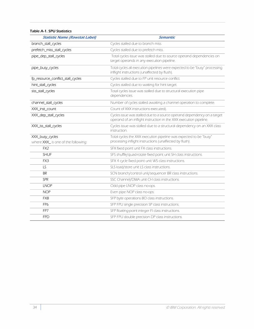
branch_stall_cycles Cycles stalled due to branch miss.

prefetch_miss_stall_cycles Cycles stalled due to prefetch miss.

pipe_dep_stall_cycles Total cycles issue was stalled due to source operand dependencies on target operands in any execution pipeline.

pipe_busy_cycles Total cycles all execution pipelines were expected to be “busy” processing inflight instructions (unaffected by flush).

fp_resource_conflict_stall_cycles Cycles stalled due to FP unit resource conflict.

hint_stall_cycles Cycles stalled due to waiting for hint target.

siss_stall_cycles Total cycles issue was stalled due to structural execution pipe dependencies.

channel_stall_cycles Number of cycles stalled awaiting a channel operation to complete.

XXX_inst_count Count of XXX instructions executed).

XXX_dep_stall_cycles Cycles issue was stalled due to a source operand dependency on a target operand of an inflight instruction in the XXX execution pipeline.

XXX_iss_stall_cycles Cycles issue was stalled due to a structural dependency on an XXX class instruction.

XXX_busy_cycles

where XXX_ is one of the following:

Total cycles the XXX execution pipeline was expected to be “busy” processing inflight instructions (unaffected by flush).

FX2 SFX fixed point unit FX class instructions.

SHUF SFS shuffle/quad-rotate fixed point unit SH class instructions.

FX3 SFX 4 cycle fixed point unit WS class instructions.

LS SLS load/store unit LS class instructions.

BR SCN branch/control unit/sequencer BR class instructions.

SPR SSC Channel/DMA unit CH class instructions.

LNOP Odd pipe LNOP class no-ops.

NOP Even pipe NOP class no-ops.

FXB SFP byte operations BO class instructions.

FP6 SFP FPU single precision SP class instructions.

FP7 SFP floating-point integer FI class instructions.

FPD SFP FPU double precision DP class instructions.

Table A-1. SPU Statistics

Statistic Name (Rawstat Label) Semantic


Performance Analysis with the IBM Full-System Simulator - iLab!

Documents

Transcript of Performance Analysis with the IBM Full-System Simulator - iLab!