Helsinki University of Technology Signal Processing LaboratoryTeknillinen korkeakoulu Signaalinkasittelytekniikan laboratorioEspoo 2007 Report 58

Performance Analysis of Multi-antenna and Multi-user Meth-ods for 3G and Beyond

Jyri Hamalainen

Dissertation for the degree of Doctor of Science in Technology to be pre-sented with due permission of the Department of Electrical and Communi-cations Engineering for public examination and debate in Auditorium S4 atHelsinki University of Technology (Espoo, Finland) on the 26th of January,2007, at 2 p.m.

Helsinki University of TechnologyDepartment of Electrical and Communications EngineeringSignal Processing Laboratory

Teknillinen korkeakouluSahko- ja tietoliikennetekniikan osastoSignaalinkasittelytekniikan laboratorio

Distribution:Helsinki University of TechnologySignal Processing LaboratoryP.O. Box 3000FIN-02015 HUTTel. +358-9-451 3211Fax. +358-9-452 3614E-mail: Mirja.Lemetyinen@hut.fi

c© Jyri Hamalainen

ISBN 978-951-22-8535-8 (Printed)ISBN 978-951-22-8536-5 (Electronic)ISSN 1458-6401

Otamedia OyEspoo 2007

Contents

1 Introduction 91.1 Transmit Diversity . . . . . . . . . . . . . . . . . . . . . . . . 91.2 Physical Layer Scheduling . . . . . . . . . . . . . . . . . . . . 111.3 Uplink MIMO . . . . . . . . . . . . . . . . . . . . . . . . . . . 121.4 Research Problems . . . . . . . . . . . . . . . . . . . . . . . . 131.5 Author’s Contribution and Other Work . . . . . . . . . . . . 14

2 UTRA Framework 152.1 UTRA FDD Downlink . . . . . . . . . . . . . . . . . . . . . . 152.2 High-Speed Downlink Packet Access . . . . . . . . . . . . . . 162.3 UTRA FDD Uplink . . . . . . . . . . . . . . . . . . . . . . . 182.4 Present Multi-antenna Methods in UTRA FDD . . . . . . . . 18

3 Closed-Loop Transmit Diversity 223.1 System Model, Algorithms and Performance Measures . . . . 233.2 Analysis Based on SNR Gain and Fading Figure . . . . . . . 293.3 Computation of Link Capacity . . . . . . . . . . . . . . . . . 393.4 Computation of BEP . . . . . . . . . . . . . . . . . . . . . . . 483.5 Effect of Feedback Errors . . . . . . . . . . . . . . . . . . . . 51

4 Physical Layer Scheduling on a Shared Link 574.1 System Model . . . . . . . . . . . . . . . . . . . . . . . . . . . 584.2 Round Robin Scheduling with TSC . . . . . . . . . . . . . . . 624.3 On-off Scheduling with TSC . . . . . . . . . . . . . . . . . . . 644.4 Maximum SNR Scheduling with TSC . . . . . . . . . . . . . 694.5 Comparisons and Conclusions . . . . . . . . . . . . . . . . . . 704.6 Computation of Bit Error Probabilities . . . . . . . . . . . . . 734.7 Effect of Quantization . . . . . . . . . . . . . . . . . . . . . . 78

5 Scheduling for UTRA FDD Uplink 855.1 System Model . . . . . . . . . . . . . . . . . . . . . . . . . . . 855.2 Analysis of Transmit Power . . . . . . . . . . . . . . . . . . . 875.3 OOS Gain in WCDMA Uplink . . . . . . . . . . . . . . . . . 915.4 Performance Results and Conclusions . . . . . . . . . . . . . 94

6 MIMO in UTRA FDD Uplink 1006.1 MIMO Algorithms . . . . . . . . . . . . . . . . . . . . . . . . 1006.2 Uplink Load Equations . . . . . . . . . . . . . . . . . . . . . . 1036.3 Performance Comparisons . . . . . . . . . . . . . . . . . . . . 106

7 Conclusions 112

Abstract

Performance of cellular networks has become an issue with forecasted grow-ing public demand for medium and high data rate services. Motivatedby these expectations multi-antenna techniques such as transmit diver-sity (TD), channel-aware scheduling and multiple-input multiple-output(MIMO) transceivers have received a lot of enthusiasm within wireless com-munications community.

We first focus on closed-loop (CL) TD and introduce extended mode1 and 2 (e-mode 1 and 2) algorithms that are designed based on universalterrestrial radio access (UTRA) frequency division duplex (FDD) CL mode 1and 2. We derive analytical performance results for e-mode 1 and 2 in termsof signal to noise ratio (SNR) gain, link capacity and bit error probability(BEP). We also consider the effect of feedback errors to the performance ofclosed-loop system.

In the analysis of channel-aware scheduling we focus on on-off schedul-ing (OOS) where user’s feedback consists of only a single bit. Performanceresults in both downlink and uplink clearly indicate that most of the achiev-able gain from channel-aware scheduling can be obtained with very scarcechannel state information (CSI). Results also show that the design of feed-back channel is of great importance because feedback errors may seriouslydegrade the system performance.

The third topic of the thesis concentrates on MIMO techniques thatcan be implemented in UTRA FDD uplink without major revisions to thecurrent air interface. We show that the UTRA FDD uplink coverage and ca-pacity performance can be boosted by single-input multiple-output (SIMO)and MIMO transceivers. The information MIMO employing parallel mul-tiplexing instead of transmit diversity shows its potential when extremelyhigh user data rates are needed.

Tiivistelma

Solukkoverkkojen suorituskyky on noussut tarkeaan rooliin nopeiden data-palveluiden kasvuennusteiden myota. Naiden kasvuodotusten perusteellamoniantennitekniikat kuten lahetysdiversiteetti, kanavan huomioon otta-va lahetyksen aikataulutus seka useaa samanaikaista datavirtaa tukevatlahetinvastaanotinmenetelmat ovat saaneet osakseen paljon kiinnostustalangattoman tietoliikenteen tutkijayhteisossa.

Tutkimuksessa keskitytaan aluksi suljettua saatoa kayttaviinlahetysdiversiteettimenetelmiin, missa yhteydessa esitellaan laajen-netut moodien 1 ja 2 algoritmit, jotka on aiemmin kehitetty kolmannensukupolven WCDMA jarjestelman suljetun saadon moodien 1 ja 2 poh-jalta. Laajennetuille moodien 1 ja 2 algoritmeille johdetaan analyyttisiasuorituskykytuloksia kayttaen mittarina signaali-kohinasuhteen paran-nusta, linkin kapasiteettia seka bittivirheiden todennakoisyytta. Myossaatovirheiden vaikutusta jarjestelman suorituskykyyn tarkastellaan.

Lahetyksen aikataulutuksen analyysi painottuu kytkettyyn aikataulu-tukseen, missa kayttajan saatoinformaatio sisaltyy yhteen bittiin. Sekayla- etta alalinkin suorituskykytulokset osoittavat selvasti, etta suurin osamahdollisesta parannuksesta voidaan saavuttaa hyvin karkeaan kanavati-lan informaatioon perustuen. Tulokset osoittavat myos, etta saatokanavansuunnittelu on tarkeaa, koska saatovirheet voivat vakavasti heikentaajarjestelman suorituskykya.

Kolmannessa aihealueessa keskitytaan moniantennitekniikoihin, jotkavoidaan toteuttaa WCDMA jarjestelman ylalinkissa ilman perustavanlaa-tuisia muutoksia nykyiseen ilmarajapintaan. Tutkimuksessa osoitetaan, ettaylalinkin peittoa ja kapasiteettia voidaan parantaa tutkituilla monianten-nitekniikoilla olipa lahettimessa yksi tai useampia antenneja. Menetelma,jossa informaatio jaetaan useisiin rinnakkaisiin datavirtoihin sen sijaan ettakaytettaisiin vain yhta datavirtaa, osoittautuu erityisen lupaavaksi kuntarvitaan hyvin nopeita tiedonsiirtoyhteyksia.

Preface

This thesis is based on the work that was carried out in the NokiaNetworks/Strategy and Technology and Helsinki University of Technol-ogy/Signal Processing Laboratory.

I want to express my deepest gratitude to Professor Risto Wichmanwith who we have had many interesting journeys through various researchsubjects.

I wish to thank Associated Professor Mohamed-Slim Alouini and Pro-fessor Tapani Ristaniemi for refereeing this thesis.

I am grateful to my colleagues at Nokia for cooperation and discussions.I highly appreciate the open and supporting atmosphere in our team thatcontains many world-class experts of radio communications.

I also wish to thank Professor Visa Koivunen for partly financing mywork in Signal Processing Laboratory.

I am indebted to my father, Emeritus Professor Rauno Hamalainen forgiving me basic understanding about the fundamental nature of science.

Finally, I wish to thank very deeply my wife Seija, and my childrenRimma and Leevi for all the patience and understanding they have shown.

Oulu, December 18, 2006 Jyri Hamalainen

Abbreviations

3G 3rd Generation3GPP 3rd Generation partnership project (produces WCDMA standard)ACK Positive acknowledgementARQ Automatic repeat requestAS Angular spreadAWGN Additional white Gaussian noiseBEP Bit error probabilityBF Beam-formingBPSK Binary phase shift keyingBS Base stationCCH Control channelCDF Cumulative distribution functionCDMA Code division multiple accessCL Closed-loopCPICH Common pilot channelCQI Channel quality informationCSI Channel state informationDCH Data channelDoA Direction of arrivalDPCCH Dedicated physical control channelDPCH Dedicated physical channelDPDCH Dedicated physical data channele-mode 1 Extended mode 1e-mode 2 Extended mode 2FBF Fixed beam-formingFBI Feedback information (in UTRA FDD)FDD Frequency division duplexFTP File transfer protocolGPS Global positioning systemGSM Global system for mobile communicationsHARQ Hybrid automatic repeat requestHS-DSCH High speed downlink shared channelHSDPA High speed downlink packet accessIC Interference cancellationIP Internet protocolITU International telecommunications unionMAI Multiple access interferenceMbps Mega bits per secondMcps Mega chips per secondMIMO Multiple-input multiple-outputMISO Multiple-input single-outputMMSE Minimum mean square error

MRC Maximal ratio combiningNACK Negative acknowledgementOL Open-loopOOS On-off schedulingPC Power controlP-CPICH Primary common pilot channelPDF Probability density functionPIC Parallel interference cancellationQAM Quadrature amplitude modulationQoS Quality of serviceQPSK Quadrature phase shift keyingRACH Random access channelRLB Radio link budgetS-CPICH Secondary common pilot channelSIC Serial interference cancellationSIMO Single-input multiple-outputSINR Signal to interference and noise ratioSISO Single input single outputSNR Signal to noise ratioSTBC Space-time block codeSTTD Space-time transmit diversityTD Transmit diversityTFCI Transport format combination indicatorTPC Transmit power control (in UTRA FDD)TSC Transmitter selection combiningTTI Transport time intervalUSBF User specific beam-formingUTRA Universal Terrestrial radio accessWCDMA Wideband CDMAWLAN Wireless local area network

1 Introduction

The purpose of this thesis is to summarize the research work that the authorcarried out during 2000-2005 in Nokia Networks/Strategy and Technologyand Helsinki University of Technology/Signal Processing Laboratory. Sincethe third generation (3G) universal terrestrial radio access (UTRA) fre-quency division duplex (FDD), referred to as wideband code division multi-ple access (WCDMA), has fueled the research, it has been natural to adoptthe corresponding system framework as a starting point. We shortly recallthis framework in Section 2.

Nevertheless, since the results of this thesis are obtained by employinggeneric models and analytical tools, they are not limited to 3G systemsonly. Research topics have closely followed the interests of industry contain-ing transmit diversity (TD), physical layer scheduling and multiple-inputmultiple-output (MIMO). In the following we briefly introduce these topicsand list the publications that have been used as a basis for the thesis. De-tailed discussion is placed on Sections 3 - 6 containing a more extensive listof references.

1.1 Transmit Diversity

Multiantenna transceivers have great potential to improve the performanceof wireless systems. Compared to wireline systems, the inferior capacity ofwireless cellular systems is caused by several different physical constraintslike co-channel and adjacent channel interference, channel propagation loss,and flat or multi-path fading channels. Multi-antenna transmission andreception techniques are currently seen as one of the most promising ap-proaches for significantly increasing the coverage, capacity and spectral ef-ficiency of wireless systems.

Traditionally, multi-antenna techniques have mainly been consideredwithin base stations (BS), because deploying multiple antennas in the userterminal is not straightforward due to cost, complexity of signal processing,and power consumption. Diversity reception, for example, is a mature tech-nology and it has been successfully applied in base stations to increase cellcoverage. Another well-known technique is the beamforming (BF) wherehighly correlated BS antennas are used. In beamforming, downlink beamis formed using the direction of arrival (DoA) information that is estimatedbased on uplink measurements. Such estimates can be carried out also in fre-quency division duplex (FDD) systems when the difference between uplinkand downlink frequencies is small with respect to the carrier frequency.

Conventional BF is attractive if BS antennas are placed well above therooftop level where angular spread (AS) of the received radio signal is usuallysmall. If BS antennas are placed below the rooftop level or angular spreadis large due to some other reason, the efficient use of conventional BF may

become difficult since uncertainty of user DoA increases and there might beseveral strong DoAs corresponding to different signal paths.

In contrast to beamforming, for transmit diversity techniques rich scat-tering environment is advantageous and most of the TD methods assumefrom the beginning that transmit antenna correlation is low. It is usual todivide TD techniques into two basic classes, namely into closed-loop (CL)methods, where short term channel state information (CSI) is available inthe transmitter, and into open-loop (OL) methods where such informationdoes not exist but, on the other hand, some space-time processing is usedin order to improve the radio performance. Nevertheless, this classificationis artificial because there exist also hybrid methods where both short-termCSI and OL space-time processing is applied.

With CL techniques, quantized CSI is transmitted to the BS via a controlchannel. The side information can then be used to weight the transmittedsignals such that they combine constructively in the antennas of mobilestation increasing the received signal power and consequently range andcapacity. In case of uncorrelated signal paths, CL TD techniques can providediversity benefit and increase the signal to noise ratio (SNR) in the receiver.When uplink and downlink operate in different frequency bands the sideinformation related to the downlink channel requires additional signaling,and the design of signaling formats optimizing some performance measure inthe mobile terminal while simultaneously minimizing the amount of uplinksignaling makes the problem challenging.

Besides CL methods, several different OL TD diversity techniques basedon space-time coding have been developed intensively in recent years, andthe simplest space-time block code, referred to as space-time transmit di-versity (STTD), has been adopted into UTRA FDD as an OL transmitdiversity method for two transmit antennas. Space-time codes are blind inthe sense that they do not exploit CSI in the transmitter. The codes areable to provide diversity gain but no antenna gain, and the diversity gaindecreases as a function of correlation between the antenna elements.

Closed-loop techniques typically outperform the OL ones particularlywithin low-mobility environments where the delay of the feedback signalingdoes not exceed channel coherence time. The short-term CSI in the trans-mitter requires a control channel from the receiver to the transmitter anddesign of different quantization strategies is an important task. One of thegoals of this thesis is to analyze the relation between feedback quantizationand system performance for CL methods similar to UTRA FDD CL modes.Contrary to conventional BF the CL algorithms do not require accuratecalibration of the transmit antennas. Only coarse calibration of antennaelements is necessary in order to avoid spurious antenna gain patterns andunexpected interference to the network.

Transmit diversity is considered in Section 3 where we introduce andanalyze various CL methods. The main reference publications by the author

10

are [1] - [6] but useful information can be obtained also in [7] - [16].

1.2 Physical Layer Scheduling

Besides multi-antenna methods, also multi-user methods such as physicallayer scheduling can be efficiently used in order to increase the system effi-ciency. When the transmission is not delay constrained, spectral efficiencyof multi-user systems can be increased by employing shared channels andchannel-aware schedulers, which divide the resources between multiple users.Such shared channels are already used in cdma2000 1xEV-DO and WCDMAhigh speed downlink packet access (HSDPA).

Efficient use of shared channels greatly depends on the available CSIin the transmitter. It is known that in case of single input single output(SISO) channel the capacity of the shared link can be maximized by giving allresources to the user with the strongest channel. When uplink and downlinkemploy different frequency bands as in WCDMA mode, scheduling requiresa separate feedback channel, which may generate a lot of interference in theuplink. Furthermore, the capacity of control channels is necessarily limited,and large amounts of control information imply large latencies in feedbacksignaling, which limits the operation range of the system to slow mobilevelocities.

In Section 4 we investigate this feedback problem by assuming a heavilyquantized channel quality information (CQI). We consider a downlink on-offscheduling (OOS) where users report with one bit, whether their receivedSNRs fall below or above a predefined threshold. The scheduler then ran-domly picks one of the users above the threshold and transmits to the userwith all available power. We compare OOS to round robin and maximumSNR schedulers that provide lower and upper bounds to the performanceof OOS. Capacity gains of the three schedulers are derived together withtransmitter selection combining (TSC) and Shannon capacity is used as aperformance measure. Besides the shared channel capacity we also considerthe bit-error-probability (BEP) of individual users in the presence of heavilyquantized CQI. An important goal in Section 4 is to find out the effect offeedback errors.

With increasing load in the network, the uplink may also become a ca-pacity bottleneck, and there is an increasing demand to improve coverageand throughput in the uplink as well. Feasibility study of UTRA FDD up-link enhancements introduces similar mechanisms as with HSDPA. On thecontrary to HSDPA, uplink data and control channels employ fast transmitpower control (PC), which is inherent characteristic of CDMA uplink. Accu-rate fast transmit PC is mandatory, because otherwise users in the vicinityof the base station would completely mask intra-cell users on cell edges.

Channel-aware scheduling improves the system performance also in up-link, but to this end the BS transmitter must somehow acquire channel state

11

information from different users. Thus, even if a user does not transmit anydata in the dedicated data channel, it has to transmit some control infor-mation so that the scheduler is able to measure the channel state. Strictquality of service requirements are applied on continuously transmitted con-trol channel, and therefore scheduling can be only applied on the dedicatedchannel. Scheduling may increase the system efficiency if the total numberof users in the system is larger than the number of transmitting users, i.e.there are backlogged users waiting in the queue for transmission and thescheduler allows users with strongest channels to transmit. However, thelarger is the number of users in the system the larger is the overhead causedby users’ control channels. Thus, the increased interference due to con-trol signaling and decreased interference due to scheduling should be jointlyconsidered in algorithm design.

In Section 5 we study the effect of OOS to the required transmit powerwhen PC is on. On-off scheduling is compared to two reference systems.The first one applies discontinuous transmission on data channel but thescheduler does not take into account channel state information. The secondreference system transmits continuously on data and control channels. Wewill show that control channel overhead may limit the performance of OOSalthough users could tolerate unbounded delays.

Section 4 is based on articles [17] - [19] while references [20] - [24] provideadditional information. Discussion on the uplink scheduling of Section 5 ismainly adopted from [25].

1.3 Uplink MIMO

Multiple degrees of freedom offered by multiple transmit and receive anten-nas can be used for diversity or for spatial multiplexing. In the former case,a single data stream is transmitted and multiple antennas are used to de-crease the variance of the received signal and thereby improve the quality ofthe radio link. In the latter case, multiple transceiver antennas are used forparallel multiplexing, i.e. to transmit several data streams simultaneouslyto a user to increase peak data rates. In Section 6, these two approacheswill be referred to as diversity MIMO and information MIMO, respectively.

In terms of channel capacity, information MIMO is a much more im-pressive concept than diversity MIMO. It is known that with parallel mul-tiplexing, the capacity increases linearly with the number of transmit andreceive antennas when the number of transmit antennas equals the numberof receive antennas and when the channels between the antennas are inde-pendent and identically distributed. This observation has stimulated largeinterest toward MIMO transceivers, and in addition to academic researchMIMO is actively being studied in standardization fora of different wirelesssystems, like UTRA, IEEE 802.11n and IEEE 802.16e.

The first release of UTRA FDD was completed in 1999. At that time, re-

12

search on information MIMO techniques was at initial stage, but the releasealready specified two-antenna open-loop and closed-loop transmit diversitymodes that are part of the most recent Release 6 as well1. With multiple re-ceive antennas these modes form basis for diversity MIMO. The introductionof more advanced MIMO techniques to WCDMA has not been straightfor-ward. A lot of standardization effort in 3GPP has been dedicated to extendthe specification of diversity MIMO to more than two transmit antennas,and information MIMO techniques to HSDPA have been extensively stud-ied as well. However, at the time of writing no MIMO techniques have beenaccepted to technical specifications yet.

The basic idea of MIMO is useful in both downlink and uplink of acellular system. Recently, the discussion has mainly focused on downlinkbecause it is expected that capacity demanding services will be first appliedin downlink. Nevertheless, the introduction of new services such as video-phones will make it extremely important to reach high spectral efficiencyalso in the uplink direction. In Section 6 we consider two simple MIMOapproaches that are suitable for UTRA FDD uplink. Discussion is basedon [26] - [29].

1.4 Research Problems

The first goal of this thesis is to model and analyze some closed-loop transmitdiversity methods that are of practical interest. We note that if quantizedfeedback is assumed in closed-loop transmit diversity the distribution of thesum channel SNR becomes cumbersome to compute in most cases. Thereforeit is important to find suitable means in order to circumvent this difficultyand carry out closed-form analysis. Thus, the main research problems are:

• Develop analytical tools by which closed-loop transmit diversity meth-ods can be analyzed.

• Carry out the analysis of the studied methods by using the developedtools and appropriate performance measures.

Channel-aware schedulers in FDD systems require fast feedback fromreceiver. In order to keep the signaling overhead as small as possible it isattractive to use heavy channel feedback quantisation. In such systems itis of great importance to find the impact of quantization to the schedulerperformance. Also system specific aspects should be carefully considered.Main research questions in connection with physical layer scheduling are:

• Analyze the impact of channel feedback quantization. What is the per-formance of multi-user scheduling when channel feedback is minimizedversus the systems with ideal feedback and no feedback?

1Recently, the second closed-loop mode was removed from Release’5 onwards in thecampaign of simplifying the specifications

13

• Model and determine the effect of system specific aspects like feedbackerrors and increased control overhead.

The benefits of uplink MIMO in practical systems need to be charac-terized. For that purpose the UTRA FDD uplink provides an interestingframework. Research problems are:

• Determine simple and practical way to deploy MIMO in UTRA FDDuplink.

• Investigate the system level gain of uplink MIMO in UTRA FDDsystem.

1.5 Author’s Contribution and Other Work

Publications have been coauthored in close cooperation and decomposingthe publications into separate parts contributed by different authors is notfeasible. Author’s contribution to the publications [1] - [13], [15] - [21], [25] -[28] has been essential in general, and he has assumed the main responsibilityin deriving mathematical analysis. In [26] - [28] simulations were carriedout by Esa Tiirola (Nokia Networks), Kari Pajukoski (Nokia Networks) andMarkku Kuusela (Nokia Research Center).

It is well acknowledged that the performance of various multi-antennatechniques depends on the assumed channel model. Therefore developmentand analysis of channel models is an important task. While this task is notin the focus of this thesis we only note that the author of the thesis hasrecently made some publications on this topic [30] - [34].

14

2 UTRA Framework

In WCDMA, narrowband user information is spread over a wide bandwidthby modulating a low-rate user data sequence with a high-rate spreadingcode (channelization code). The length of the spreading codes varies from 4to 512 chips (in the uplink the maximum code length is 256 chips) and thechip rate is 3.84 Mcps (Mega chips per second) which together with transmitpulse shape filter leads to the carrier bandwidth of approximately 5 MHz.Variable spreading factors and multi-code transmission are used in order tosupport a wide scale of different data rates [35].

Scrambling codes of length 38400 chips are employed on top of chan-nelization codes. In the downlink channelization codes are used to separatedifferent intra-cell users and separation of inter-cell users is based on differentscrambling codes. In the uplink the scrambling codes separate different usersand channelization codes separate different physical data and control chan-nels of a user [36]. This difference between the code usage in the downlinkand uplink is essential: The limited number of orthogonal channelizationcodes imposes a strict upper bound to the achievable downlink capacityunless information MIMO technique reusing the channelization codes areused. The limitation is not strict in the uplink, because one user may use allchannelization codes and the set of long scrambling codes contains severalmillions of codes.

The basic UTRA FDD mode supports user data rates up to 2.3 Mbpsboth in uplink and downlink. In downlink, transmission on the peak datarate requires the usage of 3 parallel channelization codes with spreadingfactor 4 which allocates 75% of code resources to a single user [37]. Inuplink, terminal transmitting with the peak data rate is seen as a largeinterference source in the network but available code resources of other intra-cell users are not affected. High peak-to-average ratio of multi-code signalssets stringent requirements to transmitters, which are particularly criticalto mobile stations.

2.1 UTRA FDD Downlink

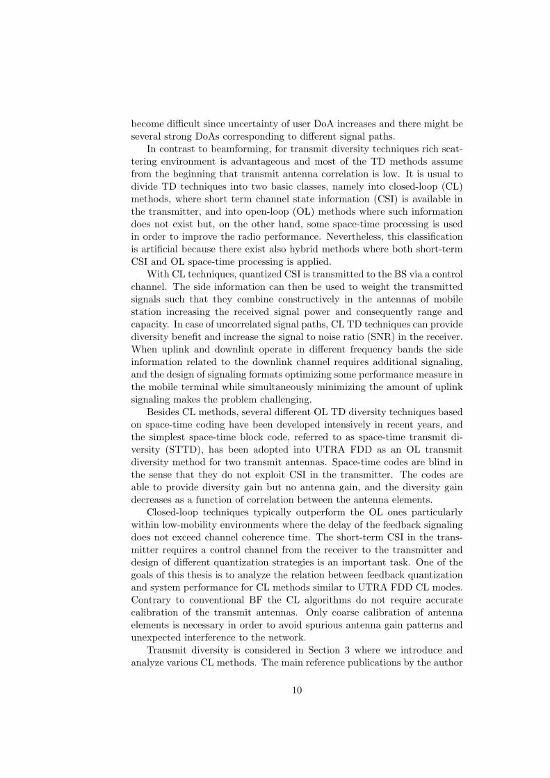
Figure 1 presents a simplified downlink channel and frame structure. Eachframe is divided into 15 time slots the frame length being 10 ms. The radioframe carries a dedicated physical channel (DPCH) that further divides intodedicated physical data channel (DPDCH) and dedicated physical controlchannel (DPCCH). The control channel contains transmit power control(TPC) bits for fast power control, transport format combination indicator(TFCI) bits that inform the receiver which transport channels are activeand pilot bits enabling the channel and signal to interference and noise ratio(SINR) estimation from DPCH [38].

Figure 1 further shows the primary common pilot channel (P-CPICH)

15

Figure 1: Downlink frame structure for dedicated physical channel.

and the secondary common pilot channel (S-CPICH) without time slot struc-ture, where the numbers in brackets indicate the numbers of different pilotchannels. While receiver may estimate the channel from the dedicated chan-nel, better result is usually obtained when employing P-CPICH or S-CPICH,because these common pilot channels, especially P-CPICH, have highertransmit power. In practice, P-CPICH usually takes approximately 10%of transmit power resources of the base station while power on S-CPICHsis lower. This high transmit power on P-CPICH is due to the fact that P-CPICH is always transmitted to the whole cell enabling handover and cellselection/reselection measurements. By adjusting power differences betweenP-CPICHs of adjacent cells the network load can be balanced. The poweron S-CPICH can be lower because it has to cover only part of the cell [38].Usually S-CPICH is applied in connection with beamforming.

According to the present UTRA FDD specification only two P-CPICHsare available at maximum while multiple S-CPICHs can be introduced, forexample, for beamforming purposes. This introduces a serious backwardcompatibility problem for the design of multi-antenna algorithms with morethan two transmit antennas. If the power in P-CPICH is kept fixed but thepower is divided to more than two transmit antennas, the channel estimationin legacy mobile terminals is deteriorated. If the power of P-CPICH isincreased, interference to network increases as well.

2.2 High-Speed Downlink Packet Access

Starting from Release 5, WCDMA contains a highly optimized downlinkdata transmission concept referred to as high speed downlink packet access(HSDPA) [39], [40]. The HSDPA concept applies several advanced physicallayer solutions, listed below, to enable high throughput and reduced servicedelays. The HSDPA concept introduces a new type of transport channel,referred to as the high speed downlink shared channel (HS-DSCH), with afixed spreading factor of length 16. In addition, HSDPA utilizes

• adaptive modulation and coding (link adaptation)

16

• high order modulation

• hybrid automatic repeat request (HARQ) solution

• reduced length (2 ms) transport time interval (TTI)

• fast cell selection (FCS)

• physical layer scheduler located in base station

The control of HS-DSCH is terminated in the base station in order toadapt rapidly to changing channel conditions. Adaptation rate is increasedby shortening transport time interval (TTI) from 10 ms in Release ’99 andRelease 4 to 2 ms. The same TTI can be used to transmit with multiplechannelization codes to the same user depending on terminal capability. Inaddition, it is possible to multiplex multiple users in the code domain withinone HS-DSCH TTI.

Link adaptation is implemented with a large set of possible transportformat combinations, each associated with a unique combination of modu-lation, coding and block size parameters. Release ’99 and Release 4 supportonly QPSK modulation, but an HSDPA terminal also supports 16-QAM.This increases the peak data rates in good channel conditions. Fast powercontrol, which aims to keep the received signal to interference and noiseratio (SINR) constant, is not applied. This is because with non-real timedata transmission it is more efficient to allow the received SINR to vary andchange modulation and coding according to the channel state. Furthermore,fast power control used together with a high data rate and high power trans-port channel would generate large interference peaks to neighboring cells.

Data rates are assigned to a user based on CQI that is measured at theterminal and signalled to the base station in the form of a channel qualityindicator. Thus, CQI feedback provides the necessary information for effi-cient real-time link adaptation and this enables a form of multi-user diversitywhen applied together with physical layer scheduling. It is known that inSISO scenario, throughput is maximized by maximum SNR scheduler trans-mitting to the user that reports the best SNR to the base station [41], [42].Yet, when the distances of the users from the serving base station are dif-ferent, such a scheduler is not fair, because the users on cell edge rarely getany transmission. Therefore, different fair schedulers have been developed,which aim to equalize transmission periods among the users. The physicallayer scheduling mechanism is part of the WCDMA HSDPA specificationbut its implementation is vendor specific option. Instead of SNR, it is alsopossible to signal data rates or capacities by mapping the SNR values ap-propriately.

Fast cell selection is used to select the transmitting base station fromthe set of active base stations. Hybrid ARQ combines retransmission with

17

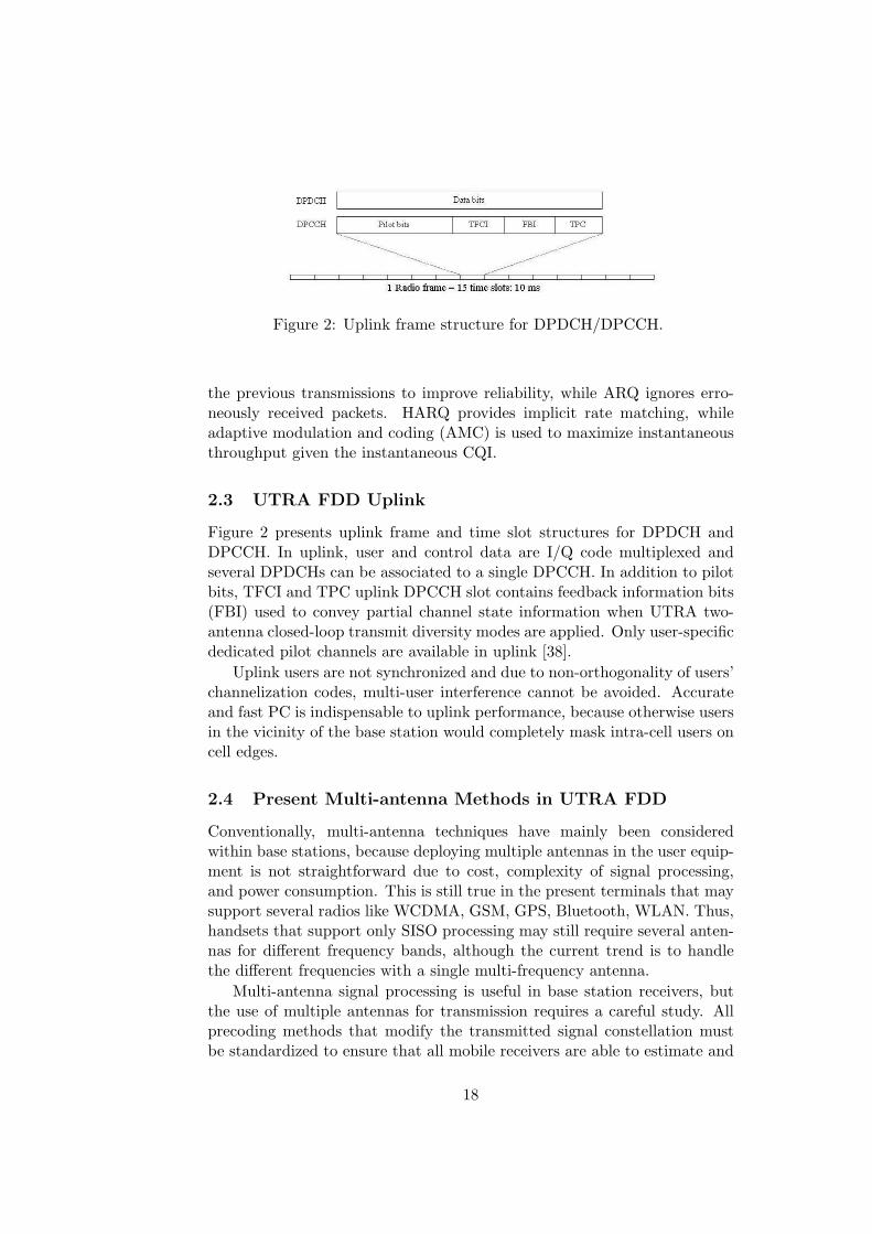
Figure 2: Uplink frame structure for DPDCH/DPCCH.

the previous transmissions to improve reliability, while ARQ ignores erro-neously received packets. HARQ provides implicit rate matching, whileadaptive modulation and coding (AMC) is used to maximize instantaneousthroughput given the instantaneous CQI.

2.3 UTRA FDD Uplink

Figure 2 presents uplink frame and time slot structures for DPDCH andDPCCH. In uplink, user and control data are I/Q code multiplexed andseveral DPDCHs can be associated to a single DPCCH. In addition to pilotbits, TFCI and TPC uplink DPCCH slot contains feedback information bits(FBI) used to convey partial channel state information when UTRA two-antenna closed-loop transmit diversity modes are applied. Only user-specificdedicated pilot channels are available in uplink [38].

Uplink users are not synchronized and due to non-orthogonality of users’channelization codes, multi-user interference cannot be avoided. Accurateand fast PC is indispensable to uplink performance, because otherwise usersin the vicinity of the base station would completely mask intra-cell users oncell edges.

2.4 Present Multi-antenna Methods in UTRA FDD

Conventionally, multi-antenna techniques have mainly been consideredwithin base stations, because deploying multiple antennas in the user equip-ment is not straightforward due to cost, complexity of signal processing,and power consumption. This is still true in the present terminals that maysupport several radios like WCDMA, GSM, GPS, Bluetooth, WLAN. Thus,handsets that support only SISO processing may still require several anten-nas for different frequency bands, although the current trend is to handlethe different frequencies with a single multi-frequency antenna.

Multi-antenna signal processing is useful in base station receivers, butthe use of multiple antennas for transmission requires a careful study. Allprecoding methods that modify the transmitted signal constellation mustbe standardized to ensure that all mobile receivers are able to estimate and

18

detect the signals from different antennas. An extensive standardizationprocess has been required even in case of transmit beamforming.

Present UTRA FDD specification supports two-antenna transmit diver-sity and transmit beamforming. Such multiple input single output (MISO)systems for downlink have been intensively studied, because at the timewhen the 3rd generation partnership project (3GPP) standardization wasinitiated most scenarios predicted that the capacity of wireless networkswould be limited by the downlink connection. Although diversity MISOdoes not promise as high peak data rates as information MIMO, transmitdiversity improves fading resistance and beamforming increases the systemcapacity while its impact to individual user data rates is small. InformationMIMO techniques are not included in the UTRA FDD specification, mostlybecause the initial standardization work was carried out during the 1990’swhen the development of practical information MIMO algorithms was stillin the beginning.

Conventional transmit beamforming provides the simplest approach toincrease system capacity and coverage in downlink. The current 3GPP spec-ification supports both fixed beamforming (FBF) and user specific beam-forming (USBF) modes in downlink. Fixed beamforming introduces addi-tional sectors to the cell, because the short term variation of the beams issmall and a handover between the beams is required for mobile users. Eachbeam is associated with a unique S-CPICH while P-CPICH is transmittedto the whole cell.

Fixed beamforming is able to relax the code limitation in downlink,because orthogonal spreading codes can be reused within the same cell dueto spatial filtering. It is also possible to use different scrambling codes indifferent beams. In the presence of flat fading the channelization codes ofdifferent users within the same beam remain orthogonal, because they arescrambled with the same code. Different beams interfere with each other andincrease intra-cell interference, but when angular spread (AS) is reasonablysmall as in macro-cells, this interference remains acceptable. In addition tolarger interference levels, control signaling overhead increases due to inter-beam handovers, because logically the fixed beams behave in the same wayas different sectors in base stations. The overall effect to system capacity ispositive though, and according to [43], a 2.4-fold system capacity gain canbe achieved with a four-element antenna array when compared to a singleantenna cell.

Instead of fixed transmit beams, USBF generates individual beams toeach user. More sophisticated signal processing algorithms can be used, andconsequently, USBF is able to provide higher individual data rates thanFBF. In practice, USBF cannot be utilized in most cases within UTRAFDD downlink, because it prevents the user from employing the P-CPICHas a phase reference and according to the current specification S-CPICHcannot be employed in individual beams. Thus, channel estimation must

19

be based on dedicated pilot channels whose transmit power is low whichmay seriously corrupt channel estimation in terminal. Then only high datarate users near the base station may take full advantage from USBF. User-specific beamforming is optional for terminals in HS-DSCH and thereforenetwork cannot assume that all users are able to support it.

Downlink beamforming changes the statistics of the fading signal, andin environments with small angular spread array gain dominates diversitygain. Therefore, the estimation of downlink beamforming gain over singleantenna transmission is rather straightforward: The gain is approximatelythe same as the array gain. In uplink this is not as simple, though.

In uplink, both UTRA FDD beamforming techniques can be imple-mented in a straightforward manner in the receiver. The simplest ap-proach is to combine the selected signal paths using maximal ratio com-bining (MRC) in the beam space. This leads to a standard Rake-receiverconcept. The most challenging practical problems are related to beam selec-tion (DoA estimation in USBF) and cost-efficient receiver structures. Theformer problem is related to the large variety of physical environments withdifferent channel profiles. Furthermore, mobile’s transmit power is typicallylow for low data rate connections making the channel estimation difficult.The latter problem arises from the fact that baseband complexity increasesrapidly when spatio-temporal estimation processes are introduced. For ex-ample, preambles of random access channel (RACH) need to be monitoredsimultaneously for each beam in order to avoid additional delays in connec-tion setup time.

Transmit beamforming improves the downlink capacity in UTRA FDD,but it is important to notice that receive beamforming is not necessarily thebest solution in uplink because of its lack of diversity gain [44]. This givesrise to a trade-off between uplink and downlink design targets. If downlinkcapacity is the bottleneck, FBF provides a good solution in macro-cells. Onthe other hand, if good uplink coverage is the primary target, uncorrelatedantennas with suitable receiver algorithms provide a better solution.

According to [44] basic receive diversity solution outperforms receivebeamforming performance even when angular spread is small. Moreover,transmit beamforming in downlink looses its good performance in terms ofcapacity and coverage when AS becomes large so that beams cannot beaccurately pointed to users any more. Hence, there is a need for a multi-antenna transmission method in downlink that performs well when correla-tion between the transmit antennas is low. In general, low correlation can beachieved when the distance between antenna elements in base station is sev-eral wavelengths. Conventional beamforming algorithms do not apply anymore, and to this end, several open-loop transmit diversity techniques havebeen developed in recent years. The simplest space-time block code [45], hasbeen adopted into 3GPP specification as a two-antenna open-loop transmitdiversity method.

20

Space–time codes provide diversity reducing the variance of the receivedsignal which further translates into reduced transmit power in downlink.However, space–time codes do not increase the received SNR when com-pared to single antenna transmission. With uncorrelated transmit antennasreceived SNR can be improved when short-term CSI is made available in thetransmitter. Until Release 4 UTRA FDD technical specifications containedtwo closed-loop modes [46] where the relative phase and power between thetwo transmit antennas were adjusted according to feedback information bitssignaled from mobile to a base station through a dedicated control channel.Later releases contain only the closed-loop mode in which relative phase be-tween two transmit antennas is adjusted and both antennas transmit withthe same power.

UTRA FDD supports two P-CPICHs in order to enable efficient channelestimation of the two channels when transmit diversity is in use. In case ofclosed-loop modes, feedback commands are determined from the P-CPICHsand transmit weights are applied on dedicated traffic channels. Commonpilots are transmitted with higher power than dedicated pilots and there-fore common pilots should be used for channel estimation whenever possible.With closed-loop modes, dedicated pilots are used for the verification of thetransmit weights (feedback commands may be erroneously decoded in thebase station and the mobile cannot automatically assume that the transmit-ter uses the weights that the mobile has instructed) and channel estimatescan still be calculated from P-CPICHs.

The discussion on transmit diversity extensions to more than two trans-mit antenna systems was active in 3GPP for a long time [47]. The mainconcern was that the benefits from additional transmit antennas may notjustify the additional complexity of transceiver and system design. A diffi-cult backward compatibility with former releases is also encountered if thetransmit power of common pilot channels is divided between, say, four trans-mit antennas to support channel estimation in mobile receivers. Then legacyterminals that are able to receive only two pilot channels loose performance,because they loose half of the available power of the common pilot signals.At the time of writing, proposed extensions of transmit diversity techniqueshave been withdrawn and the focus has been shifted to the specification ofinformation MIMO techniques.

21

3 Closed-Loop Transmit Diversity

Beginning from [45], [48] and [49] a huge amount of papers on open-looptransmit diversity methods such as space-time block and trellis codes havebeen published. At the same time the number of publications that focus onclosed-loop methods with partial CSI has been smaller. It seems that onlytransmit antenna selection is widely studied in the literature. For closed-loop methods with partial CSI a good quantization is needed which leadsto a difficult problem that usually allows only numerical solutions. Thisproblem makes the general analysis of closed-loop methods very difficult.

In spite of above-mentioned problem the analysis of closed-loop methodscan be carried out in some interesting and practically viable cases. Besidesthe well-known transmit antenna selection we introduce and analyze twobasic types of suboptimal closed-loop transmit diversity methods. The de-sign of these methods is motivated by the UTRA FDD closed-loop transmitdiversity mode 1 and 2. Therefore we will call them in the following asextended mode 1 (e-mode 1) and extended mode 2 (e-mode 2).

After introducing the system model in Section 3.1 we represent SNRgain analysis of e-mode 1 and 2 in Section 3.2. The content of Section 3.2is based on [1], [2] and [3] while [7], [9] and [12] provide some additionalinformation. Previously, SNR gain analysis for some closed-loop methodswas also represented in [50] and [51].

The capacity analysis of Section 3.3 relies on [6], see also [11]. Previously,a generic capacity analysis for methods with CSI at the transmitter has beengiven in [53] while [54] provides explicit capacity formulas in case of receiverselection combining and MRC. As such the results in [54] can be also used forthe analysis of transmitter selection combining and orthogonal space-timeblock codes.

Method for the BEP computation in Section 3.4 is due [5]. Also [55], [56]and [57] represent similar results in terms of bit error probability but [55]provides mainly simulation results, [56] assumes delayed ideal feedback whileanalysis of [57] focuses on corrupted feedback. The effect of feedback biterrors is considered in Section 3.5 based on results of [4]. The effect offeedback errors has also been studied in [15] where the site selection diversitytransmission is investigated and in [57] where feedback system model isdifferent from the model used in [4].

Finally, we note that also the effect of channel polarization to the perfor-mance of TD can be studied as is done in [14] where the performance of somesimple TD techniques was considered assuming a channel model which takesinto account the channel polarization [30]. Besides the conventional OL TDmethods of [14], polarization matching (or polarization steering) has beeninvestigated [10]. In polarization matching base station employs the infor-mation concerning the uplink channel polarization when selecting downlinktransmit weights. This method was demonstrated in [59] and [60] showing

22

that the polarization matching can be feasible in mobile environments.

3.1 System Model, Algorithms and Performance Measures

System model for the CL TD methods is given in Figure 3. We denoteby Mt the number of transmit antennas and by L we refer to the numberof channel paths. Corresponding impulse responses are denoted by hm,l,where l is the channel path number and m defines the channel betweenmth transmit and receive antenna. It is assumed that impulse responses areuncorrelated complex zero-mean Gaussian. If Mt or L is 1 we simply neglectthe corresponding index.

Signal Model

We have only a single receive antenna in the mobile and the columns hm ofchannel matrix H consist of channel taps hm,l. in the presence of closed-looptransmit diversity the received signal in the mobile station is of the form

r = (Hw)s + n,

where s is the transmitted symbol, n contains zero-mean Gaussian noisesamples and w ∈ CMt consists of complex transmit weights such that ‖w‖ =1. We assume that the channel matrix H is perfectly known in the receiver.In UTRA FDD two-antenna CL modes H is estimated from P-CPICH andtransmit weights are applied on DPDCH or HS-DSCH.

Provided that quantized set W of feedback weights is given, the selectionof the most suitable transmit weight vector w can be based on the receivedSNR, i.e. we solve the problem

Find w ∈ W : ‖Hw‖ = maxw∈W

‖Hw‖. (1)

Instead of SNR other measures such as channel capacity or bit-error ratecould be used. However, SNR provides the simplest practical measure.

Instead of defining an explicit quantization scheme as in (1), CSI feed-back can be modelled statistically, giving rise to mean feedback and covari-ance feedback schemes [58]. With mean feedback the transmitter assumesthat the channel coefficients are distributed according to multivariate com-plex Gaussian distribution N(w, δ2I), where w and δ2 can be interpreted asthe estimate of the channel based on the feedback and the variance of theestimate, respectively. In covariance feedback, the channel (known at thetransmitter) is distributed as N(0,R). This can be interpreted to model acase where the channel is changing very rapidly and the mean feedback isunable to track or model the instantaneous channel dynamics. However, thegeometrical properties of the channel change slowly, and it is in many casesrealistic to assume that the transmitter may know the channel covariancematrix R.

23

Figure 3: General system structure for CL TD.

In WCDMA, quantization of CSI is coarse and the capacity of the finite-rate feedback channel is defined explicitly. Thus, in this context it is morenatural to study deterministic feedback strategies and characterize theirperformance given the number of quantization bits.

Feedback Channel

We begin by noticing that in the forthcoming discussion we will use ’feedbackword’ and ’transmit weight’ interchangeably. In practice they are not thesame but there is a one-to-one mapping between the quantization set andthe set of feedback words.

Fundamental issues of control channels carrying short-term channel in-formation are the very strict time delay and control overhead limits as wellas the high robustness requirements. The use of strong error-correctingcodes on the feedback channel is not a favorable solution, because codingincreases signaling overhead and system may become complex, because theshort-term feedback information needs to be decoded within a very shorttime frame. In the analysis of transmit diversity methods we assume a simi-lar feedback channel structure as with the UTRA FDD closed-loop transmitdiversity modes, where uncoded control information is transmitted to BSat each TTI in a dedicated control channel. Fast PC is applied to theuplink control channel so that the control information is received with ap-proximately constant SNR and feedback bit errors can be assumed to beuniformly distributed in time. Hence, fast PC increases the robustness, be-cause error bursts can be avoided and probability of feedback bit errors canbe controlled with a proper transmit power.

Finally, we note that the effect of feedback latency is neglected in thisstudy, which is approximately valid within low mobility environments. Theeffect of feedback delay to the performance of closed-loop transmit diversityis studied in [8], [56], [57] and [61].

24

Feedback Algorithms

With a given quantization (1) defines the weight that maximizes the SNRin the set of all weight vectors. When the number of antennas is smallthis approach can be viable, but in general case such an exhaustive searchis not a good solution because computational complexity in mobile stationis growing exponentially with respect to the number of transmit antennas.Furthermore, since feedback capacity is usually strictly limited, it is advan-tageous if feedback words can be divided flexibly into independent subwordsthat can be used in the transmitter before the whole feedback word is re-ceived. If continuous feedback update is not possible, then either feedbackdelay is long — which means that algorithm is sensitive to mobile speed —or the required feedback capacity is high.

Keeping in mind the problems above we introduce three suboptimal al-gorithms. First we introduce the well-known selection algorithm

Transmitter Selection Combining (TSC). In this case the set of trans-mit weights consists of vectors w = (0, . . . , 0, 1, 0, . . . , 0), where the nonzerocomponent indicates the best channel in terms of received SNR. Hence

‖Hw‖ = max‖hm‖ : 1 ≤ m ≤ Mt.

Since the quantization set has Mt points, dlog2(Mt)e feedback bits areneeded. TSC is very simple and it requires a low feedback capacity butlater on we will see that its performance is not very good and it is sensitiveto feedback errors.

As another example of a suboptimal algorithm we introduce extendedmode 1 in which only the relative phases between signals from separateantennas are adjusted. This special form of the co-phasing algorithm hasbeen addressed previously in [50], where it was assumed that a feedbackword of length Mt−1 bits is provided to the base station having Mt antennaelements. Thus, the feedback word consists of information about the stateof each relative phase between reference antenna and other Mt−1 antennas.A generalization utilizing Nrp feedback bits/relative phase is given by thefollowing algorithm.

Extended Mode 1 (e-mode 1). Here feedback bits are selected antennawise using the condition

‖h1 + vmhm‖ = max‖h1 + vmhm‖ : vm = ej2π(n−1)/2Nrp, 1 ≤ n ≤ 2Nrp.

The components of the final transmit weight w are of the form

wm =1√Mt

1, m = 1,

vm, m > 1.

25

That is, each phase is adjusted independently against the phase of the firstchannel. It should be noticed that the complexity of the example algorithmincreases linearly with additional antennas, i.e., complexity is proportionalto (Mt− 1)2Nrp . The feedback word in e-mode 1 can be divided into Mt− 1subwords which all can be used independently in the transmitter. Thereforethe required feedback overhead is not very high and computational work inmobile terminal can be spread to a longer time interval. We also note thatsince e-mode 1 applies only phase adjustments, the transmit antennas canmaintain power balance which is advantageous in some practical systems.

A natural generalization to the above scheme is to weight transmit am-plitudes in addition to adjusting phase differences. Intuitively, the strongerthe channel, the more power should be transmitted through it. Bearingthis in mind we give the following more feedback scheme, which provides ageneralization for e-mode 1.

Extended Mode 2 (e-mode 2). In this algorithm receiver ranks someor all ‖hm‖Mt

m=1 and selects the phase feedback by applying e-mode 1.Order and phase difference information is signaled to the transmitter whichthen chooses appropriate amplitude and phase weights from a finite set oftransmit weights.

A crucial question when applying e-mode 2 is the selection of a suitablequantizer. This problem will be studied in detail in Section 3.2. Here weonly briefly note that uniform quantizer suffices for the quantization of thephase differences, but finding a good quantizer for transmit powers is notany more a trivial task. If the number of transmit antennas is small thenthe quantization for amplitude weights can be found using simulations butwhen the number of transmit antennas is large, it can become a cumbersometask.

The length of the feedback word in e-mode 2 depends on the design, butif full order information is signaled, then at least dlog2(Mt!)e order bits areneeded in addition to (Mt−1)Nrp phase bits. The design that uses separatesubwords corresponding to each antenna requires Mtdlog2(Mt)e order bits.

We remark that when Mt = 2 and Nrp = 2 e-mode 1 resembles UTRAFDD closed-loop transmit diversity mode 1. The only difference betweenUTRA mode 1 and e-mode 1 is that in UTRA mode 1 the feedback wordresults from the interpolation between two consecutive one–bit feedbackwords. However, the difference is irrelevant here because feedback delay isnot taken into account. Similarly, when Mt = 2 and Nrp = 3 e-mode 2coincides with UTRA closed-loop transmit diversity mode 2.

Both e-modes are clearly suboptimal and their performance could be im-proved without changing the quantization by determining the feedback wordjointly across transmit antennas instead of independently for each transmitantenna. However, derivation of analytical results for joint quantization

26

when M > 2 becomes significantly more involved that with independentquantization. Furthermore, joint quantization would make the computa-tional complexity exponential with respect to the number of transmit anten-nas. Another approach to reduce the computational complexity is to updatefeedback word iteratively exploiting the memory of the fading channel, andrestrict the search of a new transmit weight vector to the neighborhood of thecurrent weight [62]. The performance of such a scheme depends intimatelyon the fading rate of the channel and feedback delay which complicates theanalysis.

In addition to independent quantization of transmit weights with respectto a reference antenna, e-mode is suboptimal, because amplitude and phasedifference of transmit weights are adjusted independently, which is similarto polar quantization [103]. In [63, 64], a design criterion for quantizationis developed that is based on the minimization of maximum correlation be-tween the codewords. Codebooks for different number of transmit antennasand feedback bits are then determined by computer search given the designcriterion. In these codebooks, amplitude and phase are quantized jointly.

Codebooks developed in [63, 64] do not facilitate continuous update offeedback word, because bits in the feedback words do not correspond di-rectly to transmit antennas. On the other hand, without feedback latencyand feedback errors, performance of the codebooks [63, 64] is necessary bet-ter than that of the suboptimal e-modes — provided that the computersearch resulted in a good codebook. However, in practical wireless commu-nication systems differences between the two approaches are small, becausethe number of codewords and the number of transmit antennas is limited.

SNR Gain and Fading Figure

The performance of various diversity methods is usually studied by usingexpected receiver bit-error probability or link capacity as a measure. Besidesthese approaches the computation of expected SNR in the receiver provides asimple and useful indicator that illustrates the benefit of closed-loop transmitdiversity. This is based on the fact that SNR gain provides informationconcerning the coherent combining, or beamforming, benefit inherent tosuccessful closed-loop processing of the transmitted signal. We define theSNR gain simply by

G = E‖Hw‖2, ‖w‖ = 1, E‖hm‖2 = 1, (2)

where w is the transmit weight vector defined by the feedback algorithm.At this stage we introduce notations

γm = ‖hm‖2, z = ‖Hw‖2 (3)

that will be found useful later. We note that the former notation of (3) isapplied only when the scaling in (2) is valid.

27

By using Schwarz inequality we find that

G ≤ E‖H‖2 · ‖w‖2 = Mt. (4)

Hence, maximum achievable SNR gain is given by the number of transmitantennas. On the other hand, if feedback information is not available andtransmit weights are randomly selected, then there is no coherent combininggain and G = 1. In flat Rayleigh fading channel the bound (4) is obtainedby ideal feedback wm = hm/‖H‖.

The drawback of SNR gain is that it does not indicate the diversitybenefit that can be better illustrated through the fading figure defined by

F =G2

E(‖Hw‖2 − G)2 =G2

E‖Hw‖4 − G2(5)

that takes into account also the second moment of SNR. For a flat Rayleighfading channel F = 1. When a closed-loop transmit diversity method isused the value of the fading figure becomes larger than one indicating thedecrease in signal variation. If the variation of the signal power is fullycompensated, then the channel seen by the receiver is static and F = ∞.

Figure 4 displays the received SNR as a function of time for SISO andeight-antenna MISO with ideal feedback. It is found that besides the SNRgain the signal variation is remarkably reduced in case of closed-loop MISO.The 90% probability thresholds for SNRs are plotted using dashed lineswhile the expected SNRs are expressed using solid lines.

Link Capacity

Link capacity is probably the most popular analytical performance measure.In Section 3.3 we focus on two cases. First we consider the channel capacityin the presence of constant transmit power and receiver CSI only. Thencapacity is of the form

Cora(γ) = B · Elog2(1 + γz), (6)

where B [Hz] is the channel bandwidth, γ is the mean SNR and z refers tothe instantaneous received SNR [52], [53]. This expression is also referredto as average channel capacity [52], because it is obtained by averagingover the channel states. In case of closed-loop transmit diversity methodsz = ‖Hw‖2.

Capacity (6) is a suitable performance measure in HSDPA where powercontrol is not applied on shared channel. In dedicated data channels fastpower control aims to invert the channel and a more appropriate perfor-mance measure is given by the capacity

Ccifr(γ) = B · log2

(1 + γ/E1/z

)(7)

that is valid when transmitter adapts its power to maintain a constant SNRat the receiver and fixed coding and modulation is applied [53].

28

1 1.5 2 2.510

−2

10−1

100

101

Time [s]

SN

R

90% Power level

Mean signal power

SNR gain

Single antenna system

Eight−antenna system

Figure 4: Received SNR for SISO (lower curve) and eight-antenna MISO(upper curve) with ideal feedback. Dashed lines: 90% level of SNR. Solidlines: mean SNR. Single path Rayleigh fading channel is assumed.

Bit-Error Probability (BEP)

The SNR gain and fading figure are valuable relative measures for the linkperformance and capacity gives good fundamental performance information.The BEP, however, provides a concrete and practical performance measurethat can be directly used in system design. In general, BEP is defined by

Pe(γ) = EPmod(γ · z), (8)

where Pmod is the error rate of the applied modulation in terms of receivedSNR. Similarly with the capacity this approach leads to very difficult equa-tions when certain feedback algorithms are studied. In Section 3.4 we deducean asymptotic formula for (8) in two-antenna case and provide an accurateapproximation that is valid in the whole SNR scale.

3.2 Analysis Based on SNR Gain and Fading Figure

In the analysis we first compute the SNR gain for e-mode 1 and 2. Duringthe analysis we deduce an amplitude weight quantization for e-mode 2 that isbased on the order information. After showing general results that are validin case Mt > 1 we give an extended analysis in two-antenna case. With thislimitation the computation of fading figure is simplified and, on the otherhand, we are able to extend the analysis to the case of multi-path fading.Besides the SNR gain computation we show that amplitude quantization for

29

e-mode 2 does not depend on the temporal channel profile as long as channeltaps are uncorrelated complex zero-mean Gaussian.

Analysis of SNR Gain in Flat Rayleigh Fading

The simplest example of a closed-loop algorithm is provided by TSC. Sincewe use the performance of this algorithm as a baseline reference we recallthat SNR for TSC is given by

G =Mt∑

m=1

1m

.

This formula is known already from [65] and it indicates that SNR gain ofthe TSC against the single antenna system is proportional to log(Mt) forlarge Mt.

The main benefit of TSC is the small feedback overhead requirement thatmakes it attractive from practical implementation point of view. The maindrawbacks of TCS are the poor performance - when compared against moresophisticated closed-loop algorithms - and sensitivity to feedback errors [4].

The computation of SNR gain for e-mode 1 and 2 can be carried outfollowing [1] and [2]. We note that SNR gain for e-mode 1 in case Nrp = 1was also given in [50]. Since e-mode 1 is a special case of e-mode 2 weconsider first e-mode 2. Then we can write Hw = Hu, where u consists ofreal amplitude weights and H contains channel coefficients after the phaseadjustments. The expectation of the received SNR in the mobile is now ofthe form

Ez = uT EHHHu = uTRfbu, (9)

where Rfb is the covariance matrix corresponding to the adjusted channels.Hence, the use of short-term feedback introduces beneficial long-term corre-lation. The elements of Rfb are given by

(Rfb)m,k = ReE√γmγk · ejψm,k = E√γmγkRe

Eejψm,k, (10)

where ψm,k = φm−φk is the difference between mth and kth adjusted phases.If there are (Mt − 1)Nrp phase bits available, then φ1 = 0 and φm, m > 1,is uniformly distributed on (−π/2Nrp , π/2Nrp). In (10) the second equalityholds because phase and order information are applied independently andphase and amplitude of a zero-mean Gaussian variable are uncorrelated. Letus compute the latter expectation. If m > 1 we have

Ecosψm,1 =2Nrp−1

π

∫ π/2Nrp

−π/2Nrp

cosψ dψ =2Nrp

πsin

( π

2Nrp

)=: cNrp . (11)

The expectation for cosψm,k, m, k > 1, m 6= k is computed by applying theidentity ψm,k = ψm,1 − ψk,1 and cosine summation formula. Since ψm,1 and

30

ψk,1 are independent if m 6= k we obtain

Ecosψm,k = Ecosψm,1Ecosψk,1 = c2Nrp

. (12)

In case of e-mode 1 there is only phase information available and we setum = 1/

√Mt. Furthermore, since amplitudes are uncorrelated and follow

Rayleigh distribution, there holds

E√γmγk = E√γmE√γk =π

4, m 6= k. (13)

After combining (10)-(13) we find that

(Rfb)m,m = 1, (Rfb)m,1 = (Rfb)1,m =πcNrp

4, m > 1,

(Rfb)m,k = (Rfb)k,m =πc2

Nrp

4, m 6= k, k 6= 1.

(14)

The SNR gain of e-mode 1 is obtained by using elements (14) in (9). Aftersome elementary manipulations it is found that

G = 1 +Mt − 12Mt

(1 +

Mt − 22

· cNrp

)· πcNrp . (15)

Hence, in contrast to TSC the SNR gain grows linearly with respect to thenumber of antennas. In the presence of ideal phasing information in thetransmitter we have

c∞ = limNrp→∞

cNrp = 1.

Then the upper bound for the SNR gain due to the phasing is given by

G = 1 +π

4(Mt − 1).

Figure 5 shows the SNR gain for e-mode 1 and TSC in terms of the numberof transmit antennas. The results show that most of the achievable SNRgain from phase adjustments is obtained when Nrp = 3. Antenna selectionis clearly inferior to e-mode 1 when Nrp > 1 but if Nrp = 1 there is not muchdifference in performance provided that the number of transmit antennas issmall.

If order information is available in the transmitter we indicate it bybrackets around the channel index. Then γ(m) ≥ γ(k) if m > k and equa-tion (13) is not valid any more because ordered amplitudes are not uncor-related. By using (10)-(12) we find that

(Rfb)m,k = E√γ(m)γ(k)εm,k = %m,kεm,k,

where %m,k is a correlation due to the order statistics and εm,k = cNrp ifk = 1 or m = 1 and εm,k = c2

Nrpotherwise. Phasing and ordering together

31

1 2 3 4 5 6 7 80

1

2

3

4

5

6

7

8

9

Number of transmit antennas

SN

R g

ain

[dB

]

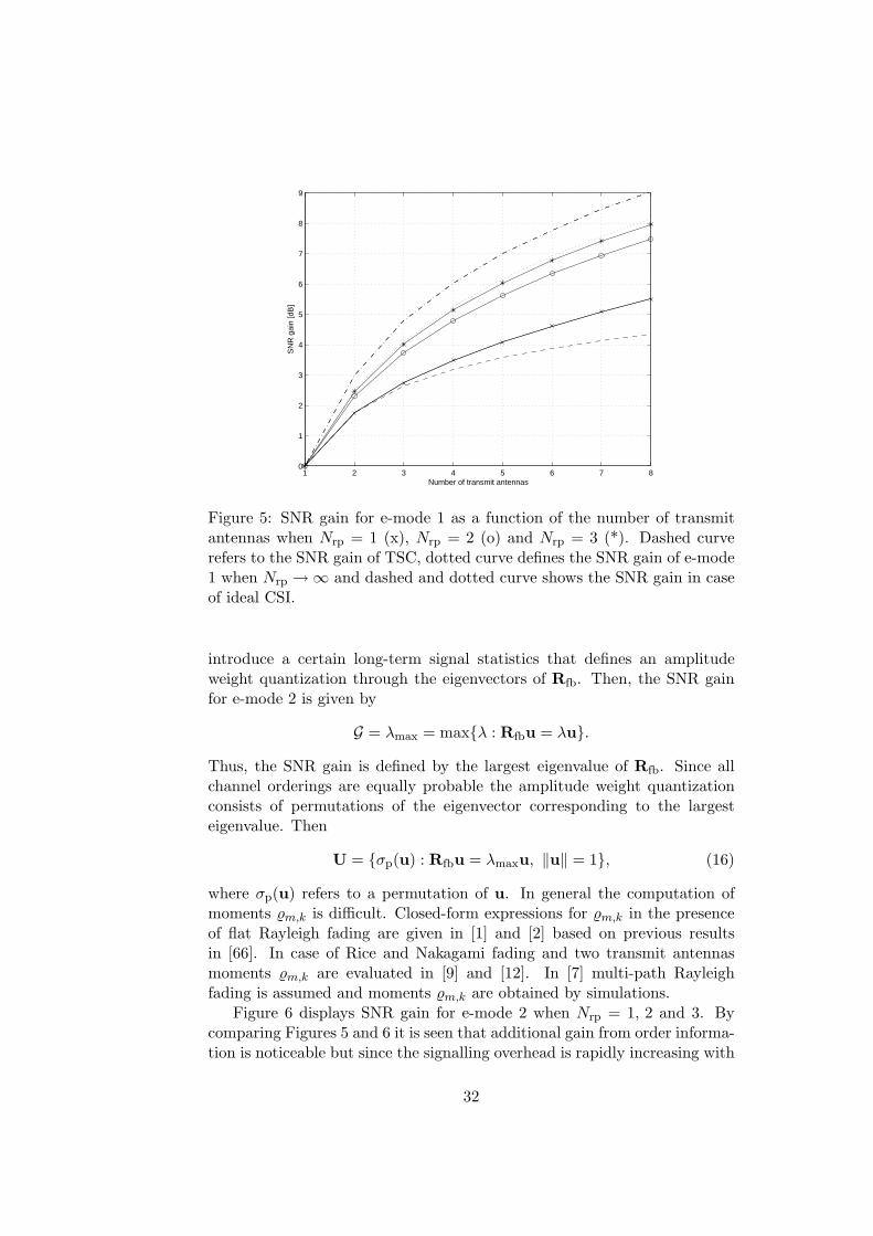
Figure 5: SNR gain for e-mode 1 as a function of the number of transmitantennas when Nrp = 1 (x), Nrp = 2 (o) and Nrp = 3 (*). Dashed curverefers to the SNR gain of TSC, dotted curve defines the SNR gain of e-mode1 when Nrp →∞ and dashed and dotted curve shows the SNR gain in caseof ideal CSI.

introduce a certain long-term signal statistics that defines an amplitudeweight quantization through the eigenvectors of Rfb. Then, the SNR gainfor e-mode 2 is given by

G = λmax = maxλ : Rfbu = λu.Thus, the SNR gain is defined by the largest eigenvalue of Rfb. Since allchannel orderings are equally probable the amplitude weight quantizationconsists of permutations of the eigenvector corresponding to the largesteigenvalue. Then

U = σp(u) : Rfbu = λmaxu, ‖u‖ = 1, (16)

where σp(u) refers to a permutation of u. In general the computation ofmoments %m,k is difficult. Closed-form expressions for %m,k in the presenceof flat Rayleigh fading are given in [1] and [2] based on previous resultsin [66]. In case of Rice and Nakagami fading and two transmit antennasmoments %m,k are evaluated in [9] and [12]. In [7] multi-path Rayleighfading is assumed and moments %m,k are obtained by simulations.

Figure 6 displays SNR gain for e-mode 2 when Nrp = 1, 2 and 3. Bycomparing Figures 5 and 6 it is seen that additional gain from order informa-tion is noticeable but since the signalling overhead is rapidly increasing with

32

1 2 3 4 5 6 7 80

1

2

3

4

5

6

7

8

9

Number of Antennas

SN

R g

ain

[dB

]

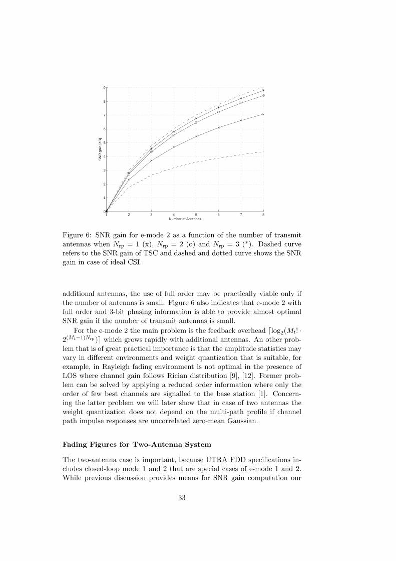
Figure 6: SNR gain for e-mode 2 as a function of the number of transmitantennas when Nrp = 1 (x), Nrp = 2 (o) and Nrp = 3 (*). Dashed curverefers to the SNR gain of TSC and dashed and dotted curve shows the SNRgain in case of ideal CSI.

additional antennas, the use of full order may be practically viable only ifthe number of antennas is small. Figure 6 also indicates that e-mode 2 withfull order and 3-bit phasing information is able to provide almost optimalSNR gain if the number of transmit antennas is small.

For the e-mode 2 the main problem is the feedback overhead dlog2(Mt! ·2(Mt−1)Nrp)e which grows rapidly with additional antennas. An other prob-lem that is of great practical importance is that the amplitude statistics mayvary in different environments and weight quantization that is suitable, forexample, in Rayleigh fading environment is not optimal in the presence ofLOS where channel gain follows Rician distribution [9], [12]. Former prob-lem can be solved by applying a reduced order information where only theorder of few best channels are signalled to the base station [1]. Concern-ing the latter problem we will later show that in case of two antennas theweight quantization does not depend on the multi-path profile if channelpath impulse responses are uncorrelated zero-mean Gaussian.

Fading Figures for Two-Antenna System

The two-antenna case is important, because UTRA FDD specifications in-cludes closed-loop mode 1 and 2 that are special cases of e-mode 1 and 2.While previous discussion provides means for SNR gain computation our

33

goal here is to illustrate the diversity benefit of e-mode 1 and 2 throughfading figure. This measure was first introduced in [67] and [68] and con-ventionally it is used as a fading parameter in Nakagami fading distributionthat gives one-sided Gaussian distribution if F = 1/2 and Rayleigh distribu-tion if F = 1. Values F < 1 correspond to deeper fading than the Rayleighwhile values F > 1 represent shallower fading than the Rayleigh.

As a reference we use the fading figure of TSC and, on the other hand, thefading figure in case of ideal feedback. We begin with TSC. The probabilitydensity function (PDF) of maximum taken over Mt exponentially distributedvariables is of the form

f(γ) = Mte−γ(1− e−γ)Mt−1 =

Mt∑

m=1

(Mt

m

)(−1)m+1m · e−mγ ,

where the latter equality is obtained by using the binomial expansion. Fur-thermore, after substituting t = mγ and applying the definition of Gammafunction ((6.1.1) of [69]) we find that

∫ ∞

0γne−mγdγ =

n!mn+1

. (17)

Hence,for TSC the moments of SNR are found to be

Eγn =Mt∑

m=1

(Mt

m

)(−1)m+1n!

mn, n ∈ N. (18)

If ideal CSI is available in the transmitter, SNR γ = ‖H‖2 follows the χ2

distribution with 2Mt degrees of freedom,

f(γ) =1

Γ(Mt)γMt−1e−γ , (19)

where Γ refers to the gamma-function. By (6.1.1) of [69] we find that themoments in case of ideal feedback are given by

Eγn = Γ(Mt + n)/Γ(Mt). (20)

The fading figure for TSC can be computed by using (18) and for systemwith ideal feedback we can use (20). In the latter case it is easily seen thatF = Mt. Hence, in the presence of flat Rayleigh fading and partial feedback,the value of fading figure for any closed-loop algorithm is upper bounded bythe number of transmit antennas.

Let us next consider the fading figure for e-mode 1 and 2 in case of twotransmit antennas. The second moment of SNR for e-mode 1 and 2 can becomputed from

Ez2 = E(u21γ(1) + u2

2γ(2) + 2u1u2√

γ(1)γ(2) cosφ)2. (21)

34

By expanding this formula we find that the required second moment isobtained provided that expectations

Ecoskφ, k ∈ 1, 2, Eγ2−δ(1) γδ

(2), δ ∈ 0, 1/2, 1, 3/2, 2 (22)

can be computed. The former expectation for k = 1 is known from (11) andafter a similar computation we find that

Ecos2φ = 1/2 · (1 + cNrp−1). (23)

It remains to compute the latter expectation in (22). We first note that thejoint distribution of γ(1) and γ(2) is given by

f(γ(1), γ(2)) = 2 ·

e−|γ|, γ1 ≥ γ2,

0, otherwise,(24)

where we have denoted γ = (γ1, γ2) and |γ| = γ1 + γ2. Second expectationin (22) is not difficult to compute directly but instead we apply substitution,γ2 = tγ1, change the order of the integration and then substitute s = γ1(1+t). Then we find that

Eγ2−δ(1) γδ

(2) =∫ ∞

0s3e−sds ·

∫ 1

0

2tδdt

(1 + t)4= 6 ·

∫ 1

0

2tδdt

(1 + t)4=: 6 · Iδ. (25)

We use this computation method because its idea is found useful later inthe analysis of link capacity. The integral Iδ can be computed by usingelementary means. Resulting formulas are

I0 =712

, I 12

=112

+π

16, I1 =

16, I 3

2= − 1

12+

π

16, I2 =

112

. (26)

Based on (21), (11), (23), (25) and (26) we can compute the second momentof SNR in case of e-mode 1 and 2. Then, using the SNR gains that werecomputed in the previous section we obtain fading figures. Table 1 gives thefading figures for TSC, and e-mode 1 and 2. The results show that e-mode 1and 2 provide clearly better fading figures than TSC but differences are smallindicating that all studied methods provide good diversity gain. Since thefading figure for the Alamouti code [45] and for ideal CSI in the transmitteris 2, we note that closed-loop methods with partial side information arenot able to provide full diversity benefit if it is measured in terms of fadingfigure.

SNR Gain in Multi-path Fading

Here we adopt a multi-path Rayleigh fading model and assume Rake com-bining over signal paths. Now H is a matrix with columns hm that consistsof the channel impulse responses hm,l corresponding to L channel paths.

35

TSC e-mode 1, (2) e-mode 1, (3) e-mode 2, (2) e-mode 2, (3)1.8000 1.9104 1.9123 1.9867 1.9913

Table 1: Fading figures for TSC and two-antenna e-mode 1 and 2. Thenumber of phase bits is given in brackets.

In multi-path Rayleigh fading model coefficients hm,l are independent zero-mean Gaussian random variables. Furthermore, we denote E|hm,l|2 = 2σ2

l ,l = 1, 2, . . . , L and use scaling

E‖hm‖2 = 2L∑

l=1

σ2l = 1.

Consider the feedback quantization in a detailed manner. In two antennacase transmit weights are of the form w1 = u1, w2 = u2e

jφ, where 0 ≤u1, u2 ≤ 1 and uniform quantization of the phase φ is clearly a good choiceif transmit antennas are uncorrelated. In the following we show that optimalamplitude weights are of the form

u1,2 =1

2

(1±

(1 +

π2c2Nrp

4

)−1/2)1/2, (27)

where the ’+’ sign corresponds to the weight u1 of the stronger channel whilethe ’-’ sign corresponds to the weight u2 of the weaker channel. For flatfading this result is known already from [1]. However, it is not immediatelyclear that weights (27) represent the best choice also in the presence of multi-path Rayleigh fading. In fact, from [9] and [12] it is known that weights (27)are not optimal in Rice and Nakagami fading channels. This question onoptimal weights is of interest because UTRA FDD standards specify fixedamplitude weights while applied 3GPP test channels use various profiles [70].At this stage we note that specified amplitude weights in UTRA FDD aregiven by u1, u2 ∈ √0.8,

√0.2 while numeric values of optimal weights

according to (27) are√

0.7735 and√

0.2265. In flat Rayleigh fading channelthe difference in obtained SNR gains when applying these different weightsis of no practical meaning - it os less than 0.005 dB - but the squares of thespecified weights admit a simple digital expression.

Let us consider the equation

‖u1h(1)+u2ejφh(2)‖2−‖u2h(1)+u1e

jφh(2)‖2 = (u21−u2

2)(‖h(1)‖2−‖h(2)‖2

).

From this equation we find that independently from φ, the better SNRis always achieved if more power is allocated into the transmit antenna

36

providing larger received power. Based on this observation we assume thatu1 > u2 in the following discussion. Further, we obtain

‖Hw‖2 = u21‖h(1)‖2 + u2

2‖h(2)‖2 + 2u1u2|hH(1)h(2)| cosψ, (28)

where ψ = φ + θ and θ = arg(hH(1)h(2)) is uniformly distributed on (−π, π).

We note that ψ and |hH(1)h(2)| are independent. Moreover, the order of

channel vectors has no effect to the absolute value of the inner product be-tween h(1) and h(2). After the adjustments the relative phase ψ is uniformlydistributed on (−π/2Nrp , π/2Nrp). Then we have

Ez = uTRfbu, Rfb =

(E‖h(1)‖2 cNrpE|hH

(1)h(2)|cNrpE|hH

(1)h(2)| E‖h(2)‖2

). (29)

After these preparations we are ready to prove that (27) defines optimalweights also in case of multi-path Rayleigh fading when the paths are un-correlated. Note this is also true for ideal CSI feedback and for Grassmaniancodebooks [63, 64] as observed in [64].

Let u1 and u2 be the components of the eigenvector of the largest eigen-value of Rfb, defined in (29). After solving the corresponding eigenvalueproblem it is found that

u1,2 =1

2

(1±

(1 + ρ2

)−1/2)1/2(30)

where ρ is given by

ρ =2cNrpE|hH

(1)h(2)|E‖h(1)‖2 − E‖h(2)‖2 . (31)

Hence, by (27) it remains to show that ρ = πcNrp/2. Since h(1) and h(2)

consists of uncorrelated Gaussian zero-mean variables the following trick canbe used: Assume e-mode 1 with Nrp = 1 and define

h1 =1√2

(h1 + h2

), h2 =

1√2

(h1 − h2

). (32)

Then it is evident that the SNR gain of e-mode 1 with Nrp = 1 can beobtained from the formula

G = E‖h(1)‖2. (33)

Furthermore, it is not difficult to see that the elements of the vectors h1 andh2 are distributed identically with the elements of vectors h1 and h2. Thus,

E‖h(1)‖2 = E‖h(1)‖2. (34)

37

On the other hand, when computing the SNR gain of 1-bit phasing from (28)it is found that

G =12(E‖h(1)‖2+ E‖h(2)‖2) + c1E|hH

(1)h(2)|. (35)

By combining (33), (34), (35) and equality c1 = 2/π we find that

E‖h(1)‖2 =12(E‖h(1)‖2+ E‖h(2)‖2) +

2π· E|hH

(1)h(2)|. (36)

From (31) and (36) it is seen that ρ = πcNrp/2 in (30) and thus, the shapeof the delay profile does not effect the value of the optimal weights as far aschannel paths are uncorrelated and Rayleigh fading is assumed.

Let us next consider the SNR gain for two-antenna e-mode 1 and 2 inthe presence of multi-path fading. For e-mode 1 it is seen from (28) that

G = 1 + cNrpE|hH(1)h(2)|. (37)

Before giving the expectation in (37) we deduce a similar expression for theSNR gain of mode 2. By computing the largest eigenvalue of Rfb, definedin (29), we obtain

G = 1 +(1− E‖h(1)‖2E‖h(2)‖2+ c2

NrpE|hH

(1)h(2)|2) 1

2. (38)

Keeping in mind the scaling

E‖H‖2 = E‖h(1)‖2+ E‖h(2)‖2 = 2 (39)

we find from (36) that

E‖h(1)‖2 = 1 +2π

E|hH(1)h(2)|, E‖h(2)‖2 = 1− 2

πE|hH

(1)h(2)|. (40)

After combining (38) and (40) we finally obtain the following form for theSNR gain of e-mode 2,

G = 1 +( 4

π2+ c2

Nrp

) 12 E|hH

(1)h(2)|. (41)

Thus, for final SNR gain formulas of e-mode 1 and 2 it remains to computeE|hH

(1)h(2)|. This has been done in [3] where it was shown that

E|hH(1)h(2)| =

π

2

L∑

l=1

σ2l

L∏

k=1,k 6=l

σ4l

σ4l − σ4

k

. (42)

This formula is valid provided that mean path powers are distinct. In thepresence of multiple receive antennas and single path channel we can useLemma 2 of [3],

E|hH(1)h(2)| =

√π · Γ(Mr + 1/2).

38

Channel profile Rayleigh Ped. A Ped. B Veh. Ae-mode 1, Nrp = 1 1.7609 dB 1.7446 dB 1.3012 dB 1.3839 dBe-mode 1, Nrp = 2 2.3226 dB 2.3024 dB 1.7436 dB 1.8489 dBe-mode 1, Nrp = 3 2.4683 dB 2.4472 dB 1.8603 dB 1.9712 dBe-mode 2, Nrp = 1 2.3226 dB 2.3024 dB 1.7436 dB 1.8489 dBe-mode 2, Nrp = 2 2.7092 dB 2.6865 dB 2.0549 dB 2.1748 dBe-mode 2, Nrp = 3 2.8199 dB 2.7966 dB 2.1450 dB 2.2690 dB

Table 2: SNR gains for two-antenna e-mode 1 and 2 assuming differentchannel profiles of [70].

The formula in general case, where the number Mr of receive antennas islarger than one and multi-path channel is assumed, can be deduced similarlywith (42).

Table 2 depicts the obtained SNR gains for e-mode 1 and 2 when Mr = 1and different channel profiles are assumed. Results show that SNR gainsof e-mode 1 and 2 are noticeably corrupted due to the multi-path fading.Finally, we note that the SNR gain in the presence of multi-path Rayleighfading is also studied in [7] where the case Mt > 2 is considered.

3.3 Computation of Link Capacity

Here we consider the link capacity for e-mode 1 and 2. First we focus oncapacity (6) that assumes constant transmit power and optimal rate adap-tation to the channel fading. As mentioned, capacity (6) is an appropriateperformance measure in HSDPA where power control is not applied on theshared channel.

It will turn out, however, that the computation of exact closed-formexpression for (6) is extremely difficult in case of closed-loop transmit diver-sity methods. Contrary to exact expression a simple upper bound can beobtained through the estimate

Cora(γ) ≤ B · log2

(1 + γ · Ez) = B · log2

(1 + γ · G)

(43)

that applies the fact that logarithm is a concave function. Hence the ca-pacity of a closed-loop transmit diversity method is upper bounded by thecapacity of AWGN channel where mean SNR is scaled by the SNR gainG. Since (43) provides only a loose bound it is of interest to find a bet-ter estimate for capacity (6). In this section we introduce such a simpleand accurate approximation and also provide an error analysis for the givenapproximation in case of two transmit antennas.

We recall that by (3) the instantaneous received SNR for a closed-loop

39

transmit diversity method can be expressed in the form

z(γ, φ) =∣∣∣

Mt∑

m=1

um√

γm · ejφm

∣∣∣2, γm = |hm|2, (44)

where φ1 = 0 and adjusted phases φm, m = 2, 3, . . . ,Mt are uniformly dis-tributed on the interval (−π/2Nrp , π/2Nrp). In general the distribution of zis difficult to deduce but (44) indicates that SNR gain can be computed pro-vided that distributions of γ and φ are known. Since channel coefficients areuncorrelated and phase and amplitude adjustments are done independentlywe find that

f(γ, φ) = f(γ)f(φ) = f(γ)Mt∏

m=2

fm(φm), |γ| =Mt∑

m=1

γm, (45)

where fm refer to the uniform distribution function corresponding to φm,resulting from the Nrp-bit phase adjustments. The distribution of γ de-pends on the amplitude information. In case of e-mode 1 there is no suchinformation and f(γ) = e−|γ|.

Computation of capacity (6) can be based on the conditional distribu-tion. Then

Cora(γ) = B

∫log2(1 + γ · z(γ, φ))f(γ, φ)dγdφ, (46)

where dγ = dγ1dγ2 . . . dγMt and dφ = dφ2 . . . dφMt . We introduce an ap-proximation by which the computation of (46) can be greatly simplified. Byusing the basic properties of the logarithm we find that

log2(1 + γ · z(γ, φ)) = log2(1 + γ · G|γ|/Mt) + log2(1 + ρ(γ, φ)), (47)

where ρ is given by

ρ(γ, φ) = γ · z(γ, φ)− G|γ|/Mt

1 + γ · G|γ|/Mt. (48)

According to the decomposition (47) we can write

Cora(γ) = Cora(γ) + ε(γ), (49)

where ε represents the error of the approximation

Cora(γ) = B

∫log2(1 + γ · G|γ|/Mt)f(γ, φ)dγdφ

= B

∫log2

(1 + γ · G|γ|/Mt

)f(γ)dγ ≈ Cora(γ).

(50)

40

Let us briefly explain the idea leading to this approximation. Since G = Ezand E|γ|/Mt = 1 we find that the expectation in the numerator of (48)vanishes. Then it can be expected that the error

ε(γ) = B · Elog2(1 + ρ)

is small. Furthermore, we note that if G = 1 then Cora represents thelink capacity in the presence of orthogonal design such as rate 1 space-timeblock code. Such a system provides full diversity benefit but no coherentcombining gain. In (50) this additional gain from coherent combining isembedded into the SNR gain G. On the other hand, if perfect CSI is availablein the transmitter, then G = Mt and Cora gives the exact capacity of Mt

antenna receiver maximal ratio combining. The closed-form expression forthe capacity of receiver maximal ratio combining is deduced in [54],

Cora,MRC(γ)=B log2(e)(PMt

(−1

γ

)E1

(1γ

)+

Mt−1∑

k=1

1kPk

(1γ

)PMt−k

(−1

γ

)), (51)

where PMt is the Poisson distribution function, defined by

PMt(x) = e−x ·Mt−1∑

m=0

xm

m!. (52)

From (50) and (51) we find that our approximation reads as

Cora = Cora,MRC

( GMt

· γ). (53)

Hence, the applied approximation reduces the computation of the link ca-pacity to the computation of SNR gain that is a much more straightforwardoperation. Figure 7 depicts the link capacity (6) as a function of mean SNRfor two-antenna e-mode 1 (Nrp = 2) and e-mode 2 (Nrp = 3) correspondingto UTRA FDD mode 1 and 2 respectively. The results show that e-mode1 and 2 provide better capacity than TSC while the performance differencebetween e-mode 1 and 2 is small. The performance difference between e-mode 2 and ideal case is very small as well. For single antenna system,TSC, and ideal case the exact closed-form expressions are applied and fore-mode 1 and 2 the approximation (53) is employed. Point values (x) and(o) corresponding to e-mode 1 and 2 were simulated by using 106 samples.As found from Figure 7 there is no visible error between simulated pointvalues and approximation curves.

Although simulations hint that error ε in (49) is small, it is worth ofstudying the error more carefully. In general, an appropriate error analysisshould contain the following stages:

• Confirm that the given approximation is well defined.

41

• Find an upper bound for the approximation error.

Clearly, approximation (49) is well defined if ρ > −1. Let us show thatthis condition is valid provided that G > 1 and Nrp > 1. For that purpose weexpand (44). In the resulting formula cross-terms containing cos(φm − φk),m 6= k, are non-negative because |φm − φk| ≤ π/2. We note that in two-antenna case cross-term is non-negative also in case Nrp = 1. We attain alower bound

z(γ, φ) ≥Mt∑

m=1

u2mγm ≥ |γ|/Mt, (54)

where the second inequality is trivially true for e-mode 1 and in case ofe-mode 2 it reflects the fact that it is always a better strategy to put morepower on the stronger channel than to share transmit power evenly betweenchannels. By applying (54) to (48) we find that

ρ(γ, φ) ≥ − γ · G|γ|/Mt

1 + γ · G|γ|/Mt

(G − 1G

)≥ −G − 1

G . (55)

Hence, if G > 1 then ρ > −1. Condition G > 1 is not restrictive because itis valid always when closed-loop method gives SNR gain.

It remains to find an upper bound for the approximation error. In theforthcoming error analysis we apply the formula

log2(1 + ρ) = log2(e)(ρ− ρ2

2(1 + ζ)2), min0, ρ ≤ ζ ≤ max0, ρ, (56)

that is obtained by using Taylor’s expansion with respect to ρ. To avoidintolerable complexity we assume from this on that Mt = 2. Next we showthat the expectation of ρ vanishes. We begin this proof by writing

ρ(γ, φ) = z(ξ, φ)− G|ξ|/2, ξm =γm

1/γ + G|γ|/2.

By taking the expectation with respect to γ and φ we obtain

Ez(ξ, φ) = u21Eξ(1)+ u2

2Eξ(2)+ 2u1u2E√

ξ(1)ξ(2)cNrp . (57)

The required expectations are computed similarly with (25). First wesubstitute γ2 = tγ1. Then

Eξ1−δ(1) ξδ

(2) =∫ ∞

0

∫ 1

0

2γ21tδe−γ1(1+t)

1/γ + Gγ1(1 + t)/2dt dγ1. (58)

In the second stage we change the integration order and substitute s =γ1(1 + t). The resulting formula reads as

Eξ1−δ(1) ξδ

(2) =∫ 1

0

2tδdt

(1 + t)3∫ ∞

0

s2e−s

1/γ + Gs/2ds

= Iδ · Iξ. (59)

42

−5 0 5 10 15 200

1

2

3

4

5

6

7

8

SNR [dB]

Cap

acity

[bits

/s/H

z]

Figure 7: Link capacity for two-antenna e-mode 1 when Nrp = 2 (x) ande-mode 2 when Nrp = 3 (o) in the presence of Rayleigh fading, constanttransmit power and optimal rate adaptation. Dotted curve refers to thecapacity of single antenna transmission, dashed curve indicates the capacitygiven by TSC and dashed and dotted curve refers to the capacity in case ofideal CSI.

For (57) we need I0, I1/2 and I1. The computation of these integrals isa straightforward task and results in

I0 = 3/4, I1/2 = π/8, I1 = 1/4. (60)

Hence, we have

Ez(ξ, φ) =(3

4u2

1 +14u2

2 +πcNrp

4u1u2

)Iξ =

G2· Iξ. (61)

On the other hand, using the same substitutions as in (58) and (59) weobtain

EG

2|ξ|

=G2

(Eξ(1)+ Eξ(2)

)=G2· Iξ.

By combining the last two equations we find that Eρ = 0.Now we know that the distribution of ρ is concentrated on 0 in which

point the error ε vanishes. For the final error bound we need the secondmoment of ρ. This is due to the estimate

|ε| = B log2(e)∣∣∣E

ρ2

2(1 + ζ)2∣∣∣ ≤ B log2(e)max

12(1 + ζ)2

Eρ2, (62)

43

that is obtained from (56). By (55) it is found that

1 + ζ ≥ 1 + min0, ρ ≥ 1− G − 1G =

1G . (63)

Then (62) implies

|ε| ≤ B log2(e) ·12· G2 · Eρ2 =: ε (64)

and it remains to deduce the second moment of ρ.It is not difficult to see that Eρ2 attains a closed-form expression.

Since the resulting formula is relatively complex we only compute a boundfor the asymptotic error ε∞ that is defined by

ε∞ = B · Elog2(1 + ρ∞), ρ∞ = limγ→∞ ρ.

We begin by expanding ρ2∞ as follows

Eρ2∞ = Ez(ξ, φ)2 − 2Ez(ξ, φ)+ 1. (65)

Hence, we need to compute the first and the second moment of z(ξ, φ) withrespect to γ and φ. For the first moment there holds by (61)

limγ→∞Ez(ξ, φ) =

G2

limγ→∞ Iξ =

∫ ∞

0se−sds = 1. (66)

In a similar manner as in (21) and (22) the evaluation of the second momentof z(ξ, φ) is reduced to the computation of moments

Eξ2−δ(1) ξδ

(2), δ ∈

0, 1/2, 1, 3/2, 2

.

Furthermore, by using the method of (58) and (59) we find that

limγ→∞Eξ2−δ

(1) ξδ(2) = Iδ, (67)

where values of Iδ are available from (26). Thus, by combining (64) and (65)-(67) we can compute an upper bound ε∞ for the error ε∞. The resultingerror bounds for our capacity approximations are given in Table 3 showingthat asymptotic approximation errors are small.

Fast power control approximately inverts the dedicated channels inUTRA FDD, and a suitable form of capacity is given by (7), where E1/zrepresents the power that is required to compensate the fading. In the com-putation of E1/z we apply the approximation

E1

z

=

Mt

G E 1|γ|

− ε ≈ Mt

G E 1|γ|

, (68)

44

ε∞ [bps/Hz] Nrp = 1 Nrp = 2 Nrp = 3e-mode 1 0.0601 0.0329 0.0344e-mode 2 0.0329 0.0056 0.0039

Table 3: Upper bounds for capacity approximation error in case of twotransmit antennas.

where ε is the corresponding error. Since |γ| follows the χ2-distribution with2Mt degrees of freedom it is easily found that [54]

E1/|γ| = 1/(Mt − 1). (69)

The approximation Cinv of Cinv is then given by

Cinv = B · log2

(1 +

(Mt − 1)GMt

· γ). (70)

When G = 1 Equation (70) provides the capacity of a rate 1 space-timeblock code that applies orthogonal design.

As an additional reference we consider the capacity of TSC. From [54] itis known that for TSC

E 1

γ(1)

= lim

ω→0+Mt

Mt−1∑

k=0

(−1)k

(Mt − 1

k

)E1((1 + k)ω), (71)

where E1 is the first order exponential integral function defined by

En(x) =∫ ∞

1

e−xt

tndt, arg(x) < π, n ∈ N0. (72)

The computation of the rather complex-looking limit (71) is not carried outin [54], and therefore we will do it here. Let γ be arbitrary but fixed positivenumber. Then, if ω is small we have by (5.1.11) of [69]

E1((1 + k)ω) = −e0 − log((1 + k)ω) = −e0 − log ω − log(1 + k),

where e0 is Euler’s constant. Moreover, by Binomial Theorem there holds

0 = (1− 1)Mt−1 =Mt−1∑

k=0

(−1)k

(Mt − 1

k

).

Hence we find that the term containing ω vanishes in (71) and

E 1

γ(1)

= Mt

Mt−1∑

k=0

(−1)k+1

(Mt − 1

k

)log(1 + k)

=Mt∑

k=1

(Mt

k

)k · log(k).

45

−5 0 5 10 15 200

1

2

3

4

5

6

7

SNR [dB]

Cap

acity

[bits

/s/H

z]

Figure 8: Link capacity for e-mode 1 when Nrp = 2 (x) and for e-mode 2when Nrp = 3 (o) in the presence of Rayleigh fading, ideal PC, and fixed-rate modulation and coding. Dashed curve refers to the capacity given byTSC and dashed and dotted curve refers to the capacity in case of ideal CSI.

Figure 8 shows Cinv for two-antenna e-mode 1 (Nrp = 2) and e-mode2 (Nrp = 3). The corresponding discrete values (x) and (o) were simu-lated by using 106 samples. The results show that UTRA FDD closed-loopmodes provide better capacity than TSC also in case of PC and fixed-ratemodulation and coding. Again the gap between e-mode 2 and ideal case issmall.

According to Figure 8 the approximation error is again very small. Inthe following we show this also analytically. We deduce the error bound forthe approximation (70) in case of two antennas. There holds

ε(γ) = Cinv(γ)− Cinv(γ) = B · log2

( 1 + γ/E1/z1 + G(Mt − 1)γ/Mt

). (73)

Let us substitute the approximation (68) in (73) and use (69). Then we findthat

ε(γ) = B · log2

(1 + γ/(Mt/G(Mt − 1)− ε

)

1 + G(Mt − 1)γ/Mt

). (74)

Again we concentrate on the asymptotic SNR region. Then by (74) thereholds

ε∞ = B · log2

( 11− ε · G(Mt − 1)/Mt

). (75)

46

Furthermore, since ε is small, we get

ε∞ ≈ B · log2(e) ·G(Mt − 1)

Mt· ε

and it remains to find the error ε. To this end we can apply the identity

1z(γ, φ)

=Mt

G|γ| ·1

1 + ρ∞(γ, φ), ρ∞(γ, φ) =

z(γ, φ)− G|γ|/Mt

G|γ|/Mt

and Taylor’s expansion

11 + ρ∞

= 1− ρ∞ +ρ2∞

(1 + ζ)3, min0, ρ∞ ≤ ζ ≤ max0, ρ∞.

After combining (68) and the last two equations we find that

ε =Mt

G(E

ρ∞(γ, φ)|γ|

− E

ρ∞(γ, φ)2

(1 + ζ)3|γ|)

. (76)

Here the first expectation on the right-hand side vanishes. To show this,we need to compute expectations Eξ1−δ

(1) ξδ(2), δ ∈ 0, 1/2, 1, where ξm =

Mtγm/G|γ|2. By using the same substitutions as in previous cases we obtain

Eξ1−δ(1) ξδ

(2) =2G

∫ 1

0

2tδdt

(1 + t)3=

2G · Iδ.

The values of Iδ were given in (60). Hence, similarly with (57) and (61) wefind that

Ez(γ, φ)

/|γ|2 = G/2. (77)

Then, after applying the definition of ρ∞ and equality E1/|γ| = 1 by (69)we see that the first expectation on the right-hand side of (76) vanishes.Now, by (76) and the estimate (63) we find that

|ε| ≤ Mt · G2 · Eρ∞(γ, φ)2

/|γ| =: ε.

In the computation of bound ε we need the expression

ρ∞(γ, φ)2/|γ| = ((2/G)2z(γ, φ)2/|γ|3 − 4z(γ, φ)/G|γ|2 + 1/|γ|).

Using this equality, the result (77) and equality E1/|γ| = 1 we obtain

ε = G2 · ((2/G)2Ez(γ, φ)2/|γ|3 − 1).

After suitable substitutions it is seen that the expectation on the right canbe expressed in terms of Iδ for which numeric values were given in (26). Nowwe are able to compute the values of ε.

Table 4 gives analytical upper bounds for the error of the approxima-tion (70) in two-antenna case.

47

ε[bps/Hz] Nrp = 1 Nrp = 2 Nrp = 3e-mode 1 0.0902 0.0561 0.0607e-mode 2 0.0561 0.0104 0.0074

Table 4: Analytic upper bounds for approximation error ε in case of twotransmit antennas.

3.4 Computation of BEP

In the conventional approach the bit error probability Pe for a certain SNRis computed by using the formula

Pe(γ) = EPmod(γ · z) =∫

Pmod

(γ · z(γ, φ)

)f(γ, φ)dγdφ, (78)

where Pmod is the error rate of the modulation. We consider e-mode 1in general case while e-mode 2 is discussed only in case Mt = 2. In thepresentation we follow [5].

For single antenna transmission as well as for MRC and TSC closed-formexpressions of (78) are known for various modulation techniques. On thecontrary, BEP formulas for advanced closed-loop transmit diversity methodssuch as e-mode 1 and e-mode 2 — that apply partial CSI — are widelyunknown. Recently, lower bounds for symbol error probabilities of closed-loop feedback schemes were formulated in [75]. These bounds are tight forgood codebooks derived according to design principles in [63, 64]. Here weconcentrate on e-mode 1 and 2 and show a method to compute BEP inasymptotic SNR region. Furthermore, we recall an approximation whichadmits an accurate BEP estimate for e-mode 1 and 2 in the whole SNRscale. For simplicity we assume BPSK modulation.

We begin with e-mode 1 and write

Pe(γ) =∫

Ωφ

f(φ)(∫

RMt+

Pmod

(γ · z(γ, φ)

)e−|γ|dγ

)dφ, (79)

where f(φ) is the PDF of adjusted relative phases and Ωφ is given by

Ωφ = φ ∈ RMt−1 : −π/2Nrp ≤ φm ≤ π/2Nrp , m = 1, 2, . . . , Mt − 1.We first modify the formula (79) through the substitution γ = sr,

s > 0, r = (r1, . . . , rMt−1, 1), dγ = sMt−1dr1 . . . drMt−1ds = sMt−1drds.

The resulting expression reads as

Pe(γ) =∫

Ωφ

f(φ)(∫

R+

(∫

RMt−1+

Pmod

(γ · s · z(r, φ)

)sMt−1e−s|r|dr

)ds

)dφ.

48

To find a suitable expression for asymptotic BEP we change the integrationorder and set t = γ · s · z(r, φ). Then

Pe(γ) =(1

γ

)Mt∫

Ωφ

∫

RMt−1+

f(φ)z(r, φ)Mt

(∫

R+

Pmod(t)tMt−1e− t|r|

γ·z(r,φ) dt)drdφ.

Let us compute the integral in the brackets when SNR grows without limit.For that purpose we use the equation

∫

R+

Pmod(t)tMt−1e−atdt =(− d

da

)Mt−1∫

R+

Pmod(t)e−atdt, (80)

that is valid provided that integral on the right is finite. Since BPSK mod-ulation is employed we have by (7.4.19) of [69]

∫

R+

Pmod(t)e−atdt =12

∫

R+

erfc(√

t)e−atdt =12a

(1−

√1

1 + a

).

After applying Taylor’s expansion to (1 + a)−1/2 we further obtain∫

R+

Pmod(t)e−atdt =∞∑

k=0

dkak, dk =

(−1)k(2k + 1)!22k+2k!(k + 1)!

.

Now it is a simple task to compute the limit in (80). We have

limγ→∞

∫

R+

Pmod(t)tMt−1e−atdt = limγ→∞

(− d

da

)Mt−1∞∑

k=0

dkak

= (−1)Mt−1(Mt − 1)! · dMt−1 =(2Mt − 1)!22MtMt!

.

(81)

By using the equation (81) we attain an asymptotic formula

Pe(γ) =(1

γ

)Mt (2Mt − 1)!22MtMt!

∫

Ωφ

∫

RMt−1+

f(φ)drdφ

z(r, φ)Mt

that is valid when γ >> 1 and BPSK modulation is assumed. For compari-son purposes we write

Pe(γ) =(

2Mt − 1Mt

)( AMt,Nrp

4(γ/Mt)

)Mt

, γ >> 1, (82)

where γ/Mt is the SNR per transmit antenna and AMt,Nrp is defined by

AMtr,Nrp =(Mt − 1)!

MMtt

∫

Ωφ

∫

RMt−1+

f(φ)drdφ

z(r, φ)Mt

1Mt . (83)

Formula (82) is handy because it is similar to the well-known asymptoticBEP formula of Mt-antenna MRC [71]. By setting AMt,Nrp = Mt in (82) we

49

Nrp 1 2 3 ∞A2,Nrp [dB] 1.505 2.198 2.340 2.386B2,Nrp [dB] 2.198 2.694 2.810 2.847

Table 5: Asymptotic BEP gains of e-mode 1 and 2 against rate=1 space-timeorthogonal design when Mt = 2.

obtain the BEP of receiver MRC while with AMt,Nrp = 1 Equation (82) pro-vides the BEP for rate 1 space-time orthogonal design. Hence, the constantAMt,Nrp in (82) indicates the coherent combining gain due to closed-loopadjustments.

In [5] it was shown — by a straightforward integration — that for two-antenna e-mode 1 there holds

A2,Nrp =1− 2Nrp−1

π sin π2Nrp−1

2 sin2 π2Nrp

12.

Following the reasoning of [5] we find that formula (82) is valid also fortwo-antenna e-mode 2 provided that AMt,Nrp is replaced with

B2,Nrp =2Nrp

π

∫ 1

0

∫ π/2Nrp

0

dφdr

(u21 + u2

2r + 2u1u2√

r cosφ)2

12.

Closed-form expression for B2,Nrp exists but it is omitted because it is rathercomplex. Table 5 gives values of A2,Nrp and B2,Nrp when Nrp = 1, 2, 3,∞. Werecall that in two-antenna case e-mode 1 with Nrp = 1 coincides with TSC.According to the results in Table 5 the UTRA FDD mode 1 and 2 provide0.693 dB and 1.305 dB gain against TSC in asymptotic BEP respectively.

In [5] it was also shown that for e-mode 1 with Mt antennas there holds

AMt,∞ =2Mt−1(Mt − 1)!

(2Mt − 1)!

1Mt .

Since e-mode 1 with ideal phasing is equivalent with receiver equal gaincombining, the computation of AMt,∞ provides also means to deduce theBEP of equal gain combining. If Mt > 2 and Nrp is finite, the computationof AMt,Nrp and BMt,Nrp is an open problem.

While (82) is valid when γ is large, it is of great importance to find also aBEP formula that is valid through the whole SNR range. This task is solvedin [5] showing that a good approximation in two-antenna case is given by

Pe(γ) =14

(1−

√γ/2

C2,Nrp + γ/2

)2(2 +

√γ/2

C2,Nrp + γ/2

), (84)

50

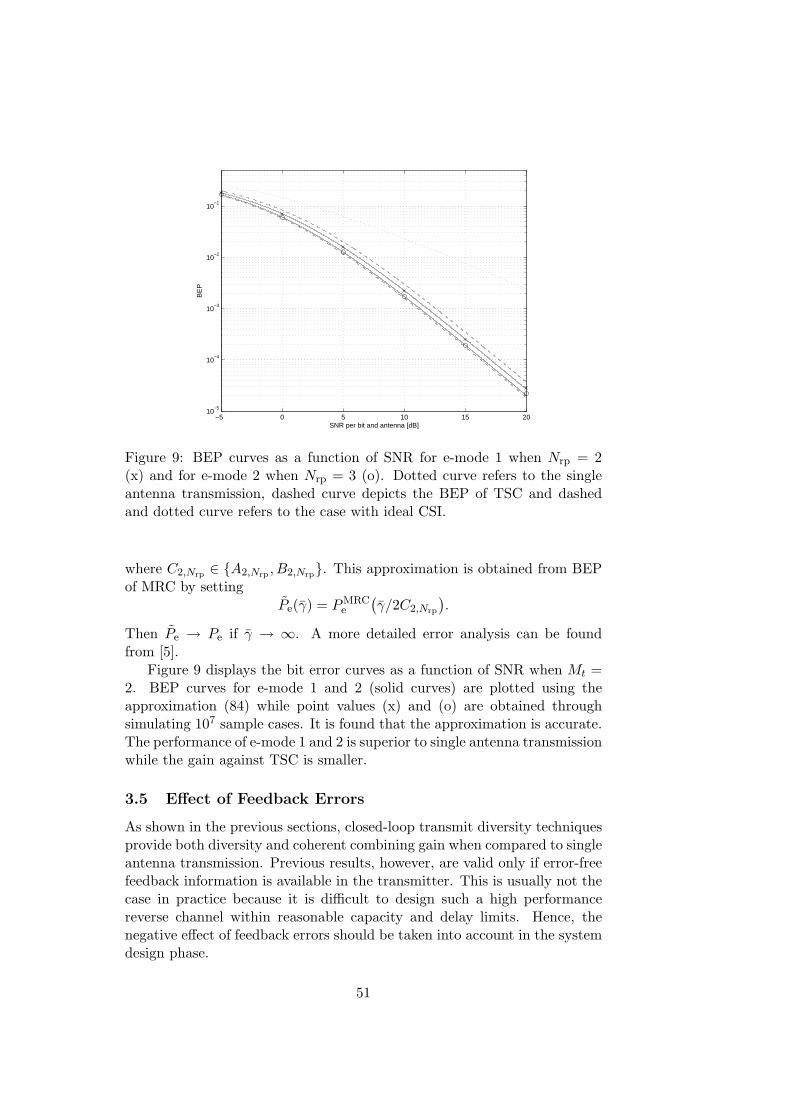
−5 0 5 10 15 2010

−5

10−4

10−3

10−2

10−1

BE

P

SNR per bit and antenna [dB]

Figure 9: BEP curves as a function of SNR for e-mode 1 when Nrp = 2(x) and for e-mode 2 when Nrp = 3 (o). Dotted curve refers to the singleantenna transmission, dashed curve depicts the BEP of TSC and dashedand dotted curve refers to the case with ideal CSI.

where C2,Nrp ∈ A2,Nrp , B2,Nrp. This approximation is obtained from BEPof MRC by setting

Pe(γ) = PMRCe

(γ/2C2,Nrp

).

Then Pe → Pe if γ → ∞. A more detailed error analysis can be foundfrom [5].

Figure 9 displays the bit error curves as a function of SNR when Mt =2. BEP curves for e-mode 1 and 2 (solid curves) are plotted using theapproximation (84) while point values (x) and (o) are obtained throughsimulating 107 sample cases. It is found that the approximation is accurate.The performance of e-mode 1 and 2 is superior to single antenna transmissionwhile the gain against TSC is smaller.

3.5 Effect of Feedback Errors

As shown in the previous sections, closed-loop transmit diversity techniquesprovide both diversity and coherent combining gain when compared to singleantenna transmission. Previous results, however, are valid only if error-freefeedback information is available in the transmitter. This is usually not thecase in practice because it is difficult to design such a high performancereverse channel within reasonable capacity and delay limits. Hence, thenegative effect of feedback errors should be taken into account in the systemdesign phase.

51

We show here that in the presence of feedback errors the asymptoticdiversity of the feedback schemes is equal to one which is similar to a singleantenna transmission. The same observation has been made in [57] assum-ing Gaussian distributed quantization error. This may seem to be a severedrawback of feedback schemes, but with proper feedback requirements sys-tem can be designed in such a way that feedback errors will not dominatethe performance.

In analysis we assume that the feedback bit error probability is constant- it is denoted by p - and bit errors are uniformly distributed in time. Thismodel can be considered to be approximately valid in UTRA FDD becausethe fast uplink power control is applied to the control channel carrying thefeedback information. Of course, this assumption does not hold any morewith high mobile speeds when the delay of the feedback loop exceeds thecoherence time of the channel. Nevertheless, assumption is well justifiedwithin low mobility environments.

We begin with a simple example. Consider the two-antenna TSC wherea single feedback bit is available in the transmitter. Let Pe,2(γ|p) be theBEP on the condition that feedback bit error probability is p. Then

Pe,2(γ|p) = (1− p) · Pe,2(γ|w = w) + p · Pe,2(γ|w 6= w), (85)

where w is the correct feedback word, and Pe,2(γ|w = w) and Pe,2(γ|w 6=w) refer to the BEP in the presence of error–free and erroneously receivedfeedback, respectively.

It would not be difficult to compute a closed-form expression to for-mula (85). Instead of doing that we adopt a more general approach wherewe apply the expression

Pe,1(γ) =12· Pe,2(γ|w = w) +

12· Pe,2(γ|w 6= w). (86)

This expression states that the BEP of two-antenna TSC is equal to BEPof single antenna transmission - denoted by Pe,1(γ) - provided that feed-back is random, i.e. feedback bit error probability is 1/2. By combiningequations (85) and (86) we obtain an expression

Pe,2(γ|p) = (1− 2p) · Pe,2(γ|w = w) + 2p · Pe,1(γ). (87)

Figure 10 displays the BEP curve of two-antenna TSC. It is seen that theterm 2p in (87) defines the asymptotic difference between the single antennaand the two–antenna bit error probabilities. In practice, the loss of asymp-totic diversity need not be critical, because the requirements of feedbackerror rate can be designed in such a way that performance losses are smallin the SNR region where the system operates.

The approach extends to a general case as follows: Assume thatPe,Mt(γ|p) is a BEP of any Mt-antenna closed-loop transmit diversity method

52

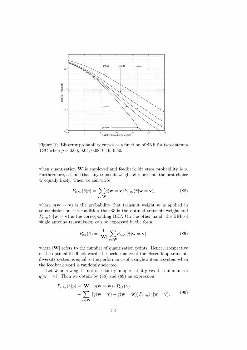
−5 0 5 10 15 20 2510

−4

10−3

10−2

10−1

Bit

Err

or P

roba

bilit

y

SNR Per Bit and Antenna [dB]

p=0.50 p=0.16 p=0.08

p=0.04

p=0.00

Figure 10: Bit error probability curves as a function of SNR for two-antennaTSC when p = 0.00, 0.04, 0.08, 0.16, 0.50.

when quantization W is employed and feedback bit error probability is p.Furthermore, assume that any transmit weight w represents the best choicew equally likely. Then we can write

Pe,Mt(γ|p) =∑

v∈W

q(w = v)Pe,Mt(γ|w = v), (88)

where q(w = v) is the probability that transmit weight w is applied intransmission on the condition that w is the optimal transmit weight andPe,Mt(γ|w = v) is the corresponding BEP. On the other hand, the BEP ofsingle antenna transmission can be expressed in the form

Pe,1(γ) =1|W|

∑

v∈W

Pe,Mt(γ|w = v), (89)

where |W| refers to the number of quantization points. Hence, irrespectiveof the optimal feedback word, the performance of the closed-loop transmitdiversity system is equal to the performance of a single antenna system whenthe feedback word is randomly selected.

Let w be a weight - not necessarily unique - that gives the minimum ofq(w = v). Then we obtain by (88) and (89) an expression

Pe,Mt(γ|p) = |W| · q(w = w) · Pe,1(γ)

+∑

v∈W

(q(w = v)− q(w = w)

)Pe,Mt(γ|w = v). (90)

53

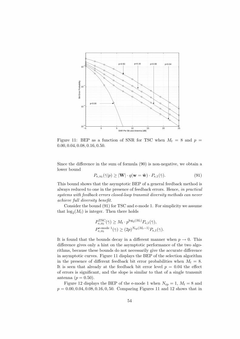
−5 0 5 10 15 20 2510

−4

10−3

10−2

10−1

Bit

Err

or P

roba

bilit

y

SNR Per Bit and Antenna [dB]

p=0.00

p=0.50 p=0.16 p=0.08 p=0.04

Figure 11: BEP as a function of SNR for TSC when Mt = 8 and p =0.00, 0.04, 0.08, 0.16, 0.50.

Since the difference in the sum of formula (90) is non-negative, we obtain alower bound

Pe,Mt(γ|p) ≥ |W| · q(w = w) · Pe,1(γ). (91)

This bound shows that the asymptotic BEP of a general feedback method isalways reduced to one in the presence of feedback errors. Hence, in practicalsystems with feedback errors closed-loop transmit diversity methods can neverachieve full diversity benefit.

Consider the bound (91) for TSC and e-mode 1. For simplicity we assumethat log2(Mt) is integer. Then there holds

PTSCe,Mt

(γ) ≥ Mt · plog2(Mt)Pe,1(γ),

P e-mode 1e,Mt

(γ) ≥ (2p)Nrp(Mt−1)Pe,1(γ).

It is found that the bounds decay in a different manner when p → 0. Thisdifference gives only a hint on the asymptotic performance of the two algo-rithms, because these bounds do not necessarily give the accurate differencein asymptotic curves. Figure 11 displays the BEP of the selection algorithmin the presence of different feedback bit error probabilities when Mt = 8.It is seen that already at the feedback bit error level p = 0.04 the effectof errors is significant, and the slope is similar to that of a single transmitantenna (p = 0.50).

Figure 12 displays the BEP of the e-mode 1 when Nrp = 1, Mt = 8 andp = 0.00, 0.04, 0.08, 0.16, 0, 50. Comparing Figures 11 and 12 shows that in

54

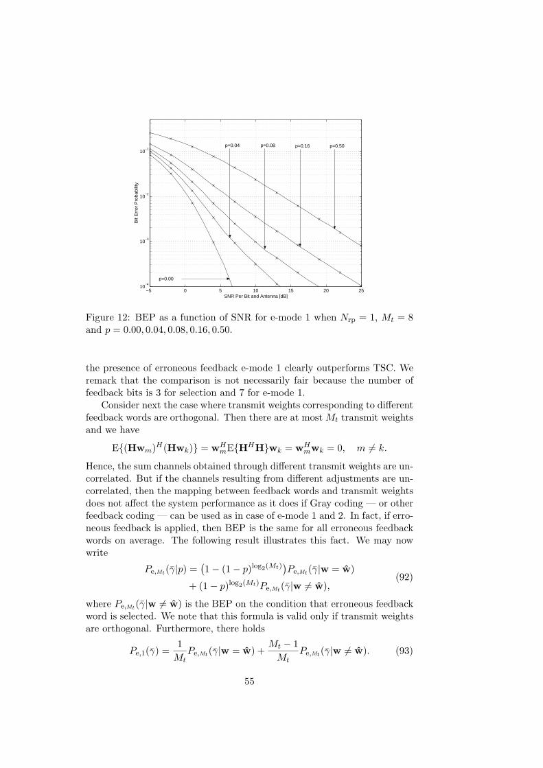
−5 0 5 10 15 20 2510

−4

10−3

10−2

10−1

Bit

Err

or P

roba

bilit

y

SNR Per Bit and Antenna [dB]

p=0.04 p=0.08 p=0.16 p=0.50

p=0.00

Figure 12: BEP as a function of SNR for e-mode 1 when Nrp = 1, Mt = 8and p = 0.00, 0.04, 0.08, 0.16, 0.50.

the presence of erroneous feedback e-mode 1 clearly outperforms TSC. Weremark that the comparison is not necessarily fair because the number offeedback bits is 3 for selection and 7 for e-mode 1.

Consider next the case where transmit weights corresponding to differentfeedback words are orthogonal. Then there are at most Mt transmit weightsand we have

E(Hwm)H(Hwk) = wHmEHHHwk = wH

mwk = 0, m 6= k.

Hence, the sum channels obtained through different transmit weights are un-correlated. But if the channels resulting from different adjustments are un-correlated, then the mapping between feedback words and transmit weightsdoes not affect the system performance as it does if Gray coding — or otherfeedback coding — can be used as in case of e-mode 1 and 2. In fact, if erro-neous feedback is applied, then BEP is the same for all erroneous feedbackwords on average. The following result illustrates this fact. We may nowwrite

Pe,Mt(γ|p) =(1− (1− p)log2(Mt)

)Pe,Mt(γ|w = w)

+ (1− p)log2(Mt)Pe,Mt(γ|w 6= w),(92)

where Pe,Mt(γ|w 6= w) is the BEP on the condition that erroneous feedbackword is selected. We note that this formula is valid only if transmit weightsare orthogonal. Furthermore, there holds

Pe,1(γ) =1

MtPe,Mt(γ|w = w) +

Mt − 1Mt

Pe,Mt(γ|w 6= w). (93)

55

By combining (92) and (93) we obtain

Pe,Mt(γ|p) =(1− Mt

Mt − 1(1− p)log2(Mt)

)Pe,Mt(γ|w = w)

+Mt

Mt − 1(1− p)log2(Mt)Pe,1(γ).

(94)

Thus, when feedback words are orthogonal BEP can be expressed in termsof the BEP of error-free system and BEP of a single antenna transmission.It is worth noticing that BEP of the single antenna transmission dominateswhen SNR is large. Then the term Mt/(Mt − 1)(1 − p)log2(Mt) defines theasymptotic BEP gain of transmit diversity against the single antenna trans-mission.

56

4 Physical Layer Scheduling on a Shared Link

The research of multi-user diversity was initialized in [41], [42] and [72].The goal in multi-user diversity is to provide diversity gain against channelfading through scheduled transmissions. Hence, access to the transmissionresources is granted to users with good channel conditions. If the users arestationary, time selectivity can be introduced artificially as shown in [72].

In Sections 4.2 - 4.5 we compare the capacity of shared links that applylong-term fair scheduling strategies and focus on FDD downlink systems,where channel-aware schedulers require fast feedback channel from mobileto base to allocate transmit resources. The aim is to study practical systemsthat need little control signaling overhead and maintain a simple receiverimplementation. We compare on-off scheduling (OOS) to round robin andmaximum SNR schedulers which provide lower and upper bounds to thescheduling performance, respectively. On-off scheduling requires only one-bit channel quality indicator (CQI), which is a valuable feature, because ithas been observed that the feedback required by maximum SNR schedulercan cause a significant interference, especially when the mobiles are locatedon cell edges [40]. Capacity gains of the three schedulers are derived to-gether with transmitter selection combining (TSC). The effect of limitedfeedback has also been considered in [73], [74] and [76] while the interac-tion of transmit diversity and scheduling has been investigated in [77], [78]and [79].

Fairness is one of the main concerns in the design of scheduling algo-rithms. There is no unique definition for fairness, but usually it is definedfor some low-level characteristic like throughput. Proportional fair sched-uler achieves fairness by transmitting to a user whose instantaneous channelquality is high relative to its own average channel condition over the timescale tc. Thus, in time slot t the proportional fair scheduler transmits to theuser k∗ given by

k∗ = arg maxk

Rk(t)Tk(t)

where Rk(t) is the requested data rate according to the CQI of user k intime slot t and Tk(t) is the average throughput of user k in a past window oflength tc. Alternatively, it is possible to feed back some other metric thanRk(t), such as the received SNR, describing the quality of the connection.Typically, the average throughput Tk(t) is evaluated using an exponentiallyweighted low-pass filter

Tk(t + 1) =

(1− 1/tc)Tk(t) + Rk(t)/tc, k = k∗,(1− 1/tc)Tk(t), k 6= k∗. (95)

When tc is large, the scheduler can wait a long time until transmitting to auser whose channel quality attains a peak. Unfortunately, it is difficult to

57

describe the performance of the proportional fair scheduler in closed-form,because of the filtering operation in (95).

Scheduling based on requested data rates only would be unfair, becauseit would strongly favor the users close to the base station. However, whenrequested data rates are normalized by their respective average through-puts, a scheduling algorithm is fair. In comparisons of Sections 4.2 - 4.5 thelong-term fairness is achieved by reporting a SNR threshold relative to meanreceived SNR, which removes the effect of different path losses due to differ-ent locations of users. We derive asymptotic expression for capacity gains ofthe three systems together with TSC and study the effect of feedback errors.Such errors could be avoided with strong forward error correcting codes, butthis is not a favorable solution when small overheads and feedback latenciesare desired.

Capacity of OOS is studied in Sections 4.2 - 4.5 based on the resultsin [17]. In Section 4.6, BEP in the presence of OOS is considered usingresults of [18] and in Section 4.7 the effect of feedback quantization is in-vestigated [19]. References [20], [21], [22], [23] and [24] provide additionalinformation.

4.1 System Model

The transmission system is shown in Figure 13, where a single data link,transmitted by the base station, is shared between K mobile users. Further-more, a MISO system is assumed, where BS is equipped with Mt transmitantennas, each mobile station has a single receive antenna and it is assumedthat mobile stations are able to estimate the Mt different channels fromthe common pilot signals multiplexed to the data. Such a common codemultiplexed pilot structure is employed, for example, in FDD WCDMA sys-tem [35]. Moreover, we assume that the Mt channels are uncorrelated blockflat Rayleigh fading channels which remain constant during each transmis-sion time interval (TTI) and channel coefficients between separate TTIs areindependent.

As with HSDPA fast PC is not applied. However, slow PC can be used tocompensate shadow fading. Our analysis covers the following two alternativeapproaches:

PC1. Base station applies slow PC so that all K users experience identicallong-term and short-term channel statistics.

PC2. Mean received SNR, denoted by γ, of different users may vary butshort-term statistics of relative SNR γ/γ is the same for all users.

The important common property for PC1 and PC2 is that the schedulingdecision is based on the relative SNR in both approaches. In practice, thetwo approaches, however, will lead to systems of very different nature.

58

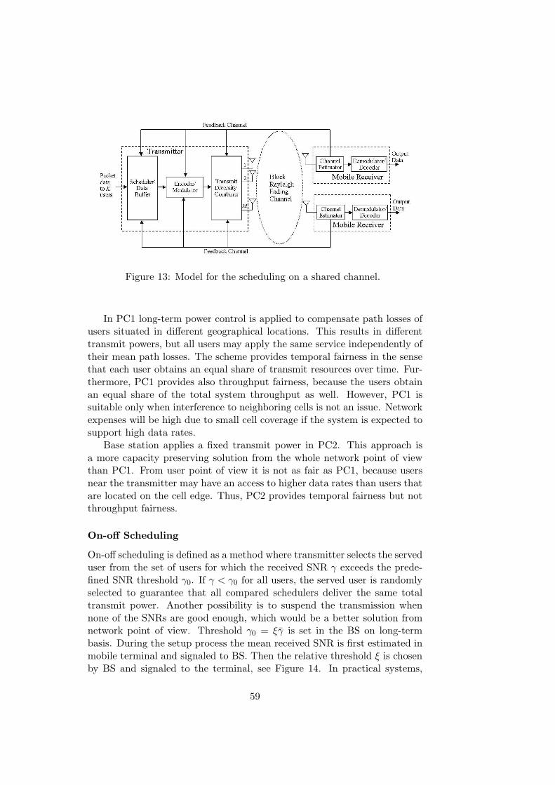
Figure 13: Model for the scheduling on a shared channel.

In PC1 long-term power control is applied to compensate path losses ofusers situated in different geographical locations. This results in differenttransmit powers, but all users may apply the same service independently oftheir mean path losses. The scheme provides temporal fairness in the sensethat each user obtains an equal share of transmit resources over time. Fur-thermore, PC1 provides also throughput fairness, because the users obtainan equal share of the total system throughput as well. However, PC1 issuitable only when interference to neighboring cells is not an issue. Networkexpenses will be high due to small cell coverage if the system is expected tosupport high data rates.

Base station applies a fixed transmit power in PC2. This approach isa more capacity preserving solution from the whole network point of viewthan PC1. From user point of view it is not as fair as PC1, because usersnear the transmitter may have an access to higher data rates than users thatare located on the cell edge. Thus, PC2 provides temporal fairness but notthroughput fairness.

On-off Scheduling

On-off scheduling is defined as a method where transmitter selects the serveduser from the set of users for which the received SNR γ exceeds the prede-fined SNR threshold γ0. If γ < γ0 for all users, the served user is randomlyselected to guarantee that all compared schedulers deliver the same totaltransmit power. Another possibility is to suspend the transmission whennone of the SNRs are good enough, which would be a better solution fromnetwork point of view. Threshold γ0 = ξγ is set in the BS on long-termbasis. During the setup process the mean received SNR is first estimated inmobile terminal and signaled to BS. Then the relative threshold ξ is chosenby BS and signaled to the terminal, see Figure 14. In practical systems,

59

Figure 14: Signaling between base and mobile stations in on-off scheduling.

threshold ξ would be service-specific but since the range of different servicesmay be large, which would lead to unnecessary system complexity, we willemploy the same ξ for all users in examples.

Since γ and ξ are signaled on long-term basis, the corresponding signalingoverhead is small. On the contrary the acknowledgement (ACK) that carriesinstantaneous OOS information needs to be signaled on short-term basis.Fortunately, the information consists of one bit per TTI and again, thesignaling overhead is small when compared to full SNR feedback. If OOS isapplied on top of TSC, terminal monitors Mt channels, defines the largestchannel power and sends the corresponding antenna index together with theone-bit scheduling information to the BS, see Figure 14.

Only scarce channel information is available to BS in OOS. Accordingto this information users can be divided into two groups and the served useris selected from the group of users for which γ > γ0. We could also assume2κ-state quantization with κ-bit scheduling feedback. Then we could divideactive users into 2κ sets and select the user from the set with the highestreceived SNR. When the number of quantization sets grows to infinity weobtain an ideal case where SNR of each user is perfectly known in the BS.In the analysis we will consider only extreme cases where received SNR isnot known in BS, there is one-bit scheduling information, or SNRs of allusers are perfectly known in BS. The feedback channel is similar to thatwith the transmit diversity system in Section 3. Finally, we note that theeffect of feedback latency is neglected, which is approximately valid withinlow mobility environments.

Analyzed Systems

We compare three adaptive systems where the channel is assumed to beperfectly known in the receiver, but the amount of CSI in the transmittervaries.

60

System 1) TSC and round robin. This is a baseline system where theserved user is randomly selected among K active users, or the selection isperformed according to a fixed sequence. The system does not take into ac-count users’ channel states, but there is a user-specific feedback concerningantenna selection. Feedback may be corrupted and the probability of feed-back bit error is denoted by p. Antenna selection feedback consists of theindex of the best transmit antenna only, and it is not useful from schedulingpoint of view.

System 2) TSC and OOS. In OOS, the served user is selected randomly oraccording to a fixed sequence among the users that have reported a positiveACK. If negative acknowledgement (NACK) is received from all users, theserved user is randomly chosen among all active users. Hence, OOS takesinto account the channel state between users in a very simple way: Usersare divided into two groups according to one-bit feedback information andthe served user is selected from the group of users with favorable feedbackbit. The ACK/NACK decision is made in terminal based on the relativeSNR γ/γ. Probability of ACK/NACK error in OOS is denoted by q.

System 3) TSC and maximum SNR scheduling. Here we assume thatBS knows the relative SNR of the best channel out of Mt alternatives. Thus,terminal reports unquantized relative SNR γ/γ, where γ is the SNR of thestrongest channel, to BS, and the user with the best relative SNR is served.

Comparison

The primary intention of the comparison is not to provide absolute perfor-mance results, but instead, we adopt the following two goals using capacityof the shared link as a performance measure:

• Investigate the effect of relative SNR feedback to the system performance.

• Track the effect of feedback errors.

For the first goal we make a comparison between systems 1-3, but forthe second goal we only investigate systems 1 and 2. Although it is knownthat system capacity in SISO channels is maximized when all resources aregiven to the user with the best absolute SNR, we study systems where CSIin the transmitter is based on the relative SNR, because it provides a goodstarting point when designing practical and ’more fair’ scheduling strategiesthan the conventional maximum SNR scheduling.

Fast power control is not applied on the shared channel and in perfor-mance comparisons we can apply the channel capacity assuming constanttransmit power and optimal rate adaptation to the channel fading. Thus,

Cl(γ) = B · Elog2(1 + γ)|system l. (96)

61

Capacities of the different systems can then be obtained by using corre-sponding SNR distributions.

Finally, we note that the mean user capacities in systems 1-3 are simplygiven by Cl/K, l = 1, 2, 3, provided that there are K active users. Whiledelay can be fixed in system 1 to K TTIs, in systems 2 and 3 the delayvaries, the expectation being the same K TTIs. In practice, the variationof the delay depends on queueing principles of the schedulers and type ofservices.

4.2 Round Robin Scheduling with TSC

Closed-form capacity formulas for receiver selection combining have beenpreviously considered in [54], and the results are directly applicable alsoto TSC provided that error-free feedback is available. Since this is notnecessarily the case in system 1 we extend the capacity analysis to coverTSC with corrupted feedback.

Probability Density Function

We begin by recalling the distribution of the received SNR after error-freetransmitter selection combining over Mt antennas,

fTSC(γ) =Mt

γ· e−γ/γ

(1− e−γ/γ

)Mt−1. (97)

For the SNR distribution of system 1 it remains to model the effect offeedback errors. For this purpose we recall the model in Section 3.5, andassume for simplicity that Mt = 2κ, κ ∈ N so that the uncoded feedbackword in TSC contains κ bits. Following the reasoning of (92), (93) and (94)we find that the PDF of received SNR in system 1 - denoted by f1 - can bewritten as

f1(γ) =(1− Mtpw

Mt − 1

)fTSC(γ) +

Mtpw

Mt − 1fSA(γ), (98)

where pw = 1−(1−p)κ, κ = log2(Mt), is the feedback word error probabilityand fSA is the PDF corresponding to the single antenna transmission. Hence,the PDF of SNR for TSC with corrupted feedback can be expressed in termsof PDF of SNR for TSC without feedback errors and PDF corresponding tosingle antenna transmission.

Computation of Capacity

Capacity for system 1 can be computed using (96) and (98). For that pur-pose we recall from [54] the capacity formula for TSC over Mt antennas. We

62

0 0.1 0.2 0.3 0.4 0.5 1

2

3

4

5

Feedback bit error probability

Cap

acity

[Bits

/Sec

/Hz]

Figure 15: Capacity of system 1 as a function of feedback bit error proba-bility when SNR = 2 dB (solid curves), SNR = 10 dB (dashed curves) andMt = 1 (-∇-), Mt = 2 (-*-), Mt = 4 (-o-) and Mt = 8 (-x-).

have

CTSC(γ) = B · log2(e)Mt∑

m=1

(Mt

m

)(−1)m−1em/γE1

(m/γ

). (99)

The required capacity for single antenna transmission - denoted by CSA - overRayleigh fading channel is obtained from (99) by setting Mt = 1. By (98)and (99) we obtain

C1(γ) =(1− Mtpw

Mt − 1

)CTSC(γ) +

Mtpw

Mt − 1CSA(γ). (100)

Figure 15 depicts the capacity of system 1 as a function of feedbackbit error probability when SNR is 2 and 10 dB, and Mt = 1, 2, 4, 8. It isfound that the adverse effect of feedback errors increases with the number oftransmit antennas. This is due to the fact that for fixed bit error probabilitythe feedback word error probability increases rapidly when the length of thefeedback word is growing. Hence, if the number of transmit antennas islarge, uncoded feedback is a suitable choice only if the bit error probabilityon the feedback channel is small.

Figure 15 also hints that capacity gain from TSC increases with SNR.However, the gain will saturate when SNR becomes large. To show this wededuce the formula

C1(γ) = CSA(γ) +(1− Mtpw

Mt − 1

)∆1(γ), (101)

63

where ∆1 is the selection gain over Mt antennas, given by

∆1(γ) ≈ B ·Mt∑

m=1

(Mt

m

)(−1)m log2(m), γ >> 1. (102)

Through this formula it is found that in high SNR region selection gaindepends only on the number of antennas. Furthermore, feedback errorsreduce the achievable gain and the gain vanishes when p = 0.5.

Let us now show (101)– (102). From (100) we obtain

C1(γ)−CSA(γ) =(1− Mtpw

Mt − 1

)(CTSC(γ)−CSA(γ)

). (103)

The difference on the right hand side represents the gain of TSC when feed-back is error-free. At this stage we recall that exponential integral functionadmits the expression [69]

E1(x) = −e0 − log(x)−∞∑

n=1

(−x)n

n · n!, (104)

where e0 = 0.5772156649 refers to Euler constant. If x is small, we mayneglect the sum term and approximate

E1(x) ≈ −e0 − log(x), x << 1. (105)

By (103) we have ∆1 = CTSC(γ)−CSA(γ) and if γ >> 1, we find from (99)and (105) that

∆1(γ) ≈ B · log2(e)Mt∑

m=1

(Mt

m

)(−1)m

(e0 + log(m/γ)

)

+ B log2(e)(e0 + log(1/γ)

).

(106)

Here we can apply the equation

Mt∑

m=1

(Mt

m

)(−1)m = −1 (107)

that can be easily shown to be valid by binomial expansion. Equation (102)is now obtained by (106) and (107), and (101) follows by (103).

4.3 On-off Scheduling with TSC

In order to avoid unnecessary complexity in the analysis of system 2 weneglect the effect of TSC errors and concentrate on OOS errors. However,incorporating TSC errors to the analysis is a straightforward extension.

64

Probability Density Function

Assume first an error-free feedback and let P+ be the probability that a usersends an ACK, and P+ = 1 − P−, where P− is the probability of NACK.Then, in system 2 the PDF of SNR on the shared channel attains the form

f2(γ) = (1− PK− )f2(γ|I+) + PK

− f2(γ|I−), (108)

where 1−PK− is the probability that γ ∈ I+ = (γ0,∞) for some of the usersand PK− indicates that γ ∈ I− = (0, γ0] for all users. Without feedbackerrors the conditional PDFs are of the form

f2(γ|I±) = u±(γ)fTSC(γ)/P±, (109)

where u± is the step function such that

u+(γ) =

1, γ > γ0

0, γ ≤ γ0

, u−(γ) = 1− u+(γ). (110)

It will turn out that the capacity of system 2 can be expressed in termsof a certain ACK probability that is further related to threshold ξ throughthe equation

P+ = 1− FTSC(γ0) = 1− (1− e−ξ)Mt , (111)

where FTSC refers to the cumulative distribution function (CDF) of TSC.Hence, it is found that

ξ = − log(1− (1− P+)1/Mt

). (112)

This formula can be used when illustrating the capacity of system 2 as afunction of ACK probability.

It is assumed that terminal compares the received SNR to a thresholdwithout errors, but feedback errors may corrupt decisions made in the BS.If ACK/NACK information is corrupted, we have

f2,q(γ|I±) =(1− q) · u±(γ) + q · u∓(γ)

(1− q) · P± + q · P∓ fTSC(γ), (113)

where q is the ACK/NACK error probability and the denominator gives theACK/NACK probability in BS in the presence of feedback errors. There aretwo possible events leading to positive ACK decision in BS: The receivedSNR in terminal is above the given threshold and the received feedback inBS is correct, or the received SNR is below the threshold but the feedbackis corrupted and BS receives ACK. Analogously, NACK decision in BS mayprecede two similar but complementary events. We write

P±,q = (1− q) · P± + q · P∓ = q + (1− 2q) · P±, (114)

65

and after some simple manipulations we obtain

f2,q(γ|I±) =(1− 2q) · P±f2(γ|I±)

P±,q+

q · fTSC(γ)P±,q

. (115)

The PDF of SNR in case of system 2 with corrupted feedback is given by

f2,q(γ) = (1− PK−,q)f2,q(γ|I+) + PK

−,q · f2,q(γ|I−). (116)

Computation of Capacity

From (115) it is found that capacity for system 2 can be deduced providedthat conditional capacities can be computed. Using (109) we obtain

C2(γ|I+) =B · log2(e)

P+

∫ ∞

γ0

log(1 + γ)fTSC(γ)dγ. (117)

After applying the integration by parts it is found that

C2(γ|I+) =B · log2(e)

P+

(P+ log(1 + γ0) +

∫ ∞

γ0

1− FTSC(γ)1 + γ

dγ). (118)

In (118) we apply the equality

FTSC(γ) =Mt∑

m=0

(Mt

m

)(−1)me−mγ/γ (119)

that is found by binomial expansion. Before combining the last two equa-tions we give the formula

∫ ∞

γ0

e−mγ/γ

1 + γdγ = em/γE1((1 + γ0)m/γ) (120)

that results after using the substitution (1 + γ)m/γ → γ. The formula forconditional capacity (117) is achieved by combining (118), (119) and (120).We have

C2(γ|I+) =B · log2(e)

P+

(P+ log(1 + γ0)

+Mt∑

m=1

(Mt

m

)(−1)m−1em/γE1

((1 + γ0)m/γ

)).

(121)

Furthermore, in case of feedback errors there holds

C2,q(γ|I±) =(1− 2q) · P±C2(γ|I±)

P±,q+

q · CTSC(γ)P±,q

. (122)

66

For the final capacity formula we also need the capacity on the conditionthat γ ≤ γ0. For that purpose we note that

C2(γ|I−) =1

P−

(CTSC(γ)− P+C2(γ|I+)

). (123)

Capacity of system 2 is obtained using (116), (115) and (121) - (123).Let us suppose an extreme case where K →∞. This case is interesting

because it provides an upper bound for the achievable capacity in system 2.Now, for any threshold γ0 there exists a user with γ > γ0. Hence, with ’+’equation (122) defines the capacity of system 2. Moreover, we have

C2,q(γ|I+) ≥ (1− 2q)P+

q + (1− 2q)P+C2(γ|I+)

≥ (1− 2q)P+

q + (1− 2q)P+CAWGN(ξγ),

(124)

where the latter estimate follows from (118) because the integral termin (118) is positive and can be dropped out from (124).

Assume for a while that the mean SNR is fixed. If q 6= 0, then (124) givesonly a trivial bound when P+ → 0, but if there are no feedback errors, thelower bound in (124) grows without limit when P+ → 0. Although (124)hints that large capacity gains can be achieved on the shared channel ifthe number of active users is large, the capacities of individual users decay,because there is an increasing number of users competing simultaneously onthe same shared channel resource.

This phenomenon is illustrated in Figure 16, which shows the capacityof system 2 as a function of ACK probability when K →∞. It is found thatthe effect of feedback errors is largest when ACK probability is small. Thisis due to the fact that the error event where BS transmits although terminalsent NACK begins to dominate when P+ is small. Then it might evenhappen that most of the packets are transmitted at a wrong time. Hence,the expected P+ should be taken into account in the design of the feedbackchannel. Finally, we note that the effect of scheduling errors is smaller incase of four transmit antennas than in case of one transmit antenna, becauseoverall gain of OOS is smaller when also TSC is applied.

Assume next a finite number of users and a fixed probability of ACK.Then we may write

C2(γ) = CSA(γ) + ∆2(γ), (125)

where ∆2 represents the gain of system 2 versus continuous single antennatransmission. Let us compute this gain. For simplicity we neglect the effectof feedback errors. Then, by using (123) we obtain

C2(γ) = (1− PK− )C2(γ|I+) + PK

− C2(γ|I−)

= (1− PK−1− )C2(γ|I+) + PK−1

− CTSC(γ).(126)

67

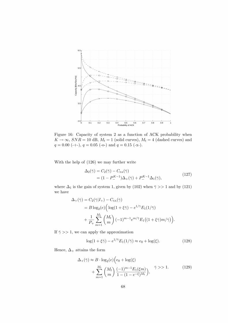
0 0.1 0.2 0.3 0.4 0.5 0.6 0.7 0.8 0.9 12.5

3.5

4.5

5.5

6.5

Probability of ACK

Cap

acity

[Bits

/Sec

/Hz]

Figure 16: Capacity of system 2 as a function of ACK probability whenK →∞, SNR = 10 dB, Mt = 1 (solid curves), Mt = 4 (dashed curves) andq = 0.00 (-+-), q = 0.05 (-o-) and q = 0.15 (-x-).

With the help of (126) we may further write

∆2(γ) = C2(γ)− CSA(γ)

= (1− PK−1− )∆+(γ) + PK−1

− ∆1(γ),(127)

where ∆1 is the gain of system 1, given by (102) when γ >> 1 and by (121)we have

∆+(γ) = C2(γ|I+)− CSA(γ)

= B log2(e)(

log(1 + ξγ)− e1/γE1(1/γ)

+1

P+

Mt∑

m=1

(Mt

m

)(−1)m−1em/γE1

((1 + ξγ)m/γ

)).

If γ >> 1, we can apply the approximation

log(1 + ξγ)− e1/γE1(1/γ) ≈ e0 + log(ξ). (128)

Hence, ∆+ attains the form

∆+(γ) ≈ B · log2(e)(e0 + log(ξ)

+Mt∑

m=1

(Mt

m

)(−1)m−1E1(ξm)1− (1− e−ξ)Mt

),

γ >> 1. (129)

68

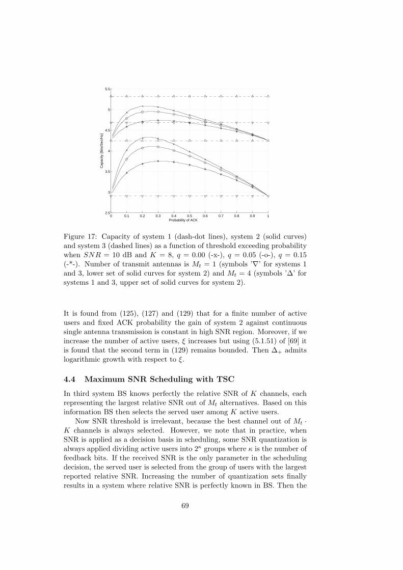
0 0.1 0.2 0.3 0.4 0.5 0.6 0.7 0.8 0.9 12.5

3

3.5

4

4.5

5

5.5

Probability of ACK

Cap

acity

[Bits

/Sec

/Hz]

Figure 17: Capacity of system 1 (dash-dot lines), system 2 (solid curves)and system 3 (dashed lines) as a function of threshold exceeding probabilitywhen SNR = 10 dB and K = 8, q = 0.00 (-x-), q = 0.05 (-o-), q = 0.15(-*-). Number of transmit antennas is Mt = 1 (symbols ’∇’ for systems 1and 3, lower set of solid curves for system 2) and Mt = 4 (symbols ’∆’ forsystems 1 and 3, upper set of solid curves for system 2).

It is found from (125), (127) and (129) that for a finite number of activeusers and fixed ACK probability the gain of system 2 against continuoussingle antenna transmission is constant in high SNR region. Moreover, if weincrease the number of active users, ξ increases but using (5.1.51) of [69] itis found that the second term in (129) remains bounded. Then ∆+ admitslogarithmic growth with respect to ξ.

4.4 Maximum SNR Scheduling with TSC

In third system BS knows perfectly the relative SNR of K channels, eachrepresenting the largest relative SNR out of Mt alternatives. Based on thisinformation BS then selects the served user among K active users.

Now SNR threshold is irrelevant, because the best channel out of Mt ·K channels is always selected. However, we note that in practice, whenSNR is applied as a decision basis in scheduling, some SNR quantization isalways applied dividing active users into 2κ groups where κ is the number offeedback bits. If the received SNR is the only parameter in the schedulingdecision, the served user is selected from the group of users with the largestreported relative SNR. Increasing the number of quantization sets finallyresults in a system where relative SNR is perfectly known in BS. Then the

69

2 3 4 5 6 7 8 9 102.5

3

3.5

4

4.5

5

5.5

Number of active users

Cap

acity

[Bits

/Sec

/Hz]

Figure 18: Capacity of system 1 (dash-dot lines), system 2 (solid and dottedcurves) and system 3 (dashed curves) when SNR = 10 dB, q = 0.00 (-x-),q = 0.05 (-o-) and q = 0.15 (-*-) as a function of active users. The numberof transmit antennas is Mt = 1 (symbols ’∇’ for systems 1 and 3, set of solidcurves for system 2) and Mt = 4 (symbols ’∆’ for systems 1 and 3, set ofdotted curves for system 2). System 2 applies optimal ACK probability.

PDF of SNR on the shared channel is given by

f3(γ) = K · fTSC(γ)FTSC(γ)K−1 = Mt ·K · fSA(γ)FSA(γ)Mt·K−1.

The capacity of the shared link is now obtained from (99) by substitutingMt ·K to Mt. Feedback errors are not modelled because there is no quanti-zation. Finally, we note that asymptotic formula similar to (101) and (102)can be easily deduced for system 3 as well. The corresponding gain of sys-tem 3 against continuous single antenna transmission is denoted by ∆3 andaccording to (102) we have

∆3(γ) ≈ B ·Mt·K∑

m=1

(Mt ·K

m

)(−1)m log2(m), γ >> 1.

4.5 Comparisons and Conclusions

We begin the comparison from Figure 17, which shows the capacities ofsystems 1-3 as a function of ACK probability when SNR=10 dB, K = 8,and the curves are based on closed-form formulas of the previous sections.

70

0 2 4 6 8 10 12 14 16 18 200.2

0.3

0.4

0.5

Average received SNR [dB]

Opt

imal

AC

K p

roba

bilit

y

Figure 19: Optimal ACK probability in system 2 as a function of mean SNRwhen Mt = 1 (-x-), Mt = 4 (-o-) and the numbers of active users are 2 (solidcurves), 4 (dashed curves) and 8 (dash-dot curves).

As was already noticed from the asymptotic formula of ∆2, the capacityof system 2 varies with the ACK probability, and Figure 17 shows thatthere exists an ACK probability which maximizes capacity. With error-freefeedback and single transmit antenna the difference between capacities ofsystem 2 and 3 is only round 0.5 bits/sec/Hz when applying optimal ACKprobability. On the other hand, at this optimal point the capacity differencebetween systems 1 and 2 is slightly less than 1.5 bits/sec/Hz. Hence, withOOS it is possible to achieve round G = 75% of the gain of relative SNRfeedback, where the relative gain of OOS is defined as

G =C2 − C1

C3 − C1· 100%.

Note that we measure the gain of OOS with respect to round robin, whilethe 90% gain in [74] refers to percentage of the maximum SNR schedulinggain. Approximately the same ratio applies with four transmit antennasbut the absolute gains are smaller. In fact, if the number of active users isfixed but the number of transmit antennas increases, the lower and upperbounds for the capacity of system 2, defined by capacities of systems 1 and3, respectively, are closing and achievable scheduling gain is decreasing. Inhigh SNR region, this difference can be computed from (102).

We also find from Figure 17 that the effect of scheduling errors is re-markable but not as dramatic as in Figure 16 where feedback errors becomea dominating factor when ACK probability is small. Thus, the results point

71

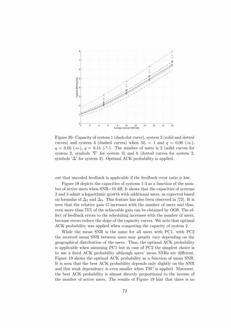
0 2 4 6 8 10 12 14 16 18 200

1

2

3

4

5

6

7

8

Average received SNR [dB]

Cap

acity

[Bits

/Sec

/Hz]

Figure 20: Capacity of system 1 (dash-dot curve), system 2 (solid and dottedcurves) and system 3 (dashed curves) when Mt = 1 and q = 0.00 (-x-),q = 0.05 (-o-), q = 0.15 (-*-). The number of users is 2 (solid curves forsystem 2, symbols ’∇’ for system 3) and 8 (dotted curves for system 2,symbols ’∆’ for system 3). Optimal ACK probability is applied.

out that uncoded feedback is applicable if the feedback error ratio is low.Figure 18 depicts the capacities of systems 1-3 as a function of the num-

ber of active users when SNR=10 dB. It shows that the capacities of systems2 and 3 admit a logarithmic growth with additional users, as expected basedon formulas of ∆2 and ∆3. This feature has also been observed in [72]. It isseen that the relative gain G increases with the number of users and thus,even more than 75% of the achievable gain can be obtained by OOS. The ef-fect of feedback errors to the scheduling increases with the number of users,because errors reduce the slope of the capacity curves. We note that optimalACK probability was applied when computing the capacity of system 2.

While the mean SNR is the same for all users with PC1, with PC2the received mean SNR between users may greatly vary depending on thegeographical distribution of the users. Thus, the optimal ACK probabilityis applicable when assuming PC1 but in case of PC2 the simplest choice isto use a fixed ACK probability although users’ mean SNRs are different.Figure 19 shows the optimal ACK probability as a function of mean SNR.It is seen that the best ACK probability depends only slightly on the SNRand this weak dependency is even smaller when TSC is applied. Moreover,the best ACK probability is almost directly proportional to the inverse ofthe number of active users. The results of Figure 19 hint that there is no

72

large penalty when fixed ACK probability and the corresponding thresholdξ are applied to the whole SNR scale.

Figure 20 displays the capacities of systems 1-3 as a function of meanSNR when optimal ACK probability is applied. We note that the resultswould have been practically the same, up to figure resolution, if fixed ACKprobability, optimal for SNR=10 dB, had been applied to the whole SNRscale. Hence the results of Figure 20 are valid for both PC1 and PC2. It isworth mentioning that the gains of systems 2 and 3 against system 1 remainnoticeable also when SNR is low.

4.6 Computation of Bit Error Probabilities

The goal of this section is to investigate the receiver BEP when OOS isapplied. Results will show that the effect of feedback errors is crucial to thesystem. Without feedback errors the asymptotic decay of BEP is exponentialwhile in the presence of feedback errors the slope of the asymptotic decayof BEP is the same as in case of continuous transmission.

We have adopted the system model from Section 4.1. The only differ-ence is that we now also consider the rate 1 orthogonal space–time blockcoded (STBC) transmission that is available for BPSK modulation whenMt ∈ 2, 4, 8 [49]. In STBC, different code sequences are transmitted fromseparate antennas, and after decoding in the receiver, the received SNR isof the form

γ =1

Mt

Mt∑

m=1

γm.

We remark that the transmit power has been divided evenly between theMt antennas.

General Formulas

The performance of the systems is studied using the bit error probability asa performance measure,

POOSe (γ) = EPmod(γ)| OOS .

We will concentrate in BPSK modulation, but the analysis can be extendedto other MPSK and QAM schemes by utilizing the corresponding BEP ap-proximations [71] or exact expressions [80] for Pmod. Furthermore, bit errorprobabilities for adaptive modulation schemes assuming different switchinglevels can be derived from the given expressions.

We recall that the PDF of SNR in the presence of OOS is defined by

fOOS(γ) = u+(γ)f(γ)/P+,

where u+ is the step function of (110), P+ is the probability of positiveACK in OOS and f refers to the PDF of SNR in the underlying unscheduled

73

system. In this section, f corresponds to single antenna transmission, TSCor STBC.

Assuming that the feedback bit error probability is q, we further recallthat the PDF to be integrated is expressed in the form

fOOSq (γ) =

(1− q) · u+(γ) + q · u−(γ)(1− q) · P+ + q · P− f(γ),

where the denominator gives the transmission probability in the presence ofOOS feedback bit errors.

According to (114) and (115) the PDF attains the form

fOOSq (γ) =

(1− 2q) · P+fOOS(γ)P+,q

+q · f(γ)P+,q

.

Hence, the PDF of the received SNR can be expressed in terms of the PDFof error-free transmission and continuous transmission. This implies thefollowing interesting result on BEP. Namely, BEP in the presence of OOSand feedback bit errors can be written as

POOSe,q (γ) =

(1− 2q) · POOSe (γ)

P+,q+

q · Pe(γ)P+,q

, (130)

where POOSe is the BEP without feedback errors and Pe is the BEP of con-

tinuous transmission.Later we will see that the asymptotic decay of POOS

e is exponential in thethree example cases. Therefore, if γ is high, then Pe will dominate over POOS

e .This implies that the slope of the asymptotic BEP in the logarithmic scale isthe same as in case of continuous transmission, but there is a constant BEPgain of magnitude 10 log10(q/P+,q) at high SNR region. In system design qand P+ should be selected such that feedback errors will not dominate inthe SNR region where the system is operating.

Calculation of Bit Error Probabilities

We evaluate bit error probabilities by simply using the integration by parts.This is possible in the studied cases because the integral functions of distri-butions are known. Moreover, for the BPSK modulation we have

d

dγPmod(γ) = − 1√

4πγe−γ (131)

(see [69] (6.5.17), (7.1.2) and (7.1.19)). This approach provides integralformulas that can be expressed using combinations of complementary in-complete gamma function

Γ(t, x) =∫ ∞

xe−sst−1ds. (132)

74

Single Antenna Transmission. Assume a single antenna transmissionin flat Rayleigh fading environment. Then using (131), and integration byparts we find that the BEP is of the form

POOSe (γ) =

1√4π

(Γ(12, ξγ

)−√

γ

1 + γeξΓ

(12, ξ(1 + γ)

)). (133)

Before [18] a similar formula was presented in [42]. The formula for BEPin the presence of feedback errors can be found directly by using (130).Furthermore, employing (6.5.32) in [69] we obtain the asymptotic formulafor large SNR

POOSe (γ) =

e−ξγ

√4πξγ3

, γ >> 1. (134)

Hence, without feedback errors the asymptotic decay of BEP is exponential.Figure 21 illustrates the performance of the single transmit antenna sys-

tem when P+,q = 0.2. This ACK probability of OOS is rather low and itcan be used only if the number of active users is large. We note that in aK-user system with i.i.d. channels the system outage probability becomes(1 − P+,q)K . The BEP results in this section are given for fixed P+,q. Forthat purpose we solve ξ of (133) from equation

P+,q = q + (1− 2q)P+ = q + (1− 2q)e−ξ.

Then, after substituting the value of ξ into (133) we obtain by (130) BEP asa function of SNR for different values of P+,q. It is seen that BEP decreasesrapidly when SNR is high and there are no feedback errors. Moreover, it isnoticed that feedback errors seriously degrade the performance at high SNR,and the asymptotic behavior of BEP in the presence of feedback errors isclearly visible.

OOS with TSC. In case of TSC, the PDF of SNR is given by (97) andthe effect of antenna selection errors can be taken into account throughformula (98). We note that the asymptotic diversity order is Mt whenantenna selection is error-free and only OOS feedback is subject to errors.However, asymptotic diversity order becomes one when both feedback typesare subject to feedback errors.

A closed-form expression for the BEP is deduced employing the inte-gration by parts. This is possible because the integral function of fTSC isknown. Furthermore, applying the binomial expansion to the expression(1− e−γ/γ)M we obtain

POOSe (γ) =

1√4π

(Γ(12, ξγ

)+

Mt∑

m=1

(Mt

m

)√γ

m + γ

(−1)mΓ(

12 , ξ(m + γ

)

1− (1− e−ξ)Mt

).

This equation provides the BEP of OOS when TSC is used and feedbackinformation is error-free. Again, employing (6.5.32) in [69] we find that for

75

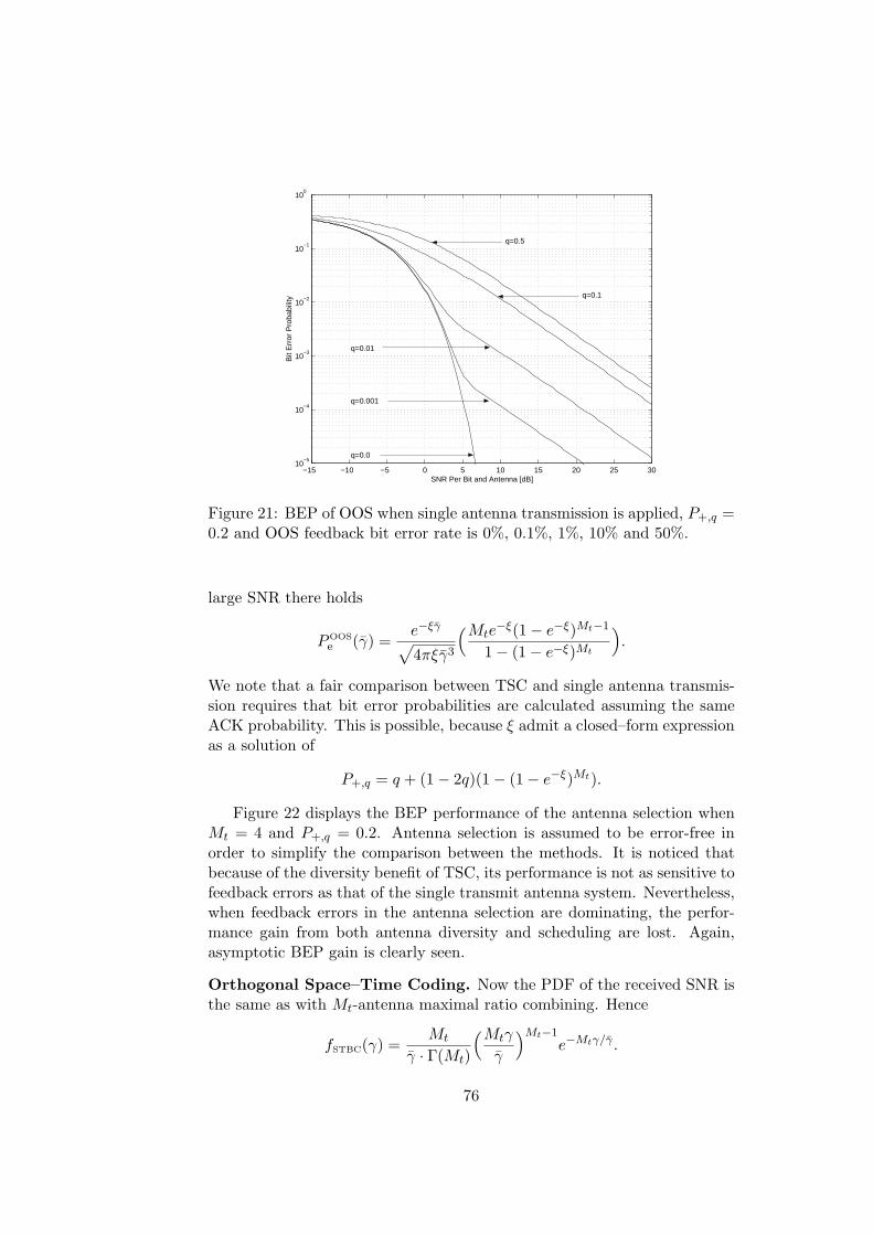
−15 −10 −5 0 5 10 15 20 25 3010

−5

10−4

10−3

10−2

10−1

100

Bit

Err

or P

roba

bilit

y

SNR Per Bit and Antenna [dB]

q=0.001

q=0.01

q=0.0

q=0.5

q=0.1

Figure 21: BEP of OOS when single antenna transmission is applied, P+,q =0.2 and OOS feedback bit error rate is 0%, 0.1%, 1%, 10% and 50%.

large SNR there holds

POOSe (γ) =

e−ξγ

√4πξγ3

(Mte−ξ(1− e−ξ)Mt−1

1− (1− e−ξ)Mt

).

We note that a fair comparison between TSC and single antenna transmis-sion requires that bit error probabilities are calculated assuming the sameACK probability. This is possible, because ξ admit a closed–form expressionas a solution of

P+,q = q + (1− 2q)(1− (1− e−ξ)Mt).

Figure 22 displays the BEP performance of the antenna selection whenMt = 4 and P+,q = 0.2. Antenna selection is assumed to be error-free inorder to simplify the comparison between the methods. It is noticed thatbecause of the diversity benefit of TSC, its performance is not as sensitive tofeedback errors as that of the single transmit antenna system. Nevertheless,when feedback errors in the antenna selection are dominating, the perfor-mance gain from both antenna diversity and scheduling are lost. Again,asymptotic BEP gain is clearly seen.

Orthogonal Space–Time Coding. Now the PDF of the received SNR isthe same as with Mt-antenna maximal ratio combining. Hence

fSTBC(γ) =Mt

γ · Γ(Mt)

(Mtγ

γ

)Mt−1e−Mtγ/γ .

76

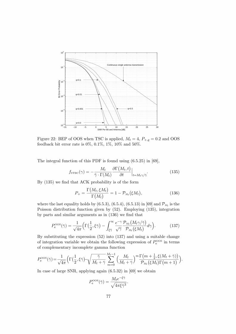
−15 −10 −5 0 5 10 15 20 25 3010

−5

10−4

10−3

10−2

10−1

100

Bit

Err

or P

roba

bilit

y

SNR Per Bit and Antenna [dB]

q=0.0

q=0.001

q=0.01

q=0.1

q=0.5

Continuous single antenna transmission

Figure 22: BEP of OOS when TSC is applied, Mt = 4, P+,q = 0.2 and OOSfeedback bit error rate is 0%, 0.1%, 1%, 10% and 50%.

The integral function of this PDF is found using (6.5.25) in [69],

fSTBC(γ) = − Mt

γ · Γ(Mt)∂Γ

(Mt, t

)

∂t

∣∣∣t=Mtγ/γ

. (135)

By (135) we find that ACK probability is of the form

P+ =Γ(Mt, ξMt

)

Γ(Mt

) = 1− PMt

(ξMt

), (136)

where the last equality holds by (6.5.3), (6.5.4), (6.5.13) in [69] and PMt is thePoisson distribution function given by (52). Employing (135), integrationby parts and similar arguments as in (136) we find that

POOSe (γ) =

1√4π

(Γ(12, ξγ

)−∫ ∞

ξγ

e−γ

√γ

PMt

(Mtγ/γ

)

PMt

(ξMt

) dγ). (137)

By substituting the expression (52) into (137) and using a suitable changeof integration variable we obtain the following expression of POOS

e in termsof complementary incomplete gamma function

POOSe (γ)=

1√4π

(Γ(12, ξγ

)−√

γ

Mt + γ

Mt−1∑

m=0

( Mt

Mt + γ

)m Γ(m + 1

2 , ξ(Mt + γ))

PMt

(ξMt

)Γ(m + 1

)).

In case of large SNR, applying again (6.5.32) in [69] we obtain

POOSe (γ) =

Mte−ξγ

√4πξγ3

.

77

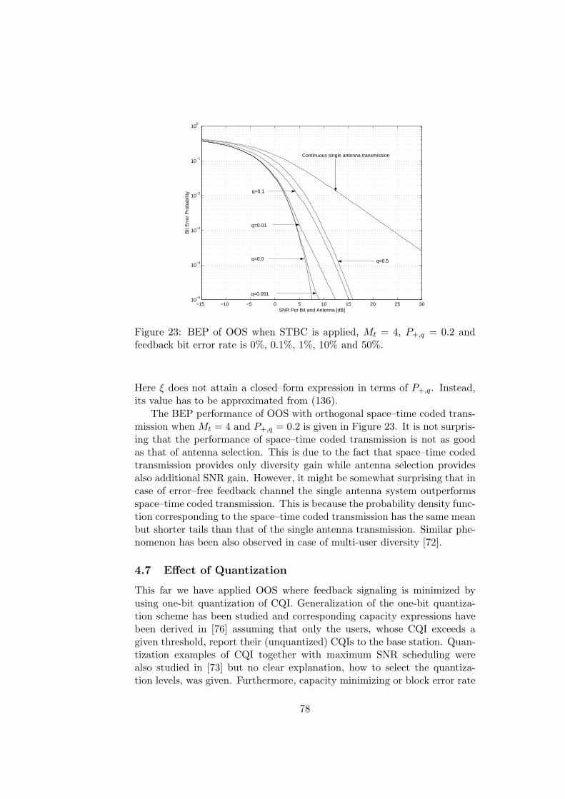
−15 −10 −5 0 5 10 15 20 25 3010

−5

10−4

10−3

10−2

10−1

100

Bit

Err

or P

roba

bilit

y

SNR Per Bit and Antenna [dB]

Continuous single antenna transmission

q=0.001

q=0.0

q=0.01

q=0.1

q=0.5

Figure 23: BEP of OOS when STBC is applied, Mt = 4, P+,q = 0.2 andfeedback bit error rate is 0%, 0.1%, 1%, 10% and 50%.

Here ξ does not attain a closed–form expression in terms of P+,q. Instead,its value has to be approximated from (136).

The BEP performance of OOS with orthogonal space–time coded trans-mission when Mt = 4 and P+,q = 0.2 is given in Figure 23. It is not surpris-ing that the performance of space–time coded transmission is not as goodas that of antenna selection. This is due to the fact that space–time codedtransmission provides only diversity gain while antenna selection providesalso additional SNR gain. However, it might be somewhat surprising that incase of error–free feedback channel the single antenna system outperformsspace–time coded transmission. This is because the probability density func-tion corresponding to the space–time coded transmission has the same meanbut shorter tails than that of the single antenna transmission. Similar phe-nomenon has been also observed in case of multi-user diversity [72].

4.7 Effect of Quantization

This far we have applied OOS where feedback signaling is minimized byusing one-bit quantization of CQI. Generalization of the one-bit quantiza-tion scheme has been studied and corresponding capacity expressions havebeen derived in [76] assuming that only the users, whose CQI exceeds agiven threshold, report their (unquantized) CQIs to the base station. Quan-tization examples of CQI together with maximum SNR scheduling werealso studied in [73] but no clear explanation, how to select the quantiza-tion levels, was given. Furthermore, capacity minimizing or block error rate

78

maximizing quantizations within maximum SNR scheduling were consideredin [74] showing that two-bit quantization obtains 90% of the unquantizedCQI gain in the example scenarios. The quantization regions were foundusing numerical optimization.

In this section we study the quantization of CQI in maximum SNRscheduling. We apply the system model of Section 4.1 and show closed-formexpressions for BEP assuming suboptimal quantization strategy. Resultsare based on [19].

General Formulas

Optimal quantization of relative SNR depends on fading statistics as well asthe selected performance measure. Below we use the bit error probabilityas a performance measure,

PQe (γ) = EPmod(γ)|Q , (138)

where Q refers to the applied quantization. Let us give a general formula-tion of the studied quantization problem: Assume that Q is the set of allquantizations and let Q = ξlL+1

l=0 ,

0 = ξ0 < ξ1 < · · · < ξL+1 = ∞, ξl = γl/γ, (139)

where γl = ξlγ is boundary point of the true SNR quantization. If BEP isused as a performance measure, then the aim is to find Q ∈ Q that minimizethe BEP for a certain bit rate R, i.e.

P Qe (γ) = minPQ

e (γ) : Q ∈ Q, R. (140)

It turns out that the best quantization Q varies with the mean SNR. Hence,the predefined target SNR defines the best quantization.

To this end, we need to compute the object function PQe . Let ql be the

probability that a shared channel is dedicated to a user, whose received SNRis in the interval (γl, γl+1). Then the PDF fQ can be expressed in the form

fQ(γ) =L∑

l=0

ql ·(ul(γ)f(γ)/pl

), (141)

where f refers to the PDF of the SNR in the reference system and

ul(γ)=

1, γ ∈ (γl, γl+1),0, otherwise,

pl =∫ γl+1

γl

f(γ)dγ. (142)

We note that the function in the brackets in (141) is the PDF of the SNR onthe condition that the received reference SNR is in (γl, γl+1). Furthermore,in case of K active users with i.i.d. statistics and maximum SNR scheduling

ql = F (γl+1)K − F (γl)K , (143)

79

where F is the CDF corresponding to f . Thus, from (138) and (141), thebit error probability becomes

PQe (γ) =

L∑

l=0

ql/pl · (Il − Il+1), (144)

where IL+1 = 0 and

Il.=

∫ ∞

γl

f(γ)Pmod(γ)dγ = (1− F (γl))Pmod(γl)

+∫ ∞

γl

(1− F (γ))( d

dγPmod

)(γ)dγ,

(145)

where we have applied integration by parts. Later it will turn out that thisformula simplifies the computations.

If L →∞, PQe → P I

e , where P Ie is the receiver BEP after maximum SNR

scheduling on the condition that transmitter has perfect CQI. In this case,the PDF of the received SNR is the same as in case of transmit antenna se-lection over K antennas. Then K defines the slope of the asymptotic BEPthat is further related to the degree of diversity. Nevertheless, if CQI isquantized, the asymptotic slope of PQ

e is defined by Pe, i.e. BEP of contin-uous transmission (round robin scheduling). This is seen from (144), whichimplies that

min0≤l≤L

ql/plPe(γ) ≤ PQe (γ) ≤ max

0≤l≤Lql/plPe(γ). (146)

In other words, instead of transmitting to the user with maximum SNR, thescheduler randomly selects a user among those users whose quantized SNRsbelong to the same quantization region. When the number of quantizationsets increases, the probability of having more than one user in the same setdecreases, and therefore the asymptotic behavior moves toward higher SNRregion.

Since the base station transmission power is fixed, the instantaneousreceived BEP in the mobile may become high during deep channel fades.In order to avoid useless transmission when the reference SNR is low wecan suspend the transmission when γ < γ1 for all active users. This mayslightly degrade the capacity in an isolated cell but, on the other hand, it mayincrease the capacity in a multi-cell network because inter-cell interferenceis attenuated. In this case we set

p0 = P1/Kout , q0 = 0, (147)

where Pout the probability that the SNR of a single user falls below a pre-defined threshold and transmission to the user is suspended. Thus, in caseof K users with i.i.d. statistics, the scheduler suspends the transmission if

80

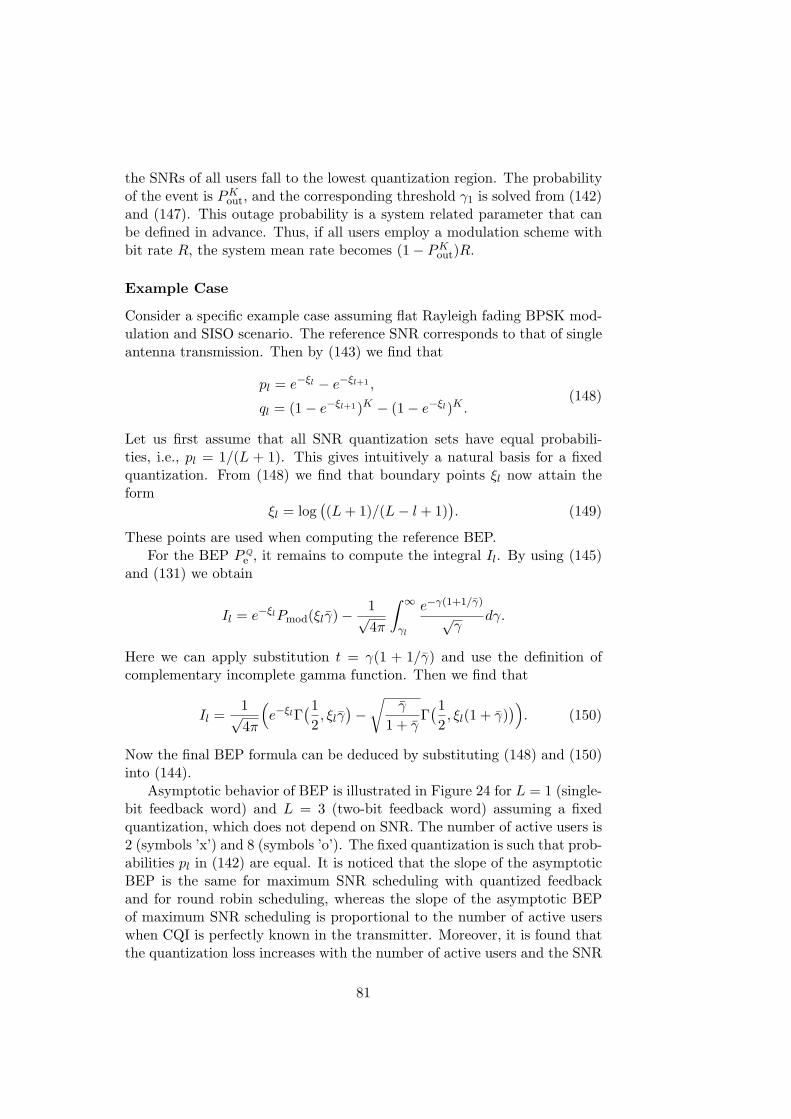
the SNRs of all users fall to the lowest quantization region. The probabilityof the event is PK

out, and the corresponding threshold γ1 is solved from (142)and (147). This outage probability is a system related parameter that canbe defined in advance. Thus, if all users employ a modulation scheme withbit rate R, the system mean rate becomes (1− PK

out)R.

Example Case

Consider a specific example case assuming flat Rayleigh fading BPSK mod-ulation and SISO scenario. The reference SNR corresponds to that of singleantenna transmission. Then by (143) we find that

pl = e−ξl − e−ξl+1 ,

ql = (1− e−ξl+1)K − (1− e−ξl)K .(148)

Let us first assume that all SNR quantization sets have equal probabili-ties, i.e., pl = 1/(L + 1). This gives intuitively a natural basis for a fixedquantization. From (148) we find that boundary points ξl now attain theform

ξl = log((L + 1)/(L− l + 1)

). (149)

These points are used when computing the reference BEP.For the BEP PQ

e , it remains to compute the integral Il. By using (145)and (131) we obtain

Il = e−ξlPmod(ξlγ)− 1√4π

∫ ∞

γl

e−γ(1+1/γ)

√γ

dγ.

Here we can apply substitution t = γ(1 + 1/γ) and use the definition ofcomplementary incomplete gamma function. Then we find that

Il =1√4π

(e−ξlΓ

(12, ξlγ

)−√

γ

1 + γΓ(12, ξl(1 + γ)

)). (150)

Now the final BEP formula can be deduced by substituting (148) and (150)into (144).

Asymptotic behavior of BEP is illustrated in Figure 24 for L = 1 (single-bit feedback word) and L = 3 (two-bit feedback word) assuming a fixedquantization, which does not depend on SNR. The number of active users is2 (symbols ’x’) and 8 (symbols ’o’). The fixed quantization is such that prob-abilities pl in (142) are equal. It is noticed that the slope of the asymptoticBEP is the same for maximum SNR scheduling with quantized feedbackand for round robin scheduling, whereas the slope of the asymptotic BEPof maximum SNR scheduling is proportional to the number of active userswhen CQI is perfectly known in the transmitter. Moreover, it is found thatthe quantization loss increases with the number of active users and the SNR

81

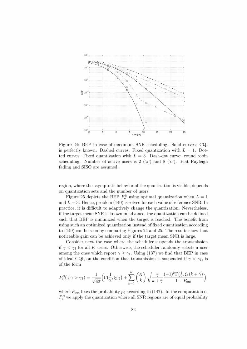
−10 −5 0 5 10 15 20 2510

−6

10−5

10−4

10−3

10−2

10−1

100

SNR [dB]

BE

P

Figure 24: BEP in case of maximum SNR scheduling. Solid curves: CQIis perfectly known. Dashed curves: Fixed quantization with L = 1. Dot-ted curves: Fixed quantization with L = 3. Dash-dot curve: round robinscheduling. Number of active users is 2 (’x’) and 8 (’o’). Flat Rayleighfading and SISO are assumed.

region, where the asymptotic behavior of the quantization is visible, dependson quantization sets and the number of users.

Figure 25 depicts the BEP P Qe using optimal quantization when L = 1

and L = 3. Hence, problem (140) is solved for each value of reference SNR. Inpractice, it is difficult to adaptively change the quantization. Nevertheless,if the target mean SNR is known in advance, the quantization can be definedsuch that BEP is minimized when the target is reached. The benefit fromusing such an optimized quantization instead of fixed quantization accordingto (149) can be seen by comparing Figures 24 and 25. The results show thatnoticeable gain can be achieved only if the target mean SNR is large.

Consider next the case where the scheduler suspends the transmissionif γ < γ1 for all K users. Otherwise, the scheduler randomly selects a useramong the ones which report γ ≥ γ1. Using (137) we find that BEP in caseof ideal CQI, on the condition that transmission is suspended if γ < γ1, isof the form

PQe (γ|γ > γ1) =

1√4π

(Γ(12, ξ1γ

)+

K∑

k=1

(Kk

) √γ

k + γ

(−1)kΓ(

12 , ξ1(k + γ

)

1− Pout

),

where Pout fixes the probability p0 according to (147). In the computation ofPQ

e we apply the quantization where all SNR regions are of equal probability

82

−10 −5 0 5 10 15 20 2510

−6

10−5

10−4

10−3

10−2

10−1

100

SNR [dB]

BE

P

Figure 25: BEP in case of maximum SNR scheduling. Solid curves: CQI isperfectly known. Dashed curves: Optimal quantization according to (140)with L = 1. Dotted curves: Optimal quantization according to (140) withL = 3. Dash-dot curve: round robin scheduling. Number of active users is2 (’x’) and 8 (’o’). Flat Rayleigh fading and SISO are assumed.

on the condition that γ > γ1. Thus, pl = (1 − p0)/L if l = 1, 2, . . . , L, andthe boundary points are given by

ξl = log(L/(1− p0)(L− l + 1)

). (151)

Figure 26 depicts the BEP curves for maximum SNR scheduling whenPout = 0.01, L = 1 and L = 3. Boundary points do not depend on SNR,and the number of active users is 2 (symbols ’x’) and 8 (symbols ’o’). Trans-mission is suspended also in case of perfect CQI, but in case of round robinscheduling transmission is continuous.

It is noticed that the quantization loss is already small in case of two-bit quantization even when the quantization is not optimized according toSNR. Furthermore, it is found that the asymptotic decay of all BEP curves,except the one corresponding to round robin scheduler, are exponential. Toconfirm this fact we recall (134) from Section 4.6 that shows the asymptoticBEP corresponding to single user SISO system, where the transmission issuspended if γ < γ1. Now we can apply the bound (146) where maximumand minimum is taken over indices l = 1, 2, . . . , L. Hence, the asymptoticdecay of the BEP is exponential also when feedback is quantized.

Transmit power control scheme, which achieves exponentially decayingBEP in MISO flat Rayleigh fading channels has also been reported in [81].

83

−10 −5 0 5 10 15 20 2510

−6

10−5

10−4

10−3

10−2

10−1

100

SNR [dB]

BE

P

Figure 26: BEP when maximum SNR scheduling is applied with 1% outageprobability. Solid curves: CQI is perfectly known. Dashed curves: fixedquantization with L = 1. Dotted curves: fixed quantization with L = 3.Dash-dot curve: round robin scheduling. Number of active users is 2 (’x’)and 8 (’o’). Flat Rayleigh fading and SISO are assumed.

The scheme assumes complete channel state information in the receiver inorder to achieve exponentially decaying BEP in every operation point, whilethe quantized feedback and suspension of transmission in Section 4.6 andin this section provide exponentially decaying BEP asymptotically in highSNR region.

The scheduler that suspends the transmission when SNRs of all usersfall below a threshold, provides asymptotically exponentially decaying BEPeven with suboptimal quantization. In fact, any reasonable quantizationstrategy provides this asymptotic performance as long as the system outageis allowed. This makes the system design much easier when compared tothe case, where quantization is optimized according to (140).

84

5 Scheduling for UTRA FDD Uplink

The importance of power control (PC) to the CDMA uplink performancehas motivated many studies such as [82], [83]. It is well-known that the meantransmit power in systems with PC depends on the channel fading statistics.The effect of the propagation environment is measured by power rise [84]that defines the ratio of the average transmit power in a fading channel tothat in a non-fading channel when the mean receive power is the same indifferent environments. Antenna diversity reduces channel variations andleads to a lower required transmit power as pointed out in [85], where powerrise was analyzed assuming flat fading.

In addition to antenna diversity also channel-aware scheduling will re-duce channel variations and thus, it reduces the required transmit powerin power controlled systems. Channel-aware scheduling can be beneficiallyused in uplink provided that base station scheduler can acquire CSI of dif-ferent users. This is possible in WCDMA uplink where control channelis continuously transmitted. Nevertheless, scheduling can be only appliedon the dedicated channel. Scheduling may increase the system efficiencythrough multi-user diversity if the total number of users in the system islarger than the number of transmitting users. However, since control chan-nels of waiting users are on, the control overhead increases with multi-userdiversity. Thus, the increased interference due to control signaling and de-creased interference due to scheduling should be considered jointly. Thisimportant problem seems to be widely ignored in the literature althoughthere are some research papers concerning uplink scheduling [86], [87], [88].

In this section, we study the effect of OOS to the required transmitpower [25]. In OOS we suspend the transmission if the channel power re-sponse falls below a predefined threshold. In practice this condition can beexplicitly verified from received power if PC is not applied and implicitlyfrom transmitted power if PC is on. In FDD WCDMA downlink, channelstate information can be obtained from the common omnidirectional pilotchannel that is transmitted with a fixed power. In WCDMA uplink, mobile’stransmit power on control channel varies according to channel fluctuationsand mobile can monitor its transmit power and suspend transmission ondata channel if a predefined power level is exceeded.

5.1 System Model

The basic idea of OOS in uplink is the same as it is in downlink. Hence, letγ0 denote a cutoff SNR and let γ be the instantaneous SNR. Then we definea relative threshold ξ = γ0/γ and suspend the transmission if γ/γ < ξ.Relative threshold is practical, because only the threshold crossings need tobe known in the transmitter and, on the other hand, the selection of TTI isfair if all users with the same service employ equal relative thresholds ξ.

85

In practical systems, γ needs to be estimated before OOS can be used.Moreover, receiver and transmitter have to agree on threshold values, butthis task can be carried out by employing long-term signaling on higher net-work layers. We note that in this work we do not fix specific threshold valuesbut show the effect of transmission probability, which is directly connectedto the threshold value, to the performance of OOS.

We assume a model where threshold crossings are known to the transmit-ter. Our generic communication protocol employs control channel (CCH)and data channel (DCH), and fast transmit power control is applied on bothchannels. A block multi-path Rayleigh fading model is adopted where thechannel remains constant during each TTI and channel coefficients betweenseparate TTIs are independent. Receiver has Mr antennas and it employsmaximal ratio combining over separate antennas and channel paths. Theexample radio channel models are ITU Pedestrian A and Pedestrian B pro-files [89], where relative mean path powers are 0.0 and -12.7 dB for the formerand 0.0, -0.9, -4.9, -8.0, -7.8 and -23.9 dB for the latter model. PedestrianB provides a realistic and challenging radio channel model for low mobilityenvironments, and it is applied in feasibility studies of uplink of UTRA FDDmode [70].

In the following we define three example systems that are analyzed. Werecall that all users connected to to base station need a CCH whether DCHis on or off.

System 1. There are Ktr users transmitting on DCH continuously. this caserepresents a circuit-switched system and possible services are, e.g., audio andvideo calls.

System 2. DCH transmission is not continuous but transmission times arerandomly selected from physical channel state point of view. The numberof transmitting users is Ktr while the total number of users in the system isK. This case represents a packet-switched system and possible services are,e.g., web browsing and FTP.

System 3. The system is similar to system 2, but now OOS is applied onDCH assuming error-free feedback channel.

System 2 represents a scheduler that does not take into account thestate of the physical channel, but transmission time intervals are selected,for example, based on delay requirements or buffer occupancy. The systemalso provides a good reference, because the use of channel state informationis the only difference between systems 2 and 3. Finally, we note that thetransmission probability of a user in systems 2 and 3 is defined by the numberof active users in the system, i.e., ptr = Ktr/K. Then cell throughput is thesame for all systems.

In Section 5.2 the transmit power gain from OOS is studied assuming

86

ideal power control, multi-path fading channel and Mr receive antennas.Since these assumptions are well valid in FDD WCDMA uplink we show inSection 5.3 how the OOS gain reflects to the coverage and capacity perfor-mance of FDD WCDMA.

The effect of transmission delay is neglected and we assume that dataservices are able to tolerate unbounded delays. This assumption is, of course,not realistic, but instead of designing a practical scheduling algorithm ouraim is to study, how the control signaling overhead may limit the perfor-mance of physical layer scheduling. On-off scheduling is compared to tworeference systems.

5.2 Analysis of Transmit Power

Due to PC, the target received power in the base station remains approxi-mately the same although the link performance is improved. Furthermore,OOS reduces mobile’s mean transmit power, because transmission is sus-pended during the deep fades. Assuming ideal power control in the sensethat the received power remains constant all the time, we have

Pk,dγ = Prx,d, Pcγ = Prx,c

where Prx,d and Prx,c are the target received powers for data and controlchannels, respectively, γ is the power response of the physical channel, andPk,d and Pc refer to the instantaneous transmit powers of a user of kthexample system on data and control channels respectively. The transmitpower of the control channel is assumed to be the same in all systems. Thiskind of power control essentially inverts the channel and better power controlstrategies are available [81]. Fast PC in WCDMA approximates the channelinverse, and it has been shown that different MIMO solutions in WCDMAuplink can be analyzed based on the ideal power control assumption [26], [27]and the results closely match to link-level simulations.

In the following the relative link level performance between the threeexample systems is measured by using the ratio between expected transmitpowers. While comparing systems 2 and 3 we use the ratio

ρ2,3 =Ktr · P2,d + K · Pc

Ktr · P3,d + K · Pc=

ptrP2,d + Pc

ptrP3,d + Pc, (152)

where P2,d, P3,d, Pc refer to the corresponding mean transmit powers. Werecall that OOS is applied only on the data channel in System 3. Hence, wecan write

P3,d = EPd|γ > γ0, P2,d = P1,d = EPd =: Pd.

In the following we employ notations

ρ0 =Pd

P3,d, R =

Pc

Pd· ptr, (153)

87

Data rate on DCH [kbps] 12.2 64 144 384 2048Power ratio CCH/DCH [dB] -2.69 -5.46 -9.54 -9.54 -9.54

Table 6: Recommended power ratios between CCH and DCH in FDDWCDMA uplink.

where ρ0 is the relative power rise that indicates the gain of OOS on the datachannel. Moreover, R defines the ratio of mean transmit powers betweencontrol and data channels. In general the value of R can be optimized foreach service. However, it is easier to apply fixed values that are definedin advance. For FDD WCDMA such values, presented in Table 6, wereproposed in [90]. Furthermore, the effect of power offset between enhanceddata and control channels was studied in [70].

Mean transmit power of the control channel Pc is scaled by the transmis-sion probability to keep the ratio between powers of DCH and CCH the samefor all systems although systems 2 and 3 apply discontinuous transmission.After combining (152) and (153) we obtain

ρ2,3 =ρ0(p2

tr + R)p2

tr + ρ0R. (154)

It is worth noticing that ρ2,3 → 1 if ptr → 0 or ptr → 1. The former limitfollows, because the gain of system 3 against system 2 vanishes when thetransmission probability is small and control channel overhead of the userswaiting in the queue becomes dominating. On the other hand, the gainalso vanishes if ptr → 1, because transmission in systems 2 and 3 becomescontinuous. We also note that ρ2,3 = ρ0 if control channel does not exist.

While the ratio R is defined by the service, ρ0 attains a closed-formexpression in case of Rayleigh fading environment. Before considering thistopic we deduce ratios ρ1,3 and ρ1,2. We have

ρ1,3 =Ktr(Pd + Pc)

Ktr · P3,d + K · Pc= ρ0 · ptr

ptr + R

p2tr + ρ0R

. (155)

Finally, combining (154) and (155) we obtain

ρ1,2 = ptr · ptr + R

p2tr + R

.

At this stage we focus on ρ0. The computation of power rise was pre-viously considered in [85], but the analysis therein covers only continuoustransmission (γ0 = 0) assuming a single path channel, while our aim is tocompute ρ0 for OOS and PC within multi-path environment. We have

P3,d = Prx,d

∫ ∞

γ0

f(γ)/γdγ, (156)

88

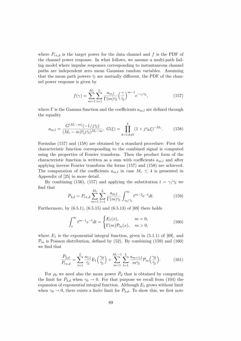
where Prx,d is the target power for the data channel and f is the PDF ofthe channel power response. In what follows, we assume a multi-path fad-ing model where impulse responses corresponding to instantaneous channelpaths are independent zero mean Gaussian random variables. Assumingthat the mean path powers γl are mutually different, the PDF of the chan-nel power response is given by

f(γ) =Mr∑

m=1

L∑

l=1

am,l

Γ(m)γl

( γ

γl

)m−1e−γ/γl , (157)

where Γ is the Gamma function and the coefficients am,l are defined throughthe equality

am,l =G(Mr−m)(−1/jγl)

(Mr −m)!(jγl)Mr−m, G(ξ) =

L∏

k=1,k 6=l

(1 + jγkξ)−Mr . (158)

Formulas (157) and (158) are obtained by a standard procedure: First thecharacteristic function corresponding to the combined signal is computedusing the properties of Fourier transform. Then the product form of thecharacteristic function is written as a sum with coefficients am,l and afterapplying inverse Fourier transform the forms (157) and (158) are achieved.The computation of the coefficients am,l in case Mr ≤ 4 is presented inAppendix of [25] in more detail.

By combining (156), (157) and applying the substitution t = γ/γl wefind that

P3,d = Prx,d

Mr∑

m=1

L∑

l=1

am,l

Γ(m)γl

∫ ∞

γ0/γl

tm−2e−tdt. (159)

Furthermore, by (6.5.1), (6.5.15) and (6.5.13) of [69] there holds

∫ ∞

xtm−1e−tdt =

E1(x), m = 0,

Γ(m)Pm(x), m > 0,(160)

where E1 is the exponential integral function, given in (5.1.1) of [69], andPm is Poisson distribution, defined by (52). By combining (159) and (160)we find that

P3,d

Prx,d=

L∑

l=1

a1,l

γlE1

(γ0

γl

)+

Mr−1∑

m=1

L∑

l=1

am+1,l

mγlPm

(γ0

γl

). (161)

For ρ0 we need also the mean power Pd that is obtained by computingthe limit for P3,d when γ0 → 0. For that purpose we recall from (104) theexpansion of exponential integral function. Although E1 grows without limitwhen γ0 → 0, there exists a finite limit for P3,d. To show this, we first note

89

that f(0) = 0 if Mr ·L > 1. This holds because f is a convolution of Mr ·Lchi-square distributions. Then we find by (157) that

L∑

l=1

a1,l

γl= 0. (162)

Let us denote E1(x) + log(x) = g(x). Then, by employing (162) we canwrite for any γ0 > 0

L∑

l=1

a1,l

γlE1

(γ0

γl

)=

L∑

l=1

a1,l

γl

(E1

(γ0

γl

)+ log

(γ0

γ

))

= −L∑

l=1

a1,l

γl

(log

( γ

γl

)− g

(γ0

γl

)).

By applying equations g(0) = −e0 and (162) we find that

limγ0→0

L∑

l=1

a1,l

γlE1

(γ0

γl

)= −

L∑

l=1

a1,l

γllog

( 1σ2

l

), (163)

where σ2l = γl/γ refers to the normalized mean path powers. Finally, by

using the fact that Pm(0) = 1, and equation (163), we obtain

Pd

Prx,d= −

L∑

l=1

a1,l

γllog

( γ

γl

)+

Mr−1∑

m=1

L∑

l=1

am+1,l

mγl. (164)

The expression for ρ0 is obtained by combining (161) and (164). Applyingnotation ξ = γ0/γ we get

ρ0 =−

L∑l=1

a1,l

σ2l

log(

1σ2

l

)+

Mr−1∑m=1

L∑l=1

am+1,l

mσ2l

L∑l=1

a1,l

σ2l

E1

( ξσ2

l

)+

Mr−1∑m=1

L∑l=1

am+1,l

mσ2lPm

( ξσ2

l

) . (165)

The parameter ξ in (165) reflects the effect of the transmission threshold andit can be solved for a given transmission probability ptr from the equation

ptr =∫ ∞

γ0

f(γ)dγ =Mr∑

m=1

L∑

l=1

am,lPm(ξ) (166)

that is obtained by employing the substitution t = γ/γl and expression (160).Solution for (166) is found numerically by applying, for example, the bisec-tion method, and the solution is unique because P (γ > γ0) is a monotonic

90

function with respect to γ0. After solving ξ, the relative power rise ρ0 iscomputed by using (165).

Before closing this section we shortly consider two important issues.Firstly, for a fixed ratio R there exists a probability ptr such that

ρ2,3 = max0≤ptr≤1

(ρ2,3) =ρ0(p2

tr + R)p2

tr + ρ0R,

where ρ0 = ρ0(ptr). We will further illustrate this topic in Section 5.4. Sec-ondly, many practical services are delay sensitive and therefore low trans-mission probabilities are not favorable. A lower bound to the transmissiondelay is obtained by assuming a memoryless channel such that channel statesof consecutive transmission time intervals are independent. Then the proba-bility that the delay exceeds t transmission time intervals is (1−ptr)t, whichdecays rapidly unless ptr is small. However, if a user is moving with a lowspeed, such that the channel states between consecutive transmission timeintervals are highly correlated, the delays can become intolerably long. Ourmodel is rather coarse and a more detailed system model would be neededto carry out a detailed study on delay issues.

5.3 OOS Gain in WCDMA Uplink

Since PC drives the received power to the target value corresponding to theselected service, scheduling gain is seen in the terminal as a decrease in therequired transmission power. This gain further effects the system coverageand capacity via the following three mechanisms:

• In isolated cell the decrease in required transmit power in mobile stationreflects directly to the cell coverage and service availability.• If scheduling is applied in the whole network, lower transmit power will alsodecrease the inter-cell interference. This reflects to increased cell capacityin interference limited cells.• If system supports adaptive coding and modulation, mobile can increasethe link throughput in good channel conditions.

We study in more detail the first two gain mechanisms that can berealized in WCDMA uplink. The third gain mechanism is not applicable inWCDMA uplink because the present specification does not support adaptivemodulation and coding in uplink.

Let us consider first the coverage. For that purpose we recall the mostwidely used Okumura-Hata propagation model model [91, 92] that is validin macro-cell environments where base station antennas are placed abovethe rooftop level. The usual operating frequency of WCDMA uplink is 1950MHz and the corresponding path loss in decibels in Okumura-Hata modelis given by

Lp = 157.83− 13.82 log10(HBS)−A(HMS) +(B − 6.55 log10(HBS)

)log10(D),

91

Service [kbps] 12.2 64 144 384Allowed Lp [dB] 140.20 136.86 136.02 132.26Max. Range [km] 1.12 0.90 0.85 0.67

Table 7: Allowed propagation losses and cell ranges for some service classesin FDD WCDMA uplink.

where D is the distance (km) between base and mobile stations, HBS (m)is the base station antenna height, HMS (m) is the mobile station antennaheight, B is a user-defined parameter whose value is commonly set to 44.9,and for large city A is defined by

A(HMS) = 3.2(log10(11.75HMS)

)2 − 4.97.

We follow [93] where base station and mobile station antenna heights inurban macro-cell are 25 m and 1.5 m, respectively. Then

Lp = 138.5 + 35.7 log10(D). (167)

Maximum allowed path loss in WCDMA is estimated by radio link budget(RLB) calculation. The RLB contains round 20 parameters and we referto [93] and [37] for more details. In Table 7 we have recalled from [93],p.121 the allowed propagation loss figures for some services.

The allowed propagation losses in Table 7 are not directly proportionalto the data rate because the assumptions, such as coverage probability, aredifferent for different services. The maximum cell ranges for different servicescan be computed from (167), and the coverage gain of OOS is obtained bycomparing the required transmit powers in systems 2 and 3.

Assume that the allowed path loss figures of Table 7 are valid for system2 with Mr = 1. If we replace system 2 by system 3 with OOS, the gainin mobile station transmission power is obtained according to ρ2,3 and thecorresponding value can be added to the RLB. Then cell ranges D2 and D3

for systems 2 and 3 can be calculated from (167) and the correspondingcoverage gain is (D2

3 −D22)/D2

2. If Mr > 1, the allowed propagation loss forboth systems increases roughly by log10(Mr).

We would have been able to compute the relative gain from OOS directlyfrom (167). However, by utilizing the link budget examples we are able tocompute example ranges showing also an estimate of the absolute gainsof OOS. Finally, we note that RLB calculations rely on several variables,some of them being rather uncertain. Therefore, the absolute range figuresrepresent only rough approximations. We will show coverage gain figures inSection 5.4.

92

Capacity gains are analyzed by using noise rise, denoted by µ, which isdefined as a ratio of the total received wideband power to the thermal noisepower [37]. Noise rise is a function of system load η,

µ =1

1− η. (168)

The more loading is allowed in the system, the larger is the required interfer-ence margin µ0 = maxµ and the smaller is the coverage area. Interferencemargin defines the maximum allowed noise rise and values up to 6 dB areused [37]. The formula for system load is of the form

η = (1 + ν)Nown∑

n=1

κnErx,n

1 + κnErx,n, (169)

where ν = Iother/Iown is the inter-cell to intra-cell interference ratio seen bythe base station receiver, Nown is the number of own cell users, κn is theratio between the bit rate and chip rate, and Erx,n is the received energyper data bit divided by the noise spectral density (Eb/N0) of nth user, seeSection 6 and [37].

Assume that the number of receive antennas is fixed. OOS reduces themobile’s transmit power but it does not reduce the received Eb/N0, becausepower control maintains the received power at the target level defined bythe required QoS. Therefore, OOS does not improve capacity in isolated cellwhere ν = 0 and inter-cell interference does not exist. However, OOS de-creases the inter-cell interference in interference limited cases where ν > 0.Let us consider the effect in more detail: According to (168), the theoreticalcapacity limit is reached when load approaches the 100% level and the corre-sponding maximum number of users is obtained from (169). Assuming thatall users employ the same service we may denote κn =: κ, Erx,n =: Erx andthe computation of the cell throughput is straightforward. Suppose that thenumber of receive antennas and the number of users are fixed in systems 2and 3. By (169) we obtain

η3

η2=

Erx,3(1 + κ · Erx,2)Erx,2(1 + κ · Erx,3)

· 1 + ν3

1 + ν2=

1 + ν3

1 + ν2, (170)

where numbers 2 and 3 refer to different systems and the latter equalityfollows because the target Eb/N0 remains constant. Inter-cell interferenceratio ν3 can be written as

ν3 =ν3

ν2· ν2 =

Iother,3

Iother,2· ν2. (171)

Hence, it remains to study the inter-cell interference. There holds

Iother,k =Nother∑

n=1

EQn,kγn =Nother∑

n=1

Qn,kγn, (172)

93

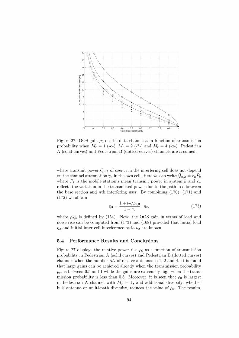
0 0.1 0.2 0.3 0.4 0.5 0.6 0.7 0.8 0.9 10

2

4

6

8

10

12

14

16

18

20

OO

S G

ain

on d

ata

chan

nel [

dB]

Transmission probability

Figure 27: OOS gain ρ0 on the data channel as a function of transmissionprobability when Mr = 1 (-o-), Mr = 2 (-*-) and Mr = 4 (-x-). PedestrianA (solid curves) and Pedestrian B (dotted curves) channels are assumed.

where transmit power Qn,k of user n in the interfering cell does not dependon the channel attenuation γn in the own cell. Here we can write Qn,k = cnPk

where Pk is the mobile station’s mean transmit power in system k and cn

reflects the variation in the transmitted power due to the path loss betweenthe base station and nth interfering user. By combining (170), (171) and(172) we obtain

η3 =1 + ν2/ρ2,3

1 + ν2· η2, (173)

where ρ2,3 is defined by (154). Now, the OOS gain in terms of load andnoise rise can be computed from (173) and (168) provided that initial loadη2 and initial inter-cell interference ratio ν2 are known.

5.4 Performance Results and Conclusions

Figure 27 displays the relative power rise ρ0 as a function of transmissionprobability in Pedestrian A (solid curves) and Pedestrian B (dotted curves)channels when the number Mr of receive antennas is 1, 2 and 4. It is foundthat large gains can be achieved already when the transmission probabilityptr is between 0.5 and 1 while the gains are extremely high when the trans-mission probability is less than 0.5. Moreover, it is seen that ρ0 is largestin Pedestrian A channel with Mr = 1, and additional diversity, whetherit is antenna or multi-path diversity, reduces the value of ρ0. The results,

94

0 0.1 0.2 0.3 0.4 0.5 0.6 0.7 0.8 0.9 1−3

−2

−1

0

1

2

3

4

5

Rat

io b

etw

een

expe

cted

tran

smit

pow

ers

[dB

]

Transmission probability

Figure 28: Ratio ρ13 (dashed curves) and ρ23 (dotted curves) as a functionof transmission probability when Mr = 1 (-o-), Mr = 2 (-*-) and R = −9.54dB. Pedestrian A channel is assumed. Ratio ρ12 between systems 1 and 2 isdepicted by a solid curve.

however, do not directly define the performance of system 3 against systems1 and 2 because the effect of control channel overhead is not taken intoaccount.

Figures 28 and 29 show the relative transmit powers ρ12, ρ13 and ρ23

in Pedestrian A and B channels as a function of transmit probability whenthe number of receive antennas is 1 and 2, and the power ratio betweencontrol and data channels is −9.54 dB (adopted from Table 6). Since OOSis not applied on the control channel, the gain of system 3 against systems1 and 2 vanishes when the transmission probability is small and controlchannel overhead of the waiting users becomes dominating. On the otherhand, the gain also vanishes if ptr → 1, because transmission in systems 2and 3 becomes continuous. As noticed before, there exists a transmissionprobability that maximizes the relative gain of system 3 against systems 1and 2. The probability giving the maximum gain depends on the channelprofile, Mr and the ratio R while the magnitude of the maximum gain mainlydepends on R. Before further studying this subject we note that accordingto Figures 28 and 29, the performance of system 2 is inferior to system 1 asone can expect, because control channel overhead is smaller in system 1.

Figure 30 depicts the maximum gain of system 3 against system 2 as afunction of R. As expected, the OOS gain is large when R is small showingthat the best OOS gains are obtained when transmit power on data channel

95

0 0.1 0.2 0.3 0.4 0.5 0.6 0.7 0.8 0.9 1−3

−2

−1

0

1

2

3

4

5

Rat

io b

etw

een

expe

cted

tran

smit

pow

ers

[dB

]

Transmission probability

Figure 29: Ratio ρ13 (dashed curves) and ρ23 (dotted curves) as a function oftransmission probability when Mr = 1 (-o-) and Mr = 2 (-*-) and R = −9.54dB. Pedestrian B channel is assumed. Ratio ρ12 between systems 1 and 2 isdepicted by a solid curve.

is large when compared to control channel power. This is usually the casefor high data rates.

Figure 31 displays the transmission probabilities corresponding to thelargest gains ρ2,3 as a function of R. It is found that the transmission prob-ability ptr giving the best performance is increasing with R. However, inpractice users’ data rates and the number of users cannot be very large simul-taneously, because the cell capacity is limited. Therefore, small transmissionprobabilities are usually not feasible in practice.

Let us now recall the RLB example of Table 7. Table 8 lists maximumcell ranges for 384 kbps service in systems 2 and 3 assuming PedestrianA and Pedestrian B channels and one and two receive antennas. Rangesare computed using (167) and the allowed path loss according to Table 7.System 2 with Mr = 1 serves as the reference and maximum OOS gain ρ2,3

is applied.It is found that relative coverage gains are large. However, when services

have different ratios R the gains would be smaller, because there is no op-timal transmission probability for all services. Moreover, the analysis doesnot take into account practical unidealities like threshold estimation andfeedback errors. Yet, it can be expected that OOS remarkably improves theavailability of medium and high data rate services.

Finally, Figure 32 illustrates the decrease in system load when applying

96

−20 −18 −16 −14 −12 −10 −8 −6 −4 −2 00

1

2

3

4

5

6

7

8

9T

rans

mit

pow

er r

atio

bet

wee

n sy

stem

s 2

and

3 [d

B]

Ratio between control and data channel powers [dB]

Figure 30: Ratio ρ23 as a function of R when Mr = 1 (-o-), Mr = 2 (-*-)and Mr = 4 (-x-). Pedestrian A (solid curves) and Pedestrian B (dashedcurves) channels are assumed.

−20 −18 −16 −14 −12 −10 −8 −6 −4 −2 00.2

0.3

0.4

0.5

0.6

0.7

0.8

Tra

nsm

issi

on P

roba

bilit

y

Ratio between control and data channel powers [dB]

Figure 31: Transmission probability ptr as a function of R when Mr = 1(-o-), Mr = 2 (-*-) and Mr = 4 (-x-). Pedestrian A (solid curves) andPedestrian B (dashed curves) channels are assumed.

97

Channel Setup D, system 2 [km] D, system 3 [km] Coverage gainPed. A, Mr = 1 0.67 0.89 76%Ped. A, Mr = 2 0.81 1.01 55%Ped. B, Mr = 1 0.67 0.81 46%Ped. B, Mr = 2 0.81 0.96 40%

Table 8: Cell ranges for 384 kbps service when Pedestrian A and B areassumed and Mr = 1, 2.

0 0.2 0.4 0.6 0.8 1 1.2 1.4 1.6 1.8 20

5

10

15

20

25

30

35

40

Initial intercell interference ratio

Dec

reas

e in

load

due

to O

OS

[%]

Figure 32: Decrease in FDD WCDMA uplink load due to OOS as a func-tion of inter-cell interference ratio ν2 when R = −9.54 dB and η2 = 0.75.Channels are Pedestrian A (solid curves) and Pedestrian B (dotted curves),and number of receive antennas are Mr = 1 (-o-) and Mr = 2 (-*-).

98

OOS. The curves are deduced from equation (173) by assuming η2 = 0.75and employing ratio (154) with R = −9.54 dB. It is seen that the load ofsystem 3 is remarkably smaller than that of system 2. Nevertheless, the gainstrongly depends on the initial inter-cell interference ratio ν2. For example,for omnidirectional base station antennas ν2 = 0.55 [37]. Moreover, OOSgains are smaller when initial load η2 is small.

99

6 MIMO in UTRA FDD Uplink

The introduction of MIMO [94], [95], [96] has fueled several research papers,see [97]. Most of the studies assume broadcast channel and are applicablein cellular downlink but there are also some works that consider MIMO inCDMA uplink [98], [99] that is our focus in this section.

Similarly with the main stream research, in 3GPP the MIMO discussionhas focused on downlink [100]. Nevertheless, the introduction of new servicessuch as videophones will make it extremely important to reach high spectralefficiency also in the uplink direction. Besides this service based demand,there are also two evident reasons why MIMO in UTRA FDD uplink isattractive and thus, worth of a closer study. Firstly, base stations will havetwo or more antennas in the near future, and at the same time two-antennamobiles, which are at least capable of interference cancellation, will becomemore common. Secondly, in contrast with UTRA FDD downlink, only minorchanges to the UTRA FDD specifications are needed to enable simple uplinkMIMO approaches. The content of this section is based on [26], [27] and [28].

6.1 MIMO Algorithms

We divide MIMO techniques into two main classes, namely to diversity andinformation MIMO. UTRA FDD uplink provides good means to implementdiversity and information MIMO techniques, because uplink users are sepa-rated by different scrambling codes and therefore the whole channelizationcode space is available for any one user.

Diversity MIMO

In diversity MIMO, Mt replicas of the same data stream are transmittedby using different orthogonal channelization codes but the same scramblingcode. This is depicted in Figure 33 which shows the system model of di-versity MIMO for two transmit antennas. The received signal in kth basestation antenna becomes

yk(t) =∞∑

i=−∞

Mt∑

m=1

hm,k(t) ∗√

Ptx

Mt

Sd,m(t) + j · Sc,m(t)

,

Sx,m(t) = bx[i] · βx · cx,m(t− iTx − δ)⊗ sdpch(t− iTs − δ),

(174)

where x ∈ d, c, ∗ refers to convolution with multi-path channel hm,k,and ⊗ refers to chip-by-chip multiplication of user’s scrambling code sdpch

and channelization codes cd,m and cc,m of dedicated physical data channel(DPDCH) and dedicated physical control channel (DPCCH), respectively.Total transmit power is given by Ptx and power ratio between DPDCH andDPCCH is adjusted by scaling factors βd and βc, and user’s transmitted

100

Figure 33: System model for diversity MIMO.

bits in DPDCH and DPCCH are denoted by bd and bc. Users are notsynchronized in uplink, and the delay is denoted by δ. Finally Td, Tc, andTs refer to the lengths of the two channelization codes and the scramblingcode.

Each transmit antenna uses different channelization codes cd,m and cc,m

so that the base stations can separate the signals from different antennasand later combine them using maximal ratio combining. Thus, the schemedoubles the usage of uplink channelization codes when compared to singleantenna transmission. The achievable bit rate with diversity MIMO is atmaximum 2 Mbps/Mt. This reduction of maximum bit rate could be partlyavoided by puncturing the applied error correcting codes, but informationMIMO provides a more attractive choice because the reduced code rate quiterapidly destroys system performance. However, for low and medium bit rateservices this does not present a problem.

We note that in case of flat fading and perfect CSI in the receiver, thelink performance of the proposed two-antenna diversity MIMO algorithmis the same as with STTD, because the diversity order of both schemes istwo. However, the system utilizing orthogonal channelization codes is morerobust, because orthogonality of the received signals does not depend on thechannel estimation as in the case of space-time coding.

Information MIMO

In case of information MIMO of Figure 34, a composite data stream ismultiplexed into two or more independent substreams that are transmittedfrom separate antennas by employing different scrambling codes. All streamscontain DPDCH and DPCCH so that in base station they can be interpretedas signals from different independent users. The received wideband signal

101

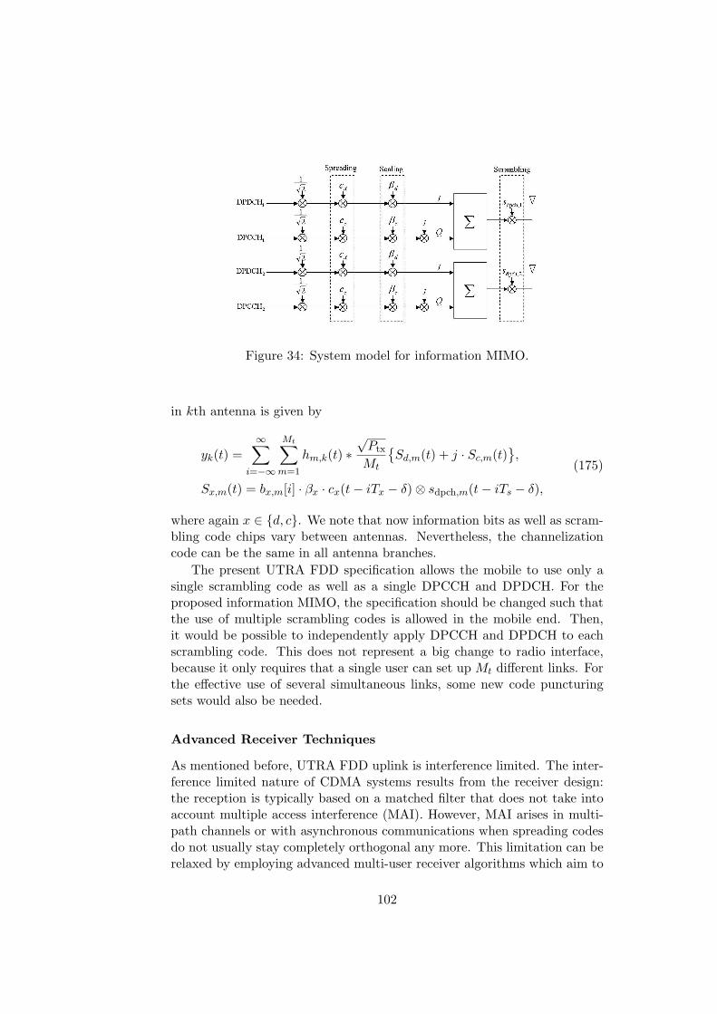
Figure 34: System model for information MIMO.

in kth antenna is given by

yk(t) =∞∑

i=−∞

Mt∑

m=1

hm,k(t) ∗√

Ptx

Mt

Sd,m(t) + j · Sc,m(t)

,

Sx,m(t) = bx,m[i] · βx · cx(t− iTx − δ)⊗ sdpch,m(t− iTs − δ),

(175)

where again x ∈ d, c. We note that now information bits as well as scram-bling code chips vary between antennas. Nevertheless, the channelizationcode can be the same in all antenna branches.

The present UTRA FDD specification allows the mobile to use only asingle scrambling code as well as a single DPCCH and DPDCH. For theproposed information MIMO, the specification should be changed such thatthe use of multiple scrambling codes is allowed in the mobile end. Then,it would be possible to independently apply DPCCH and DPDCH to eachscrambling code. This does not represent a big change to radio interface,because it only requires that a single user can set up Mt different links. Forthe effective use of several simultaneous links, some new code puncturingsets would also be needed.

Advanced Receiver Techniques

As mentioned before, UTRA FDD uplink is interference limited. The inter-ference limited nature of CDMA systems results from the receiver design:the reception is typically based on a matched filter that does not take intoaccount multiple access interference (MAI). However, MAI arises in multi-path channels or with asynchronous communications when spreading codesdo not usually stay completely orthogonal any more. This limitation can berelaxed by employing advanced multi-user receiver algorithms which aim to

102

reduce MAI. Information MIMO increases MAI in base station, and there-fore advanced receivers become important to the system performance whenimplementing information MIMO techniques.

In order to avoid the overwhelming complexity of multi-user detectionvarious sub-optimal multi-user receivers have been developed to cope withMAI. The multi-user receivers can be categorized in several ways. One pos-sibility is to classify the receivers to linear (decorrelating detector, minimummean square error (MMSE) detector) and non-linear receivers. Subtractiveinterference cancellation (IC) is one example of the latter category whichfirst estimates the MAI component and then subtracts it from the receivedsignal to improve the reliability of the symbol decisions.

Cancellation of MAI can be carried out in parallel to all users, i.e. withparallel interference cancellation (PIC) receivers, or in a serial fashion, i.e.using serial interference cancellation (SIC) receivers. In un-decoded (con-ventional) PIC receivers, IC is based on tentative symbol decisions. Thequality of the tentative decisions is essential, because incorrect decisions in-crease interference instead of decreasing it. In practice, the error rate ofun-decoded bits varies between 5% and 20% in UTRA FDD uplink. The er-ror rate depends mainly on the effective coding rate (i.e., rate of the channelencoder taking into account possible repetition and puncturing), the radioenvironment and the quality of service requirements.

Unreliable tentative bit decisions compromise the performance of un-decoded PIC. One possibility to improve the reliability of the decisions is tofirst decode the received symbols, re-encode the decoded symbols again, andfinally subtract the contribution of the re-encoded symbols from the receivedsignal. For more details we refer to [101] where this kind of decoded PIC isapplied to the convolutionally coded CDMA system. In [102], this idea isextended to Turbo coded CDMA system.

6.2 Uplink Load Equations

Load equations provide a useful tool in both initial planning and per-formance analysis of the network. Here we represent the load equa-tions [37], [93] that will serve as a basis for further studies.

Basic Load Equations

In the following Nown and Nother refer to the number of own cell and othercell users, respectively. The received wideband signal in baseband at timeinstant t can be expressed in the form

r(t) =Nown∑

n=1

yn(t) +Nother∑

n=1

zn(t) + n(t), (176)

103

where n(t) is complex zero-mean Gaussian, yn(t) is the interference fromnth own cell user and zn(t) is the interference from nth other cell user. Thesystem load can be estimated from the sum of received wideband powers ofdifferent users. Signals from different users are mutually independent andfrom (176) the received wideband power is given by

E|r(t)|2 = Itotal = Iown + Iother + PN,

where PN is the noise power and

Iown =Nown∑

n=1

E|yn(t)|2, Iother =Nother∑

n=1

E|zn(t)|2.

Received energy per data bit divided by the noise spectral density is animportant variable in the analysis of UTRA FDD uplink. For user n it isgiven by

Erx,n =1κn

· Prx,n

Itotal − Prx,n, (177)

where Prx,n refers to the received power, and κn is the ratio between bit rateand chip rate of user n. In UTRA FDD uplink, fast power control tries tokeep Erx,n at a target level. Therefore, changes in the interference do notreflect to Erx,n as long as power control is able to compensate the increasedinterference through Prx,n. From (177) we easily find that

Prx,n =κnErx,n

1 + κnErx,n· Itotal =: ηn · Itotal,

where ηn is the load from nth user. For the received wideband power in theown cell there holds

Iown =Nown∑

n=1

Prx,n =Nown∑

n=1

ηn · Itotal. (178)

Furthermore, the total wideband power can be written in the form

Itotal = Iown + Iother + PN =(1 + ν)Iown + PN, (179)

where ν = Iother/Iown is the inter-cell to intra-cell interference ratio seen bythe base station receiver. After combining (178) and (179) and solving Itotal

from the resulting formula we obtain the following expression for the noiserise

µ =Itotal

PN

=(1− (1 + ν)

Nown∑

n=1

ηn

)−1,

where the sum term defines the own cell load η. In UTRA FDD uplink,load control drives noise rise to a target level. The more loading is allowed

104

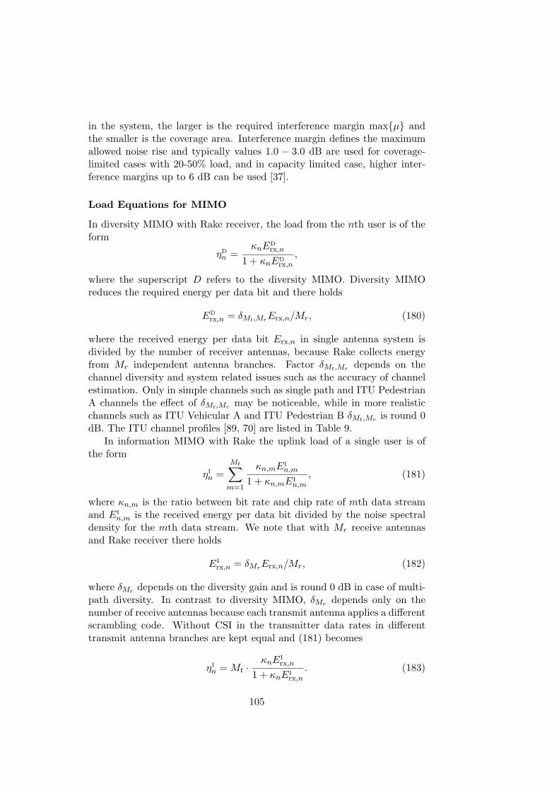
in the system, the larger is the required interference margin maxµ andthe smaller is the coverage area. Interference margin defines the maximumallowed noise rise and typically values 1.0 − 3.0 dB are used for coverage-limited cases with 20-50% load, and in capacity limited case, higher inter-ference margins up to 6 dB can be used [37].

Load Equations for MIMO

In diversity MIMO with Rake receiver, the load from the nth user is of theform

ηDn =

κnEDrx,n

1 + κnEDrx,n

,

where the superscript D refers to the diversity MIMO. Diversity MIMOreduces the required energy per data bit and there holds

EDrx,n = δMt,MrErx,n/Mr, (180)

where the received energy per data bit Erx,n in single antenna system isdivided by the number of receiver antennas, because Rake collects energyfrom Mr independent antenna branches. Factor δMt,Mr depends on thechannel diversity and system related issues such as the accuracy of channelestimation. Only in simple channels such as single path and ITU PedestrianA channels the effect of δMt,Mr may be noticeable, while in more realisticchannels such as ITU Vehicular A and ITU Pedestrian B δMt,Mr is round 0dB. The ITU channel profiles [89, 70] are listed in Table 9.

In information MIMO with Rake the uplink load of a single user is ofthe form

ηIn =

Mt∑

m=1

κn,mEIn,m

1 + κn,mEIn,m

, (181)

where κn,m is the ratio between bit rate and chip rate of mth data streamand EI

n,m is the received energy per data bit divided by the noise spectraldensity for the mth data stream. We note that with Mr receive antennasand Rake receiver there holds

EIrx,n = δMrErx,n/Mr, (182)

where δMr depends on the diversity gain and is round 0 dB in case of multi-path diversity. In contrast to diversity MIMO, δMr depends only on thenumber of receive antennas because each transmit antenna applies a differentscrambling code. Without CSI in the transmitter data rates in differenttransmit antenna branches are kept equal and (181) becomes

ηIn = Mt ·

κnEIrx,n

1 + κnEIrx,n

. (183)

105

Equation (183) indicates that base station receiver sees the usage ofinformation MIMO as an increased number of SISO users. This additionalload can be effectively reduced by applying PIC, which removes part ofthe own cell interference in the detection process. Let us denote the PICefficiency by β, 0 ≤ β ≤ 1. Then the average load of a single user can bewritten as

ηn = (1− β)κnErx,n

1 + κnErx,n.

Since PIC is not able to remove the inter-cell interference the total widebandpower seen by base station receiver is of the form

Itotal = (1− β)Iown + Iother + PN = (1− β + ν)Iown + PN

and the corresponding cell load is given by

η = (1− β + ν)Nown∑

n=1

ηn. (184)

In case of PIC diversity MIMO operates in a similar manner as in case ofSISO. For a single user load we have

ηDn = (1− β)

κnEDrx,n

1 + κnEDrx,n

. (185)

Furthermore, for information MIMO the single user load is given by

ηIn = (1− β)

Mt∑

m=1

κn,mEIrx,n,m

1 + κn,mEIrx,n,m

. (186)

6.3 Performance Comparisons

In the following we show performance results for UTRA FDD uplink anddiscuss the connection between the results and the load equations. Simu-lations use full 3GPP link level modeling with inner and outer loop powercontrol and realistic channel and interference estimation algorithms. Theradio channel is modeled according to ITU models in Table 9. Our sys-tem model follows accurately the present UTRA FDD specifications andsimulations are done following strictly the recommendations given in [89].

Let us consider two systems where the number of users is the same and allusers employ the same service. Assume that the number of receive antennasis the same in both systems but the first system applies the diversity MIMOwhile the second one employs single-input multiple-output (SIMO). In bothsystems, base station applies Rake receiver. Then, according to (180) theratio between cell loads is given by

ηsys2

ηsys1

=δ1,MrErx/Mr(1 + κ · δMt,MrErx/Mr)δMt,MrErx/Mr(1 + κ · δ1,MrErx/Mr)

· 1 + ν2

1 + ν1,

106

Model delay profile [ns] power profile [dB]Ped. A 0, 110, 190, 410, 0, −9.7, −19.2, −22.8Ped. B 0, 200, 800, 1200, 2300, 3700 0, −0.9, −4.9, −8.0, −7.8, −23.9Veh. A 0, 310, 710, 1090, 1730, 2510 0, −1, −9, −10, −15, −20

Table 9: ITU multipath channel profiles.

where Erx refers to the received energy per bit in SISO system and ν1 andν2 denote inter-cell interference ratios in systems 1 and 2. Since δMt,Mr andδ1,Mr are round 0 dB we can approximate

ηsys2 ≈1 + ν2

1 + ν1· ηsys1

as in (170). Thus, there is no noticeable capacity gain from additionaltransmit antennas in isolated cell where ν1 = ν2 = 0. Assume that we knowthe inter-cell to intra-cell interference ratio ν1 and the original load ηsys1 .Then we can compute the capacity gain provided that the ratio ν2/ν1 canbe deduced. We have

ν2

ν1=

Iown,1

Iown,2· Iother,2

Iother,1=

Iother,2

Iother,1,

where the latter equality holds because the number of own cell users is thesame in both systems and power control drives SIR to the same target value.Hence, ν2/ν1 depends only on the ratio between other cell interferences thatare proportional to the average mobile transmission power. After computingthe mean transmit powers in diversity MIMO and SIMO systems it is foundthat [26, 84, 85]

ν2 =Mt(Mr − 1)MtMr − 1

· ν1, Mr > 1. (187)

This equality holds in flat fading. Table 10 shows the relative reduction(ηsys1 − ηsys2)/ηsys1 of the cell load for diversity MIMO when the referencesystem applies SIMO. The results show that the gain from diversity MIMOcan be noticeable especially when the initial inter-cell interference ratio ν1

is large.While the gain of diversity MIMO strongly depends on the inter-cell in-

terference level, the gain from additional receive antennas is remarkable alsoin isolated cell. Due to (180), the required energy per data bit and noisespectral density is approximately inversely proportional to the number of re-ceive antennas Mr. Another measure for the cell coverage is the power perdata bit that is required to compensate the path loss and multi-user inter-ference. Assume that all users apply the same service. Then by (177), (178)

107

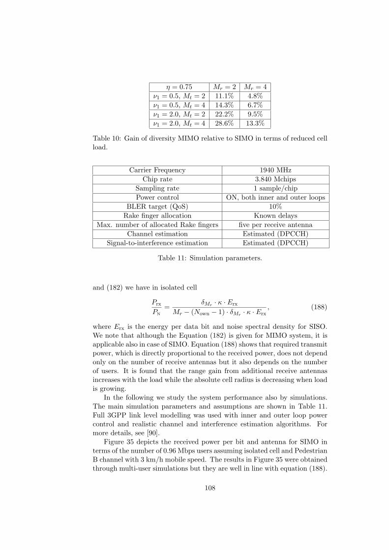
η = 0.75 Mr = 2 Mr = 4ν1 = 0.5, Mt = 2 11.1% 4.8%ν1 = 0.5, Mt = 4 14.3% 6.7%ν1 = 2.0, Mt = 2 22.2% 9.5%ν1 = 2.0, Mt = 4 28.6% 13.3%

Table 10: Gain of diversity MIMO relative to SIMO in terms of reduced cellload.

Carrier Frequency 1940 MHzChip rate 3.840 Mchips

Sampling rate 1 sample/chipPower control ON, both inner and outer loops

BLER target (QoS) 10%Rake finger allocation Known delays

Max. number of allocated Rake fingers five per receive antennaChannel estimation Estimated (DPCCH)

Signal-to-interference estimation Estimated (DPCCH)

Table 11: Simulation parameters.

and (182) we have in isolated cell

Prx

PN

=δMr · κ · Erx

Mr − (Nown − 1) · δMr · κ · Erx, (188)

where Erx is the energy per data bit and noise spectral density for SISO.We note that although the Equation (182) is given for MIMO system, it isapplicable also in case of SIMO. Equation (188) shows that required transmitpower, which is directly proportional to the received power, does not dependonly on the number of receive antennas but it also depends on the numberof users. It is found that the range gain from additional receive antennasincreases with the load while the absolute cell radius is decreasing when loadis growing.

In the following we study the system performance also by simulations.The main simulation parameters and assumptions are shown in Table 11.Full 3GPP link level modelling was used with inner and outer loop powercontrol and realistic channel and interference estimation algorithms. Formore details, see [90].

Figure 35 depicts the received power per bit and antenna for SIMO interms of the number of 0.96 Mbps users assuming isolated cell and PedestrianB channel with 3 km/h mobile speed. The results in Figure 35 were obtainedthrough multi-user simulations but they are well in line with equation (188).

108

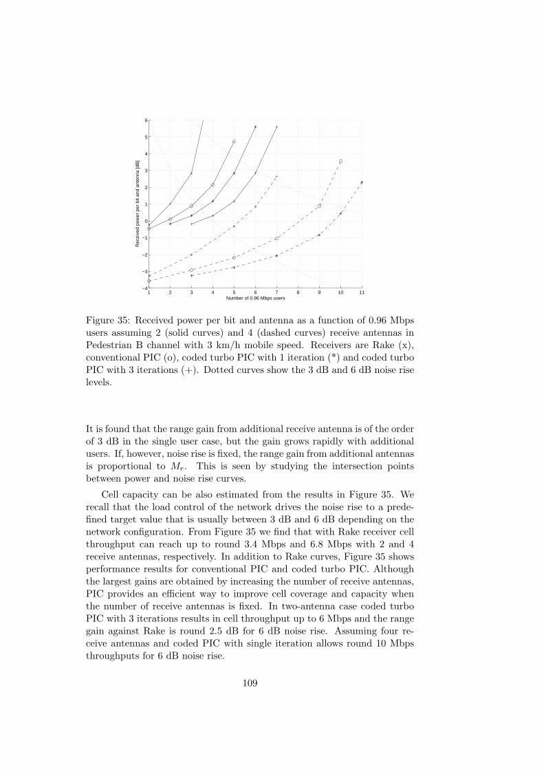
1 2 3 4 5 6 7 8 9 10 11−4

−3

−2

−1

0

1

2

3

4

5

6

Number of 0.96 Mbps users

Rec

eive

d po

wer

per

bit

and

ante

nna

[dB

]

Figure 35: Received power per bit and antenna as a function of 0.96 Mbpsusers assuming 2 (solid curves) and 4 (dashed curves) receive antennas inPedestrian B channel with 3 km/h mobile speed. Receivers are Rake (x),conventional PIC (o), coded turbo PIC with 1 iteration (*) and coded turboPIC with 3 iterations (+). Dotted curves show the 3 dB and 6 dB noise riselevels.

It is found that the range gain from additional receive antenna is of the orderof 3 dB in the single user case, but the gain grows rapidly with additionalusers. If, however, noise rise is fixed, the range gain from additional antennasis proportional to Mr. This is seen by studying the intersection pointsbetween power and noise rise curves.

Cell capacity can be also estimated from the results in Figure 35. Werecall that the load control of the network drives the noise rise to a prede-fined target value that is usually between 3 dB and 6 dB depending on thenetwork configuration. From Figure 35 we find that with Rake receiver cellthroughput can reach up to round 3.4 Mbps and 6.8 Mbps with 2 and 4receive antennas, respectively. In addition to Rake curves, Figure 35 showsperformance results for conventional PIC and coded turbo PIC. Althoughthe largest gains are obtained by increasing the number of receive antennas,PIC provides an efficient way to improve cell coverage and capacity whenthe number of receive antennas is fixed. In two-antenna case coded turboPIC with 3 iterations results in cell throughput up to 6 Mbps and the rangegain against Rake is round 2.5 dB for 6 dB noise rise. Assuming four re-ceive antennas and coded PIC with single iteration allows round 10 Mbpsthroughputs for 6 dB noise rise.

109

0 1 2 3 4 5 6 7 8−7

−6

−5

−4

−3

−2

−1

0

1

2

3

4

Data rate [Mbps]

Rec

eive

d po

wer

per

bit

and

ante

nna

[dB

]

Figure 36: Received power per bit and antenna as a function of data rateassuming Rake with 2 (solid curves), 4 (dashed curves) and 8 (dashed anddotted curves) receive antennas in Vehicular A channel with 30 km/h mobilespeed. Numbers of transmit antennas are 1 (x), 2 (o) and 3 (*). Dottedcurve shows the 3 dB noise rise level.

We recall from (185) and (186) that the effect of PIC can be modeledthrough the efficiency β. This parameter is not constant but depends on cellconditions such as the number of users and channel model. According tosimulations the efficiency for uncoded PIC is round 0.4 at maximum whilecoded PIC with turbo receiver can provide maximum efficiency of round 0.7.

Figure 35 shows the performance for SIMO configuration. However, theperformance for information MIMO can be deduced from the same figureby setting the data rate to Mt × 0.96 Mbps and scaling the number ofusers accordingly. In the analysis this equivalence is seen in equation (183).Thus, there is no throughput gain at the cell level from information MIMOfor low user data rates. Instead, the performance may suffer, because user’spilot power is divided between multiple transmit antennas which deteriorateschannel estimation in the receiver.

The benefits of information MIMO become visible with high user datarates. The main reason for the superiority of information MIMO to SIMOand diversity MIMO is that in information MIMO high data rates can beobtained without heavy code puncturing because independent data streamsare transmitted from separate antennas. Both SIMO and diversity MIMOface serious performance degradation when effective code rate increases dueto puncturing. We note that adaptive modulation and coding in uplink is

110

not supported in UTRA FDD specification, and therefore code puncturingcannot be avoided when SIMO and diversity MIMO are used on high datarates.

Figure 36 shows the received power per bit and antenna in Vehicular Achannel with 30 km/h mobile speed assuming information MIMO and Rakereceiver. Six multi-codes of spreading factor 4 were applied for data rateshigher than 2 Mbps. Data rates higher than Mt × 2 Mbps were generatedby using the code puncturing. It is found that additional transmit antennasprovide a remarkable performance gain when base station has 4 or 8 receiveantennas. Especially in case of 8 receive antennas the gain from the secondand the third data stream is large and data rates up to 7.5 Mbps are obtainedwith 3 dB noise rise. On the other hand, with two receive antennas channelestimation errors slightly degrade the system performance when the seconddata stream is added. For low data rates this phenomenon is also visiblewhen Mr > 2. Besides the channel estimation errors the poor orthogonalityproperties of different scrambling codes also have a negative impact to thesystem performance. Figure 36 also shows the detrimental effect of codepuncturing. Especially in SIMO curves, rapid degradation in performanceis clearly noticeable when data rate exceeds 2 Mbps.

111

7 Conclusions

It has been known for quite some time that in order to communicate effi-ciently over the wireless channel, one should exploit multi-path diversity bybenefiting from independent fading propagation paths. This led to the devel-opment of efficient open-loop (OL) and closed-loop (CL) transmit diversitysolutions with the idea of enhancing capacity by means of taking advantageof the spatial diversity available in the channel. In Section 3 we analyzedCL extended mode 1 (e-mode 1) and extended mode 2 (e-mode 2) that weredesigned based on universal terrestrial radio access (UTRA) frequency di-vision duplex (FDD) CL mode 1 and 2. Although being suboptimal thesealgorithms are efficient and at the same time they admit analysis in termsof signal to noise ratio (SNR) gain, link capacity and bit error probability(BEP).

Results of the analysis in Section 3 show that both e-mode 1 and e-mode2 clearly outperform transmitter selection combining (TSC) that is used asa reference. Furthermore, by e-mode 2 it is possible to achieve almost thesame performance as with perfect channel state information (CSI). Resultsindicate that in the presence of flat fading the SNR gain of both e-mode 1and 2 grow linearly with additional antennas while the SNR gain of TSCadmits only logarithmic growth. In case of two transmit antennas it is shownthat link capacity of CL transmit diversity (TD) methods can be accuratelyapproximated using SNR gain and link capacity formula of maximal ratiocombining. Also the analysis of approximation error is provided. ThroughBEP formulas it is further shown that the studied CL TD methods providefull diversity gain if feedback is error-free. On the contrary, if feedbackis corrupted the slope of the BEP curve in asymptotic SNR region is thesame for multi-antenna CL TD methods and single antenna transmission.Nevertheless, the CL processing provides a constant BEP gain in high SNRregion.

In on-off scheduling (OOS) the selection between positive acknowledg-ment (ACK) and negative acknowledgment (NACK) is based on a SNRthreshold that is known in both transmitter and receiver. In Section 4 OOSwas studied in downlink framework assuming a similar shared channel asin UTRA FDD high-speed downlink packet access (HSDPA). Contrary toHSDPA, in our model only a single user can transmit during each transporttime interval (TTI). Three different physical layer scheduling algorithmswere considered. In system 1, served user is selected irrespective of the CSI.In system 2 all users apply OOS and send ACK or NACK message aftereach TTI based on received relative SNR. Served user is selected amongthose with positive ACK and if no ACK is received in BS, the served user isselected randomly. Finally, in system 3, transmission is assigned to the userwith the best relative channel conditions. Thus, the amount of transmit-ter CSI is one bit per user in system 2 while system 3 applies unquantized

112

feedback. Furthermore, TSC is applied on top of each system.Results in Section 4 indicate that in case of system 2 with OOS there

exists an ACK probability and the corresponding relative SNR thresholdthat maximize the capacity on the shared channel. With optimal ACKprobability system 2 is able to achieve more than 75% of the capacity gainof full SNR feedback, provided that OOS feedback is error-free. It is furthershown that the effect of feedback errors may be crucial to OOS. It turnsout that when ACK probability is small, system 2 is sensitive to feedbackerrors. When feedback error rate is less than 5% performance losses remainat acceptable level in most cases.

Uplink framework presented in Section 5 assumes fast transmit powercontrol (PC) and the OOS threshold corresponds to the relative transmitpower, measured by mobile terminal. Contrary to downlink framework inSection 4, in uplink all users have their control channels on, which enablescontinuous transmit power measurements in terminals. This creates controlchannel overhead that limits the gain of channel-aware scheduling.

The required mean transmit power of OOS was compared to two refer-ence systems that do not exploit CSI. We assumed a model where OOS isapplied only on the data channel while the control channel is on all the time,and fast transmit power control is used on both channels. This model is com-patible with proposed UTRA FDD HSUPA. It was found out that OOS canremarkably reduce the mean transmit power provided that the power ratiobetween control and data channels remains small. On the other hand, itwas shown that the control channel overhead might limit the performanceof OOS although users could tolerate unbounded delays. Furthermore, an-tenna and multi-path diversity reduce the relative gain of OOS. ObtainedOOS gains were also translated into gains in FDD WCDMA coverage andcapacity. We showed how OOS is able to improve service availability byusing a radio link budget example. The achievable capacity gain from OOSstrongly depends on the load and interference conditions in the network, thegain being largest in a heavily loaded system with high inter-cell interferencelevel.

In Section 6 it was shown that the uplink coverage and capacity of UTRAFDD mode can be greatly improved by single-input multiple-output (SIMO)and multiple-input multiple-output (MIMO) transceivers. We studied twoapproaches referred to as diversity MIMO and information MIMO. In theformer case, a single data stream is transmitted and multiple antennas areused to decrease the variance of the received signal and thereby improve thequality of the radio link. In the latter case, multiple transceiver antennasare used for parallel multiplexing, i.e. to transmit several data streamssimultaneously to a user to increase peak data rates.

While the gain from diversity MIMO is noticeable only in the presenceof heavy inter-cell interference, the gain from additional receive antennas isremarkable also in isolated cell. The information MIMO shows its power

113

when high user data rates are needed. This is mostly due to the fact thatheavy code puncturing can be avoided by using the information MIMO.UTRA FDD uplink is not code limited and therefore diversity and informa-tion MIMO can be implemented by allocating additional channelization orscrambling codes to different transmit antennas. Thus, the receiver in basestation can separate the signals from different antennas in code domain andit is not necessary to rely on spatial signatures and space-time code design.This makes the system more robust and receivers can utilize well-knownmulti-user and interference cancellation receivers developed for CDMA sys-tems. Furthermore, these MIMO schemes can be implemented with onlyminor changes to the present specification.

114

References

[1] J. Hamalainen, R. Wichman, “Closed–loop transmit diversity for FDDWCDMA systems,” 34th Asilomar Conference on Signals, Systems andComputers, October 2000.

[2] J. Hamalainen, R. Wichman, “Multiple antenna transmission utilizingside information for WCDMA systems,” The 5th CDMA InternationalConference and Exhibition, Seoul, Korea, November 2000.

[3] J. Hamalainen, R. Wichman, “Feedback schemes for FDD WCDMAsystems in multipath environments,” IEEE Vehicular Technology Con-ference, Rhodes, Greece, May 2001.

[4] J. Hamalainen, R. Wichman, “Performance analysis of closed–looptransmit diversity in the presence of feedback errors,” IEEE Interna-tional Symposium on Personal, Indoor and Mobile Radio Communica-tions, September 2002.

[5] J. Hamalainen, R. Wichman, “Asymptotic bit error probabilities ofsome closed–loop transmit diversity schemes,” IEEE Global Telecom-munications Conference, November 2002.

[6] J. Hamalainen, R. Wichman, “Capacity of generalized UTRA FDDclosed–loop transmit diversity modes,” in preparation.

[7] R. Wichman, J. Hamalainen, “Transmit diversity weight generation forwireless FDD systems with feedback,” IEEE and EURASIP Workshopon Nonlinear Signal and Image Processing, Baltimore, Maryland, USA,June 2001.

[8] J. Hamalainen, R. Wichman, “The effect of feedback delay to the closed-loop transmit diversity in FDD WCDMA,” IEEE International Sym-posium on Personal, Indoor and Mobile Radio Communications, SanDiego, California, September 30–October 3, 2001.

[9] J. Hamalainen, R. Wichman, “Closed–loop transmit diversity for FDDWCDMA in fading channels,” Second Finnish Wireless Communica-tions Workshop, Tampere, Finland, October 2001.

[10] J. Hamalainen, O. Piirainen, R. Wichman, “On the SNR gain of polar-ization matching,” Finnish Wireless Communications Workshop, May2002.

[11] J. Hamalainen, R. Wichman, “On optimality of closed–loop transmitdiversity,” Finnish Wireless Communications Workshop, May 2002.

115

[12] J. Hamalainen, R. Wichman, “On the performance of FDD WCDMAclosed–loop transmit diversity modes in Nakagami and Ricean fadingchannels,” IEEE International Symposium of Spread Spectrum Tech-niques and Applications, Prague, Czech Republic, September 2002.

[13] J. Hamalainen, R. Wichman, T. Kahkonen, J. Hulkkonen, T. Korpi,M. Saily, “On the performance of GERAN transmit diversity schemeswhen employing dual–polarized antennas,” IEEE Vehicular TechnologyConference, Korea, April 2003.

[14] J. Hulkkonen, T. Kahkonen, J. Hamalainen, T. Korpi, M. Saily, “Ca-pacity gain from transmit diversity methods in limited bandwidthGERAN networks,” IEEE Vehicular Technology Conference, Korea,April 2003.

[15] J. Hamalainen, R. Wichman, “On the site selection diversity transmis-sion,” IEEE International Symposium on Personal, Indoor and MobileRadio Communications, September 2003.

[16] J. Hamalainen, R. Wichman, T. Korhonen: Chapter “Multi-channeladaptive beam-forming” in book “Adaptive Antenna Arrays”, ed. by S.Chandran, Springer Verlag, 2004.

[17] J. Hamalainen, R. Wichman, “Capacities of physical layer schedulingstrategies on a shared link,” Wireless Personal Communications, vol.39 no. 1, pp. 115-134, October 2006.

[18] J. Hamalainen, R. Wichman, “Bit error probabilities in a two–ratecommunication system,” IEEE International Conference on Commu-nications, May 2003.

[19] J. Hamalainen, R. Wichman, “Quantization of channel quality indicatorin maximum SNR scheduling,” Nordic Radio Symposium, August 2004.

[20] J. Hamalainen, R. Wichman, “Combining multiuser diversity andWCDMA transmit diversity modes,” IEEE Nordic Signal ProcessingSymposium, October 2002.

[21] J. Hamalainen, R. Wichman, “Performance of transmit time selectiondiversity in multipath fading channels,” The 6th International Sympo-sium on Wireless Personal Multimedia Communications, October 2003.

[22] J. Hamalainen, R. Wichman, “Performance of multiuser diversity inthe presence of feedback errors,” IEEE International Symposium onPersonal, Indoor and Mobile Radio Communications, September 2004.

116

[23] G. Corral-Briones, A. A. Dowhuszko, J. Hamalainen, R. Wichman,“Achievable data rates for multiple transmit antenna broadcast chan-nels with closed–loop transmit diversity modes,” IEEE InternationalConference on Communications, May 2005.

[24] G. Corral-Briones, A. A. Dowhuszko, J. Hamalainen, R. Wichman,“Downlink multiuser scheduling algorithm with FDD WCDMA closed–loop feedback information,” IEEE Vehicular Technology Conference,May 2005.

[25] J. Hamalainen, R. Wichman, “The effect of control channel overheadupon physical layer scheduling,” Wireless Personal Communications,vol. 35, no. 4, pp. 337-352, December 2005.

[26] J. Hamalainen, K. Pajukoski, E. Tiirola, R. Wichman, J. Ylitalo, “Onthe performance of multiuser MIMO in UTRA FDD uplink,” EURASIPJournal on Wireless Communications and Networking, Special Issue onMultiuser MIMO Networks, Vol. 2, pp. 297–308, 2004.

[27] J. Hamalainen, K. Pajukoski, E. Tiirola, R. Wichman, J. Ylitalo,“MIMO performance in UTRA FDD uplink,” IEEE International Sym-posium of Spread Spectrum Techniques and Applications, September2004.

[28] J. Hamalainen, R. Wichman, M. Kuusela, E. Tiirola, K. Pajukoski:Chapter “Multiuser MIMO for UTRA FDD” in book “MIMO antennatechnology for wireless communications”, ed. by G. Tsoulos, CRC Press,2006.

[29] E. Tiirola, J. Hamalainen, K. Pajukoski, J. Ylitalo, “Performance anal-ysis for some practical high data rate extensions of UTRA FDD uplink,”IEEE Vehicular Technology Conference, September 2004.

[30] J. Hamalainen, R. Wichman, “On the correlations between dual–polarized base station antennas,” IEEE Global TelecommunicationsConference, November 2003.

[31] J. Ylitalo, J. P. Nuutinen, J. Hamalainen, T. Jamsa, M. Hamalainen,“Multi–dimensional wideband radio channel characterization for 2-6GHz band,” Wireless World Research Forum, WWRF11 Meeting inOslo, June 2004.

[32] J. Hamalainen, S. Savolainen, R. Wichman, K. Ruotsalainen, J. Ylitalo,“Integral equation formulation for scatter density problem,” ElectronicsLetters, vol. 41, no. 2, pp. 82-83, January 2005.

117

[33] J. Hamalainen, J. P. Nuutinen, R. Wichman, J. Ylitalo, T. Jamsa,“Analysis and measurements for indoor polarization MIMO in 5.25 GHzband,” IEEE Vehicular Technology Conference, May 2005.

[34] J. Hamalainen, S. Savolainen, R. Wichman, K. Ruotsalainen, J. Ylitalo,“On solution of scatter density in geometry–based channel models,”accepted to IEEE Trans. Wireless Commun., June 2005.

[35] 3GPP Technical specification 25.201, “UTRA physical layer generaldescription,” ver. 6.2.0, June 2005.

[36] 3GPP Technical specification 25.213, “Spreading and modulation,” ver.6.4.0, September 2005.

[37] Holma, H. and A. Toskala (eds.), WCDMA for UMTS, Wiley, thirdedition, 2004.

[38] 3GPP Technical specification 25.211, “Physical channels and mappingof transport channels onto physical channels (fdd),” ver. 6.6.0, Septem-ber 2005.

[39] 3GPP Technical report 25.848, “Physical layer aspects of UTRA highspeed downlink Packet Access,” ver. 4.0.0, April 2001

[40] 3GPP Technical report 25.899, “HSDPA enhancements,” ver. 6.1.0,September 2005.

[41] R. Knopp, P. Humblet, “Information capacity and power control in sin-gle cell multiuser communications,” International Conference on Com-munications, June 1995.

[42] R. Knopp, Coding and multiple–access over fading channels, Ph.D. dis-sertation, Ecole Polytehnique Federale de Lausanne, 1997.

[43] K. Pedersen, P. Mogensen, and J. Ramiro-Moreno, “Application andperformance of downlink beamforming techniques in UMTS,” IEEECommun. Mag., vol. 41, no. 10, pp. 134–143, 2003.

[44] E. Tiirola and J. Ylitalo, “Comparison of beam–forming and diversitytechniques in terms of UTRA FDD uplink capacity,” in Nordic RadioSymposium, August 2004.

[45] S. Alamouti, “A simple transmitter diversity technique for wireless com-munications,” IEEE J. Select. Areas Commun., vol. 16, no. 8, pp. 1451–1458, October 1998.

[46] 3GPP Technical specification 25.214, “Physical layer procedures(FDD),” ver. 4.6.0, April 2003.

118

[47] 3GPP Technical report 25.869, “Transmitter diversity solutions for mul-tiple antennas (withdrawn from rel. 6),” ver. 1.2.0, September 2003.

[48] V. Tarokh, N. Seshadri, A. R. Calderbank, “Space–time codes for highdata rate wireless communications”, IEEE Trans. Inform. Theory, vol.44, no. 2, pp. 744-765, March 1998.

[49] V. Tarokh, H. Jafarkhani, A. R. Calderbank, “Space–time block codesfrom orthogonal designs”, IEEE Trans. Inform. Theory, vol. 45, no. 5,pp. 1456-1467, July 1999.

[50] A. Narula, M. J. Lopez, M. D. Trott, G. W. Wornell, “Efficient useof side information in multiple–antenna data transmission over fadingchannels,” IEEE J. Select. Areas Commun., vol. 17, no. 8, pp. 1423-1436, October 1998.

[51] M. Sandell, “Analytical analysis of transmit diversity in WCDMA onfading multipath channels”, IEEE International Symposium on Per-sonal, Indoor and Mobile Radio Communications, 1999.

[52] W. C. Y. Lee, “Estimate of channel capacity in Rayleigh fading en-vironment,” IEEE Trans. Veh. Technol., vol. 39, pp. 187–190, August1990.

[53] A. Goldsmith, P. Varaiya, “Capacity of fading channels with channelside information,” IEEE Trans. Inform. Theory, vol. 43, pp. 1896–1992,November 1997.

[54] M-S. Alouini, A. J. Goldsmith, “Capacity of Rayleigh fading channelsunder different adaptive transmission and diversity–combining tech-niques,” IEEE Trans. Veh. Technol., vol. 48, no. 4, pp. 1165–1181,July 1999.

[55] R. W. Health, A. Paulraj, “A simple scheme for transmit diversityusing partial channel feedback,” 32th Asilomar Conference on Signals,Systems and Computers, pp. 1073–1078, 1998.

[56] E. Onggosanusi, A. Gatherer, A. Dabak, S. Hosur, “Performance analy-sis of closed–loop transmit diversity in the presence of feedback delay,”IEEE Trans. Commun., vol. 49, no. 9, pp. 1618–1630, September 2001.

[57] J. Choi, “Performance analysis for transmit antenna diversitywith/without channel information,” IEEE Trans. Veh. Technol., vol.51, no. 1, pp. 101–113, January 2002.

[58] E. Visotsky, U. Madhow, “Space–time transmit precoding with imper-fect feedback,” IEEE Trans. Inform. Theory, vol. 4, no. 6, pp. 2632–2639, September 2001.

119

[59] S. Miller, J. Shapira, “Transmission considerations for polarization–smart antennas,” in IEEE Vehicular Technology Conference, May 2001.

[60] S. Miller, J. Shapira, “A novel polarization smart antennas,” in IEEEVehicular Technology Conference, May 2001.

[61] B. Raghothaman, G. Mandyam, R. T. Derryberry, “Performance ofclosed loop transmit diversity with feedback delay, 34th Asilomar Con-ference on Signals, Systems and Computers, pp. 102–105, October 2000.

[62] C. W. Sung, S. C. Ip, K. K. Leung, “A simple algorithm for closed-loop transmit diversity with a low-data-rate feedback channel,” IEEEPacific Rim Conference on Communications, Computers and SignalProcessing, pp. 384-387, 2005.

[63] K. Kiran Mukkavilli, A. Sabharwal, E. Erkip, B. Aazhang, “On beam-forming with finite rate feedback in multiple-antenna systems,” IEEETrans. Inform. Theory, vol. 49, no. 10, pp. 2562-2579, 2003.

[64] D. J. Love, R. W. Heath, T. Strohmer, “Grassmannian beamforming formultiple-input multiple-output wireless systems,” IEEE Trans. Inform.Theory, vol. 49, no. 10, pp. 2735-2747, 2003.

[65] W. C. Jakes (ed), Microwave mobile communications, IEEE Press,1974.

[66] J. Lieblein, “On moments of order statistics from the Weibull distribu-tion,” Ann. Math. Stat. 26, pp. 330–333, 1955.

[67] M. Nakagami, “Statistical characters of short–wave fading,” J. IEICEJap., vol. 27, no. 2, pp. 145-150, February 1943.

[68] M. Nakagami, “The m-distribution-A general formula of intensitydistri- bution of rapid fading,” in Statistical Methods of Radio WavePropagation, W. C. Hoffman Ed. New York: Pergamon Press, pp. 3–36, 1960.

[69] M. Abramowitz and I. Stegun, Eds., Handbook of mathematical func-tions. Washington DC: National Bureau of Standards, 1972.

[70] 3GPP Technical report 25.896, “Feasibility Study for Enhanced Uplinkfor UTRA FDD,” ver. 6.0.0, March 2004.

[71] J. Proakis, Digital Communications. McGraw-Hill, 1995.

[72] P. Viswanath, D.N.C. Tse, and R. Laroia, “Opportunistic beam-forming using dumb antennas,” IEEE Trans. Inform. Theory, vol. 48,no. 6, pp. 1277–1294, June 2002.

120

[73] M. Johansson, “Benefits of multiuser diversity with limited feedback,”IEEE International Workshop on Signal Processing Advances in Wire-less Communications, 2003.

[74] F. Floren, O. Edfors, and B.-A. Molin, “The effect of feedback quan-tization on the throughput of a multiuser diversity scheme,” GlobalTelecommunications Conference, vol. 1, pages 497–501, 2003.

[75] S. Zhou, Z. Wang, G. B. Giannakis, “Quantifying the power loss whentransmit beamforming relies on finite-rate feedback,” Trans. WirelessCommun., vol. 4, no. 4, pp. 1948-1957, 2005.

[76] D. Gesbert and S. Alouini, “How much feedback is multi–user diversityreally worth?,” IEEE International Conference on Communications,Paris, France, 2004.

[77] L. T. Berger, T. E. Kolding, J. Ramiro-Moreno, P. Ameigeiras, L. Schu-macher, P. E. Mogensen, “Interaction of transmit diversity and propor-tional fair scheduling,” IEEE Vehicular Technology Conference, April2003.

[78] J. Ramiro-Moreno, K. I. Pedersen, P. E. Mogensen, “Network perfor-mance of transmit and receive antenna diversity in HSDPA under dif-ferent packet scheduling strategies,” IEEE Vehicular Technology Con-ference, April 2003.

[79] R. Gonzali, R. M. Buehrer, B. D. Woerner, “The impact of multiuserdiversity on space–time block coding,” IEEE Commun. Letters, vol. 7,no. 5, May 2003.

[80] J. Torrance, L. Hanzo, “Upper bound performance of adaptive modu-lation in a slow Rayleigh fading channel,” Electronics Letters, vol. 32,no. 8, pp. 718-719, April 1996.

[81] A. Rangarajan and V. Sharma, “Achieving exponential diversity or-der in Rayleigh fading channels,” National Communication Conference(NCC) 2004, Bangalore, India, 2004.

[82] A. M. Viterbi, A. J. Viterbi, “Erlang capacity of power controlledCDMA system,” IEEE J. Select. Areas Commun. vol. 11, no. 6, pp.892–900, August 1993.

[83] A. J. Viterbi, A. M. Viterbi, E. Zehavi, “Other–cell interference incellular power-controlled CDMA,” IEEE Trans. Commun. vol. 42, Issue234, Part 3, pp. 1501–1504, February/March/April 1994.

[84] A. Viterbi, CDMA: Principles of spread spectrum communication,Addison-Wesley, Reading, Mass, USA, 1995.

121

[85] Ariyavisitakul, S. and L. Chang, “Signal and interference statistics of aCDMA system with feedback power control,” IEEE Trans. Commun.vol. 41 no. 11, pp. 1626–1634, 1993.

[86] D. Raja, A. Sabharwal, B. Aazhang, “Impact of multiple access onuplink scheduling,” IEEE Information Theory Workshop, September2001.

[87] K. Lau, “Analytical framework for multiuser uplink MIMO space–timescheduling design with convex utility functions,” IEEE Trans. WirelessCommun., vol. 3, no. 5, pp. 1832–1843, September 2004.

[88] J. Meilong, V. K. Lau, “Performance analysis of proportional fair uplinkscheduling with channel estimation error in multiple access system,”IEEE International Symposium on Personal, Indoor and Mobile RadioCommunications, September 2004.

[89] ITU, “Guidelines for evaluation of radio transmission technologies forIMT–2000,” Recommendation ITU-R.M.1225, 1997.

[90] 3GPP Technical specification 25.104, “BS Radio Transmission and Re-ception (FDD),” ver. 7.0.0, June 2005.

[91] Hata, M., “Empirical formula for propagation loss in land mobile radioservices,” IEEE Trans. Veh. Technol. VT-29, no. 3, 1980.

[92] Okumura, Y., E. Ohmori, T. Kawano, and K. Fukuda, “Field strengthand its variability in the VHF and UHF land mobile service,” ReviewElectronic Communication Lab. vol. 16 no. 9-10, pp. 825–873, 1968.

[93] Laiho, J., A. Wacker, and T. Novosad, Radio network planning andoptimization for UMTS, Wiley, 2002.

[94] G. J. Foschini, “Layered space–time architecture for wireless commu-nication in a fading environment when using multi-element antennas,”Bell Labs. Tech. J., pp. 41–59, 1996.

[95] G. J. Foschini, M. J. Gans, “On limits of wireless communications in afading environment when using multiple antennas,” Wireless PersonalCommunications, vol. 6, pp. 311–335, March 1998.

[96] E. Telatar, “Capacity of multi-antenna Gaussian channels,” EuropeanTrans. Telecomm., vol. 10, no. 6, pp. 585–595, Nov/Dec 1999, based onAT& T Bell Laboratories, Internal Tech. Memo, June 1995.

[97] D. Gesbert, M. Shafi, D-S. Shiu, P. J. Smith, A. Naguib, “From theoryto practise: An overview of MIMO space-time coded wireless systems,”IEEE J. Select. Areas Commun., vol. 21, no. 3, pp. 281-302, April 2003.

122

[98] F. Horlin, L. Vandendorpe, “MU-MIMO channel adapted precoding forMAI/ISI-free uplink burst transmission,” IEEE Trans. Commun., vol.52, no. 1, pp. 100–109, January 2004.

[99] H. Boche, M. Wiczanowski, “Optimal transmit covariance matrices forMIMO high speed uplink packet access,” IEEE Wireless Communica-tions and Networking Conference, March 2004.

[100] 3GPP Technical report 25.867, “Multiple-input multiple-output inUTRA (withdrawn from release 6),” ver. 1.7.1, October 2005.

[101] Y. Sanada and Q. Wang, “A co-channel interference cancellation tech-nique using orthogonal convolutional codes,” IEEE Trans. Commun.,vol. 44, no. 5, 1996.

[102] H. C. Kwon, K. J. Kim, B. H. Park, and K. C. Whang, “Turbo codedCDMA system with an interference cancellation technique,” IEICETrans. Commun., vol. E81-B, no. 12, 1998.

[103] S.G. Wilson, “Magnitude/phase quantization of independent Gaussianvariates”, IEEE Trans. Commun., vol. 28, November 1980, pp. 1924-1929.

123