Performance Analysis of Cell Rate Monitoring Mechanisms in ATM Systems · Performance Analysis of...

8

Performance Analysis of Cell Rate Monitoring Mechanisms in ATM Systems

M. Ritter, P. Tran-Cia

University of Wiirzburg, Institute of Computer Science Am Hubland, D - 97074 Wiirzburg, Germany Tel: +49 931 888 5505, Fax: +49 931 888 4601 e-mail: [email protected]

Abstract

The control of cell processes plays a central role in ATM network management and strongly influences the overall system overload behavior and the quality of service. One of the crucial control functions is the usage parameter control according to the user-network contract for a connection. Due to the slotted time of the ATM cell process discretetime models are suited for performance analysis. In this paper we first present queueing models operating in discrete-time for the cell rate monitoring, where arbitrary renewal cell input processes are taken into account. Subsequently cell processes of ON/OFF-type are considered, where the lengths of ON- and OFF-phases can be arbitrarily distributed. Numerical results are discussed aiming the proper choice of the source traffic descriptor parameter values like cell delay variation tolerance, sustainable cell rate and burst tolerance for different cell process characteristics to be enforced.

Keywords

Asynchronous Transfer Mode, Consecutive Cell Loss, Cell Rate Monitoring, DepartureProcess, Discrete-Time Analysis, Generic Cell Rate Algorithm, ON/OFF-Sources

T. Hasegawa et al. (eds.), Local and Metropolitan Communication Systems© Springer Science+Business Media Dordrecht 1995

130 Part Three ATM Multiplexing

1 Introduction to cell rate monitoring algorithms

The Usage Parameter Control (UP C) is one of the most important tasks for the ATM network management. UPC is defined as the set of actions performed by the network to monitor and control traffic at the user access. The aim of UPC is to prevent the malicious or unintentional excessive usage of network resources which would lead to Quality of Service (QOS) degradation. One of the possible QOS parameters which the network commits to meet (if a user complies with its traffic contract) is the cell loss ratio. Each connection can require up to two cell loss ratio objectives, one for each Cell Loss Priority (CLP) class, i.e. for CLP=O (high priority) and CLP=1 (low priority) cells.

At connection setup, mandatory parameters are the Peak Cell Rate (PCR) for CLP=O+1 and the Cell Delay Variation (CDV) tolerance. In addition, the Sustainable Cell Rate (SCR) and the Burst Tolerance can be described optionally (if used, they must be specified together [1, 5]). The SCR of an ATM connection is an upper bound on the Average Cell Rate (ACR) of this connection. It is to be specified only for VBR services, since PCR and SCR are equal for CBR services. By the specification of the SCR of a connection, the network operator may allocate less network resources (but still meet the required QOS) than if only the PCR would be specified. For any source type, the following relation holds irrespectively of the time scale t over which these parameters are defined:

PCRt s; SCRt s; ACRt (1)

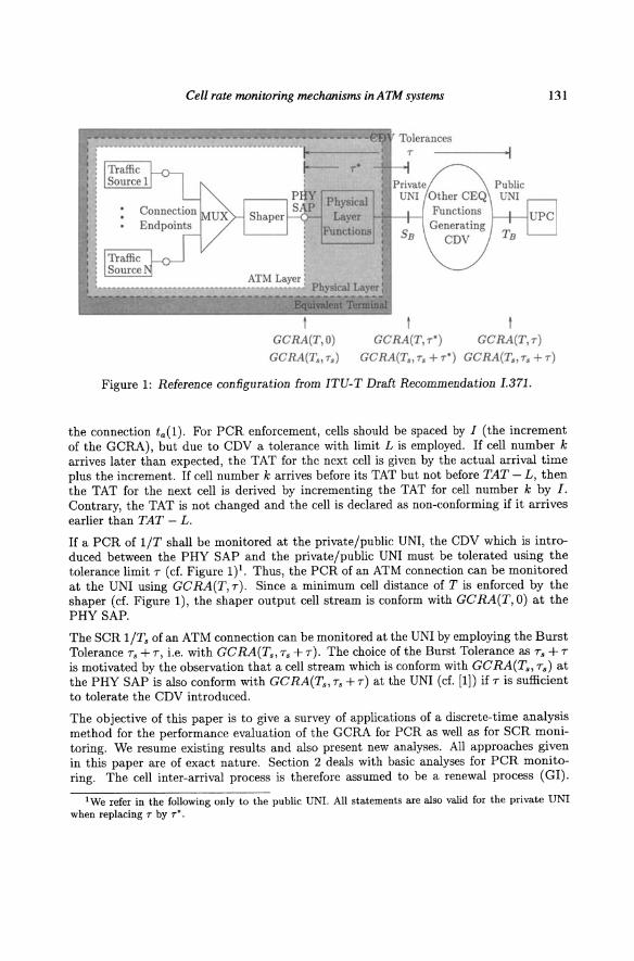
PCR and SCR are defined at the Physical Layer Service Access Point (PRY SAP) and the conformance of cell streams according to them is monitored at the private/public User Network Interface (UNI). The corresponding reference configuration from ITU-T Draft Recommendation 1.371 [14], which was adopted by the ATM Forum [1], is depicted in Figure l.

Cells of traffic streams from different connections are multiplexed together and then pass through a shaper to reduce CDV introduced by multiplexing. But after the traffic shaping, CDV is introduced again between the PRY SAP and the private/public UNI. Since cell stream conformance according to the negotiated PCR and SCR is monitored at the private/public UNI, CDV must be tolerated using the CDV tolerance.

Several algorithms have been suggested to monitor cell streams. These are for example the Leaky Bucket, the Jumping Window Mechanism, the Triggered Jumping Window Mechanism or the Exponentially Weighted Moving A verage Mechanism. Descriptions and performance comparisons ofthese algorithms can be found for example in [6, 7, 17, 18, 19].

For ATM networks however, the Generic Cell Rate Algorithm (GCRA) for PCR/SCR monitoring was proposed by the ATM Forum [1]. There are two versions of the GCRA, namely the Virtual Scheduling Algorithm and the Continuous-State Leaky Bucket Algorithm, which are equivalent in that sense that both versions declare the same cells of a cell stream as conforming or non-conforming. We refer in this paper to the Virtual Scheduling Algorithm which is depicted in Figure 2. This algorithm was proposed first by the ITU-T Draft Recommendation 1.371 [14] to monitor the PCR.

The GCRA uses a Theoretical Arrival Time (TAT) for the earliest time instant the next cell is expected to arrive. The TAT is initialized with the arrival time of the first cell of

Cell rate monitoring mechanisms inATM systems 131

ATM Layer ....... --........ -.-....... ----..... - ..... ~ Physical Lay"r:

Bqalvalent TermlDal

GCRA(T,O) GCRA(T TO) GCRA(T T) GCRA(T., T.) GCRA(T" T. + TO) GCRA(T .. T. + T)

Figure 1: Reference configuration from ITU-T Draft Recommendation 1.371 .

the connection ta(l). For PCR enforcement , cells should be spaced by I (the increment of the GCRA) , but due to CDV a tolerance with limit L is employed. If cell number k arrives later than expected, the TAT for the next cell is given by the actual arrival time plus the increment. If cell number k arrives before its TAT but not before TAT - L, then the TAT for the next cell is derived by incrementing the TAT for cell number k by I. Contrary, the TAT is not changed and the cell is declared as non-conforming if it arrives earlier than TAT - L .

If a PCR of l/T shall be monitored at the private/public UNI, the CDV which is introduced between the PRY SAP and the private/public UNI must be tolerated using the tolerance limit T (cf. Figure 1)1. Thus, the PCR of an ATM connection can be monitored at the UNI using GCRA(T, T). Since a minimum cell distance of T is enforced by the shaper (cf. Figure 1), the shaper output cell stream is conform with GCRA(T,O) at the PRY SAP.

The SCR l/Ts of an ATM connection can be monitored at the UNI by employing the Burst Tolerance Ts + T, i.e. with GCRA(T., Ts + T). The choice of the Burst Tolerance as Ts + T

is motivated by the observation that a cell stream which is conform with GCRA(T., Ts) at the PRY SAP is also conform with GC RA(T., Ts + T) at the UNI (cf. [1]) if T is sufficient to tolerate the CDV introduced.

The objective of this paper is to give a survey of applications of a discrete-time analysis method for the performance evaluation of the GCRA for PCR as well as for SCR monitoring. We resume existing results and also present new analyses. All approaches given in this paper are of exact nature. Section 2 deals with basic analyses for PCR monitoring. The cell inter-arrival process is therefore assumed to be a renewal process (GI).

1 We refer in the following only to the public UNI. All statements are also valid for the private UNI when replacing T by T*.

132 Part Three ATM MUltiplexing

arrival of cell k at time ta (k)

next cell

non-conforming

cell t--_ye_s-< ta(k) < TAT - L

no

TAT = max(ta(k), TAT) + I conforming cell

Figure 2: GCRA(I, L) as Virtual Scheduling Algorithm.

Due to the shaping function, the nature of a single traffic stream at the PRY SAP is of ON/OFF-type with fixed distances between two succeeding cells in the ON-phases. Since the SCR is defined at the PRY SAP, the assumption of sllr.h an ON/OFF process is more appropriate to derive proper choices of the source traffic descriptor parameter values for SCR monitoring. To deal with this, we present in Section 3 an analysis of the GCRA with ON/OFF-input traffic which is based on the results derived in Section 2. Numerical results are given for illustration. The paper ends with a conclusion and an outlook to further research activities.

2 Basic GCRA modeling

In this section we address performance measures of the GCRA like the cell rejection probability, the cell inter-departure time distribution and the consecutive cell loss distribution if cell streams which follow a GI process are monitored. The analyses are based on the G I / G I /1 queueing model with bounded delay and are of exact nature. First, we briefly present a discrete-time analysis of this queueing system and then focus on analytical approaches of the GCRA using these results.


2.1 The GI /GI /1 queue with bounded delay

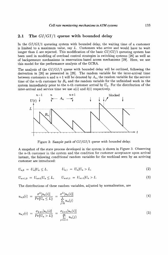
In the GI IGI II queueing system with bounded delay, the waiting time of a customer is limited to a maximum value, say L. Customers who arrive and would have to wait longer than L are rejected. This modification of the basic GI IGI II queueing system has been used in modeling of overload control strategies in switching systems [26] as well as of backpressure mechanisms in reservation-based access mechanisms [29]. Here, we use this model for the performance analysis of the GCRA.

The analysis of the GI IGI II queue with bounded delay will be outlined, following the derivation in [26] as presented in [28]. The random variable for the inter-arrival time between customers nand n+ 1 will be denoted by An, the random variable for the service time of the n-th customer by Bn and the random variable for the unfinished work in the system immediately prior to the n-th customer arrival by Un. For the distribution of the inter-arrival and service time we use a(i) and b(i) respectively.

n-l blocked

U(t) ~ ~ ~I ~

L -.-----------

Figure 3: Sample path of GI IGI II queue with bounded delay.

A snapshot of the state process developed in the system is shown in Figure 3. Observing the n-th customer in the system and the condition for customer acceptance upon arrival instant, the following conditional random variables for the workload seen by an arriving customer are introduced:

The distributions of these random variables, adjusted by normalization, are

Un,! (i) O'L+dun(i)] Pr{Un>L}

lJ"L[un(i)] L L: un(j) j=O

lJ"L+dun(i)]

f un(j) j=L+!

(2)

(3)

(4)

(5)


where u m (.) and O'm(.) are operators which truncate parts of the probability distribution function. The results of these operations are un normalized distributions defined by

17m [x(i)] = { ~(i) iSm (6)

i >m

17m [x(i)] = { ~(i) : i <m

(7) : i '2 m

Observing the development of the process (cf. Figure 3) together with the maximum delay L, the following relationships between the random variables and their distributions are obtained:

• Un S L: customer acceptance

Un +1,O un+1,o(i)

max{O, Un,o + En - An}

'Il'o[un,o(i) * b(i) * a( -i)],

• Un > L: customer rejection

Un+1,l un+1,l(i)

max{O, Un,l - An}

'Il'o [Un,l (i) * a( -i)],

where the operator 'Il'of.] is defined by

'Il'o[x(i)] { x(i)

~=~oo x(j)

i>O

i=O

i<O

The distribution of the workload seen by the (n + 1)-th customer is

un+l(i) = Pr{Un S L}· un+1,o(i) + Pr{Un > L}· un+1,l(i).

(8)

(9)

(10)

(11)

From equations (8), (9) and (11), we finally arrive at a recursive relation to calculate the workload at arrival epochs of customers

'Il'o [uL[un(i)] *b(i) U(-i)] + 'Il'o[uL+dun(i)] *a(-i)]

'Il'o [( uL[un(i)] * b( i) + UL+1 [un( i)]) * a( -i)].

(12)

Using equation (12), an iterative algorithm to calculate the workload prior to customer arrivals can be found. The computational diagram is depicted in Figure 4.


Figure 4: Computational diagram for GI /GI /1 queue with bounded delay.

Finally, the customer rejection probability in statistical equilibrium is

00

p L u(j). (13) j=L+l

This probability will be used to characterize the cell blocking phenomenon in the next section.

2.2 Cell rejection analysis

In ATM networks, the cell rejection probability is one of the most important QOS parameters which must be guaranteed by the network as long as the traffic source complies with its negotiated traffic contract. Therefore, the UPC function must be dimensioned carefully. Already published studies which are concerned with the dimensioning of the GCRA are e.g. [2, 8, 9, 10, 11, 25].

Using the GI /GI /1 queue with bounded delay as presented above, the GCRA can be modeled easily. Since ATM cells have a fixed length, we deal in the following with the G I / D /1 system with bounded delay. The analytical method we now present was first described in [11], however, based on the GIIX]/D/1 - S queueing model analyzed in [27]. If the service process is of deterministic nature, like in our case, the two queueing systems are equivalent. Therefore, the batch size of the G IIX] / D /1 - S system has to be deterministic and equal to the service time of the G I / D /1 system with bounded delay and the system size S corresponds to the delay bound L.

In the following we briefly resume the analysis in [11] to compute the cell rejection probability of the GCRA(T, r) if cell streams which follow a GI process are monitored. The actual state of the GCRA(T, r) is described by the discrete-time random variable U(t), which represents the remaining time until the next cell is expected to arrive. U(t) can be thought of as the virtual unfinished work. A cell arriving at time to seeing the GCRA(T, r) in state U(to) = j is considered to be conforming for j :S r, otherwise non-conforming. Thus, the state process of the virtual unfinished work of the GC RA(T, r) is identical to the unfinished work process of a G I / D /1 queue with bounded delay. The delay bound is L = r and an arriving cell which is conforming increases U(t) by an amount of T,


the increment parameter of the GCRA(T, T). The inter-arrival time distribution is again denoted by a( i) and since the service time is deterministic and equal to T, we get

b(i) = b(i - T). (14)

Using the analysis presented in Section 2.1, we obtain the following relationships between the random variables and their distributions:

• Un ~ T: customer acceptance

Un +1,O un +1,o(i)

max{O, Un,o + T - An}

7ro[un ,o(i) * b(i - T) * a( -i)].

• Un > T: customer rejection

Un +1,1

U n +1,1 (i)

max{O, Un,1 - An} 7ro[un,l(i) *a(-i)].

(15)

(16)

The system state distribution in equilibrium u(i) can now be derived by using equation (12) iteratively, i.e.

(17)

According to Section 2.1 equation (13), the probability to observe a non-conforming cell Pr is given by

T+T

Pr L u(j). (18) j=T+l

2.3 Cell inter-departure distribution

Now, we focus on the computation of the cell inter-departure time distribution d(i). This distribution is an interesting traffic characteristic, because it can be used e.g. to describe the input traffic of an ATM multiplexer located after the UPC function.

The inter-departure time distribution can be derived in closed form using the distribution for the virtual unfinished work u(i) computed in Section 2.2. The approach we outline in this subsection has been presented first in [12].

The shortest inter-arrival time for which two cells can be accepted by the GCRA(T, T) is T - T slots if T < T and one slot otherwise. Therefore, we get

d(i) = 0 for o ~ i < max{l, T - T}. (19)

Cell rate monitoring mechanisms in ATM systems 137

For i 2: max{l, T - T}, the probability that the cell inter-departure time equals i slots is given by

d(i) = L:Pr{Un = j jj :::; T}' Pr{AE = i}. j

(20)

The first factor in the sum represents the probability that an accepted cell n sees the GC RA(T, T) in state Un = j whereas the second factor is the probability that the sum of the inter-arrival times of rejected cells and of the next accepted cell AE = i.

Since u(i) denotes the equilibrium state distribution at cell arrival instants, the probability that an accepted cell n sees Un = j is

1 Pr{Un = j I j :::; T} = u(j)·--

1- Pr for (21)

For the derivation of the second factor of equation (20), two cases must be distinguished:

1. No cell is rejected; the inter-arrival time between cells nand (n + 1) is thus exactly An+! slots.

2. One or more cells are rejected. Cells are rejected within i - k slots after the arrival of cell n. The interval between the last rejected and the subsequent accepted cell has the length of k slots.

Denoting the discrete convolution of a(i) k times with itself by

for k > 0 and for k = 0 by

i = 0

i>O

(22)

(23)

the probability for an arbitrary number (at least one) of cell arrivals within i slots cx(i) is given by

i

cx(i) = L: ak(i). (24) k=l

Since a(O) = 0 is valid, it is sufficient to stop the summation after k = i steps. The inter-departure time distribution d( i) can thus be given by (d. [12])

d(i) 1 min{T,i+T-T} [i-l ]

1 _ Pr . ~ u-(j)' a(i) + k=i-j~-T+T cx(i - k) . a(k) . (25)


2.4 Consecutive cell loss distribution

Besides of the cell rejection probability, a second measure, i.e. the number of cells which are lost consecutively, is an important performance parameter. For video sources e.g., losses of single cells are tolerable, however the loss of a burst of cells results in noticeable impairments on the picture quality. In the literature several studies exist concerning the analysis of moments of the loss period (e.g. [15, 16, 31, 32]) or the distribution itself (see e.g. [3, 24]). However, there exists no material for the computation of the consecutive cell loss distribution which can be applied to our model of the GCRA(T, T). Thus, we present in the following a closed-form solution, for which the virtual unfinished work computed in equation (17) is the starting point.

Consider an arbitrary cell of a burst of rejected cells. The virtual unfinished work just before the cell arrival is therefore bounded by T + 1 :::; j :::; T + T. The probability for a cell arrival in state j is given by u(j). Now, arriving cells are rejected as long as the sum of their inter-arrival times is smaller than j - T. The first cell for which this sum becomes larger than j - r is conforming with the GC RA(T, T) and does not belong therefore to the burst of lost cells. .

Thus, the unnormalized distribution function f'*(i) of observing consecutively i nonconforming cells after the arrival of an arbitrary cell which is rejected is given by

T+r j-r-1

r*(i) L: u(j) L ai(k)· AC(j - T - k) for O:::;i:::;T-l (26) j=r+1 k=O

where ak(i) is given in equations (22), (23) and N(i) stands for the complementary cumulative distribution function of the inter-arrival time distribution a(i):

i-I

1- L:a(j) for i ~ 1. (27) j=O

Note that after the arrival of the non-conforming cell n at most T -1 cells can be declared as non-conforming since a(O) = O. We arrive at the distribution function !,(i) by the following normalization:

(T 1 )-1

r(i) = r*(i)· ~ !"*(j) for O:::;i:::;T-1. (28)

The distribution !,(i) can be seen as a recurrence distribution of the number of cells observed consecutively as non-conforming by the GCRA(T, r), denoted in the following by f(i). Generally, the dependence between the cumulative distribution F(i) of f(i) and its recurrence distribution !,(i) is given by

1 r(i) = -(1 - F(i))

J-tf (29)

Cell rate rrwnitoring mechanisms inATM systems 139

where J-tf is the mean of f(i). By rearranging equation (29) to derive F(i), we get

F(i) = 1 - r(i)J-tf. (30)

To compute J-tf in our case, we can use i = 0 where F(O) = 0, since cell n is assumed to be non-conforming. We obtain

1 r(O) .

Accordingly, the cumulative consecutive cell loss distribution F(i) is given by

F(i) = 1 _ rei) r(O)

and F(T) = l.

for 1S;iS;T-1

(31)

(32)

Figures 5 to 8 provide some numerical examples to show the influence of the CDV tolerance parameter T on the consecutive cell loss distribution. Each column represents the probability of loosing the corresponding number of cells consecutively, where T is varied from 0 to 30 starting at the left hand side. The increment parameter of the GCRA is equal to T = 10. We used a negative-binomial distribution for the cell inter-arrival time which allows to vary the mean EA and the coefficient of variation CA almost independently of each other (EA . c~ ~ 1 must be fulfilled). The mean is set to EA = 10 and the coefficient of variation is varied from CA = 0.5 in Figure 5 to CA = 2.0 in Figure 8.

As can be seen, the consecutive cell loss distribution is almost insensitive of the tolerance parameter T, especially for lower values of CA, which implies lower rejection probabilities. If T is increased, the distribution converges against a limit distribution, where the convergence is faster if CA is small. Thus, the consecutive cell loss distribution is insensitive to the CDV tolerance T for larger values of T. This effect has also been noticed for example in [24], where the authors have shown that the consecutive cell loss distribution is independent of the waiting time threshold for some particular queueing models.

A second property which can be observed, is that the number of consecutively lost cells tends to be larger if CA increases, where a larger value of CA can be seen as a larger CDV. Since the consecutive cell loss distribution converges quite fast, we can state that the mean number of consecutively lost cells increases if the CDV increases, even if the overall cell rejection probability is kept constant.

3 GCRA modeling for ON/OFF-sources

3.1 Model description

In Section 2 we considered for the GCRA modeling a G I inter-arrival process. This assumption may be appropriate if PCR enforcement is performed, however not if we

140

~ 1.0

~ .D 0.8 e "'-

0.6

0.4

0.2

S 1.0

~ ~ 0.8 o (;,

0.6

0.4

0.2

Part Three ATM Multiplexing

2 3 4 5 6

consecutively lost cells

Figure 5: CA = 0.5

2 3 4 5 6


Figure 7: CA = 1.5

.... 1.0 ;=; :0 ~ 0.8 e "'-

S 1.0 ;.3 .D ~ 0.8 e "'-

0.6

0.4

0.2


Figure 6: CA = 1.0

5 6


Figure 8: CA = 2.0

focus on a measure like the SCR. Now, we extend the results from the previous section to compute the cell rejection probability for SCR enforcement if the monitored traffic stream is of ON/OFF-type. The type of ON/OFF-process we focus on here is the following. In the ON-phases consecutive cells arrive with a fixed distance to each other, say dedi slots, whereas there are no cell arrivals in the OFF-phases. Furthermore, we assume that all ON-phases start with a cell arrival. The lengths of the ON- and OFF-phases follow a general distribution with a lower bound of 1. These distributions are referred to as the ON- and OFF-phase length distribution respectively. A snapshot of such a process is depicted in Figure 9.

j~-Phase --j - OFF -phase --:',---ON-phase -----:

. dedi . .

mm twa rm rm: twa rm rm rm rm rmi

Figure 9: Snapshot of an ON/OFF-traffic stream.

In ATM networks this type of traffic can be observed e.g. directly behind the shaper at


the PRY SAP (cf. Figure 1) where the output process for a particular connection is such an ON/OFF-process. The parameter deell corresponds to the shaper peak emission rate l/T for this connection. If the CDV introduced after the PRY SAP is not too large, then the ON/OFF-process assumption also holds at the private/public UNI because of the larger time scale of the SCR measure.

In the literature several studies exist concerning the analysis of queueing models with ON/OFF-input traffic. A suggestion for an exact analysis of this model is given in [4]. The computational effort is however intractable and therefore the authors presented a fluid flow approximation. In [30] the Leaky Bucket controller was analyzed for Poisson and MMPP sources. The possible multiplexing degree of Bernoulli sources was studied in [23] and approximate results for the cell loss probability in an ATM multiplexer fed by ON/OFF traffic are derived in [33]. Some comments on controlling burst scale congestion and ACR are provided in [7] and [21]. In the following we present an exact analysis of the described model which requires a low computational effort. The analysis presented can be used to find proper choices of the source traffic descriptor parameter values for SCR enforcement.

3.2 Analysis using discrete-time algorithm

Again, we consider the number of slots until a new cell is expected to arrive, i.e. the virtual unfinished work (cf. Section 2.2), and use for this the time-dependent random variable U(t). Specifically, we use the following notation:

AOFF,n discrete random variable for the length of the n-th OFF-phase in number of slots.

AON,n discrete random variable for the length of the n-th ON-phase in number of slots.

UOFF,n,k U(t) just before the beginning of the k-th slot in the n-th OFF-phase.

U6FF,n,k U(t) just after the beginning of the k-th slot in the n-th OFFphase.

UON,n,k U(t) just before the beginning of the k-th slot in the n-th ON-phase.

U6N,n,k U(t) just after the beginning of the k-th slot in the n-th ONphase.

The lengths of the ON- and OFF-phases are assumed to follow a renewal process. Therefore, we simply use aOFF(i) and aON(i) to denote the ON- and OFF-phase length distribution respectively. Furthermore, the complementary cumulative probability distributions of these two distributions are denoted by AOFF(i) and AON(i). For the distributions of the system state random variables UOFF,n,k' U6FF,n,k' UON,n,k and U6N,n,k we use the terms UOFF,n,k(i), U6FF,n,k(i), UON,n,k(i) and U6N,n,k(i) respectively. An example scenario is depicted in Figure 10.


AON,n-l ---00.---- AOFF,n ----.... ----- AON,n ------..o.~ AOFF,n+1

UJFF,n,O UJFF,n,l u+ OFF,n+l,O

Figure 10: Example scenario illustrating the evolution of the random variables.

For the n-th OFF-phase, the random variable UJFFn k is equal to U OFFn k' since there are no cell arrivals in the OFF-phases, Le.: ' , , ,

u+ - lr OFF,n,k - OFF,n,k for k = 0, ... ,00.

UJN,n,k is given by UON,n,k in the following way:

{ u-u+ - ON,n,k

ON,n,k - U- + ,(k) . T ON,n,k 8

UON,n,k > Ts

UON,n,k ~ Ts

(33)

for k = 0, ... ,00, (34)

ifthe n-th ON-phase is considered. Here, ,(k) corresponds to the deterministic cell arrival process in the ON-phases and is defined as

,(k) = { ~ k mod d cell = ° k mod dcell =1= ° (35)

UOFF,n,k+l and U ON,n,k+1 are determined by the next two equations. These equations are driven by the decrease of U(t) by one each slot until it reaches zero.

U OFF,n,k+1 = max{O, UJFF,n,k - I} for k = 0, ... ,00 (36)

U ON,n,k+1 = max{O, UJN,n,k - I} for k = 0, ... ,00 (37)

The system state random variables just before the switching instant to the (n + l)-th OFF- respectively n-th ON-phase are given by

u- - u-OFF,n+l,O - ON,n,AON ... (38)

for the switching to the OFF-phase and for the switching to the ON-phase by

U- = u-ON,n,O OFF,n,AoFF,n' (39)

Cell rate nwnitoring mechanisms inATM systems 143

The distributions for U6FFnk and U6Nnk (k = 0, ... ,(0) can be derived according to equations (33) and (34) by' , , ,

for i = 0, ... , Ts + Ts (40)

and for ,(k) = 0, we obtain utJN,n,k(i) as

for i = 0, ... , Ts + Ts. (41)

If ,(k) = 1, i.e. the case of a cell arrival in slot k, the distribution U6N,n,k(i) is computed by (i = 0, ... , Ts + Ts)

(42)

The reason for this is that U6N,n,k is only increased by Ts if UON,n,k :::; Ts is valid (d. equation(34». Since the system state is decreased by one each slot, we get the distributions UOFF,n,k+l (i) and uON,n,k+l (i) for k = 0, ... , 00 by

(43)

(44)

After the computation of these distributions, we obtain the system state distribution just before the switching instant to the (n + l)-th OFF- respectively n-th ON-phase by

00

UOFF,n+l,O( i) = L aON(k) . UON,n,k(i) for i = 0, ... , Ts + Ts (45) k=l

00

uON,n,o(i) = L aOFF(k) . UOFF,n,k(i) for i = 0, ... , Ts + Ts. (46) k=l

The distributions at the slot boundaries within the preceding phases are therefore multiplied with the probability for the occurrence of a phase with the corresponding length. Using equations (40) to (46) iteratively, the system state distributions in equilibrium UON,k(i) (k = 0, ... , (0) can be derived by

for i = 0, ... , Ts + Ts. (47)

From these distributions we can easily compute the probabilities p(k) that a cell arriving at the k-th slot in an ON-phase is rejected (d. Section 2.2):

T,+T,

p(k) L UON,k(i) for k = 0, ... ,00. (48) i;;;::r,+l


To obtain the probability to observe a non-conforming cell we have only to consider the slots where cells can arrive and weight the probability p(k) by the probability for the occurrence of such slots k, i.e. the corresponding value of the complementary cumulative probability distribution AC)N(k). After normalization, we arrive at the cell rejection probability Pr:

E 'Y(k) . A()N(k)· p(k) Pr

k=O (49)

3.3 Dimensioning aspects

In the following, we give some numerical examples to illustrate the problem of finding a proper choice of the source traffic descriptor values for SCR monitoring of ON/OFFsources. Figure 11 shows the cell rejection probability of the GCRA(T., Ts) for ON/OFFphase lengths following three different distributions to investigate the influence of these distributions. The cell distance in the ON-phase is assumed to be deell = 5 and thus, the minimum length of an OFF-phase should be 4 slots. We consider therefore a traffic stream which is conforming to GCRA(5, 0), i.e. shaped with T = 5. We use a geometric, a binomial and a uniform distribution. The mean lengths of the ON- and OFF-phases are set to 50 slots and the Maximum Burst Size (MBS), i.e. the maximum length of an ON-phase is equal to 100 slots. To guarantee the MBS for the geometric distribution, we have cut the distribution at this bound and normalized it afterwards. The mean value is therefore slightly, however neglectable, lower than 50 slots.

For each of these distributions, Figure 11 shows curves for Ts = 10, which corresponds to the ACR of the monitored sources, and Ts = 9. It can be observed, that the choice of the Burst Tolerance Ts to achieve a desired cell rejection probability is strongly dependent on the distribution of the phase lengths. In case of the binomial and the uniform distribution, for Ts = 10 a cell rejection probability of less than about 0.05 can not be obtained, even if Ts is set to significant higher values.

An important source characteristic which has a strong influence on the cell rejection probability is the Minimum Inter-Burst Spacing (MIS), i.e. the minimum length of an OFF-phase. To show this influence, curves for different choices of Ts and Ts are drawn in Figure 12. We use geometric distributed lengths of the ON- and OFF-phases with the same parameters as before. The MIS is varied by shifting the original distribution. To achieve a constant mean length, the mean values of the original distributions are chosen appropriately. The cell distance is again deell = 5 and we use Ts = 10, which corresponds to the ACR, and Ts = 9 for a higher SCR.

Figure 12 shows, that for Ts = 10 a cell rejection probability in the area of 10-9 can only be achieved if the MIS is almost equal to the mean of the OFF-phase lengths and Ts is set quite large. This implies a nearly deterministic OFF-phase length distribution.

Another possibility to choose the parameters Ts and Ts for a given cell stream is by using a SCR higher than the ACR, e.g. Ts = 9. Now, with Ts = 500 a cell rejection probability of 10-9 can be obtained for a MIS of approximately 20 slots. From the CAC point of view,

Cell rate 1rUJnitoring mechanisms inATM systems

10° ~----------------------------------------------.

Ts = 10

geometric

binomial

uniform

------------------ ...... -............... __ ....... _-_ ... __ ................ - ._---------------

Ts = 10

~ U 10-2 Ts = 10

Ts = 9 10-3

Ts = 9 -

Ts = 9

10-4 +---~--~--------~--------r_----~-r------~

o 100 200 300 400 500

Burst Tolerance Ts

Figure 11: Influence of ON/OFF distributions on cell rejection probability.

145

however, larger values of Ts could allow for a larger multiplexing gain in the network, since they imply a lower bandwidth demand of the source. Therefore, increasing Ts should be preferred instead of decreasing T., if possible. Too large values of T" however, can not prevent the buffers inside the network from overflow and such a traffic description is thus useless for CAC.

Burst Tolerance Ts MIS=lO MIS=20 MIS=30

Pr 10-3 10-6 10-9 10-3 10-6 10-9 10-3 10-6 10-9

Ts = 10 441 1070 1700 325 775 1225 251 586 921

Ts = 9 217 496 775 161 357 552 127 268 410

Ts = 8 113 247 381 85 173 262 69 128 186

Ts = 7 55 113 170 41 75 107 38 52 68

Ts = 6 19 35 51 19 22 25 19 19 19

Table 1: Dimensioning of (T., Ts) for different target rejection probabilities.

In general, there exists a degree of freedom in choosing appropriate values for the couple (T" Ts). For the dimensioning of this couple to achieve a target cell rejection probability PTl some values are provided in Table 1. The results are given for different choices of Ts and

146

~ 10°

] 10-1 cd

,D 0 ....

10-2 A ~

.9 10-3 ...,

<:.) Q)

'Q? .... 10-4

~ <:.)

10-5

10-6

10-7

10-8

10-9

0

Part Three ATM Multiplexing

Ts = 100

Ts = 500 Ts = 300

Ts = 10

Ts = 9 = 500 Ts = 700

10 20 30 40 50

minimum spacing between bursts in slots

Figure 12: Dimensioning of Sustainable Cell Rate.

MIS. It can be noticed, that Ts increases considerably if Ts gets close to the corresponding value of the ACR. This also holds if a large MIS is chosen, P.g. MIS=30.

4 Conclusion and outlook

In this paper we presented numerical algorithms to compute performance measures of the GCRA like the cell rejection probability, the inter-departure time distribution and the consecutive cell loss distribution. The basic analysis for these performance measures, for which we assumed a GI arrival process, are based on a discrete-time analysis of the GI /GI /1 queue with bounded delay and are of exact nature. The complexity of our algorithms is low, so that numerical results to dimension the GCRA for Peak Cell Rate enforcement can be obtained easily. Numerical examples have shown that the consecutive cell loss distribution is almost insensitive to the CDV tolerance. Furthermore, for small rejection probabilities, as appropriate for ATM systems, it is unlikely to loose more than one cell consecutively if the cell stream is too bursty.

For an extended model, which considers as input traffic ON/OFF-sources with phase lengths following a general distribution, we also presented an exact analysis. Using this analysis, which is also of low complexity, the couple Sustainable Cell Rate and Burst Tolerance can be chosen appropriate for Sustainable Cell Rate policing. We have shown, that the Sustainable Cell Rate must be dimensioned generally higher than the Average Cell Rate to allow for monitoring of such a measure with reasonably low cell rejection


probabilities. The choice of the Burst Tolerance is, however, strongly dependent on the distribution of the ON- and OFF-phase lengths.

Generally, the question is which couple (T., Ts) gives the network operator the largest multiplexing gain in the network taking into account that buffers in the ATM network contain about 100 or 200 cell places. Using our algorithm, proper choices of this couple can be found and the one which is most suitable for the network operator can be used.

The approaches presented provide a useful tool to obtain performance measures of the GCRA. Since they operate on cell scale, almost every considerable performance measure can be computed. The next step is to focus on the extension of these results towards policing of video sources like MPEG sequences, which have a high degree of correlation. A first step in this direction can be found in [22]. Another study, where the employment of our algorithms or extensions of those looks promising, is the dimensioning of UPC functions in LAN-ATM network interfaces.

Acknowledgement

The authors would like to thank A. Gravey and F. Hubner for stimulating discussions during the course of this work. The authors appreciate the support of the Deutsche Bundespost Telekom (FTZ).


References

[lJ ATM Forum, ATM User-Network Interface Specification, Version 3.0, September 1993.

[2J S. Blaabjerg, Cell Delay Variation in a FIFO Queue: A Diffusion Approach, COST 242 Technical Document 063, 1992.

[3J F .M. Brochin, A Method of Computation of the Consecutive Cell Loss Probability for an Individual Source in Superposed Traffic, Performance of Distributed Systems and Integrated Communication Networks, IFIP Transactions C-5, T. Hasegawa, H. Takagi, Y. Takahashi (Editors), North-Holland, 1992, pp. 343-362.

[4J M. Butto, E. Cavallero, A. Tonietti, Effectiveness of the Leaky Bucket Policing Mechanism in ATM Networks, IEEE Journal on Selected Areas in Communications, Vol. 9, No.3, April 1991, pp. 335-342.

[5J CCITT Study Group XVIII Contribution D.2373, A Proposal for a Definition of a Sustainable Cell Rate Traffic Descriptor, January 1993.

[6J H. Clausen, P.R. Jensen, Analysis of Usage Parameter Control Algorithms for ATM Networks, IFIP TC6, Broadband Communications '94, Paris, 1994, paper 12.l.

[7J COST 224 Final Report, J.W. Roberts (ed.), Performance Evaluation and Design of Multiservice Networks, Paris, October 1991.

[8J A. Gravey, P. Boyer, Cell Delay Variation Specification in ATM Networks, IFIP TC6, Modeling and Performance Evaluation of ATM Networks, La Martinique 1993, paper 7.2.

[9J F. Guillemin, J.W. Roberts, Jitter and Bandwidth Enforcement, IEEE Globecom '91, pp. 261-265.

[10J F. Guillemin, W. Monin, Management of Cell Delay Variation in ATM Networks, Globecom '92, pp. 128-132.

[I1J F. Hiibner, Dimensioning of a Peak Cell Rate Monitor Algorithm Using Discrete-Time Analysis, Proceedings of the 14th lTC, Antibes, 1994.

[12J F. Hiibner, Output Process Analysis of the Peak Cell Rate Monitor Algorithm, University of Wiirzburg, Institute of Computer Science, Research Report Series, Report No. 75, January 1994.

[13J D.K. Hsing, Performance Study on the Leaky Bucket Usage Parameter Control Mechanism with CLP Tagging, IEEE International Conference on Communications, Switzerland, 1993, pp. 359-364.

[14J ITU-T Study Group 13, Draft Recommendation 1.371, Traffic Control and Congestion Control in B-ISDN, (frozen issue), March 1994.

[15J S.-Q. Li, Study of Information Loss in Packet Voice Systems, IEEE Transactions on Communications, Vol. 37, No. 11, November 1989.

[16J V. Ramaswami, W. Willinger, Efficient Traffic Performance Strategies for Packet Multiplexers, Computer Networks and ISDN Systems, 20, 1990, pp. 401-407.

[17J E.P. Rathgeb, T.H. Theimer, The Policing Function in ATM Networks, XIII International Switching Symposium, Stockholm 1990, paper A8.4.


[18] E.P. Rathgeb, Modeling and Performance Comparison of Policing Mechanisms for ATM Networks, IEEE Journal on Selected Areas in Communications, Vol. 9, No.3, April 1991, pp. 325-334.

[19] E.P. Rathgeb, Policing of Realistic VBR Video Traffic in an ATM Network, International Journal of Digital and Analog Communication Systems, Vol. 6, 1993, pp. 213-226.

[20] M. Ritter, Analysis of the Generic Cell Rate Algorithm Monitoring ON/OFF-Traffic, University of Wiirzburg, Institute of Computer Science, Research Report Series, Report No. 77, January 1994.

[21] J.W. Roberts, Variable-Bit-Rate Traffic Control in B-ISDN, IEEE Communication Magazine, September 1991, pp. 50-56.

[22] O. Rose, M. Ritter, MPEG- Video Sources in ATM-Systems - A new approach for the dimensioning of policing functions, International Conference on Local and Metropolitan Communication Systems, Kyoto, December, 1994 (this volume).

[23] C. Rosenberg, G. Hebuterne, Dimensioning a Traffic Control Device in an ATM Network, IFIP TC6, Broadband Communications '94, Paris, 1994, paper 12.2.

[24] H. Schulzrinne, J.F. Kurose, Distribution of the Loss Period for Some Queues in Continuous and Discrete Time, IEEE INFOCOM 1991, pp. 1446-1455.

[25] A. Skliros, P.B. Key, T.R. Griffiths, CDV Tolerance Values for ATM Connections Passing Through a FIFO ATM Multiplexer; Practical Application Schemes, COST 242 Technical Document 062, 1992.

[26] P. Tran-Gia, Analysis of a load-driven overload control mechanism in discrete-time domain, Proceedings of the 12th lTC, Torino, 1988.

[27] P. Tran-Gia, H. Ahmadi, Analysis of a Discrete-Time G[Xl/D/l - S Queueing System with Applications in Packet-Switching Systems, IEEE INFOCOM 1988, pp. 861-870.

[28] P. Tran-Gia, Discrete-time analysis technique and application to usage parameter control modeling in ATM systems, 8th Australian Teletraffic Research Seminar, Melbourne, December 1993.

[29] P. Tran-Gia, R. Dittmann, A discrete-time analysis of the cyclic reservation multiple access protocol, Performance Evaluation, Vol. 16, 1992, pp. 185-200.

[30] G.-L. Wu, J.W. Mark, Discrete time analysis ofleaky-bucket congestion control, Computer Networks and ISDN Systems, 26, 1993, pp. 79-94.

[31] G. Woodruff, R. Kositpaiboon, G. Fitzpatrick, P. Richards, Control of ATM Statistical Multiplexing Performance, Computer Networks and ISDN Systems, 20, 1990, pp. 351-360.

[32] H. Yamada, Cell Loss Behavior in a Statistical Multiplexer with Bursty Input, Performance of Distributed Systems and Integrated Communication Networks, IFIP Transactions C-5, T. Hasegawa, H. Takagi, Y. Takahashi (Editors), North-Holland, 1992, pp. 363-381.

[33] Z. Zhang, A.S. Acampora, Effect of ON/OFF Distributions on the Cell Loss Probability, IEEE Globecom'92, pp. 1533-1539.


Biography

Michael Ritter is Ph. D. student at the Faculty of Mathematics and Computer Sciences at the University of Wiirzburg in Germany. He received the Diploma degree in Information and Computer Science from the University of Wiirzburg in 1993. Current areas of interest are performance modeling of telecommunication systems and include evaluation and analysis of broadband ISDN.

Phuoc Tran-Gia is professor in the Faculty of Mathematics and Computer Sciences (Chair of Distributed Systems) at the University ofWiirzburg in Germany. He received the Diplom Ingenieur degree (Dipl.-Ing.) from the Stuttgart University in 1977 and the Doktor Ingenieur degree (Dr.-Ing.) from the University of Siegen in 1982, both in Electrical Engineering. In 1977, he joined Standard Elektrik Lorenz (ITT), Stuttgart, where he worked in software development of digital switching systems. From 1979 until 1982 he worked in the Department of Communications of the University of Siegen. From 1983 to 1986, Dr. Tran-Gia was head of a research group at the Institute of Communications Switching and Data Techniques, Stuttgart University. In 1986, he joined IBM Ziirich Research Laboratory where he worked on the architecture and performance evaluation of computer communication systems. In July 1988 he joined the Faculty of Mathematics and Computer Sciences of the University ofWiirzburg. Current research areas are performance modeling of telecommunication and manufacturing systems as well as applications of neural networks in telecommunication environments.

Performance Analysis of Cell Rate Monitoring Mechanisms in ATM Systems · Performance Analysis of...

Documents

Transcript of Performance Analysis of Cell Rate Monitoring Mechanisms in ATM Systems · Performance Analysis of...