PERFORMANCE ANALYSIS AND NETWORK

PATH CHARACTERIZATION FOR

SCALABLE INTERNET STREAMING

A Dissertation

by

SEONG-RYONG KANG

Submitted to the Office of Graduate Studies ofTexas A&M University

in partial fulfillment of the requirements for the degree of

DOCTOR OF PHILOSOPHY

Approved by:

Chair of Committee, Dmitri LoguinovCommittee Members, Riccardo Bettati

Yoonsuck ChoeNarasimha Reddy

Head of Department, Valerie E. Taylor

May 2008

Major Subject: Computer Science

iii

ABSTRACT

Performance Analysis and Network Path Characterization

for Scalable Internet Streaming. (May 2008)

Seong-Ryong Kang, B.S., Kyungpook National University;

M.S., Texas A&M University

Chair of Advisory Committee: Dmitri Loguinov

Delivering high-quality of video to end users over the best-effort Internet is a

challenging task since quality of streaming video is highly subject to network con-

ditions. A fundamental issue in this area is how real-time applications cope with

network dynamics and adapt their operational behavior to offer a favorable stream-

ing environment to end users.

As an effort towards providing such streaming environment, the first half of

this work focuses on analyzing the performance of video streaming in best-effort

networks and developing a new streaming framework that effectively utilizes unequal

importance of video packets in rate control and achieves a near-optimal performance

for a given network packet loss rate. In addition, we study error concealment methods

such as FEC (Forward-Error Correction) that is often used to protect multimedia

data over lossy network channels. We investigate the impact of FEC on the quality of

video and develop models that can provide insights into understanding how inclusion

of FEC affects streaming performance and its optimality and resilience characteristics

under dynamically changing network conditions.

In the second part of this thesis, we focus on measuring bandwidth of network

paths, which plays an important role in characterizing Internet paths and can benefit

many applications including multimedia streaming. We conduct a stochastic anal-

iv

ysis of an end-to-end path and develop novel bandwidth sampling techniques that

can produce asymptotically accurate capacity and available bandwidth of the path

under non-trivial cross-traffic conditions. In addition, we conduct comparative per-

formance study of existing bandwidth estimation tools in non-simulated networks

where various timing irregularities affect delay measurements. We find that when

high-precision packet timing is not available due to hardware interrupt moderation,

the majority of existing algorithms are not robust to measure end-to-end paths with

high accuracy. We overcome this problem by using signal de-noising techniques in

bandwidth measurement. We also develop a new measurement tool called PRC-MT

based on theoretical models that simultaneously measures the capacity and available

bandwidth of the tight link with asymptotic accuracy.

v

To my family

vi

ACKNOWLEDGMENTS

I am sincerely grateful to my advisor Dr. Dmitri Loguinov for allowing me to

conduct research with him. I am constantly amazed by his extraordinary ability in

transforming seeming unsolvable problems into a tractable form, infinite knowledge

on subject matters, and relentless attention to detail. His exceptional commitment

to research and strong demand for excellence have guided me this far. I am truly

grateful to his insightful advice, encouragement, and constant motivation throughout

this work.

I would also like to thank professors Riccardo Bettati, Yoonsuck Choe, and

Narasimha Reddy for their service on my advisory committee. Their insightful com-

ments and constructive criticisms helped me improve my research. In addition, I am

deeply grateful to Dr. Donald Friesen for giving me ample teaching opportunities

during the course of this study. Having interactions with other students in laboratory

or classroom environment have given me enjoyable experiences and have energized

me throughout this endeavor.

Furthermore, I would like to thank my friends and fellow students at Texas A&M

University for numerous discussions about various issues related to research, teaching,

and lives. I sincerely thank current and former members of Internet Research Lab

for being supportive of me during this work. I also thank to Inchoon Yeo for being a

great friend and always being available whenever I need his assistance and help.

Last, but not least, I would like to thank my parents and my family members

for their continuous support and encouragement. I am especially grateful to my wife

for her endless support and love. Without her dedication and belief in me, this work

would have been impossible.

vii

TABLE OF CONTENTS

CHAPTER Page

I INTRODUCTION . . . . . . . . . . . . . . . . . . . . . . . . . . . 1

A. Objective and Approach . . . . . . . . . . . . . . . . . . . . . . 1

B. Contributions . . . . . . . . . . . . . . . . . . . . . . . . . . . . 4

C. Dissertation Organization . . . . . . . . . . . . . . . . . . . . . 6

II BACKGROUND AND RELATED WORK . . . . . . . . . . . . . . 8

A. Internet QoS Studies . . . . . . . . . . . . . . . . . . . . . . . . 8

1. Priority QoS Methods . . . . . . . . . . . . . . . . . . . . . 8

2. Active Queue Management . . . . . . . . . . . . . . . . . . 10

B. Forward Error Correction . . . . . . . . . . . . . . . . . . . . . . 11

C. Structure of MPEG-4 FGS . . . . . . . . . . . . . . . . . . . . . 12

D. Bandwidth Estimation . . . . . . . . . . . . . . . . . . . . . . . 13

1. Capacity Measurement . . . . . . . . . . . . . . . . . . . . 13

2. Available Bandwidth Measurement . . . . . . . . . . . . . . 16

III MULTI-LAYER ACTIVE QUEUE MANAGEMENT

FOR SCALABLE VIDEO STREAMING . . . . . . . . . . . . . . . 21

A. Introduction . . . . . . . . . . . . . . . . . . . . . . . . . . . . . 21

B. Analysis of Video Streaming . . . . . . . . . . . . . . . . . . . . 24

1. Best-Effort Streaming . . . . . . . . . . . . . . . . . . . . . 25

2. Optimal Preferential Streaming . . . . . . . . . . . . . . . . 28

C. Preferential Video Streaming Framework . . . . . . . . . . . . . 30

1. Router Queue Management . . . . . . . . . . . . . . . . . . 30

2. FGS Partitioning and Packet Coloring . . . . . . . . . . . . 33

3. Selection of γ . . . . . . . . . . . . . . . . . . . . . . . . . . 34

D. Congestion Control for Video . . . . . . . . . . . . . . . . . . . 38

1. Continuous-Feedback Control . . . . . . . . . . . . . . . . . 39

2. PELS Implementation . . . . . . . . . . . . . . . . . . . . . 41

E. Simulation Results . . . . . . . . . . . . . . . . . . . . . . . . . 43

1. Simulation Setup . . . . . . . . . . . . . . . . . . . . . . . . 43

2. Stability Properties of γ . . . . . . . . . . . . . . . . . . . . 44

3. Delay Characteristics of PELS . . . . . . . . . . . . . . . . 45

4. Properties of PELS Congestion Control . . . . . . . . . . . 46

viii

CHAPTER Page

5. PSNR Quality Evaluation . . . . . . . . . . . . . . . . . . . 46

IV MODELING BEST-EFFORT AND FEC STREAMING . . . . . . 49

A. Introduction . . . . . . . . . . . . . . . . . . . . . . . . . . . . . 49

B. Impact of Packet Loss in Best-Effort Networks . . . . . . . . . . 52

1. Markov Packet Loss . . . . . . . . . . . . . . . . . . . . . . 52

2. Renewal Packet Loss . . . . . . . . . . . . . . . . . . . . . . 58

3. Discussion . . . . . . . . . . . . . . . . . . . . . . . . . . . 66

C. Impact of Packet Loss on FEC . . . . . . . . . . . . . . . . . . . 66

1. Background . . . . . . . . . . . . . . . . . . . . . . . . . . . 66

2. Basic Model . . . . . . . . . . . . . . . . . . . . . . . . . . 68

3. Model Parameters . . . . . . . . . . . . . . . . . . . . . . . 69

4. Asymptotic Approximation . . . . . . . . . . . . . . . . . . 71

5. Non-Stationary Initial State . . . . . . . . . . . . . . . . . . 73

D. Performance of FEC in Scalable Streaming . . . . . . . . . . . . 78

1. Markov Packet Loss . . . . . . . . . . . . . . . . . . . . . . 79

2. Utility . . . . . . . . . . . . . . . . . . . . . . . . . . . . . . 81

3. Renewal Packet Loss . . . . . . . . . . . . . . . . . . . . . . 85

E. Adaptive FEC Control . . . . . . . . . . . . . . . . . . . . . . . 86

1. Framework . . . . . . . . . . . . . . . . . . . . . . . . . . . 86

2. Evaluation Setup . . . . . . . . . . . . . . . . . . . . . . . . 87

3. Properties of UH . . . . . . . . . . . . . . . . . . . . . . . . 88

4. PSNR Quality . . . . . . . . . . . . . . . . . . . . . . . . . 92

V BANDWIDTH ESTIMATION: STOCHASTIC ANALYSIS . . . . . 94

A. Introduction . . . . . . . . . . . . . . . . . . . . . . . . . . . . . 94

B. Stochastic Queuing Model . . . . . . . . . . . . . . . . . . . . . 96

C. Renewal Cross-Traffic . . . . . . . . . . . . . . . . . . . . . . . . 98

1. Packet-Pair Analysis . . . . . . . . . . . . . . . . . . . . . . 98

2. Simulations . . . . . . . . . . . . . . . . . . . . . . . . . . . 102

3. Packet-Train Analysis . . . . . . . . . . . . . . . . . . . . . 106

4. Discussion . . . . . . . . . . . . . . . . . . . . . . . . . . . 108

D. Arbitrary Cross-Traffic . . . . . . . . . . . . . . . . . . . . . . . 110

1. Capacity . . . . . . . . . . . . . . . . . . . . . . . . . . . . 111

2. Available Bandwidth . . . . . . . . . . . . . . . . . . . . . . 113

3. Simulations . . . . . . . . . . . . . . . . . . . . . . . . . . . 113

E. Extension to Multiple Links . . . . . . . . . . . . . . . . . . . . 116

1. Large Inter-Probe Delays . . . . . . . . . . . . . . . . . . . 116

ix

CHAPTER Page

2. Recursive Model for Multi-Node Paths . . . . . . . . . . . . 118

F. Measuring Tight-Link Bandwidth over Multi-Hop Paths . . . . . 119

1. Probing Parameters in Envelope . . . . . . . . . . . . . . . 121

a. Initial Input Spacing . . . . . . . . . . . . . . . . . . . 121

b. Probe-Train Length . . . . . . . . . . . . . . . . . . . . 122

c. Algorithm . . . . . . . . . . . . . . . . . . . . . . . . . 122

2. Performance of Envelope . . . . . . . . . . . . . . . . . . . 126

a. Simulation Setup . . . . . . . . . . . . . . . . . . . . . 126

3. Estimation Accuracy of Envelope . . . . . . . . . . . . . . . 129

4. Performance Comparison . . . . . . . . . . . . . . . . . . . 132

a. Available Bandwidth Comparison . . . . . . . . . . . . 132

b. Bottleneck Bandwidth Comparison . . . . . . . . . . . 134

G. Analysis of Existing Methods . . . . . . . . . . . . . . . . . . . 135

1. Spruce and IGI . . . . . . . . . . . . . . . . . . . . . . . . . 135

2. CapProbe . . . . . . . . . . . . . . . . . . . . . . . . . . . . 139

H. Impact of Probing Parameters in Envelope . . . . . . . . . . . . 140

1. Initial Spacing . . . . . . . . . . . . . . . . . . . . . . . . . 140

2. Probe-Train Length . . . . . . . . . . . . . . . . . . . . . . 142

3. Amount of Probe Data . . . . . . . . . . . . . . . . . . . . 143

VI ROBUST BANDWIDTH MEASUREMENT OF END-TO-END

PATHS . . . . . . . . . . . . . . . . . . . . . . . . . . . . . . . . . . 146

A. Introduction . . . . . . . . . . . . . . . . . . . . . . . . . . . . . 147

1. Measuring the Tight Link . . . . . . . . . . . . . . . . . . . 147

2. Timing Irregularities . . . . . . . . . . . . . . . . . . . . . . 149

B. PRC-MT: Bandwidth Estimation Using Probing Response Curve 151

1. Basic Idea . . . . . . . . . . . . . . . . . . . . . . . . . . . 151

2. Issues . . . . . . . . . . . . . . . . . . . . . . . . . . . . . . 153

3. Parameter Selection . . . . . . . . . . . . . . . . . . . . . . 157

4. Bandwidth Probing . . . . . . . . . . . . . . . . . . . . . . 159

C. Performance of PRC-MT . . . . . . . . . . . . . . . . . . . . . . 162

1. Experimental Setup . . . . . . . . . . . . . . . . . . . . . . 162

2. Estimation Accuracy of PRC-MT . . . . . . . . . . . . . . . 164

3. Performance Comparison . . . . . . . . . . . . . . . . . . . 165

a. Available Bandwidth Comparison . . . . . . . . . . . . 166

b. Bottleneck Bandwidth Comparison . . . . . . . . . . . 167

D. Impact of End-Host Interrupt Delays on Bandwidth Measurement 168

1. Effect of Interrupt Moderation on Pathload . . . . . . . . . 169

x

CHAPTER Page

2. IMRP: Interrupt Moderation Resilient Pathload . . . . . . . 172

3. Performance of IMRP . . . . . . . . . . . . . . . . . . . . . 175

4. Performance Comparison under Interrupt Moderation . . . 176

a. Available Bandwidth Estimation . . . . . . . . . . . . . 176

b. Capacity Estimation . . . . . . . . . . . . . . . . . . . 177

5. Measurement Overhead . . . . . . . . . . . . . . . . . . . . 178

E. Internet Experiments . . . . . . . . . . . . . . . . . . . . . . . . 179

VII CONCLUSION AND FUTURE WORK . . . . . . . . . . . . . . . 181

A. Conclusion . . . . . . . . . . . . . . . . . . . . . . . . . . . . . . 181

B. Future Work . . . . . . . . . . . . . . . . . . . . . . . . . . . . . 183

REFERENCES . . . . . . . . . . . . . . . . . . . . . . . . . . . . . . . . . . . 185

VITA . . . . . . . . . . . . . . . . . . . . . . . . . . . . . . . . . . . . . . . . 197

xi

LIST OF TABLES

TABLE Page

I Expected Number of Useful Packets . . . . . . . . . . . . . . . . . . 27

II Expected Number of Useful Packets (Markov Model) . . . . . . . . . 55

III Expected Number of Useful Packets (Variable Frame Size) . . . . . . 58

IV Expected Number of Useful Packets (Exponential Model) . . . . . . 63

V Expected Number of Useful Packets (Pareto Model) . . . . . . . . . . 65

VI Comparison of (66) to Simulations (p = 0.4) . . . . . . . . . . . . . . 75

VII Comparison of (80) to Simulations (p = 0.4) . . . . . . . . . . . . . . 78

VIII Comparison of (81) to Simulations . . . . . . . . . . . . . . . . . . . 80

IX Utilities in Simulation (Renewal Loss) . . . . . . . . . . . . . . . . . 86

X Available Bandwidth Estimation Error . . . . . . . . . . . . . . . . . 114

XI Simulation Setup . . . . . . . . . . . . . . . . . . . . . . . . . . . . . 127

XII Performance of Envelope under CBR Cross-Traffic (Nl = 10,

Nh = 50) . . . . . . . . . . . . . . . . . . . . . . . . . . . . . . . . . 130

XIII Performance of Envelope under TCP Cross-Traffic (Nl = 10, Nh = 50) 130

XIV Performance of Envelope under TCP Cross-Traffic (Nl = 5, Nh = 15) 131

XV Available Bandwidth Estimation Methods (CBR Cross-Traffic) . . . 133

XVI Available Bandwidth Estimation Methods (TCP Cross-Traffic) . . . 133

XVII Capacity Estimation Methods (CBR Cross-Traffic) . . . . . . . . . . 134

XVIII Capacity Estimation Methods (TCP Cross-Traffic) . . . . . . . . . . 135

xii

TABLE Page

XIX Bandwidth Sampling Overhead for Cases I and VII . . . . . . . . . . 144

XX Evaluation Setup . . . . . . . . . . . . . . . . . . . . . . . . . . . . . 163

XXI Performance of PRC-MT (δ = 0 µs) . . . . . . . . . . . . . . . . . . 164

XXII Available Bandwidth Estimation Methods (δ = 0 µs) . . . . . . . . . 166

XXIII Capacity Estimation Methods (δ = 0 µs) . . . . . . . . . . . . . . . . 168

XXIV Measurement Reliability of Pathload . . . . . . . . . . . . . . . . . . 169

XXV Performance of IMRP . . . . . . . . . . . . . . . . . . . . . . . . . . 175

XXVI Available Bandwidth Estimation Methods (δ = 500 µs) . . . . . . . . 176

XXVII Capacity Estimation Methods (δ = 500 µs) . . . . . . . . . . . . . . 177

XXVIII Bandwidth Sampling Overhead (δ = 100 µs) . . . . . . . . . . . . . . 178

XXIX Internet Experiments . . . . . . . . . . . . . . . . . . . . . . . . . . . 180

xiii

LIST OF FIGURES

FIGURE Page

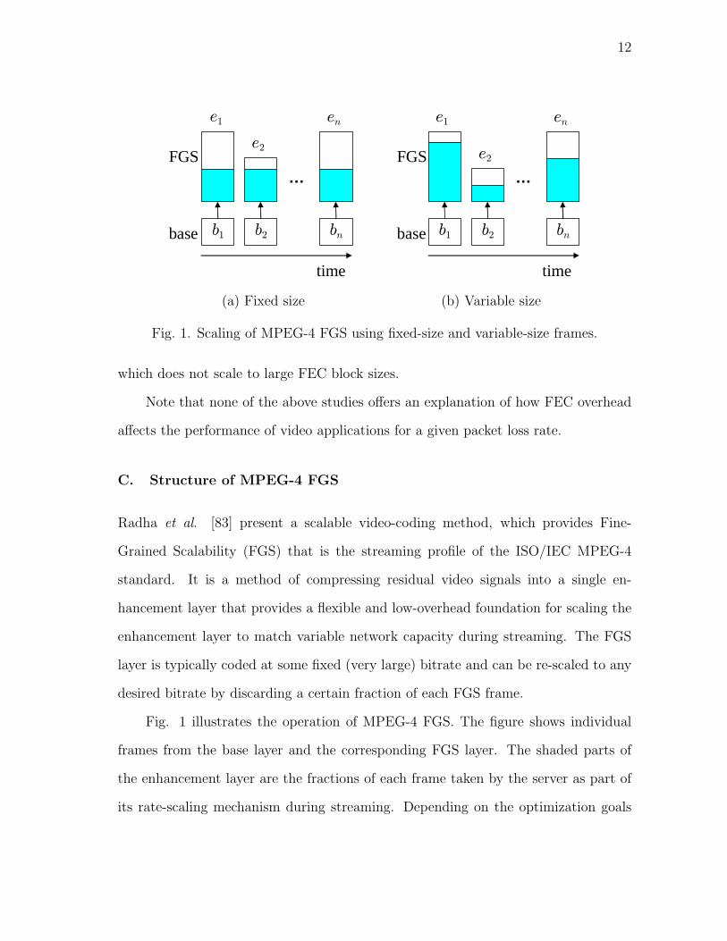
1 Scaling of MPEG-4 FGS using fixed-size and variable-size frames. . . 12

2 The number of useful FGS packets in each frame (left). Utility of

received video (right). . . . . . . . . . . . . . . . . . . . . . . . . . . 28

3 Useful data in each frame under random and ideal loss patterns. . . . 29

4 Router queues for PELS framework. . . . . . . . . . . . . . . . . . . 31

5 Partitioning of the FGS layer into two layers and PELS coloring

of FGS packets. . . . . . . . . . . . . . . . . . . . . . . . . . . . . . . 33

6 Stability of γ with different σ. . . . . . . . . . . . . . . . . . . . . . . 37

7 Simulation topology. . . . . . . . . . . . . . . . . . . . . . . . . . . . 43

8 The evolution of γ (left). The corresponding red loss rates (right). . . 44

9 Green (left) and yellow (right) delays. . . . . . . . . . . . . . . . . . 45

10 Red packet delays in PELS (left). Convergence and fairness of

MKC congestion control (right). . . . . . . . . . . . . . . . . . . . . . 46

11 PSNR of CIF Foreman reconstructed with two different packet

loss p. . . . . . . . . . . . . . . . . . . . . . . . . . . . . . . . . . . . 48

12 Two-state Markov chain. . . . . . . . . . . . . . . . . . . . . . . . . . 53

13 Simulation results of E[ZHj ] and UH for p = 0.1. . . . . . . . . . . . . 56

14 ON/OFF process V (t) (top) and the transmission pattern of video

frames (bottom). . . . . . . . . . . . . . . . . . . . . . . . . . . . . . 59

15 Packet loss patterns for exponential (top) and Pareto (bottom) Yi. . 65

16 Distribution of L(n) for n = 400 and two different p. . . . . . . . . . 73

xiv

FIGURE Page

17 Distribution of L(n) for p = 0.4 (p00 = 0.4, p11 = 0.1). . . . . . . . . 74

18 Distribution of Lc(n) for n = 400 and two different p. . . . . . . . . . 77

19 Simulation results of UH and their comparison to model (87) for

Bernoulli loss and Markov loss (p00 = 0.92, p11 = 0.28). In both

figures, p = 0.1. . . . . . . . . . . . . . . . . . . . . . . . . . . . . . . 83

20 (a) UH computed from (86) for n = 100 and different values of η.

(b) Simulation results of UH for renewal loss. In both figures, p = 0.1. 84

21 ns2 simulation topology. . . . . . . . . . . . . . . . . . . . . . . . . . 88

22 Packet loss pattern obtained through Markov-chain simulation us-

ing transition probabilities p00 and p11. . . . . . . . . . . . . . . . . . 89

23 Metric UH achieved by the adaptive FEC overhead controller (96)

and its comparison to utilities obtained in two different scenarios

that use fixed amounts of overhead. . . . . . . . . . . . . . . . . . . . 90

24 (a) Average packet loss rate for different number of FTP flows N

in ns2 simulation. (b) Packet loss pattern obtained through ns2

simulation. . . . . . . . . . . . . . . . . . . . . . . . . . . . . . . . . 91

25 Evolution of UH achieved by the adaptive FEC overhead con-

troller (96) and its comparison to that of utilities obtained in two

different scenarios that use fixed amounts of overhead. . . . . . . . . 91

26 PSNR of CIF Foreman reconstructed with different FEC overhead

control. . . . . . . . . . . . . . . . . . . . . . . . . . . . . . . . . . . 92

27 Departure delays introduced by the node. . . . . . . . . . . . . . . . 98

28 Single-link simulation topology. . . . . . . . . . . . . . . . . . . . . . 103

29 The histogram of measured inter-arrival times yn under CBR

cross-traffic. . . . . . . . . . . . . . . . . . . . . . . . . . . . . . . . . 104

30 The histogram of measured inter-arrival times yn under TCP

cross-traffic. . . . . . . . . . . . . . . . . . . . . . . . . . . . . . . . . 104

xv

FIGURE Page

31 (a) The absolute error of the packet-pair estimate under TCP

cross-traffic of r = 1 mb/s. (b) Evolution of Wn. . . . . . . . . . . . . 106

32 The histogram of measured inter-arrival times Zkn based on packet

trains and CBR cross-traffic of r = 1.3 mb/s. . . . . . . . . . . . . . 109

33 Evolution of relative estimation errors eC and eA of (123) and

(125) over a single congested link with C = 1.5 mb/s and 85%

link utilization. . . . . . . . . . . . . . . . . . . . . . . . . . . . . . . 115

34 Relative estimation errors eA produced by Spruce and IGI over a

single congested link with C = 1.5 mb/s and 85% link utilization. . . 115

35 Convergence of ωn to zero-mean additive noise for large xn under

CBR and TCP cross-traffic. . . . . . . . . . . . . . . . . . . . . . . . 117

36 A probe-train of m packets that is used for parameter tuning. . . . . 123

37 Simulation topology. . . . . . . . . . . . . . . . . . . . . . . . . . . . 126

38 Evolution of relative available bandwidth estimation error eA of

Spruce for different values of link utilization ρ in case VII. . . . . . . 136


IGI for different values of link utilization ρ. In both cases, the IGI

algorithm stops at E[yi] = 1.1x. . . . . . . . . . . . . . . . . . . . . . 137


IGI for different values of link utilization ρ. In both cases, the IGI

algorithm stops at E[yi] = 1.001x. . . . . . . . . . . . . . . . . . . . 138

41 (a) Relative estimation error eC of CapProbe for different utiliza-

tion ρ of the links in case VII. (b) Evolution of relative capacity

estimation error eC of CapProbe for ρ = 80%. . . . . . . . . . . . . . 140

42 Relative estimation errors eC and eA of Envelope for varying

probe-train length Na in case I under TCP cross-traffic. . . . . . . . 143

43 Relationship between input rate rI and output rate rO. . . . . . . . . 152

44 Probing response curves for different values of probe-train length

N in Emulab experiments. . . . . . . . . . . . . . . . . . . . . . . . . 154

xvi

FIGURE Page

45 Probing response curves for different probe-train length N in ns2

simulation. . . . . . . . . . . . . . . . . . . . . . . . . . . . . . . . . 155

46 Evolution of relative estimation errors eA and eC of PRC-MT for

different N . . . . . . . . . . . . . . . . . . . . . . . . . . . . . . . . . 156

47 Evolution of ratio rI/rO for different values of N . . . . . . . . . . . . 158

48 Evaluation topology in Emulab. . . . . . . . . . . . . . . . . . . . . . 163

49 Convergence characteristics of PRC-MT for cases II and IV. . . . . . 165

50 (a) Relative OWDs obtained using the path configuration in case

I. (b) Remaining OWDs after removing coalesced packets. . . . . . . 171

51 Scale coefficients of wavelet decomposition and window-based av-

erages of one-way delays shown in Fig. 50(a). . . . . . . . . . . . . . 174

1

CHAPTER I

INTRODUCTION

The Internet is a global information infrastructure, which facilitates users to access

information using various networked (inter-connected) systems and applications. Dur-

ing the last decade, it has exhibited an explosive growth of the use of audio and video

content that is provided by a variety of commercial, educational, and individual web-

sites. As a result, real-time streaming that transports multimedia data has become an

important part of the present Internet and attracted significant research effort from

the industry and academic community. However, delivering high-quality of video to

end users over the best-effort Internet is a challenging task since multimedia data is

very sensitive to certain QoS (quality of service) characteristics (such as delay and

packet loss) and quality of streaming video is highly subject to network conditions

that often dynamically change over time. A fundamental issue in this area is how

real-time applications cope with network dynamics (such as variation in delays due

to network queuing and packet loss caused by congestion and/or other reasons) and

adapt their operational behavior to offer a high-quality streaming environment to end

users.

A. Objective and Approach

To address this issue, one dimension of work focuses on improving the best-effort

model of the current Internet [9], [15], [19], [25], [29], [91] by supplementing it with

The journal model is IEEE/ACM Transactions on Networking.

2

some form of network QoS. These methods include DiffServ (Differentiated Services)

[9], [15] and IntServ (Integrated Services) [12] proposals and various Active Queue

Management (AQM) algorithms [19], [25], [29], [57], [91], offering prioritized services

to different flows. The other dimension of related work is based on end-to-end methods

that depend solely on end-system entities without network support and are associated

with end-to-end rate and error control [7], [79], [103].

Although existing studies report certain success in improving the video stream-

ing quality, none of them is sufficient to support a scalable, low-overhead, low-delay,

and retransmission-free platform required by many current real-time streaming ap-

plications since they are not able to effectively utilize video-specific features such

as unequal importance of multimedia packets, time limits in decoding of received

packets, and an impact of packet loss on scalable video.

As an effort towards providing a high-quality scalable streaming environment

that is free of retransmission, we investigate AQM-enabled schemes that can effec-

tively utilize different importance of video packets and provide QoS services to flows

with much less overhead than the mechanisms like DiffServ or IntServ. To understand

and quantify how packet loss affects quality of scalable video, we analyze the perfor-

mance of video streaming in best-effort networks. Based on this analysis, we propose

a new streaming framework that allows applications to mark their own packets with

different priorities and uses AQM inside routers to effectively drop less-important

packets during buffer overflows. This framework achieves “optimal” transmission

of video packets for a given packet loss rate without recovering packets lost during

congestion.

Different from the above method, many real-time applications employ error con-

cealment techniques to recover packets lost during transmission without retransmit-

ting them. Forward-Error Correction (FEC) is widely used in streaming applications

3

to protect audio and video data in lossy network paths, which provides retransmission-

free network services. However, it requires to send additional information with the

data, which is in general not desirable for applications because of additional band-

width requirements. FEC is seemingly beneficial for streaming services, but is not

well understood how inclusion of redundant FEC packets affects the performance of

scalable video and its resilience characteristics for a given packet loss rate. Thus,

we examine FEC-protected transmission of video data and study the effect of packet

loss within an FEC block and derive the asymptotic (i.e., assuming large sending

rates) distribution of the number of lost packets per FEC block, which enables us to

model the performance of video streaming with FEC protection. This result reveals

a relationship between the FEC overhead rate and the end-to-end utility of received

video and leads to optimal selection of FEC rate for a given packet loss rate and FEC

block size.

In the second part of this thesis, we focus on measuring characteristics of network

paths, which can be utilized by rate control algorithms for real-time traffic. Note that

it is often believed that rate control is necessary for streaming applications to provide

a high level of video quality to end users and avoid wasting network resources with

packets that are eventually dropped in congested routers. With the development of

scalable video such as MPEG-4 Fine Granular Scalability (FGS) [83], real-time video

applications can implement rate control that re-scales the enhancement layer of the

video stream to any desired bit rate. However, typical end-to-end congestion control

mechanisms in the best-effort network rely on packet loss to probe for available band-

width, which may cast a serious challenge to real-time flows because lost packets may

need to be recovered before their decoding deadlines. This packet loss problem can

be significantly improved by supplementing rate control mechanisms with bandwidth

information discovered by other tools [64].

4

Given the importance of this topic and lack of stochastic analysis of this problem,

we study packet-pair/train sampling techniques that have been used in the majority

of existing bandwidth estimators and develop a generic queuing model of an Internet

router. We then stochastically analyze bandwidth sampling process in the context

of a single-congested node under non-negligible, non-stationary, and non-fluid cross-

traffic conditions and derive an asymptotically accurate bandwidth estimator for both

capacity and available bandwidth. This is one of the first methods that simultaneously

estimates both types of bandwidth and is provably accurate. Following the single-hop

analysis, we focus on developing an automated tool that measures both bandwidth

metrics of a multi-hop path with asymptotic accuracy by utilizing recursive extension

of the single-hop model. This automated tool relies on hop-by-hop measurement and

adaptively selects probing parameters according to network conditions.

Finally, we note that all existing bandwidth estimation methods heavily rely on

high-precision packet timing at measurement hosts. However, timing irregularities

caused by OS (Operating System) scheduling jitter and hardware interrupt modera-

tion are common in real networks, in which certain algorithms (e.g., [44]) reveal severe

performance issues. On the other hand, theoretical models (e.g., [48], [61], [69], [75])

usually have probable convergence, but not have practical implementation to become

a measurement tool. To address these issues related to realistic measurement envi-

ronment, we develop a measurement tool PRC Measurement Tool (PRC-MT) based

on asymptotically accurate bandwidth models of [61] and perform comparative study

of existing tools in non-simulated networks.

B. Contributions

This work makes the following contributions:

5

• A better understanding of how packet loss affects the performance of scalable

video in best-effort networks. We thoroughly study the effect of packet loss on

quality of video under various network conditions. We define quality measure

U , which is the percentage of received data in each frame that can be used for

decoding the frame, and derive closed-form models of U under several general

patterns of packet loss. These analytical results provide statistical insight into

understanding the penalty inflicted on scalable code.

• A new streaming framework that can provide QoS services to real-time flows.

This framework effectively utilizes unequal importance of video packets in rate

control and achieves a near-optimal performance for a given network packet loss

rate without recovering packets lost during transmission.

• A new performance measure of the quality of scalable video with FEC protec-

tion and its resilience characteristics and a new method of optimally selecting

FEC overhead rate for a given network packet loss rate. As an alternative to

retransmission-based error recovery, we investigate error concealment methods

such as FEC, which is often used to protect multimedia data over lossy net-

work channels. In FEC-protected video, the distribution of the number of lost

packets and the location of the first loss in a block play an important role in

understanding the effectiveness of FEC. Thus, we first study these two met-

rics and derive a model for each assuming large sending rates. Based on these

results, we then develop models that enable us to understand optimality and

resilience characteristics of scalable video under dynamically changing network

conditions.

• New bandwidth sampling techniques and measurement tools. We study the prob-

lem of estimating bandwidth of network paths. First, we build a generic stochas-

6

tic queuing model of an end-to-end path and develop a new bandwidth sampling

method in the context of a single-congested node, which can produce asymp-

totically accurate capacity and available bandwidth estimates of network paths

under non-negligible and arbitrary cross-traffic. We next apply recursive exten-

sion of this single-hop model to a multi-hop path and develop an automated

measurement tool that measures tight-link of the path by hop-by-hop probing.

In addition, we develop a new measurement tool called PRC-MT based on theo-

retical models of [61] and conduct a comparative study of existing measurement

tools in non-simulated networks where delay measurement is not accurate due to

various timing irregularities. This study shows that PRC-MT significantly out-

performs existing tools and reveals performance issues of certain algorithms such

as Pathload when end-hosts delay generation of interrupts for network hardware.

We overcome this timing problem by incorporating signal de-noising techniques

into bandwidth measurement and develop a measurement tool called Interrupt

Moderation Resilient Pathload (IMRP) that significantly improves Pathload’s

estimation reliability under a wide range of interrupt delays.

C. Dissertation Organization

The rest of the dissertation is organized as follows. In Chapter II, we describe back-

ground and related work of this thesis. Chapter III analyzes performance of scalable

video streaming in best-effort networks and introduces a new streaming framework

based on AQM. In Chapter IV, we examine performance of streaming video under

FEC protection and discuss its optimality and resilience characteristics. Chapter V

presents a stochastic analysis of bandwidth estimation in the context of a single-

congested node and its extension to multi-hop paths, while in Chapter VI, we in-

7

vestigate practical issues of bandwidth measurement in real networks where delay

measurements are not perfect due to hardware-related timing irregularity. Finally,

we conclude this work and discuss future directions in Chapter VII.

8

CHAPTER II

BACKGROUND AND RELATED WORK

In this chapter, we review prior work in the areas of Internet QoS, error control, and

bandwidth estimation.

A. Internet QoS Studies

Studies in this area supplement the best-effort model of the current Internet to provide

a “better than best-effort” performance to end flows. Some of them focus on AQM

(Active Queue Management) [19], [25], [29], [91] that provides unequal treatment to

flows while controlling congestion and achieving fairness among the flows. Other work

ranges from offering hard guarantees in the form of Integrated Services (IntServ) [12],

[88], [106] to more scalable models such as Differentiated Services (DiffServ) [9], [15].

We overview some of these approaches that are related to the following two categories.

1. Priority QoS Methods

Several studies investigate the performance of video streaming over the DiffServ ar-

chitecture. Gurses et al. [33] study streaming of temporally-scalable H.263+ video

over a DiffServ network and propose three-color markers (TCM), which allow ingress

routers to promote packets (i.e., increase their priority) or demote them based on

their conformity to agreement between peering ISPs. Although this work provides

flow differentiation at routers, it does not allow the end flows to effectively bene-

fit from unequal priority of the packets since DiffServ can arbitrarily remark them

according to ingress/egress policies of peering ISPs.

9

Shin et al. [89], [90] study the problem of “optimal” assignment of relative

priority indexes to video packets depending on their impact on the quality of received

video. Besides using a fairly complex packet prioritization scheme, the work does

not discuss how the network should treat marked packets. Zhao et al. [108] employ

MPEG-4 FGS for video streaming and use several computationally intensive packet

prioritization schemes, but also without studying network support of the proposed

architecture.

Among non-DiffServ methods, Tang et al. [98] present a rate control scheme

called RCS for real-time traffic, which uses low-priority dummy packets to probe for

new bandwidth at the beginning of a new connection and upon detection of data

packet loss. When a new connection is started, the RCS source sends dummy packets

with a predefined rate that can support for the highest quality of encoded video

for the duration of one round-trip time (RTT). If the source detects loss of data

packets at a current sending rate R of data packets, it sends dummy packets with the

current sending rate R for one RTT. This method assumes priority queuing policies

at intermediate routers on an end-to-end path to drop the dummy packets first during

congestion.

Hurley et al. [38] propose ABE (Alternative Best Effort), which allows applica-

tions to choose between two types of service by marking their own packets as either

green for low delay or blue for low packet loss based on the nature of their traffic.

All green packets are served at each router within a certain predefined delay or oth-

erwise dropped, while blue packets do not get special treatment from the routers.

A similar approach is used in BEDS (Best Effort Differentiated Service) [26], which

distinguishes two service classes similar to ABE using two RED (Random Early De-

tection) queues. BEDS employs small queue and aggressive RED drop probability

and thresholds for low-latency service. On the other hand, it uses large queue and

10

less aggressive drop probability and thresholds for low-loss service.

Internet-2’s QBSS (QBone Scavenger Service) [82] also provides service differ-

entiation by allowing end flows to mark their own packets with the low-priority bit.

However, the current QBSS does not support more than two priorities or directly ben-

efit video traffic. Similarly, Li et al. [59] also suggests flow differentiation based on

priorities assigned by applications, but without offering how real-time applications

use different priorities in conjunction with rate control to improve their streaming

quality.

2. Active Queue Management

Active Queue Management (AQM) schemes perform special operations in the router

to achieve better performance for end flows. These operations include dropping ran-

dom packets (e.g., RED), re-arranging the order in which packets are served (e.g.,

WFQ (Waited Fair Queuing)), and randomly marking packets from more aggressive

flows (e.g., ECN (Explicit Congestion Notification)). While WFQ focuses on provid-

ing fairness to competing flows [19], [91], RED/ECN attempt to avoid congestion by

randomly dropping or marking packets with a certain probability that increases with

the level of congestion [25], [27], [29]. As such, these methods are not specifically tai-

lored to multimedia applications and thus cannot significantly improve video quality

of Internet streaming.

Additional studies combine congestion control with AQM to provide robust and

smooth controllers since routers can detect network conditions more accurately than

end systems. Lapsley et al. [57] study optimization-based congestion control and

propose REM (random early marking) that carries congestion information using ex-

ponential marking based on user’s utility. Katabi et al. [50] present XCP (eXplicit

Congestion notification Protocol) that conveys information about the degree of con-

11

gestion in network paths to application sources using separate AQM controllers for

utilization and fairness. Several other studies include Kelly-style optimization frame-

work [46], [51], [53], [71] and Low’s work [65], [66], [67], [68]. Note that none of those

methods are coupled with multimedia streaming.

B. Forward Error Correction

FEC methods can recover lost data segments using extra information transmitted to-

gether with the data. We discuss some of the studies that report somewhat conflicting

results on the benefits of FEC.

Altman et al. [3] study simple media-specific FEC for audio transmission and

show that it provides little improvement to the quality of audio under any amount of

FEC. This work uses media-specific FEC that is sometimes less effective in recovering

lost packets than media-independent FEC [79]. Biersack et al. [7] evaluate the effect

of FEC for different traffic scenarios in an ATM network. This study measures the

reduction of loss rate for each source and reports that the performance gain of FEC

quickly diminishes when all traffic sources employ FEC and the number of sources

increases.

Alternative approaches aim to maximize the effect of FEC by choosing the proper

amount of overhead and avoiding unlimited rate increase by keeping the combined rate

R + F (where R is the streaming rate of the application and F is the FEC overhead

rate) equal to some constant S. Bolot et al. [11] present a media-specific method for

adjusting FEC overhead under certain constraints on the total sending rate S. That

work achieves close to optimal audio-specific subjective quality. Frossard et al. [31]

propose a method that selects rates R and F using the distortion perceived by end-

users. The method is fairly complex since it involves solving recurrence equations,

12

b1 b2

e2

bn

en

…

base

FGS

e1

time

(a) Fixed size

b1

e1

b2

e2

bn

en

…

base

FGS

time

(b) Variable size

Fig. 1. Scaling of MPEG-4 FGS using fixed-size and variable-size frames.

which does not scale to large FEC block sizes.

Note that none of the above studies offers an explanation of how FEC overhead

affects the performance of video applications for a given packet loss rate.

C. Structure of MPEG-4 FGS

Radha et al. [83] present a scalable video-coding method, which provides Fine-

Grained Scalability (FGS) that is the streaming profile of the ISO/IEC MPEG-4

standard. It is a method of compressing residual video signals into a single en-

hancement layer that provides a flexible and low-overhead foundation for scaling the

enhancement layer to match variable network capacity during streaming. The FGS

layer is typically coded at some fixed (very large) bitrate and can be re-scaled to any

desired bitrate by discarding a certain fraction of each FGS frame.

Fig. 1 illustrates the operation of MPEG-4 FGS. The figure shows individual

frames from the base layer and the corresponding FGS layer. The shaded parts of

the enhancement layer are the fractions of each frame taken by the server as part of

its rate-scaling mechanism during streaming. Depending on the optimization goals

13

of the server, it can transmit a fixed fraction of each frame or use rate-distortion

(R-D) models to dynamically determine the desired amount of data in each frame

(interested readers are referred to [17] for more details).

D. Bandwidth Estimation

There are two types of bandwidth metrics: bottleneck bandwidth and available band-

width. The former is the capacity of the slowest link (often called the narrow link) of

an end-to-end path, while the latter represents the smallest unused bandwidth of links

in the path. The link with the smallest unused bandwidth is referred to as the tight

link. We discuss some of bandwidth estimation techniques that have been proposed

in the literature separately below, starting with bottleneck-capacity estimators.

1. Capacity Measurement

Transmission delay of a packet over a link is solely determined by the capacity of the

link and the size of the packet. Hence, capacity measurement techniques based on

active probing focus on identifying transmission delay of probe packets that are sent

over a link under investigation.

One of the earliest such tools is Pathchar [41], which is developed by Van Jacob-

son in 1997 and infers characteristics (such as capacity, latencies, and queuing delays)

of individual links along an Internet path by exploiting the TTL field of IP packets.

To probe each router, Pathchar sends multiple packets per packet size arranged in a

linearly increasing order and drops them in a select router by TTL-limiting. Each

of the ICMP error messages returned by a router due to TTL-expiration provides

an estimate of round-trip time to that particular router. Recognizing the effect of

cross-traffic on the measured RTT, Jacobson employs minimum filtering to keep the

14

minimum RTT sample per packet size. Capacity of each link can be estimated using

the linearly increasing slope of the minimum RTTs as a function of probe-packet size.

More recent work exploits inter-packet dispersions (delays) sampled at the re-

ceiver to estimate the narrow-link capacity of a path rather than individual link

capacities. The main idea is based upon an observation by Jacobson [42] in 1988 that

the inter-arrival dispersion of two back-to-back packets (a packet-pair) injected into

an idling network represents transmission delay of the second packet in the packet-

pair over the narrow link. However, in real networks, inter-packet dispersions exiting

from the narrow-link router will be distorted by cross-traffic at routers on the path.

Specifically, if cross-traffic delays the first packet in the probing pair, the dispersion

is compressed, while it is expanded when cross-traffic queues between the two prob-

ing packets. This variation (noise) in output dispersion due to random queueing of

probe packets at intermediate routers is the primary source of error in bandwidth

measurement. Thus, the majority of work in this area centers around how to filter

out random queuing effects embedded in the measured output dispersions.

In order to facilitate removal of random noise in the output dispersion samples,

several studies investigate different filtering techniques. Carter et al. [14] propose

bprobe that sends a sequence of ICMP echo packets and measures inter-arrival times

of returning successive packets. In this approach, the source sends a series of n = 10

packets of size qi for each phase φi (where i = 1, 2, . . . , 7 and qi < qj if i < j). In

each phase φi, the source computes a capacity range [Ck,i, Ck,i + ε] for each estimate

Ck,i = qi/yk between two consecutively returning packets k and k + 1, where yk is

the inter-arrival delay between returning packets k and k + 1 and ε is a certain small

constant. Then, bprobe selects the most overlapping capacity range by iteratively

intersecting the capacity ranges obtained in prior phases (starting from the last phase

that uses the largest packet size) and produces a capacity estimate as the middle

15

point of the most overlapping capacity range. Other similar methods that use the

most common output dispersion to estimate the capacity includes Nettimer [54] and

PBM [78].

Recently, Dovrolis et al. [21] study characteristics of bandwidth estimation tech-

niques that use packet-trains (packet-pairs are a special case of packet trains with

train length N = 2) and model intermediate routers assuming a continuous fluid

approximation for cross-traffic. This work shows that packet-pair histograms usually

have many different modes (also observed in [78]) and that packet-train histograms

become unimodal as the length N of packet-trains increases. This work also re-

ports that the unique mode is centered at ADR (Asymptotic Dispersion Rate) that

is lower than the capacity of the path. Based on this observation, the paper pro-

poses a capacity estimator called Pathrate that uses two-phase probing and relies on

histogram-based heuristics for actual bandwidth estimation. The two-phase probing

methodology attempts to discover all local modes in the first phase by sending a

large number of packet-pairs and continues the second phase unless the histogram of

packet-pair samples is unimodal (which can happen in very lightly loaded paths).

In the second phase, Pathrate sends packet trains with length N > 2. If the

resulting dispersions of packet train samples are not unimodal, then the probing

source increases the train length N by a factor of 2 and repeats the process. When

the resulting dispersions become unimodal, Pathrate’s internal algorithm heuristically

determines a range [ζ−, ζ+] of the unique mode centered at ADR and selects, as the

capacity estimate C, the minimum local mode mk that is higher than ζ+ from a

sequence of local modes M = {m1,m2, . . . , mM} obtained in the first phase:

C = mk = min(mi ∈ M : mi > ζ+). (1)

This heuristic rule in (1) is based on the assumption that ζ+ < C and the range of

16

the unique mode [ζ−, ζ+] covers all the local modes between ADR and C.

In addition to histogram-based proposals, other methods include packet tailgat-

ing [55], where larger packets are followed by smaller packets to ensure a particular

queuing pattern at the narrow link, and packet cartouche [35], where certain packets

in a probe-train are dropped at select routers (using the TTL field) so as to ensure

that the surviving packets can measure the capacity of individual routers and/or

subpaths.

Besides the methods discussed above, a recent approach called CapProbe [49] is

based on the assumption that if packets in a probe pair have arrived at the receiver

with the smallest combined one-way delay, then the packets have not been queued at

any intermediate routers in the path and thus the inter-packet delay of the probe pair

reflects the transmission delay of the bottleneck link. Based on this assumption, Cap-

Probe sends up to 100 packet-pairs and finds a minimum-delayed pair that satisfies

the following condition:

mini

(d1,i + d2,i) = mini

(d1,i) + mini

(d2,i), (2)

where i represents packet-pair sequence number and d1,i and d2,i are the respective

one-way delays of the first and second packets in i-th packet-pair. If such a minimum

delay pair satisfying the above condition is not found from 100 probe samples, then

CapProbe adjusts the size of probe-packets and repeat this process. Using minimum

filtering, CapProbe is frequently able to obtain C with better accuracy and much

quicker than the previous methods.

2. Available Bandwidth Measurement

Unlike link capacity, available bandwidth is an elastic metric that varies over time

depending on the amount of cross-traffic on a network path. Research in this area

17

focuses on statistical nature of output inter-packet dispersions that reflect dynamics

of cross-traffic through the path. Based on the analysis of dispersion information,

various techniques have been proposed. One of the earliest approaches, called cprobe

[14], directly relates the average of inter-arrival packet dispersions to the available

bandwidth estimate A by dividing the probe packet size by the average dispersion.

Subsequent more sophisticated approaches (such as [37], [44], [72], [85], [96]) center

around discovering a relationship between the input and output dispersions and how

to utilize this relationship in actual measurement of the path.

Melander et al. [72] study the dependency between input rate RI and output

rate RO of probe packets and derive the following expression for a single-link path

under a fluid assumption on cross-traffic:

RO =

RI RI < A

RI

RI + λC RI ≥ A

, (3)

where C and A are the capacity and available bandwidth of the path, respectively.

Based on this single-link model, this work proposes a new bandwidth probing tech-

nique called TOPP (Trains of Packet Pairs), which sends a sequence of packet-pair

trains with increasing rates in subsequent trains. The input rates of probe-pair trains

are selected in a predefined range and average output rates of each train are collected

for further analysis. Re-writing (3), the paper obtains a linear relationship between

two metrics RI/RO and RI :

RI

RO

=

1 RI < A

RI

C+

λ

CRI ≥ A

. (4)

Then, TOPP extracts from (4) both C and λ by exploiting the linear relationship

between RI/RO and RI using the collected average output rates and thus obtains

18

A = C−λ. In the multi-hop case, the paper reports that (4) can extract A assuming

that available bandwidth of the second tight-link following the tight-link is obtained

using empirical methods.

Different from TOPP, Pathload proposed by Jain et al. [44] adjusts input rates

of packet-trains to infer available bandwidth of the path. This work is based on an

observation that if the input probe rate is higher than the available bandwidth of

the path, then one-way delays of packets in a probing-train exhibit an increasing

trend. Pathload sends a fleet of n packet-trains, each of which consists of N back-

to-back packets with inter-packet spacing x. After all packets in a train are received,

the receiver performs a trend test on one-way delays of packets in the train. For the

trend test, Pathload uses simple methods called Pairwise Comparison Test (PCT) and

Pairwise Difference Test (PDT). The PCT metric represents how often consecutive

one-way delays in a probe-train increase, while PDT metric quantifies how strong the

difference between the first and last one-way delays in the data set is. After receiving

all packets in n trains, the receiver determines the trend of the fleet based on the

fraction of n trains that is of increasing or no-trend. When the trend information for

a fleet is fed back to the source by the receiver, Pathload searches for an available

bandwidth region by increasing or decreasing the input probing rate at the sender in

a binary search fashion based on the trend information.

Another recent approach that is based on the one-way delay variation is Pathchirp

[85], which focuses on reducing the measurement overhead of Pathload. In [85],

Pathchirp uses packet-trains (called chirps) with exponentially decreasing inter-packet

spacings and infers available bandwidth using the queuing delay signature of arriving

chirps. The basic idea behind this method is that when a transmission rate rk = q/xk

of a packet k in the train reaches the available bandwidth of the path, then subsequent

packets j > k in the chirp will exhibit increasing queueing delay. Hence, the available

19

bandwidth of the path is the rate rk of the packet at which the queueing delay starts

increasing.

Considering bursty cross-traffic and non-monotonic increase of queueing delays,

Pathchirp employs an empirical method to detect and interpret different patterns of

queueing delay variations of probe packets in a packet-train. In reality, Pathchirp uses

one-way delays in place of queuing delays since the latter is not easily measurable.

It then classifies these delays into three groups based on variations of successive one-

way delays and infers per-packet available bandwidth using heuristics, which leads

to per-train available bandwidth after averaging the per-packet available bandwidth

over the duration of that train.

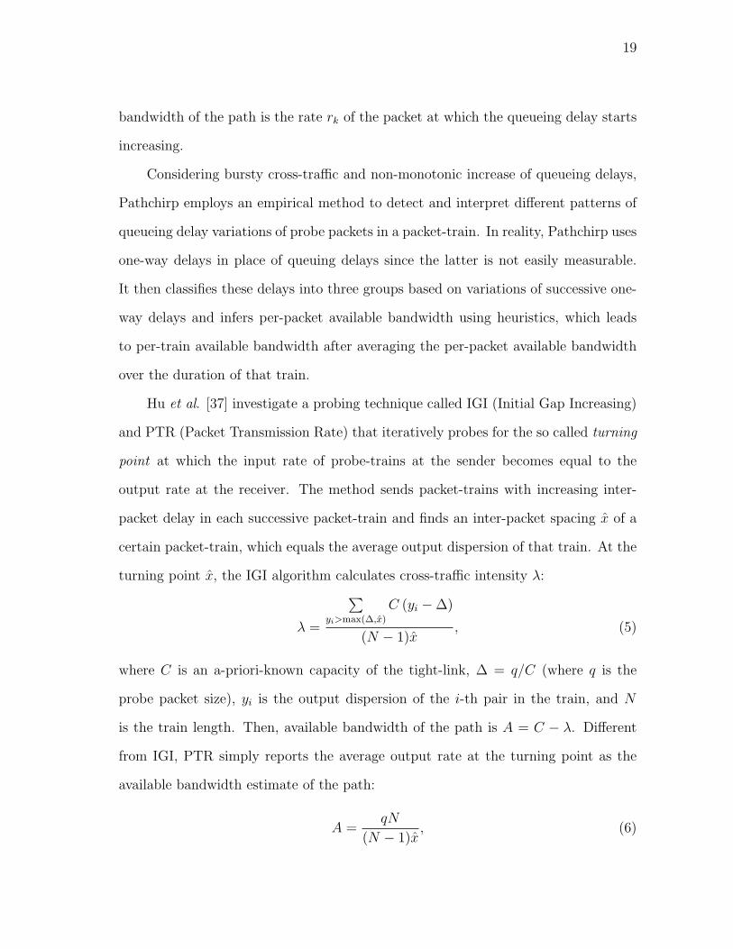
Hu et al. [37] investigate a probing technique called IGI (Initial Gap Increasing)

and PTR (Packet Transmission Rate) that iteratively probes for the so called turning

point at which the input rate of probe-trains at the sender becomes equal to the

output rate at the receiver. The method sends packet-trains with increasing inter-

packet delay in each successive packet-train and finds an inter-packet spacing x of a

certain packet-train, which equals the average output dispersion of that train. At the

turning point x, the IGI algorithm calculates cross-traffic intensity λ:

λ =

∑yi>max(∆,x)

C (yi −∆)

(N − 1)x, (5)

where C is an a-priori-known capacity of the tight-link, ∆ = q/C (where q is the

probe packet size), yi is the output dispersion of the i-th pair in the train, and N

is the train length. Then, available bandwidth of the path is A = C − λ. Different

from IGI, PTR simply reports the average output rate at the turning point as the

available bandwidth estimate of the path:

A =qN

(N − 1)x, (6)

20

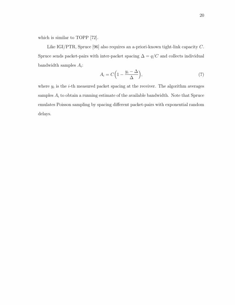
which is similar to TOPP [72].

Like IGI/PTR, Spruce [96] also requires an a-priori-known tight-link capacity C.

Spruce sends packet-pairs with inter-packet spacing ∆ = q/C and collects individual

bandwidth samples Ai:

Ai = C(1− yi −∆

∆

), (7)

where yi is the i-th measured packet spacing at the receiver. The algorithm averages

samples Ai to obtain a running estimate of the available bandwidth. Note that Spruce

emulates Poisson sampling by spacing different packet-pairs with exponential random

delays.

21

CHAPTER III

MULTI-LAYER ACTIVE QUEUE MANAGEMENT

FOR SCALABLE VIDEO STREAMING

In this chapter, we study video streaming over best-effort networks and analyze per-

formance characteristics of scalable video under uniformly-random packet loss using

MPEG-4 FGS as the example scalable video. Quantifying drastic quality degradation

of streaming video in best-effort networks, we propose a new streaming framework

that allows applications to mark their own packets with different priority and use

multi-queue congestion control inside routers to effectively drop the less-important

packets during buffer overflows. We describe priority AQM algorithms that provide

“optimal” performance to video applications under arbitrary network loss and study

a variation of Kelly’s congestion control in combination with our framework.

A. Introduction

Typical video applications transport multimedia data that is highly sensitive to

quality-of-service (QoS) characteristics (e.g., delay or packet loss) of their end-to-

end path and often require better than simply best-effort services from the network

before they can offer a high-quality streaming environment to end users. In response

to this demand, significant research effort went into improving the best-effort model

of the current Internet [9], [15], [19] , [25], [29], [91].

One dimension of this related work supplements the best-effort model with net-

work QoS that guarantees a “better than best-effort” performance to end flows (these

methods loosely fall under the umbrella of DiffServ [9], [15]). The other, more recent

22

dimension includes various Active Queue Management (AQM) algorithms [19], [25],

[27], [29], [57], [91] that are able to provide QoS services to the flows with much less

overhead than the more traditional mechanisms like DiffServ or IntServ [12].

However, none of the existing QoS methods provide a scalable, low-overhead, low-

delay, and retransmission-free platform required by many current real-time streaming

applications. To fill this void, we investigate novel AQM algorithms that not only

can provide a provably “optimal” performance under random loss, but also possess

very low implementation complexity.

One of the characteristics of video packets that does not match the best-effort

service is that they often carry information of different importance. Thus, video appli-

cations can clearly differentiate between the more-important and the less-important

packets. In all layered video coding schemes, the base layer is more important than

the enhancement layer. Furthermore, the lower sections of the enhancement layer are

more important than the higher sections because their loss renders all dependent data

virtually useless. Thus, treating all video packets equally (as in the current best-effort

Internet) usually leads to significant quality degradation during packet loss and low

useful throughput during congestion, both of which cause video streaming to become

unappealing in practical settings.

With the presence of unequal importance among video packets, the first goal

of this work is to achieve “high end-user utility,” which means that the majority of

packets that are transmitted across the bottleneck link must carry useful information

that can be decoded by the receiver. In video applications that use motion compen-

sation and variable-length coding (VLC), a single lost packet in the base layer may

affect several frames and render them all useless even though some of them arrive to

the receiver without any loss. Furthermore, the enhancement layer is not immune to

packet loss either since strong dependence between the coded data allows packet loss

23

to affect consecutive chunks of data that are significantly larger than those actually

lost in the network. Hence, even under moderate packet loss, the bottleneck link may

be used to transmit a large number of packets that eventually get dropped by the

decoder.

In addition to high utility, many interactive applications (such as video tele-

phony) further require low end-to-end delays to deliver high application-layer per-

formance to the user. Additional problems with delays arise during retransmission

of lost packets since all video frames have strict decoding deadlines. During heavy

congestion (especially along paths with large buffers), the RTT is often so high that

even the retransmitted packets are dropped in the same congested queues [64]. As

a result, the receiver in such scenarios must ask for multiple retransmissions of each

lost packet, which often causes the retransmitted packets to miss their decoding dead-

lines. Thus, our second goal is to provide a retransmission-free network service to

video flows. This direction generally aligns well with FEC-based approaches, except

our goal is to avoid all bandwidth overhead associated with error-correcting codes

and occupy network channels only with the actual video data.

To improve the quality of video delivered over the Internet, we investigate a new

streaming framework in which each application marks its own packets with different

priorities and uses AQM inside routers to effectively drop the less-important packets

during congestion. Such preferential (instead of random) dropping of packets allows

the application to maintain a much higher quality of video for the end user compared

to similar scenarios in a best-effort network. We also find that the use of multi-

queue AQM allows scalable video applications to maintain high useful link utilization

without retransmitting any of the lost packets or sending any error-correcting codes.

Thus, we achieve both goals of high utility and low end-to-end delay.

While our implementation relies on Kelly’s utility-based controllers [51], it is

24

important to realize that the proposed framework can be used with any congestion

control (including end-to-end methods such as AIMD, TFRC, or even TCP) and

can be deployed in the current Internet with minimum modifications to the existing

infrastructure.

B. Analysis of Video Streaming

In the first part of this section, we investigate probabilistic characteristics of video

streaming performance under random packet loss. We study a best-effort network, in

which routers drop video packets uniformly and randomly during congestion. Recall

that many studies of Internet QoS attempt to improve TCP performance by changing

drop behavior of the network from bursty to uniformly random [27], [29]. Thus, it

can be argued that future networks will deploy such packet drop mechanisms more

often than the current Internet. Therefore, we assume an independent loss model

with exponential tails of burst-length distributions (rather than a heavy-tailed model,

which is commonly observed in FIFO queues) and use it throughout this chapter.

In the second part of this section, we overcome the drastic reduction of video

quality in best-effort streaming and show that preferential packet drops can in fact

provide “optimal” performance to the end-user. Thus, following the best-effort anal-

ysis, we study priority-based AQM that supports preferential streaming and compare

it with the best-effort scheme.

Finally, we should note that although quality degradation of multimedia stream-

ing in best-effort networks is well documented, the novelty of this section lies in the

derivation of the exact closed-form expressions for the penalty inflicted on scalable

flows under uniform packet loss and the novel associated discussion that is also useful

for understanding “optimality” of AQM in later sections.

25

1. Best-Effort Streaming

We investigate the effect of random packet drops on video quality using the example

of MPEG-4 FGS (similar results apply to non-FGS layered coding)1. We start by

examining the probabilistic characteristics of packet drops in an FGS frame, derive the

expected amount of useful data recovered from each frame, and define the effectiveness

of FGS transmission over a lossy channel.

Assume that long-term network packet loss p can be modeled by a sequence of

independent Bernoulli random variables Xi. Each Xi is an indicator function that

determines whether packet i is lost or not: Xi = 1 iff packet i is dropped in the

network. Then P (Xi = 1) = 1 − P (Xi = 0) = E[Xi] = p is the average packet loss.

Even though this model is a great simplification of real networks and results in the

probability of obtaining a burst of length k proportional to e−k (i.e., the tail of burst

sizes is exponential), it suffices for our purposes (see the discussion on RED/ECN

([27], [29]) earlier in this section).

Next assume that FGS frame sizes Hj are measured in packets and are given by

i.i.d. random variables with a probability mass function (PMF) qj = P (Hj = k), k =

1, 2, . . .. The exact distribution of {Hj} depends on the frame rate, variation in scene

complexity, and the bitrate of the sequence. The question we address next is what is

the expected amount of useful packets that the receiver can decode from each frame

under p–percent random loss? Thus, our goal is to determine the expectation of Yj,

which is the number of consecutively received packets in a frame j.

Lemma 1. Assuming independent Bernoulli packet loss with probability p, the ex-

1Further note that motion-compensated enhancement layers suffer even moredegradations under best-effort loss and are not modeled in this work. However, theexpected amount of improvement from QoS in such schemes is even higher than thatin FGS.

26

pected number of useful packets in an FGS frame is:

E[Yj] =1− p

p

∞∑

k=1

(1− (1− p)k

)qk. (8)

Proof. Assume that Gj is the random distance from the beginning of frame j to the

next packet-loss event. Then, all Gj are geometric random variables with respect to

each frame j and can assume any integer value in the range [1,∞). Note that when

the first packet-loss location Gj is no more than Hj, the decoder recovers exactly

Gj − 1 packets from the frame. Otherwise, all Hj packets are recovered.

Next, taking a conditional expectation of Zj, we can write:

E[Yj|Hj = k] =k∑

i=1

(i− 1)pi +∞∑

i=k+1

kpi, (9)

where pi = P (Gj = i) = qi−1p is the geometric PMF of Gj and q = 1− p. Then, (9)

becomes:

E[Yj|Hj = k] = p

k∑i=1

(i− 1)qi−1 + k

∞∑

i=k+1

qi−1p

= p

k∑i=1

(i− 1)qi−1 + k(1− p

k∑i=1

qi−1). (10)

Substituting l = i− 1 into (10), we get:

E[Yj|Hj = k] = p

k∑i=1

lql + k(1− p

k−1∑

l=0

ql)

= pq

k−1∑

l=0

d

dqql + k

(1− p

1− qk

1− q

)=

1− p

p

(1− (1− p)k

). (11)

Expanding the conditional expectation in (11) to arbitrary frame sizes Hj, we

obtain (8).

Throughout the rest of the chapter, we examine one particular distribution of

27

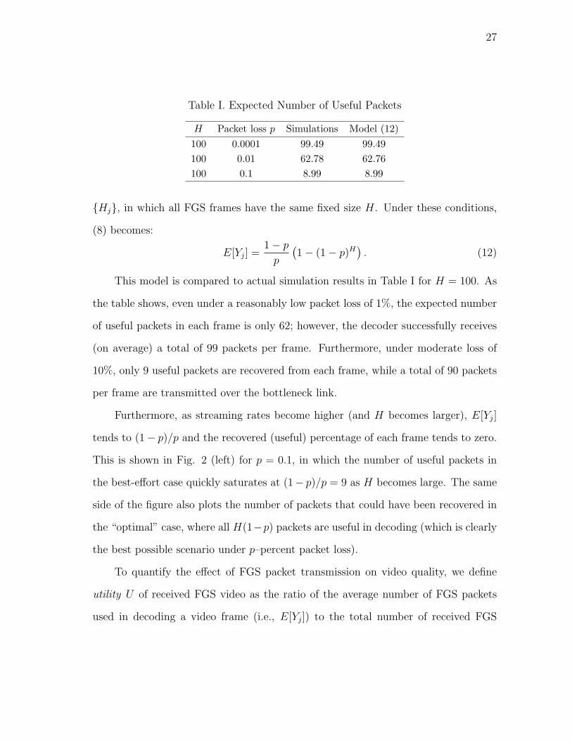
Table I. Expected Number of Useful Packets

H Packet loss p Simulations Model (12)100 0.0001 99.49 99.49100 0.01 62.78 62.76100 0.1 8.99 8.99

{Hj}, in which all FGS frames have the same fixed size H. Under these conditions,

(8) becomes:

E[Yj] =1− p

p

(1− (1− p)H

). (12)

This model is compared to actual simulation results in Table I for H = 100. As

the table shows, even under a reasonably low packet loss of 1%, the expected number

of useful packets in each frame is only 62; however, the decoder successfully receives

(on average) a total of 99 packets per frame. Furthermore, under moderate loss of

10%, only 9 useful packets are recovered from each frame, while a total of 90 packets

per frame are transmitted over the bottleneck link.

Furthermore, as streaming rates become higher (and H becomes larger), E[Yj]

tends to (1− p)/p and the recovered (useful) percentage of each frame tends to zero.

This is shown in Fig. 2 (left) for p = 0.1, in which the number of useful packets in

the best-effort case quickly saturates at (1− p)/p = 9 as H becomes large. The same

side of the figure also plots the number of packets that could have been recovered in

the “optimal” case, where all H(1−p) packets are useful in decoding (which is clearly

the best possible scenario under p–percent packet loss).

To quantify the effect of FGS packet transmission on video quality, we define

utility U of received FGS video as the ratio of the average number of FGS packets

used in decoding a video frame (i.e., E[Yj]) to the total number of received FGS

28

100

101

102

100

101

102

Usefu

l P

ackets

H

optimalmodelbest-effort

0 100 200 300 400 500

10-1

100

Utilit

y

H

optimalmodelbest-effort

Fig. 2. The number of useful FGS packets in each frame (left). Utility of received

video (right).

packets (i.e., H − pH):

U =E[Yj]

H(1− p)=

1− (1− p)H

Hp, (13)

where the last expansion holds for the constant frame size model in (12). For instance,

we get U = 0.1 with p = 0.1 and H = 100, which means that only 10% of the received

FGS packets are useful in enhancing the base layer. This result is further illustrated

in Fig. 2 (right), which plots the utility of best-effort streaming and the “optimal”

utility for different values of H and p = 0.1. As the figure shows, the utility of best-

effort video drops to zero inverse proportionally to the value of H, which means that

as H →∞ (i.e., sending rates become higher), the decoder receives “junk” data with

probability 1.

2. Optimal Preferential Streaming

In this section, we discuss the “optimal” streaming method that can provide high end-

user utility and significant quality improvement along AQM-enabled network paths.

In order to achieve the maximum end-user utility (i.e., U = 1), routers must drop the

upper parts of the FGS layer during congestion and transmit only the lower parts since

29

1

H

random loss pattern:

useful packets

loss

loss

(a) Random loss

optimal loss pattern:

pH

1

H loss loss

useful packets

(b) Ideal loss

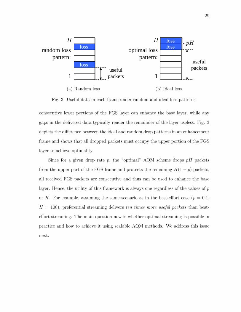
Fig. 3. Useful data in each frame under random and ideal loss patterns.

consecutive lower portions of the FGS layer can enhance the base layer, while any

gaps in the delivered data typically render the remainder of the layer useless. Fig. 3

depicts the difference between the ideal and random drop patterns in an enhancement

frame and shows that all dropped packets must occupy the upper portion of the FGS

layer to achieve optimality.

Since for a given drop rate p, the “optimal” AQM scheme drops pH packets

from the upper part of the FGS frame and protects the remaining H(1− p) packets,

all received FGS packets are consecutive and thus can be used to enhance the base

layer. Hence, the utility of this framework is always one regardless of the values of p

or H. For example, assuming the same scenario as in the best-effort case (p = 0.1,

H = 100), preferential streaming delivers ten times more useful packets than best-

effort streaming. The main question now is whether optimal streaming is possible in

practice and how to achieve it using scalable AQM methods. We address this issue

next.

30

C. Preferential Video Streaming Framework

In this section, we introduce a new video streaming framework called Partitioned

Enhancement Layer Streaming (PELS) that operates in conjunction with priority-

queuing AQM routers in network paths. In the PELS framework, applications parti-

tion the enhancement layer into two layers and voluntarily mark their packets using

different priority classes, allowing the network routers to discriminate between the

packets based on their priority (no per-flow management is required).

Recall that coded video frames carry information that has different importance to

the end user – the lower layers are more sensitive to packet loss than the higher layers.

The base layer (being most sensitive) is required for displaying video appropriately

at the receiver and thus is transmitted using the highest priority class. This ensures

that the base layer is dropped only when the entire FGS layer is discarded by the

routers.

The reason for splitting the FGS layer into two priorities is also simple to un-

derstand. Bytes in the lower part of the FGS layer are more important than those

in the higher part because the former includes the information needed to properly

decode the latter. Due to this nature of FGS streams, dropping packets randomly

(as in the best-effort network) does not properly protect the lower parts of FGS even

under moderate congestion. Hence, to protect the lower portions of FGS frames and

drop the upper parts, preferential treatment of not only the base layer, but also the

enhancement layer is highly desirable.

1. Router Queue Management

We discuss queuing disciplines necessary to support PELS and how applications

should assign priority to their packets. To separate video traffic from the rest of

31

red

yellow

green

PELS queue

linkWRR

1−f

fFIFOInternet queue

Fig. 4. Router queues for PELS framework.

the flows, the proposed PELS architecture must maintain in each network router two

types of queues – the PELS queue and the Internet queue. The PELS queue is further

subdivided into green, yellow, and red priority queues to service marked multimedia

packets, while the Internet queue serves all other (non-multimedia) Internet traffic

in a regular FIFO fashion. To ensure that network bandwidth is shared “fairly” be-

tween PELS applications and other Internet traffic, we employ weighted round-robin

(WRR) scheduling between the PELS and Internet queues. Recall that WRR can

provide a desired level of fairness between several types of traffic by allocating a cer-

tain fraction of the outgoing link to each queue as shown in Fig. 4. This allows

de-centralized administrative flexibility in selecting the weights and assigning proper

“importance” to different classes of traffic.

It is easy to see that the PELS queue must employ a strict priority queuing

discipline to maximize the resulting video quality for a given total throughput budget.

Since the higher parts of the FGS frame cannot be decoded without the presence of

the lower parts, each router has no reason to transmit the higher parts before sending

the lower ones. This implies that network routers must use queuing mechanisms

that do not allow low-priority packets to pass until all high-priority packets are fully

transmitted. Note that, in general, strict priority queueing is frowned upon since

32

it leads to starvation in low-priority queues and denial-of-service effects for certain

flows; however, this situation does not arise in PELS since each flow sends a certain

amount of high-priority (i.e., green) packets and always receives non-negligible service

from the network. In fact, starvation in low-priority (i.e., red) queues is equivalent

to 100% loss in these queues and has very little effect on the resulting quality since

it affects only the upper parts of each enhancement frame (more on this below).

Since PELS application sources can arbitrarily mark their packets, we must next

ensure that no end-user gains anything by marking all of its FGS packets with high

priority (i.e., green). Such “misbehaving” sources will increase congestion in the green

queues, which will result in (uniform) random losses in their base layers and will

quickly degrade the resulting quality of their own video. Similarly, end-flows have

little incentive in sending too many yellow packets or being congestion-indifferent.

Thus, if each application is a selfish, independent entity that attempts to maximize

the utility of its video at the receiver, it will send red packets to probe for congestion

and back-off (i.e., reduce the total sending rate) during the loss of any red packets to

protect the yellow/green queues from upcoming congestion.

We should make several other interesting observations. First, notice that PELS

assumes certain stationarity of the end-to-end path (all packets take the same route)

and the presence of PELS-enabled AQM at the bottleneck router. The former assump-

tion is common to all flows using congestion control (i.e., multi-path routing and/or

route changes make the control loop produce unpredictable results). The latter as-

sumption is very relaxed since it does not require all routers to deploy PELS at the

same time. Our second observation is that priority queuing in PELS is low-overhead,

flexible, does not require support from DiffServ or use of per-flow management, and

can be implemented using priority queues available in many existing router hard-

ware/software solutions. Finally, PELS does not require communication between

33

bi

frame i

transmitted size xi

red: γxi

yellow: (1—γ)xi

discarded

Fig. 5. Partitioning of the FGS layer into two layers and PELS coloring of FGS packets.

routers and leaves the decisions of how to mark packets to the end-user (i.e., pushes

complexity outside the network).

2. FGS Partitioning and Packet Coloring

In a practical network environment (such as the Internet), packet loss and available

bandwidth are not constant and change dynamically depending on cross traffic, link

quality, routing updates, etc. Hence, streaming servers must often probe for newly

available bandwidth as part of congestion control and continuously send low-priority

packets under the assumption that these probes (and only they) will get lost during

congestion.

Fig. 5 illustrates one possible partitioning of FGS bytes into two priority classes

(i.e., yellow and red) that can achieve “optimal” utility discussed in section 2.. The

figure shows that the server sends xi bytes from each enhancement frame i (where xi

is given by congestion control and is derived from Rmax using rate scaling algorithms

[17]). The transmitted section of each FGS frame is divided into two segments – the

lower segment of size (1 − γ)xi is all yellow and the upper segment of size γxi is all

red. The division into red and yellow packets depends on how conservative (many

34

red packets and large γ) or optimistic (few red packets and small γ) the server wants

to be.

In an ideal network with stationary packet loss p in the enhancement layer, the

server can select γ such that γxi is equal to pxi. This will ensure that all red packets

are lost and that exactly (1− p)xi yellow packets are recovered for decoding (this is

the best scenario under any circumstances). In practice, however, keeping red packet

loss pR at 100% is not feasible since any slight increase in p (caused by a new flow

joining the network or change in network conditions) will “spill” the loss into the

yellow queue, effectively creating a best-effort FIFO situation in the yellow queue.

Thus, proper and dynamic selection of γ is important (see the next section).

The other issue to address is congestion control. Even though red queues can be

used to isolate increasing packet loss p without reducing the sending rate of the flow

(i.e., by proportionally increasing γ), the resulting situation will lead to “trashing”

the network with numerous red packets that eventually get dropped at the bottleneck

link. To prevent waste of bandwidth on the path to the bottleneck, the server must

implement elastic congestion control and reduce its rate whenever it loses either yellow

or red packets (the loss of green packets means that there is not enough bandwidth

to support the base layer and no meaningful streaming can continue). Since all flows

in our model use PELS and the same congestion control, they all back-off during the

loss of red packets and keep the amount of “waste” to a minimum.

3. Selection of γ

Recall that partitioning of the FGS layer into yellow/red packets attempts to ensure

that only the upper sections of each frame are dropped during congestion; however,

the performance of PELS depends on the selection of γ and the level of congestion

at the bottleneck link. In order for PELS to be effective, we must ensure that when

35

flows probe for new bandwidth, they do not incur such high levels of congestion as

to force packet loss in the yellow priority queue. Hence, given any control interval k

with packet loss p(k) in the FGS layer, how can the server make sure that there will

be no loss among yellow packets during interval k + 1?

Intuitively, γ should be adjusted according to packet loss measured during in-

terval k to keep the resulting red loss pR = pxi/γxi = p/γ at a certain threshold

pthr. The most optimistic approach suggests pthr ≈ 1 (which leads to the largest

utility U ≈ 1) and the most pessimistic approach keeps pthr ≈ p (which leads to the

best-effort utility in the enhancement layer).

Based upon these observations, we seek a middle ground in which pthr can be

stabilized between 70 and 90% using simple closed-loop control methods that adjust

γ based on the following rules:

• Increase γ when p increases

• Decrease γ when p decreases.

Considering this general intuition, we next investigate a single proportional controller

that adjusts γ based on the measured packet loss p(k) and target red packet loss pthr:

γi(k) = γi(k − 1) + σ(pi(k − 1)/pthr − γi(k − 1)), (14)

where index i represents flow number, pi(k) is the measured average packet loss in

the entire FGS layer for flow i during interval k, and σ is controller’s gain parameter.

Note that (1 − pthr)γxi is the amount of cushion left by the server for the yellow

packets. For example, pthr = 0.75 means that 25% of the red queue works to protect

the yellow queue against sudden (unexpected) increase in packet loss.

Note that, in general, the measurement of pi(k) is coupled with congestion control

and should be provided by its feedback loop (we discuss this in section D.). Next

36

notice that the controller in (14) is stable if the following is satisfied.

Lemma 2. The controller (14) is stable iff 0 < σ < 2.

Proof. Taking the z -transform of (14) we obtain the following:

Γi(z) = z−1Γi(z) + σ(z−1Pi(z)/pthr − z−1Γi(z)

)=

σz−1Pi(z)/pthr

1− (1− σ)z−1. (15)

The poles of system (14) are the roots of its characteristic equation 1−(1−σ)z−1 = 0

(notice that Pi(z) does not depend on Γi(z)). Thus, the system has single pole

z = 1 − σ. For the control system to be stable, the absolute value of z must be less

than 1 (i.e., |z| < 1). This leads to 0 < σ < 2 and concludes the proof.

Note that in a real network environment, feedback delays are often involved.

Assuming arbitrary round-trip delay Di for flow i, (14) becomes:

γi(k) = γi(k −Di) + σ(pi(k −Di)/pthr − γi(k −Di)). (16)

Then we have a stronger version of the previous lemma that shows stability of the

resulting controller under arbitrary delays.

Lemma 3. The controller (16) is stable iff 0 < σ < 2.

Proof. The z -transform of (16) is:

Γi(z) = z−DiΓi(z) + σ(z−DiPi(z)/pthr − z−DiΓi(z)

)=

σz−DiPi(z)/pthr

1− (1− σ)z−Di. (17)

The new pole is given by z = (1− σ)1/Di , which also leads to stability condition

0 < σ < 2.

Next, we derive the effect that (14)-(16) have on the packet loss in the red queues.

Lemma 4. Assuming stationary packet loss p, both controllers (14)-(16) converge

red packet loss pR to pthr.

37

10 20 30 40 50 600.5

0.55

0.6

0.65

0.7

Time (seconds)

g

s = 0.5

10 20 30 40 50 600.5

0.55

0.6

0.65

0.7

0.75

0.8

Time (seconds)

g

s = 2

Fig. 6. Stability of γ with different σ.

Proof. Since γ(k) does not change with time in the steady state, γ(k) = γ(k−1) = γ∗.

From (14), we get:

γ∗ =p∗

pthr

, (18)

where p∗ is the stationary packet loss of the network. Since the red packet-loss can

be expressed as pR(k) = p(k)/γ(k), the stationary red packet-loss is given by:

p∗R =p∗

γ∗. (19)

Substituting γ∗ from (18) into (19), we get p∗R = pthr.

To illustrate that selection of σ is important, but not drastically difficult, Fig. 6

depicts the behavior of γ(k) with different σ (we use a heavy-loss case with p = 0.5

and pthr = 0.75 in this example). As the figure shows, γ(k) is stabilized at the

stationary point γ∗ = p/pthr ≈ 0.67 when σ = 0.5, while it is unstable when σ = 2.

The resulting utility of received video in PELS under dynamically changing γ

is lower-bounded by the following (assuming that only yellow packets are recovered

from the FGS layer):

38

U ≥ H(1− γ)

H(1− p)=

1− p/pthr

1− p. (20)

Thus, the utility of PELS is at least 0.96 for p = 0.1 and pthr = 0.75 and at least 0.996

for p = 0.01 and the same threshold. Although PELS does not achieve “optimality”

for pthr < 1, it comes very close to it and at the same time avoids the pitfalls of the

optimal method.

D. Congestion Control for Video

Congestion control is necessary for streaming applications to provide a high level of

video quality to end users and avoid wasting network resources with packets that are

eventually dropped in congested queues. Many control methods dynamically adjust

the sending rate of end-flows based on network feedback and aim to achieve a stable

tradeoff between under-utilization of resources and network congestion (i.e., packet

loss).

Recent studies have focused on developing smooth congestion control schemes

for multimedia streaming (e.g., TFRC [28] and binomial algorithms [6]) after AIMD

(Additive Increase, Multiplicative Decrease) was unofficially found to be “unaccept-

able” for video streaming due to its large rate fluctuations. Nonetheless, these new

control schemes often do not have stationary points in the operating range of typical

applications and continuously oscillate [107].

Among many recent game-theoretic and optimization methods [46], [51], [53],

[65], [67], [68], [66], [71], we selected Kelly’s congestion control framework (called

proportional fairness [51]), since it is stable, efficient, and fair under various network

conditions. In this section, we study Kelly’s controls, apply them to PELS stream-

ing, and investigate whether their performance provides the necessary foundation for

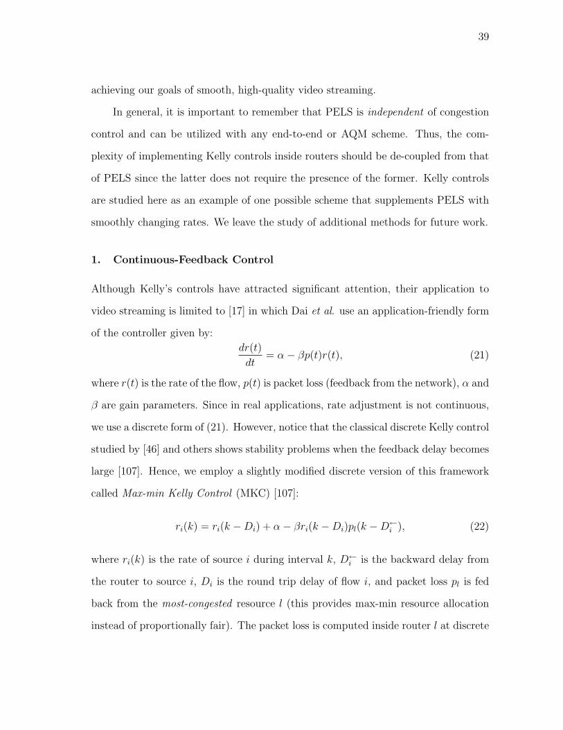
39

achieving our goals of smooth, high-quality video streaming.

In general, it is important to remember that PELS is independent of congestion

control and can be utilized with any end-to-end or AQM scheme. Thus, the com-

plexity of implementing Kelly controls inside routers should be de-coupled from that

of PELS since the latter does not require the presence of the former. Kelly controls

are studied here as an example of one possible scheme that supplements PELS with

smoothly changing rates. We leave the study of additional methods for future work.

1. Continuous-Feedback Control

Although Kelly’s controls have attracted significant attention, their application to

video streaming is limited to [17] in which Dai et al. use an application-friendly form

of the controller given by:

dr(t)

dt= α− βp(t)r(t), (21)

where r(t) is the rate of the flow, p(t) is packet loss (feedback from the network), α and

β are gain parameters. Since in real applications, rate adjustment is not continuous,

we use a discrete form of (21). However, notice that the classical discrete Kelly control

studied by [46] and others shows stability problems when the feedback delay becomes

large [107]. Hence, we employ a slightly modified discrete version of this framework

called Max-min Kelly Control (MKC) [107]:

ri(k) = ri(k −Di) + α− βri(k −Di)pl(k −D←i ), (22)

where ri(k) is the rate of source i during interval k, D←i is the backward delay from

the router to source i, Di is the round trip delay of flow i, and packet loss pl is fed

back from the most-congested resource l (this provides max-min resource allocation

instead of proportionally fair). The packet loss is computed inside router l at discrete

40

intervals and inserted into all passing packets:

pl(k) =

∑j∈Sl

rj(k −D→j )− Cl∑

j∈Slrj(k −D→

j ), (23)

where Sl is the set of sources sending packets through router l, D→j is the forward

delay from source j to the router, and Cl is link capacity of router l. The stability of

system (22)-(23) is formalized as follows.

Lemma 5. System (22)-(23) is stable under heterogeneous delays iff 0 < β < 2.

Proof. See [107].

We apply (22) for rate control in PELS streaming and investigate its control

characteristics including:

• Convergence to a single stationary point

• Fairness between flows.

From (22) and (23), we next derive stationary rates r∗i of end flows in the equilibrium

point and show that (22) has no oscillations in the steady state.

Lemma 6. Regardless of the feedback delay, the stationary rate r∗i of each flow is:

r∗i =Cl

N+

α

β. (24)

Proof. Since the rate of each flow does not change with time in the steady state,

ri(k) = ri(k −Di) = r∗i . Using this observation in (22) we get

r∗i =α

βp∗, (25)

where p∗ is the stationary packet loss. Since in the steady state, all flows share the

bandwidth equally (i.e., r∗i = r∗j = r∗), we have p∗ =Nr∗ − C

Nr∗from (23). Substituting

p∗ =Nr∗i − C

Nr∗iin (25) and rearranging it we get (24).

41

Thus, unlike AIMD or TCP, MKC does not penalize flows with higher RTT and

further converges to a single stationary point with no oscillation.

Next notice that priority queueing in PELS imposes increased delays on red

packets and that the utilization of each priority class directly affects delay charac-

teristics of all queues with lower priority. Since green packets have much smaller

queuing delays than yellow or red packets, it is tempting to provide feedback only in

green packets. However, since the base layer is sent at significantly lower rates than

the enhancement layer, this method introduces unnecessary feedback delays due to

large inter-packet spacing of the base layer. Thus, it is easy to conclude that network

feedback must be inserted by the router into all passing packets (regardless of their

color) for timely delivery to the end flows. Below, we discuss methods to discard

out-of-sequence (i.e., outdated) feedback that may arrive in red/yellow packets.

2. PELS Implementation

We implemented new agents and a priority-based AQM mechanism for PELS stream-

ing in the ns2 network simulator [73]. PELS application sources mark their packets

with three priority levels (i.e., green, yellow, and red) and employ MKC for rate

control. Computation of packet loss p(k) is performed by the router on a discrete

time scale of T time units and then injected into the header of each packet passing

through the router (note that feedback information is a queue-specific metric). Each

new computation of p(k) increases router’s local epoch number z to prevent sources

from reacting to the same feedback more than once as well as to suppress outdated

values of p(k) created by re-ordering inside PELS queues. Label (router ID, z, p(k))

is provided to end flows through the header of the packets queued at the bottleneck

link.

Once received by the end-user, feedback p(k) is sent in ACKs to the source, which

42

applies rate adjustments according to (22) as long as it has not seen this feedback

before. The use of epoch numbers allows the source to keep the frequency of its

control loop in sync with that of the router and ensures stability of the resulting

system.

We next describe the above two algorithms in more detail. Upon arrival and

queuing of a packet j, the router increments its local counter S by the size sj of the

packet: S = S + sj. Then once every T time units, the router computes new total

rate R, new packet loss p, increments its epoch number z, and resets the byte counter:

R =S

T, p =

R− C

R, z = z + 1, S = 0. (26)

To verify the “freshness” of feedback, each PELS source i checks feedback se-

quence number z in the acknowledgment and ignores feedback with z less than or

equal to its current epoch number zi; otherwise, zi is set to z and a new sending

rate is computed using (22). When there are multiple routers along an end-to-end

path, each router compares its pl with that inside arriving packets and overrides the

existing value only if its packet loss is larger than the current loss recorded in the

header. End flows use the router ID field to keep track of feedback freshness and

react to possible shifts of the bottlenecks.

Selection of interval T depends on the desired responsiveness of the PELS frame-

work to network conditions, but does not affect stability of the system as a whole.

To analytically reflect the implementation of the PELS framework where the router

purposely delays its feedback by T units, we need to modify the model of packet loss

in (23) to become:

pl(k) =

∑j∈Sj

rj(k − T −D→j )− Cl∑

j∈Sjrj(k − T −D→

j ). (27)

Stability of system (22)-(27) is proved using the same arguments as in Lemma 5 [107]

43

R1

R2

4 mb/s

10 mb/s

10 mb/s

10 mb/s

10 mb/s

.

.

.

PELS

NS

PELSS

1

TCP

MS

TCPS

1

.

.

.

.

.

.

PELS

NR

PELSR

1

TCP

MR

TCPR

1

.

.

.

Fig. 7. Simulation topology.

and is omitted from this work.

E. Simulation Results

In this section, we present simulation results of PELS including the properties of γ(k),

MKC congestion control, PELS queuing delay, and PELS video quality. We start by

describing the simulation setup.

1. Simulation Setup

For ns2 simulations, we use a simple bar-bell topology with multiple PELS and TCP

sources connecting to a single bottleneck link. As shown in Fig. 7, the capacity of

the bottleneck is 4 mb/s, while the rest of the links are 10 mb/s. In all simulations,

one video frame (63, 000 bytes including the base layer) consists of 126 packets, 500

bytes each (these numbers are derived from MPEG-4 coded CIF Foreman). We mark

21 packets in each frame as green to protect the base layer of the sequence.

Recall that router queues in our framework completely separate the PELS flows

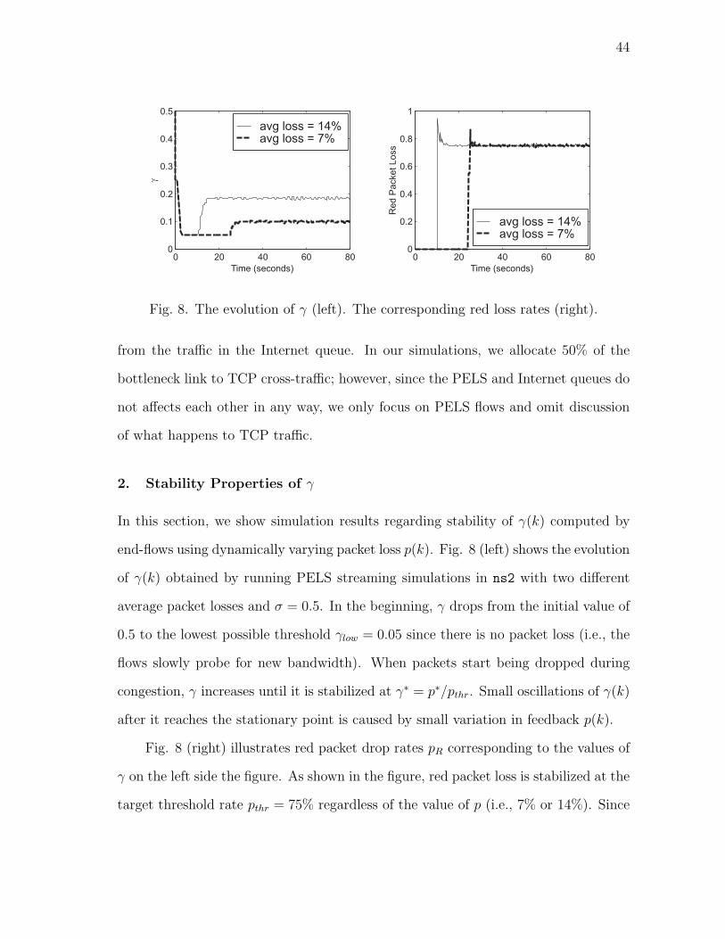
44

0 20 40 60 800

0.1

0.2

0.3

0.4

0.5

Time (seconds)

g

avg loss = 14%avg loss = 7%

0 20 40 60 800

0.2

0.4

0.6

0.8

1

Time (seconds)

Re

d P

acke

t L

oss

avg loss = 14%avg loss = 7%

Fig. 8. The evolution of γ (left). The corresponding red loss rates (right).

from the traffic in the Internet queue. In our simulations, we allocate 50% of the

bottleneck link to TCP cross-traffic; however, since the PELS and Internet queues do

not affects each other in any way, we only focus on PELS flows and omit discussion

of what happens to TCP traffic.

2. Stability Properties of γ

In this section, we show simulation results regarding stability of γ(k) computed by

end-flows using dynamically varying packet loss p(k). Fig. 8 (left) shows the evolution

of γ(k) obtained by running PELS streaming simulations in ns2 with two different

average packet losses and σ = 0.5. In the beginning, γ drops from the initial value of

0.5 to the lowest possible threshold γlow = 0.05 since there is no packet loss (i.e., the

flows slowly probe for new bandwidth). When packets start being dropped during

congestion, γ increases until it is stabilized at γ∗ = p∗/pthr. Small oscillations of γ(k)

after it reaches the stationary point is caused by small variation in feedback p(k).

Fig. 8 (right) illustrates red packet drop rates pR corresponding to the values of

γ on the left side the figure. As shown in the figure, red packet loss is stabilized at the

target threshold rate pthr = 75% regardless of the value of p (i.e., 7% or 14%). Since

45

0 100 200 3000.012

0.014

0.016

0.018

0.02

0.022

Time (seconds)

Dela

y (

seconds)

0 100 200 3000.01

0.015

0.02

0.025

0.03

0.035

Time (seconds)

Dela

y (

seconds)

Fig. 9. Green (left) and yellow (right) delays.

the red loss never reaches 100%, all of yellow packets are protected and experience

(ideal) zero-loss conditions.

Recall that AQM routers in the PELS framework employ three priority queues

for preferential treatment of green, yellow, and red packets. Fig. 9 illustrates delays

of green (left) and yellow (right) packets and Fig. 10 (left) depicts delays of red

packets. Theses delays are obtained by running ns2 simulations in which at every 50

seconds, two new flows entered the system with the initial rate of 128 kb/s (i.e., the

rate of the base layer).

3. Delay Characteristics of PELS

First notice that green and yellow packets have very small delays compared to those

of red packets. The average delays of green and yellow packets are only 16 and 25 ms,

respectively, while the average delays of red packets reach as high as 400 ms. Further

notice that after 100 seconds, red packet delays increase every 50 seconds since each

new flow further reduces the available bandwidth and increases congestion in the red

queue. These results are expected from the use of priority queuing in the routers

and have no harmful effect on PELS flows as loss or delays in the red queue have

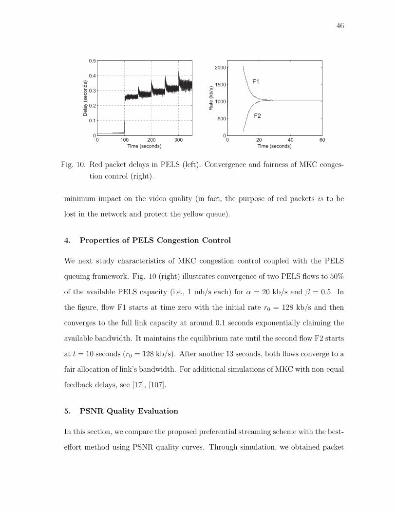
46

0 20 40 600

500

1000

1500

2000

F1

F2

Time (seconds)

Ra

te (

kb

/s)

0 100 200 3000

0.1

0.2

0.3

0.4

0.5

Time (seconds)

De

lay (

se

co

nd

s)

Fig. 10. Red packet delays in PELS (left). Convergence and fairness of MKC conges-

tion control (right).

minimum impact on the video quality (in fact, the purpose of red packets is to be

lost in the network and protect the yellow queue).

4. Properties of PELS Congestion Control

We next study characteristics of MKC congestion control coupled with the PELS

queuing framework. Fig. 10 (right) illustrates convergence of two PELS flows to 50%

of the available PELS capacity (i.e., 1 mb/s each) for α = 20 kb/s and β = 0.5. In

the figure, flow F1 starts at time zero with the initial rate r0 = 128 kb/s and then

converges to the full link capacity at around 0.1 seconds exponentially claiming the

available bandwidth. It maintains the equilibrium rate until the second flow F2 starts

at t = 10 seconds (r0 = 128 kb/s). After another 13 seconds, both flows converge to a

fair allocation of link’s bandwidth. For additional simulations of MKC with non-equal

feedback delays, see [17], [107].

5. PSNR Quality Evaluation

In this section, we compare the proposed preferential streaming scheme with the best-

effort method using PSNR quality curves. Through simulation, we obtained packet

47

loss statistics of each FGS frame and then applied them to the video sequence offline.

We enhanced each base-layer frame using consecutively received FGS packets and

plotted PSNR quality curves accordingly. Aggregate packet loss was calculated in

the routers at T = 30 ms time intervals.

Our main puzzle in this section was to properly select a “generic” brand of best-

effort streaming that adequately represents existing (non-QoS) approaches. Although

there are numerous methods of streaming video over the Internet (including TCP,

FEC-protected transmission, and various non-AIMD methods), we aim to compare

PELS with an alternative framework that: 1) does not retransmit any lost packets;

and 2) does not send any error-correcting codes. Since no such framework exists to

our knowledge, we use AQM-enabled MKC under the assumption that the base layer

is “magically” protected at all times. If packet loss is allowed in the base layer and

retransmission is suppressed, best-effort streaming simply becomes impossible due to

propagation of losses throughout each GOP (Group of Pictures). Thus, we protected

the entire base layer in the best-effort case and allowed random loss only in the FGS

layer to keep this approach even remotely competitive with PELS.

We first examine PSNR of the Foreman sequence reconstructed with 10% network

packet loss (Fig. 11(a)). As shown in the figure, best-effort streaming improves the

base-layer PSNR by approximately 24% on average, while PELS enhances it by 60%.

Next, we examine the case with higher packet loss. Fig. 11(b) illustrates the

PSNR curve of the same Foreman sequence reconstructed with 19% packet loss. In

this case, while the best-effort method improves the base-layer PSNR only by 16%,

PELS improves it by 55%.

From the curves in Fig. 11, we also observe that the PSNR of best-effort stream-

ing varies by as much as 15 dB (even though the sending rates of MKC are perfectly

smooth) and provides a highly-fluctuating quality that is similar to that achievable

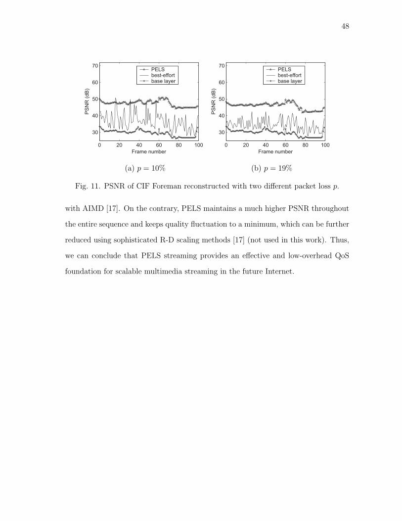
48

0 20 40 60 80 100

30

40

50

60

70

Frame number

PS

NR

(d

B)

PELSbest-effortbase layer

(a) p = 10%

0 20 40 60 80 100

30

40

50

60

70

Frame number

PS

NR

(d

B)

PELSbest-effortbase layer

(b) p = 19%

Fig. 11. PSNR of CIF Foreman reconstructed with two different packet loss p.

with AIMD [17]. On the contrary, PELS maintains a much higher PSNR throughout

the entire sequence and keeps quality fluctuation to a minimum, which can be further

reduced using sophisticated R-D scaling methods [17] (not used in this work). Thus,

we can conclude that PELS streaming provides an effective and low-overhead QoS

foundation for scalable multimedia streaming in the future Internet.

49

CHAPTER IV

MODELING BEST-EFFORT AND FEC STREAMING

We study Forward-Error Correction (FEC) for video streaming over best-effort net-

works. FEC is often used in streaming applications to protect video and audio data in

lossy network paths; however, studies (such as [3], [7], [11], [31]) in the literature re-

port conflicting results on the benefits of FEC over best-effort streaming. To address

this uncertainty, we start with a baseline case that examines the impact of packet

loss on scalable (FGS-like) video in best-effort networks and derive a closed-form ex-

pression for the loss penalty imposed on embedded coding schemes under several loss

models. Through this analysis, we find that the utility (i.e., usefulness to the user) of

unprotected video converges to zero as streaming rates become high. We then study

FEC-protected video streaming, re-derive the same utility metric, and show that for

all values of loss rate inclusion of FEC overhead substantially improves the utility

of video compared to the best-effort case. We finish this chapter by constructing a

dynamic controller on the amount of FEC that maximizes the utility of scalable video

and show that the resulting system achieves a significantly better PSNR quality than

alternative fixed-overhead methods.

A. Introduction

Forward-error correction (FEC) is widely used in the Internet for its ability to recover

data segments lost in the network [7], [79], [103]. With a proper amount of redun-

dancy included in transmitted packets, FEC can reduce the impact of packet loss on

the quality of video, thus improving the performance of streaming over best-effort

50

networks. However, selection of FEC overhead becomes a fairly complicated task

when network path dynamics change over time, which in certain cases may lead to

reduced or negligible performance gain compared to similar best-effort scenarios [3],

[7], [58].

Although FEC appears intuitively beneficial, studies in the literature report con-

flicting results on its performance in practice. Some of them (e.g., [3], [58]) show that

FEC provides little benefit to applications due to the extra overhead, while others

(e.g., [11], [31]) find FEC to be promising in the context of particular multimedia ap-

plications. To understand the benefits of FEC in Internet streaming, we first analyze

the performance of video streaming in best-effort networks and derive a closed-form

model for the penalty inflicted on scalable1 video coding under Markov and renewal

patterns of packet loss. For this analysis, we consider end-user utility U as the main

metric, which we define as the percentage of received data in each frame that can be

used for decoding the frame, i.e.,

U =M

T, (28)

where M is the average number of bytes/packets used in decoding a frame and T

is the average amount of data per frame successfully delivered to the receiver. De-

riving (28) in closed-form, we show that best-effort streaming imposes a significant

penalty on video applications when packet loss randomly corrupts the video stream

and demonstrate that for any fixed packet loss p > 0, the utility U → 0 as the

streaming rate goes to infinity.

Given poor performance of best-effort streaming, we next examine FEC-protected

1In scalable video (e.g., MPEG-4 FGS [83]), the enhancement layer is compressedusing embedded coding and can be easily re-scaled to match variable network band-width during streaming. In such methods, the lower sections of the enhancement layerare more important than the higher sections because their loss renders all dependentdata in the source frame virtually useless.

51

transmission of video data. Previous studies in the literature (e.g., [31], [32], [105])

have examined the dynamics of the loss process under a two-state Markov chain

and provided numerical models for obtaining the distribution of the number of loss

events in a block of fixed size n; however, these models usually rely on complex re-

cursive expressions or tedious summations, neither of which sheds light in qualitative

or closed-form terms on the behavior of FEC in practice. To overcome this limitation

and ultimately compute (28), we study the effect of Markov-based packet loss within

an FEC block and derive the asymptotic (i.e., assuming large sending rates) distribu-

tion of the number of lost packets per FEC block. This model offers a low-complexity

version of the same result obtained by the earlier methods and allows computation

of other metrics of interest related to FEC streaming.

Armed with this result, we next focus on investigating the performance of video

streaming with FEC protection under two-state Markov-chain loss. Assuming that

R is the streaming rate of the application and F is the rate of FEC packets, we

employ (28) to understand how the FEC overhead rate ψ = F/(R + F ), (0 < ψ < 1),

affects the utility of received video. Using the models derived in the second part of the

chapter, we show that U exhibits percolation and converges to 0, 0.5, or (1−ψ)/(1−p)

depending on the value of ψ as the streaming rate R approaches infinity. However,

for finite R, we find that U achieves a unique global maximum in some point ψ∗ that

depends on network packet loss and FEC block size, which indicates that sending

more or less FEC than the optimal amount results in a reduction in U .

Driven by the goal of maximizing the usefulness of network bandwidth and

achieving the highest visual quality under given network conditions, we subsequently

explore a simple control mechanism that dynamically adjusts the amount of overhead

ψ(t) based on the packet-loss information fed back to application servers by their

receivers. We find that such adaptive control allows the application to maintain op-

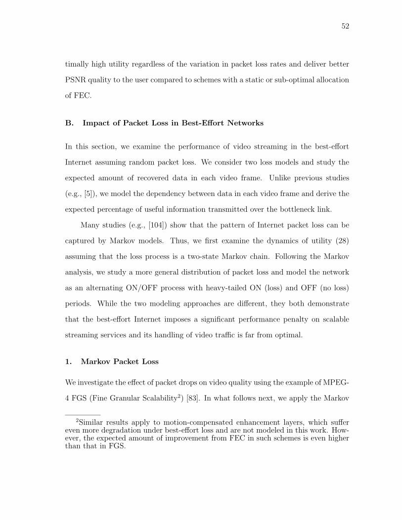
52

timally high utility regardless of the variation in packet loss rates and deliver better

PSNR quality to the user compared to schemes with a static or sub-optimal allocation

of FEC.

B. Impact of Packet Loss in Best-Effort Networks

In this section, we examine the performance of video streaming in the best-effort

Internet assuming random packet loss. We consider two loss models and study the

expected amount of recovered data in each video frame. Unlike previous studies

(e.g., [5]), we model the dependency between data in each video frame and derive the

expected percentage of useful information transmitted over the bottleneck link.

Many studies (e.g., [104]) show that the pattern of Internet packet loss can be

captured by Markov models. Thus, we first examine the dynamics of utility (28)

assuming that the loss process is a two-state Markov chain. Following the Markov

analysis, we study a more general distribution of packet loss and model the network

as an alternating ON/OFF process with heavy-tailed ON (loss) and OFF (no loss)

periods. While the two modeling approaches are different, they both demonstrate

that the best-effort Internet imposes a significant performance penalty on scalable

streaming services and its handling of video traffic is far from optimal.

1. Markov Packet Loss

We investigate the effect of packet drops on video quality using the example of MPEG-

4 FGS (Fine Granular Scalability2) [83]. In what follows next, we apply the Markov

2Similar results apply to motion-compensated enhancement layers, which suffereven more degradation under best-effort loss and are not modeled in this work. How-ever, the expected amount of improvement from FEC in such schemes is even higherthan that in FGS.

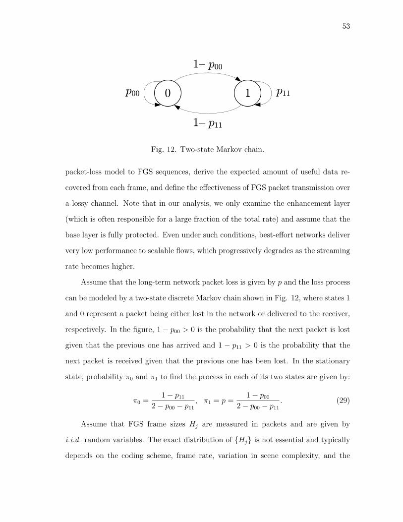
53

0 1

1 p00

p00 p11

1 p11

Fig. 12. Two-state Markov chain.

packet-loss model to FGS sequences, derive the expected amount of useful data re-

covered from each frame, and define the effectiveness of FGS packet transmission over

a lossy channel. Note that in our analysis, we only examine the enhancement layer

(which is often responsible for a large fraction of the total rate) and assume that the

base layer is fully protected. Even under such conditions, best-effort networks deliver

very low performance to scalable flows, which progressively degrades as the streaming

rate becomes higher.

Assume that the long-term network packet loss is given by p and the loss process

can be modeled by a two-state discrete Markov chain shown in Fig. 12, where states 1

and 0 represent a packet being either lost in the network or delivered to the receiver,

respectively. In the figure, 1− p00 > 0 is the probability that the next packet is lost

given that the previous one has arrived and 1 − p11 > 0 is the probability that the

next packet is received given that the previous one has been lost. In the stationary

state, probability π0 and π1 to find the process in each of its two states are given by:

π0 =1− p11

2− p00 − p11

, π1 = p =1− p00

2− p00 − p11

. (29)

Assume that FGS frame sizes Hj are measured in packets and are given by

i.i.d. random variables. The exact distribution of {Hj} is not essential and typically

depends on the coding scheme, frame rate, variation in scene complexity, and the

54

bitrate of the sequence. The question we address next is what is the expected amount

of useful packets that the receiver can decode from each frame under p-percent random

loss? To answer this question, we denote by Zj the number of consecutively received

packets in a frame j and next compute its expectation E[Zj], which plays an important

role in determining the utility of received video.

Assume that the chain is stationary at the beginning of a frame and let E[ZHj ]

be the expected number of useful packets per frame if all frames are of size H. Then,

we have the following result.

Theorem 1. Assuming a two-state Markov packet loss in (29) and fixed-size frames

with Hj = H, the expected number of useful packets in each frame is:

E[ZHj ] =

1− p

1− p00

(1− pH00). (30)

Proof. Assume that Dj is the random distance in packets from the beginning of frame

j before the first packet-loss event. Let X1 be the state of the Markov chain when

the first packet in frame j passes through the network. Note that if X1 = 1, then the

amount of recovered data in the frame is Zj = 0; however, if the loss process is in

state X1 = 0, then the recovered amount depends on the value of Dj, i.e., the decoder

recovers Zj = Dj packets when Dj ≤ H and all Zj = H packets otherwise. Then, we

can write:

E[ZHj ] = π0E[ZH

j |X1 = 0] + π1E[ZHj |X1 = 1]

= π0

( H∑i=1

iP (Dj = i|X1 = 0) + H

∞∑i=H+1

P (Dj = i|X1 = 0))

(31)

Conditioning on X1 = 0, it immediately follows that Dj are geometric random

variables with a conditional PMF P (Dj = i|X1 = 0) = pi−100 (1 − p00), i ≥ 1. Substi-

tuting π0 = 1− π1 = 1− p in (31) and expanding the PMF of Dj, we get (30).

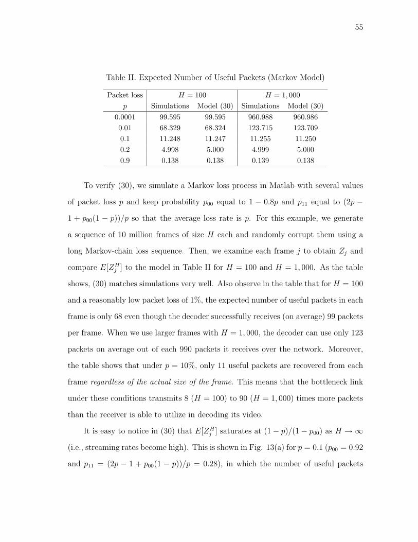
55

Table II. Expected Number of Useful Packets (Markov Model)

Packet loss H = 100 H = 1, 000p Simulations Model (30) Simulations Model (30)

0.0001 99.595 99.595 960.988 960.9860.01 68.329 68.324 123.715 123.7090.1 11.248 11.247 11.255 11.2500.2 4.998 5.000 4.999 5.0000.9 0.138 0.138 0.139 0.138

To verify (30), we simulate a Markov loss process in Matlab with several values

of packet loss p and keep probability p00 equal to 1 − 0.8p and p11 equal to (2p −1 + p00(1 − p))/p so that the average loss rate is p. For this example, we generate

a sequence of 10 million frames of size H each and randomly corrupt them using a

long Markov-chain loss sequence. Then, we examine each frame j to obtain Zj and

compare E[ZHj ] to the model in Table II for H = 100 and H = 1, 000. As the table

shows, (30) matches simulations very well. Also observe in the table that for H = 100

and a reasonably low packet loss of 1%, the expected number of useful packets in each

frame is only 68 even though the decoder successfully receives (on average) 99 packets

per frame. When we use larger frames with H = 1, 000, the decoder can use only 123

packets on average out of each 990 packets it receives over the network. Moreover,

the table shows that under p = 10%, only 11 useful packets are recovered from each

frame regardless of the actual size of the frame. This means that the bottleneck link

under these conditions transmits 8 (H = 100) to 90 (H = 1, 000) times more packets

than the receiver is able to utilize in decoding its video.

It is easy to notice in (30) that E[ZHj ] saturates at (1− p)/(1− p00) as H →∞

(i.e., streaming rates become high). This is shown in Fig. 13(a) for p = 0.1 (p00 = 0.92

and p11 = (2p − 1 + p00(1 − p))/p = 0.28), in which the number of useful packets

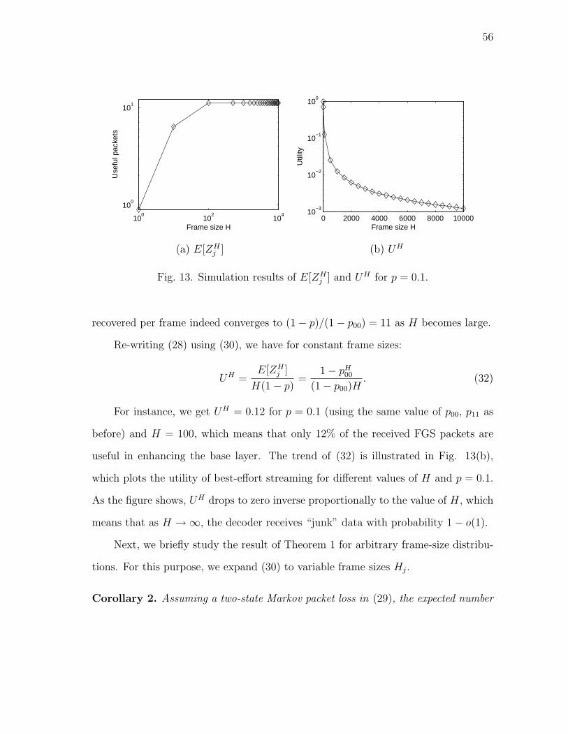
56

100

102

104

100

101

Use

ful p

acke

ts

Frame size H

(a) E[ZHj ]

0 2000 4000 6000 8000 1000010

−3

10−2

10−1

100

Util

ity

Frame size H

(b) UH

Fig. 13. Simulation results of E[ZHj ] and UH for p = 0.1.

recovered per frame indeed converges to (1− p)/(1− p00) = 11 as H becomes large.

Re-writing (28) using (30), we have for constant frame sizes:

UH =E[ZH

j ]

H(1− p)=

1− pH00

(1− p00)H. (32)

For instance, we get UH = 0.12 for p = 0.1 (using the same value of p00, p11 as

before) and H = 100, which means that only 12% of the received FGS packets are

useful in enhancing the base layer. The trend of (32) is illustrated in Fig. 13(b),

which plots the utility of best-effort streaming for different values of H and p = 0.1.

As the figure shows, UH drops to zero inverse proportionally to the value of H, which

means that as H →∞, the decoder receives “junk” data with probability 1− o(1).

Next, we briefly study the result of Theorem 1 for arbitrary frame-size distribu-

tions. For this purpose, we expand (30) to variable frame sizes Hj.

Corollary 2. Assuming a two-state Markov packet loss in (29), the expected number

57

of useful packets in each frame is:

E[Zj] =1− p

1− p00

(1− E[p

Hj

00 ]). (33)

In the next theorem, we show that E[Zj] in any video sequence with the average

frame size H is upper-bounded by (30).

Theorem 3. For a given average frame size E[Hj] = H and Markov-chain loss,

the expected number of useful packets per frame is always upper-bounded by that in

sequences with Hj = H:

E[Zj] ≤ E[ZHj ]. (34)

Proof. Set u(x) = px00 and notice that u(x) is a strictly convex function of x. Then,

using Jensen’s inequality, it follows that E[u(Hj)] is no less than u(E[Hj]) and there-

fore 1−E[pHj

00 ] ≤ 1−pH00. Applying this observation to (30) and (33), we immediately

obtain (34).

We illustrate the result of Theorem 3 assuming a lognormal3 frame-size distribu-

tion, whose PDF is given by:

f(x) =1√

2πσxe−(log x−µ)2/2σ2

, (35)

where µ and σ2 are respectively the mean and variance of log(Hj). For the sake of

this example, we use p = 0.1, p00 = 1−p, σ = 1.5 and compute µ such that the mean

of the lognormal distribution E[Hj] = eµ+σ2/2 matches the desired values. Table III

shows the expected number of useful packets in each frame of this sequence and the

same metric in the case of constant frame sizes Hj = H. As the table shows, E[Zj]

matches simulations well and is in fact upper-bounded by E[ZHj ].

3Several studies have shown that MPEG frame sizes can be modeled by a lognormaldistribution [87], which explains our interest in it.

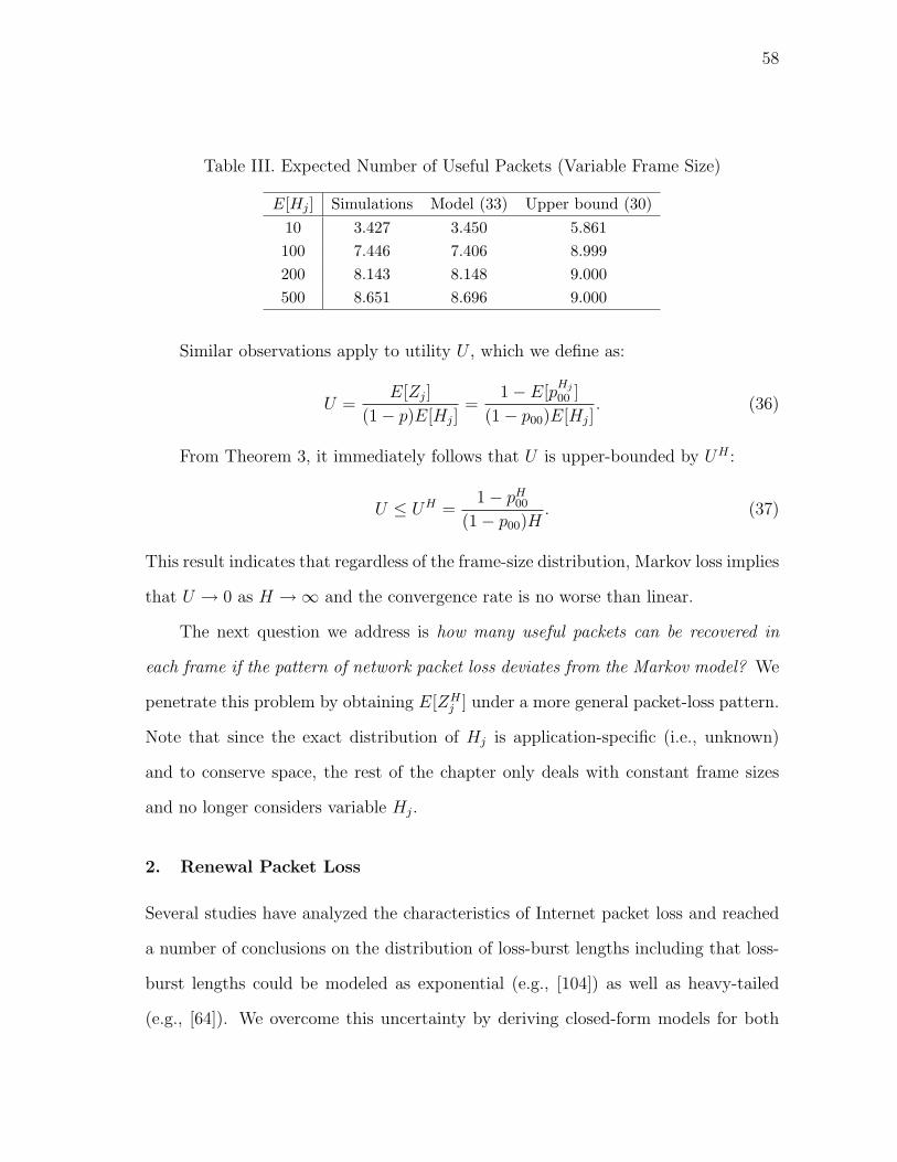
58

Table III. Expected Number of Useful Packets (Variable Frame Size)

E[Hj ] Simulations Model (33) Upper bound (30)10 3.427 3.450 5.861100 7.446 7.406 8.999200 8.143 8.148 9.000500 8.651 8.696 9.000

Similar observations apply to utility U , which we define as:

U =E[Zj]

(1− p)E[Hj]=

1− E[pHj

00 ]

(1− p00)E[Hj]. (36)

From Theorem 3, it immediately follows that U is upper-bounded by UH :

U ≤ UH =1− pH

00

(1− p00)H. (37)

This result indicates that regardless of the frame-size distribution, Markov loss implies

that U → 0 as H →∞ and the convergence rate is no worse than linear.

The next question we address is how many useful packets can be recovered in

each frame if the pattern of network packet loss deviates from the Markov model? We

penetrate this problem by obtaining E[ZHj ] under a more general packet-loss pattern.

Note that since the exact distribution of Hj is application-specific (i.e., unknown)

and to conserve space, the rest of the chapter only deals with constant frame sizes

and no longer considers variable Hj.

2. Renewal Packet Loss

Several studies have analyzed the characteristics of Internet packet loss and reached

a number of conclusions on the distribution of loss-burst lengths including that loss-

burst lengths could be modeled as exponential (e.g., [104]) as well as heavy-tailed

(e.g., [64]). We overcome this uncertainty by deriving closed-form models for both

59

Y1

X1

R(τj)

WiW1

Hτ1 τ2 τj τj + 1

...

loss

process

frames

Fig. 14. ON/OFF process V (t) (top) and the transmission pattern of video frames

(bottom).

cases, as well as the more generic case when loss-burst lengths have an arbitrary

distribution.

We explore the recurrent behavior of packet loss using a simple stochastic model

from renewal theory. Assume that the packet loss process V (t) goes through ON/OFF

periods, where all packets are lost during each ON period and all packets are delivered

during each OFF period. Then, we can write:

V (t) =

1 loss at time t

0 no loss at time t

. (38)

Suppose that the duration of the i-th ON period is given by a random variable Xi

and the duration of the i-th OFF period is given by Yi (Xi and Yi may be drawn from

different distributions). Fig. 14 illustrates the evolution of alternating process V (t).

The figure also shows that if V (t) is sampled at a random instant τj where frame

j starts and the process happens to be in the OFF state, the distance to the next

packet loss is given by some residual process R(τj), whose distribution determines Zj.

We elaborate on this observation next.

60

Assume that Xi and Yi are independent of each other and sets {Xi} and {Yi}consist of i.i.d. random variables. Then, V (t) is an alternating renewal process, whose

j-th renewal cycle has duration Wj = Xj +Yj and whose n-th renewal occurs at time

epoch Tn =∑n

j=1 Wj. Next, we derive long-term network packet loss p, which is the

fraction of time that the process is in the ON state.

Lemma 7. Under the ON/OFF process model, the long-term network packet loss p

is:

p = limt→∞

P (V (t) = 1) =E[Xi]

E[Xi] + E[Yi]. (39)

Proof. Notice that network packet loss is the ratio of the total number of lost packets

to the total number of transmitted packets, averaged over a sufficiently long period

of time. This can be written as:

p = limt→∞

1

t

t∫

0

V (u)du. (40)

We can view each ON duration of V (t) as the amount of reward Pj = Xj for

each renewal cycle Wj. Then, the cumulative reward C(t) of this process over each

interval [0, t) is C(t) =∫ t

0V (u)du. Applying the renewal-reward theorem to C(t), we

have [102]:

p = limt→∞

C(t)

t=

E[Pj]

E[Wj]. (41)

Substituting E[Pj] and E[Wj] in (41), we get (39).

Given network packet loss p, we are primarily interested in the location of the

first ON event after each frame starts, which determines the number of consecutively

received packets in that frame. Suppose that τj represents the time instants when

the j-th frame starts its transmission over the network. Then, we can safely assume

that points τj are uncorrelated with the cycles of packet loss V (t) since the former

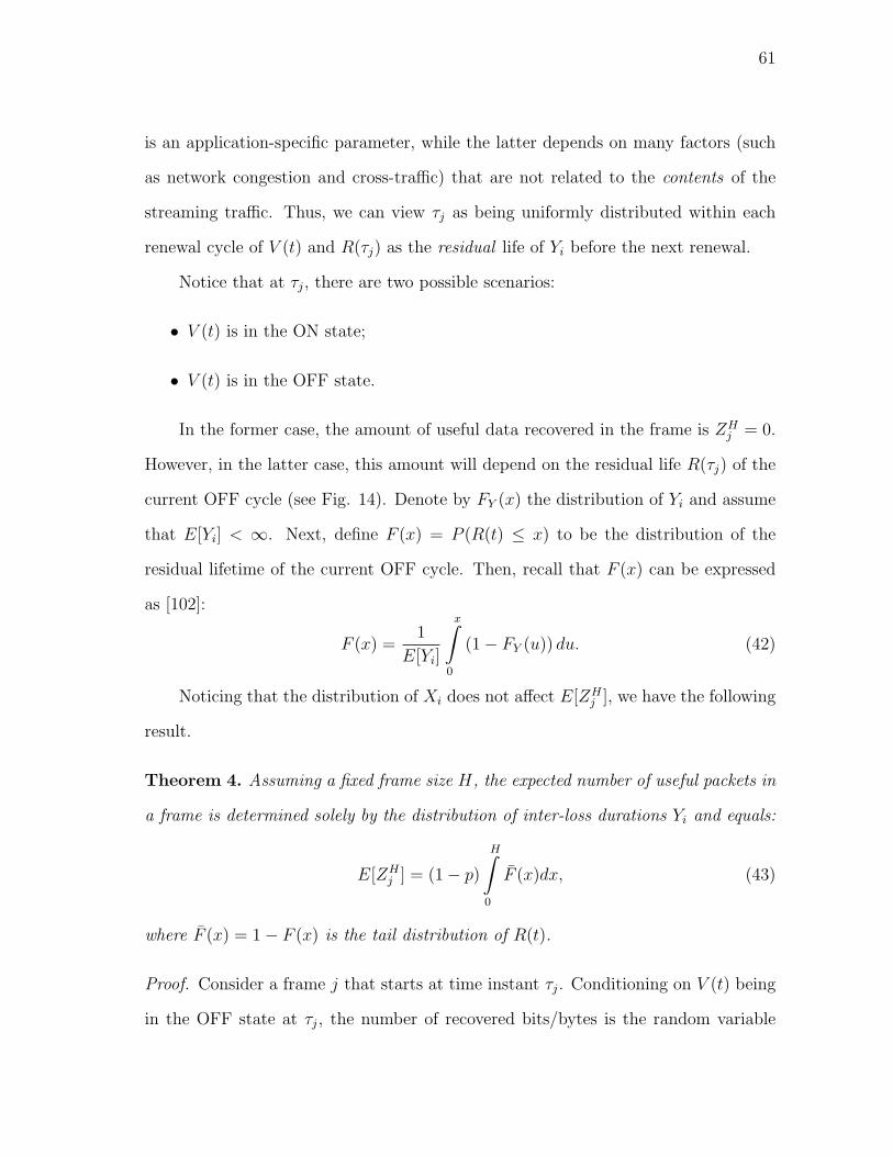
61

is an application-specific parameter, while the latter depends on many factors (such

as network congestion and cross-traffic) that are not related to the contents of the

streaming traffic. Thus, we can view τj as being uniformly distributed within each

renewal cycle of V (t) and R(τj) as the residual life of Yi before the next renewal.

Notice that at τj, there are two possible scenarios:

• V (t) is in the ON state;

• V (t) is in the OFF state.

In the former case, the amount of useful data recovered in the frame is ZHj = 0.

However, in the latter case, this amount will depend on the residual life R(τj) of the

current OFF cycle (see Fig. 14). Denote by FY (x) the distribution of Yi and assume

that E[Yi] < ∞. Next, define F (x) = P (R(t) ≤ x) to be the distribution of the

residual lifetime of the current OFF cycle. Then, recall that F (x) can be expressed

as [102]:

F (x) =1

E[Yi]

x∫

0

(1− FY (u)) du. (42)

Noticing that the distribution of Xi does not affect E[ZHj ], we have the following

result.

Theorem 4. Assuming a fixed frame size H, the expected number of useful packets in

a frame is determined solely by the distribution of inter-loss durations Yi and equals:

E[ZHj ] = (1− p)

H∫

0

F (x)dx, (43)

where F (x) = 1− F (x) is the tail distribution of R(t).

Proof. Consider a frame j that starts at time instant τj. Conditioning on V (t) being

in the OFF state at τj, the number of recovered bits/bytes is the random variable

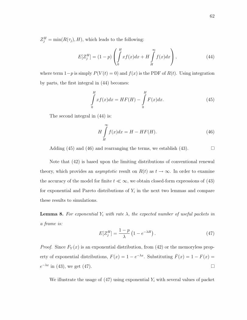
62

ZHj = min(R(τj), H), which leads to the following:

E[ZHj ] = (1− p)

H∫

0

xf(x)dx + H

∞∫

H

f(x)dx

, (44)

where term 1−p is simply P (V (t) = 0) and f(x) is the PDF of R(t). Using integration

by parts, the first integral in (44) becomes:

H∫

0

xf(x)dx = HF (H)−H∫

0

F (x)dx. (45)

The second integral in (44) is:

H

∞∫

H

f(x)dx = H −HF (H). (46)

Adding (45) and (46) and rearranging the terms, we establish (43).

Note that (42) is based upon the limiting distributions of conventional renewal

theory, which provides an asymptotic result on R(t) as t → ∞. In order to examine

the accuracy of the model for finite t ¿∞, we obtain closed-form expressions of (43)

for exponential and Pareto distributions of Yi in the next two lemmas and compare

these results to simulations.

Lemma 8. For exponential Yi with rate λ, the expected number of useful packets in

a frame is:

E[ZHj ] =

1− p

λ

(1− e−λH

). (47)

Proof. Since FY (x) is an exponential distribution, from (42) or the memoryless prop-

erty of exponential distributions, F (x) = 1− e−λx. Substituting F (x) = 1− F (x) =

e−λx in (43), we get (47).

We illustrate the usage of (47) using exponential Yi with several values of packet

63

Table IV. Expected Number of Useful Packets (Exponential Model)

Packet loss H = 100 H = 1, 000p Simulations Model (47) Simulations Model (47)

0.0001 99.491 99.491 951.599 951.5300.01 62.582 62.579 98.970 98.9950.1 8.998 8.999 8.978 9.0000.2 3.987 4.000 3.979 4.0000.9 0.111 0.111 0.110 0.111

loss p. We set E[Xi] = 1/(1 − p), E[Yi] = 1/p (which leads to λ = p), and generate

over 20 million random values Xi, Yi to simulate the evolution of ON/OFF process

V (t) and obtain metric E[ZHj ] for a video stream of fixed-size frames. Model (47) is

compared to simulation results for H = 100 and H = 1, 000 in Table IV. As shown in

the table, (47) follows simulation results very well and also saturates at fixed values

as H →∞. This result clearly implies that UH converges toward zero for large H.

The next result shows that heavy-tailed inter-burst gaps Yi actually improve

E[ZHj ]. In this case, we consider a shifted Pareto distribution FY (x) = 1−(x/β+1)−α,

where x ≥ 0, α > 1, and β > 0. Notice that the domain of this distribution is (0,∞),

which allows us to construct a well-formed renewal process and model arbitrarily

small durations Yi.

Lemma 9. For Pareto Yi with finite mean E[Yi] < ∞, the expected number of useful

packets is:

E[ZHj ] =

(1− p)β

2− α

[(H

β+ 1

)2−α

− 1

]α 6= 2

(1− p)β log

(H

β+ 1

)α = 2

. (48)

64

Proof. Using E[Yi] = β/(α− 1), we have the following distribution of R(t):

F (x) =1

E[Yi]

x∫

0

(u

β+ 1

)−α

du = 1−(x

β+ 1

)1−α

. (49)

Notice that this is a more heavy-tailed distribution than the original one, which

implies that residuals R(τj) are expected to be larger than the original OFF periods

Yi4. Substituting F (x) = (x/β + 1)1−α into (43), we have:

E[ZHj ] = (1− p)

H∫

0

(x

β+ 1

)1−α

dx. (50)

Separately expanding the integral in (50) for α = 2 and α 6= 2, we get both cases

in (48).

We also verify (48) using simulations with Pareto-distributed Yi and keep E[Xi] =

1/(1− p), which leads to β being equal to (α− 1)/p. We compare simulation results

with (48) in Table V for H = 100 and H = 1, 000. First, notice in the table that

simulations match the model very well. Second, observe that the Pareto case delivers

more useful packets on average than the exponential case previously shown in Table

IV. This can be explained by the properties of Pareto FY (x), which tends to create

large inter-loss gaps followed by many small ones all hitting the same frame. This

is schematically shown in Fig. 15 where the Pareto loss events are more bursty and

each frame has a higher probability to start within a very large OFF burst.

Also notice that for α > 2, E[ZHj ] in (48) converges to a constant equal to

(1− p)β/(α− 2) as H →∞ and utility UH asymptotically tends to zero as 1/H. For

α = 2, the expected number of recovered packets is approximately (1 − p)β log H,

which grows (albeit slowly) to infinity as H → ∞. Nevertheless, even in this case,

4This is the so-called “inspection paradox” [102].

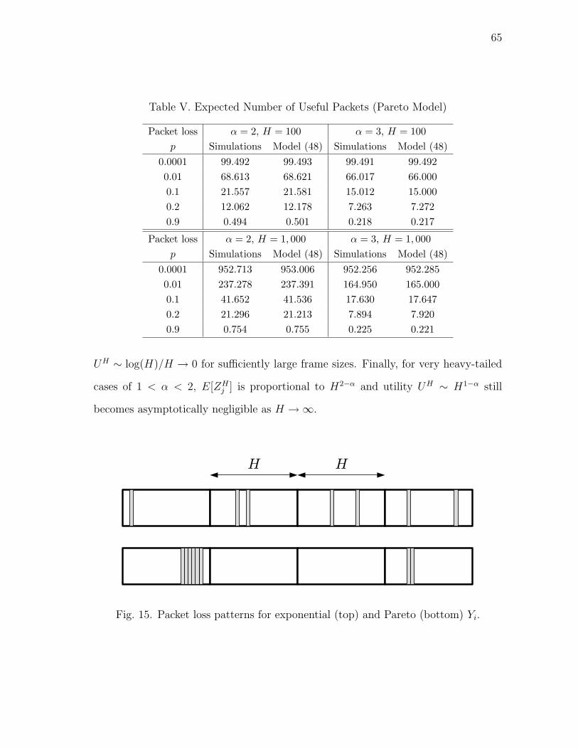
65

Table V. Expected Number of Useful Packets (Pareto Model)

Packet loss α = 2, H = 100 α = 3, H = 100p Simulations Model (48) Simulations Model (48)

0.0001 99.492 99.493 99.491 99.4920.01 68.613 68.621 66.017 66.0000.1 21.557 21.581 15.012 15.0000.2 12.062 12.178 7.263 7.2720.9 0.494 0.501 0.218 0.217

Packet loss α = 2, H = 1, 000 α = 3, H = 1, 000p Simulations Model (48) Simulations Model (48)

0.0001 952.713 953.006 952.256 952.2850.01 237.278 237.391 164.950 165.0000.1 41.652 41.536 17.630 17.6470.2 21.296 21.213 7.894 7.9200.9 0.754 0.755 0.225 0.221

UH ∼ log(H)/H → 0 for sufficiently large frame sizes. Finally, for very heavy-tailed

cases of 1 < α < 2, E[ZHj ] is proportional to H2−α and utility UH ∼ H1−α still

becomes asymptotically negligible as H →∞.

H H

Fig. 15. Packet loss patterns for exponential (top) and Pareto (bottom) Yi.

66

3. Discussion

Note that for many Internet applications and protocols (such as TCP), it is typically

understood that uniform packet loss has benefits over bursty loss. Interestingly, how-

ever, our results imply that for streaming of embedded video signals, bursty packet

drops are more desirable than uniformly random. It is further important to note that

video-coding methods that use error concealment may exhibit lower performance un-

der bursty loss, in which case the above conclusions would not necessarily hold. In

all other cases, subsequent losses within a given frame have no effect on the already-

useless frame data and thus lead to better performance of the application as they

allow a larger portion of the remaining frames to be loss-free.

We next investigate FEC-based streaming as an alternative to retransmission.

We study the characteristics of packet drops in an FEC-block in the following section

and discuss the impact of loss on FEC-protected video in Section D.

C. Impact of Packet Loss on FEC

The distribution of the number of lost packets and the location of the first loss in a

block play an important role in understanding the effectiveness of FEC. This section

studies these two metrics and offers a model for each assuming large sending rates.

We start by briefly discussing previous work on Markov loss models and pointing

out their shortcomings.

1. Background

The original work by Gilbert [32] examines loss events in communication channels

under a two-state Markov chain and provides an error model based on recursive

formulas that compute the probability of losing a certain number of packets in a

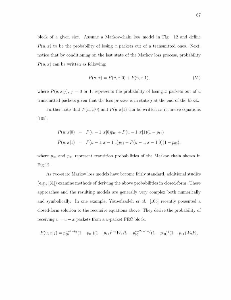
67

block of a given size. Assume a Markov-chain loss model in Fig. 12 and define

P (u, x) to be the probability of losing x packets out of u transmitted ones. Next,

notice that by conditioning on the last state of the Markov loss process, probability

P (u, x) can be written as following:

P (u, x) = P (u, x|0) + P (u, x|1), (51)

where P (u, x|j), j = 0 or 1, represents the probability of losing x packets out of u

transmitted packets given that the loss process is in state j at the end of the block.

Further note that P (u, x|0) and P (u, x|1) can be written as recursive equations

[105]:

P (u, x|0) = P (u− 1, x|0)p00 + P (u− 1, x|1)(1− p11)

P (u, x|1) = P (u− 1, x− 1|1)p11 + P (u− 1, x− 1|0)(1− p00),

where p00 and p11 represent transition probabilities of the Markov chain shown in

Fig.12.

As two-state Markov loss models have become fairly standard, additional studies

(e.g., [31]) examine methods of deriving the above probabilities in closed-form. These

approaches and the resulting models are generally very complex both numerically

and symbolically. In one example, Yousefizadeh et al. [105] recently presented a

closed-form solution to the recursive equations above. They derive the probability of

receiving v = u− x packets from a u-packet FEC block:

P (u, x|j) = pu−2x+j00 (1− p00)(1− p11)

1−jW1P0 + pu−2x−1+j00 (1− p00)

j(1− p11)W2P1,

68

where

W1 =x−1∑i=0

(x− 1

i

)(v

i + 1− j

)(p00p11)

x−1−i((1− p00)(1− p11)

)i

,

W2 =

x−j∑i=0

(x

i + j

)(v − 1

i

)(p00p11)

x−i−j((1− p00)(1− p11)

)i

.

Note that this model holds only for particular conditions (such as u ≥ 2x + 1)

and is computationally intensive for non-trivial u even though it does not require

solving recursive equations. Also note that none of the previous models provides

explicit information about the distribution of the number of lost packets per block or

the location of the first loss event.

In the following subsections, we examine a new (asymptotic) methodology that

computes the probability P (u, x) and related metrics of interest in simple closed-form

terms.

2. Basic Model

To investigate how the Markov loss process affects each block of FEC, we define L(n)

to be the random number of packets lost in a given block of size n ≥ 1. Notice that

P (u, x) discussed in the previous subsection is simply P (L(u) = x). Next, define

Bernoulli random variables:

Xi =

1 packet i is lost

0 otherwise

, 1 ≤ i ≤ n. (52)

where i is the sequence number of the packet within a given block of size n.

Then, the number of lost packets in the block is L(n) =∑n

i=1 Xi. Note, how-

ever, that since loss events Xi in the block are correlated under Markov loss, the

distribution of L(n) as n → ∞ does not follow the de Moivre-Laplace theorem for

69

independent random variables. Instead, L(n) converges to a Gaussian distribution

N(nE[Xi], V ar[∑

Xi]) as long as {Xi} are bounded and exhibit exponentially decay-

ing dependence5 [94]. In such cases, the approximation error is available explicitly

and is of the order of (log n)2/√

n. With this result in mind, normality of L(n) is

easy to establish and the only remaining pieces of the model are µ = E[L(n)] and

σ2 = V ar[L(n)], which we derive next.

3. Model Parameters

Assuming that the Markov chain is in the stationary state at the beginning of the

current block, we easily get:

µ = E[L(n)] = E[ n∑

i=1

Xi

]= np, (53)

which is the same result as in the de Moivre-Laplace theorem for sums of independent

variables [74]. Notice, however, that the variance of L(n) does not necessarily equal

the usual npq, where q = 1 − p. To understand the next result, define B to be the

transition matrix of the two-state Markov chain in (29):

B =

p00 1− p00

1− p11 p11

. (54)

Furthermore, denote by λ1 and λ2 the eigenvalues of the transition matrix B and

define a row vector v = (0, 1). Note that since for all stochastic matrices λ1 = 1, it is

easy to obtain that λ2 = p00 + p11 − 1. Then, we have the following lemma.

5In the context of Markov chains, this means that the chain changes its state withnon-zero probability (i.e., p00 ≥ ε, p11 ≥ ε for some ε > 0) (see Theorem 8.9 in [8]).

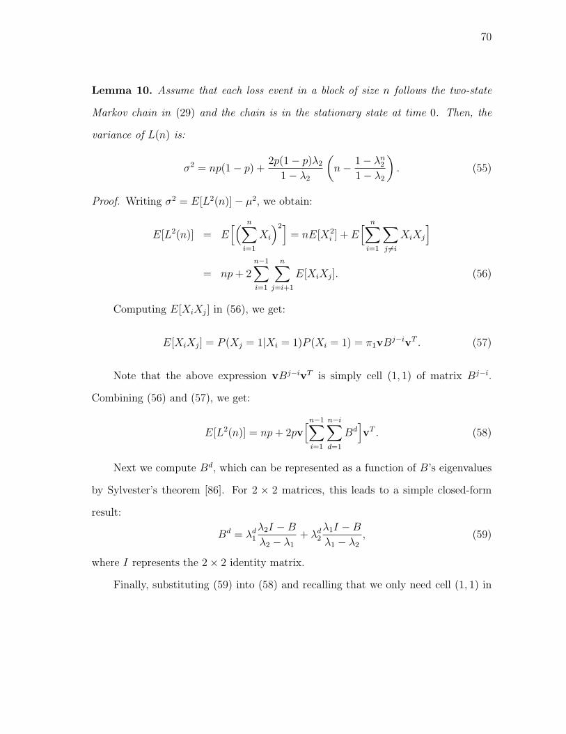
70

Lemma 10. Assume that each loss event in a block of size n follows the two-state

Markov chain in (29) and the chain is in the stationary state at time 0. Then, the

variance of L(n) is:

σ2 = np(1− p) +2p(1− p)λ2

1− λ2

(n− 1− λn

2

1− λ2

). (55)

Proof. Writing σ2 = E[L2(n)]− µ2, we obtain:

E[L2(n)] = E[( n∑

i=1

Xi

)2]= nE[X2

i ] + E[ n∑

i=1

∑

j 6=i

XiXj

]

= np + 2n−1∑i=1

n∑j=i+1

E[XiXj]. (56)

Computing E[XiXj] in (56), we get:

E[XiXj] = P (Xj = 1|Xi = 1)P (Xi = 1) = π1vBj−ivT . (57)

Note that the above expression vBj−ivT is simply cell (1, 1) of matrix Bj−i.

Combining (56) and (57), we get:

E[L2(n)] = np + 2pv[n−1∑

i=1

n−i∑

d=1

Bd]vT . (58)

Next we compute Bd, which can be represented as a function of B’s eigenvalues

by Sylvester’s theorem [86]. For 2 × 2 matrices, this leads to a simple closed-form

result:

Bd = λd1

λ2I −B

λ2 − λ1

+ λd2

λ1I −B

λ1 − λ2

, (59)

where I represents the 2× 2 identity matrix.

Finally, substituting (59) into (58) and recalling that we only need cell (1, 1) in

71

Bd, we get:

E[L2(n)] = np + 2pn−1∑i=1

n−i∑

d=1

[p + (1− p)λd2] = np + 2p

[pn(n− 1)

2+ R(n)

], (60)

where

R(n) =(1− p)λ2

1− λ2

(n− 1− λn

2

1− λ2

). (61)

Combining (53), (60), and (61), we get (55).

Simulations confirm that (55) is exact (for examples, see the table on page 75).

4. Asymptotic Approximation

In this subsection, we examine asymptotic (i.e., for large6 n) characteristics of the

distribution of L(n). Note that unless 2− p00 − p11 = 1− λ2 is on the order of 1/n,

the term λn2 in (55) is virtually zero for non-trivial n À 1. Since p is fixed and B

cannot depend on n, we can drop λn2 in (61) to obtain:

R(n) ≈ (1− p)λ2

1− λ2

(n− 1

1− λ2

). (62)

This leads to the following approximation on σ2 = np(1− p) + 2pR(n) for large

n:

σ2 ≈ np(1− p) +2p(1− p)λ2

1− λ2

(n− 1

1− λ2

). (63)

Notice that when R(n)/n ≈ 0, the model above simplifies to the case of Bernoulli

loss and σ2 reduces to npq(1 + o(1)). Thus, term R(n) determines the amount of

“dependency” in the sequence and the amount of deviation of σ2 from its uncorrelated

version. For convenience, re-write (63) as:

σ2 = np(1− p)

(1 +

2λ2

1− λ2

[1− 1

(1− λ2)n

]). (64)

6Throughout the chapter, “asymptotically large n” means that np À 0.

72

As a result of this transformation, it is easy to observe as a self-check that σ2 ≈npq when λ2 ≈ 0 (or p00 + p11 ≈ 1), or in other words, when there is no dependency

between Xi and Xj. This indeed reduces the Markov-chain to the Bernoulli case and

allows the de Moivre-Laplace theorem to hold.

For large np, we can state that for 2− p00 − p11 ≥ ε > 0:

limn→∞

σ2

n= p(1− p)

(1 +

2λ2

1− λ2

). (65)

Combining the above discussion into a single approximation, we obtain the fol-

lowing distribution of L(n).

Corollary 5. Assume that each loss event in a block of size n follows the two-state

Markov chain in (29), the chain is in the stationary state at time 0, and 2−p00−p11 ≥ε > 0. Then, the distribution of L(n) for large n is:

L(n) ∼ N

(np, np(1− p)

p00 + p11

2− p00 − p11

). (66)

Next, we verify model (66) using Matlab simulations. We create a Markov process

using two different values of p with two sets of transition probabilities (p00, p11). We

use p00 = 0.4, p11 = 0.1 to obtain large packet loss p = 0.4 and p00 = 0.92, p11 = 0.28

for smaller packet loss p = 0.1. Simulation results are compared to the model in Fig.

16, where the curve “Gaussian model” is the standard distribution N(np, npq) for

independent loss events and curve “our model” represents the distribution predicted

by (66). As the figure shows, model (66) matches the simulation very well, while

the classical Gaussian model exhibits variance inconsistent with that of the actual

distribution. Also notice in the figure that the true distribution of L(n) may have

σ2 both smaller and larger than the corresponding value npq. The first example has

p00 +p11 = 0.5, which results in σ2 ≈ npq/3. The second example has p00 +p11 = 1.2,

73

130 140 150 160 170 180 1900

0.02

0.04

0.06

0.08

0.1

Number of lost packets L

PM

FsimulationsGaussian modelour model

(a) p = 0.4

10 20 30 40 50 60 700

0.02

0.04

0.06

0.08

0.1


PM

F

simulationsGaussian modelour model

(b) p = 0.1

Fig. 16. Distribution of L(n) for n = 400 and two different p.

which leads to σ2 = 1.5npq. Further note that (66) holds for relatively small n as

well. Fig. 17 shows two examples for n = 50 and n = 20, respectively, where the

match is just as good as in Fig. 16.

Numerical assessment of the model is shown in Table VI, which illustrates several

examples from the CDF tail of both distributions in Fig. 17. As the table shows, for

both values of n, (66) matches simulations very well.

5. Non-Stationary Initial State

We now tackle the issue of non-stationary initial distribution of X0, which is the

state of the packet preceding the first packet in the FEC block. This analysis will

be required later for the derivation of streaming utility UH . Define Lc(n) to be the

random number of packets lost in a given block of size n conditioned on the initial

state X0 being 1 and µc to be its mean:

µc = E[Lc(n)] = E[L(n)|X0 = 1]. (67)

74

10 15 20 25 300

0.05

0.1

0.15

0.2

0.25


PM

F


(a) n = 50

0 5 10 150

0.1

0.2

0.3

0.4


PM

F


(b) n = 20

Fig. 17. Distribution of L(n) for p = 0.4 (p00 = 0.4, p11 = 0.1).

Lemma 11. Assume that each loss event in a block of length n follows the two-state

Markov chain in (29). Then, the mean of Lc(n) for large n is:

µc = np + (1− p)λ21− λn

2

1− λ2

. (68)

Proof. Note that the mean of L(n) conditioned on the value of initial state X0 = x

is:

E[L(n)|X0 = x] =n∑

i=1

P (Xi = 1|X0 = x). (69)

To obtain P (Xi = 1|X0 = x), we need cell (x, 1) from the matrix Bi. From (59),

we easily establish that:

P (Xi = 1|X0 = x) =

π1(1− λi2) x = 0

π1 + (1− π1)λi2 x = 1

. (70)

Setting x = 1 and expanding (69) using (70), we get (68).

Simulations confirm that (68) is exact. For large n, the term λn2 becomes negli-

75

Table VI. Comparison of (66) to Simulations (p = 0.4)

n Metric Simulations Model (66) Gaussian model50 µ 20.000 20.000 20.000

σ2 4.106 4.106 12.000P (L(n) ≤ 16) 0.043 0.042 0.156P (L(n) ≤ 24) 0.989 0.986 0.903

20 µ 8.000 8.000 8.000σ2 1.706 1.706 4.800

P (L(n) ≤ 6) 0.121 0.125 0.246P (L(n) ≤ 10) 0.979 0.972 0.873

gible and thus (68) can be simplified to:

µc ≈ np +λ2(1− p)

1− λ2

. (71)

Next, define σ2c to be the variance of Lc(n):

σ2c = V ar[Lc(n)] = V ar[L(n)|X0 = 1]. (72)

Then, we have the following result.

Lemma 12. Assume that each loss event in a block of length n follows the two-state

Markov chain in (29). Then, the variance of Lc(n) for large n is:

σ2c ≈ (p− 1)

[np + p +

1− 2np− 6p

γ+

5p− 1

γ2

], (73)

where γ = 2− p00 − p11 ≥ ε > 0.

Proof. Write the conditional variance σ2c as:

σ2c = E[L2(n)|X0 = 1]− µ2

c . (74)

76

Then, we can express the first term of (74) as:

E[L2(n)|X0 = 1] = E[L(n)|X0 = 1] + 2n−1∑i=1

n∑j=i+1

E[XiXj|X0 = 1]. (75)

Notice that by conditioning on X0 = x, E[XiXj] depends on the value of i in

addition to the distance d = j − i:

E[XiXj|X0 = x] = vBdvT P (Xi = 1|X0 = x). (76)

Using (76) and (70), we obtain:

E[XiXj|X0 = 1] = (p + (1− p)λj−i2 )(p + (1− p)λi

2). (77)

Denoting by G the double summation term in (75) and expanding it using (77),

we have:

G =n−1∑i=1

n∑j=i+1

E[XiXj|X0 = 1] (78)

=n−1∑j=1

(p2j − p + p2 + p(1− p)

1− λj+12

1− λ2

)

+n−1∑j=1

((p2 − p)jλj

2 −(1− p)2

1− λ2

λn+12

)

+n−1∑j=1

(np(1− p)− (1− p)2 +

(1− p)2

1− λ2

)λj

2.

Let G1, G2, and G3 be the first, second, and third summations in (78), respec-

tively. Expanding each term separately, we get:

G1 = (n− 1)

(p2n

2− p + p2 +

p(1− p)

1− λ2

)− p(1− p)λ2

2(1− λn−12 )

(1− λ2)2,

G2 = (p2 − p)λ2(1− nλn−1

2 )(1− λ2) + λ2(1− λn−12 )

(1− λ2)2− (1− p)2

1− λ2

(n− 1)λn+12 ,

G3 =

((1− p)(np− 1 + p) +

(1− p)2

1− λ2

)λ2(1− λn−1

2 )

1− λ2

.

77

130 140 150 160 170 180 1900

0.02

0.04

0.06

0.08

0.1


PM

Fsimulationsour model

(a) p = 0.4

0 20 40 60 800

0.02

0.04

0.06

0.08


PM

F

simulationsour model

(b) p = 0.1

Fig. 18. Distribution of Lc(n) for n = 400 and two different p.

Using the same argument for large n as in the previous subsection and dropping

terms λn−12 and λn+1

2 , we can simplify G1, G2, and G3 to:

G1 = (n− 1)

(p2n

2− p + p2 +

p(1− p)

1− λ2

)− p(1− p)λ2

2

(1− λ2)2,

G2 =(p2 − p)λ2

1− λ2

(1 +

λ2

1− λ2

), (79)

G3 =

((1− p)(np− 1 + p) +

(1− p)2

1− λ2

)λ2

1− λ2

.

Substituting λ2 = p00 + p11 − 1 and using (71) and (79), we obtain (73).

Combining (68) and (73), the next asymptotic result follows immediately.

Corollary 6. Assume that each loss event in a block of length n follows the two-state

Markov chain in (29). Then, the distribution of Lc(n) for large n is:

Lc(n) ∼ N(µc, σ2c ). (80)

We next present simulations that show the accuracy of (80). For this example,

we use n = 400 and two different values of p and plot the distribution of Lc(n) in Fig.

78

Table VII. Comparison of (80) to Simulations (p = 0.4)

n Metric Simulations Model (80)400 µc 159.800 159.800

σ2c 32.053 32.053

P (Lc(n) ≤ 142) 0.001 0.001P (Lc(n) ≤ 150) 0.051 0.050P (Lc(n) ≤ 170) 0.971 0.970

18. To demonstrate the numerical match, we compute several metrics of interest for

p = 0.4 and compare them with (80) in Table VII. As the figure and table show, (80)

agrees with simulations very well.

D. Performance of FEC in Scalable Streaming

Our next step is to study the performance of FEC-based video streaming considering

two loss patterns and analyze the convergence point of UH as H →∞.

Since our main interest in FEC is how its overhead affects the utility of received

video, we examine a generic media-independent FEC scheme based on (n, k) block

codes (such as parity or Reed-Solomon codes), where n is the total number of packets

in an FEC block and k is the number of redundant FEC packets in the block. Thus,

the actual number of video data packets in each block is H = n − k and the FEC

overhead rate (i.e., fraction of FEC packets) ψ is k/n. Recall that under (n, k) block

coding, all H data packets are recovered if the number of lost packets in a block is

no more than the number of FEC packets k. However, if the channel loses more than

k packets, then only those packets in the enhancement layer located before the first

loss in the block can be used in decoding.

79

1. Markov Packet Loss

In this subsection, we first investigate the expected amount of data recovered in each

block and in the next subsection analyze the corresponding utility of received video.

To derive E[ZHj ], we again assume that L(n) is the number of packets lost in a

block of size n and define Q = E[ZHj | L(n) > k] to be the expected number of useful

video packets recovered from an FEC block when L(n) is greater than the number of

FEC packets in the block. The following result states the value of Q.

Lemma 13. Assuming a two-state Markov packet loss in (29) and L(n) > k, the

expected number of useful video packets recovered per frame is:

Q = E[ZHj | L(n) > k] =

p00p11 − λ2

1− λ2

n−k−1∑i=1

ipi−100

P (Lc(n− i− 1) > k − 1)

P (L(n) > k). (81)

Proof. Assume that Dj is the random distance in packets to the first loss in a block

j as before. Then, we can obtain P (Dj = i) using the basic properties of Markov

chains:

P (Dj = i) =

π1 i = 0

π0pi−100 (1− p00) i ≥ 1

. (82)

Next, write Q as:

Q = E[ZHj |L(n) > k] =

n−k−1∑i=1

iP (Dj = i|L(n) > k).

Using Bayes’ formula, we can get:

P (Dj = i|L(n) > k) =P (L(n) > k|Dj = i)P (Dj = i)

P (L(n) > k). (83)

Next note that we can compute:

P (L(n) > k|Dj = i) = P (Lc(n− i− 1) > k − 1), (84)

80

Table VIII. Comparison of (81) to Simulations

p = 0.4, n = 400, σ2 = 32.106k P (L(n) > k) Q in simulations Q in (81)

170 0.0307 0.802 0.807165 0.1656 0.863 0.865160 0.4674 0.919 0.920155 0.7874 0.964 0.963140 0.9996 0.999 0.9990 1.0000 1.000 1.000

p = 0.1, n = 400, σ2 = 54.943k P (L(n) > k) Q in simulations Q in (81)50 0.0809 8.245 8.00245 0.2224 8.905 8.80040 0.4593 9.604 9.60130 0.9068 10.813 10.84020 0.9983 11.231 11.2240 1.0000 11.250 11.250

which represents the probability of losing more than k − 1 packets from n − i − 1

transmitted ones conditioned on the (i + 1)-st packet being lost.

Finally, recalling that π0 = (1 − p11)/(2 − p00 − p11) = (1 − p11)/(1 − λ2) and

with the help of (83), (84), and (82), we get (81).

Notice that by utilizing the models derived in section C., we can compute for

asymptotically large n each of the terms in (81) individually, which in turn allows us

to calculate Q. To verify (81), we compute Q in simulations and show the result in

Table VIII. For the first case, we use large packet loss p = 0.4 (p00 = 0.4, p11 = 0.1),

n = 400, and over 1 billion iterations. As the table shows, (81) matches simulation

results very well. For the second case, we use smaller packet loss p = 0.1 (p00 = 0.92,

p11 = 0.28) and observe in the table that (81) is reasonably accurate as well. It is

worth noting that the model is more accurate when np is large or σ2 < np. Thus,

81

due to the small np and σ2 > np, the match in the second case in Table VIII is not

as good as that in the first case.

Using the result in (81), we easily get E[ZHj ].

Corollary 7. Assuming two-state Markov packet loss with average loss probability p,

the expected number of useful packets recovered per FEC block of size n is:

E[ZHj ] = P (L(n) ≤ k)H + P (L(n) > k)Q. (85)

2. Utility

Defining a new metric C(n) = QP (L(n) > k) and re-writing (28) using (85), we get:

UH =P (L(n) ≤ k)H + C(n)

n(1− p). (86)

For convenience of presentation, define the overhead rate ψ as a linear function

of packet loss: ψ = ηp (where η is a constant). Then, we have in the next theorem

the asymptotic behavior of UH as the video rate becomes large.

Theorem 8. Assuming a two-state Markov packet loss in an FEC block of size n,

average loss probability p, and FEC overhead rate ψ = ηp, (0 < ψ < 1), the utility of

received video for each FEC block converges to the following:

limH→∞

UH =

0 0 < η < 1

0.5 η = 1

1− ψ

1− p1 < η < 1/p

. (87)

Proof. Recalling that the distribution of L(n) is asymptotically normal with param-

82

eters µ and σ2 as discussed in Section C.4, we can write:

P (L(n) ≤ k) =

k∫

−∞

f(x)dx, (88)

where f(x) is the PDF of L(n).

Define φ(x) to be the PDF of the standard normal distribution and let z =

(k − µ)/σ. Then, re-write (88) as:

P (L(n) ≤ k) =

z∫

−∞

φ(x)dx. (89)

Using ψ = ηp and k = ψn, re-write z as:

z =(η − 1)

√(H + k)p√

(1− p)p00 + p11

2− p00 − p11

. (90)

Notice that (p00 +p11)/(2−p00−p11) > 0 and observe from (90) that as H →∞,

z → −∞ if η < 1, z → ∞ if η > 1, and z = 0 if η = 1. Thus, the probability

P (L(n) ≤ k) in (89) converges to the following as H →∞:

limH→∞

P (L(n) ≤ k) =

0 0 < η < 1

0.5 η = 1

1 1 < η < 1/p

. (91)

Next, observe in (81) that since P (Lc(n− i− 1) > k− 1) is less than or equal to

1, C(n) is upper-bounded by:

C(n) ≤ p00p11 − λ2

1− λ2

n−k−1∑i=1

ipi−100 =

p00p11 − λ2

1− λ2

C, (92)

where

C =n−k−1∑

i=1

ipi−100 . (93)

83

500 1000 15000

0.2

0.4

0.6

0.8

1

η=1.2

η=1.0

η=0.8

Frame size H

Util

ity

ModelSimulation

(a) Bernoulli loss

500 1000 15000

0.2

0.4

0.6

0.8

1

h=1.2

h=1.0

h=0.8

Frame size H

Utilit

y

ModelSimulation

(b) Markov loss

Fig. 19. Simulation results of UH and their comparison to model (87) for Bernoulli

loss and Markov loss (p00 = 0.92, p11 = 0.28). In both figures, p = 0.1.

Recalling that p00 > 0 and expanding (93), we get:

C =1 + (n− k − 1)pn−k

00 − (n− k)pn−k−100

(1− p00)2. (94)

Since C/n → 0 as n → ∞, so does C(n)/n. Thus, using (91) in (86), and

utilizing the fact that H = n(1− ψ), we immediately get (87).

We next verify the asymptotic characteristics of the achieved utility in (87).

Before considering a general Markov loss model, we first examine a special case with

p00 = 1−p (i.e., Bernoulli loss). Fig. 19(a) plots simulation results of UH for different

η and compare them with (87). As the figure shows, (87) matches simulations very

well and UH indeed converges to 0, 0.5 or (1− ψ)/(1− p) = 0.9778 as the streaming

rate becomes high. For the general Markov loss case, we plot simulation results UH

and compare them with the values predicted by (87) for three different values of η in

Fig. 19(b). As the figure shows, UH follows a trend similar to that in the Bernoulli

case with the exception of a slightly slower convergence rate (Markov chains with

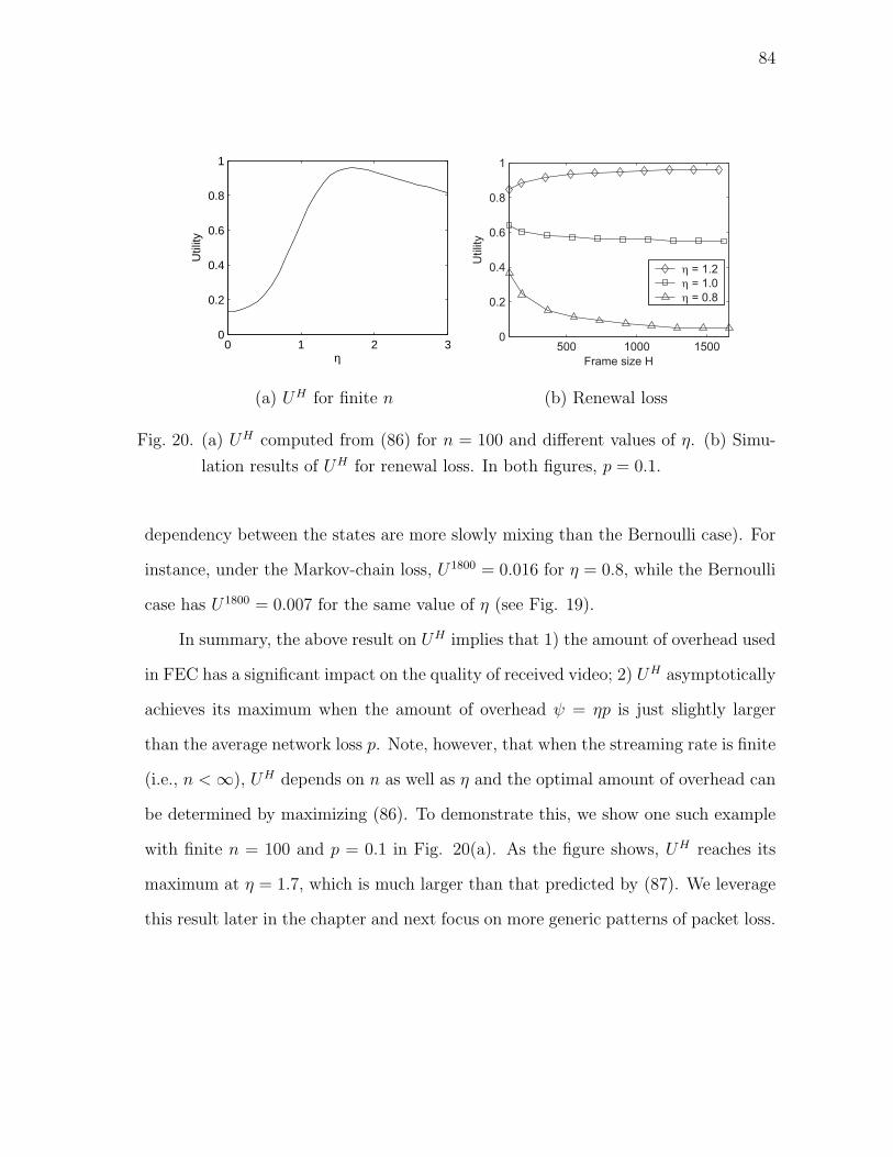
84

0 1 2 30

0.2

0.4

0.6

0.8

1

η

Util

ity

(a) UH for finite n

500 1000 15000

0.2

0.4

0.6

0.8

1

Frame size H

Utilit

y

h = 1.2

h = 1.0

h = 0.8

(b) Renewal loss

Fig. 20. (a) UH computed from (86) for n = 100 and different values of η. (b) Simu-

lation results of UH for renewal loss. In both figures, p = 0.1.

dependency between the states are more slowly mixing than the Bernoulli case). For

instance, under the Markov-chain loss, U1800 = 0.016 for η = 0.8, while the Bernoulli

case has U1800 = 0.007 for the same value of η (see Fig. 19).

In summary, the above result on UH implies that 1) the amount of overhead used

in FEC has a significant impact on the quality of received video; 2) UH asymptotically

achieves its maximum when the amount of overhead ψ = ηp is just slightly larger

than the average network loss p. Note, however, that when the streaming rate is finite

(i.e., n < ∞), UH depends on n as well as η and the optimal amount of overhead can

be determined by maximizing (86). To demonstrate this, we show one such example

with finite n = 100 and p = 0.1 in Fig. 20(a). As the figure shows, UH reaches its

maximum at η = 1.7, which is much larger than that predicted by (87). We leverage

this result later in the chapter and next focus on more generic patterns of packet loss.

85

3. Renewal Packet Loss

In this section, we study UH under ON/OFF renewal packet loss. Similarly to the

result in (85) discussed in Section D.1, we model the amount of useful data recovered

from an FEC block as:

E[ZHj ] = E[ZH

j |L(t) ≤ k]P (L(t) ≤ k) + E[ZHj |L(t) > k]P (L(t) > k), (95)

where L(t) =∫ t+n

tV (u)du is the number of lost packets in a block of size n starting

at time instant t and V (u) is the ON/OFF process described in Section B.2. Un-

fortunately, computing distribution P (L(t) ≤ k) under an ON/OFF renewal process

appears to be impossible in closed form even though many studies (e.g., [97]) have at-

tempted this task in the last 50 years. Hence, we do not pursue this direction further

and show instead convergence of UH using simulations without offering a closed-form

model.

For this case, we generate 20 million random values for ON and OFF durations,

where each of Xi and Yi are i.i.d. Pareto. We use E[Yi] = 10 and E[Xi] = E[Yi]p/(1−p) so as to keep the average loss equal to p and plot the simulation results of UH for

different values of η and p = 0.1 in Fig. 20(b). As the figure shows, UH again exhibits

a percolation point around η = 1 (i.e., ψ = p) and converges to three different values

depending on η.

The final question we address is whether UH converges to the same values as in

the Markov case. We conduct simulations using very large n and several values of p.

For each value of p, we identify a convergence point, at which increasing H virtually

does not change the value of UH (change in UH after doubling the value of H is less

than 0.001) and illustrate in Table IX convergence values of UH for η = 1.2. As the

table shows, UH approaches to (1−ψ)/(1−p) regardless of the value of p. This is the

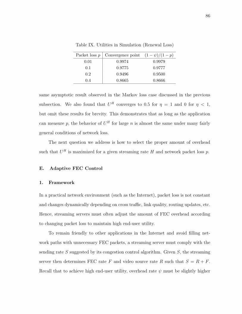
86

Table IX. Utilities in Simulation (Renewal Loss)

Packet loss p Convergence point (1− ψ)/(1− p)0.01 0.9974 0.99790.1 0.9775 0.97770.2 0.9496 0.95000.4 0.8665 0.8666

same asymptotic result observed in the Markov loss case discussed in the previous

subsection. We also found that UH converges to 0.5 for η = 1 and 0 for η < 1,

but omit these results for brevity. This demonstrates that as long as the application

can measure p, the behavior of UH for large n is almost the same under many fairly

general conditions of network loss.

The next question we address is how to select the proper amount of overhead

such that UH is maximized for a given streaming rate H and network packet loss p.

E. Adaptive FEC Control

1. Framework

In a practical network environment (such as the Internet), packet loss is not constant

and changes dynamically depending on cross traffic, link quality, routing updates, etc.

Hence, streaming servers must often adjust the amount of FEC overhead according

to changing packet loss to maintain high end-user utility.

To remain friendly to other applications in the Internet and avoid filling net-

work paths with unnecessary FEC packets, a streaming server must comply with the

sending rate S suggested by its congestion control algorithm. Given S, the streaming

server then determines FEC rate F and video source rate R such that S = R + F .

Recall that to achieve high end-user utility, overhead rate ψ must be slightly higher

87

than packet loss p as discussed in Section D; however, the exact value of optimal

ψ∗ depends on the streaming rate and current packet loss p (the latter of which is

generally coupled with congestion control and should be provided by its feedback

loop).

Next, we discuss a simple approach that can select the proper amount of FEC

overhead using our previous analysis. The main problem is how to select optimal

η∗ for a given packet loss p and FEC block size n to achieve maximum utility. One

simple solution is to construct an optimization problem around (86):

η∗ = arg maxη

UH(η, p, n), (96)

which can be easily solved using binary search and applying models developed in the

previous section as long as packet loss p, block size n, and Markov properties of the loss

process are known. In practice, this can be implemented by fitting a Markov model

to the measured loss events and maximizing utility in (96) regardless of whether the

actual network loss exhibits Markovian properties or not. Simulations below suggest

that the actual distribution of loss-burst lengths does not have a significant effect on

the result.

2. Evaluation Setup

In this section, we present simulation results of our adaptive FEC-based scheme

including the properties of UH and video quality. We first simulate a Markov loss

process, obtain packet loss statistics for each video frame, and examine the resulting

utility and PSNR video quality of our method in comparison to two approaches

that use fixed amounts of FEC overhead. We then conduct ns2 [73] simulations to

briefly investigate whether the results obtained from the Markov model are valid in

more realistic network environments. In all simulations, one video frame (40, 000

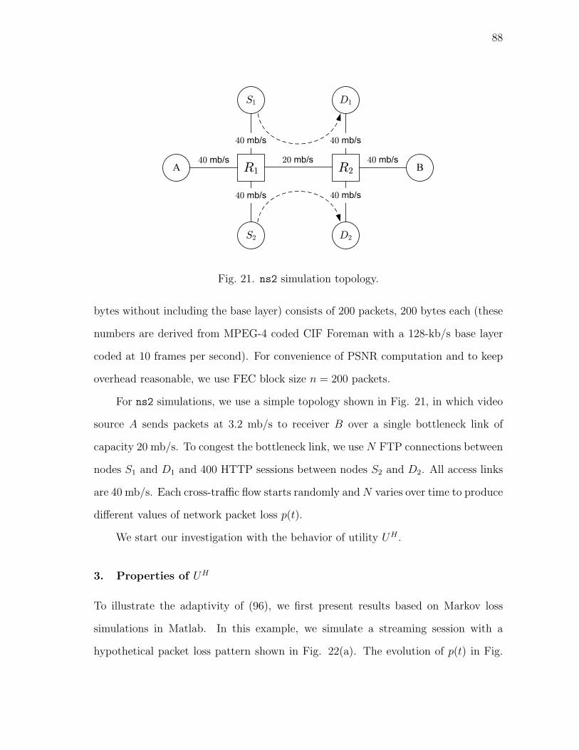
88

R1 R2A B

S1

S2

D1

D2

20 mb/s40 mb/s 40 mb/s

40 mb/s 40 mb/s

40 mb/s 40 mb/s

Fig. 21. ns2 simulation topology.

bytes without including the base layer) consists of 200 packets, 200 bytes each (these

numbers are derived from MPEG-4 coded CIF Foreman with a 128-kb/s base layer

coded at 10 frames per second). For convenience of PSNR computation and to keep

overhead reasonable, we use FEC block size n = 200 packets.

For ns2 simulations, we use a simple topology shown in Fig. 21, in which video

source A sends packets at 3.2 mb/s to receiver B over a single bottleneck link of

capacity 20 mb/s. To congest the bottleneck link, we use N FTP connections between

nodes S1 and D1 and 400 HTTP sessions between nodes S2 and D2. All access links

are 40 mb/s. Each cross-traffic flow starts randomly and N varies over time to produce

different values of network packet loss p(t).

We start our investigation with the behavior of utility UH .

3. Properties of UH

To illustrate the adaptivity of (96), we first present results based on Markov loss

simulations in Matlab. In this example, we simulate a streaming session with a

hypothetical packet loss pattern shown in Fig. 22(a). The evolution of p(t) in Fig.

89

0 20 40 60 80 1000

0.1

0.2

0.3

0.4

0.5

Control intervals

Pac

ket l

oss

(a) Packet loss pattern

0 20 40 60 80 1000.2

0.4

0.6

0.8

1

Control intervals

Tra

nsiti

on p

roba

bilit

y

p00

p11

(b) p00, p11

Fig. 22. Packet loss pattern obtained through Markov-chain simulation using transi-

tion probabilities p00 and p11.

22(a) is obtained using the Markov chain in (29) with transition probabilities p00 and

p11 plotted in Fig. 22(b). We consider two different fixed-overhead schemes (we call

them M1 and M2 hereafter) to compare with our adaptive method. To determine the

fixed amount of overhead, M1 and M2 use the lower (pL = 0.1) and upper (pU = 0.4)

bounds on packet loss in Fig. 22(a), respectively.

We plot the achieved utility of FEC-protected video in Fig. 23. As the figure

shows, (96) maintains its utility very high (in fact approaching the optimal value of

UH) along the entire streaming session with small deviations only at points when p(t)

transitions to its new value. Also observe in the figure that fixed-overhead schemes

M1 and M2 perform much worse even though M2 sends more FEC than our scheme.

Next, we examine how (96) behaves under changing p(t) obtained from ns2 sim-

ulations. In this case, we vary the number of FTP connections N every 5 control

intervals and measure long-term average packet loss at the receiver. The relation-

ship between N and the long-term average loss is illustrated in Fig. 24(a) where

90

0 20 40 60 80 1000

0.2

0.4

0.6

0.8

1

1.2

Control intervals

Util

ityadaptiveM1

(a) pL = 0.1

0 20 40 60 80 1000

0.2

0.4

0.6

0.8

1

1.2

Control intervals

Util

ity

adaptiveM2

(b) pU = 0.4

Fig. 23. Metric UH achieved by the adaptive FEC overhead controller (96) and its com-

parison to utilities obtained in two different scenarios that use fixed amounts

of overhead.

the increase in packet loss is caused by the well-known TCP scalability properties

[20]. Changing the value of N randomly over time, the network exhibits fluctuating

packet loss shown in Fig. 24(b). Using this information, the sender estimates transi-

tion probabilities p00 and p11 for each interval and uses them in FEC control. Figs.

25(a) and 25(b) plot the evolution of UH achieved by different FEC-control schemes

and show that our adaptive controller exhibits behavior similar to that observed in

Markov-loss simulations.

Analysis in previous sections suggests that both correlated and uncorrelated loss

patterns, as well as exponential and heavy-tailed loss-burst lengths, lead to an almost

identical behavior of UH . Additional simulations with ns2 confirm that results based

on simple Markov-loss models can indeed be used as first-step approximations to the

real behavior of UH in generic networks. Future work will examine this issue in more

detail and attempt to understand how more complex loss patterns influence optimal

selection of FEC overhead.

91

100 200 300 400 500 6000

0.02

0.04

0.06

0.08

0.1

Number of FTP flows N

Ave

rage

pac

ket l

oss

rate

(a) Average loss rate

0 20 40 60 80 1000

0.02

0.04

0.06

0.08

0.1

0.12

Control intervals

Pac

ket l

oss

(b) Packet loss pattern

Fig. 24. (a) Average packet loss rate for different number of FTP flows N in ns2

simulation. (b) Packet loss pattern obtained through ns2 simulation.

0 20 40 60 80 1000

0.2

0.4

0.6

0.8

1

1.2

Control intervals

Util

ity

adaptiveM1

(a) pL = 0.01

0 20 40 60 80 1000

0.2

0.4

0.6

0.8

1

1.2

Control invervals

Util

ity

adaptiveM2

(b) pU = 0.1

Fig. 25. Evolution of UH achieved by the adaptive FEC overhead controller (96) and

its comparison to that of utilities obtained in two different scenarios that use

fixed amounts of overhead.

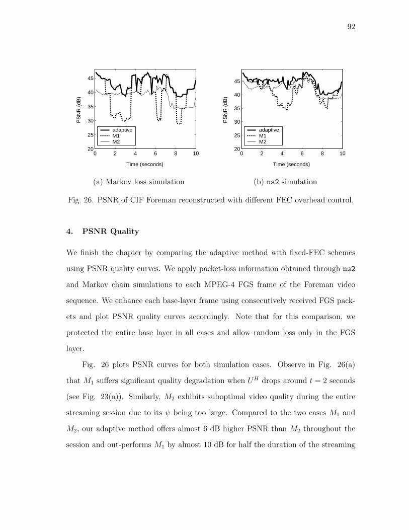
92

0 2 4 6 8 1020

25

30

35

40

45

Time (seconds)

PS

NR

(dB

)

adaptiveM1M2

(a) Markov loss simulation

0 2 4 6 8 1020

25

30

35

40

45

Time (seconds)

PS

NR

(dB

)

adaptiveM1M2

(b) ns2 simulation

Fig. 26. PSNR of CIF Foreman reconstructed with different FEC overhead control.

4. PSNR Quality

We finish the chapter by comparing the adaptive method with fixed-FEC schemes

using PSNR quality curves. We apply packet-loss information obtained through ns2

and Markov chain simulations to each MPEG-4 FGS frame of the Foreman video

sequence. We enhance each base-layer frame using consecutively received FGS pack-

ets and plot PSNR quality curves accordingly. Note that for this comparison, we

protected the entire base layer in all cases and allow random loss only in the FGS

layer.

Fig. 26 plots PSNR curves for both simulation cases. Observe in Fig. 26(a)

that M1 suffers significant quality degradation when UH drops around t = 2 seconds

(see Fig. 23(a)). Similarly, M2 exhibits suboptimal video quality during the entire

streaming session due to its ψ being too large. Compared to the two cases M1 and

M2, our adaptive method offers almost 6 dB higher PSNR than M2 throughout the

session and out-performs M1 by almost 10 dB for half the duration of the streaming

93

session.7 Fig. 26(b) shows that the improvement in ns2 simulations is not as dramatic

as that in the Markov example due to the lower packet loss rates, but nevertheless

amounts to a 3 to 9 dB improvement.

7Note that a 1-dB gain in PSNR is usually considered significant [100].

94

CHAPTER V

BANDWIDTH ESTIMATION: STOCHASTIC ANALYSIS

This chapter examines the problem of estimating the capacity and available band-

width of end-to-end paths under non-negligible cross-traffic conditions. In the first

half of this chapter, we present a stochastic analysis of the problem in the context

of a single congested node and derive several results that allow the construction of

asymptotically-accurate bandwidth estimators. We develop a generic queuing model

of an Internet router and propose a filtering solution that asymptotically converges

to the desired values of the bottleneck capacity and available bandwidth under ar-

bitrary (including non-stationary) cross-traffic. This is one of the first methods that

simultaneously estimates both types of bandwidth and is provably accurate. In the

second half, we focus on measuring both bandwidth metrics of the tight-link over a

multi-hop path using recursive extension of the single-hop model developed in the

first half. Using a new probing technique called Envelope based on the recursive

model, we develop an asymptotically accurate bandwidth estimator that optimally

selects probing parameters according to various network conditions and significantly

outperforms existing methods in terms of estimation accuracy.

A. Introduction

Bandwidth estimation has recently become an important and mature area of Internet

research [1], [2], [14], [22], [23], [35], [41], [43], [44], [52], [54], [55], [70], [72], [76],

[77], [78], [84], [85], [93], [96], [101]. A typical goal of these studies is to understand

the characteristics of Internet paths and those of cross-traffic through a variety of

95

end-to-end and/or router-assisted measurements. The proposed techniques usually

fall into two categories – those that estimate the bottleneck bandwidth [14], [22], [23],

[49] and those that deal with the available bandwidth [43], [72], [85], [96]. Recall that

the former bandwidth metric refers to the capacity of the slowest link of the path,

while the latter is generally defined as the smallest average unused bandwidth among

the routers of an end-to-end path.

The majority of existing bottleneck-bandwidth estimation methods are justi-

fied assuming no cross-traffic along the path and are usually examined in simula-

tions/experiments to show that they can work under realistic network conditions

[14], [22], [23], [35]. With available bandwidth estimation, cross-traffic is essential

and is usually taken into account in the analysis; however, such analysis predomi-

nantly assumes a fluid model for all flows and implicitly requires that such models

be accurate in non-fluid cases. Simulations/experiments are again used to verify that

the proposed methods are capable of dealing with bursty conditions of real Internet

cross-traffic [44], [72], [85], [96].

To understand some of the reasons for the lack of stochastic modeling in this

field, this work studies a single-node bandwidth measurement problem and derives a

closed-form estimator for both capacity C and available bandwidth A = C− r, where

r is the average rate of cross-traffic at the link. For an arbitrary cross-traffic arrival

process r(t), we define r as the asymptotic time-average of r(t) and assume that it

exists and is finite:

r = limt→∞

1

t

t∫

0

r(u)du < ∞. (97)

Notice that the existence of (97) does not require stationarity of cross-traffic,

nor does it impose any restrictions on the arrival of individual packets to the router.

While other definitions of available bandwidth A and the average cross-traffic rate

96

r are possible, we find that (97) serves our purpose well as it provides a clean and

mathematically tractable metric.

In this chapter, we first deals with bandwidth estimation under i.i.d. renewal

cross-traffic and the analysis of packet-pair/train methods. We first show that under

certain conditions and even the simplest i.i.d. cross-traffic, histogram-based methods

commonly used in prior work (e.g., [22]) can be misled into producing inaccurate

estimates of C. We overcome this limitation by developing an asymptotically accurate

model for C; however, since this approach eventually requires ergodicity of cross-

traffic, we later build another model that imposes more restriction on the sampling

process (using PASTA principles suggested in [96]), but allows cross-traffic to exhibit

arbitrary characteristics.

Unlike previous studies [96], we prove that the corresponding PASTA-based es-

timators converge to the correct values and show that they can be used to simulta-

neously measure capacity C and available bandwidth A. To our knowledge, this is

the first estimator that measures both C and A without congesting the link, assumes

non-negligible, non-fluid cross-traffic in the derivations, and applies to non-stationary

r(t).

B. Stochastic Queuing Model

In this section, we build a simple model of a router that introduces random delay

noise into the measurements of the receiver and use it to study the performance of

packet-pair bandwidth-sampling techniques. Note that we depart from the common

assumption of negligible and/or fluid cross-traffic and specifically aim to understand

the effects of random queuing delays on the bandwidth sampling process. First con-

sider an unloaded router with no cross-traffic. The packet-pair mechanism is based

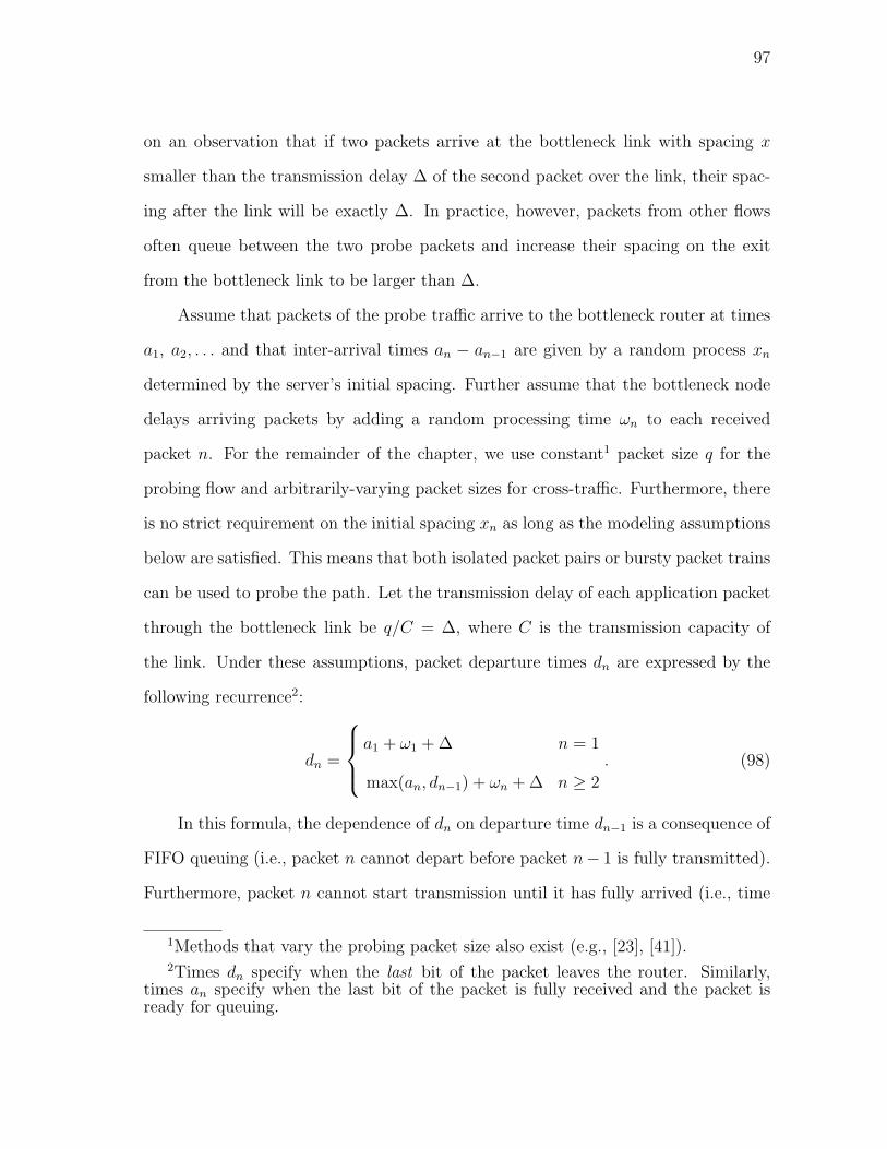
97

on an observation that if two packets arrive at the bottleneck link with spacing x

smaller than the transmission delay ∆ of the second packet over the link, their spac-

ing after the link will be exactly ∆. In practice, however, packets from other flows

often queue between the two probe packets and increase their spacing on the exit

from the bottleneck link to be larger than ∆.

Assume that packets of the probe traffic arrive to the bottleneck router at times

a1, a2, . . . and that inter-arrival times an − an−1 are given by a random process xn

determined by the server’s initial spacing. Further assume that the bottleneck node

delays arriving packets by adding a random processing time ωn to each received

packet n. For the remainder of the chapter, we use constant1 packet size q for the

probing flow and arbitrarily-varying packet sizes for cross-traffic. Furthermore, there

is no strict requirement on the initial spacing xn as long as the modeling assumptions

below are satisfied. This means that both isolated packet pairs or bursty packet trains

can be used to probe the path. Let the transmission delay of each application packet

through the bottleneck link be q/C = ∆, where C is the transmission capacity of

the link. Under these assumptions, packet departure times dn are expressed by the

following recurrence2:

dn =

a1 + ω1 + ∆ n = 1

max(an, dn−1) + ωn + ∆ n ≥ 2

. (98)

In this formula, the dependence of dn on departure time dn−1 is a consequence of

FIFO queuing (i.e., packet n cannot depart before packet n− 1 is fully transmitted).

Furthermore, packet n cannot start transmission until it has fully arrived (i.e., time

1Methods that vary the probing packet size also exist (e.g., [23], [41]).2Times dn specify when the last bit of the packet leaves the router. Similarly,

times an specify when the last bit of the packet is fully received and the packet isready for queuing.

98

n — 1

arrival

departure

n

a n — 1 an

y n time

n+1

y n+1

a n+1

xn xn+1

d n — 1 dn d n+1

n — 1 n n+1

Fig. 27. Departure delays introduced by the node.

an). The value of the noise term ωn is proportional to the number of packets generated

by cross-traffic and queued in front of packet n. The final metric of interest is inter-

departure delay yn = dn− dn−1 as the packets leave the router. The various variables

and packet arrival/departure are schematically shown in Figure 27.

Even though the model in (98) appears to be simple, it leads to fairly complicated

distributions for yn if we make no prior assumptions about cross-traffic. We next

examine several special cases and derive important asymptotic results about process

yn.

C. Renewal Cross-Traffic

1. Packet-Pair Analysis

We start our analysis with a rather common assumption in queuing theory that cross-

traffic arrives into the bottleneck link according to some renewal process (i.e., delays

between cross-traffic packets are i.i.d. random variables). In what follows in the next

few subsections, we show that modeling of this direction requires stationarity (more

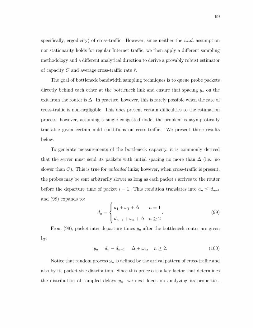
99

specifically, ergodicity) of cross-traffic. However, since neither the i.i.d. assumption

nor stationarity holds for regular Internet traffic, we then apply a different sampling

methodology and a different analytical direction to derive a provably robust estimator

of capacity C and average cross-traffic rate r.

The goal of bottleneck bandwidth sampling techniques is to queue probe packets

directly behind each other at the bottleneck link and ensure that spacing yn on the

exit from the router is ∆. In practice, however, this is rarely possible when the rate of

cross-traffic is non-negligible. This does present certain difficulties to the estimation

process; however, assuming a single congested node, the problem is asymptotically

tractable given certain mild conditions on cross-traffic. We present these results

below.

To generate measurements of the bottleneck capacity, it is commonly derived

that the server must send its packets with initial spacing no more than ∆ (i.e., no

slower than C). This is true for unloaded links; however, when cross-traffic is present,

the probes may be sent arbitrarily slower as long as each packet i arrives to the router

before the departure time of packet i − 1. This condition translates into an ≤ dn−1

and (98) expands to:

dn =

a1 + ω1 + ∆ n = 1

dn−1 + ωn + ∆ n ≥ 2

. (99)

From (99), packet inter-departure times yn after the bottleneck router are given

by:

yn = dn − dn−1 = ∆ + ωn, n ≥ 2. (100)

Notice that random process ωn is defined by the arrival pattern of cross-traffic and

also by its packet-size distribution. Since this process is a key factor that determines

the distribution of sampled delays yn, we next focus on analyzing its properties.

100

Assume that inter-packet delays of cross-traffic are given by independent random

variables {Xi} and the actual arrivals occur at times X1, X1 + X2, . . . Thus, the

arrival pattern of cross-traffic defines a renewal process M(t), which is the number of

packet arrivals in the interval [0, t]. Using common convention, further assume that

the mean inter-arrival delay E[Xi] is given by 1/λ, where λ = r is the mean arrival

rate of cross-traffic in packets per second.

To allow random packet sizes, assume that {Sj}, j = 1, 2, . . . are independent

random variables modeling the size of packets in cross-traffic. We further assume

that the bottleneck link is probed by a sequence of packet-pairs, in which the delay

between the packets within each pair is small (so as to keep their rate higher than

C) and the delay between the pairs is high (so as not to congest the link). Under

these assumptions, the amount of cross-traffic data received by the bottleneck link

between probe packets 2m − 1 and 2m (i.e., in the interval (a2m−1, a2m]) is given by

a cumulative reward process:

vn =

M(an)−M(an−1)∑j=1

Sj, n = 2m, (101)

where n represents the sequence number of the second packet in each pair. For now,

we assume a general (not necessarily equilibrium) process M(t) and re-write (100) as:

yn = ∆ +vn

C= ∆ +

M(an)−M(an−1)∑j=1

Sj

C, n = 2m. (102)

Since classical renewal theory is mostly concerned with limiting distributions, yn

by itself does not lead to any tractable results because the observation period of the

process captured by each of yn is very small.

101

Define a time-average process Wn to be the average of {yi} up to time n:

Wn =1

n

n∑i=1

yi. (103)

Then, we have the following result.

Theorem 9. Assuming ergodic cross-traffic, time-average process Wn converges to:

limn→∞

Wn = ∆ +λE[xn]E[Sj]

C= ∆ + E[ωn], (104)

where E[xn] is the mean inter-probe delay of packet-pairs.

Proof. Process Wn samples a much larger span of M(t) and has a limiting distribution

as we demonstrate below. Applying Wald’s equation to (102) [102]:

E [yn] = ∆ +E[M(an)−M(an−1)]E[Sj]

C. (105)

The last result holds since M(t) and Sj are independent and M(an)−M(an−1)

is a stopping time for sequence {Sj}. Equation (105) can be further simplified by

noticing that E[M(t)] is the renewal function m(t):

E [yn] = ∆ +(m(an)−m(an−1))E[Sj]

C. (106)

Assuming stationary cross-traffic, (106) expands to [102]:

E [yn] = ∆ +λE[xn]E[Sj]

C. (107)

Finally, assuming ergodicity of cross-traffic (which implies that of process yn),

we can obtain (107) using a large number of packet pairs as the limit of Wn in (103)

as n →∞.

Notice that the second term in (104) is strictly positive under the assumptions

of this work. This leads to an interesting observation that the filtering problem

102

we are facing is quite challenging since the sampled process yn represents signal ∆

corrupted by a non-zero-mean noise ωn. This is a drastic departure from the classical

filter theory, which mostly deals with zero-mean additive noise. It is also interesting

that the only way to make the noise zero-mean is to either send probe traffic with

E[xn] = 0 (i.e., infinitely fast) or to have no cross-traffic at the bottleneck link (i.e.,

λ = r = 0). The former case is impossible since xn is always positive and the latter

case is a simplification that we explicitly want to avoid in this work.

We will present our analysis of packet-train probing shortly, but in the mean

time, discuss several simulations to provide an intuitive explanation of the results

obtained so far.

2. Simulations

Before we proceed to estimation of C, let us explain several observations made in

previous work and put them in the context of our model in (102) and (104). For

the simulations in this section, we used the ns2 network simulator with the topology

shown in Fig. 28. In the figure, the source of probe packets Snd1 sends its data to

receiver Rcv1 across two routers R1 and R2. The speed of all access links is 100 mb/s

(delay 5 ms), while the bottleneck link R1 → R2 has capacity C = 1.5 mb/s and 20

ms delay. Note that there are five cross-traffic sources attached to Snd2.

We next discuss simulation results obtained under UDP cross-traffic. In the first

case, we initialize all five sources in Snd2 to be CBR streams, each transmitting at

200 kb/s (r = 1 mb/s total cross-traffic). Each CBR flow starts with a random initial

delay to prevent synchronization with other flows and uses 500-byte packets. The

probe flow at Snd1 sends its data at an average rate of 500 kb/s for the probing

duration, which results in 100% utilization of the bottleneck link. In the second case,

we lower packet size of cross-traffic to 300 bytes and increase its total rate to 1.3 mb/s

103

R1

R2

Snd1

Snd2

1.5 mb/s

Rcv1

Rcv2

100 mb/s

100 mb/s100 mb/s

100 mb/s

Fig. 28. Single-link simulation topology.

to demonstrate more challenging scenarios when there is packet loss at the bottleneck.

These simulation results are summarized in Fig. 29, which illustrates the distri-

bution of the measured samples yn based on each pair of packets sent with spacing

xn ≤ ∆ (the results exclude packet pairs that experienced loss). Given capacity

C = 1.5 mb/s and packet size q = 1, 500 bytes, the value of ∆ is 8 ms. Fig. 29 shows

that none of the samples are located at the correct value of 8 ms and that the mean

of the sampled signal (i.e., Wn) has shifted to 11.7 ms for the first case and 14.5 ms

for the second one.

Next, we employ TCP cross-traffic, which is generated by five FTP sources at-

tached to Snd2. The TCP flows use different packet sizes of 540, 640, 840, 1,040, and

1,240 bytes, respectively. The histogram of yn for this case is shown in Fig. 30 for

two different average cross-traffic rates r = 750 kb/s and r = 1 mb/s. As seen in the

figure, even though some of the samples are located at 8 ms, the majority of the mass

in the histogram (including the peak modes) are located at the values much higher

than 8 ms.

Recall from (104) that Wn of the measured signal tends to ∆ + E[ωn]. Under

CBR cross-traffic, we can estimate the mean of the noise E[ωn] to be approximately

104

8 9 10 11 12 13 14 150

0.1

0.2

0.3

0.4

0.5

0.6

values of y(n) (ms)

fre

qu

en

cy

(a) r = 1 mb/s

10 15 20 250

0.1

0.2

0.3

0.4

values of y(n) (ms)

fre

qu

en

cy

(b) r = 1.3 mb/s

Fig. 29. The histogram of measured inter-arrival times yn under CBR cross-traffic.

8 10 12 14 16 18 200

0.05

0.1

0.15

0.2

values of y(n) (ms)

fre

qu

en

cy

(a) r = 750 kb/s

10 15 200

0.05

0.1

0.15

0.2

0.25

values of y(n) (ms)

fre

qu

en

cy

(b) r = 1 mb/s

Fig. 30. The histogram of measured inter-arrival times yn under TCP cross-traffic.

105

11.7− 8 = 3.7 ms in the first case and 14.5− 8 = 6.5 ms in the second one. The two

naive estimates of C based on Wn are C = q/Wn = 1, 025 kb/s and C = 827 kb/s,

respectively. Likewise, for the TCP case, the measured averages (i.e., 12.2 and 13.3

ms each) of samples yn lead to incorrect naive estimates C = 983 kb/s and C = 902

kb/s, respectively.

In order to understand how C and the value of Wn evolve, we run another

simulation under 1 mb/s total TCP cross-traffic and plot the evolutions of the absolute

error |C − C| and that of Wn in Fig. 31. As Fig. 31(a) shows, the absolute error

between C and C converges to a certain value after 5,000 samples yn, providing a

rather poor estimate C ≈ 1, 010 kb/s. Fig. 31(b) illustrates that Wn in fact converges

to ∆ + E[ωn], where the mean of the noise is Wn −∆ ≈ 11.9− 8 = 3.9 ms.

Previous work [1], [14], [22], [54], [78] focused on identifying the peaks (modes)

in the histogram of the collected bandwidth samples and used these peaks to estimate

the bandwidth; however, as Figs. 29 and 30 show, this can be misleading when the

distribution of the noise is not known a-priori. For example, the tallest peak in Fig.

29(b) is located at 13 ms (C = 923 kb/s), which is only a slightly better estimate

than 827 kb/s derived from the mean of yn. Moreover, the tallest peak in Fig. 30(a)

is located at 14.5 ms, which leads to a worse estimate C = 827 kb/s compared to 983

kb/s computed from the mean of yn.

To combat these problems, existing studies [1], [14], [22], [54], [78] apply numer-

ous empirical methods to find out which mode is more likely to be correct. This may

be the only feasible solution in multi-hop networks; however, one must keep in mind

that it is possible that none of the modes in the measured histogram corresponds to

∆ as evidenced by both graphs in Fig. 29.

106

0 1 2 3

x 104

480

485

490

495

Number of samples

Absolu

te e

rror

(kb/s

)

(a) |C − C|

0 1 2 3

x 104

11.75

11.8

11.85

11.9

11.95

Number of samples

Avera

ge s

am

ple

valu

es (

ms)

(b) Wn

Fig. 31. (a) The absolute error of the packet-pair estimate under TCP cross-traffic of

r = 1 mb/s. (b) Evolution of Wn.

3. Packet-Train Analysis

Another topic of debate in prior work was whether packet-train methods offer any

benefits over packet-pair methods. Some studies suggested that packet-train measure-

ments converge to the available bandwidth3 for sufficiently long bursts of packets [1],

[14]; however, no analytical evidence to this effect has been presented so far. Other

studies [22] employed packet-train estimates to increase the measurement accuracy

of bottleneck bandwidth estimation, but it is not clear how these samples benefit

asymptotic convergence of the estimation process.

We consider a hypothetic packet-train method that transmits probe traffic in

bursts of k packets and averages the inter-packet arrival delays within each burst

to obtain individual samples {Zkn}, where n is the burst number. For example, if

k = 10, samples y2, . . . , y10 define Z101 , samples y12, . . . , y20 define Z10

2 , and so on.

3Even though this question appears to have been settled in some of the recentpapers, we provide additional insight into this issue.

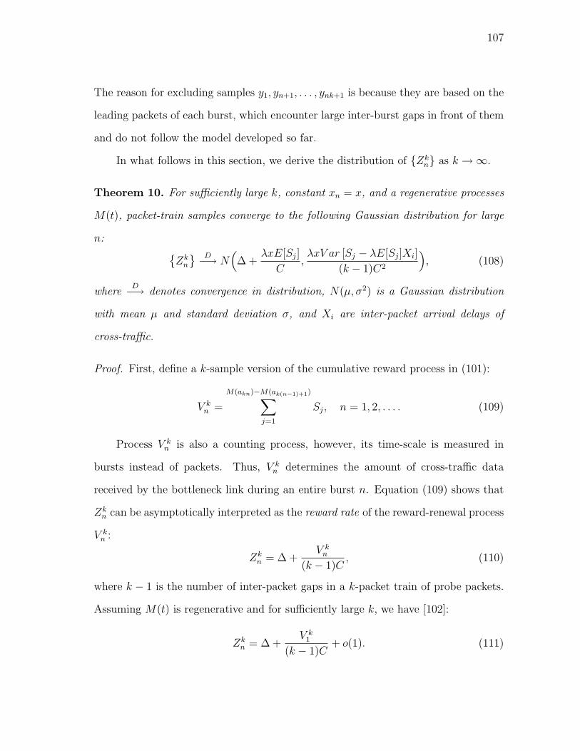
107

The reason for excluding samples y1, yn+1, . . . , ynk+1 is because they are based on the

leading packets of each burst, which encounter large inter-burst gaps in front of them

and do not follow the model developed so far.

In what follows in this section, we derive the distribution of {Zkn} as k →∞.

Theorem 10. For sufficiently large k, constant xn = x, and a regenerative processes

M(t), packet-train samples converge to the following Gaussian distribution for large

n:{Zk

n

} D−→ N(∆ +

λxE[Sj]

C,λxV ar [Sj − λE[Sj]Xi]

(k − 1)C2

), (108)

whereD−→ denotes convergence in distribution, N(µ, σ2) is a Gaussian distribution

with mean µ and standard deviation σ, and Xi are inter-packet arrival delays of

cross-traffic.

Proof. First, define a k-sample version of the cumulative reward process in (101):

V kn =

M(akn)−M(ak(n−1)+1)∑j=1

Sj, n = 1, 2, . . . . (109)

Process V kn is also a counting process, however, its time-scale is measured in

bursts instead of packets. Thus, V kn determines the amount of cross-traffic data

received by the bottleneck link during an entire burst n. Equation (109) shows that

Zkn can be asymptotically interpreted as the reward rate of the reward-renewal process

V kn :

Zkn = ∆ +

V kn

(k − 1)C, (110)

where k − 1 is the number of inter-packet gaps in a k-packet train of probe packets.

Assuming M(t) is regenerative and for sufficiently large k, we have [102]:

Zkn = ∆ +

V k1

(k − 1)C+ o(1). (111)

108

Applying the regenerative central limit theorem, constraining the rest of the

derivations in this section to constant xn = x, and assuming E[Xi] < ∞ [102]:

{V k

1

k − 1

}D−→ N

(λxE[Sj],

λxV ar [Sj − λE[Sj]Xi]

k − 1

). (112)

Combining (111) and (112), we get (108).

First, notice that the mean of this distribution is the same as that of samples {yn}in (107), which, as was intuitively expected, means that both measurement methods

have the same expectation. Second, it is also easy to notice that the variance of Zkn

tends to zero as long as V ar[Xi] is finite.

Theorem 11. If V ar[Xi] is finite, the variance of packet-train samples Zkn tends to

zero for large k.

Proof. Since λ, x, and E[Sj] are all finite and do not depend on k, using independence

of Sj and Xi in (108), we have:

V ar[Zkn] =

λxV ar[Sj] + λ3xE2[Sj]V ar[Xi]

(k − 1)C2, (113)

which tends to 0 for k →∞.

As a result of this phenomenon, longer packet trains will produce narrower dis-

tributions centered at ∆+E[ωn]. The CBR case already studied in Fig. 29(b) clearly

has finite V ar[Xi] and therefore samples {Zkn} must exhibit decaying variance as k

increases. One example of this convergence for packet trains with k = 5 and k = 10

is shown in Fig. 32.

4. Discussion

Now we address several observations of previous work. It is noted in [22] that while

packet-pair histograms usually have many different modes, the histogram of packet-

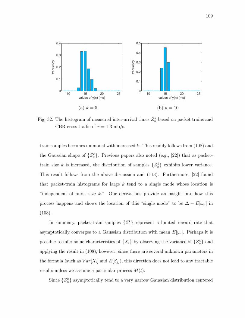
109

10 15 20 250

0.1

0.2

0.3

0.4

values of y(n) (ms)

fre

qu

en

cy

(a) k = 5

10 15 20 250

0.1

0.2

0.3

0.4

0.5

values of y(n) (ms)

fre

qu

en

cy

(b) k = 10

Fig. 32. The histogram of measured inter-arrival times Zkn based on packet trains and

CBR cross-traffic of r = 1.3 mb/s.

train samples becomes unimodal with increased k. This readily follows from (108) and

the Gaussian shape of {Zkn}. Previous papers also noted (e.g., [22]) that as packet-

train size k is increased, the distribution of samples {Zkn} exhibits lower variance.

This result follows from the above discussion and (113). Furthermore, [22] found

that packet-train histograms for large k tend to a single mode whose location is

“independent of burst size k.” Our derivations provide an insight into how this

process happens and shows the location of this “single mode” to be ∆ + E[ωn] in

(108).

In summary, packet-train samples {Zkn} represent a limited reward rate that

asymptotically converges to a Gaussian distribution with mean E[yn]. Perhaps it is

possible to infer some characteristics of {Xi} by observing the variance of {Zkn} and

applying the result in (108); however, since there are several unknown parameters in

the formula (such as V ar[Xi] and E[Sj]), this direction does not lead to any tractable

results unless we assume a particular process M(t).

Since {Zkn} asymptotically tend to a very narrow Gaussian distribution centered

110

at ∆ + E[ωn], we find that there is no evidence that {Zkn} measure the available

bandwidth or offer any additional information about the value of ∆ as compared to

traditional packet-pair samples {yn}.

D. Arbitrary Cross-Traffic

In this section, we relax the stationarity and renewal assumptions about cross-traffic

and derive a robust estimator of C and r. Assume an arbitrary arrival process r(t)

for cross-traffic, where r(t) is its instantaneous rate at time t. We impose only one

constraint on this process – it must have a finite time average r shown in (97). The

goal of the sampling process is to determine both C and r. Since r > C imply constant

packet loss and zero available bandwidth, we are generally interested in non-trivial

cases of r ≤ C. Stochastic process r(t) may be renewal, regenerative, a superposition

of ON/OFF sources, self-similar, or otherwise. Furthermore, since packet arrival

patterns in the current Internet commonly exhibit non-stationarity (due to day-night

cycles, routing changes, link failure, etc.), our assumptions on r(t) allow us to model

a wide variety of such non-stationary processes and are much broader than commonly

assumed in traffic modeling literature.

Next, notice that if the probing traffic can sample r(t) using a Poisson sequence

of probes at times t1, t2, . . ., the average of r(ti) converges to r (applying the PASTA

principle [102]):

limn→∞

r(t1) + r(t2) + ... + r(tn)

n= lim

t→∞1

t

t∫

0

r(u)du = r, (114)

as long as delays τi = ti − ti−1 are i.i.d. exponential random variables. In order to

accomplish this type of sampling, the sender must emit packet-pairs at exponentially

distributed intervals. Assuming that the i-th packet-pair arrives to the router at time

111

ti, it will sample a small segment of r(t) by allowing gi amount of data to be queued

between the probes:

gi =

ti+xi∫

ti

r(u)du ≈ r(ti)xi, (115)

where xi is the spacing between the packets in the i-th packet-pair. Again, assuming

that yi is the i-th inter-arrival sample generated by the receiver, we have:

yi = ∆ +gi

C= ∆ +

r(ti)xi

C. (116)

Finally, fixing the value of xi = x, notice that Wn has a well-defined limit:

limn→∞

Wn = limn→∞

1

n

n∑i=1

(∆ +

r(ti)xi

C

)= ∆ +

x

Clim

n→∞

n∑i=1

r(ti)

n= ∆ +

xr

C. (117)

In essence, this result4 is similar to our earlier derivations, except that (117)

requires much weaker restrictions on cross-traffic and also shows that a single-node

model is completely tractable in the setting of almost arbitrary cross-traffic. We next

show how to extract both C and r from (117).

1. Capacity

Observe that (117) is a linear function of x, where r is the slope and ∆ is the intercept5.

Therefore, by injecting packet-pairs with two different spacings xa and xb, one can

compute the unknown terms in (117) using two sets of measurements {yai } and {yb

i}.To accomplish this, define the corresponding average processes to be W a

n and W bn:

W an =

1

n

n∑i=1

yai , W b

n =1

n

n∑i=1

ybi . (118)

4A similar formula has been derived in [10], [37], [72] and several other papersunder a fluid assumption.

5For technical differences between this approach and previous work (such as TOPP[72]), see [60].

112

The simplest way to obtain both W an and W b

n using a single measurement is to

alternate spacing xa and xb while preserving the PASTA sampling property. Using a

one-bit header field, the receiver can unambiguously sort the inter-arrival delays into

two sets {yai } and {yb

i}, and thus compute their averages in (118).

While samples are being collected, the receiver has two running averages pro-

duced by (118). Subtracting W bn from W a

n , we are able to separate r/C from ∆:

limn→∞

(W an −W b

n) =(xa − xb)r

C. (119)

Next, denote by ∆n the following estimate of ∆ at time n:

∆n = W an − xa

W an −W b

n

xa − xb

. (120)

Taking the limit of (120), we have the following result.

Theorem 12. Assuming a single congested bottleneck for which time-average rate r

exists, ∆n converges to ∆:

limn→∞

∆n = ∆. (121)

Proof. Re-writing (121):

limn→∞

∆n = ∆ +xar

C− xa

(xa − xb)r

C(xa − xb)= ∆, (122)

which is obtained with the help of (117), (119), and (120).

Our next result shows a more friendly restatement of the previous claim.

Corollary 13. Assuming a single congested bottleneck for which time-average rate r

exists, estimate Cn = q/∆n converges to capacity C:

limn→∞

Cn = limn→∞

q

W an − xa

W an −W b

n

xa − xb

= limn→∞

q(xa − xb)

xaW bn − xbW a

n

= C. (123)

113

2. Available Bandwidth

Notice that knowing an estimate of C in (123) and using r in (119), it is easy to

estimate the mean rate of cross-traffic:

limn→∞

(W an −W b

n)Cn

xa − xb

= r, (124)

which leads to the following result.

Corollary 14. Assuming a single congested bottleneck for which time-average rate r

exists, the following converges to the available bandwidth A = C − r:

limn→∞

q

(xa − xb −W a

n + W bn

xaW bn − xbW a

n

)= C − r = A. (125)

3. Simulations

We confirm these results and compare our models with several recent methods Spruce

[96], IGI [37], and Pathload [44] through ns2 simulations. Since the main theme of

this chapter is bandwidth estimation in heavily-congested routers, we conduct all

simulations over a loaded bottleneck link in Fig. 28 with utilization varying between

82% and 92% (the exact value changes depending on C and the interaction of TCP

cross-traffic with probe packets). Delays xa and xb are set to maintain the desired

range of link utilization.

Define eA = |A−A|/A and eC = |C − C|/C to be the relative estimation errors

of A and C, respectively, where A is the true available bandwidth of a path, A is its

estimate using one of the measurement techniques, C is the true bottleneck capacity,

and C is its estimate. Table X shows relative estimation errors eA for Pathload,

Spruce, and IGI. For Pathload, we averaged the low and high values of the produced

estimates A. In the IGI case, we used the estimates available at the end of IGI’s

internal convergence algorithm. Also note that we fed both Spruce and IGI the

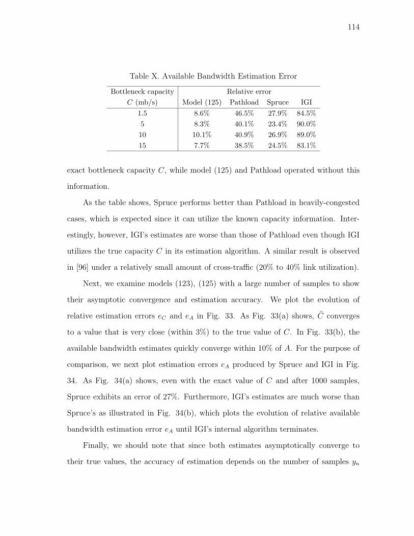
114

Table X. Available Bandwidth Estimation Error

Bottleneck capacity Relative errorC (mb/s) Model (125) Pathload Spruce IGI

1.5 8.6% 46.5% 27.9% 84.5%5 8.3% 40.1% 23.4% 90.0%10 10.1% 40.9% 26.9% 89.0%15 7.7% 38.5% 24.5% 83.1%

exact bottleneck capacity C, while model (125) and Pathload operated without this

information.

As the table shows, Spruce performs better than Pathload in heavily-congested

cases, which is expected since it can utilize the known capacity information. Inter-

estingly, however, IGI’s estimates are worse than those of Pathload even though IGI

utilizes the true capacity C in its estimation algorithm. A similar result is observed

in [96] under a relatively small amount of cross-traffic (20% to 40% link utilization).

Next, we examine models (123), (125) with a large number of samples to show

their asymptotic convergence and estimation accuracy. We plot the evolution of

relative estimation errors eC and eA in Fig. 33. As Fig. 33(a) shows, C converges

to a value that is very close (within 3%) to the true value of C. In Fig. 33(b), the

available bandwidth estimates quickly converge within 10% of A. For the purpose of

comparison, we next plot estimation errors eA produced by Spruce and IGI in Fig.

34. As Fig. 34(a) shows, even with the exact value of C and after 1000 samples,

Spruce exhibits an error of 27%. Furthermore, IGI’s estimates are much worse than

Spruce’s as illustrated in Fig. 34(b), which plots the evolution of relative available

bandwidth estimation error eA until IGI’s internal algorithm terminates.

Finally, we should note that since both estimates asymptotically converge to

their true values, the accuracy of estimation depends on the number of samples yn

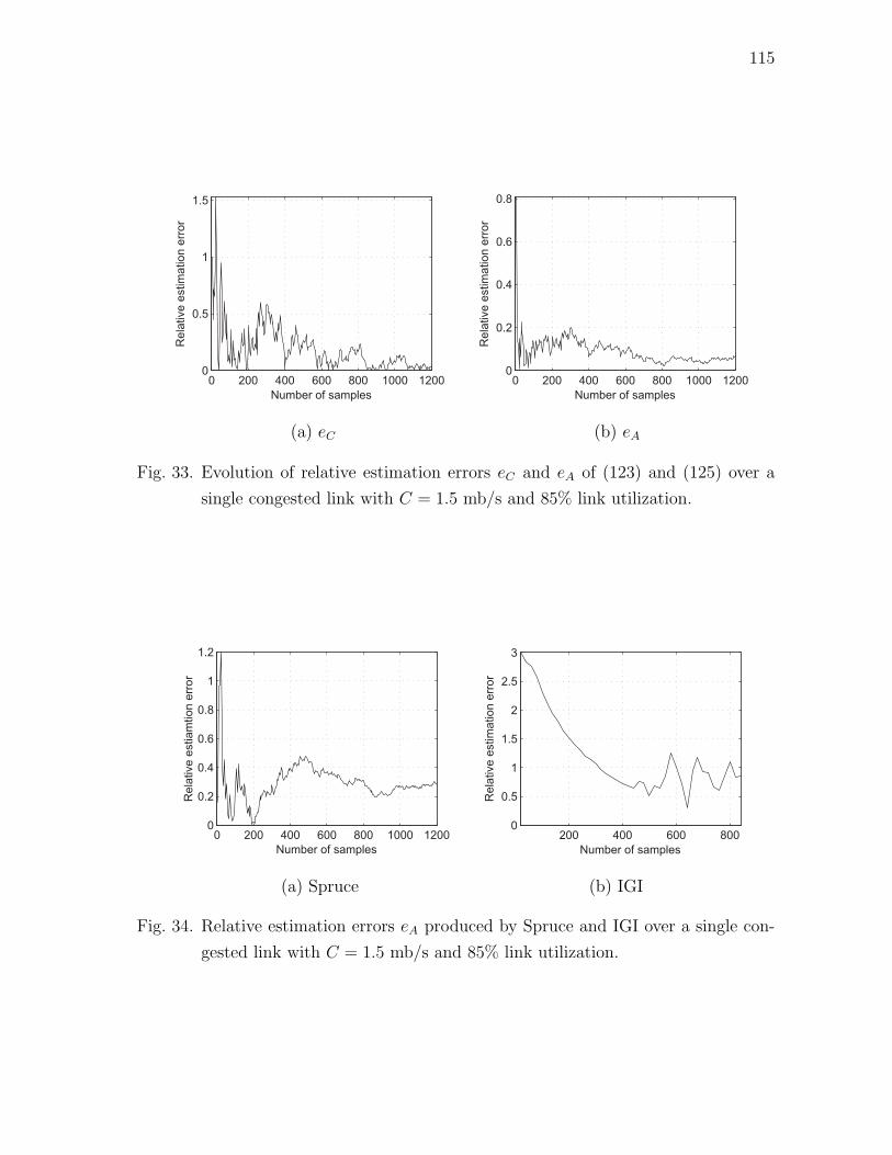
115

0 200 400 600 800 1000 12000

0.5

1

1.5

Number of samples

Re

lative

estim

atio

n e

rro

r

(a) eC

0 200 400 600 800 1000 12000

0.2

0.4

0.6

0.8

Number of samples

Re

lative

estim

atio

n e

rro

r

(b) eA

Fig. 33. Evolution of relative estimation errors eC and eA of (123) and (125) over a

single congested link with C = 1.5 mb/s and 85% link utilization.

0 200 400 600 800 1000 12000

0.2

0.4

0.6

0.8

1

1.2

Number of samples

Rela

tive e

stiam

tion e

rror

(a) Spruce

200 400 600 8000

0.5

1

1.5

2

2.5

3

Number of samples

Re

lative

estim

atio

n e

rro

r

(b) IGI

Fig. 34. Relative estimation errors eA produced by Spruce and IGI over a single con-

gested link with C = 1.5 mb/s and 85% link utilization.

116

used. This provides operational flexibility to applications because there exists trade-

off between accuracy and time for measurements.

E. Extension to Multiple Links

In this section, we discuss possibility of extension of our single-node model to the case

of multiple congested routers and conjecture that such extension may be possible pro-

vided that a certain queuing condition of probe packets holds. We start by discussing

in the next subsection the case that the probe packets do not queue behind each other

at the bottleneck router, which may occur on a path with multiple congested routers.

1. Large Inter-Probe Delays

Consider the original model of a router in (98). This time, assume that none of the

probe packets queue behind each other at the bottleneck router. This means that

packet n−1 leaves the router before packet n arrives, which is expected if inter-packet

spacing xn at the source is very large compared to the transmission delay ∆. Under

these assumptions, dn−1 < an and (98) becomes:

dn = an + ωn + ∆, n ≥ 1. (126)

Hence, inter-departure delays yn are:

yn = an − an−1 + ωn − ωn−1, n ≥ 2. (127)

Notice that the first term an − an−1 in (127) is the inter-arrival delay xn of the

probe traffic and the second term ωn−ωn−1 can be modeled as some zero-mean random

noise. This can be explained intuitively by noticing that under the assumption of large

xn, each router delays probe packets (on average) by the same amount. Then the

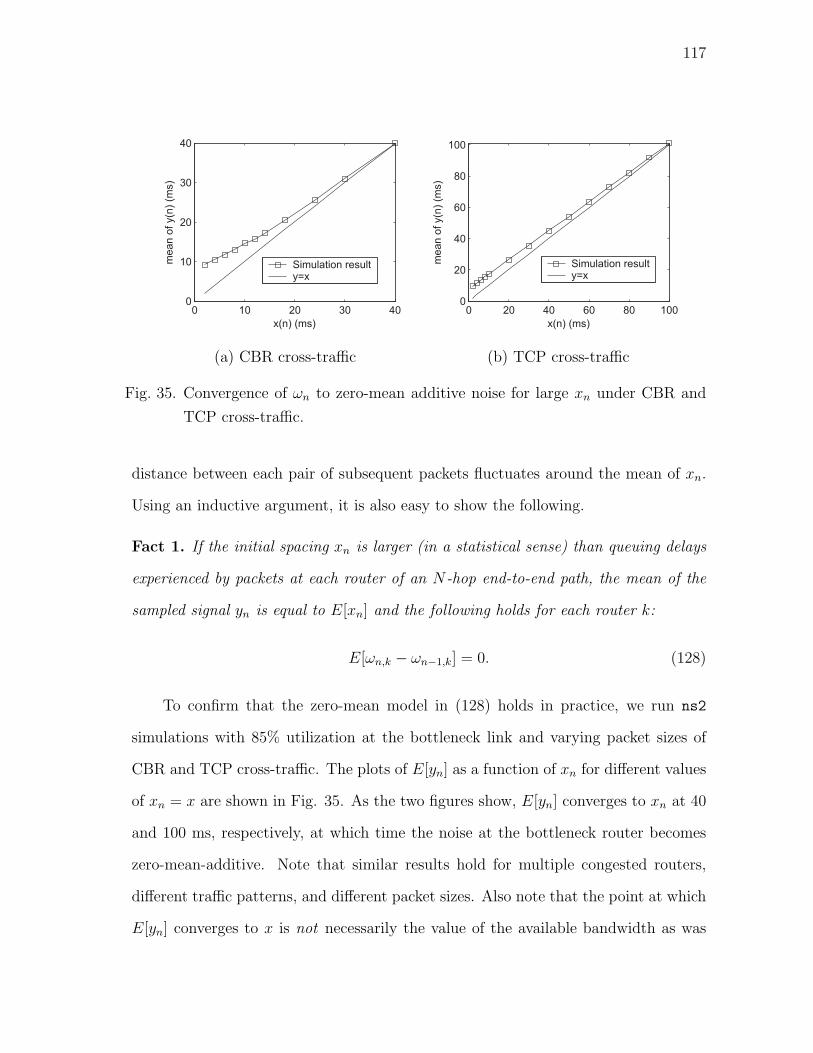
117

0 10 20 30 400

10

20

30

40

x(n) (ms)

mean o

f y(n

) (m

s)

Simulation resulty=x

(a) CBR cross-traffic

0 20 40 60 80 1000

20

40

60

80

100

x(n) (ms)

mean o

f y(n

) (m

s)

Simulation resulty=x

(b) TCP cross-traffic

Fig. 35. Convergence of ωn to zero-mean additive noise for large xn under CBR and

TCP cross-traffic.

distance between each pair of subsequent packets fluctuates around the mean of xn.

Using an inductive argument, it is also easy to show the following.

Fact 1. If the initial spacing xn is larger (in a statistical sense) than queuing delays

experienced by packets at each router of an N-hop end-to-end path, the mean of the

sampled signal yn is equal to E[xn] and the following holds for each router k:

E[ωn,k − ωn−1,k] = 0. (128)

To confirm that the zero-mean model in (128) holds in practice, we run ns2

simulations with 85% utilization at the bottleneck link and varying packet sizes of

CBR and TCP cross-traffic. The plots of E[yn] as a function of xn for different values

of xn = x are shown in Fig. 35. As the two figures show, E[yn] converges to xn at 40

and 100 ms, respectively, at which time the noise at the bottleneck router becomes

zero-mean-additive. Note that similar results hold for multiple congested routers,

different traffic patterns, and different packet sizes. Also note that the point at which

E[yn] converges to x is not necessarily the value of the available bandwidth as was

118

suggested in prior work [37].

2. Recursive Model for Multi-Node Paths

Assuming multiple congested routers along a path, the result in (121) no longer holds.

Notice that it is possible to recursively extend the original model in (117) to multiple

congested links where the input xn of each link is the output yn of the previous link.

Add index k to each process and each random variable to indicate that it is local

to router k along the path from the sender to the receiver. Define xi,k to be the inter-

packet spacing of two probe packets P2i and P2i−1 in a probe-pair i arriving at router

Rk and yi,k to be their inter-departure spacing exiting from Rk. Denote by ω2i,k the

random noise introduced to the spacing between P2i and P2i−1 by the cross-traffic at

Rk. Further denote by Q2i−1,k the queuing delay of the first probe packet P2i−1 in the

i-th probe-pair inside router Rk and φ2i,k is some zero-mean noise process of the i-th

pair at Rk. Then, we define the following recursive model:

yi,k =

∆k + ω2i,k, xi,k < Q2i−1,k

∆k + φ2i,k, xi,k ≥ Q2i−1,k

, (129)

where ∆k = q/Ck is the transmission delay of the probe packets over link k (where

Ck is the capacity of router Rk).

Notice that inter-arrival spacing xi,k of probe traffic at router Rk simply equals

inter-departure delay yi,k−1 of the previous router Rk−1. Further notice that if inter-

arrival spacing xi,k between two packets in a probe-pair i is less than the time that the

second probe packet in the pair spends in the buffer, the two packets queue behind

each other and follow the model developed earlier in this chapter. When the opposite

holds, the packets do not queue behind each other and the router adds i.i.d. zero-mean

noise φ2i,k to ∆k.

119

F. Measuring Tight-Link Bandwidth over Multi-Hop Paths

Although it appears impossible to completely tract the multi-hop paths due to the

stochastic mixture of two types of noise in (129), a recent probing method (called

Envelop) aims to measure end-to-end multi-hop paths by achieving the two conditions

in (129). This sampling technique sends trains of N probe packets surrounded by

two envelope packets along the path in question and allows the probe packets to

sample queuing dynamics at the desired router Rk and then “disappear” from the

network at router Rk+1. If the length of a packet-train is sufficiently large, then the

recursive relationship between the average output dispersions E[yi,k] and E[yi,k−1] can

be expressed as:

E[yi,k] =

E[yi,k−1] E[yi,k−1] ≥ q

Ak

q + λkE[yi,k−1]

Ck

E[yi,k−1] <q

Ak

, (130)

where Ck and Ak are the respective capacity and available bandwidth of router Rk, q

is the size of probing packets, and λk is the average arrival rate of cross-traffic entering

Rk.

It is easy to see from (130) that a necessary condition for the bandwidth char-

acteristics of link Rk to be measurable is E[yi,k−1] < q/Ak. Otherwise, Rk preserves

average incoming inter-packet spacings and thus E[yi,k] contains no information about

the capacity or available bandwidth of the link. Define Rt to be the tight-link router

and At to be the tight-link available bandwidth. Then, the above conditions can be

summarized as following.

Fact 2. The tight-link router Rt is always measurable as long as the initial spacing

x < q/At.

Fact 3. The mean inter-departure delay E[yi,k] of router Rk is preserved along the

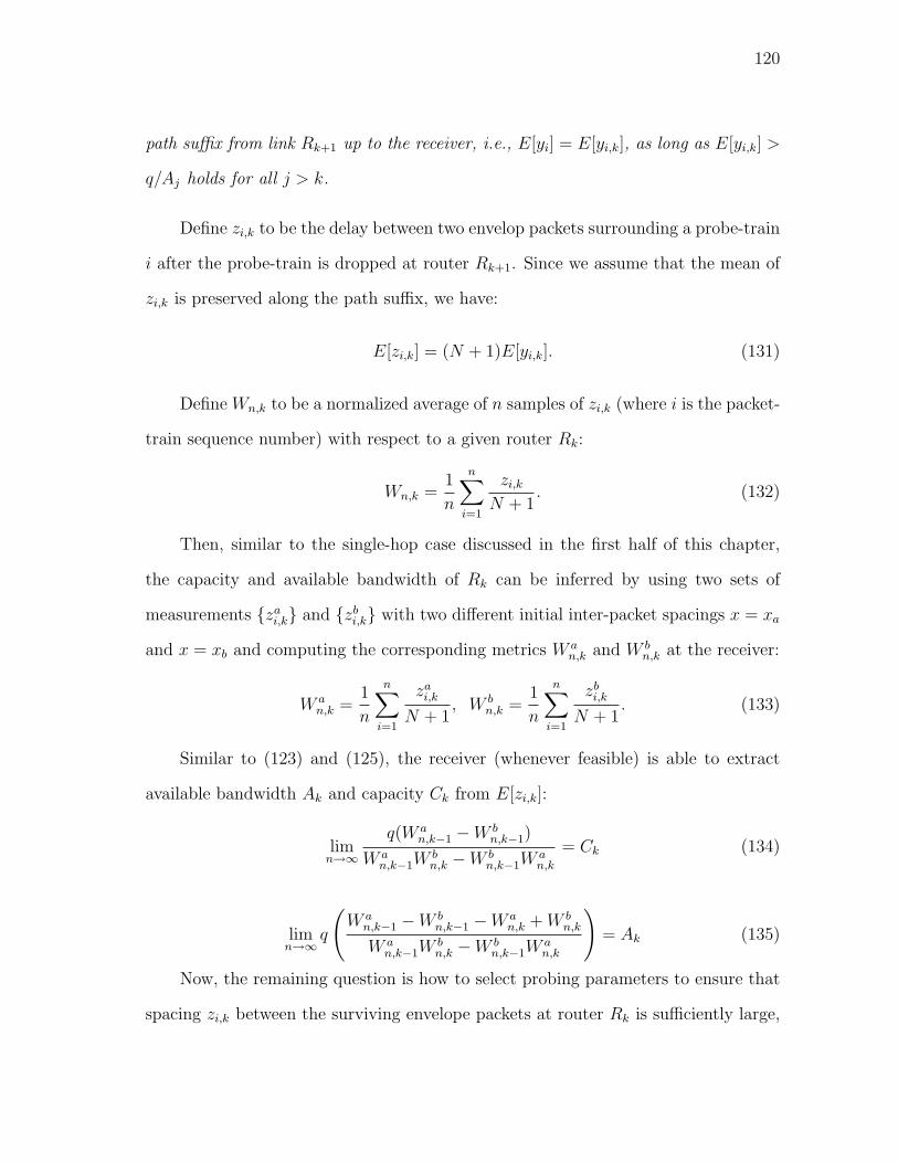
120

path suffix from link Rk+1 up to the receiver, i.e., E[yi] = E[yi,k], as long as E[yi,k] >

q/Aj holds for all j > k.

Define zi,k to be the delay between two envelop packets surrounding a probe-train

i after the probe-train is dropped at router Rk+1. Since we assume that the mean of

zi,k is preserved along the path suffix, we have:

E[zi,k] = (N + 1)E[yi,k]. (131)

Define Wn,k to be a normalized average of n samples of zi,k (where i is the packet-

train sequence number) with respect to a given router Rk:

Wn,k =1

n

n∑i=1

zi,k

N + 1. (132)

Then, similar to the single-hop case discussed in the first half of this chapter,

the capacity and available bandwidth of Rk can be inferred by using two sets of

measurements {zai,k} and {zb

i,k} with two different initial inter-packet spacings x = xa

and x = xb and computing the corresponding metrics W an,k and W b

n,k at the receiver:

W an,k =

1

n

n∑i=1

zai,k

N + 1, W b

n,k =1

n

n∑i=1

zbi,k

N + 1. (133)

Similar to (123) and (125), the receiver (whenever feasible) is able to extract

available bandwidth Ak and capacity Ck from E[zi,k]:

limn→∞

q(W an,k−1 −W b

n,k−1)

W an,k−1W

bn,k −W b

n,k−1Wan,k

= Ck (134)

limn→∞

q

(W a

n,k−1 −W bn,k−1 −W a

n,k + W bn,k

W an,k−1W

bn,k −W b

n,k−1Wan,k

)= Ak (135)

Now, the remaining question is how to select probing parameters to ensure that

spacing zi,k between the surviving envelope packets at router Rk is sufficiently large,

121

while minimizing probing overhead as much as possible and maximizing the number

of links measurable. We address this by developing a measurement tool by adaptively

selecting various probing parameters based on different path conditions.

1. Probing Parameters in Envelope

The main idea behind Envelope is to preserve the inter-departure spacing yi,k of

probe packets in the path suffix of a congested router Rk using envelope packets.

As suggested in Section E, maintaining a large inter-envelope packet spacing zi,k

preserves its mean E[zi,k] in the path suffix since cross-traffic noise introduced into

zi,k becomes zero-mean. Note that spacing zi,k depends on the capacity of routers

Rj (j ≤ k), amount of cross-traffic interfering with probe packets at Rj, initial input

spacing x, and probe-train length N . Since only x and N can be controlled by the

Envelope source, proper selection of N and x is important in producing sufficiently

large zi,k (manual selection of such parameters which is done by the previous work

cannot determine optimal values of N and x under dynamically changing network

conditions).

Hence, in the following subsections, we investigate a method that automatically

selects these parameters in practice such that E[zi,k] is preserved through the path

suffix after the tight link. We start by discussing two initial input spacings x = xa

and x = xb and how Envelope chooses them.

a. Initial Input Spacing

Recall from Fact 2 that as long as the two spacings are less than q/At and differ from

each other, the tight link can be measured. Note that Envelope can also measure

many non-tight links if the conditions in Facts 2 and 3 hold. Hence, it makes sense

to choose at least one initial spacing that is much smaller than q/At. To achieve

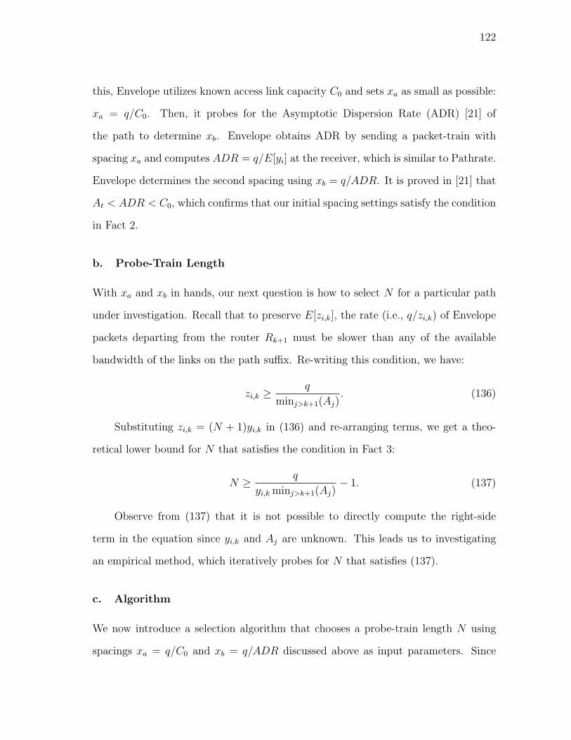
122

this, Envelope utilizes known access link capacity C0 and sets xa as small as possible:

xa = q/C0. Then, it probes for the Asymptotic Dispersion Rate (ADR) [21] of

the path to determine xb. Envelope obtains ADR by sending a packet-train with

spacing xa and computes ADR = q/E[yi] at the receiver, which is similar to Pathrate.

Envelope determines the second spacing using xb = q/ADR. It is proved in [21] that

At < ADR < C0, which confirms that our initial spacing settings satisfy the condition

in Fact 2.

b. Probe-Train Length

With xa and xb in hands, our next question is how to select N for a particular path

under investigation. Recall that to preserve E[zi,k], the rate (i.e., q/zi,k) of Envelope

packets departing from the router Rk+1 must be slower than any of the available

bandwidth of the links on the path suffix. Re-writing this condition, we have:

zi,k ≥ q

minj>k+1(Aj). (136)

Substituting zi,k = (N + 1)yi,k in (136) and re-arranging terms, we get a theo-

retical lower bound for N that satisfies the condition in Fact 3:

N ≥ q

yi,k minj>k+1(Aj)− 1. (137)

Observe from (137) that it is not possible to directly compute the right-side

term in the equation since yi,k and Aj are unknown. This leads us to investigating

an empirical method, which iteratively probes for N that satisfies (137).

c. Algorithm

We now introduce a selection algorithm that chooses a probe-train length N using

spacings xa = q/C0 and xb = q/ADR discussed above as input parameters. Since

123

……

Fig. 36. A probe-train of m packets that is used for parameter tuning.

Envelope requires xa 6= xb, it chooses two values Na and Nb for the train length N in

order to sample cross-traffic statistics with two different time spans xaNa and xbNb

at routers along the path. Intuitively, cross-traffic arriving over a time interval xaN

or xbN is more bursty for smaller N . Hence, we can sample cross-traffic statistics

more accurately with larger time spans (using large Na and Nb). However, since

measurement overhead also increases with N , it is preferable to keep N as small

as possible. Based on the above discussion and the trade-off between accuracy and

overhead, we develop an automated algorithm that selects N = Na and N = Nb, each

of which is large enough to preserve the mean of inter-envelope packet spacings, while

minimizing measurement overhead under various network path conditions.

Define Nl and Nh to be a minimum and maximum train lengths, respectively.

Further define σ to be a certain threshold that is adjustable between zero and one.

Our parameter tuning procedure (Algorithm 1) includes two subroutines called adjust-

spacing (Algorithm 2) and binary-tuning (Algorithm 3), where the former searches

for the smallest value of xa that satisfies the mean preservation condition for the

given maximum train length Nh and the latter optimizes the train length N for

selected initial input spacings xa and xb. Both sub-procedures include an additional

subroutine called probe-run (Algorithm 4), which tests if a particular input spacing

z = xN is preserved in the path by sending to the receiver a train of m probe packets

P1, P2, . . . , Pm (1500 bytes each) with inter-packet spacing z as shown in Fig. 36.

124

Algorithm 1 Parameter tuning

1: xa ← q/C0, xb ← q/ADR2: xa ← adjust-spacing(xa, Nh)3: Na ← binary-tuning(Nl, Nh, xa)4: Nb ← binary-tuning(Nl, Na, xb)

Algorithm 2 adjust-spacing(x,N)

1: while probe-run(x,N) = true do2: x ← 2x3: if x ≥ xb/β then4: notify to the user that N = Nh is too small and stop5: end if6: end while7: return x

To assess the preservation of input spacing z, the probe-run procedure computes the

following relative error metric ez:

ez =|z − z|

z, (138)

where z represents an m-sample average of output inter-packet spacings sampled at

the receiver. When ez > σ, the routine returns true; otherwise, it returns false.

Note that if more than the half of probe packets in a probe-train are lost, then the

receiver discards that probe train (this implementation details are not shown in the

algorithms).

The parameter selection procedure (Algorithm 1) operates as follows. If input

spacing z = qNh/C0 is not preserved in the path, Envelope keeps doubling xa until the

input spacing is preserved or xa reaches a certain fraction of q/ADR (step 2). When

Envelope finds xa that satisfies the preservation for N = Nh, it probes for an optimal

value of Na with current xa using a binary search (step 3). Thereafter, Envelope

repeats the binary search in step 4 to determine an optimal value for Nb. Note that

in step 2, the probe-run subroutine is repeatedly used for parameter optimization and

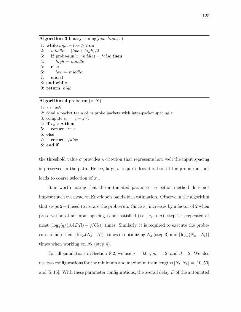
125

Algorithm 3 binary-tuning(low, high, x)

1: while high− low ≥ 2 do2: middle ← (low + high)/23: if probe-run(x, middle) = false then4: high ← middle5: else6: low ← middle7: end if8: end while9: return high

Algorithm 4 probe-run(x,N)

1: z ← xN2: Send a packet train of m probe packets with inter-packet spacing z3: compute ez = |z − z|/z4: if ez > σ then5: return true6: else7: return false8: end if

the threshold value σ provides a criterion that represents how well the input spacing

is preserved in the path. Hence, large σ requires less iteration of the probe-run, but

leads to coarse selection of xa.

It is worth noting that the automated parameter selection method does not

impose much overhead on Envelope’s bandwidth estimation. Observe in the algorithm

that steps 2−4 need to iterate the probe-run. Since xa increases by a factor of 2 when

preservation of an input spacing is not satisfied (i.e., ez > σ), step 2 is repeated at

most blog2(q/(βADR)− q/C0)c times. Similarly, it is required to execute the probe-

run no more than blog2(Nh−Nl)c times in optimizing Na (step 3) and blog2(Na−Nl)ctimes when working on Nb (step 4).

For all simulations in Section F.2, we use σ = 0.05, m = 12, and β = 2. We also

use two configurations for the minimum and maximum train lengths [Nl, Nh] = [10, 50]

and [5, 15]. With these parameter configurations, the overall delay D of the automated

126

R1 R2 R3C1

C2R4 R5

C3

C4

PR

PS

S1 D1 S3 D3

S2 D2 S4 D4

100 Mb/s

5 ms

100 Mb/s

5 ms

100 Mb/s

5 ms

100 Mb/s

5 ms

100 Mb/s

5 ms

100 Mb/s

5 ms

100 Mb/s

5 ms

100 Mb/s

5 ms

100 Mb/s

5 ms

100 Mb/s

5 ms

Fig. 37. Simulation topology.

parameter tuning is no more than 5 seconds under various network conditions studied

in this chapter (see Tables XI – XIV for details). Note that the parameter selection

procedure can accept values for the minimum and maximum train lengths Nl and Nh

as an input, which allows users to decide the tradeoff between measurement overhead

and estimation accuracy.

2. Performance of Envelope

To evaluate the performance of Envelope, we use simulations to measure estimation

accuracy and asymptotic behavior and then compare these results with those in ex-

isting methods. We start by describing the simulation setup.

a. Simulation Setup

For simulations, we use the ns2 network simulator [73] with the topology shown in

Fig. 37, in which source PS sends probe data to the destination PR through five router

nodes R1, . . . , R5. Cross-traffic is injected into each router Ri (where i = 1, 2, 3, 4) at

an average rate λi through nodes Si (i = 1, 2, 3, 4). The speed of all access links is

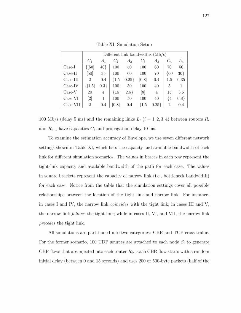
127

Table XI. Simulation Setup

Different link bandwidths (Mb/s)C1 A1 C2 A2 C3 A3 C4 A4

Case-I {[50] 40} 100 50 100 60 70 50Case-II [50] 35 100 60 100 70 {60 30}Case-III 2 0.4 {1.5 0.25} [0.8] 0.4 1.5 0.35Case-IV {[1.5] 0.3} 100 50 100 40 5 1Case-V 20 4 {15 2.5} [8] 4 15 3.5Case-VI [2] 1 100 50 100 40 {4 0.8}Case-VII 2 0.4 [0.8] 0.4 {1.5 0.25} 2 0.4

100 Mb/s (delay 5 ms) and the remaining links Li (i = 1, 2, 3, 4) between routers Ri

and Ri+1 have capacities Ci and propagation delay 10 ms.

To examine the estimation accuracy of Envelope, we use seven different network

settings shown in Table XI, which lists the capacity and available bandwidth of each

link for different simulation scenarios. The values in braces in each row represent the

tight-link capacity and available bandwidth of the path for each case. The values

in square brackets represent the capacity of narrow link (i.e., bottleneck bandwidth)

for each case. Notice from the table that the simulation settings cover all possible

relationships between the location of the tight link and narrow link. For instance,

in cases I and IV, the narrow link coincides with the tight link; in cases III and V,

the narrow link follows the tight link; while in cases II, VI, and VII, the narrow link

precedes the tight link.

All simulations are partitioned into two categories: CBR and TCP cross-traffic.

For the former scenario, 100 UDP sources are attached to each node Si to generate

CBR flows that are injected into each router Ri. Each CBR flow starts with a random

initial delay (between 0 and 15 seconds) and uses 200 or 500-byte packets (half of the

128

CBR flows uses 200-byte packets, while the other half employs 500-byte packets)6.

For simulations with TCP cross-traffic, we attach 100 FTP sources to each of Si and

keep the utilization of each router Ri according to the values shown in Table XI. To

maintain a fixed average utilization at each link in the TCP scenario, we place an

additional router (not shown in the figure) between each node Si and router Ri to

limit the aggregate sending rate of the TCP flows to the capacity of the additional

router. The utilization of Ri is controlled by properly setting the capacity of the

auxiliary router. TCP cross-traffic consists of a mixture of flows with packet sizes

40, 572, and 1500 bytes, which are selected according to several measurement studies

[30], [99] that demonstrate that Internet packet sizes exhibit a trimodal distribution.

In both TCP and UDP scenarios, link utilization along the path of probe pack-

ets varies between 20% and 50% for cases I and II (mild-load traffic scenarios) and

between 50% and 83% for cases III – VII (heavy-load traffic scenarios).

Under this setup, the probe-traffic source PS starts at 60 seconds and sends

trains with 1500-byte packets to measure the path. We use fixed delay between

two probe trains instead of using exponentially distributed delay since the benefit of

Poisson sampling over fixed-interval sampling is marginal [4]. To avoid congesting

the network, Envelope uses low average probing rates for each path depending on

measured ADR. Specifically, Envelope sets its probing rate to 50 kb/s for a path with

ADR < 1 Mb/s, 100 kb/s with 1 < ADR ≤ 5 Mb/s, 250 kb/s for 5 < ADR ≤ 10

Mb/s, and 500 kb/s for ADR > 10 Mb/s. Lengths Na and Nb of alternate packet-

trains and inter-packet spacings xa and xb are automatically selected as discussed in

the previous section.

Note that every simulation has four phases, one for each link in Fig. 37. In each

6We remind that the aggregated cross-traffic that actually traverses each router isnot CBR, but an aggregation of CBR flows with rather bursty characteristics.

129

phase φk (k = 1, 2, 3, 4), the packet-trains enclosed by envelope-packets are dropped

at router Rk+1, while the two envelope packets are forwarded up to the receiver.

In each phase, the receiver PR computes the average spacing W an,k and W b

n,k after

receiving n = 50 packet-trains for each spacing xa and xb. The two average spacings

are then applied to (134) and (135) to produce estimates of capacity and available

bandwidth of the router under investigation.

3. Estimation Accuracy of Envelope

We next investigate estimation accuracy of Envelope, and convergence behavior. We

first define the following relative error metrics:

eCi=|Ci − Ci|

Ci

, eAi=|Ai − Ai|

Ai

, (139)

where Ci is the true capacity of a link Li, Ci is its estimate, Ai is the true available

bandwidth of Li, and Ai is its estimate. Similarly, define eC and eA to be the respective

relative estimation errors of capacity and available bandwidth of the tight link Lt of

the path:

eC =|Ct − Ct|

Ct

, eA =|At − At|

At

, (140)

where Ct is the true capacity of the tight link Lt, Ct is its estimate, At is the true

available bandwidth of Lt, and At is its estimate.

Simulation results of Envelope are summarized in Tables XII and XIII, which

show relative estimation errors eCiand eAi

under CBR and TCP cross-traffic, respec-

tively. For these results, we conduct simulations with the minimum and maximum

train lengths Nl = 10 and Nh = 50. In the tables, parameter values selected auto-

matically by Envelope are shown in rows 11− 14 and combined delays for parameter

tuning are given in rows 15. Empty cells represent links that are not measurable

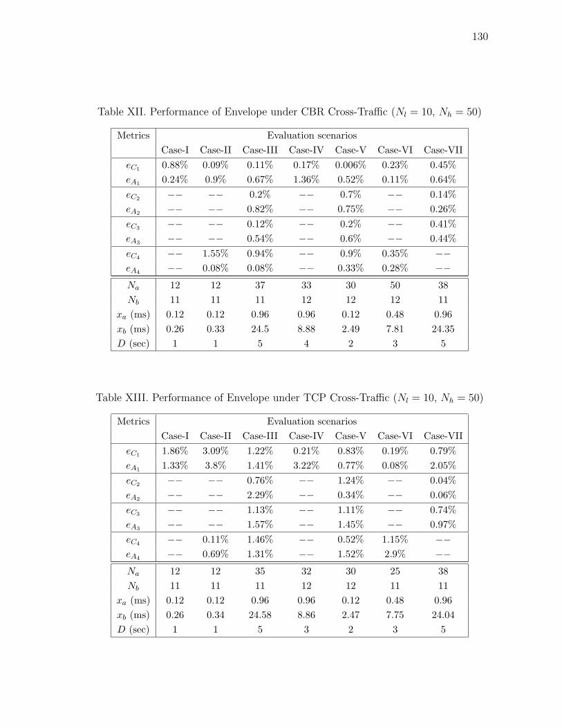
130

Table XII. Performance of Envelope under CBR Cross-Traffic (Nl = 10, Nh = 50)

Metrics Evaluation scenariosCase-I Case-II Case-III Case-IV Case-V Case-VI Case-VII

eC1 0.88% 0.09% 0.11% 0.17% 0.006% 0.23% 0.45%eA1 0.24% 0.9% 0.67% 1.36% 0.52% 0.11% 0.64%eC2 −− −− 0.2% −− 0.7% −− 0.14%eA2 −− −− 0.82% −− 0.75% −− 0.26%eC3 −− −− 0.12% −− 0.2% −− 0.41%eA3 −− −− 0.54% −− 0.6% −− 0.44%eC4 −− 1.55% 0.94% −− 0.9% 0.35% −−eA4 −− 0.08% 0.08% −− 0.33% 0.28% −−Na 12 12 37 33 30 50 38Nb 11 11 11 12 12 12 11

xa (ms) 0.12 0.12 0.96 0.96 0.12 0.48 0.96xb (ms) 0.26 0.33 24.5 8.88 2.49 7.81 24.35D (sec) 1 1 5 4 2 3 5

Table XIII. Performance of Envelope under TCP Cross-Traffic (Nl = 10, Nh = 50)



xa (ms) 0.12 0.12 0.96 0.96 0.12 0.48 0.96xb (ms) 0.26 0.34 24.58 8.86 2.47 7.75 24.04D (sec) 1 1 5 3 2 3 5

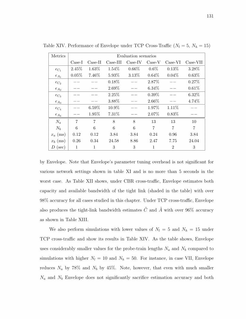
131

Table XIV. Performance of Envelope under TCP Cross-Traffic (Nl = 5, Nh = 15)



xa (ms) 0.12 0.12 3.84 3.84 0.24 0.96 3.84xb (ms) 0.26 0.34 24.58 8.86 2.47 7.75 24.04D (sec) 1 1 3 3 1 2 3

by Envelope. Note that Envelope’s parameter tuning overhead is not significant for

various network settings shown in table XI and is no more than 5 seconds in the

worst case. As Table XII shows, under CBR cross-traffic, Envelope estimates both

capacity and available bandwidth of the tight link (shaded in the table) with over

98% accuracy for all cases studied in this chapter. Under TCP cross-traffic, Envelope

also produces the tight-link bandwidth estimates C and A with over 96% accuracy

as shown in Table XIII.

We also perform simulations with lower values of Nl = 5 and Nh = 15 under

TCP cross-traffic and show its results in Table XIV. As the table shows, Envelope

uses considerably smaller values for the probe-train lengths Na and Nb compared to

simulations with higher Nl = 10 and Nh = 50. For instance, in case VII, Envelope

reduces Na by 78% and Nb by 45%. Note, however, that even with much smaller

Na and Nb Envelope does not significantly sacrifice estimation accuracy and both

132

capacity and available bandwidth of the tight link are estimated with 93% − 99%

accuracy for all studied cases.

4. Performance Comparison

In this subsection, we compare Envelope with several existing available bandwidth

estimators (Pathload [44], Spruce [96], and IGI [37]) and capacity estimation tools

(Pathrate [21] and CapProbe [49]) with respect to estimation accuracy using the

setup shown in Table XI. For Pathload, IGI, and CapProbe, we use the ns2 modules

that were obtained from the authors, while for Spruce and Pathrate, we converted

corresponding UNIX software publicly available into ns2 code.

a. Available Bandwidth Comparison

We first compare Envelope with Pathload, Spruce, and IGI. For this purpose, we

conduct all simulations under both mild-load (cases I and II) and heavy-load (cases

III – VII) traffic conditions. Note that with negligible cross-traffic interference at

non-tight links, all methods produce very accurate estimates of available bandwidth

(we do not show this result in the thesis for brevity). However, when cross-traffic

is non-negligible, the estimation accuracy is drastically different depending on the

applied methods.

Tables XV and XVI show relative estimation errors eA for the different cases

under CBR and TCP cross-traffic, respectively. For Pathload, we use up to 15600

samples with a very fine-grained bandwidth resolution of 50 kb/s and average the

low and high values of the produced estimates7. For Spruce, we obtain up to 2000

7Recall that Pathload normally exhibits better estimation accuracy with smallerbandwidth resolution, but its internal algorithm requires more samples and time toconverge.

133

Table XV. Available Bandwidth Estimation Methods (CBR Cross-Traffic)

Relative estimation error eA

Envelope Pathload Spruce IGICase-I 0.24% 1% 0.04% 0.44%Case-II 0.08% 1.66% 15.4% 19.84%Case-III 0.82% 1.4% 65.07% 62.31%Case-IV 1.36% 2.52% 1.63% 53.73%Case-V 0.75% 3.12% 67.51% 68.04%Case-VI 0.28% 1.12% 22.66% 44.24%Case-VII 0.44% 1.28% 67.84% 72.07%

Table XVI. Available Bandwidth Estimation Methods (TCP Cross-Traffic)

Relative estimation error eA

Envelope Pathload Spruce IGICase-I 1.33% 1.25% 2.47% 13.7%Case-II 0.69% 2.56% 14.5% 4.09%Case-III 2.29% 11.31% 68.07% 61.7%Case-IV 3.22% 2.53% 27.56% 237%Case-V 0.34% 6.64% 71.17% 74.28%Case-VI 2.9% 1.12% 9.9% 47.25%Case-VII 0.97% 17.98% 82.82% 55.23%

packet-pair samples (over 1200 seconds of simulation time) and then use the last 100

sample average to obtain the main estimate as suggested in [96]. In the IGI case,

we use the estimates available at the end of IGI’s internal convergence algorithm.

Also note that we feed both Spruce and IGI the exact bottleneck capacity C, while

Envelope and Pathload operate without this information.

As both tables show, when paths are mildly utilized (cases I and II), all meth-

ods including Spruce and IGI produce bandwidth estimates within 20% of their true

values. Note, however, that in heavy-load scenarios (cases III–VII), Envelope signifi-

cantly outperforms Spruce and IGI. Further note that Pathload also produces much

134

Table XVII. Capacity Estimation Methods (CBR Cross-Traffic)

Relative estimation error eC

Envelope CapProbe PathrateCase-I 0.88% 11.02% 4.15%Case-II 0.09% 4% 25.15%Case-III 0.12% 37.5% 38.82%Case-IV 0.17% 11.11% 10%Case-V 0.2% 48.27% 38.84%Case-VI 0.23% 20% 19.98%Case-VII 0.14% 40.73% 38%

more accurate bandwidth estimates than Spruce and IGI and its results are compa-

rable to those of Envelope (although Envelope exhibits much better accuracy than

Pathload in cases III and VII under TCP cross-traffic).

b. Bottleneck Bandwidth Comparison

Since in all seven path configurations simulated, the narrow link is measurable, we

next compare Envelope with recent bottleneck bandwidth estimators CapProbe and

Pathrate, both of which provide very accurate capacity estimates in lightly congested

paths. For CapProbe [49], we use 100 packet-pair samples for estimation as suggested

in the paper. In Pathrate, the internal algorithm executes for over 1800 seconds and

uses up to 28440 samples to get estimates of the bottleneck capacity of the end-to-end

path.

Tables XVII and XVIII respectively illustrate relative capacity estimation errors

eC of the different methods under CBR and TCP cross-traffic. Even though CapProbe

shows very accurate results in cases I and II under TCP cross-traffic, in all other cases

Envelope produces significantly better capacity estimates than CapProbe. Envelope

also outperforms Pathrate in most simulated cases.

135

Table XVIII. Capacity Estimation Methods (TCP Cross-Traffic)

Relative estimation error eC

Envelope CapProbe PathrateCase-I 1.86% 0% 34.51%Case-II 3.09% 0% 4.03%Case-III 1.13% 34.78% 7.46%Case-IV 0.21% 15.94% 14.86%Case-V 1.11% 34.78% 7.47%Case-VI 0.19% 30.43% 32.37%Case-VII 0.04% 47.36% 13.45%

G. Analysis of Existing Methods

In this section, we examine bandwidth sampling techniques used in several existing

methods (Spruce, IGI, and CapProbe) and understand the reasons for their estimation

inaccuracy.

1. Spruce and IGI

Note that even with the exact bottleneck capacity information, Spruce and IGI pro-

duce estimates with very high relative errors when link utilization is high (see Tables

XV and XVI). Recall that Spruce is based on the probe gap model (PGM) [96], which

is derived under the assumption of a single bottleneck link that is both the narrow and

the tight link along the path. By measuring packet spacing at the receiver, Spruce

collects individual samples Ai [96]:

Ai = C

(1− yi − x

x

), (141)

where x is the initial inter-packet spacing at the sender and yi is the i-th measured

packet spacing at the receiver. The algorithm averages samples Ai to obtain a running

estimate of the available bandwidth An =∑n

i=1 Ai/n.

136

0 1000 2000 30000.4

0.5

0.6

0.7

0.8

0.9

1

Number of samples

Rel

ativ

e es

tiam

tion

erro

r

(a) ρ = 70%

0 1000 2000 30000

0.05

0.1

0.15

0.2

0.25

Number of samples

Rel

ativ

e es

tiam

tion

erro

r

(b) ρ = 30%

Fig. 38. Evolution of relative available bandwidth estimation error eA of Spruce for

different values of link utilization ρ in case VII.

Note that this method does not take into account interference of cross-traffic with

the probe-gap at the routers other than the bottleneck router over the entire path.

Hence, with congested pre- and post-bottleneck links, Spruce’s estimation accuracy

degrades significantly. For example, in cases III, V, and VII, the estimation error

is over 60 − 80% as shown in Tables XV and XVI. To illustrate the estimation

accuracy of Spruce for different values of link utilization ρ, we extract the evolution

of Spruce’s estimate An in case VII with TCP cross-traffic. For this demonstration,

we set the utilization of all links in the path to ρ and plot the relative estimation

errors eA = |A−An|/A for ρ = 70% and ρ = 30% in Fig. 38. As the figures show, the

convergence error of eA is reduced from 73% to 16% when ρ is lowered from 70% to

30%. This explains Spruce’s high estimation errors in Tables XV – XVI and confirms

the method’s limitation in heavily-loaded multi-link paths.

IGI [37] is also based on a probing gap model. IGI sends a sequence of packet-

trains with increasing inter-packet spacing in each subsequent packet-train until it

reaches the turning point (where the initial inter-packet spacing x at the sender equals

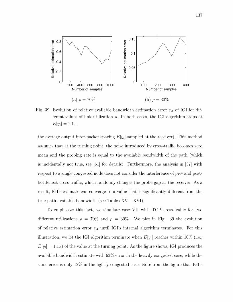
137

200 400 600 800 10000

0.2

0.4

0.6

0.8

Number of samples

Rel

ativ

e es

timat

ion

erro

r

(a) ρ = 70%

100 200 300 4000

0.05

0.1

0.15

Number of samples

Rel

ativ

e es

timat

ion

erro

r

(b) ρ = 30%

Fig. 39. Evolution of relative available bandwidth estimation error eA of IGI for dif-

ferent values of link utilization ρ. In both cases, the IGI algorithm stops at

E[yi] = 1.1x.

the average output inter-packet spacing E[yi] sampled at the receiver). This method

assumes that at the turning point, the noise introduced by cross-traffic becomes zero

mean and the probing rate is equal to the available bandwidth of the path (which

is incidentally not true, see [61] for details). Furthermore, the analysis in [37] with

respect to a single congested node does not consider the interference of pre- and post-

bottleneck cross-traffic, which randomly changes the probe-gap at the receiver. As a

result, IGI’s estimate can converge to a value that is significantly different from the

true path available bandwidth (see Tables XV – XVI).

To emphasize this fact, we simulate case VII with TCP cross-traffic for two

different utilizations ρ = 70% and ρ = 30%. We plot in Fig. 39 the evolution

of relative estimation error eA until IGI’s internal algorithm terminates. For this

illustration, we let the IGI algorithm terminate when E[yi] reaches within 10% (i.e.,

E[yi] = 1.1x) of the value at the turning point. As the figure shows, IGI produces the

available bandwidth estimate with 63% error in the heavily congested case, while the

same error is only 12% in the lightly congested case. Note from the figure that IGI’s

138

0 1000 2000 3000 4000 50000

0.2

0.4

0.6

0.8

1

1.2

Number of samples

Rel

ativ

e es

timat

ion

erro

r

(a) ρ = 70%

200 400 600 8000

0.05

0.1

0.15

0.2

0.25

Number of samples

Rel

ativ

e es

timat

ion

erro

r

(b) ρ = 30%

Fig. 40. Evolution of relative available bandwidth estimation error eA of IGI for dif-

ferent values of link utilization ρ. In both cases, the IGI algorithm stops at

E[yi] = 1.001x.

estimates keep fluctuating until the internal algorithm stops at E[yi] = 1.1x and the

error is not necessarily decreasing over time.

To further investigate IGI’s convergence behavior, we run the IGI algorithm until

it terminates at E[yi] = 1.001x (recall that the turning point means E[yi] = x). We

plot the evolution of relative estimation errors for those two cases with ρ = 70% and

ρ = 30% in Fig. 40. Observe from the figure that even though the initial packet

spacing x becomes closer and closer to the turning point, IGI’s estimation accuracy

significantly fluctuates (between 18% and 122% of relative error) in case of ρ = 70%,

while for ρ = 30%, it gets worse without showing a sign of convergence. This high

variation of IGI’s estimates for different values of x/E[yi] explains extremely high

error in certain path configurations (case IV in Table XVI) and makes it difficult to

decide when to stop IGI’s internal algorithm to produce bandwidth estimates. In the

figure, IGI produces the best estimate some time before it reaches the turning point

and thereafter the accuracy becomes worse as the initial spacing becomes closer to the

139

turning point. Hence, unlike Envelope, using more samples in IGI does not necessarily

lead to better estimation accuracy (for this reason, we let the IGI algorithm terminate

at E[yi] = 1.1x to produce its available bandwidth estimates discussed in Section F.4).

2. CapProbe

Recall that CapProbe is based on the assumption that if packets in a probe pair have

arrived at the receiver with the smallest combined one-way delay, then the packets

have not been queued at any intermediate routers in the path and thus the inter-packet

delay of the probe pair reflects the transmission delay of the bottleneck link. Based

on this assumption, CapProbe uses 100 samples and the minimum delay condition

to obtain the packet-pair that contains information about C. However, CapProbe’s

minimum filtering is sensitive to random queuing delays in front of the first packet of

the pair and thus it is possible that the estimated capacity converges to a value that

is very different from the true value of C. Furthermore, the convergence is rather

random, which makes it difficult, if not impossible, to decide the optimal number of

samples to be used in the estimation algorithm.

To illustrate the queuing effects discussed above, we simulate case VII with TCP

cross-traffic for varying link utilization ρ between 30% and 70%. Fig. 41(a) shows

CapProbe’s relative capacity estimation errors eC for different ρ. Observe that as ρ of

the path increases from 30% to 70%, the relative estimation error eC jumps from 0%

to 48%. This indicates that CapProbe performs very well in a lightly utilized path;

however, in a heavily-congested path, its capacity estimation accuracy significantly

degrades. Furthermore, CapProbe’s estimation accuracy fluctuates substantially de-

pending on the number of samples used as illustrated in Fig. 41(b). For example,

in a path with ρ = 80%, eC = 30% with 100 samples, 47% with 500 samples, 14%

with 1000 samples, and 47% with 3000 samples. This indicates that if the measur-

140

0.3 0.4 0.5 0.6 0.70

0.1

0.2

0.3

0.4

0.5

Link utilization ρ

Rel

ativ

e es

timat

ion

erro

r

(a) eC for different ρ

0 5000 10000

0.1

0.2

0.3

0.4

0.5

0.6

Number of samples

Rel

ativ

e es

timat

ion

erro

r

(b) Evolution of eC

Fig. 41. (a) Relative estimation error eC of CapProbe for different utilization ρ of the

links in case VII. (b) Evolution of relative capacity estimation error eC of

CapProbe for ρ = 80%.

ing process stops at a random plateau where CapProbe has seemingly converged, its

estimation accuracy will be random as shown in Fig. 41(b).

H. Impact of Probing Parameters in Envelope

Recall that Envelope’s bandwidth estimation relies on two sets of measurements,

which sample cross-traffic statistics at routers along the path using alternate probe-

trains. In Envelope, there are two important and controllable parameters: initial

input spacing x and probe-train length N . We discuss their impact on estimation

accuracy of Envelope.

1. Initial Spacing

As discussed in Section F.1, Envelope’s parameter selection routine sets xa as small

as possible to maximize the number of measurable non-tight links, while keeping

xb = q/ADR. Note that Envelope can use smaller xb as long as it is larger than

141

xa, which potentially increases the number of measurable non-tight links. We next

answer the question whether reducing xb (while keeping the same time span xbNb by

increasing Nb) affects estimation accuracy and if so, what impact it has on it.

Define ρk = λk/Ck to be the utilization of router Rk, where Ck is the capacity of

Rk and λk is an average cross-traffic rate arriving at Rk. Recall that W an,k and W b

n,k

are respective n-sample averages of inter-departure spacings yai,k and yb

i,k of router Rk

sampled at the receiver. Define W ak = limn→∞ W a

n,k and W bk = limn→∞ W b

n,k. Assume

that router Rk is measurable. Then, it is easy to obtain ρk from (130) and (133):

ρk =W b

k −W ak

W bk−1 −W a

k−1

. (142)

With finite n, what we really sample at the receiver includes some measurement

noise. Define measurement errors εak = W a

k −W an,k and εb

k = W bk −W b

n,k. Assume that

when link k is examined, W ak−1 and W b

k−1 for the previous router k − 1 are known.

Then, denoting by ρk an estimate of link utilization ρk, we have:

ρk = ρk +εb

k − εak

W bk−1 −W a

k−1

. (143)

Note that the second term in (143) represents the measurement noise in esti-

mation of ρk. Since sampling noise εbk depends on the time span of a probe train

xbNb, the numerator in (143) will be roughly the same regardless of the value of xb

as long as the time span xbNb is maintained the same. Hence, measurement noise

in (143) mainly depends on the difference between two output dispersions W bk−1 and

W ak−1. Also, note from (130) that an average inter-packet dispersion E[yi,k] exiting

from router Rk is non-decreasing as k increase, which results in that a larger input

spacing tends to produce a larger average dispersion from a router than that with

a smaller input spacing. Hence, reducing xb is likely to produce smaller output dis-

persion Wk−1, which in turn leads to higher measurement noise in estimation of link

142

utilization ρk.

To confirm our intuition discussed above, we conduct simulations with xaNa =

36.4 ms and xbNb = 268 ms for two different values of xb = 24.4 ms (Nb = 11) and

xb = 1.92 ms (Nb = 140) using case VII. In measuring the tight link (i.e., router

R3 in this example), the value of metric εb3 − εa

3 is 35 µs for larger xb = 24.4 ms

and 35.8 µs for smaller xb = 1.92 ms, both of which are almost identical. However,

the denominator W b2 −W a

2 is drastically different for two values of xb. For instance,

the denominator is 9.44 ms for the larger xb and 0.39 ms for the smaller xb, which

results in only 0.44% error in estimation of ρ for the former case. However the same

estimation error increases to 10% when smaller xb is used.

In summary, the above result on selection of xb implies that using smaller xb can

potentially degrade estimation accuracy in certain network configurations, while in-

creasing the number of measurable non-tight links in a path. We note that adjusting

xb for each link can improve accuracy; however, it is not applicable to Envelope with-

out significantly increasing measurement overhead since it requires inter-departure

spacings at the previous link k − 1 to measure the current link k.

2. Probe-Train Length

We next study how the probe-train length N affects the estimation accuracy of Enve-

lope. For this example, we disable the automatic parameter selection routine in En-

velope and manually set xa = q/C0 = 0.12 ms and xb = 2 ms. Further set Nb = Na/2

and n = 5Na so that Nb and n are scaled up as Na increases. We then conduct

simulations using case I under TCP cross-traffic for different probe-train length Na

and plot relative estimation errors eC and eA of the tight link in Fig. 42. As the

figure shows, the estimation accuracy of Envelope is improved as probe-train length

Na increases. For example, Envelope produces the bottleneck capacity estimate with

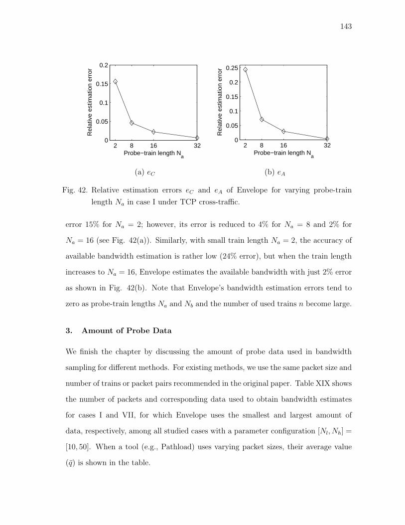
143

2 8 16 320

0.05

0.1

0.15

0.2

Probe−train length Na

Rel

ativ

e es

timat

ion

erro

r

(a) eC

2 8 16 320

0.05

0.1

0.15

0.2

0.25

Probe−train length Na

Rel

ativ

e es

timat

ion

erro

r

(b) eA

Fig. 42. Relative estimation errors eC and eA of Envelope for varying probe-train

length Na in case I under TCP cross-traffic.

error 15% for Na = 2; however, its error is reduced to 4% for Na = 8 and 2% for

Na = 16 (see Fig. 42(a)). Similarly, with small train length Na = 2, the accuracy of

available bandwidth estimation is rather low (24% error), but when the train length

increases to Na = 16, Envelope estimates the available bandwidth with just 2% error

as shown in Fig. 42(b). Note that Envelope’s bandwidth estimation errors tend to

zero as probe-train lengths Na and Nb and the number of used trains n become large.

3. Amount of Probe Data

We finish the chapter by discussing the amount of probe data used in bandwidth

sampling for different methods. For existing methods, we use the same packet size and

number of trains or packet pairs recommended in the original paper. Table XIX shows

the number of packets and corresponding data used to obtain bandwidth estimates

for cases I and VII, for which Envelope uses the smallest and largest amount of

data, respectively, among all studied cases with a parameter configuration [Nl, Nh] =

[10, 50]. When a tool (e.g., Pathload) uses varying packet sizes, their average value

(q) is shown in the table.

144

Table XIX. Bandwidth Sampling Overhead for Cases I and VII

Methods Case-I Case-VII# packets q (B) data (MB) # packets q (B) data (MB)

Envelope [10, 50] 4, 692 1, 500 7.0 9, 376 1, 500 14.0[5, 15] 2, 668 1, 500 4.0 3, 540 1, 500 5.3

Pathrate 28, 440 1, 500 42.7 15, 440 1, 500 23.1CapProbe 200 800 0.2 400 800 0.3Pathload 15, 600 513 8.0 14, 400 207 3.0Spruce 4, 000 1, 500 6.0 4, 000 1, 500 6.0

IGI 360 700 0.3 780 700 0.5

As the table shows, IGI and CapProbe do not use many samples, while Pathload,

Pathrate, and Envelope requires significantly more probe packets for their measure-

ment. For example, Pathload uses 15600 samples for case I and 14400 samples for case

VII, which accounts to 3 − 8 MB of data. In Pathrate, cases I and VII respectively

use 42 MB and 23 MB of samples to produce bottleneck bandwidth estimates. Note

that when high values for Nl and Nh, i.e., [Nl, Nh] = [10, 50], are used, Envelope uses

7 MB of probe packets for case I and 14 MB for case VII (see column 3 in the table).

However, with smaller values of [Nl, Nh] = [5, 15], the amount of used data is reduced

to 4 MB for case I and 5 MB for case VII (see column 4 in the table). Recall that

Envelope can also measure some non-tight links in certain network settings. For in-

stance, it is able to measure the first three links in case VII, while it can only measure

the tight link in case I. Hence, even with [Nl, Nh] = [10, 50], per-hop measurement

overhead in Envelope is 7 MB for case I and 4.6 MB for case VII, which are similar

to those in Pathload for both cases (note that Pathload can only measure the tight

link).

Also, recall that the number of samples required for Envelope is proportional

to the number of hops in the path. Thus, for a 10-hop Internet path and using

145

[Nl, Nh] = [10, 50], Envelope needs 17−35 MB of probe data to examine all individual

links. With smaller values of parameter configuration [5, 15], it requires 10− 13 MB

of data for the same 10-hop Internet path.

146

CHAPTER VI

ROBUST BANDWIDTH MEASUREMENT OF

END-TO-END PATHS

In this chapter, we investigate the problem of end-to-end bandwidth estimation under

realistic environment. Recall that existing approaches can be classified into measure-

ment tools [22], [37], [41], [43], [49], [54], [72], [96], which usually have extensive sim-

ulations, but no convergence analysis for general cross-traffic, and theoretical models

[34], [48], [60], [61], [62], [69], [75], which usually have provable convergence, but no

practical implementation. Another issue in related work is the unknown performance

of certain proposed algorithms in real networks where delay measurements are not

perfect due to various OS and hardware-related timing irregularities [81]. We address

the former issue by developing a measurement tool PRC-MT based on the models of

[61] that not only achieves asymptotic accuracy in multi-path networks with arbitrary

cross-traffic, but also simultaneously measures the capacity and available bandwidth

of the tight link. We address the latter issue by performing a comparison study of

existing tools in Emulab/PlanetLab and assessing their susceptibility to timing ir-

regularities of end-hosts. Our results show that PRC-MT outperforms all existing

tools in terms of accuracy, achieves similar convergence delay, and does not require

any manual configuration. We also find that interrupt moderation may cause existing

tools (such as Pathload [43], Pathchirp [85], and CapProbe [49]) to become quite in-

accurate in certain network configurations and exhibit behavior completely different

from that in ns2 [92].

147

A. Introduction

Bandwidth of Internet paths is an important metric for many applications. However,

without a direct access to network resources, end-to-end bandwidth measurement

under general conditions on cross-traffic is a rather complex process [34], [61]. Unfor-

tunately, theoretically justified techniques [61], [69], [75] are commonly not available

as practical tools that can be used in real networks and vice versa (i.e., existing im-

plementations are often based on fluid models that exhibit bias in bursty networks

[61] and/or rely on heuristics with unknown theoretical performance). In addition,

many current techniques produce unreliable results in actual networks where packet

dispersions cannot be sampled accurately due to hardware interrupt moderation and

various OS-imposed overhead [81].

1. Measuring the Tight Link

Existing techniques usually estimate either the available bandwidth [37], [44], [85], [96],

or the bottleneck bandwidth [22], [49] of the path. The former term refers to the unused

bandwidth At of the tight link (i.e., link with the smallest available bandwidth) and

is closely related to the rate at which new applications can send into the path without

congesting it. The latter metric is the capacity Cn of the narrow link (i.e., link with

the lowest speed), which can be viewed as an upper bound on the sending rate that

the path can support. Note that At can be measured in all network configurations,

while this is not necessarily true for Cn.

Even though both At and Cn are useful metrics, certain applications require ca-

pacity Ct of the tight link instead of Cn, which allows them to compute the utilization

of the tight link and possibly achieve better characterization of what causes bottle-

148

necks in the path.1 Only a few approaches can measure Ct [47], [48], [72], but they are

either based on single-hop models that are inaccurate in multi-path networks, or rely

on hop-by-hop probing, which we do not study in this chapter. A recent theoretical

development [61] shows that both At and Ct can be provably measured in any end-

to-end path with infinite buffers by exploiting a certain piece-wise linear relationship

between the sending rate rI of probe packets and the corresponding arrival rate rO at

the receiver. Although this work opens a door for developing a new characterization

technique for tight links, it remains to be seen if an automated implementation can

achieve good performance in networks with limited buffer space and exhibit overhead

comparable to that of existing tools.

Recall that [61] relies on correctly identifying the first two linear segments of the

probing response curve (PRC), which is a functional relationship between rI/rO and

rI . Identifying and separating the linear segments in a stochastic PRC is a non-trivial

task since the curve itself may fluctuate and/or deviate from the fluid piece-wise linear

limit depending on path-specific characteristics as well as the number of probes per

train and their size. In addition, building an entire PRC sometimes requires sending a

large amount of traffic into the path and exhaustively probing a wide variety of sending

rates (i.e., as done in [63]). Thus, the main challenge in PRC-based estimation is the

development of automated algorithms for detecting linear segments in practice and

selecting probing rates that result in quick convergence of the method.

In this chapter, we tackle the above problems in an iterative probing technique

we call PRC Measurement Tool (PRC-MT), which is capable of estimating both At

and Ct in arbitrary multi-hop paths. PRC-MT autonomously selects probing rates,

train and packet size, and termination conditions so as to achieve any desired tradeoff

1Also note that certain bandwidth estimation tools [36], [96] require Ct in orderto measure At.

149

between accuracy and overhead (i.e., better accuracy requires more probes and vice

versa). We implement PRC-MT in Linux and evaluate its performance in a network

of software routers of Emulab. We find that PRC-MT, limited to the execution delay

of prior methods (i.e., 90−120 seconds), estimates At and Ct with 90−99% accuracy

in a wide range of network configurations.

2. Timing Irregularities

Attempting to run existing tools in PlanetLab, we found that some of them frequently

produced no estimate at all (e.g., Pathload [43], [44]) while others returned results that

did not make much sense (e.g., CapProbe [49]). It became immediately clear that one

of the main factors that differentiates bandwidth estimation in real networks from that

in ns2 is end-host timing irregularities, which include hardware interrupt moderation

[81] and OS scheduling delay jitter (which depends on the CPU utilization of the

host). We sampled a number of hosts in PlanetLab and found that many of them

used interrupt moderation, which could be enabled at the sender (i.e., packets did

not leave the host immediately), at the receiver (i.e., arriving packets were delivered

to the OS “bunched up”), or at both. In fact, modern gigabit NICs enable interrupt

moderation by default, which means that bandwidth-measurement tools that are not

robust to timing irregularities are unlikely to be successful in real networks.

To reduce the effect of interrupt moderation, techniques such as Pathchirp [85]

and the current version of Pathload [44], [81] incorporate mechanisms that aim to

“weed out” packets affected by interrupt delays. Specifically, Pathchirp requires

manual modification to force it to send more probing packets to obtain an accu-

rate estimate. For Emulab experiments in this chapter, we use 6 times more packets

per probing train (i.e., chirp) than the default value in order to achieve reasonable

accuracy. This modification reduces the effect of interrupt delay, but prolongs the

150

measurement. On the other hand, Pathload attempts to filter out affected packets

without increasing the number of probing packets, which unfortunately has a limited

effect when interrupt delays become non-trivial. This makes Pathload’s estimation

much more susceptible to error, which happens fairly often in practice.

In order to obtain a working version of Pathload that can be used in our com-

parison with PRC-MT in scenarios with non-negligible interrupt delays, we inves-

tigate Pathload’s internal algorithm and find that its estimation instability stems

from its delay-trend detection mechanism that is not robust under bursty packet

arrival introduced by network hardware. To overcome this problem, we introduce

two trend-detection algorithms based on signal de-noising techniques and show that

they significantly improve Pathload’s performance in real networks. We call the new

method Interrupt Moderation Resilient Pathload (IMRP) and show that it not only

outperforms the original Pathload, but also achieves better estimation accuracy than

Pathchirp under a wide range of interrupt delay δ, while using approximately half the

time and 75% less bandwidth.

We next assess the performance of PRC-MT under interrupt moderation in com-

parison with IMRP, Pathchirp [85], IGI/PTR [36] using metric At and Pathrate [22],

CapProbe [49] using metric Ct when the narrow link coincides with the tight link.

For available bandwidth At, our results show that PRC-MT exhibits no negative

side-effects related to interrupt moderation, converges in 90 − 140 seconds in all ex-

amined topologies, and outperforms the other studied methods in terms of accuracy

(1 − 5% error). We also find that IMRP’s estimates are generally within 7% of the

correct value and its convergence delay is 80− 100 seconds. After manually tweaking

Pathchirp’s train size and running duration, we were able to reduce its error to about

15% and execution time to 200 seconds; however, its default version performs much

worse. Even though we supply IGI/PTR with the correct tight-link capacity Ct, both

151

methods exhibit 40 − 60% error, but on the bright side converge within just 3 − 5

seconds.

For tight-link capacity Ct, PRC-MT’s error is below 7% in all studied cases, while

that of Pathrate exceeds 15% and that of CapProbe is close to 60%. The measurement

delay of prior methods is also significantly higher than that of PRC-MT – almost 2200

seconds in Pathrate and 500 seconds in CapProbe. Our Emulab results suggest that

existing methods (in their unmodified form) may experience certain non-negligible

performance issues in real networks, while techniques introduced in this work (PRC-

MT and IMRP) are much more likely to remain robust in practical settings. In fact,

PRC-MT not only provides automatic self-configuration that overcomes interrupt-

moderation effects and achieves quick convergence, but also simultaneously estimates

(At, Ct) and is asymptotically accurate. We finish the chapter by measuring two paths

in PlanetLab [80] using all 8 studied tools and discussing their possible inaccuracies.

B. PRC-MT: Bandwidth Estimation Using Probing Response Curve

In this section, we investigate practical issues and difficulties of using PRC in mea-

suring available bandwidth and capacity of the tight link. We then develop empirical

algorithms that overcome these problems and lead to a new measurement tool called

PRC-MT, which can measure both bandwidth metrics of the tight link over multi-hop

paths under arbitrary cross-traffic and routing patterns. We start by describing the

basic idea of this approach.

1. Basic Idea

Define rI to be a sending rate of packets in a probe-packet train at the sender and

rO to be their arrival rate at the receiver. Further define F = rI/rO to be the ratio

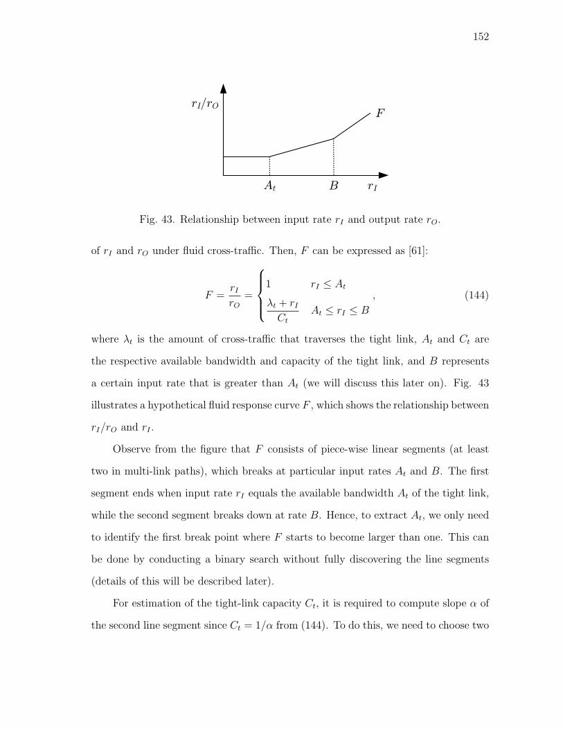
152

At B rI

rI/rOF

Fig. 43. Relationship between input rate rI and output rate rO.

of rI and rO under fluid cross-traffic. Then, F can be expressed as [61]:

F =rI

rO

=

1 rI ≤ At

λt + rI

Ct

At ≤ rI ≤ B

, (144)

where λt is the amount of cross-traffic that traverses the tight link, At and Ct are

the respective available bandwidth and capacity of the tight link, and B represents

a certain input rate that is greater than At (we will discuss this later on). Fig. 43

illustrates a hypothetical fluid response curve F , which shows the relationship between

rI/rO and rI .

Observe from the figure that F consists of piece-wise linear segments (at least

two in multi-link paths), which breaks at particular input rates At and B. The first

segment ends when input rate rI equals the available bandwidth At of the tight link,

while the second segment breaks down at rate B. Hence, to extract At, we only need

to identify the first break point where F starts to become larger than one. This can

be done by conducting a binary search without fully discovering the line segments

(details of this will be described later).

For estimation of the tight-link capacity Ct, it is required to compute slope α of

the second line segment since Ct = 1/α from (144). To do this, we need to choose two

153

points on the second line segment, which may not be easy to identify without knowing

the exact rate B of the second break point. Recall from [61] that B is dependent on

the routing matrix of cross-traffic traversing the path and thus it is not possible to

compute its value without complete knowledge of cross-traffic routing patterns. What

we know is that B is no less than the second smallest hop-available bandwidth of the

path. Judging from this lack of knowledge on B, extracting Ct appears to be harder

than finding At and be more susceptible to measurement errors.

Now the question we have is how to find the first break point for estimation of

At and how to identify the second line segment and compute its slope α for capacity

estimation without even knowing the exact value of B in practice. We address these

issues in the following subsections.

2. Issues

Define Z to be the real probing response curve of a path over which arbitrarily routed

bursty cross-traffic flows traverse. Note that Z is different from the fluid curve F (as

long as probe-train length N and probe-packet size q are finite) and this makes the

task of identifying the first break point and the second linear segment in Z significantly

more challenging than that in the fluid case. Although it is proven in [61] that Z is

lower-bounded by fluid response curve F and asymptotically approaches F as N →∞or q →∞, Z−F > 0 in real networks, where the size of packets is typically limited by

the maximum transfer unit (MTU) of network elements and the packet-train length

N cannot be arbitrarily large since router queue sizes are limited.

Before discussing implications of this deviation of Z from F , we explore how

the response curve Z behaves with different probe-train length N by conducting

experiments in Emulab and ns2 [73] using a single-hop topology of capacity Ct = 90

Mb/s. For this experiment, we keep link utilization at 32% (i.e., λt = 29 Mb/s) and

154

58 60 62 64 66

1

1.05

1.1

1.15

Input probe rate rI

Rat

io r

I/rO

N=15N=60N=240fluid bound

Fig. 44. Probing response curves for different values of probe-train length N in Emulab

experiments.

plot the response curve Z for several different values of N in Fig. 44.

Notice in Fig. 44 that when N is small (e.g., 15), Z fluctuates substantially

and exhibits large deviation from the fluid lower-bound F . However, as N increases,

Z shows prominent two linear lines and its deviation from F becomes smaller. For

example, with N = 240, rO is within 1.5% of rI until rI reaches around 61 Mb/s,

which is the available bandwidth At of the path in this setup. Note that the difference

between Z and F would be zero as N becomes large (we do not show this since we

cannot use arbitrarily large N in Emulab without causing packet loss due to queue

size limit).

To better demonstrate behavior of Z for a large probe-train length N , we conduct

ns2 simulations for different N with two different probe-packet sizes q = 1500 and

200 bytes. As shown in Fig. 45(a), although Z deviates from F with N = 15, it

converges to F when N = 240, which in general agrees with the Emulab result in Fig.

44. Note that the simulation result in Fig. 45(a) shows less variation in Z and faster

convergence of Z to F, which we believe stems from perfect timestamping of sending

and arriving packets in ns2. With smaller packets (e.g., q = 200 bytes), we observe

a similar behavior of Z even though it exhibits higher fluctuation and requires larger

155

58 60 62 64 66

1

1.05

1.1

Input probe rate rI

Rat

io r

I/rO

N=15N=240fluid bound

(a) ns2 (q = 1500 B)

58 60 62 64 66

1

1.05

1.1

1.15

Input probe rate rI

Rat

io r

I/rO

N=60N=480fluid bound

(b) ns2 (q = 200 B)

Fig. 45. Probing response curves for different probe-train length N in ns2 simulation.

N to converge to F (see Fig. 45(b)).

Next, we discuss how the evolution of the real response curve Z on input probe

rate rI affects bandwidth estimation. Recall that to estimate bandwidth At and Ct,

we need to identify the end of the first line segment (for At) and stable second linear

line (for Ct) from the response curve Z. For accurate discovery of the first break

point in Z, it is required that variation in Z should be small for different rI . More

importantly, it is desired to have a second line segment that is parallel to that in F

even though they do not match (i.e., deviation Z − F > 0). Note that if the second

line segments in Z and F are parallel, then we can use any two points on the line

in Z to compute its slope α, which reflects the true capacity Ct of the tight link

regardless of their locations as long as they are on the second line segment. Further

note that under this condition the amount of deviation Z − F has no direct impact

on estimation accuracy. However, if the second line segment in Z is not parallel to

that of fluid counter part F , then estimation accuracy of Ct depends on which two

points we select in computing the slope α, which is a non-trivial task in practice.

To confirm the above discussion and demonstrate the direct impact of the probe-

train length N on estimation accuracy, we conduct experiments in Emulab using the

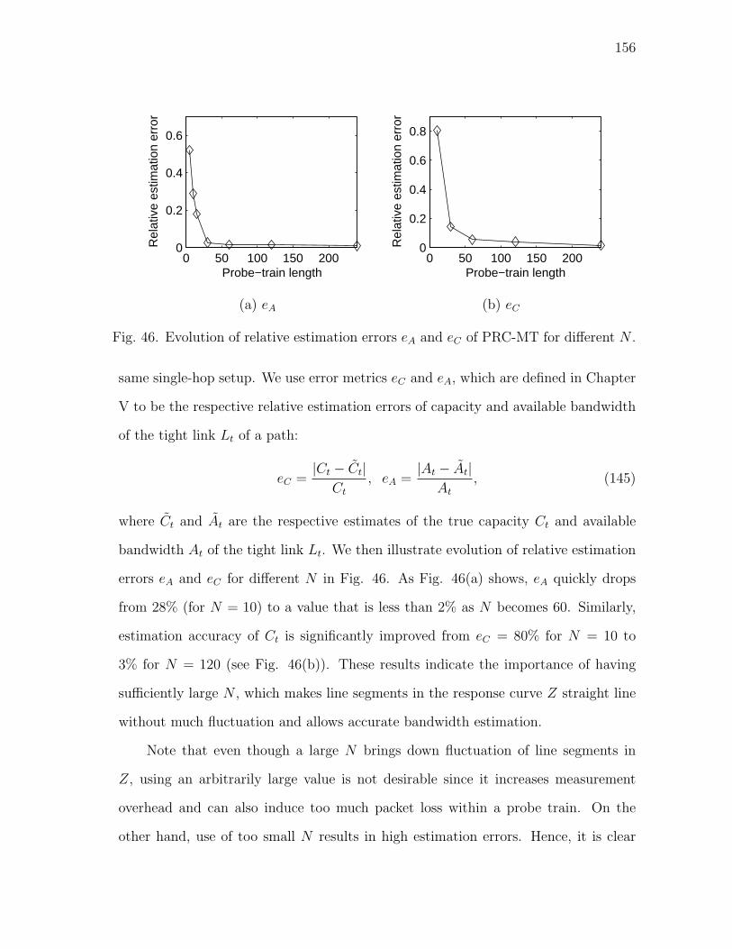
156

0 50 100 150 2000

0.2

0.4

0.6

Probe−train length

Rel

ativ

e es

timat

ion

erro

r

(a) eA

0 50 100 150 2000

0.2

0.4

0.6

0.8

Probe−train length

Rel

ativ

e es

timat

ion

erro

r

(b) eC

Fig. 46. Evolution of relative estimation errors eA and eC of PRC-MT for different N .

same single-hop setup. We use error metrics eC and eA, which are defined in Chapter

V to be the respective relative estimation errors of capacity and available bandwidth

of the tight link Lt of a path:

eC =|Ct − Ct|

Ct

, eA =|At − At|

At

, (145)

where Ct and At are the respective estimates of the true capacity Ct and available

bandwidth At of the tight link Lt. We then illustrate evolution of relative estimation

errors eA and eC for different N in Fig. 46. As Fig. 46(a) shows, eA quickly drops

from 28% (for N = 10) to a value that is less than 2% as N becomes 60. Similarly,

estimation accuracy of Ct is significantly improved from eC = 80% for N = 10 to

3% for N = 120 (see Fig. 46(b)). These results indicate the importance of having

sufficiently large N , which makes line segments in the response curve Z straight line

without much fluctuation and allows accurate bandwidth estimation.

Note that even though a large N brings down fluctuation of line segments in

Z, using an arbitrarily large value is not desirable since it increases measurement

overhead and can also induce too much packet loss within a probe train. On the

other hand, use of too small N results in high estimation errors. Hence, it is clear

157

that there exists a trade-off between accuracy and overhead and thus proper selection

of train length N is very important in developing PRC-MT. However, selection of

appropriate value of N is non-trivial since fluctuation of line segments in the real

response curve Z depends on probe parameters and unknown path characteristics

such as amount of cross-traffic.

Now, the problem we need to solve is how to select N in practice for a particular

path such that the second line segment in Z becomes parallel to that in F . We

investigate this next.

3. Parameter Selection

Recall that for a sufficiently large N , the slope of the second line segment in Z

converges to a value that makes it parallel to that of fluid curve F in an input rate

range rI ∈ [At, B]. We can interpret this as that the ratio rI/rO saturates at a certain

value when N becomes large. To confirm this, we examine the quantity of rI/rO for

different N using the Emulab setup discussed in the previous subsection. For this

purpose, we send packets with rate rI = 68 Mb/s (which is higher than the available

bandwidth At = 61 Mb/s of the path in this setup) with varying N and plot rI/rO

in Fig. 47. As the figure shows, rI/rO quickly drops to a value that is slightly larger

than the fluid-bound (i.e., (λt + rI)/Ct = 1.07) as N increases. This leads us to

investigating an empirical method, which iteratively probes for N that makes the

ratio rI/rO saturate for a given input rate rI .

In what follows below in this section, we discuss a simple selection procedure

for N , which adjusts its value based on variation of rI/rO for a given sending rate

rI discussed above. Although there is no particular constraints on the input sending

rate for this routine, it is preferable to use a rate that is not so smaller than available

bandwidth At of the path since variation of the ratio rI/rO for an input rate that is

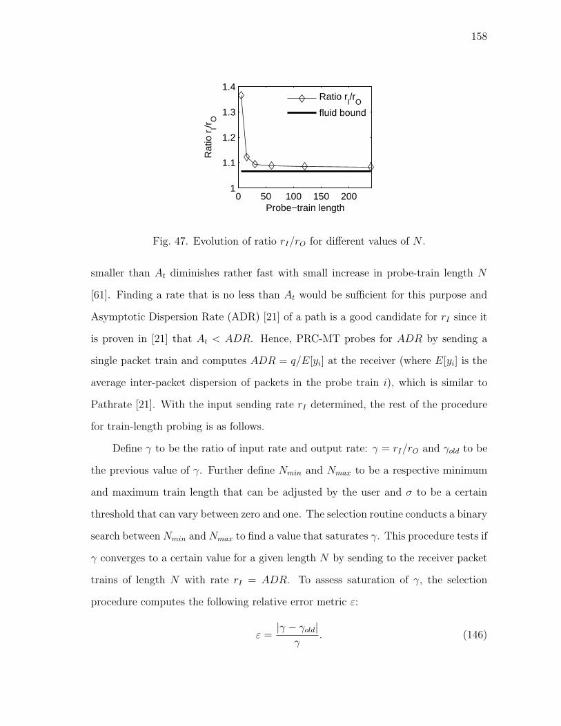
158

0 50 100 150 2001

1.1

1.2

1.3

1.4

Probe−train lengthR

atio

rI/r

O

Ratio rI/r

O

fluid bound

Fig. 47. Evolution of ratio rI/rO for different values of N .

smaller than At diminishes rather fast with small increase in probe-train length N

[61]. Finding a rate that is no less than At would be sufficient for this purpose and

Asymptotic Dispersion Rate (ADR) [21] of a path is a good candidate for rI since it

is proven in [21] that At < ADR. Hence, PRC-MT probes for ADR by sending a

single packet train and computes ADR = q/E[yi] at the receiver (where E[yi] is the

average inter-packet dispersion of packets in the probe train i), which is similar to

Pathrate [21]. With the input sending rate rI determined, the rest of the procedure

for train-length probing is as follows.

Define γ to be the ratio of input rate and output rate: γ = rI/rO and γold to be

the previous value of γ. Further define Nmin and Nmax to be a respective minimum

and maximum train length that can be adjusted by the user and σ to be a certain

threshold that can vary between zero and one. The selection routine conducts a binary

search between Nmin and Nmax to find a value that saturates γ. This procedure tests if

γ converges to a certain value for a given length N by sending to the receiver packet

trains of length N with rate rI = ADR. To assess saturation of γ, the selection

procedure computes the following relative error metric ε:

ε =|γ − γold|

γ. (146)

159

When ε ≤ σ, the routine decreases N ; otherwise, it increases N .

Note that users can use any packet size qmin ≤ q ≤ qmax (where we use qmin = 200

bytes and qmax = 1500 bytes), in which case Nmin and Nmax are scaled up or down

by qmax/q. This routine ensures us to select a larger N when a user chooses a smaller

packet q, sufficing the condition for stabilizing line segments in Z as discussed in

the previous subsection. For experiments in Sections C. and D., we use Nmin = 60,

Nmax = 3000, σ = 0.02, and q = 200 bytes.

4. Bandwidth Probing

With probe-train length N in hands, our next question is how to identify the first

break point in the response curve Z, at which input sending rate rI starts to become

larger than the arrival rate rO (see Fig. 43). To efficiently search for this point,

PRC-MT uses an iterative probing-based binary search, which is similar to Pathload

[44]. Note, however, that the two tools are different in a way that assesses whether

an input rate rI corresponds to At. For example, PRC-MT determines if the current

rate rI > At by directly comparing rI with rO, while Pathload infers it by examining

one-way delays of probe packets.

Similarly to Pathload, PRC-MT sends a group of K packet trains with a given

rate rI . Then, based on how much fraction η of K trains belongs to either rI > rO

or rI < rO, it adjusts its sending rate rI . Specifically, PRC-MT decrease rI if a

fraction η of K probe-trains are asserted to be rI > rO; increase rI when the ratio

of the number of trains with rI < rO to K is more than η. Note that it is possible

that neither of the above two cases happens (i.e., none of ηK trains belongs to either

rI > rO or rI < rO). If this is the case, we treat it like a “grey region” in Pathload

(see [44] for details).

This binary search process continues until the bandwidth range [WL,WH ] around

160

At becomes smaller than a certain threshold ω, which can be automatically selected

(ω = 0.02ADR) based on measured ADR or given by the user. PRC-MT returns

At = (WL + WH)/2 as the available bandwidth estimate of the tight link when its

internal algorithm terminates. We empirically set η = 60% and K = 12 as their

respective default value in PRC-MT.

After finding a bandwidth range [WL,WH ], PRC-MT starts a procedure for es-

timating the tight-link capacity Ct. The main focus of this routine is to select two

points that will be used to extract Ct without the knowledge of the end of the second

line segment. Note that to facilitate estimation of Ct, PRC-MT records the sending

rate rI and its corresponding receiving rate rO during the available bandwidth prob-

ing whenever the current rI reduces the upper bound WH of the bandwidth range

due to rI being larger than rO. These recorded points are the possible candidates for

computing a capacity estimate Ct.

Note that we can select any two among the recorded points to extract Ct in ideal

case (i.e., the second segment is a perfect straight line and there is no measurement

noise). Unfortunately, however, there is no straightforward method that chooses

optimal two points with certain measurement noise and imperfect straight line, which

leads us to exploring empirical method (which we explain below).

Assume that there are m ≥ 2 recorded points (u1, v1), . . . , (um, vm), where ui

and vi (i = 1, . . . , m) are the respective sending and receiving rates used during the

available bandwidth probing. Then, PRC-MT first chooses (ui, vi), where ui is the

smallest among m points that satisfies ui ≥ WH . We have two reasons for not using

rI = At as the first point. First, it is not very clear from the response curve Z where

the second line segment starts around At (see Fig. 44). The other reason is that

the estimated value At may be on the first line segment due to measurement error

(A < At), which can result in high errors in capacity estimation.

161

Recall that to produce accurate capacity estimates Ct, the second point should

be on the second line segment. Since PRC-MT picks the first point (ui, vi) whose

sending rate ui is closest to WH among recorded points, we may consider the point

that is close to the first one as the best candidate for the second point since it has

higher chance to be on the second line segment. However, if two points are close

to each other, then computing linear slope of the two points is more susceptible to

measurement noise. Hence, it is better to have the second point as far away as possible

from the first one as long as they are on the second line segment. Since there is no

way to determine the end of the second line segment, we empirically select farthest

two points among the recorded points to extract the tight-link capacity. Based on the

above discussion, PRC-MT uses (uj, vj) as the second point, where uj is the largest

among the recorded points.

Having two points (ui, vi) and (uj, vj) selected, PRC-MT computes the tight-link

capacity estimate Ct:

Ct =vivj(ui − uj)

uivj − ujvi

, (147)

which is the inverse of a slope of the linear line segment between (ui, ui/vi) and

(uj, uj/vj).

Before concluding this section, we should note that if the number of recorded

points m is less than 2, PRC-MT requires to send additional packets with rates rI

that is larger than At to obtain (rI , rO) pairs. Even though this case will rarely

happen (only when a very large threshold ω is used to terminate the algorithm), we

include this for the sake of completeness.

162

C. Performance of PRC-MT

To evaluate the performance of PRC-MT, we conduct experiments in Emulab2 [24].

We examine estimation accuracy of PRC-MT and its convergence behavior and then

compare these results with those in existing methods. For experiments in this section,

we do not use interrupt moderation (i.e., interrupt delay δ = 0) at the receiver

and defer discussion of these tools under interrupt delay to Section D. We start by

describing the experimental setup.

1. Experimental Setup

For all experiments, we use a topology shown in Fig. 48, in which source PS sends

probe data to the destination PR through five routers R1, . . . , R5. Nodes Si (i =

1, 2, 3, 4) send cross-traffic packets to destination nodes Di (i = 1, 2, 3, 4) at an average

rate λi. The speed of all access links is 100 Mb/s (delay 10 ms) and the remaining

links Li (i = 1, 2, 3, 4) between routers Ri and Ri+1 have capacities Ci and propagation

delay 40 ms.

To examine the estimation accuracy of PRC-MT, we use six different network

settings shown in Table XX, which lists the capacity and available bandwidth of each

link for different experimental scenarios. Note that the table shows a fair amount of

cross-traffic at each node, which is needed to ensure that each case represents some

non-degenerate scenario. Without cross-traffic, most studied techniques are accurate

and their comparison is not very insightful. The values in braces in each row represent

the tight-link capacity Ct and available bandwidth At of the path for each case. The

values in square brackets are the capacities Cn of the narrow link (i.e., bottleneck

bandwidth) for each case. Notice from the table that the experimental settings cover

2In Emulab, users can change configuration of network interface cards.

163

R1 R2 R3C1 C2

R4 R5C3 C4

PRPS

S2 D2 S3 D3

S4 D4 D

100 Mb/s

10 ms

100 Mb/s

10 ms

100 Mb/s

10 ms

100 Mb/s

10 ms

100 Mb/s

10 ms

100 Mb/s

10 ms

S1

100 Mb/s

10 ms

100 Mb/s

10 ms

100 Mb/s

10 ms

100 Mb/s

10 ms

Fig. 48. Evaluation topology in Emulab.

Table XX. Evaluation Setup

Different link bandwidths (Mb/s)C1 A1 C2 A2 C3 A3 C4 A4

Case-I {75 31.8} 90 51.6 90 42.1 [60] 40.7Case-II 75 41.3 90 70.7 90 46.7 {[60] 26.4}Case-III [60] 35.8 90 70.7 90 23.4 {75 18.1}Case-IV {[60] 21.6} 90 65.9 90 42.1 75 36.7Case-V [60] 50.2 90 61.1 {90 41.9} 75 50.8Case-VI 75 28.9 90 37.8 {90 13.8} [60] 31.2

all possible relationships between the location of the tight link and narrow link. For

instance, in cases II and IV, the narrow link coincides with the tight link; in cases I

and VI, the narrow link follows the tight link; while in cases III and V, the narrow

link precedes the tight link.

In all experiments, we use TCP cross-traffic generated by the Iperf traffic gen-

erator [40] to load network paths. Although Iperf traffic does not exactly resemble

Internet traffic, it is adequate for our purposes in this chapter. We run 100 threads in

each cross-traffic source Si to generate TCP flows that are injected into routers R1,

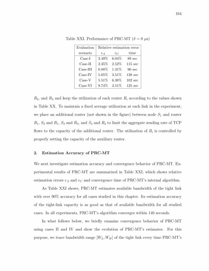
164

Table XXI. Performance of PRC-MT (δ = 0 µs)

Evaluation Relative estimation errorscenario eA eC timeCase-I 3.49% 6.04% 89 secCase-II 2.35% 2.52% 115 secCase-III 0.88% 1.31% 96 secCase-IV 5.05% 3.51% 138 secCase-V 5.51% 6.38% 102 secCase-VI 9.74% 3.51% 125 sec

R2, and R3 and keep the utilization of each router Ri according to the values shown

in Table XX. To maintain a fixed average utilization at each link in the experiment,

we place an additional router (not shown in the figure) between node S1 and router

R1, S2 and R1, S3 and R3, and S4 and R2 to limit the aggregate sending rate of TCP

flows to the capacity of the additional router. The utilization of Ri is controlled by

properly setting the capacity of the auxiliary router.

2. Estimation Accuracy of PRC-MT

We next investigate estimation accuracy and convergence behavior of PRC-MT. Ex-

perimental results of PRC-MT are summarized in Table XXI, which shows relative

estimation errors eA and eC and convergence time of PRC-MT’s internal algorithm.

As Table XXI shows, PRC-MT estimates available bandwidth of the tight link

with over 90% accuracy for all cases studied in this chapter. Its estimation accuracy

of the tight-link capacity is as good as that of available bandwidth for all studied

cases. In all experiments, PRC-MT’s algorithm converges within 140 seconds.

In what follows below, we briefly examine convergence behavior of PRC-MT

using cases II and IV and show the evolution of PRC-MT’s estimates. For this

purpose, we trace bandwidth range [WL,WH ] of the tight link every time PRC-MT’s

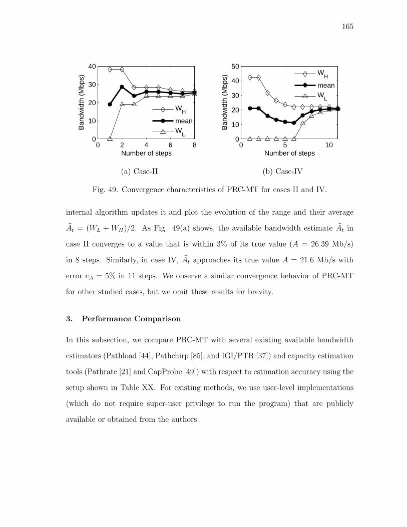
165

0 2 4 6 80

10

20

30

40

Number of steps

Ban

dwid

th (

Mbp

s)

WH

meanW

L

(a) Case-II

0 5 100

10

20

30

40

50

Number of steps

Ban

dwid

th (

Mbp

s)

WH

meanW

L

(b) Case-IV

Fig. 49. Convergence characteristics of PRC-MT for cases II and IV.

internal algorithm updates it and plot the evolution of the range and their average

At = (WL + WH)/2. As Fig. 49(a) shows, the available bandwidth estimate At in

case II converges to a value that is within 3% of its true value (A = 26.39 Mb/s)

in 8 steps. Similarly, in case IV, At approaches its true value A = 21.6 Mb/s with

error eA = 5% in 11 steps. We observe a similar convergence behavior of PRC-MT

for other studied cases, but we omit these results for brevity.

3. Performance Comparison

In this subsection, we compare PRC-MT with several existing available bandwidth

estimators (Pathload [44], Pathchirp [85], and IGI/PTR [37]) and capacity estimation

tools (Pathrate [21] and CapProbe [49]) with respect to estimation accuracy using the

setup shown in Table XX. For existing methods, we use user-level implementations

(which do not require super-user privilege to run the program) that are publicly

available or obtained from the authors.

166

Table XXII. Available Bandwidth Estimation Methods (δ = 0 µs)

Estimation Metrics Evaluation scenariomethod Case-I Case-II Case-III Case-IV Case-V Case-VI

PRC-MT eA 3.49% 2.35% 0.88% 5.05% 5.51% 9.74%time 89 sec 115 sec 96 sec 138 sec 102 sec 125 sec

Pathload eA 9.45% 8% 7.57% 6.48% 16.58% 15.01%time 69 sec 69 sec 70 sec 69 sec 108 sec 99 sec

Pathchirp eA 10.84% 8.53% 0.39% 1.62% 19.81% 18.04%time 200 sec 200 sec 200 sec 200 sec 200 sec 200 sec

IGI eA 10.58% 4.21% 72.76% 19.72% 13.38% 98.56%PTR 16.02% 9.93% 30.28% 24.63% 5.31% 59.24%

time 3 sec 4 sec 5 sec 6 sec 3 sec 5 sec

a. Available Bandwidth Comparison

We first compare PRC-MT with Pathload, Pathchirp, and IGI/PTR. We also have

studied Spruce [96], but do not include its result here since it performs significantly

worse than the other tools in all cases studied in this chapter (see [56], [61] for details

of Spruce and possible causes of its estimation inaccuracy in multi-hop paths).

Table XXII shows relative estimation errors eA for different cases. For Pathload,

we average the low and high values of the produced estimates after its internal algo-

rithm terminates. For Pathchirp, we use “jumbo” option J that increases accuracy

by sending more packets in each probe train (called chirp) than the default. We

manually set this option J = 6 to send 6 times more packets than the default to pro-

duce accurate and reliable available bandwidth estimates. Selection of the value J is

purely based on trial and error since Pathchirp does not offer any automatic selection

mechanism for it. Different from other tools studied in this subsection, Pathchirp

is an open loop system, which does not have an automatic convergence mechanism.

It runs for a specified time t and stops when the running time reaches t, without

167

knowing convergence of its estimate. We use t = 200 seconds to obtain results in this

chapter even though its default execution time is t = 600 seconds since its estima-

tion accuracy has not been improved even we run it more than 200 seconds in our

experimental setup. In IGI/PTR case, we use the estimates available at the end of

its internal convergence algorithm. Note that we feed IGI/PTR the exact tight-link

capacity Ct, while all other tools operate without this information.

As the table shows, Pathchirp produces estimates with less than 20% of error for

all cases. Note that IGI/PTR produces estimates very quickly (40 times faster than

Pathchirp), but its estimation error is significantly higher than Pathchirp. Pathload

measures the paths with accuracy that is similar to Pathchirp. Notice in the table

that PRC-MT produces bandwidth estimates with accuracy that is comparable to or

better than those of Pathload and Pathchirp.

b. Bottleneck Bandwidth Comparison

Note that only in cases II and IV, the narrow link coincides with the tight link

of the path. Hence, we compare PRC-MT only in these path configurations with

recent bottleneck bandwidth estimators CapProbe and Pathrate. For CapProbe, we

use 1800 packet-pairs for estimation since it often does not produce good estimates

(on the studied paths) with 100 pairs recommended in the paper [49]. In Pathrate,

the internal algorithm executes for over 2000 seconds (around 36 minutes) to get

estimates of the bottleneck capacity of the end-to-end path (note that Pathrate has

quick termination mode that takes about 100 seconds, but we do not use this since

its estimate is not accurate in the cases studied in this chapter).

Table XXIII illustrates relative capacity estimation errors eC of the different

methods. As the table shows, PRC-MT produces capacity estimates Ct of the tight

link within 5% of its true values Ct in the studied cases, which is significantly better

168

Table XXIII. Capacity Estimation Methods (δ = 0 µs)

Methods Relative estimation error eC

Case-II Case-IVeC time eC time

PRC-MT 2.52% 115 (sec) 3.51% 138 (sec)Pathrate 28.33% 2191 (sec) 21.67% 2191 (sec)CapProbe 47.32% 500 (sec) 63.38% 500 (sec)

than Pathrate and CapProbe.

D. Impact of End-Host Interrupt Delays on Bandwidth Measurement

As use of interrupt moderation has become a common practice in modern network

settings, host machines in real networks employ interrupt delays that vary widely in

order to reduce CPU utilization and to increase network throughput. It is reported in

[39] that the range of interrupt delays for Intel Gigabit NIC (GbE) is 83− 250 µs for

Microsoft Windows-based systems and 125 − 1000 µs for Linux-based systems. Jin

et al. [45] also report that a variety of systems equipped with Gigabit NICs require

to delay generation of interrupts over 470 µs to achieve good throughput in receiving

high-speed TCP streams and to substantially reduce CPU utilization.

To assess robustness of bandwidth estimation tools under various interrupt de-

lays, we investigate how this wide range of interrupt delays affect them by comparing

their estimation accuracy using the same Emulab setup in Table XX. Among tools

evaluated under no interrupt delay (δ = 0) in Section C, use of interrupt moderation

affects Pathload the most, while others exhibit estimation accuracy that is similar

to that in the cases without using interrupt moderation. Thus, before conducting

comparisons among tools under interrupt delays, we study the impact of interrupt

moderation using Pathload as an example and propose a new measurement algorithm

169

Table XXIV. Measurement Reliability of Pathload

Evaluation Interrupt delay δ

scenario 0 µs 100 µs 125 µs > 125 µsCase-I 9.45% 1.44% −− −−Case-II 8% 8.52% −− −−Case-III 7.57% 14.9% 15.01% −−Case-IV 6.48% 5.74% −− −−Case-V 16.58% 3.6% −− −−Case-VI 15.01% 20.74% 34.65% −−

that is resilient to various interrupt delays and significantly improves Pathload’s es-

timation reliability under such conditions.

1. Effect of Interrupt Moderation on Pathload

We run Pathload with 4 different values of interrupt delays δ and report estimation

results for each case in Table XXIV, which shows relative estimation errors eA of

available bandwidth for each case. As the table shows, with relatively small interrupt

delays (e.g., δ ≤ 100 µs), Pathload estimates available bandwidth of the tight link

with over 80% accuracy for all cases studied in this chapter. Notice, however, from

the table that when δ becomes larger than 125 µs, it is unable to produce estimates

for any of the cases as shown in the table as empty cells, which suggests that its

internal algorithm is susceptible to non-trivial interrupt delays.

To better understand the above problem, we investigate Pathload’s internal al-

gorithm in detail and identify what causes its measurement to be unstable under

non-negligible values of δ. Recall that Pathload [44] sends back-to-back packets in a

train of size N = 100 with a fixed rate R and examines one-way delay3 (OWD) of each

3One-way delay of a packet is defined as the difference between its arrival time atthe receiver and the corresponding sending time at the sender.

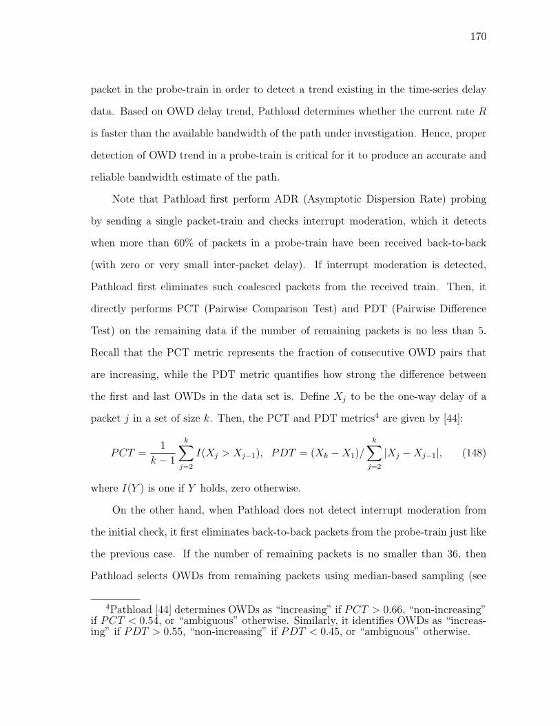
170

packet in the probe-train in order to detect a trend existing in the time-series delay

data. Based on OWD delay trend, Pathload determines whether the current rate R

is faster than the available bandwidth of the path under investigation. Hence, proper

detection of OWD trend in a probe-train is critical for it to produce an accurate and

reliable bandwidth estimate of the path.

Note that Pathload first perform ADR (Asymptotic Dispersion Rate) probing

by sending a single packet-train and checks interrupt moderation, which it detects

when more than 60% of packets in a probe-train have been received back-to-back

(with zero or very small inter-packet delay). If interrupt moderation is detected,

Pathload first eliminates such coalesced packets from the received train. Then, it

directly performs PCT (Pairwise Comparison Test) and PDT (Pairwise Difference

Test) on the remaining data if the number of remaining packets is no less than 5.

Recall that the PCT metric represents the fraction of consecutive OWD pairs that

are increasing, while the PDT metric quantifies how strong the difference between

the first and last OWDs in the data set is. Define Xj to be the one-way delay of a

packet j in a set of size k. Then, the PCT and PDT metrics4 are given by [44]:

PCT =1

k − 1

k∑j=2

I(Xj > Xj−1), PDT = (Xk −X1)/k∑

j=2

|Xj −Xj−1|, (148)

where I(Y ) is one if Y holds, zero otherwise.

On the other hand, when Pathload does not detect interrupt moderation from

the initial check, it first eliminates back-to-back packets from the probe-train just like

the previous case. If the number of remaining packets is no smaller than 36, then

Pathload selects OWDs from remaining packets using median-based sampling (see

4Pathload [44] determines OWDs as “increasing” if PCT > 0.66, “non-increasing”if PCT < 0.54, or “ambiguous” otherwise. Similarly, it identifies OWDs as “increas-ing” if PDT > 0.55, “non-increasing” if PDT < 0.45, or “ambiguous” otherwise.

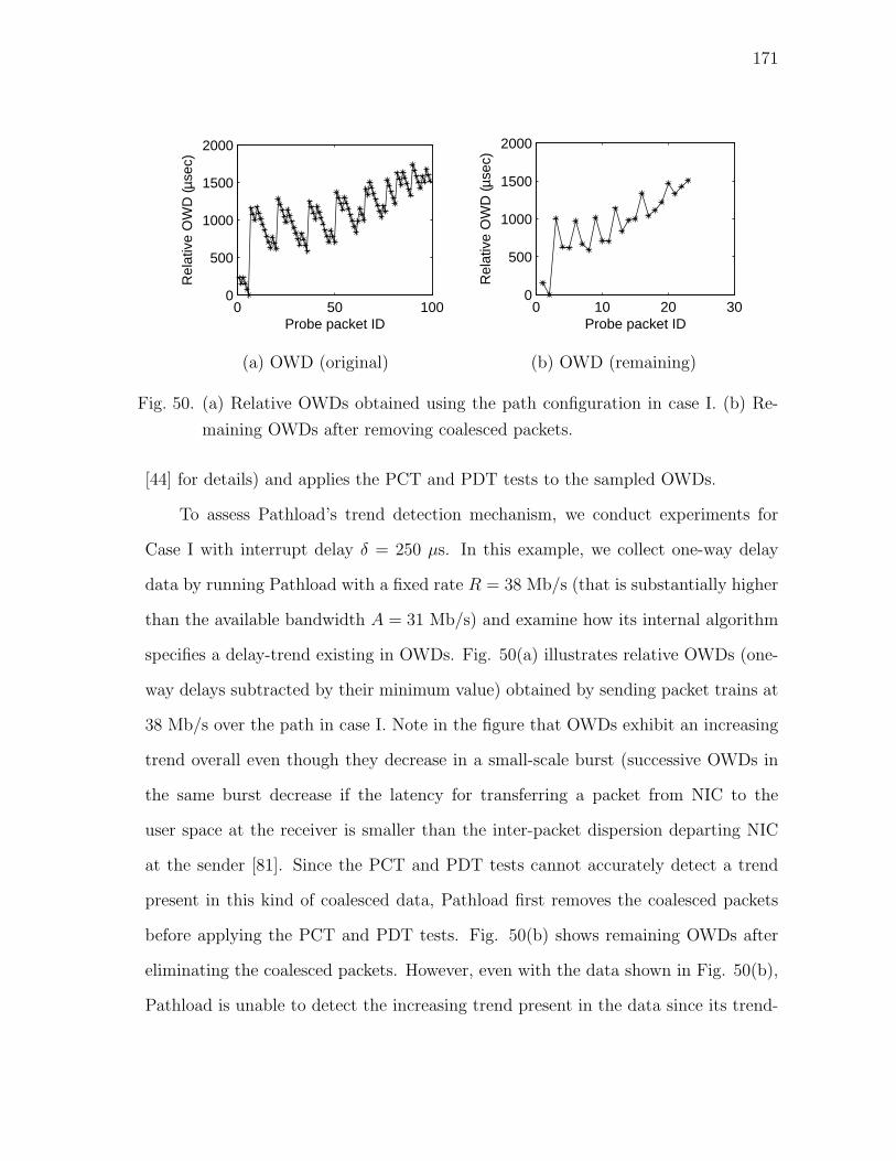
171

0 50 1000

500

1000

1500

2000

Probe packet ID

Rel

ativ

e O

WD

(µse

c)

(a) OWD (original)

0 10 20 300

500

1000

1500

2000

Probe packet ID

Rel

ativ

e O

WD

(µse

c)

(b) OWD (remaining)

Fig. 50. (a) Relative OWDs obtained using the path configuration in case I. (b) Re-

maining OWDs after removing coalesced packets.

[44] for details) and applies the PCT and PDT tests to the sampled OWDs.

To assess Pathload’s trend detection mechanism, we conduct experiments for

Case I with interrupt delay δ = 250 µs. In this example, we collect one-way delay

data by running Pathload with a fixed rate R = 38 Mb/s (that is substantially higher

than the available bandwidth A = 31 Mb/s) and examine how its internal algorithm

specifies a delay-trend existing in OWDs. Fig. 50(a) illustrates relative OWDs (one-

way delays subtracted by their minimum value) obtained by sending packet trains at

38 Mb/s over the path in case I. Note in the figure that OWDs exhibit an increasing

trend overall even though they decrease in a small-scale burst (successive OWDs in

the same burst decrease if the latency for transferring a packet from NIC to the

user space at the receiver is smaller than the inter-packet dispersion departing NIC

at the sender [81]. Since the PCT and PDT tests cannot accurately detect a trend

present in this kind of coalesced data, Pathload first removes the coalesced packets

before applying the PCT and PDT tests. Fig. 50(b) shows remaining OWDs after

eliminating the coalesced packets. However, even with the data shown in Fig. 50(b),

Pathload is unable to detect the increasing trend present in the data since its trend-

172

test produces PCT = 0.5 and PDT = 0.11, which leads to incorrect conclusion. This

indicates that Pathload’s trend-detection mechanism is not robust under the presence

of coalesced packets due to interrupt delays.

Note that Pathload often discards entire packet-trains even with strong presence

of a trend in the data due to the number of remaining OWDs after removing coalesced

packets being too small (less than 36) when interrupt moderation is not detected.

This situation happens since Pathload divides a single packet-train into subgroups

when one or more packets in a probe-train experience(s) unusually large delay (e.g.,

over 1000 µs) due to context switching or some unknown reasons in order to remove

packets affected by large sending delay in trend detection. In summary, we believe

that Pathload’s inaccuracy in trend detection is the major problem that makes it

unlikely to be successful in real networks such as the Internet.

2. IMRP: Interrupt Moderation Resilient Pathload

Motivated by the difficulty of characterizing delay variations in measured noisy OWD

data, we study noise-filtering techniques such as wavelet-based signal processing and

window-based averaging and explore their applicability in reliably identifying a trend

from the data. In what follows below, we first investigate wavelet-based signal pro-

cessing techniques that are widely used in removing noise from various data sets

obtained empirically [16]. To overcome the effect of interrupt delays on trend detec-

tion, we apply a simple multi-level discrete wavelet transform [13] to OWDs before

performing PCT- and PDT-based trend-test.

Note that in the multi-level wavelet decomposition, each stage consists of scale

and wavelet filters followed by down-sampling by a factor of 2 and separates an

input signal into two sets of coefficients: scale and wavelet coefficients. The wavelet

coefficients represent a noise component in the input signal and thus are not processed

173

further. On the other hand, the scale coefficients are applied to the two filters in

the next level as an input to further reduce noise that might still exist in the scale

coefficients from the previous stage. As a decomposition level increases, the frequency

of wavelets used in filters decreases, capturing lower frequency components present

in the original signal.

For experiments in this section, we use the family of Daubechies wavelets [18],

which are well known standard wavelets. Specifically, we use Daubechies’ length-4

wavelets, whose scale filter coefficients are given by h0 =1 +

√3

4√

2, h1 =

3 +√

3

4√

2,

h2 =3−√3

4√

2, and h3 =

1−√3

4√

2, while its wavelet filter coefficients are g0 = h3,

g1 = −h2, g2 = h1, and g3 = −h0.

Assume that a sequence s0, s1, . . . , sn−1 is an input to the j-th stage filters. Define

cAj,k and cDj,k (where k = 0, 1, . . . , n/2) to be the scale and wavelet coefficients

produced at level j, respectively. Then, cAj,k and cDj,k are given by:

cAj,k = h0s2k + h1s2k+1 + h2s2k+2 + h3s2k+3 (149)

cDj,k = g0s2k + g1s2k+1 + g2s2k+2 + g3s2k+3. (150)

Note that when k ≥ n/2 − 1, there are not enough data in the input sequence

to compute the coefficients using (149) and (150). This is known as a boundary

condition, which requires a special treatment that adds more data points to the input

sequence [95] (if this is the case, we pad the last few OWDs as needed).

To demonstrate the effect of wavelet decomposition on trend detection, we de-

compose OWDs shown in Fig. 50(a) up to level 3 and plot in Fig. 51(a) the scale co-

efficients that represent the trend component of OWD data. Applying the same PCT

and PDT tests to the scale coefficient data, we get PCT = 0.75 and PDT = 0.78,

which means that OWDs exhibit an increasing trend according to the criteria used

174

0 5 10 150

2

4

6

8

Sca

le c

oeffi

cien

ts

Coefficient ID

(a) Wavelet

0 5 10500

1000

1500

2000

Averaging window ID

Ave

rage

of r

elat

ive

OW

Ds

(b) Average

Fig. 51. Scale coefficients of wavelet decomposition and window-based averages of

one-way delays shown in Fig. 50(a).

in Pathload (recall that Pathload fails to detect this increasing trend as discussed in

Section D.1).

Next, we explore how window-based averaging improves trend detection in noisy

data. In this approach, we take the average of OWDs in a window of size k (k-

packet sliding window). Using a smaller window makes trend-detection susceptible

to a larger interrupt delay since it may not sufficiently remove noise from OWDs (we

leave optimal selection of window size as future work). For this example, we employ

k = 10 and plot in Fig. 51(b) k-packet window averages of relative OWDs shown in

Fig. 50(a), which clearly shows an increasing trend. With these averaged OWDs, we

get PCT = 0.8 and PDT = 0.74, which leads us to conclude that an increasing trend

exists in the measured data.

We incorporate the above trend-detection mechanisms into Pathload and call it

Interrupt Moderation Resilient Pathload (IMRP). We then discuss its performance

under a variety of end-host interrupt delays.

175

Table XXV. Performance of IMRP

Estimation Interrupt Evaluation scenariomethod delay δ Case-I Case-II Case-III Case-IV Case-V Case-VIIMRP 0 µs 2.46% 1.23% 3.47% 2.69% 3.71% 6.52%

(wavelet) 100 µs 6.47% 4.5% 3.02% 4.42% 5.98% 12.17%125 µs 7.21% 2.64% 3.88% 1.32% 6.1% 10.77%500 µs 5.12% 2.17% 6.78% 3.24% 7.23% 5.56%

IMRP 0 µs 2.07% 2.24% 2.1% 2.18% 9.67% 5.05%(average) 100 µs 0.19% 0.71% 11.69% 1.32% 4.19% 6.82%

125 µs 1.44% 1.82% 12.58% 1.59% 2.64% 7.89%500 µs 4.43% 4.59% 9.27% 2.55% 8.95% 6.48%

3. Performance of IMRP

We investigate estimation accuracy of IMRP under substantially different interrupt

delays δ and report its relative estimation errors eA in Table XXV. As the table shows,

IMRP produces available bandwidth estimates for all studied cases with 88 − 99%

accuracy under a wide range (0 ≤ δ ≤ 500) of interrupt delays (it is reported in [45]

that 500 µs interrupt delay is large enough to substantially reduce CPU overhead and

achieve good throughput, which is why we show interest in it). Notice in the table

that IMRP’s estimation accuracy is indifferent for various values of δ, which indicates

its robustness to variety of NIC configurations at the end-hosts. For example, even

with a very large delay δ = 500 µs, IMRP measures the paths within eA = 10% error

in all studied cases. This is substantial improvement over that of Pathload, which

can only measure paths with small interrupt delays (i.e., δ < 125 µs) as discussed in

Section D.1.

Note that IMRP is as fast as Pathload and its measurement duration in producing

estimates is virtually same as that of Pathload since numerical computation time for

wavelet decomposition of small number (N = 100) of delay samples or for their

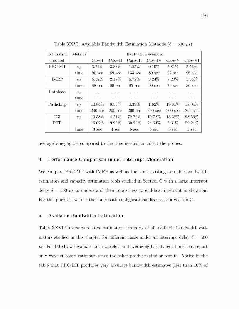
176

Table XXVI. Available Bandwidth Estimation Methods (δ = 500 µs)

Estimation Metrics Evaluation scenariomethod Case-I Case-II Case-III Case-IV Case-V Case-VI

PRC-MT eA 3.71% 3.83% 1.55% 0.19% 5.81% 5.56%time 90 sec 89 sec 133 sec 89 sec 92 sec 96 sec

IMRP eA 5.12% 2.17% 6.78% 3.24% 7.23% 5.56%time 88 sec 89 sec 95 sec 99 sec 79 sec 80 sec

Pathload eA −− −− −− −− −− −−time −− −− −− −− −− −−

Pathchirp eA 10.84% 8.53% 0.39% 1.62% 19.81% 18.04%time 200 sec 200 sec 200 sec 200 sec 200 sec 200 sec

IGI eA 10.58% 4.21% 72.76% 19.72% 13.38% 98.56%PTR 16.02% 9.93% 30.28% 24.63% 5.31% 59.24%

time 3 sec 4 sec 5 sec 6 sec 3 sec 5 sec

average is negligible compared to the time needed to collect the probes.

4. Performance Comparison under Interrupt Moderation

We compare PRC-MT with IMRP as well as the same existing available bandwidth

estimators and capacity estimation tools studied in Section C with a large interrupt

delay δ = 500 µs to understand their robustness to end-host interrupt moderation.

For this purpose, we use the same path configurations discussed in Section C.

a. Available Bandwidth Estimation

Table XXVI illustrates relative estimation errors eA of all available bandwidth esti-

mators studied in this chapter for different cases under an interrupt delay δ = 500

µs. For IMRP, we evaluate both wavelet- and averaging-based algorithms, but report

only wavelet-based estimates since the other produces similar results. Notice in the

table that PRC-MT produces very accurate bandwidth estimates (less than 10% of

177

Table XXVII. Capacity Estimation Methods (δ = 500 µs)

Methods Relative estimation error eC

Case-II Case-IVeC time eC time

PRC-MT 1.72% 89 (sec) 7.65% 86 (sec)Pathrate 17.5% 2191 (sec) 18.33% 2191 (sec)CapProbe 57.65% 500 (sec) 81.77% 500 (sec)

error) and outperforms all other existing methods studied. Even with IMRP that

uses our improved trend detection mechanisms, estimation accuracy is not as good as

PRC-MT. Observe that Pathchirp exhibits estimation accuracy that is slightly worse

than PRC-MT and IMRP in some cases (e.g., cases II, V, and VI), but comparable

to them in other cases. Note that Pathchirp’s estimation accuracy is similar to that

observed without using interrupt moderation (δ = 0) (see Table XXII), which implies

that its “jumbo” option (if selected properly) that sends substantially more packets

makes it resilient to interrupt delays. Estimation accuracy of IGI/PTR is not much

different from those cases with no interrupt delay shown in Table XXII, but is a lot

worse than that of PRC-MT and IMRP as well as Pathchirp.

b. Capacity Estimation

We compare PRC-MT with CapProbe and Pathrate in cases II and IV, in which tight

link and narrow link coincide. We show relative estimation errors eC of the above

methods in Table XXVII. As the table shows, PRC-MT produces capacity estimates

with over 90% accuracy, which significantly outperforms Pathrate and CapProbe in

the studied cases.

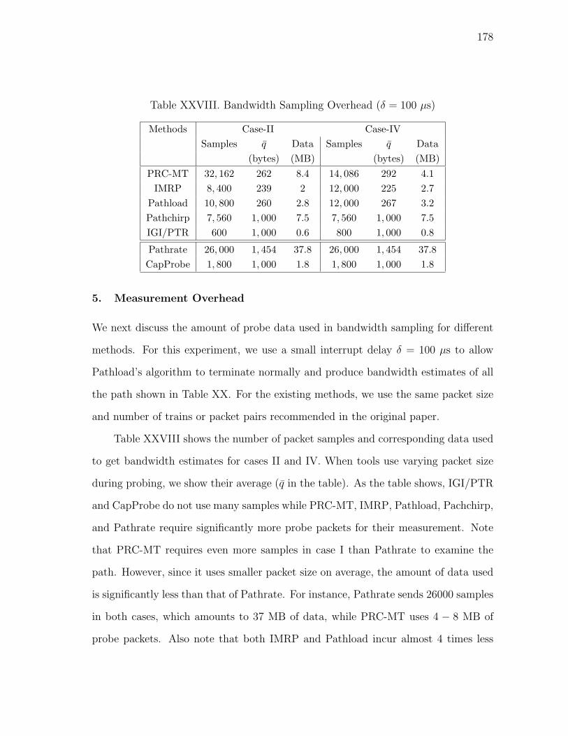
178

Table XXVIII. Bandwidth Sampling Overhead (δ = 100 µs)

Methods Case-II Case-IVSamples q Data Samples q Data

(bytes) (MB) (bytes) (MB)PRC-MT 32, 162 262 8.4 14, 086 292 4.1

IMRP 8, 400 239 2 12, 000 225 2.7Pathload 10, 800 260 2.8 12, 000 267 3.2Pathchirp 7, 560 1, 000 7.5 7, 560 1, 000 7.5IGI/PTR 600 1, 000 0.6 800 1, 000 0.8

Pathrate 26, 000 1, 454 37.8 26, 000 1, 454 37.8CapProbe 1, 800 1, 000 1.8 1, 800 1, 000 1.8

5. Measurement Overhead

We next discuss the amount of probe data used in bandwidth sampling for different

methods. For this experiment, we use a small interrupt delay δ = 100 µs to allow

Pathload’s algorithm to terminate normally and produce bandwidth estimates of all

the path shown in Table XX. For the existing methods, we use the same packet size

and number of trains or packet pairs recommended in the original paper.

Table XXVIII shows the number of packet samples and corresponding data used

to get bandwidth estimates for cases II and IV. When tools use varying packet size

during probing, we show their average (q in the table). As the table shows, IGI/PTR

and CapProbe do not use many samples while PRC-MT, IMRP, Pathload, Pachchirp,

and Pathrate require significantly more probe packets for their measurement. Note

that PRC-MT requires even more samples in case I than Pathrate to examine the

path. However, since it uses smaller packet size on average, the amount of data used

is significantly less than that of Pathrate. For instance, Pathrate sends 26000 samples

in both cases, which amounts to 37 MB of data, while PRC-MT uses 4 − 8 MB of

probe packets. Also note that both IMRP and Pathload incur almost 4 times less

179

overhead than Pathchirp.

Recall that in all experiments studied in this chapter, we use “jumbo” option to

increase Pathchirp’s estimation accuracy since without using that option, its accuracy

is significantly worse than Pathload. This result is somewhat different from that

reported in [92], which conducted simulations using ns2 with low link utilization

(at most 53%). In our experimental setup used in this work where link utilization

reaches up to 80%, Pathchirp cannot produce accurate estimates due to timestamping

inaccuracy and interrupt moderation. Higher measurement overhead of Pathchirp in

this work (different from that in [92]) accounts for the use of the jumbo option.

E. Internet Experiments

In this section, we report experimental results obtained by measuring two Internet

paths between universities in U.S. The first path is from the University of Utah

(Utah) to Texas A&M University (TAMU) and the other is from Utah to the Uni-

versity of Texas at Austin (UTexas). Note that we choose these paths simply for the

convenience of accessibility. Also note that the purpose of this experiment is not to

compare estimation accuracy of bandwidth estimators since we do not know exact

characteristics of these paths. Instead, we use this example as a sort of sanity test

for how these tools work in the Internet.

Table XXIX shows bandwidth estimates of all 8 tools investigated in this chap-

ter. In the first path, Three tools (PRC-MT, IMRP, and Pathload) produce similar

bandwidth estimates that are in a range of 86−93 Mb/s, while the others (Pathchirp

and IGI/PTR) estimate the same path as 68 Mb/s and 69 Mb/s, respectively. For

the second path (Utah-UTexas), all methods produce available bandwidth estimates

At that are in a range [79−101] Mb/s. Recall that unlike other estimators, PRC-MT

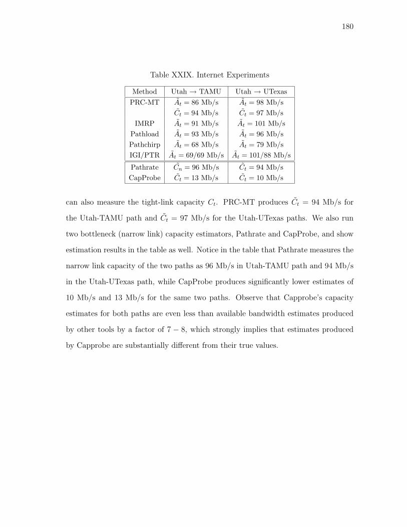
180

Table XXIX. Internet Experiments

Method Utah → TAMU Utah → UTexasPRC-MT At = 86 Mb/s At = 98 Mb/s

Ct = 94 Mb/s Ct = 97 Mb/sIMRP At = 91 Mb/s At = 101 Mb/s

Pathload At = 93 Mb/s At = 96 Mb/sPathchirp At = 68 Mb/s At = 79 Mb/sIGI/PTR At = 69/69 Mb/s At = 101/88 Mb/s

Pathrate Cn = 96 Mb/s Ct = 94 Mb/sCapProbe Ct = 13 Mb/s Ct = 10 Mb/s

can also measure the tight-link capacity Ct. PRC-MT produces Ct = 94 Mb/s for

the Utah-TAMU path and Ct = 97 Mb/s for the Utah-UTexas paths. We also run

two bottleneck (narrow link) capacity estimators, Pathrate and CapProbe, and show

estimation results in the table as well. Notice in the table that Pathrate measures the

narrow link capacity of the two paths as 96 Mb/s in Utah-TAMU path and 94 Mb/s

in the Utah-UTexas path, while CapProbe produces significantly lower estimates of

10 Mb/s and 13 Mb/s for the same two paths. Observe that Capprobe’s capacity

estimates for both paths are even less than available bandwidth estimates produced

by other tools by a factor of 7 − 8, which strongly implies that estimates produced

by Capprobe are substantially different from their true values.

181

CHAPTER VII

CONCLUSION AND FUTURE WORK

In this chapter, we summarize the major results of this thesis and discuss some future

directions for extension of this work.

A. Conclusion

In Chapter III, we studied characteristics of video streaming in best-effort networks

and proposed a preferential streaming framework called Partitioned Enhancement

Layer Streaming (PELS) that can provide a high level of end-user QoS. We further

studied modified Kelly controls in conjunction with PELS and found that they pre-

sented a good foundation for future video streaming in AQM environments. Since

the PELS framework is independent of congestion control methods employed, it can

be further used with a variety of existing and future game-theoretic or optimization-

based controllers.

In Chapter IV, we investigated the effect of random packet loss on scalable video

traffic in best-effort networks and proposed an adaptive FEC overhead control mech-

anism that can provide high quality of video to end-users. We also investigated the

characteristics of packet loss in an FEC block and derived practical models for the

distribution of the number of lost packets in a block of fixed size under Markov packet

loss. Furthermore, we examined several stochastic loss models for streaming video

and conclusively established that proper control of FEC overhead can significantly

improve the utility of received video over lossy channels.

In Chapter V, we examined the problem of estimating the capacity and available

182

bandwidth of a single congested link and showed a simple stochastic analysis of the

problem. Unlike previous approaches, our estimation did not rely on empirically-

driven methods, but instead used a queuing model of the bottleneck router that

specifically assumed non-negligible, non-fluid cross-traffic. It is also the first model

to provide simultaneous asymptotically-accurate estimation of both C and A in the

presence of arbitrary cross-traffic.

After successfully characterizing a single-congested path, we focused on measur-

ing the tight-link of a multi-hop path and developed an automated measurement tool

(called Envelope) that is based on a recursive extension of the single-hop estimator.

Through simulations, we showed that Envelope is asymptotically accurate (to the ex-

tent possible to observe using finite-sampling) in estimating both types of bandwidth.

We also presented extensive simulation results of existing methods Pathload, Spruce,

IGI, Pathrate, and CapProbe and their comparison to Envelope. These results sug-

gested that in multi-link paths with significant cross-traffic interference at non-tight

links, most existing methods cannot converge to the correct values of the bottleneck

capacity C or available bandwidth A, even if the sampling process is sufficiently long.

We further demonstrated that in many network settings, Envelope can also estimate

bandwidth for some non-tight links in the path.

In Chapter VI, we implemented a new bandwidth measurement tool called PRC-

MT that can extract both bandwidth metrics of the tight link over multi-hop paths

under arbitrary cross-traffic and routing patterns. We evaluated PRC-MT in Emulab

and PlanetLab and showed that PRC-MT produces available bandwidth and capacity

estimates with very high accuracy. We also evaluated existing bandwidth estimation

tools under various network settings and found that certain proposed algorithms

(such as Pathload) becomes susceptible to timing irregularities caused by network

hardware interrupt moderation. We identified its estimation instability under non-

183

negligible interrupt delays and found that Pathload’s instability stems from that its

delay-trend detection mechanism is unreliable when probing packets are coalesced

at the receiver. We overcame this problem using robust trend detection algorithms

(called IMRP) based on signal de-noising and showed that IMRP greatly improves

measurement stability of Pathload under various network settings.

B. Future Work

It is likely that multimedia content will be pervasive in the future Internet and the

demand for high-quality streaming services will remain very high. In order to solve

the problems related to large-scale delivery of multimedia content over the Internet,

we would like to expand this work to cover overlay networks (such as content dis-

tribution networks and peer-to-peer systems) that are increasingly used as a vehicle

to deploy new services over the current Internet without support from the underly-

ing infrastructure. This involves addressing issues associated with efficient overlay

self-reconfiguration and maintenance, load balancing among servers in the network,

and optimal selection of servers or paths for streaming services. We also have inter-

est in studying performance issues of real-time streaming in wireless environments

as increasing number of users rely on various wireless networks to gain access to the

Internet.

In addition, we have further interest in bandwidth characterization techniques,

which can directly benefit real-time streaming services over the Internet. As the

speed of network connections increases, measuring bandwidth of Internet paths can

become very susceptible to operating system (OS) and hardware-related timing irreg-

ularities because they introduce artificial delays that are unrelated to network events

such as queuing. Even though our work succeeded at designing accurate bandwidth

184

measurement techniques under the influence of timing irregularities related to net-

work hardware interrupt moderation at the receiving host, its performance in the

presence of severe OS scheduling delay jitter that depends on the CPU utilization

of the sending and/or receiving hosts requires future work. We also have interest in

further reducing measurement duration and overhead without sacrificing estimation

accuracy.

185

REFERENCES

[1] B. Ahlgren, M. Bjorkman, and B. Melander, “Network Probing Using Packet

Trains,” Swedish Institute, Tech. Rep., Mar. 1999.

[2] M. Allman and V. Paxson, “On Estimating End-to-End Network Path Proper-

ties,” in Proc. ACM SIGCOMM, Aug. 1999, pp. 263–274.

[3] E. Altman, C. Barakat, and V. M. Ramos, “Queueing Analysis of Simple FEC

Schemes for IP Telephony,” in Proc. IEEE INFOCOM, Apr. 2001, pp. 796–804.

[4] F. Baccelli, S. Machiraju, D. Veitch, and J. Bolot, “The Role of PASTA in

Network Measurement,” in Proc. ACM SIGCOMM, Sep. 2006, pp. 231–242.

[5] S. Bajaj, L. Brelau, and S. Shenker, “Uniform versus Priority Dropping for

Layered Video,” in Proc. ACM SIGCOMM, Sep. 1998, pp. 131–143.

[6] D. Bansal and H. Balakrishnan, “Binomial Congestion Control Algorithms,” in

Proc. IEEE INFOCOM, Apr. 2001, pp. 631–640.

[7] E. Biersack, “Performance Evaluation of Forward Error Correction in ATM

Networks,” in Proc. ACM SIGCOMM, Oct. 1992, pp. 248–257.

[8] P. Billingsley, Probability and Measure, 3rd ed. John Wiley & Sons, Inc., 1995.

[9] S. Blake, D. Black, M. Carlson, E. Davies, Z. Wang, and W. Weiss, “An Archi-

tecture for Differentiated Services,” IETF RFC 2475, Dec. 1998.

[10] J. Bolot, “End-to-End Packet Delay and Loss Behavior in the Internet,” in

Proc. ACM SIGCOMM, Sep. 1993, pp. 289–298.

186

[11] J. Bolot, S. Fosse-Parisis, and D. Towsley, “Adaptive FEC-Based Error Control

for Internet Telephony,” in Proc. IEEE INFOCOM, Mar. 1999, pp. 1453–1460.

[12] R. Braden, D. Clark, and S. Shenker, “Integrated Services in the Internet Ar-

chitecture: An Overview,” IETF RFC 1633, Jun. 1994.

[13] C. Burrus, R. Gopinath, and H. Guo, Introduction to Wavelets and Wavelet

Transforms: A Primer. Prentice-Hall, 1998.

[14] R. L. Carter and M. E. Crovella, “Measuring Bottleneck Link Speed in Packet

Switched Networks,” Performance Evaluation, vol. 27–28, pp. 297–318, Oct.

1996.

[15] D. Clark and W. Fang, “Explicit Allocation of Best Effort Packet Delivery

Service,” IEEE/ACM Trans. Netw., vol. 6, no. 4, pp. 362–373, Aug. 1998.

[16] P. Craigmile, P. Guttorp, and D. Percival, “Trend Assessment in a Long Mem-

ory Dependence Model Using the Discrete Wavelet Transform,” Environmetrics,

vol. 15, no. 4, pp. 313–335, May 2004.

[17] M. Dai and D. Loguinov, “Analysis of Rate-Distortion Functions and Conges-

tion Control in Scalable Internet Video Streaming,” in Proc. ACM NOSSDAV,

Jun. 2003, pp. 60–69.

[18] I. Daubechies, “Orthonormal Bases of Compactly Supported Wavelets,” Com-

munications on Pure and Applied Mathematics, vol. 41, no. 7, pp. 909–996, Oct.

1988.

[19] A. Demers, S. Keshav, and S. Shenker, “Analysis and Simulation of a Fair

Queuing Algorithm,” in Proc. ACM SIGCOMM, Sep. 1989, pp. 1–12.

187

[20] A. Dhamdhere, H. Jiang, and C. Dovrolis, “Buffer Sizing for Congested Internet

Links,” in Proc. IEEE INFOCOM, Mar. 2005, pp. 1072–1083.

[21] C. Dovrolis, P. Ramanathan, and D. Moore, “Packet-Dispersion Techniques and

a Capacity-Estimation Methodology,” IEEE/ACM Trans. Netw., vol. 12, no. 6,

pp. 963–977, Dec. 2004.

[22] C. Dovrolis, P. Ramanathan, and D. Moore, “What Do Packet Dispersion Tech-

niques Measure?” in Proc. IEEE INFOCOM, Apr. 2001, pp. 905–914.

[23] A. B. Downey, “Using PATHCHAR to Estimate Internet Link Characteristics,”

in Proc. ACM SIGCOMM, Aug. 1999, pp. 241–250.

[24] Emulab. [Online]. Available: http://www.emulab.net/. Accessed: Apr. 2008.

[25] V. Firoiu and M. Borden, “A Study of Active Queue Management for Conges-

tion Control,” in Proc. IEEE INFOCOM, Mar. 2000, pp. 1435–1444.

[26] V. Firoiu, X. Zhang, and Y. Guo, “Best Effort Differentiated Services: Trade-

off Service Differentiation for Elastic Applications,” in Proc. IEEE ICT, Jun.

2001.

[27] S. Floyd, “TCP and Explicit Congestion Notification,” ACM Comput. Com-

mun. Rev., vol. 24, no. 5, pp. 10–23, Oct. 1994.

[28] S. Floyd, M. Handley, J. Padhye, and J. Widmer, “Equation-Based Congestion

Control for Unicast Applications,” in Proc. ACM SIGCOMM, Aug. 2000, pp.

43–56.

[29] S. Floyd and V. Jacobson, “Random Early Detection Gateways for Congestion

Avoidance,” IEEE/ACM Trans. Netw., vol. 1, no. 4, pp. 397–413, Aug. 1993.

188

[30] C. Fraleigh, S. Moon, B. Lyles, C. Cotton, M. Khan, D. Moll, R. Rockell,

T. Seely, and C. Diot, “Packet-Level Traffic Measurements from the Sprint IP

Backbone,” IEEE Network, vol. 17, no. 6, pp. 6–16, Nov./Dec. 2003.

[31] P. Frossard and O. Verscheure, “Joint Source/FEC Rate Selection for Qualtiy-

Optimal MPEG-2 Video Delivery,” IEEE Trans. Image Processing, vol. 10,

no. 12, pp. 1815–1825, Dec. 2001.

[32] E. N. Gilbert, “Capacity of a Burst-Noise Channel,” Bell Systems Technical

Journal, vol. 39, pp. 1253–1265, Sep. 1960.

[33] E. Gurses, G. B. Akar, and N. Akar, “Impact of Scalability in Video Trans-

mission in Promotion-Capable Differentiated Service Networks,” in Proc. IEEE

ICIP, Sep. 2002, pp. 753–756.

[34] P. Haga, K. Diriczi, G. Vattay, and I. Csabai, “Granular Model of Packet Pair

Separation in Poissonian Traffic,” Computer Networks, vol. 51, no. 3, pp. 683–

698, Feb. 2007.

[35] K. Harfoush, A. Bestavros, and J. Byers, “Measuring Bottleneck Bandwidth of

Targeted Path Segments,” in Proc. IEEE INFOCOM, Apr. 2003, pp. 2079–2089.

[36] N. Hu, L. Li, Z. Mao, and P. Steenkiste, “Locating Internet Bottlenecks: Al-

gorithms, Measurements, and Implications,” in Proc. ACM SIGCOMM, Aug.

2004, pp. 41–54.

[37] N. Hu and P. Steenkiste, “Evaluation and Characterization of Available Band-

width Probing Techniques,” IEEE J. Sel. Areas Commun., vol. 21, no. 6, pp.

879–974, Aug. 2003.

189

[38] P. Hurley, M. Kara, J. Y. L. Boudec, and P. Thiran, “ABE: Providing a Low-

Delay Service within Best Effort,” IEEE Network Magazine, vol. 15, no. 3, pp.

60–69, May 2001.

[39] Interrupt Moderation Using Intel GbE Controllers. [Online]. Available: http://

download.intel.com/design/network/applnots/ap450.pdf. Accessed: Apr. 2008.

[40] Iperf – The TCP/UDP Bandwidth Measurement Tool. [Online]. Available:

http://dast.nlanr.net/Projects/Iperf/. Accessed: Apr. 2008.

[41] V. Jacobson, “Pathchar – A Tool to Infer Characteristics of Internet Paths.”

[Online]. Available: ftp://ftp.ee.lbl.gov/pathchar/. Accessed: Apr. 2008.

[42] V. Jacobson, “Congestion Avoidance and Control,” in Proc. ACM SIGCOMM,

Aug. 1988, pp. 314–329.

[43] M. Jain and C. Dovrolis, “End-to-End Available Bandwidth: Measurement

Methodology, Dynamics, and Relation with TCP Throughput,” in Proc. ACM

SIGCOMM, Aug. 2002, pp. 295–308.

[44] M. Jain and C. Dovrolis, “Pathload: A Measurement Tool for End-to-End

Available Bandwidth,” in Proc. Passive and Active Measurement Workshop,

Mar. 2002.

[45] G. Jin and B. L. Tierney, “System Capability Effects on Algorithms for Network

Bandwidth Measurement,” in Proc. ACM IMC, Oct. 2003, pp. 27–38.

[46] R. Johari and D. K. H. Tan, “End-to-End Congestion Control for the Internet:

Delays and Stability,” IEEE/ACM Trans. Netw., vol. 9, no. 6, pp. 818–832,

Dec. 2001.

190

[47] S. Kang, X. Liu, A. Bhati, and D. Loguinov, “On Estimating Tight-Link Band-

width Characteristics over Multi-Hop Paths,” in Proc. IEEE ICDCS, Jul. 2006.

[48] S. Kang, X. Liu, M. Dai, and D. Loguinov, “Packet-Pair Bandwidth Estimation:

Stochastic Analysis of a Single Congested Node,” in Proc. IEEE ICNP, Oct.

2004, pp. 316–325.

[49] R. Kapoor, L. Chen, L. Lao, M. Gerla, and M. Sanadidi, “CapProbe: A Simple

and Accurate Capacity Estimation Technique,” in Proc. ACM SIGCOMM, Aug.

2004, pp. 67–78.

[50] D. Katabi, M. Handley, and C. Rohrs, “Congestion Control for High Bandwidth

Delay Product Networks,” in Proc. ACM SIGCOMM, Aug. 2002, pp. 89–102.

[51] F. P. Kelly, A. K. Maulloo, and D. K. H. Tan, “Rate Control for Communication

Networks: Shadow Prices, Proportional Fairness and Stability,” J. of Oper. Res.

Soc., vol. 49, no. 3, pp. 237–252, Mar. 1998.

[52] S. Keshav, “A Control-Theoretical Approach to Flow Control,” in Proc. ACM

SIGCOMM, Sep. 1991, pp. 3–15.

[53] S. Kunniyur and R. Srikant, “Analysis and Design of an Adaptive Virtual Queue

(AVQ) Algorithm for Active Queue Management,” in Proc. ACM SIGCOMM,

Aug. 2001, pp. 123–134.

[54] K. Lai and M. Baker, “Measuring Bandwidth,” in Proc. IEEE INFOCOM, Mar.

1999, pp. 235–245.

[55] K. Lai and M. Baker, “Measuring Link Bandwidths Using a Deterministic

Model of Packet Delay,” in Proc. ACM SIGCOMM, Aug. 2000, pp. 283–294.

191

[56] L. Lao, C. Dovrolis, and M. Y. Sanadidi, “The Probe Gap Model can Underesti-

mate the Available Bandwidth of Multihop Paths,” ACM SIGCOMM Comput.

Commun. Review, vol. 36, no. 5, pp. 29–34, Oct. 2006.

[57] D. Lapsley and S. Low, “Random Early Marking: An Optimization Approach

to Internet Congestion Control,” in Proc. IEEE ICON, Oct. 1999, pp. 67–74.

[58] D. Li and D. R. Cheriton, “Evaluating the Utility of FEC with Reliable Multi-

cast,” in Proc. IEEE ICNP, Oct. 1999, pp. 97–105.

[59] J.-R. Li, S. Ha, and V. Bharghavan, “HPF: A Transport Protocol for Supporting

Heterogeneous Packet Flows in the Internet,” in Proc. IEEE INFOCOM, Mar.

1999, pp. 543–550.

[60] X. Liu, K. Ravindran, B. Liu, and D. Loguinov, “Single-Hop Probing Asymp-

totics in Available Bandwidth Estimation: Sample-Path Analysis,” in Proc.

ACM IMC, Oct. 2004, pp. 300–313.

[61] X. Liu, K. Ravindran, and D. Loguinov, “Multi-Hop Probing Asymptotics in

Available Bandwidth Estimation: Stochastic Analysis,” in Proc. ACM IMC,

Oct. 2005, pp. 173–186.

[62] X. Liu, K. Ravindran, and D. Loguinov, “What Signals Do Packet-Pair Disper-

sions Carry?” in Proc. IEEE INFOCOM, Mar. 2005.

[63] X. Liu, K. Ravindran, and D. Loguinov, “Measuring Probing Response Curves

over the RON Testbed,” in Proc. Passive and Active Measurement Workshop,

Mar. 2006.

[64] D. Loguinov and H. Radha, “End-to-End Internet Video Traffic Dynamics:

Statistical Study and Analysis,” in Proc. IEEE INFOCOM, Jun. 2002, pp.

192

723–732.

[65] S. Low, “Equilibrium Bandwidth and Buffer Allocations for Elastic Traffics,”

IEEE/ACM Trans. Netw., vol. 8, no. 3, pp. 373–383, Jun. 2000.

[66] S. Low, L. Peterson, and L. Wang, “Understanding TCP Vegas: A Duality

Model,” in Proc. ACM SIGMETRICS, Jun. 2001, pp. 226–235.

[67] S. H. Low and D. E. Lapsley, “Optimization Flow Control I: Basic Algorithm

and Convergence,” IEEE/ACM Trans. Netw., vol. 7, no. 6, pp. 861–874, Dec.

1999.

[68] S. H. Low, F. Paganini, J. Wang, S. Adlakha, and J. Doyle, “Dynamics of

TCP/RED and a Scalable Control,” in Proc. IEEE INFOCOM, Jun. 2002, pp.

239–248.

[69] S. Machiraju, D. Veitch, F. Baccelli, and J. Bolot, “Adding Definition to Active

Probing,” ACM SIGCOMM Comp. Comm. Rev., vol. 37, no. 2, pp. 17–28, Apr.

2007.

[70] B. Mah, “Pchar: A Tool for Measuring Internet Path Characteristics.” [On-

line]. Available: http://www.kitchenlab.org/www/bmah/Software/pchar/. Ac-

cessed: Apr. 2008.

[71] L. Massoulie, “Stability of Distributed Congestion Control with Heterogeneous

Feedback Delays,” IEEE Trans. Automat. Contr., vol. 47, no. 6, pp. 895–902,

Jun. 2002.

[72] B. Melander, M. Bjorkman, and P. Gunningberg, “A New End-to-End Probing

and Analysis Method for Estimating Bandwidth Bottlenecks,” in Proc. IEEE

GLOBECOM, Nov. 2000, pp. 415–420.

193

[73] Network Simulator. [Online]. Available: http://www.isi.edu/nsnam/ns/. Ac-

cessed: Apr. 2008.

[74] A. Papoulis, Probability, Random Variables, and Stochastic Processes, 2nd ed.

McGraw-Hill, 1984.

[75] K.-J. Park, H. Lim, and C.-H. Choi, “Stochastic Analysis of Packet-Pair Probing

for Network Bandwidth Estimation,” Computer Networks, vol. 50, no. 12, pp.

1901–1915, Aug. 2006.

[76] A. Pasztor and D. Veitch, “Active Probing Using Packet Quartets,” in Proc.

ACM IMW, Nov. 2002, pp. 293–305.

[77] A. Pasztor and D. Veitch, “The Packet Size Dependence of Packet Pair Like

Methods,” in Proc. IEEE/IFIP IWQoS, May 2002, pp. 204–213.

[78] V. Paxson, “Measurements and Analysis of End-to-End Internet Dynamics,”

Ph.D. Dissertation, Computer Science Department, University of California at

Berkeley, 1997.

[79] C. Perkins, O. Hodson, and V. Hardman, “A Survey of Packet Loss Recovery

Techniques for Streaming Audio,” IEEE Network, vol. 12, pp. 40–48, Sep. 1998.

[80] PlanetLab. [Online]. Available: http://planet-lab.org/. Accessed: Apr. 2008.

[81] R. Prasad, M. Jain, and C. Dovrolis, “Effects of Interrupt Coalescence on Net-

work Measurements,” in Proc. Passive and Active Measurement Workshop, Apr.

2004.

[82] QBone Scavenger Service. [Online]. Available: http://qbone.internet2.edu/

qbss. Accessed: Apr. 2008.

194

[83] H. Radha, M. Schaar, and Y. Chen, “The MPEG-4 Fine-Grained Scalable Video

Coding Method for Multimedia Streaming Over IP,” IEEE Trans. Multimedia,

vol. 3, no. 1, pp. 53–68, Mar. 2001.

[84] S. Ratnasamy and S. McCanne, “Inference of Multicast Routing Trees and

Bottleneck Bandwidths Using End-to-End Measurements,” in Proc. IEEE IN-

FOCOM, Mar. 1999, pp. 353–360.

[85] V. Ribeiro, R. Riedi, R. Baraniuk, J. Navratil, and L. Cottrell, “pathChirp:

Efficient Available Bandwidth Estimation for Network Paths,” in Proc. Passive

and Active Measurement Workshop, Apr. 2003.

[86] P. I. Richards, Manual of Mathematical Physics. Pergamon, 1959.

[87] O. Rose, “Statistical Properties of MPEG Video Traffic and Their Impact on

Traffic Modeling in ATM Systems,” in Proc. 20th Annual Conference on Local

Computer Networks, Oct. 1995.

[88] S. Shenker and L. Breslau, “Two Issues in Reservation Establishment,” in Proc.

ACM SIGCOMM, Aug. 1995, pp. 14–26.

[89] J. Shin, J. G. Kim, J. W. Kim, and C. C. Kuo, “Dynamic QoS Mapping Control

for Streaming Video in Relative Service Differentiated Networks,” European

Trans. on Telecommunications, vol. 12, no. 3, pp. 217–229, May 2001.

[90] J. Shin, J. W. Kim, and C. C. Kuo, “Quality-of-Service Mapping Mechanism

for Packet Video in Differentiated Services Network,” IEEE Trans. Multimedia,

vol. 3, no. 2, pp. 219–231, Jun. 2001.

[91] M. Shreedhar and G. Varghese, “Efficient Fair Queuing Using Deficit Round-

Robin,” IEEE/ACM Trans. Netw., vol. 4, no. 3, pp. 375–385, Jun. 1996.

195

[92] A. Shriram and J. Kaur, “Empirical Evaluation of Techniques for Measuring

Available Bandwidth,” in Proc. IEEE INFOCOM, May 2007.

[93] D. Sisalem and H. Schulzrinne, “The Loss-Delay Based Adjustment Algorithm:

A TCP-friendly Adaptation Scheme,” in Proc. ACM NOSSDAV, Jul. 1998.

[94] C. Stein, “A Bound for the Error in the Normal Approximation to the Distri-

bution of a Sum of Dependent Random Variables,” 6th Berkeley Symp. Math.

Statist. Probab., vol. 2, pp. 583–602, 1972.

[95] G. Strang and T. Nguyen, Wavelets and Filter Banks. Wellesley-Cambridge

Press, 1996.

[96] J. Strauss, D. Katabi, and F. Kaashoek, “A Measurement Study of Available

Bandwidth Estimation Tools,” in Proc. ACM IMC, Oct. 2003, pp. 39–44.

[97] Suyono and J. Weide, “A Method for Computing Total Downtime Distributions

in Repairable Systems,” Journal of Applied Probability, vol. 40, no. 3, pp. 643–

653, 2003.

[98] J. Tang, G. Morabito, I. Akyildiz, and M. Johnson, “RCS: A Rate Control

Scheme for Real-time Traffic in Networks with High Bandwidh Delay Products

and High Bit Error Rates,” in Proc. IEEE INFOCOM, Apr. 2001, pp. 114–122.

[99] K. Thompson, G. Miller, and R. Wilder, “Wide-Area Internet Traffic Patterns

and Characteristics,” IEEE Network, vol. 11, no. 6, pp. 10–23, Nov./Dec. 1997.

[100] M. van der Schaar and H. Radha, “Network and Device Driven Motion-

Compensated Scalable Video for Wireless Systems,” in Proc. Packet Video,

Apr. 2002.

196

[101] R. Wade, M. Kara, and P. Dew, “Study of a Transport Protocol Employing

Bottleneck Probing and Token Bucket Flow Control,” 5th IEEE Symposium on

Computers and Communications, 2000.

[102] R. W. Wolff, Stochastic Modeling and the Theory of Queues. Prentice Hall,

1989.

[103] H. Wu, M. Claypool, and R. Kinicki, “A Model for MPEG with Forward Er-

ror Correction and TCP-Friendly Bandwidth,” in Proc. ACM NOSSDAV, Jun.

2003, pp. 122–130.

[104] M. Yajnik, S. Moon, J. Kurose, and D. Towsley, “Measurement and Modelling

of the Temporal Dependence in Packet Loss,” in Proc. IEEE INFOCOM, Mar.

1999, pp. 345–352.

[105] H. Yousefizadeh and H. Jafarkhani, “Statistical Guarantee of QoS in Commu-

nication Networks with Temporally Correlated Loss,” in Proc. IEEE GLOBE-

COM, Dec. 2003, pp. 4039–4043.

[106] L. Zhang, S. Deering, D. Estrin, S. Shenker, and D. Zappala, “RSVP: A New

Resource Reservation Protocol,” IEEE Network, vol. 7, no. 5, pp. 8–18, Sep.

1993.

[107] Y. Zhang, S.-R. Kang, and D. Loguinov, “Delayed Stability and Performance

of Distributed Congestion Control,” in Proc. ACM SIGCOMM, Aug. 2004, pp.

307–318.

[108] L. Zhao, J. W. Kim, and C. C. Kuo, “MPEG-4 FGS Video Streaming with

Constant-Quality Rate Control and Differentiated Forwarding,” in Proc. SPIE

VCIP, Jan. 2002, pp. 230–241.

197

VITA

Seong-Ryong Kang received his B.S. degree in Electrical Engineering from Kyung-

pook National University, Korea, in 1993 and M.S. degree in Electrical Engineering

from Texas A&M University, College Station, TX, in 2000. He graduated with the

Ph.D. in Computer Science at Texas A&M University May 2008.

During 1993-1998, he worked as a patent engineer/consultant for First Intellec-

tual Property Services of Korea. His research interests include Internet video stream-

ing, network QoS and rate control, bandwidth estimation, and performance modeling

and analysis. He may be contacted at:

Seong-Ryong Kang

2500 Central Park Lane #502

College Station, Texas 77840

U.S.A.

PERFORMANCE ANALYSIS AND NETWORK PATH CHARACTERIZATION FOR

Documents

Transcript of PERFORMANCE ANALYSIS AND NETWORK PATH CHARACTERIZATION FOR