Perceptual quality improvement and assessment for virtual ...

This document is downloaded from DR‑NTU (https://dr.ntu.edu.sg)Nanyang Technological University, Singapore.

Perceptual quality improvement and assessmentfor virtual bass system

Mu, Hao

2015

Mu, H. (2015). Perceptual quality improvement and assessment for virtual bass system.Doctoral thesis, Nanyang Technological University, Singapore.

https://hdl.handle.net/10356/65644

https://doi.org/10.32657/10356/65644

Downloaded on 19 Nov 2021 21:13:29 SGT

PERCEPTUAL QUALITY

IMPROVEMENT AND

ASSESSMENT FOR VIRTUAL BASS

SYSTEM

MU, HAO

School of Electrical & Electronic Engineering

A thesis submitted to the Nanyang Technological University

in partial fulfillment of the requirement for the degree of

Doctor of Philosophy

2015

I

Acknowledgements

First and foremost, I would like to express my sincere gratitude to my

supervisor Prof. Gan Woon-Seng for his continuous guidance and support

of my PhD study. His guidance helped me in research over the past four

years and inspired me to discover further research development.

In addition, I would like to thank my senior apprentice Dr. Shi

Chuang and Dr. Tan Ee-Leng Joseph, for their generous sharing of

experience and knowledge in research and academic writing. I am also

grateful to Mr. Yeo Sung Kheng for his friendly logistical and

administrative support.

Next, I thank my lab-mates in NTU DSP Lab, past and present, Mr.

Ji Wei, Mr. Wang Tongwei, Mr. Reuben Johannes, Mr. Abhishek Seth,

Mr. Kushal Anand, Mr. Kumar Dileep, Dr. Nay Oo, Mr. Ong Say Cheng,

Mr. He Jianjun, Mr. Kaushik Sunder, Mr. Rishabh Ranjan, Mrs. Anusha

James, Mr. Chen Ciu-Hao, Mr. Phyo Ko Ko, Miss Santi Peksi, Mr.

Apoorv Agha, Mr. Lam Bhan, Mr. Cao Yi, Mr. Zou Binbin, Mr. Ang Yi

Yang and Mr. Nguyen Duy Hai. They have made the lab a warm and

interesting place to research and work.

My sincere thank also goes to all my friends in Singapore, Mr. Wang

Niyou, Dr. Luo Wuqiong, Mr. Ku Sida, Miss Yang Sha, Dr. Miao Zhenwei,

Dr. Chen Changsheng, Dr. Li Sheng, Dr. Liu Siyuan, Dr. Fan Jiayuan, Dr.

Chen Tao, Dr. Lai Jian, Miss Wang Yan, Miss Zhan Huijing, Dr. Lei

Baiying, Dr. Qin Huafeng, Mr. Li Haoliang, Miss Weng Ting, Miss Tang

Huan, Dr. Tang Peng, Mr. Tang Jianhua, Dr. Che Yueling, Dr. Leng Mei,

Dr. Hua Guang, Dr. Liao Le, Mr. Wu Kai, Mr. Li Renshi, Dr. Liu Benxu,

Mrs. Li Ya, Miss Li Peiyin, Dr. Wu Qiong, Mr. Hao Yue, Dr. Lin Han, Dr.

II

Mi Siya, Dr. Zhang Yu, Dr. Yu Xinjia, Dr. Liu Yuan, Mr. Li Qilin, Miss

Guo Yuxi, and Mr. Zhou Weigui Jair. Together with them, I had happy

and interesting life in the past four years.

Last but not least, I would also like to extend special thanks to

my parents for their understanding and support throughout my life.

III

Table of Contents

1.1 Research Area and Motivation.................................................................. 1

1.2 Major Contributions of the Thesis ............................................................ 3

1.3 Organization of the Thesis ........................................................................ 5

2.1 Missing Fundamental Effect ..................................................................... 8

2.2 Limitation of Small loudspeakers ............................................................ 10

2.3 Application of the VBS on Small Loudspeakers...................................... 13

2.4 Two Categories of the VBS..................................................................... 15

2.5 Chapter Summary................................................................................... 18

3.1 Implementation of the NLD in the VBS ................................................. 19

3.2 Implementation of the PV in the VBS.................................................... 24

3.3 Hybrid Virtual Bass System.................................................................... 32

3.3.1 Earlier Studies on Hybrid VBS ........................................................ 32

3.3.2 New Hybrid VBS.............................................................................. 34

3.4 Objective Evaluation of the Hybrid VBS................................................ 37

3.5 Chapter Summary................................................................................... 41

4.1 Improved Harmonic Synthesis in the PV................................................ 42

4.2 Harmonic Weighting Schemes................................................................. 49

IV

4.2.1 Loudness Matching Scheme.............................................................. 49

4.2.2 Fixed Weighting scheme .................................................................. 51

4.2.3 Timbre Matching Scheme ................................................................ 51

4.2.4 Objective Test and Analysis............................................................. 57

4.3 Chapter Summary................................................................................... 60

5.1 Overflow Problem in the VBS ................................................................ 61

5.2 Overflow Control using the Limiter ........................................................ 63

5.3 Automatic Gain Control Method............................................................ 66

5.3.1 Detection of Percussive Events ........................................................ 68

5.3.2 Computation of Gain Limit.............................................................. 72

5.3.3 Implementation Efficiency................................................................ 73

5.4 Comparison between Automatic Gain Control and the Limiter ............. 74

5.5 Chapter Summary................................................................................... 78

6.1 Audio Quality Evaluation ....................................................................... 80

6.2. Subjective Evaluation for the VBS ........................................................ 82

6.2.1 Playback Devices in the Subjective Test.......................................... 82

6.2.2 Subjective Test for Different VBS Techniques................................. 95

6.3 Objective Quality Assessment for the VBS............................................. 99

6.3.1 Objective Evaluation using Conventional Metrics ......................... 100

6.3.2 Proposed Perceptual Quality Metrics ........................................... 104

6.4 Analysis of Quality Metrics ................................................................. 110

6.5 Chapter Summary................................................................................. 118

7.1 Conclusions ........................................................................................... 120

7.2 Future works......................................................................................... 123

V

Summary

This research aims to develop a high-fidelity psychoacoustic bass

enhancement system for small loudspeakers in consumer audio-enabled

devices, such as laptops and flat TVs. Due to physical size and frequency

response constraints of miniaturized and flat panel loudspeakers, low-

frequency reproduction from these loudspeakers is generally limited, and

excessive amplifying low-frequency components can potentially overload

or damage loudspeakers. The proposed psychoacoustic bass enhancement

system, known as the virtual bass system (VBS), enhances the bass

perception of small loudspeakers by tricking our human auditory system

into perceiving the bass that does not exist physically. The VBS is based

on the psychoacoustic phenomenon called missing fundamental effect,

which states that higher harmonics of the fundamental frequency can

produce the sensation of the fundamental frequency in the human

auditory system. However, additional harmonics generated by the VBS

might result in perceivable distortion and reduce the perceptual quality of

VBS-enhanced signals. Hence, this thesis focuses on improving the

perceptual quality of the VBS using different techniques.

The harmonic generator is the kernel of the VBS. Earlier research

generally uses the nonlinear device (NLD) or the phase vocoder (PV) to

generate harmonic series. However, both approaches have their limitations,

and each approach is more suitable for a particular type of signals. This

thesis proposes a hybrid VBS that combines these two approaches by

analyzing the characteristic of the input signal.

Additional harmonics should be suitably weighted before mixing with

VI

the original signal, otherwise the VBS-enhanced signal may lead to

unnatural sharpness effect and heavily reduce the perceptual quality. This

thesis proposes a timbre matching scheme that adjusts the levels of

harmonic series to produce similar timbre as the original signal. Compared

to the previously used weighting scheme based on the equal-loudness

contour, the timbre matching method produces more natural sound with

reduced sharpness effect.

In addition, clipping distortion may occur in the VBS due to

arithmetic overflow during the mixing of additional harmonics and the

original signal. So far, little work has been carried out to automatically

handle arithmetic overflow in the VBS. Hence, this thesis investigates a

method to automatically control the gain settings for additional harmonics.

This method pre-computes the gain limit for additional harmonics by

analyzing high amplitude level components of the input signal. Compared

to the commonly used limiter method, the gain control method does not

require users to manually adjust the parameters (e.g. threshold and

attack/release time) for different types of audio tracks, and has no

influence on high-frequency components of the original signal.

In the design of the VBS, it is important to use an accurate way to

assess the perceptual quality across different processing methods. Earlier

research mostly carried out subjective tests, which are often time-

consuming and may be inconsistent. Therefore, it is desirable to develop

an objective quality assessment method for the VBS. Previous work on

quality assessment of the VBS only utilized some simple objective metrics,

which generally do not consider the human auditory model and are unable

to accurately predict the perceptual quality of the VBS. This thesis

introduces a perceptual quality-assessment method for the VBS based on

VII

the model output variables (MOVs) of the ITU Recommendation ITU-R

BS.1387. Our test results reveal that the derived perceptual quality

metrics have high predictive accuracy for VBS-enhanced signals.

In summary, three techniques of improving the audio quality of the

VBS and an objective metric that provides a convenient approach to

assess the perceptual quality of VBS-enhanced signals are investigated in

this thesis. Objective and subjective tests are addressed to justify the

improvement of the proposed techniques compared to previous VBS

techniques.

VIII

List of Figures

Figure 1.1 Bass enhancement using (a) the direct amplification

method and (b) the VBS.

2

Figure 1.2 Links of thesis chapters. 7

Figure 2.1 Missing fundamental effect. 9

Figure 2.2 Equal loudness contours depicting the variation in

loudness with frequency.

12

Figure 2.3 General framework of the VBS. 14

Figure 2.4 An example of bass enhancement using the direct

amplification method.

15

Figure 2.5 (a) Energy shifting of the low-frequency application.

(b) Energy shifting of the VBS.

16

Figure 2.6 Input and output plots of half-wave rectifier with a

100 Hz single tone input.

17

Figure 2.7 General framework of the NLD-based VBS 17

Figure 2.8 General framework of the PV-based VBS. 18

Figure 3.1 Input-output plot of half-wave rectifier and its

corresponding six-order polynomial expansion.

20

Figure 3.2 Magnitude response of the polynomial expansion of

half-wave rectifier NLD with a 100 Hz single tone

input.

21

Figure 3.3 Spectra of input and output signals of the polynomial

expansion of the HWR+FEXP1 NLD.

22

Figure 3.4 Input-outputs plot of the HWR+FEXP1 NLD. 22

Figure 3.5 Synthesized harmonics of a percussive signal using

the polynomial expansion of the HWR+FEXP1 NLD.

24

IX

Figure 3.6 Spectra of synthesized harmonics generated by the

HWR+FEXP1 NLD for a 100 Hz single tone input

with different peak amplitudes.

24

Figure 3.7 Two successive windowed frames along the time axis

in STFT.

26

Figure 3.8 Circular shift is applied on the windowed frame. 26

Figure 3.9 Phase spectrum of an impulse signal. 27

Figure 3.10 The sinusoid located in frequency bins of the PV. 28

Figure 3.11 Principle argument (PA) function. 29

Figure 3.12 Linear interpolation of the synthesized amplitude

𝐴𝑘𝑠(𝑛) and phase 𝜙𝑘

𝑠(𝑛) between successive frames.

31

Figure 3.13 General framework of Hill’s hybrid VBS. 33

Figure 3.14 Example of TCD weighting functions. 34

Figure 3.15 Framework of the proposed hybrid VBS. 35

Figure 3.16 The spectrum of a musical signal with percussive and

steady-state components.

36

Figure 3.17 Framework of the percussive and steady-state

separation using the proposed method.

36

Figure 3.18 Spectrograms of the separated (a) percussive and (b)


37

Figure 3.19 Separation steady-state and percussive signals using

Hill’s method.

38

Figure 3.20 Comparison between Hill’s and the proposed

separation methods for steady-state and percussive

components.

40

Figure 4.1 Pitch-shifting by two for a 250 Hz sinusoid using the

PV with a sinusoidal oscillator.

43

X

Figure 4.2 Use the proposed PV to shift the spectrum by two. 45

Figure 4.3 Phase spectrum of the 250 Hz sinusoid. 46

Figure 4.4 Use the PV to shift a single tone by three, with and

without phase coherence maintenance.

48

Figure 4.5 Harmonics’ magnitudes with exponential attenuation

schemes.

52

Figure 4.6 Source-filter model of harmonic sound generation. 53

Figure 4.7 Plots show the timbre matching weighting scheme. 55

Figure 4.8 Extracted spectral envelope from single instrument

stimuli.

56

Figure 4.9 Block diagram of the objective test for different

weighting schemes.

58

Figure 5.1 General framework of the VBS. 62

Figure 5.2 Clipping distortion in the playback due to the

arithmetic overflow of the signal.

62

Figure 5.3 Using the limiter in the VBS. 63

Figure 5.4 An example of static compression characteristic of

the limiter.

64

Figure 5.5 Block Diagrams of the limiter. 64

Figure 5.6 Using the limiter to prevent signal overflow in the

VBS-enhanced signal.

66

Figure 5.7 General framework of the proposed VBS with

feedback gain control.

67

Figure 5.8 Framework of the proposed VBS with automatic gain

control.

68

Figure 5.9 Steady-state and percussive separation using median

filter based method.

69

XI

Figure 5.10 Processing blocks of the proposed detection method

for percussive events.

69

Figure 5.11 Detection of percussive events using the HFC

function.

70

Figure 5.12 Histogram of length distribution of detected

percussive events.

72

Figure 5.13 Buffer moving in the detection of percussive events. 74

Figure 5.14 Reduce the buffer length in the detection of

percussive events.

75

Figure 6.1 Frequency response measurement of the AKG

K271MKII headphones using the dummy head.

84

Figure 6.2 Measured frequency response of (a) the Genelec

1030a loudspeaker and (b) the AKG K271MKII

headphones.

85

Figure 6.3 Setup of subjective test to compare headphones and

the loudspeaker for the VBS.

86

Figure 6.4 Calibration of SPL for (a) the Genelec 1030a

loudspeaker and (b) the AKG K271MKII

headphones.

86

Figure 6.5 MATLAB interface of the training phase in the

MUSHRA subjective test.

89

Figure 6.6 MATLAB interface for the evaluation phase in of the

MUSHRA subjective test of (a) audio quality (b)

bass intensity

90

Figure 6.7 Subjective evaluation results of audio quality for

different stimuli with 95% confidence interval.

93

Figure 6.8 Subjective evaluation results of bass intensity for

different stimuli with 95% confidence interval.

94

Figure 6.9 Framework of the quality metric training using the

linear regression model, and the quality prediction

using the trained model.

105

Figure 6.10 (a) Plot of the reference steady-state stimulus. (b)

Instantaneous NMRs of the VBS-enhanced stimuli

with different weighting schemes. The legend shows

113

XII

the MOV Total NMRB of the stimuli.

Figure 6.11 Plots of the testing percussive stimuli. 115

Figure 6.12 (a) Plot of the reference percussive stimulus. (b)

Instantaneous ModDiff of the VBS-enhanced stimuli

with gains for harmonics.

117

XIII

List of Tables

Table 3.1 Evaluation results of Hill’s and the proposed separation

method.

39

Table 4.1 ASC increment for different weighting schemes. 59

Table 5.1 Results of the overflow test using the limiter with

different thresholds.

76

Table 5.2 Results of the overflow test using the proposed gain

control method with different delay time.

77

Table 6.1 Testing stimuli in the subjective test that compares

headphones and the loudspeaker for the VBS.

87

Table 6.2 Processing methods of the stimuli in the subjective test

that compares headphones and the loudspeaker for the

VBS.

88

Table 6.3 Post-screening results for the MUSHRA tests. 91

Table 6.4 Pearson's linear correlation coefficient rl and spearman

rank correlation coefficient rs between headphones and

the loudspeaker on the subjective scores of testing

stimuli.

95

Table 6.5 Testing steady-state stimuli in the subjective test for

the VBS.

96

Table 6.6 Testing polyphonic stimuli in the subjective test for the

VBS.

96

Table 6.7 Subjective scores for the steady-state stimuli with 95%

confidence interval.

98

Table 6.8 Subjective scores for the polyphonic stimuli with 95%

confidence interval.

99

Table 6.9 Model output variables (MOVs) in the PEAQ Basic

Mode.

101


rank correlation coefficient rs between mean subjective

scores and HR, ASC and ODG.

103

XIV


rank correlation coefficient rs between mean subjective

scores and individual MOVs.

104

Table 6.12 Three groups of training stimuli. 107

Table 6.13 Selected combinations of the MOVs with maximum

MinCorr and minimum MaxRMSE for steady-state

stimuli.

109

Table 6.14 Selected combinations of the MOVs with Maximum

MinCorr and Minimum MaxRMSE for polyphonic

stimuli.

109

Table 6.15 Selected combinations of the MOVs with maximum

MinCorr and minimum MaxRMSE for combined

steady-state and polyphonic stimuli.

110

Table 6.16 ANOVA p-values for the MOVs from the derived

perceptual quality metrics for steady-state stimuli.

111


perceptual quality metrics for polyphonic stimuli.

111


perceptual quality metrics for combined steady-state

and polyphonic stimuli.

112

Table 6.19 Selected combinations of the MOVs with Maximum

MinCorr and Minimum MaxRMSE for percussive

stimuli.

116


perceptual quality metrics for percussive stimuli.

116

XV

List of Abbreviations and

Acronyms

ADB Average Distorted Block

ANC Active Noise Control

AR Anchor

ASC Audio Spectrum Centroid

CQT Constant-Q Transform

DRC Dynamic Range Compressor

EXA Exponential Attenuation

FFT Fast Fourier Transform

HFC High Frequency Content

HPF High-Pass Filter

HR Harmonic Richness

HRF Hidden Reference

HWR Half-Wave Rectifier

ISTFT Inverse Short-time Fourier Transform

ITU International Telecommunication Union

JND Just Noticeable Difference

LCB Lower Confidence Bound

LPF Low-Pass Filter

MaxRMSE Maximum RMSE

MFPD Maximum Filtered Probability of Detection

MinCorr Minimum Correlation Coefficient

MS Mean Score

MUSHRA MUltiple Stimuli with Hidden Reference and Anchor

NLD Nonlinear Device

NMR Noise to Mask Ratio

MOV Model Output Variables

XVI

ModDiff Modulation Difference

PA Principal Argument

PEAQ Perceptual Evaluation of Audio Quality

PP Polyphonic

RMSE Root Mean Square Error

SAR Sources to Artifacts Ratio

SDR Source to Distortion Ratio

SEI Spectral Envelope Instability

SIR Source to Interferences Ratio

SNR Signal to Noise Ratio

SPL Sound Pressure Level

SS Steady-State

STFT Short-time Fourier Transform

TCD Transient Content Detector

THD Total Harmonic Distortion

PV Phase Vocoder

UCB Upper Confidence Bound

VBS Virtual Bass System

XVII

List of Symbols

Ak(n) instantaneous amplitude of the kth frequency bin

Bandj bark-scale critical bands

ENV (f) spectral envelope

F0 fundamental frequency

f frequency

fc cut-off frequency

fk(n) instantaneous frequency of the kth frequency bin

fres frequency resolution of the spectrum

fs sampling frequency

G gain for harmonics

Gu gain set by users

Gm maximum gain for harmonics

GALim gain of the limiter’s characteristic cure

hi polynomial coefficients of the NLD

I(n) number of sinusoids in the PV

INLim input level of the limiter

Ihar synthesized harmonics number

jB index of Bark-scale band

jst index of stimuli

k frequency bin index

kp bin of the spectral peak

kt total compliance

Ltm number of time frames

Lwin windows length in STFT

Loudn(f) loudness in phon at frequency f

ModT(m,k) local modulation measure of testing stimuli

ModR(m,k) local modulation measure of reference stimuli

MP(m,k) masks for the percussive component

XVIII

MS(m,k) masks for the steady-state component

m time frame index

moffset offset frame of HFC

mas total moving mass

Nc number of frequency bands.

NFFT FFT length

Npoly order of polynomial expansion of the NLD

n sample index

noffset detected offset sample index

QDE(m) distortion steps above the threshold

OUTLim output level of the limiter

PW(m,k) signal’s power spectrum

PDE(m) probability of noise detection

Px(m,k) percussive-enhanced components

Ra analysis hop size in STFT

RASC incensement of ASC

rl linear correlation coefficient

rs Spearman rank correlation coefficient

SCASC ASC scores

Sc cone of piston area

Sx(m,k) steady-state-enhanced components

sQA predicted score using trained metrics

sHA(n) synthesized steady-state harmonics

SPL( f ) sound pressure level in dB at frequency f

TLim threshold of the limiter’s characteristic cure

TFj(k) triangular filter

Ts sampling period

u integer value

VQA matrix of MOVs

Wi weight for harmonics

wNLD weight for the NLD in the hybrid VBS

wPV weight for the PV in the hybrid VBS

XIX

wQA linear weightings for the MOVs

wQA vector of linear weightings for the MOVs

X(m,k) spectrum of the input signal

XPV(m,k) spectrum of the input signal in the PV

x(n) input signal of the VBS

xHF(n) high-frequency components of the input signal

xHA(n) synthesized higher harmonics of the VBS

xLF(n) low-frequency components of the input signal

xLim(n) input signal of the limiter

xNLD(n) input signal of the NLD

xPV(n) input signal of the PV

Y(m,k) synthesized spectrum

YPV(m,k) synthesized spectrum of the PV

y(n) output signal of the VBS

yLim(n) output signal of the limiter

yNLD(n) output signal of the NLD

ypl(n) detected peak level of the limiter

yPV(n) output signal of the PV

yQA subjective scores of testing stimuli

yQA vector of subjective scores

η power efficiency of the loudspeaker

ϕk(n) instantaneous phase of the kth frequency bin

1

Introduction

1.1 Research Area and Motivation

Driven by the ever-growing demand for smaller media devices, slimmer

notebooks and flatter TV displays, it has become very challenging to

manufacture sufficiently sized loudspeakers that are capable of producing

low-frequencies (or bass). Bass components of the audio signal, which

imbue listeners with a sense of power and contain the fundamental

frequency of the rhythm section, are generally below 250 Hz [1]. However,

due to the form-factor limitation, small loudspeakers cannot efficiently

reproduce the sound in this low-frequency range [2], leading to poor

perception of bass reproduction and lacks of strong rhythms. The

conventional method to enhance bass effect is directly amplifying the

intensity of low-frequencies, as shown in Figure 1.1(a). However, due to

the limited movement of the loudspeaker diaphragm, the direct

amplification method usually leads to distortion, and might overload or

damage loudspeakers [3].

In 1999, Shashoua et al. [4] introduced a psychoacoustic bass

enhancement system to stimulate the human sensation of bass perception,

and such techniques have been successfully deployed in some commercial

systems such as MaxxBass [5] and Ultra Bass [6]. In this thesis, we call

this system the virtual bass system (VBS). The VBS is based on a

psychoacoustic phenomenon, known as the missing fundamental effect [7],

2

[8], which states that higher harmonics of the fundamental frequency can

cause the human brain to infer the sensation of the fundamental frequency

even though it is not physically reproduced. For example, in the absence

of the fundamental frequency at 100 Hz, the human brain can be tricked

into perceiving the 100 Hz tone using the harmonic series at 200, 300, 400,

and 500 Hz (i.e., extracting the common difference frequency within the

harmonic series). In other words, a loudspeaker having a high cut-off

frequency fc above the fundamental frequency F0 can virtually produce the

sensation of F0 by injecting a series of suitably weighted harmonics,

instead of boosting the F0, as shown in Figure 1.1(b).

The VBS has been researched for more than a decade and successfully

applied in many related areas, including the virtual surround sound

system [9], crosstalk cancellation [10], active noise control (ANC) headsets

[11], parametric array loudspeakers [12], [13], flat television sets [14],

multichannel flat-panel loudspeakers [15], physically-based correction

frequency responsefrequency response

frequency responsefrequency response VBS

fc 2F0 3F0 4F0 5F0 6F0fcF0

fcF0 fcF0

(b)

(a)

Amplification

∆F= F0

Figure 1.1. Bass enhancement using (a) the direct amplification method

and (b) the VBS. (red line: frequency response of small loudspeakers)

3

technique for the problematic room-mode [16], and reduction of low-

frequency noise in discos and clubs [2].

However, additional harmonics generated by the VBS might result in

perceivable distortion and reduce the perceptual quality of VBS-enhanced

signals. There is a trade-off between the perceived bass intensity and the

audio quality of VBS-enhanced signals. Increasing the gain for harmonics

introduces more perceptual bass but also leads to higher distortion. Most

of earlier studies on the VBS focus on selecting suitable harmonic

generators [2], [17]–[21] without much consideration on other approaches.

This thesis focuses on the techniques of improving the quality of the VBS

in broader aspects.

The major objectives of this dissertation are highlighted as follows:

Design a VBS that can select a suitable harmonic generator

based on characters of the input signal.

Enhance the perceptual quality of the VBS by matching the

timbre of the VBS-enhanced signal to the original signal.

Devise an approach to handle arithmetic overflow due to

additional harmonics.

Build perceptual quality evaluation metrics to effectively grade

the performance of different VBS techniques.

1.2 Major Contributions of the Thesis

This thesis focuses on the techniques of improving the perceptual

quality of the VBS. Its major contributions are highlighted as follows:

I. Proposal of the hybrid VBS. The VBS generally uses the nonlinear

device (NLD) or the phase vocoder (PV) to generate harmonic series.

However, both generators have their strengths and weaknesses. It was

4

found that the NLD-based VBS is more suitable for the percussive

components (used here to refer to signals that concentrate their energy in

a short time period and have wideband spectra, such as the drum beats),

whereas the PV-based VBS is more applicable to steady-state signals

(used here to refer to tonal components with highly harmonic structure,

such as bass guitar). Hence, we build a hybrid VBS that combines these

two approaches to take advantages of the two harmonic generators and

achieve a more stable bass enhancement performance.

II. Proposal of a timbre matching approach for the steady-state

components in the VBS. We propose a new timbre matching technique,

which can improve the audio quality of steady-state VBS-enhanced

components in the PV. This approach adjusts the amplitude of harmonic

series to produce similar timbre to the original audio signal. The objective

test indicates that the proposed method can improve the timbre sharpness

problem of VBS-enhanced signals and produce more natural bass.

III. Proposal of an overflow control method for the VBS. The VBS

technique of adding synthesized harmonics to the original signal may lead

to arithmetic overflow and cause clipping distortion, especially during

high-level percussive components. There is little work carried out in

reducing signal overflow for the VBS, and manual gain control is required

to avoid overflow, which is very troublesome. Hence, we propose a VBS

technique that can efficiently overcome the overflow problem by

automatically controlling the gain settings for additional harmonics. The

proposed approach pre-computes the gain limitation for additional

harmonics by analyzing high amplitude level components of the input

signal, and it can be adopted for real-time implementation. Compared to

the commonly used limiter method, the proposed gain control method

5

does not require users to manually adjust the parameters for different

types of audio tracks, and does not influence high-frequency components

of the original signal.

IV. Design of an objective assessment method for the perceptual

quality of the VBS. Because subjective tests often demand lengthy setup

and time-consuming procedure, it is desirable to develop an objective

assessment method for the VBS. Earlier studies only utilized some simple

objective metrics, which generally do not consider the human auditory

model and are unable to accurately predict the perceptual quality of VBS-

enhanced signals. In this thesis, we introduce a perceptual quality

assessment method for the VBS based on the model output variables

(MOVs) of the ITU Recommendation ITU-R BS.1387. The testing result

reveals that the derived perceptual quality metrics have high predictive

accuracy for VBS-enhanced signals.

1.3 Organization of the Thesis

This thesis is organized as shown in Figure 1.2. In Chapter 2, research

on the missing fundamental effect is reviewed, and the fundamental of the

VBS is introduced. In Chapter 3, a hybrid structure VBS is proposed,

which separates inputs signals into percussive and steady-state

components, and applies NLD and PV on the separated signals. This new

hybrid structure takes advantages of the two harmonic generators and has

a more stable performance. In Chapter 4, an improved harmonic synthesis

approach and a timbre matching scheme are proposed for the PV. These

methods are applied to improve the perceptual quality of harmonics from

steady-state components. In Chapter 5, a gain control method for

harmonics is proposed to prevent overflow distortion in the VBS. Because

6

signal overflow is much more likely to occur in high level signals, the gain

control is based on the detection of percussive events that generally have

high amplitude levels. In Chapter 6, an objective assessment method for

the perceptual quality of the VBS is proposed, which is a more efficient

way compared to time-consuming subjective tests. Finally, Chapter 7

concludes this thesis and discuses some future works based on the current

contributions.

7

Figure 1.2. Links of thesis chapters.

take their advantages

Chapter 1Introduction

Chapter 2 Missing Fundamental Effect and the Virtual Bass System

Chapter 4Quality Improvement for the Phase Vocoder

Chapter 5Overflow Control in the

Virtual Bass System

Chapter 6Quality Assessment of the Virtual Bass System

Steady-state components

Percussive components

Basic Theory: Missing fundamental effect

Chapter 7Conclusions and Future Work

Comparison with amplification

Motivation: poor bass of small loudspeakers

Chapter 3Hybrid Virtual Bass System

NLD based VBSPV based VBS

Hybrid VBS

8

Missing Fundamental Effect and

the Virtual Bass System

This chapter presents the fundamental of the virtual bass system (VBS).

History of the missing fundamental effect, which is the fundamental

principle of the VBS, is reviewed in Section 2.1. In Section 2.2, the

limitation of small loudspeakers in reproducing low-frequency components

is discussed. It is found that physical modifications on the loudspeaker

design cannot effectively overcome the problem of their poor bass

performance. Hence, Section 2.3 illustrates the application of the VBS on

small loudspeakers. We find that the VBS is more effective in improving

small loudspeakers’ bass performance compared to the conventional direct

amplification method. Subsequently, Section 2.4 introduces two commonly

used types of the VBS based on the nonlinear device (NLD) and the phase

vocoder (PV). Finally, Section 2.5 summarizes the main findings in this

chapter.

2.1 Missing Fundamental Effect

Individual sine wave components, that are integer related with each

other, are called harmonics [22]. The lowest frequency is called the

fundamental frequency F0 or the first harmonic, and the higher frequency

harmonics are called the 2nd, 3rd… harmonics. The frequency of

the ……………..second harmonic is twice the frequency of F0 and so on. The

missing fundamental effect [7], [8] states that higher harmonics (2F0, 3F0,

9

4F0…) can produce the sensation of the F0 in the human auditory system,

as shown in Figure 2.1.

Scientific studies on the perception of the fundamental frequency

began in the 19th century, and it was firmly established in the mid-20th

century. In 1843, Ohm [23] proposed that the human ear can separate a

complex tone composed of harmonics F0, 2F0, 3F0… into pure harmonics,

and found that the pitch of the complex tone was derived directly from

the lowest harmonic F0. In contrary, Seebeck [24], [25] reported some

experiment results on the conditions for hearing tones, and showed that

the complex tone still produced the perception of F0 when the F0

component was almost removed. This was the first presentation of the

missing fundamental effect. However, Helmholtz [26] strongly promoted

Ohm's view and elaborated it as Ohm’s acoustic law:

"A pitch corresponding to a certain frequency can only be heard if the

acoustical wave contains power at that frequency" [22]. This law was

generally accepted for nearly a century.

In the mid-20th century, Schouten [27]–[29] carried out some

experiments to investigate the missing fundamental effect with the help of

an optical siren (an acoustical instrument for producing musical tones).

The results showed that complete elimination of F0 from the complex tone

did not alter its pitch. A more conclusive experiment was carried out by

Human auditory system

∆F=F0

F0 2F0 3F0 4F0 5F0 6F0 F0 2F0 3F0 4F0 5F0 6F0

Figure 2.1. Missing fundamental effect.

10

Licklider [30], [31]. He showed that F0 was perceived from higher

harmonics in the presence of a low-frequency noise that masks the

fundamental component. These experimental results contradicted Ohm’s

acoustic law and confirmed the perception of the missing fundamental

effect.

Subsequent studies in this area were carried out in terms of the most

important harmonics for pitch perception. The harmonics that are most

important are called the dominant harmonics, and the frequency region in

which these harmonics occupied is called the dominant region [32]. Plomp

[33] found that the pitch was determined by the 4th and higher harmonics

for F0 up to about 350 Hz; and by the 3rd and higher harmonics for F0 up

to about 700 Hz. Ritsma’s [34] concluded that the frequency band that

includes the third, fourth and fifth harmonics determines the perception of

F0 in the range of 100 to 400 Hz. Moore [35] found that for complex tones

with fundamental frequencies of 100, 200, or 400 Hz and with equal-level

harmonics, the dominant harmonics were always within the first six

harmonics. Dai [36] found that dominance region has a fixed width in

harmonic number (three or four), and harmonics closest to 600 Hz are

dominant for F0 from 100 to 800 Hz.

2.2 Limitation of Small loudspeakers

With the development of portable media devices, such as mobile

phones and tablet computers, the demand to reproduce high-quality bass

(low-frequency) effect with small loudspeakers has never been greater.

However, due to the physical size limitation and cost constraint, these

small loudspeaker units are unable to reproduce good or sufficient bass.

This bass production limitation can be explained using the following

11

loudspeaker modeling equations [2]:

2

,

1,

2

c

t

c

S

mas

kf

mas

(2.1)

where η denotes the power efficiency (ratio of acoustically radiated power

and electrical power) of the loudspeaker, Sc represents the cone of piston

area, mas represents the total moving mass, fc is the cut-off frequency,

and kt is the total compliance that combines suspension and cabinet

influence. Size of the driver and the cabinet are limited in small

loudspeakers, leading to a small cone area Sc and a high compliance kt.

Hence, a low fc requires a large mass, which greatly decreases the

efficiency η of the loudspeaker. For example, to lower the fc of an octave

by quadrupling the mas, the efficiency η need to be decreased by a factor

of 16 (12 dB). On the other hand, lowering kt is not feasible because it

requires a large cabinet volume.

Beyond the size limitation of loudspeakers, another problem comes

from the loudness for low-frequency signals. According to the equal-

loudness contour shown in Figure 2.2, it requires higher sound pressure

level (SPL) to achieve the same loudness for low-frequency signals

compared to mid-frequency signals. For example, to achieve the loudness

of 80 phon, a 1000 Hz sinusoid must produce an 80 dB SPL, whereas a

125 Hz sinusoid must produce a higher SPL of 90 dB.

Appendix A shows the measurement on frequency responses of several

small loudspeakers. It was found that most of these small loudspeakers

have a high cut-off frequency. For example, a capsule loudspeaker

(60× 44× 44 mm) with a 40 mm driver has a cut-off frequency at 447 Hz,

and the cut-off frequency of a portable outdoor loudspeaker (88× 35× 35

12

mm) with a 25.4 mm driver is as high as 562 Hz.

Design improvements of the loudspeaker system can yield better low-

frequency performance. Some portable loudspeakers have an extendable

body to enlarge its cabinet, as shown in Figure A.1 and A.2. In Appendix

A, we measured the frequency response of two capsule loudspeakers with

an extendable cabinet. After the extension, the cut-off frequency of one

loudspeaker is decreased from 398 Hz to 334 Hz, and its response roll-off

is reduced by 1 dB/octave; the response roll-off of another loudspeaker is

reduced by 3 dB/octave, but its cut-off frequency did not change. Another

technique for bass enhancement is the ported enclosure (also known as the

bass reflex), which has a vent opening in the wall of the cabinet, as shown

in Figure A.4. The vent allows air to flow through, and introduces an

additional resonance to extend the low-frequency response. The drawback

of the ported enclosure is that the response rolls off much faster below the

fc and the temporal behavior is degraded [2]. The measured ported

loudspeaker, as shown in Figure A.4, has a 19.5 dB/octave response roll-

Frequency (Hz)

Sou

nd p

ress

ure

lev

el (

dB

)

Figure 2.2. Equal loudness contours depicting the variation in loudness

with frequency. Source from [37].

13

off, whereas the response roll-off of other small loudspeakers is from 8.9 to

13.4 dB/octave. In summary, limitation of low-frequency performance in

small loudspeakers cannot be effectively overcome with simple

modifications on design of the loudspeaker system.

2.3 Application of the VBS on Small Loudspeakers

As the design techniques for the loudspeaker system cannot effectively

enhance the bass effect of small loudspeakers, signal processing techniques

for bass-enhancement are studied. There are two signal processing

techniques to enhance the bass performance: direct bass amplification

(physical method) and the VBS (psychoacoustic method).

Direct amplification is a conventional method to boost the energy of

signal’s low-frequency components. However, due to small loudspeakers’

intrinsic low efficiency in reproducing low-frequencies, the amplification

method cannot effectively enhance the bass perception [2]. In addition,

over-amplification can potentially overload or damage loudspeakers. On

the other hand, the VBS stimulates the human sensation of bass

perception by injecting harmonics in the mid-frequency range, where

majority of loudspeakers have relatively good reproduction ability. Based

on the missing fundamental effect as described in Section 2.1, listeners can

perceive virtual bass effect even though physical bass frequencies are

missing.

The general framework of the VBS is shown in Figure 2.3. Low-

frequency components xLF(n) (where n represents the discrete time sample

index) of the input signal x(n) are extracted using a low-pass filter (LPF),

and fed into the harmonic generator to synthesize higher harmonics xHA(n).

The cut-off frequency of the LPF is determined according to the cut-off

14

frequency of the loudspeaker. However, low-frequency components that

imbue listeners with a sense of power and contain the fundamental

frequency of the rhythm section are mainly in the range below 250 Hz [1].

In addition, large amount of additional high-frequency components may

increase the sharpness effect [37] in the VBS-enhanced signal. Therefore,

low-frequency components that are extracted for harmonic synthesis

should lie within the range below 250 Hz, even though the cut-off

frequency of the loudspeaker is higher than 250 Hz. Meanwhile, a high-

pass filter (HPF) is used to remove redundant low-frequency components

of the original signal that cannot be reproduced by loudspeakers. This

results in more headroom to add in synthesized harmonics.

In contrast, the direct amplification method requires attenuation of the

entire signal to create headroom for increment of the low-frequency energy.

As an example shown in Figure 2.4, the direct amplification method is

used to enhance the low-frequency comments below 150 Hz with 3 dB

gain for an audio track with 1 dB headroom. However, the amplitude level

of the bass-boosted signal overshoots the range of 0 dB, which causes

arithmetic overflow and leads to distortion in the playback. Hence, the

bass-amplified signal should be attenuated before the output. As a result,

high-frequency components of the original signal are also attenuated,

which may degrade its perceptual quality.

inputsignal

LPF +

HPF

Harmonicgenerator

output signal

F0 2F0 … 6F0

G

xHF(n)

xHA(n)

y(n)x(n)

xLF(n)

Figure 2.3. General framework of the VBS. (LPF and HPF: low-pass

and high-pass filters; G: gain for harmonics).

15

Figure 2.5 illustrates the difference between the two bass enhancement

methods in the aspect of energy shifting. The direct amplification method

shifts the energy from mid and high frequency components to boost low-

frequency components; while the VBS shifts the redundant low-frequency

energy to mid-frequency components, which can be reproduced more

efficiently by small loudspeakers.

2.4 Two Categories of the VBS

The harmonic generator plays a key role in the VBS. There are two

types of the VBS based on the harmonic generator, the nonlinear device

(NLD)-based [5], [6], [38], [2], [17]–[19], [39], [15], [40], [20], [3] and the

phase vocoder (PV)-based [21], [41], [42].

LPF

inputsignal bass-amplified

signal

+

HPF

+3dB

0 2 4 6 8-15

-10

-5

0

0 2 4 6 8-15

-10

-5

0

+Attenuation

(<0dB)

Time (sec)Time (sec)

Lev

el (

dB

)

0 2 4 6 8-15

-10

-5

0

Time (sec)

Lev

el (

dB

)

outputsignal

Figure 2.4. An example of bass enhancement using the direct

amplification method.

16

The NLD has been used in many psychoacoustic bass enhancement

systems, such as MaxxBass [5], Ultra Bass [6], and the VBS [17]–[20].

Some commonly used NLD includes multiplier, rectifier and clipper, which

are generally memory-less functions. Figure 2.6 shows the nonlinear

transfer function of the half-wave rectifier (HWR), which produces

fundamental and even order harmonics. A comprehensive review of NLDs

that are useful for the VBS can be found in [2], and Oo and Gan [20] used

subjective and objective methods to evaluate the performance of different

NLDs for the VBS.

Larsen and Aarts [2] introduced a general framework of NLD-based

VBS, as shown in Figure 2.7. The NLD-based VBS works in the time-

domain. Low-frequency components of the original signal are distorted by

the NLD to produce harmonics. The band-pass filter (BPF) shapes the

spectral envelope of synthesized harmonics to produce a more natural and

pleasant sound [2].

The PV is a well-known tool to perform time-scaling or pitch-shift for

speech and audio signals based on the short-time Fourier transform

(STFT) [43]. The PV was first introduced by Flanagan [44] in 1966, and

improved by Griffin et al. [45] and Laroche et al. [46], [47] in 1984 and

Low frequencyregion

Mid and high frequencyregion

Energy Energy

Low frequencyregion

Mid frequencyregion

(a) (b)

Figure 2.5. (a) Energy shifting of the low-frequency application. (b)

Energy shifting of the VBS.

17

1999, respectively. The PV-based VBS was first proposed by Bai et al. [21]

in 2006.

Different from the NLD-based VBS, the PV-based VBS operates in the

frequency domain. Relevant harmonics are synthesized based on the

extracted information of the input signal. The general framework of the

PV-based VBS is shown in Figure 2.8. Low-frequency components of the

input signal are transformed into frequency domain using STFT.

0 0.2 0.6 1-0.2-0.61

Input

-0.5

0

0.5

1

Outp

ut

0

10

20

30

40

50

60

70

80

90

100

Frequency(Hz)

Mag

nit

ude

(dB

)

10

20

30

40

50

60

70

80

90

100

Mag

nit

ude

(dB

)

Frequency(Hz)0 500 1000 1500

00 500 1000 1500

100Hz100Hz

200Hz

400Hz600Hz

800Hz1000Hz

1200Hz1400Hz

y=0.5(x+|x|)

Figure 2.6 with a

100 Hz single tone input

outputsignal

+GNLD

inputsignal

HPF

LPF BPF

Figure 2.7. General framework of the NLD-based VBS [2].

18

Subsequently, the instantaneous frequencies of low-frequency components

are estimated based on the phase information of the input spectrum, and

pitch-shifted signals are generated using a sinusoid oscillator.

2.5 Chapter Summary

In this chapter, the historical study of missing fundamental effect was

reviewed, and the first six harmonics were found to be the most important

harmonics for perception of F0. Subsequently, the limitation of

reproducing low-frequency components from small loudspeakers was

introduced. Because of the size constraint, design techniques of the

loudspeaker system and the conventional low-frequency amplification

method cannot effectively enhance the bass effect of small loudspeakers.

On the other hand, the proposed VBS technique is more effective, because

it stimulates the human sensation of bass perception by injecting

harmonics in mid-frequencies, which can be effectively reproduced by

small loudspeakers. In addition, it was found that the VBS was most

suitable to enhance frequency components below 250 Hz. Finally, we

introduced two common categories of VBS, the NLD-based and the PV-

based. The details of implementing NLD and PV in the VBS will be

introduced in the following chapter.

Harmonicsynthesizer

outputsignal

+LPFPitch

detectionGSTFT

Phase Vocoderinputsignal

HPF

Figure 2.8. General framework of the PV-based VBS.

19

Hybrid Virtual Bass System

The previous chapter introduces two common categories of VBS based on

different harmonic generation methods, namely the nonlinear device (NLD)

and the phase vocoder (PV). In this chapter, the theoretical development

of applying NLD and PV in the VBS are introduced in Section 3.1 and 3.2,

respectively. However, both harmonic generators have their limitations,

and individual approach is found to be more applicable to a particular

component of the input signal. Hence, in Section 3.3, we propose a hybrid

VBS that separates the input signal and sends different components into

the two harmonic generators, hence taking advantages of both NLD and

PV. The effect of the hybrid VBS is objectively evaluated in Section 3.4.

Finally, Section 3.5 summarizes the main findings in this chapter.

3.1 Implementation of the NLD in the VBS

The NLD-based VBS makes use of nonlinearity to generate harmonics,

and NLDs generally produce infinite series of harmonics. As mentioned in

Section 2.1, psychoacoustic research found that the human auditory

system is most sensitive to the second to sixth harmonics for pitch

perception [35]. In addition, a large number of higher harmonics may

distort the original components in the mid-frequency range and increase

the sharpness effect [37]. Therefore, it is only necessary to generate

harmonics up to the sixth order.

For this purpose, a polynomial expansion of a particular function is

20

used as an approximation of the memory-less NLD in the VBS [18]. The

polynomial approximated NLD is expressed as

(3.1)

where n is the sample index, Npoly is the order of polynomial expansion,

xNLD(n) is the input, yNLD(n) is the output, and hi are the polynomial

coefficients. Oo et al. [17] stated that Npoly is always equal to the

maximum synthesized harmonic number. For example, Figure 3.1 shows

the input-output plot of the half-wave rectifier (HWR) nonlinear function

and its corresponding polynomial expansion up to the sixth order. Figure

3.2(a) shows the output magnitude response of the HWR with a 100 Hz

sinusoidal input, and its approximated six-order polynomial expansion is

shown in Figure 3.2(b).

While NLDs produce harmonics of the input signal, they also produce

undesirable intermodulation components and result in perceivable audio

distortion. Intermodulation occurs when a complex tone is injected into

the NLD. In this case, the NLD creates additional components, which are

-1 -0.8 -0.6 -0.4 -0.2 0 0.2 0.4 0.6 0.8 1-0.2

0

0.2

0.4

0.6

0.8

1

1.2

Input amplitde

Outp

ut

amplitu

de

Original NLD6th order polynomial approximated

Figure 3.1. Input-output plot of half-wave rectifier and its corresponding

six-order polynomial expansion. (The polynomial coefficients are from

[17]).

21

not harmonically related to F0, in the output signal. For example, Figure

3.3 shows the input and output spectra from the polynomial expansion of

a NLD that combines the functions of HWR (to generate even order

harmonics) and Fuzz Exponential-1 (to generate odd order harmonics)

[18]. In this thesis, we call this nonlinear function the HWR+FEXP1 NLD

for short, and its input-output plot is shown in Figure 3.4. With an input

signal consisting of 400 Hz and 500 Hz sinusoids, a large number of

intermodulation artifacts are found in the output spectrum. These

undesirable intermodulation components reduce the quality of VBS-

enhanced signals and may change the perceived pitch. Although the

auditory masking phenomena [48] in the human auditory system can

reduce the perceived distortion, the perceptual audio quality may still be

unacceptable when the gain for harmonics is high.

Different NLDs may lead to different audio qualities of the generated

harmonics. Larsen and Aarts [2] discussed several simple NLDs on their

amplitude linearity, spectral response, temporal quality and distortions.

Oo and Gan [17], [18] carried out intensive analytical and subjective

evaluations of different types of NLDs, particularly on the overall audio

0 500 1000 15000

10

20

30

40

50

60

70

80

90

100

Frequency (Hz)

Mag

nit

ude

(dB

)

0

10

20

30

40

50

60

70

80

90

100

Mag

nit

ude

(dB

)

0 500 1000 1500Frequency (Hz)

(a) (b)

100Hz200Hz

400Hz600Hz

800Hz1000Hz

1200Hz1400Hz

100Hz200Hz

400Hz600Hz

Figure 3.2. Magnitude response of the polynomial expansion of the HWR

rectifier NLD with a 100 Hz single tone input. (a) The original transfer

function. (b) Approximated polynomial transfer function up to 6th order.

22

quality. In their latest work [20], an in-depth subjective study was

conducted on NLD-specific perceptual distortion, and a Rnonlin distortion

model [49] was applied to subjective data to determine a metric for

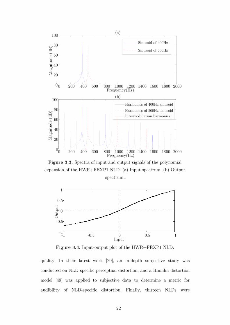
audibility of NLD-specific distortion. Finally, thirteen NLDs were

Mag

nit

ude

(dB

)

Sinusoid of 400Hz

Sinusoid of 500Hz

Harmonics of 400Hz sinusoid

Harmonics of 500Hz sinusoid

Intermodulation harmonics

Frequency(Hz)

Mag

nit

ude

(dB

)

0 200 400 600 800 1000 1200 1400 1600 1800 20000

20

40

60

80

100

(a)

(b)

0

20

40

60

80

100

Frequency(Hz)0 200 400 600 800 1000 1200 1400 1600 1800 2000

Figure 3.3. Spectra of input and output signals of the polynomial

expansion of the HWR+FEXP1 NLD. (a) Input spectrum. (b) Output

spectrum.

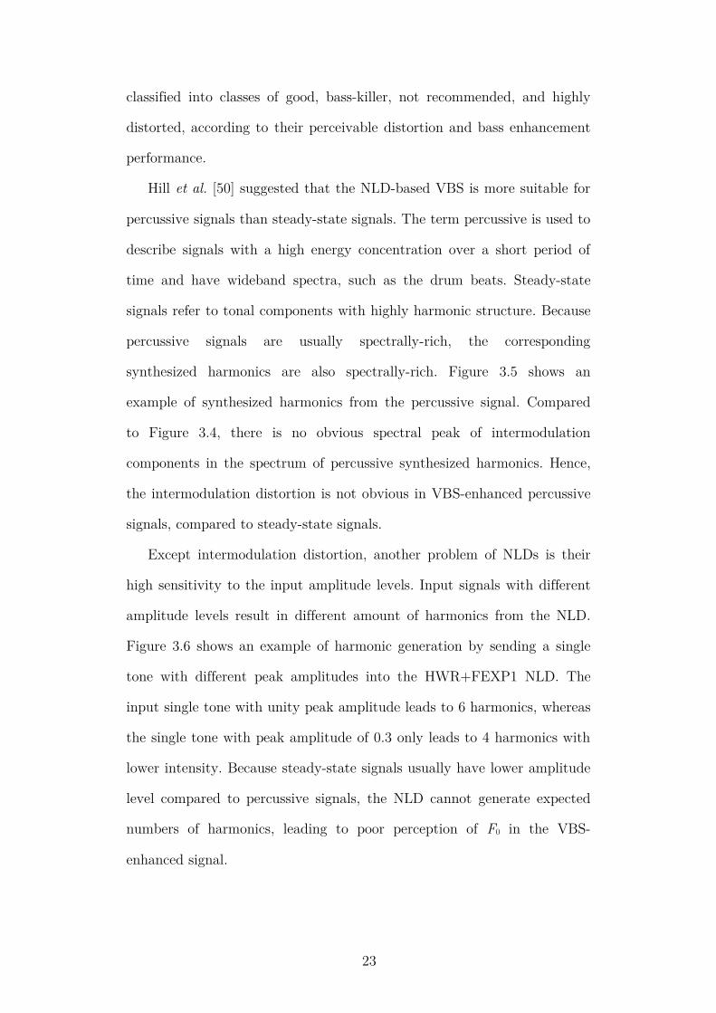
Input

Outp

ut

-1 -0.5 0 0.5 1-1

-0.5

0

0.5

1

Figure 3.4. Input-output plot of the HWR+FEXP1 NLD.

23

classified into classes of good, bass-killer, not recommended, and highly

distorted, according to their perceivable distortion and bass enhancement

performance.

Hill et al. [50] suggested that the NLD-based VBS is more suitable for

percussive signals than steady-state signals. The term percussive is used to

describe signals with a high energy concentration over a short period of

time and have wideband spectra, such as the drum beats. Steady-state

signals refer to tonal components with highly harmonic structure. Because

percussive signals are usually spectrally-rich, the corresponding

synthesized harmonics are also spectrally-rich. Figure 3.5 shows an

example of synthesized harmonics from the percussive signal. Compared

to Figure 3.4, there is no obvious spectral peak of intermodulation

components in the spectrum of percussive synthesized harmonics. Hence,

the intermodulation distortion is not obvious in VBS-enhanced percussive

signals, compared to steady-state signals.

Except intermodulation distortion, another problem of NLDs is their

high sensitivity to the input amplitude levels. Input signals with different

amplitude levels result in different amount of harmonics from the NLD.

Figure 3.6 shows an example of harmonic generation by sending a single

tone with different peak amplitudes into the HWR+FEXP1 NLD. The

input single tone with unity peak amplitude leads to 6 harmonics, whereas

the single tone with peak amplitude of 0.3 only leads to 4 harmonics with

lower intensity. Because steady-state signals usually have lower amplitude

level compared to percussive signals, the NLD cannot generate expected

numbers of harmonics, leading to poor perception of F0 in the VBS-

enhanced signal.

24

3.2 Implementation of the PV in the VBS

The PV-based VBS uses the pitch-shifting function of the PV to

generate higher harmonics. The fundamental assumption of the PV is that

the input signal can be modeled as a sum of slowly varying sinusoids:

(3.2)

ϕk and Ak(n) and fk(n) are the instantaneous phase, amplitude

0 200 400 600 800 10000

10

20

30

40

50

60original

hamronics

Frequency(Hz)

Mag

nit

ude

(dB

)

Figure 3.5. Synthesized harmonics of a percussive signal using the

polynomial expansion of the HWR+FEXP1 NLD.

0 100 200 300 400 500 600 700 8000

10

20

30

40

50

60

70

80

90

100

Frequency (Hz)

Mag

nit

ude

(dB

)

0

10

20

30

40

50

60

70

80

90

100

Mag

nit

ude

(dB

)

0 100 200 300 400 500 600 700 800Frequency (Hz)

(b)(a)

polynomial expansion of the HWR+FEXP1

25

and frequency of the kth sinusoid, respectively; I(n) is the number of

sinusoids, and fs is the sampling frequency,

The spectrum 𝑋𝑃𝑉 (𝑚, 𝑘) of the input signal is obtained using short-

time Fourier transform (STFT) [43]. The frame of input samples is

multiplied by a window function h(n), which is slid along the time axis,

before being transformed to frequency domain:

(3.3)

where m is the frame index and k is the frequency bin index, Lwin and Ra

are the analysis frame length and hop size, respectively. Figure 3.7 shows

an example of successive windowed frames along the time axis.

The spectrum consists of the magnitude spectrum |𝑋𝑃𝑉 (𝑚, 𝑘)| and the

phase spectrum ∠𝑋𝑃𝑉 (𝑚, 𝑘). In the PV, the amplitude of pitch-shifted

signal is determined by the |𝑋𝑃𝑉 (𝑚, 𝑘)|, and the instantaneous

frequencies of the input signal are estimated based on the ∠𝑋𝑃𝑉 (𝑚, 𝑘).

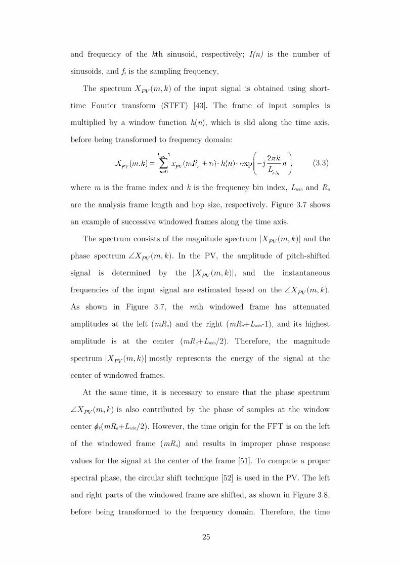
As shown in Figure 3.7, the mth windowed frame has attenuated

amplitudes at the left (mRa) and the right (mRa+Lwin-1), and its highest

amplitude is at the center (mRa+Lwin/2). Therefore, the magnitude

spectrum |𝑋𝑃𝑉 (𝑚, 𝑘)| mostly represents the energy of the signal at the

center of windowed frames.

At the same time, it is necessary to ensure that the phase spectrum

∠𝑋𝑃𝑉 (𝑚, 𝑘) is also contributed by the phase of samples at the window

center ϕk(mRa+Lwin/2). However, the time origin for the FFT is on the left

of the windowed frame (mRa) and results in improper phase response

values for the signal at the center of the frame [51]. To compute a proper

spectral phase, the circular shift technique [52] is used in the PV. The left

and right parts of the windowed frame are shifted, as shown in Figure 3.8,

before being transformed to the frequency domain. Therefore, the time

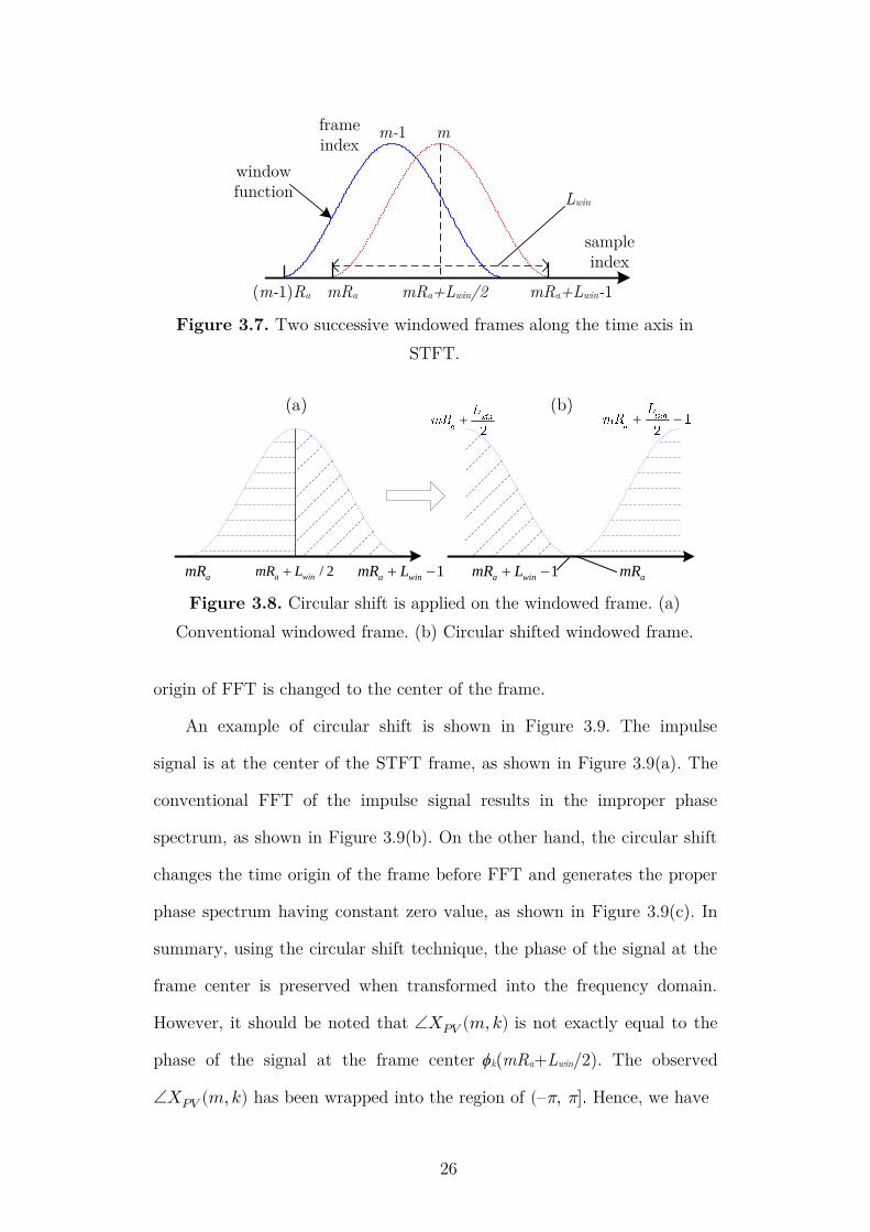
26

origin of FFT is changed to the center of the frame.

An example of circular shift is shown in Figure 3.9. The impulse

signal is at the center of the STFT frame, as shown in Figure 3.9(a). The

conventional FFT of the impulse signal results in the improper phase

spectrum, as shown in Figure 3.9(b). On the other hand, the circular shift

changes the time origin of the frame before FFT and generates the proper

phase spectrum having constant zero value, as shown in Figure 3.9(c). In

summary, using the circular shift technique, the phase of the signal at the

frame center is preserved when transformed into the frequency domain.

However, it should be noted that ∠𝑋𝑃𝑉 (𝑚, 𝑘) is not exactly equal to the

phase of the signal at the frame center ϕk(mRa+Lwin/2). The observed

∠𝑋𝑃𝑉 (𝑚, 𝑘) has been wrapped into the region of (–π, π] Hence, we have

mm-1frame index

sample index

Lwin

mRa+Lwin-1(m-1)Ra mRa+Lwin/2mRa

window function

Figure 3.7. Two successive windowed frames along the time axis in

STFT.

/ 2a winmR L 1a winmR L amR

0 500 1000 1500 2000 2500 3000-0.5

0

0.5

1

1.5

amR 1a winmR L

0 500 1000 1500 2000 2500 3000-0.5

0

0.5

1

1.5

0 500 1000 1500 2000 2500 3000-0.5

0

0.5

1

1.5

0 500 1000 1500 2000 2500 3000-0.5

0

0.5

1

1.5

(a) (b)

Figure 3.8. Circular shift is applied on the windowed frame. (a)

Conventional windowed frame. (b) Circular shifted windowed frame.

27

(3.4)

where u is an unknown integer.

The instantaneous frequency fk(n) is estimated based on ∠𝑋𝑃𝑉 (𝑚, 𝑘)

of successive frames. With (3.2) and (3.4), we can link fk(n) and

∠𝑋𝑃𝑉 (𝑚, 𝑘) as:

(3.5)

To estimate fk(n) from the spectral phase, it is necessary to remove the

(b)

(c)

Frequency (Hz)

Frequency (Hz)

Phas

e (r

adia

ns)

Phas

e (r

adia

ns)

Time (sec)

Am

plitu

de

(a)

0 0.5 1 1.5 2 x 104-1

-0.5

0

0.5

1

0 0.004 0.008 0.012 0.016 0.020

0.2

0.4

0.6

0.8

1

0 0.5 1 1.5 2 x 104-4

-2

0

2

4

Figure 3.9. Phase spectrum of an impulse signal. (a) Plots of the impulse

signal at the center of the STFT frame. (b) Phase spectrum without

circular shift. (c) Phase spectrum with circular shift.

28

unknown part 2uπ. Assuming that the analysis window is long enough

that each frequency bin only contains one sinusoid, as shown in Figure

3.10, the instantaneous frequencies are limited in the region of each

frequency bin:

(3.6)

With the constraint in (3.6), we can express (3.5) as

(3.7)

Because the hop size Ra is always smaller than the window length Lwin., we

have:

(3.8)

Equation (3.8) shows that the unknown part -2uπ wraps the phase

∠𝑋𝑃𝑉 (𝑚, 𝑘) − ∠𝑋𝑃𝑉 (𝑚 − 1, 𝑘) − 2𝜋(𝑘 − 1)𝑅𝑎/𝐿𝑤𝑖𝑛 into the region of [0,

2π]. This process of wrapping can be expressed using the principal

argument (PA):

m

k-1

k

Time frames

Fre

quen

cy c

han

nel

s

Figure 3.10. The sinusoid located in frequency bins of the PV.

29

(3.9)

where PA returns the remainder after dividing by 2π, as shown in Figure

3.11. With (3.9), we can remove the unknown part 2uπ in (3.5) and

estimate the instantaneous frequency as:

(3.10)

Subsequently, higher harmonics are synthesized by shifting the

estimated instantaneous frequency according to harmonics’ orders. Earlier

studies of PV-based VBS [21], [50] used a sum-of-sinusoids method [51] to

synthesize harmonics, and a sinusoid oscillator was used to generate the

output signal y𝑃𝑉 (𝑛):

(3.11)

π

3π

2π

0

-π

Outp

ut

phas

e

-6π -4π -2π 0 2π 4π 6πInput phase

Figure 3.11. Principle argument (PA) function.

30

where 𝐴𝑘𝑠(𝑛) and 𝜙𝑘

𝑠(𝑛) are the synthesized magnitude and phase,

respectively.

In the sum-of-sinusoids method, the spectral magnitude the input

signal is used as the synthesized magnitude:

(3.12)

The synthesized phase is obtained based on the phase relationship of

successive frames shown in (3.5), and the estimated instantaneous

frequency in (3.10):

(3.13)

where α is the order of the synthesized harmonic. However, (3.12) and

(3.13) only compute the synthesized magnitude and phase at the center of

the frame. Synthesized samples between centers of successive frames are

calculated using linear interpolation, as shown in Figure 3.12. The

interpolated synthesized magnitude and phase can be calculated as:

(3.14)

and

(3.15)

31

for (m-1)Ra+Lwin/2<n<mRa+Lwin/2. Finally, the synthesized signal is

generated using the sinusoid oscillator in (3.11).

The PV is based on the assumption that the input signal can be

modeled as a sum of slowly varying sinusoids in the spectrum, which

requires an adequate frequency resolution [53]. In STFT, relationship

between the frame size Lwin and frequency resolution fres is

(3.16)

For accurate frequency analysis of input signals, a small fres is required,

leading to a large frame size Lwin. However, large frame length reduces the

time resolution and may soften (smear) the pitch-shifted percussive

components [53]. Previous solutions, such as phase handling methods [54]–

[56] and the re-insertion method for percussive components [41], are all

aimed at the PV for time-scaling but not for pitch-shift. A constant-Q

transform (CQT) based PV [53] can mitigate this problem by providing a

very good time resolution at high-frequencies, but it cannot solve the

smearing problem for low-frequency percussive components.

On the other hand, the PV has no intermodulation distortion as in the

Linear

Interpolation

Figure 3.12. Linear interpolation of the synthesized amplitude 𝐴𝑘𝑠(𝑛)

and phase 𝜙𝑘𝑠(𝑛) between successive frames.

32

NLD. In addition, accurate control is provided by the PV over each

synthesized harmonic. Therefore, the problem of input amplitude

sensitivity is avoided, and the PV can generate expected numbers of

harmonics for steady-state signals with lower amplitude levels. In

summary, the PV-based VBS is more appropriate for the steady-state

signal than the percussive signal.

3.3 Hybrid Virtual Bass System

As mentioned above, both NLD and PV have their own unique

advantages and drawbacks in the VBS. Problems of intermodulation

distortion and input-sensitivity from the NLD are more distinct for

steady-state signals compared to percussive signals; whereas the PV is not

suitable for percussive signals due to the trade-off between time and

frequency resolutions. Therefore, the idea of the hybrid VBS, which

combines NLD and PV, was proposed by Hill and Hawksford in [50], and

Mu and Gan in [57].

3.3.1 Earlier Studies on Hybrid VBS

The hybrid VBS has the respective advantages of NLD and PV, and

circumvents each other’s weaknesses, forming a less sensitive system to

input signal contents. From the subjective evaluation, Hill’s hybrid VBS

[50] was found to be more robust in processing various genres of music

compared to the individual NLD-based and PV-based VBS.

General framework of Hill’s hybrid VBS is shown in Figure 3.13. A

transient content detector (TCD) was designed to handle the mixing of

NLD’s and PV’s outputs. The TCD analyzes the input signal and assigns

the appropriate weights (wNLD and wPV in Figure 3.13) to the outputs of

PV and NLD that are running in parallel. When the input signal contains

33

more percussive contents, the hybrid VBS favors the NLD output.

Conversely, the PV output is utilized when the input signal is

predominantly steady-state.

More specifically, the TCD tracks the change of spectral energy

between successive frames. When change of spectral energy between

successive fames exceeds a certain threshold, the weights for PV and NLD

(wPV and wNLD in Figure 3.13) are decreased and increased, respectively, as

shown in Figure 3.14. The sum of weights wPV and wNLD is one. This

algorithm is based on the fact that the percussive signals usually have a

sudden change of energy as compared to steady-state signals.

However, Hill’s separation method may not effectively separate the

harmonics from percussive and steady-state components, especially for

input signals with both heavy percussive and steady-state components. As

shown in Figure 3.14, the weighting curves (wPV and wNLD) vary slowly

between the two components, and the weight wNLD does not reach 1 during

the peak of percussive components. Due to the ineffective separation,

synthesized harmonics are still contributed by both suitable and

unsuitable harmonic generators, and distortions (to a lesser extent) still

exist. An objective evaluation on the separation performance of Hill’s

NLD

PV

+

inputsignal

TCD

BPF

HPF

outputsignal

×

×

LPF

LPF

G+

wPV

wNLD

Figure 3.13. General framework of Hill’s hybrid VBS.

34

method will be introduced in Section 3.5.

In the next section, we propose a new hybrid VBS [57], which

overcomes the drawbacks of Hill’s method and achieves a better

performance of the separation for steady-state and percussive components.

3.3.2 New Hybrid VBS

The general framework of the proposed hybrid VBS is shown in Figure

3.15. Different from Hill’s method with weight assignment for outputs of

different harmonic generators, the proposed hybrid system separates the

spectrum of the input signal into percussive and steady-state components,

and then applies NLD and PV on the respective components.

In the proposed hybrid system, we use a median filter based separation

(a)

(b)

0 1 2 3 4 5 6 7 8 9 100

0.2

0.4

0.6

0.8

1

0 1 2 3 4 5 6 7 8 9 100

0.2

0.4

0.6

0.8

1

0 1 2 3 4 5 6 7 8 9 10-1

-0.5

0

0.5

1

(c)

Time (sec)

wPV

wN

LD

Am

plitu

de

Figure 3.14. Example of TCD weighting functions. (a) Input signal. (b)

Weighting curve wNLD for the NLD. (c) Weighting curve wPV for the PV.

35

method introduced in [58], which is based on the fact that the steady-

state component appears as a horizontal ridge in the magnitude

spectrogram, whereas the percussive component forms a vertical ridge (see

Figure 3.16). When the median filter is applied across the time axis, it

smoothens out the horizontal (steady-state) lines and filters out the

vertical (percussive) lines, producing steady-state-enhanced components

SMF(m,k). Similarly, percussive-enhanced components PMF(m,k) are

produced when median filter is applied across the frequency axis.

The general structure of the proposed separation method is shown in

Figure 3.17. To avoid artifacts introduced by the nonlinearity of the

median filter, the enhanced spectra SMF(m,k) and PMF(m,k) from the

median filter are used to generate the soft separation masks. The

spectrum separation masks for the percussive component MP(m,k) and the

steady-state component MS(m,k) are generated using

(3.17)

Finally, the percussive Px(m,k) and steady-state Sx(m,k) spectrograms can

STFTPercussive / Steady-

state separation

NLD

PV

+

+

LPF

LPF

HPF

output signal

BPF

Px(m,k)

Sx(m,k)

ISTFT

G

inputsignal

xHF(n)

xHA(n)

y(n)

x(n)

percussive

steady-state

Figure 3.15. Framework of the proposed hybrid VBS.

36

be extracted by multiplying the input spectrum X(m,k) with the masks:

(3.18)

Figure 3.18 shows the results of the proposed separation method using the

spectrogram in Figure 3.16. The percussive and steady-state spectrograms

are clearly separated. In addition, since the masks only operate on the

magnitude spectrum, the phase information of the separated spectra is

Percussive

Steady-state

Time

Fre

quen

cy

Figure 3.16. The spectrum of a musical signal with both percussive and


×

×

Percussive

Steady-state

Median filter

Median filter

Maskgenerator

Fre

quen

cy

Time

Figure 3.17. Framework of the percussive and steady-state separation

using the proposed method. Masks are generated by (3.17).

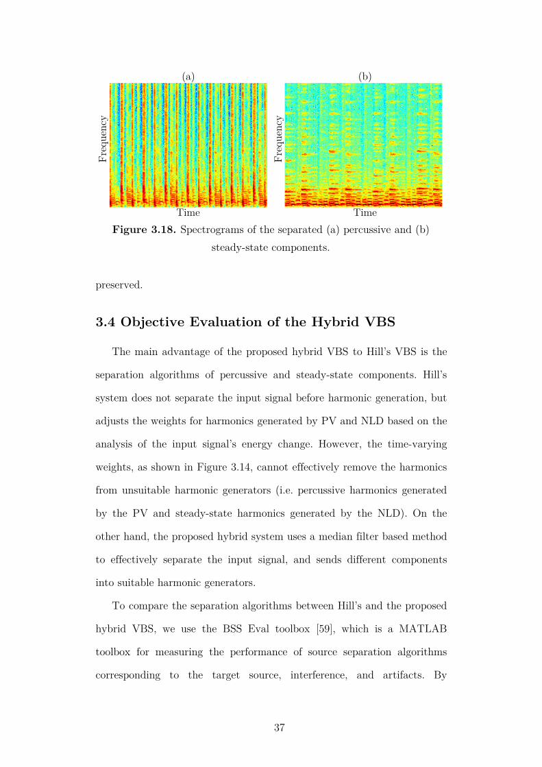
37

preserved.

3.4 Objective Evaluation of the Hybrid VBS

The main advantage of the proposed hybrid VBS to Hill’s VBS is the

separation algorithms of percussive and steady-state components. Hill’s

system does not separate the input signal before harmonic generation, but

adjusts the weights for harmonics generated by PV and NLD based on the

analysis of the input signal’s energy change. However, the time-varying

weights, as shown in Figure 3.14, cannot effectively remove the harmonics

from unsuitable harmonic generators (i.e. percussive harmonics generated

by the PV and steady-state harmonics generated by the NLD). On the

other hand, the proposed hybrid system uses a median filter based method

to effectively separate the input signal, and sends different components

into suitable harmonic generators.

To compare the separation algorithms between Hill’s and the proposed

hybrid VBS, we use the BSS Eval toolbox [59], which is a MATLAB

toolbox for measuring the performance of source separation algorithms

corresponding to the target source, interference, and artifacts. By

(a) (b)

Time

Fre

quen

cy

Time

Fre

quen

cy

Figure 3.18. Spectrograms of the separated (a) percussive and (b)


38

analyzing the target source signals and separated signals, the BSS Eval

toolbox gives three performance criteria, including source-to-interferences

ratio (SIR), sources-to-artifacts ratio (SAR), and source-to-distortion (the

sum of interference, artifacts and remaining sensor noise) ratio (SDR). All

of the criteria are expressed in decibels (dB).

Two sets of stimuli from the development stimuli of Signal Separation

Evaluation Campaign (SiSEC) 2011 [60] and two sets of generated stimuli

with bass guitar (from [61]) and kick drum (from [62]) were used. In each

set, a percussive stimulus and a steady-state stimulus were mixed and

sent into the two separation algorithms. Separated signals in Hill’s system

were generated by multiplying the TCD weights to the mixed signals, as

shown in Figure 3.19. In the proposed system, output signals of the

median filter based separation (Sx(m,k) and Px(m,k) in Figure 3.17) were

transformed into the time domain using inverse short-time Fourier

transform (ISTFT). All the original and separated stimuli can be found in

Appendix C.

The evaluation result is shown in Table 3.1. It is found that the

proposed separation method outperforms Hill’s method in most of the

criteria. The SDR of most the separated components are increased by

inputsignal

TCD

×

×

wPV

wNLD

separated steady-state signal

separated percussive signal

Figure 3.19. Separation of steady-state and percussive signals using

Hill’s method.

39

using the proposed separation method. The most significant improvements

from the proposed method are SAR of the separated percussive signal and

SIR of the separated steady-state signal. Using the proposed separation

method, SIRs of separated steady-state signals are increased by 5 dB to

17 dB in three stimuli, and SARs of the separated percussive signal are

increase by 2 dB to 26 dB in all the stimuli.

An example of separation (Stimulus 2 in Table 3.1) is shown in

Table 3.1. Evaluation results of Hill’s and the proposed separation

method.

Stimulus 1 (dev2__ultimate_nz_tour)

Steady-state Percussive

SDR(dB) SIR(dB) SAR(dB) SDR(dB) SIR(dB) SAR(dB)

Hill 2.56 2.34 5.92 2.79 3.56 3.20

Proposed 2.85 10.67 3.58 7.73 10.58 10.85

Stimulus 2 (dev1__bearlin-roads)



Hill 8.01 12.84 9.96 2.07 4.71 0.22

Proposed 9.95 29.92 10.00 2.75 6.20 6.30

Stimulus 3 (bass guitar + kick drum)



Hill 1.90 10.72 2.87 5.16 3.37 4.56

Proposed 4.19 6.28 9.28 7.01 5.08 30.70

Stimulus 4 (bass guitar + kick drum)


SDR(dB) SIR(dB) SAR(dB) SDR SIR SAR

Hill 2.92 17.91 3.13 8.79 7.14 4.12

Proposed 7.18 22.31 7.34 6.62 5.48 6.26

40

Figure 3.20. Compared to the proposed separation method, the lower SIR

of steady-state signals in Hill’s system is due to the fact that the time-

varying weight curves cannot effectively separate the two components. As

shown in Figure 3.20(c), the steady-state signals from Hill’s method still

contain some percussive components. On the other hand, the proposed

method can effectively filter out the percussive components, as shown in

Figure 3.20(e). Although the separated percussive signals from the

proposed method still contain some steady-state components, the SIR of

percussive signals is less affected due the fact that the energy of percussive

signals is generally much higher than steady-state signals. In addition, in

0 2 4 6 8 10 12-1

-0.5

0

0.5

1

0 2 4 6 8 10 12-1

-0.5

0

0.5

1

0 2 4 6 8 10 12-1

-0.5

0

0.5

1

0 2 4 6 8 10 12-1

-0.5

0

0.5

1

0 2 4 6 8 10 12-1

-0.5

0

0.5

1

0 2 4 6 8 10 12-1

-0.5

0

0.5

1

Time (sec)Time (sec)

Am

plitu

de

Am

plitu

de

Am

plitu

de

(a)

(c)

(e) (f)

(d)

(b)

leaked percussive components

artifacts

Figure 3.20. Comparison between Hill’s and the proposed separation

methods for steady-state and percussive components. (a) and (b):

Original steady-state and percussive signals. (c) and (d): Separation

results using Hill’s method. (e) and (f): Separation results using the

proposed method.

41

Hill’s method, some steady-state signals that are incorrectly separated

form some artifacts in the separated percussive signal (as shown in Figure

3.20(d)), leading to a low SAR of the separated percussive signal.

3.5 Chapter Summary

In this chapter, two commonly used harmonic generators in the VBS,

the nonlinear device (NLD) and the phase vocoder (PV), were described

in detail. The NLD and the PV have their own unique advantages and

drawbacks, and are more applicable for percussive and steady-state signals,

respectively. Therefore, a hybrid VBS, which combines two harmonic

generators (NLD and PV), was proposed as a solution to overcome the

shortcomings of the VBS using the single harmonic generator. The hybrid

VBS separates the input signal into percussive and steady-state

components, and uses different approaches to generate harmonics. Earlier

research had similar idea of using two harmonic generators, but their

system cannot effectively separate the input signal into percussive and

steady-state components. Objective testing results showed that the

proposed separation method was much more effective than the previous

method. The subjective test that compares different types of VBS will be

introduced in Chapter 6.

In the next two chapters, we will introduce VBS techniques to further

improve the quality of steady-state components (in Chapter 4) and to

overcome the overflow problem for percussive components (in Chapter 5).

42

Quality Improvement for the

Phase Vocoder

The previous chapter introduced a hybrid VBS that combines NLD and

PV to generate harmonics for different components of the input signal. In

the hybrid VBS, steady-state components of the input signal are extracted

and sent into the PV. In this chapter, an improved harmonic synthesis

approach (in Section 4.1) and a timbre matching scheme (in Section 4.2)

are proposed for improving the quality of harmonics from the PV.

Compared to the conventional PV in the VBS, the improved PV proposed

in Section 4.1 leads to fewer distortions in synthesized harmonics. In

Section 4.2, we propose a new weighting scheme for the PV based on the

timbre information, which can reduce the unnatural sharpness effect of

synthesized harmonics. Finally, Section 4.3 summarizes the main findings

in this chapter.

4.1 Improved Harmonic Synthesis in the PV

Section 3.2 introduced a type of PV that uses the sinusoidal oscillator

for harmonic generation. As stated in Section 3.2, the PV operates on the

spectrum of the input signal. The spectrum is obtained by taking the

Fourier transform of a frame of signal samples multiplied with an analysis

window, as shown in (3.3). According to the convolution theorem, the

spectrum of a windowed sinusoid at frequency fk is the spectrum of the

43

analysis window with its main-lobe centered at frequency fk [63], as shown

in Figure 4.1(a) and (b). Hence, the spectral peak of a sinusoid may

occupy more than one frequency bin. However, the sinusoidal oscillator in

the PV regards each frequency bin as an individual sinusoid signal and

synthesizes pitch-shifted signals from all the frequency bins. Therefore, the

synthesized signal of the PV may have spectral distortions around the

frequency bin of the spectral peak, as shown in Figure 4.1(c) and (d).

As the conventional PV introduces spectral distortions in synthesized

harmonics, some other types of PV for pitch-shifting are studied here in

the context of the VBS. One common approach is to time-scale the input

signal using the PV, followed by sampling rate conversion to restore the

signal’s original time duration and modify its frequencies [53]. The PV

implements time-scaling by using different analysis and synthesis hop sizes

0 0.01 0.02 0.03 0.04 0.05 0.06 0.07 0.08 0.09-1

-0.8

-0.6

-0.4

-0.2

0

0.2

0.4

0.6

0.8

1

Fourier transform

Am

plitu

de

Time (sec)

(a) (b)

0 100 200 300 400 500 600 700 800

Mag

nit

ude

(dB

)-40

-20

0

20

40

60

80

-40

-20

0

20

40

60

80

Mag

nit

ude

(dB

)0 100 200 300 400 500 600 700 8000 0.01 0.02 0.03 0.04 0.05 0.06 0.07 0.08 0.09

Time (sec)-1

-0.8

-0.6

-0.4

-0.2

0

0.2

0.4

0.6

0.8

1

Am

plitu

de

Frequency (Hz)

Frequency (Hz)

(c) (d)

Fourier transform

shifted signal. (d) Spectrum of the pitch-shifted signal.

44

[47] or copying and deleting time frames [64]. However, computational

demands become increasingly large by using the resampling method for

higher order pitch-shifting [46]. Hence, repeated processing of generating

second to sixth harmonics requires a prohibitive cost for real-time

applications. In addition, the time-scaling using the PV suffers from some

perceptual artifacts, often described as “phasiness,” “reverberation,” or

“loss of presence” [47].

In 1999, an improved PV technique was introduced by Laroche et al.

[46] for pitch-shifting, which directly manipulates signals in the spectrum.

As mentioned above, sinusoids in signals can be represented by spectral

peaks in the frequency domain. This method identifies the spectral peaks

by picking the local maximum in the spectrum. Next, the spectrum is

divided into influence regions centered on the identified spectral peaks.

The border of the adjacent regions is set as the nulls between the two

peaks. All frequency bins within the influence region contribute to the

same sinusoid related to its spectral peak. This improved PV generates

the spectrum of higher harmonics by shifting influence regions to the

frequencies of higher harmonics. Assuming that the instantaneous

frequency of the spectral peak is fp, all the frequency bins in the

corresponding region are shifted by the distance (α-1)fp, where α is the

higher harmonic’s order. The instantaneous frequency can be estimated

based on the phase information, as discussed in Section 3.2. Figure 4.2

shows an example of pitch-shifting with α = 2, and each influence region

is shifted according to its own Finally, time-

domain harmonics are generated by transforming the spectrum using

inverse short-time Fourier transform (ISTFT).

The improved PV can efficiently avoid spectral distortions that occur

45

in the previous PV used for the VBS. However, the audio quality of

harmonics that are synthesized in frequency domain is highly related to

the phase coherence [46], [47], [53]. The phase spectrum of synthesized

harmonics should be suitably adjusted to avoid phase propagation errors.

The phase coherence of the spectrum consists of horizontal phase

coherence (phase across time frames) and vertical phase coherence (phase

across frequency bins). Laroche et al. [46] introduced a vertical phase

locking scheme, which is based on the fact that a constant amplitude and

frequency sinusoid (with the circular shift mentioned in Section 3.2)

exhibits identical phases in the spectral peak and all nearby bins, as

shown in Figure 4.3. The phase spectrum (with the circular shift) of a 250

Hz sinusoid has an identical phase of 0.167π in the frequency bins from

240.2 Hz to 260.7 Hz. Hence, to get high quality synthesized signals, this

phase relation between spectral peak and the neighboring bins in the

phase spectrum ∠𝑋𝑃𝑉 (𝑚, 𝑘) of the input signal should be preserved in

the synthesized phase spectrum ∠𝑌𝑃𝑉 (𝑚, 𝑘) as:

(4.1)

for all the frequency bins k that belongs to the same influence region of

the spectral peak kp.

Besides Laroche’s vertical phase coherence maintenance approach, we

5

10

15

20

25

0 100 200 300 400 500 600 700 800 900 10000

5

10

15

20

25

Shift

by 2

Mag

nit

ude

Frequency (Hz) Frequency (Hz)

f1

f2

2f1

2f2

Mag

nit

ude

0 100 200 300 400 500 600 700 800 900 10000

Region 1Region 2

Region 1Region 2

Figure 4.2. Use the proposed PV to shift the spectrum by two.

46

propose a maintenance approach for horizontal phase coherence in the PV.

In pitch-shifting, the instantaneous frequency of synthesized harmonics

𝑓𝑘𝑠(𝑛) is

(4.2)

where α is the order of the synthesized harmonic, and fk(n) is the

instantaneous frequency of the input signal. According to the sinusoid

model in (3.2), the synthesized instantaneous phase 𝜙𝑘𝑠(𝑛) is given as

(4.3)

We set the initial synthesized phase as

(4.4)

where ϕk(n) is the instantaneous phase of the input signal. The

synthesized instantaneous phase of the shifted sinusoid with horizontal

phase coherence becomes:

0 100 200 300 400 500 600 700 800-1

-0.5

0

0.5

1

Phas

e (π

)

Frequency (Hz)

240.2 Hz 260.7 Hz

Figure 4.3. Phase spectrum of a 250 Hz sinusoid.

47

(4.5)

As mentioned above, sinusoids are represented by spectral peaks in the

proposed PV. Based on (3.4), the horizontal phase coherence of the

synthesized spectrum can be maintained by satisfying

(4.6)

where ∠𝑌𝑃𝑉 (𝑚, 𝑘𝑝) is the synthesized phase spectrum at the mth frame

and the frequency bin of spectral peak kp, and ∠𝑋𝑃𝑉 (𝑚, 𝑘) is the input

phase spectrum. Because α, u and 𝑢′ in (4.6) are all integers, the term

2𝛼(u − 𝑢′)𝜋 is the integral multiple of 2π and can be dropped in the

computation of phase. Therefore, the synthesis phase coherence across

time frames in the proposed PV can be preserved by satisfying

(4.7)

Figure 4.4 shows an example of the PV with and without phase

coherence maintenance. Note that the attenuation at the beginning and

end of synthesized signals is due to the window function of ISTFT. Figure

4.4(b) is the pitch-shifted sinusoid by shifting the magnitude spectral peak

but using the original phase spectrum. Compared to the synthesized

sinusoid with phase coherence maintenance shown in Figure 4.4(c), there

is an undesired change in the amplitude envelope of the pitch-shifted

sinusoid without phase coherence maintenance. Laroche et al. [47]

mentioned that this kind of amplitude modulation in the synthesized

48

signal of the PV is due to the lack of phase coherence. We also found that

the lack of vertical phase coherence does not result in the envelope change

on the tested sinusoid, as shown in Figure 4.4(d). As mentioned by

Laroche et al. [65], the vertical phase locking is introduced to solve the

phasiness problem, which mainly occurs in complex signals, especially in

speech signals.

In summary, the proposed PV synthesizes the harmonics in the

frequency domain, and hence it overcomes the problem of spectral

distortions in the conventional PV that uses sinusoidal oscillator. In

addition, we proposed an approach to maintain the phase coherence of the

synthesized signal in the PV. Therefore, the proposed PV can be used to

0 0.05 0.1 0.15 0.2-1

-0.5

0

0.5

1

0 0.05 0.1 0.15 0.2-1

-0.5

0

0.5

1

0 0.05 0.1 0.15 0.2-1

-0.5

0

0.5

1

0 0.05 0.1 0.15 0.2-1

-0.5

0

0.5

1

Time(sec) Time(sec)

Am

plitd

ue

Am

plitd

ue

(b)

(d)

(a)

(c)

Figure 4.4. Use the PV to shift a single tone by three, with and without

phase coherence maintenance. (a) Input 250 Hz sinusoid signal. (b) Pitch-

shifted signal without phase coherence maintenance. (c) Pitch-shifted

signal with both horizontal and vertical phase coherence maintenance. (d)

Pitch-shifted signal with only horizontal phase coherence maintenance.

49

improve the audio quality of the VBS.

4.2 Harmonic Weighting Schemes

Additional harmonics in the VBS increases the audio sharpness of the

original signal, which is a perception related to the spectral density [37].

Suitable weighting schemes should be applied to control the magnitudes of

additional harmonics. Otherwise, the output signal may have unnatural

sharpness effect, which heavily reduces the perceptual quality [2]. For the

NLD-based VBS, a band-pass filter can be placed after the NLD

processing block to attenuate the harmonics generated by the NLD [2].

However, NLDs are highly sensitive to the input amplitude (as shown in

Figure 3.6), which results in the harmonics’ magnitudes that are not

controllable.

On the other hand, the PV approach in the VBS provides accurate

control over each synthesized harmonic, and magnitude weighting schemes

can be used to produce better quality for steady-state signals in the

proposed VBS. In the PV proposed in Section 4.1, the ith synthesized

harmonic is weighted as:

(4.8)

for frequency bins k belonging to the influence region of the spectral peak

kp. The weight Wi is determined by the weighting scheme, and

|𝑋𝑃𝑉 (𝑚, 𝑘)| refers to the magnitude spectrum of the input signal of the

PV.

4.2.1 Loudness Matching Scheme

Earlier research on the PV-based VBS [21] used a loudness matching

scheme, which weights the harmonics based on equal-loudness contours.

The idea of this scheme is to generate harmonics having the same

50

loudness as the target fundamental frequency. In this approach, equal-

loudness curves are parameterized by [66]:

(4.9)

where Loudn(f) and SPL( f ) represent the loudness in phon and the sound

pressure level (SPL) in dB at the frequency f, respectively. The frequency

dependent parameters af, bf, and Tf are fitted into polynomials to reduce

memory requirement. The polynomials are accurate for frequencies lower

than 2 kHz, and the coefficients are given in [21]:

(4.10)

Based on (4.9), the SPL of the ith harmonic having the same loudness as

the fundamental frequency F0 is estimated by solving the following

equation:

(4.11)

where SPL(i∙F0) and SPL(F0) denote the SPL of the ith harmonic and F0,

respectively. Finally, the weighting ratio of the ith harmonics is

determined by:

(4.12)

It should be noted that this scheme adjusts the individual harmonic to

have the same loudness at F0. The combination of the second to sixth

harmonics still has different loudness compared to the loudness of F0.

51

4.2.2 Fixed Weighting Scheme

In the fixed weighting scheme, Wi are constant for all the input signals.

The exponential attenuation scheme is a commonly used fixed weighting

scheme, which computes the weighting ratio for the ith harmonic as:

(4.13)

where α determines the rate of attenuation of the harmonics’ magnitudes.

To evaluate the effect of α, we compute the 𝑊𝑖𝐸𝑋𝑃 for α = 0.3 and 0.6.

As shown in Figure 4.5, the harmonics attenuate faster when α = 0.6 as

compared to α = 0.3. The amplitudes of the harmonics attenuate by 12

dB and 6 dB for every increment of harmonic’s order in the case of α =

0.6 and 0.3, respectively.

4.2.3 Timbre Matching Scheme

In this section, we propose a timbre matching weighting scheme [67],

which produces harmonics having the similar timbre to the original sound.

According to American Standard Acoustical Terminology [68], timbre is

defined as the “attribute of auditory sensation in terms of which a listener

can judge two sounds similarly presented and having the same loudness

and pitch as dissimilar”. Therefore, similar timbre between VBS-enhanced

and original signal may reduce the perceived distortion caused by

additional harmonics.

Schouten [69] stated that timbre is determined by five major audio

parameters:

1) the range between tonal and noise-like character;

2) the spectral envelope;

3) the time envelope;

4) the changes of spectral envelope and fundamental frequency;

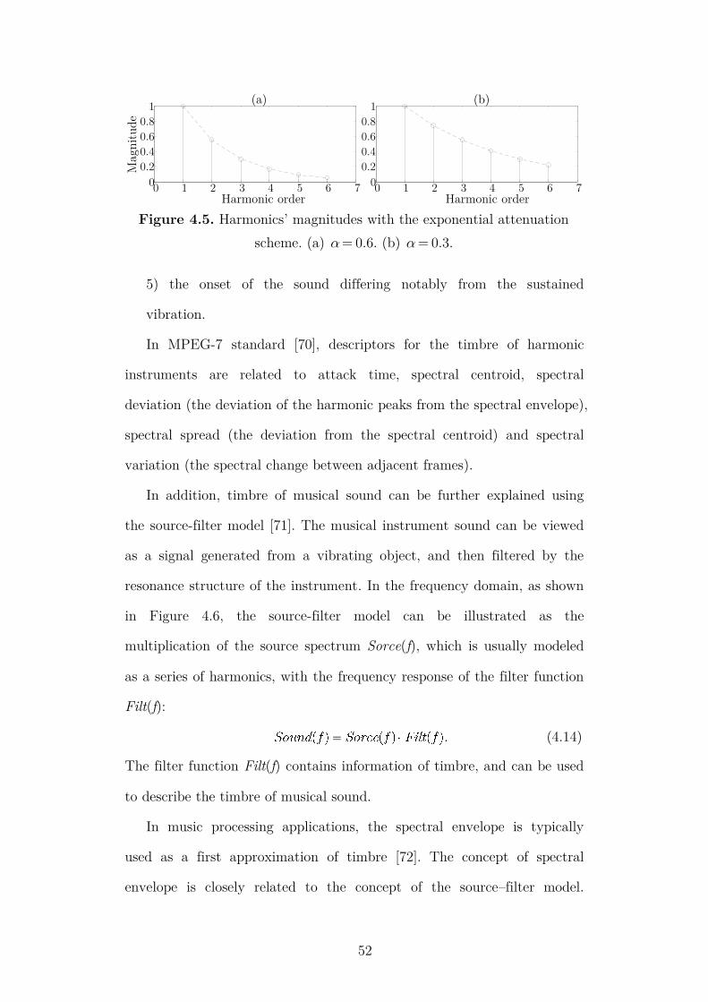
52

5) the onset of the sound differing notably from the sustained

vibration.

In MPEG-7 standard [70], descriptors for the timbre of harmonic

instruments are related to attack time, spectral centroid, spectral

deviation (the deviation of the harmonic peaks from the spectral envelope),

spectral spread (the deviation from the spectral centroid) and spectral

variation (the spectral change between adjacent frames).

In addition, timbre of musical sound can be further explained using

the source-filter model [71]. The musical instrument sound can be viewed

as a signal generated from a vibrating object, and then filtered by the

resonance structure of the instrument. In the frequency domain, as shown

in Figure 4.6, the source-filter model can be illustrated as the

multiplication of the source spectrum Sorce(f), which is usually modeled

as a series of harmonics, with the frequency response of the filter function

Filt(f):

(4.14)

The filter function Filt(f) contains information of timbre, and can be used

to describe the timbre of musical sound.

In music processing applications, the spectral envelope is typically

used as a first approximation of timbre [72]. The concept of spectral

envelope is closely related to the concept of the source–filter model.

0 1 2 3 4 5 6 70

0.2

0.4

0.6

0.8

1

0 1 2 3 4 5 6 70

0.2

0.4

0.6

0.8

1

Mag

nit

ude

Harmonic order Harmonic order

(a) (b)

Figure 4.5. Harmonics’ magnitudes with the exponential attenuation

scheme. (a) α = 0.6. (b) α = 0.3.

53

Spectral envelope ENV(f) of audio signals can be seen as multiplication of

the filter function Filt(f) with the envelope of the source spectrum

ENVsorce(f):

(4.15)

For steady-state signals, the source is a sum of sinusoids, which usually

has a flat spectral envelope [73], [74]:

(4.16)

Hence, the filter function in the source-filter model can be approximated

using the spectral envelope of the signal.

Timbre information contained in the spectral envelope has been widely

used in musical processing. For example, the Mel-frequency cepstral

coefficients (MFCC) [75], which is a popular way of representing the

spectral envelope, has been successfully used for music genre classification

[37], [76]–[80] and instrument recognition [81]–[84]. In addition, all the five

parameters, except the first, in Schouten’s list and the spectral timbre

descriptors in MPEG-7, can be reasonably well covered by the spectral

envelope [72]. Therefore, matching the spectral envelope of synthesized

harmonics to the original signal can help to produce the VBS-enhanced

signal with similar timbre of the original signal and reduce the perceived

distortion.

The estimation method for the spectral envelope of the low-frequency

Frequency

× =

Source

spectrum

Filter

function

Harmonic sound

spectrum

Frequency Frequency

Figure 4.6. Source-filter model of harmonic sound generation.

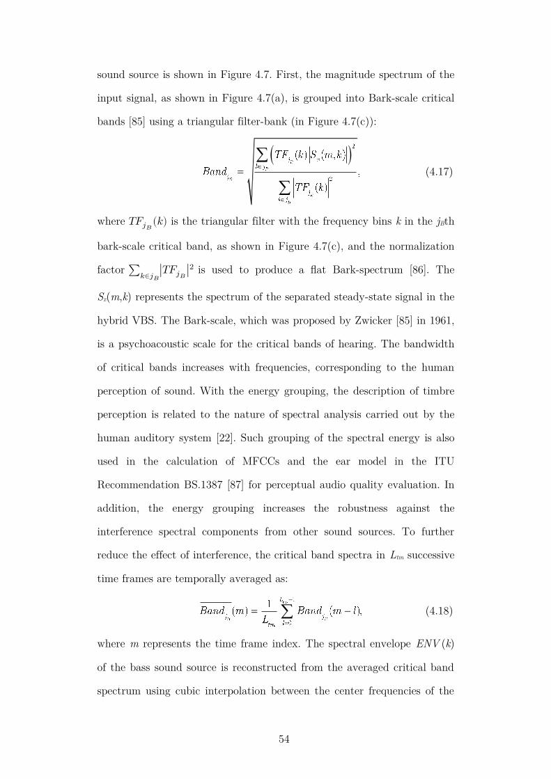
54

sound source is shown in Figure 4.7. First, the magnitude spectrum of the

input signal, as shown in Figure 4.7(a), is grouped into Bark-scale critical

bands [85] using a triangular filter-bank (in Figure 4.7(c)):

(4.17)

where 𝑇𝐹𝑗𝐵(𝑘) is the triangular filter with the frequency bins k in the jBth

bark-scale critical band, as shown in Figure 4.7(c), and the normalization

factor ∑ |𝑇𝐹𝑗𝐵|2

𝑘∈𝑗𝐵is used to produce a flat Bark-spectrum [86]. The

Sx(m,k) represents the spectrum of the separated steady-state signal in the

hybrid VBS. The Bark-scale, which was proposed by Zwicker [85] in 1961,

is a psychoacoustic scale for the critical bands of hearing. The bandwidth

of critical bands increases with frequencies, corresponding to the human

perception of sound. With the energy grouping, the description of timbre

perception is related to the nature of spectral analysis carried out by the

human auditory system [22]. Such grouping of the spectral energy is also

used in the calculation of MFCCs and the ear model in the ITU

Recommendation BS.1387 [87] for perceptual audio quality evaluation. In

addition, the energy grouping increases the robustness against the

interference spectral components from other sound sources. To further

reduce the effect of interference, the critical band spectra in Ltm successive

time frames are temporally averaged as:

(4.18)

where m represents the time frame index. The spectral envelope ENV (k)

of the bass sound source is reconstructed from the averaged critical band

spectrum using cubic interpolation between the center frequencies of the

55

critical bands, as shown in Figure 4.7(e) and (f). To maintain the timbre

of the VBS-enhanced stimuli, the weighting ratio of the ith harmonics is

determined by:

(4.19)

where k0 represents the fundamental frequency bin.

To evaluate the stability of the proposed envelope extraction method,

we adopt the harmonic structure instability (HSI) from [88] and propose

the spectral envelope instability (SEI), which is defined as the average

0 100 200 300 400 500 600 700 800-40

-20

0

20

40

0 100 200 300 400 500 600 700 800-40

-20

0

20

40

0 100 200 300 400 500 600 700 8000

0.2

0.4

0.6

0.8

1

0 100 200 300 400 500 600 700 800-40

-20

0

20

40

0 100 200 300 400 500 600 700 800-40

-20

0

20

40

0 100 200 300 400 500 600 700 800-40

-20

0

20

40

Frequency (Hz)Frequency (Hz)

Mag

nit

ude

(dB

)

Mag

nit

ude

(dB

)

Mag

nit

ude

Mag

nit

ude

(dB

)

Mag

nit

ude

(dB

)

Mag

nit

ude

(dB

)

(a)

(c)

(e)

(b)

(d)

(f)

Figure 4.7. Plots show the timbre matching weighting scheme. (a)

Magnitude spectrum |𝑆𝑥(𝑚, 𝑘)| of the input steady-state signal. (b)

Magnitude spectrum of the input signal in the past 15 time frames. (c)

Bank of critical band filters 𝑇𝐹𝑗𝐵(𝑘). (d) Critical band spectrum

𝐵𝑎𝑛𝑑𝑗𝐵(𝑚) in the past 15 time frames. (e) Temporally averaged critical

band spectrum 𝐵𝑎𝑛𝑑𝑗𝐵(𝑚). (f) Reconstructed spectral envelope ENV(k)

using interpolation. (Note: the filled circles indicate the center frequencies

of the critical bands.)

56

variance of the detected spectral envelope:

(4.20)

where Ihar is the harmonics number and Ltm is the number for time frames.

As mentioned in Section 2.1, psychoacoustic research found that the

human auditory system is most sensitive to the second to sixth harmonics

for pitch perception [35], so Ihar is set to 6 in this thesis. The proposed

envelope extraction method is applied on three sets of single instrument

stimuli with a low fundamental frequency from the university of Iowa

musical instrument samples [89]. The results are shown in Figure 4.8.

Small values of SEI of all stimuli indicate stability of the proposed

envelope extraction method. In addition, we found that the spectral

envelope from the same instrument but with different fundamental

frequencies have similar shapes, which supports our assumption that the

0 100 200 300 400 500 600 700 8000

20

40

60

80

0 100 200 300 400 500 600 700 8000

20

40

60

80

Double bass C2SEI=0.0140

Double bass E2

SEI=0.0084

0 100 200 300 400 500 600 700 8000

5

10

15

20

Bass Trombone C2

SEI=0.1495

0 100 200 300 400 500 600 700 8000

5

10

15

20

Bass Trombone E2

SEI=0.0581

0 100 200 300 400 500 600 700 8000

10

20

30

40

50

0 100 200 300 400 500 600 700 8000

10

20

30

40

50

Cello D2

SEI=0.0938

Cello F2

SEI=0.0197

Frequency (Hz) Frequency (Hz)

Mag

nit

ude

(dB

)M

agnit

ude

(dB

)M

agnit

ude

(dB

)

Figure 4.8. Extracted spectral envelope from single instrument stimuli.

57

spectral envelope can be used as an approximated representation of

timbre.

4.2.4 Objective Test and Analysis

As mentioned above, weighting schemes are used to reduce the

unnatural sharpness effect due to additional harmonics. In the objective

analysis, we assess the timbre sharpness level of audio signals using a low-

level descriptor in the MPEG-7 standard, known as the audio spectrum

centroid (ASC). The ASC gives the gravity center of the log-frequency

power spectrum and can be regarded as an approximation of perceptual

sharpness of audio signals [70]. The ASC is calculated from the signal’s

power spectrum PW(m,k). To prevent a non-zero DC component and a

disproportionate weight of very low-frequency components, PW(m,k) is

transformed to the modified power spectrum PW'(m,k') as:

(4.21)

where m and k represent the time frame and frequency bin indices,

respectively; floor(x) gives the largest integer less than or equal to x; fs is

the sampling frequency and NFFT is the FFT length. The ASC(m) for the

mth frame is defined from the modified power spectrum PW'(m,k') and

the corresponding frequencies f'(m,k') of the frequency bin k':

(4.22)

The final ASC score SCASC is computed as the linear average of ASC(m)

across the entire audio track.

58

The objective test uses 50 polyphonic stimuli with sufficient low-

frequency components from the music audio benchmark data set [90]. The

stimuli are enhanced using the hybrid VBS that was proposed in the

Chapter 3. Because we only test different weighting schemes in the PV,

the NLD part in the hybrid VBS is not used, as show in Figure 4.9. For a

fair comparison, the gain for harmonics are adjusted to fill up the

headroom of each stimulus:

(4.23)

where Gm is the maximum gain for harmonics, xHF(n) is the high-pass

filtered signal, and sHA(n) is the synthesized steady-state harmonics with

weighting schemes. Hence, all the VBS-enhanced stimuli have the

maximum amplitudes level at 0 dB, leading to the maximum virtual bass

enhancement effect.

Three weighting schemes were tested, including loudness matching,

exponential attenuation with α = 0.6 and 0.3, and timbre matching. We

also tested the VBS effect without the weighting scheme, i.e., setting Wi

for all the i equal to 1. To compare the ASC of different weighting

schemes, the increment ratio RASC of ASC after adding the harmonics is

Percussive / steady-state separation

PVsteady-state componentsinput

signal

+LPF

HPF

ISTFTWeightingschemes

xHF(n)

percussive components

STFT

(not using)

G

sHA(n)

ASC

ASC

ASC score of high-pass

filtered signal

ASC score of VBS- enhanced

signal

x(n)

VBSASCSC

HPFASCSC

Figure 4.9. Block diagram of the objective test for different weighting

schemes.

59

computed as:

(4.24)

where jst represents the stimuli index, ( )VBS

ASC stSC j and ( )HPF

ASC stSC j are ASC

scores of the VBS-enhanced stimulus and the high-pass filtered stimulus,

respectively.

Table 4.1 lists the computed RASC with the three tested weighting

schemes. All the weighting schemes can significantly reduce sharpness

effect in the VBS compared to the ASC without the weighting scheme in

the last row. Among the three weighting schemes, the timbre matching

scheme gives the lowest RASC, while the loudness matching scheme is the

highest. It is also noted that the exponential attenuation scheme with

faster attenuation (α = 0.6) has lesser sharpness effect compared to the

slower attenuation (α = 0.3). In summary, the testing result indicates that

the proposed timbre matching scheme can effectively reduce the unnatural

sharpness effect due to additional harmonics, and produce a more natural

VBS effect compared to the weighting schemes of loudness matching and

exponential attenuation.

However, the ASC is only an indicator to measure the perceptual

Table 4.1. ASC increment for different weighting schemes. (EXA:

exponential attenuation)

Weighting scheme ASC increment ratio RASC

Loudness matching 6.35%

EXA (α = 0.3) 5.41%

EXA (α = 0.6) 4.76%

Timbre matching 3.88%

No weighting 16.35%

60

sharpness for VBS-enhanced signals. It is also necessary to compare the

ASC with the subjective audio quality to further validate whether

perceptual sharpness correlated well with the perceptual quality of VBS-

enhanced signals. The subjective test on the perceptual quality of different

weighting schemes will be discussed in Chapter 6.

4.3 Chapter Summary

In this chapter, two techniques were introduced to improve the audio

quality of the PV in the VBS. An improved PV synthesis approach with

phase coherence maintenance was proposed, which has lesser spectral

distortions compared to the conventional PV used in the VBS. In

addition, a timbre matching scheme for harmonic weighting was designed

to preserve the timbre of the original signal at the output, as contrast to

prior work, which only focused on matching the loudness attribute or

using the fixed weighting. The objective results indicated that the

proposed timbre weighting scheme can improve the unnatural sharpness

effect of the VBS and produce more natural sound compared to other

weighting schemes.

61

Overflow Control in the Virtual

Bass System

The previous chapter proposed two techniques for improving the quality

of the phase vocoder (PV) for steady-state components in the hybrid VBS.

For percussive components, which usually have high amplitude level,

there is a possibility of arithmetic overflow at the output signal. The

details of the overflow problem in the VBS are explained in Section 5.1.

A common method to prevent signal overflow is to use the limiter, which

will be introduced in Section 5.2. However, the limiter has some

drawbacks when applying on the VBS. Hence, we propose an automatic

gain control method to prevent signal overflow (in Section 5.3). In Section

5.4, an objective evaluation is conducted to compare the performance

between the limiter and the automatic gain control method. Finally,

Section 5.5 summarizes the main findings in this chapter

5.1 Overflow Problem in the VBS

As shown in Figure 5.1, the output signal y(n) of the VBS is obtained

by mixing the synthesized harmonics xHA(n) and the high-pass filtered

components xHF(n). The high-pass filter (HPF) is used to remove the

redundant low-frequency components that cannot be reproduced by

loudspeakers and create more headroom for additional harmonics.

However, if the gain for harmonics is set too high, there is still a

62

possibility of arithmetic overflow at y(n), especially for high-amplitude

percussive components.

Figure 5.2 shows an example of arithmetic overflow in the VBS. When

sending the digital signal to the playback device, signal components with

amplitude beyond the digital restricted range are truncated to the

maximum positive or negative value. This phenomenon is usually called

clipping distortion, which leads to a harsh sound in playback devices [91].

We noted that, in a previous VBS-related study [2], clipping may also be

used as a NLD to generate additional harmonics for virtual bass

inputsignal

LPF +

HPF

Harmonicgenerator

output signal

G

xHF(n)

xHA(n)

y(n)x(n)

xLF(n)

Figure 5.1. General framework of the VBS. (LPF and HPF: low-pass

and high-pass filters; G: gain for harmonics).

0 0.05 0.1 0.15 0.2 0.25 0.3

-1

-0.5

0

0.5

1

Time(sec)

Am

plitu

de

0 0.05 0.1 0.15 0.2 0.25 0.3

-1

-0.5

0

0.5

1

Time(sec)

Am

plitu

de

0 0.05 0.1 0.15 0.2 0.25 0.3

-1

-0.5

0

0.5

1

Time(sec)

Am

plitu

de

Time(sec)

Am

plitu

de

(a) (b)

(c) (d)

0 0.05 0.1 0.15 0.2 0.25 0.3

-1

-0.5

0

0.5

1xHF(n) G∙xHA(n)

y(n)

Figure 5.2. Clipping distortion in the playback due to the arithmetic

overflow of the signal. (a) High-pass filtered signal xHF(n). (b) Amplified

synthesized harmonics G∙xHA(n). (c) Output signal y(n) of the VBS. (d)

Clipped signal in the playback. (circle: clipped samples)

63

enhancement. However, in the previous perceptually-motivated objective

evaluation for the VBS [20], the clipping NLD was found to produce too

much undesirable distortion and not recommended to be used in the VBS.

Hence, the overflow problem should be prevented in the VBS to produce

acceptable audio quality.

5.2 Overflow Control using the Limiter

A common method to prevent overflow of digital signals is to use a limiter

after the VBS, as shown in Figure 5.3. The limiter is a type of dynamic

range compressor (DRC) [51], [92]. It provides attenuation over signal

components that overshoot the threshold, and at the same time, the

dynamics of low-level components are maintained. This is achieved by

employing a compression characteristic curve for the input level INLim and

the output level OUTLim:

(5.1)

where GALim and TLim are gain and threshold of the limiter’s characteristic

curve, respectively. Figure 5.4 shows an example of the static compression

characteristic curve of the limiter.

A general block diagram of the limiter is shown in Figure. 5.5. Because

instantaneously attenuating all the input samples that overshoot the

inputsignal

LPF +

HPF

Harmonicgenerator

output signal

G

xHF(n)

xHA(n)

y(n)x(n)

xLF(n)Playback

Limiter

Parameter settings

from users

Figure 5.3. Using the limiter in the VBS.

64

threshold may result in distortion in the output signal [92], a peak level

detector is used to provide the smooth representation of the input signal’s

amplitude level before computing the gain of the limiter. The gain of the

limiter is computed according to the detected peak level of the input

signal, and used to control the output level of the limiter.

A typical smooth peak detector [92] is implemented as:

(5.2)

0 5-40

-35

-30

-25

-20

-15

-10

-5

0

5

-40 -35 -30 -25 -20 -15 -10 -5 0 5-40

-35

-30

-25

-20

-15

-10

-5

0

5

TLim

OUTLim

GALim

Input (dB)

Outp

ut

(dB

)

Gai

n (

dB

)

Figure 5.4. An example of the static compression characteristic curve of

the limiter. (Solid: the output level OUTLim. Dash: the gain GALim. Dot

dash: the threshold TLim.)

input signal

Leveldetector

Gaincomputation

outputsignal

αA αR time coefficients

GAlimxlim(n) ylim(n)

GAlim(n)

TLim

threshold

Figure 5.5. Block Diagrams of the limiter.

65

where ypl(n) represents the detected peak level, and xLim(n) represents the

input signal of the limiter. Attack and release time coefficients αA and αR

determine the degree of control over how quickly the detector acts.

Subsequently, the gain GAlim(n) is computed according to the compression

characteristic curve in (5.1), and the output signal yLim(n) is generated by

applying the gain on xLim(n).

However, there are several drawbacks of using the limiter on the VBS.

First, high frequency components of the VBS-enhanced signal that can be

physically reproduced are also attenuated by the limiter. In addition, the

limiting effect is highly dependent on the setting of limiter’s parameters,

such as the threshold level, attack and release time. It is difficult to

achieve the most suitable parameter settings, even with advance

knowledge of the input signal [93].

To further illustrate the influence of parameter settings in the limiter,

we use a limiter function obtained from the intelligent DRC MATLAB

toolbox [92] to prevent signal overflow of a VBS-enhanced signal, as

shown in Figure 5.6. The following parameters of the limiter are used in

our experiment: threshold = -3 dB, release time = 100 ms, attack times =

1 ms and 100 ms. The results of using the limiter are shown in Figure

5.6(b)-(e). The longer attack time of 100ms leads to slower response of the

limiter (in Figure 5.6(b)), and several instances of overflow still occur, as

shown in Figure 5.6(c). The shorter attack time of 1 ms can efficiently

attenuate the overflowed components, but the fast-varying gain curve (in

Figure 5.6(d)) also distorts the temporal shape of the original signal, as

shown in Figure 5.6(e).

66

5.3 Automatic Gain Control Method

Instead of limiting the output levels, Larsen and Aarts [2] introduced a

feedback method, as shown in Figure 5.7, of controlling the gain for

additional harmonics in response to the level of the output signal.

Different from the limiter, this method does not affect high-frequency

components of the VBS-enhanced signal. However, how quickly the gain

changes may heavily affect the performance of the feedback control. In

addition, details of their feedback controlling method were not described,

and its performance was not evaluated. Another related work comes from

Waves audio [94], who mentioned that applying the limiter directly to the

mixed signal of multiple tracks may ignore significant information

between tracks, leading to sub-optimal results. Hence, Waves audio [94]

proposed a peak limiting mixer, which applies attenuation to each of

0 0.5 1 1.5 2 2.5 3 3.5-20

-15

-10

-5

0

Time (sec) Time (sec)Lev

el (

dB

)

0 0.5 1 1.5 2 2.5 3 3.5-20

-15

-10

-5

0

0 0.5 1 1.5 2 2.5 3 3.5-20

-15

-10

-5

0

Time (sec)

Lev

el (

dB

)

0 0.5 1 1.5 2 2.5 3 3.5

-4

-2

0

2

Lev

el (

dB

)

0 0.5 1 1.5 2 2.5 3 3.5

-4

-2

0

2

Lev

el (

dB

)

Lev

el (

dB

)

(a)

(d)

(b)

(e)

(c)

Figure 5.6. Using the limiter to prevent signal overflow in the VBS-

enhanced signal. (a) VBS-enhanced signal with overflow. (b) Gain curve

GAlim(n) of the limiter with 100ms attack time. (c) Output of the limiter

with 100ms attack time. (d) Gain curve GAlim(n) of the limiter with 1ms

attack time. (e) Output of the limiter with 1ms attack time.

67

audio tracks before mixing them. The attenuation signals are computed

according to amplitudes of all the tracks.

In this section, we combine the ideas from Larsen [2] and Waves audio

[94], and propose an automatic gain control method [95] to prevent signal

overflow in the hybrid VBS, which was described in Chapter 3. The

framework of the proposed gain control method is shown in Figure 5.8.

The gain G(n) for harmonics is controlled to prevent signal overflow in

the output signal y(n), and the high-pass filtered signal xHF(n) is not

affected. A detection method is proposed for high-level percussive events,

because signal overflow mostly occurs in high-level components. A

constant gain limit Gm(n) is computed for each percussive event, based on

amplitude levels of high-pass filtered signal xHF(n) and synthesized

harmonics xHA(n). During a percussive event, if the gain set by users, Gu

overshoots Gm(n), the gain for harmonics are fixed to Gm(n) for this

percussive event. Hence, the proposed gain control method does not

distort the signal’s temporal shape as the limiter.

inputsignal

LPF +

HPF

Harmonicgenerator

output signal

G

xHF(n)

xHA(n)

y(n)x(n)

xLF(n)

Controller

Figure 5.7. General framework of the VBS with feedback gain control

proposed in [2].

68

5.3.1 Detection of Percussive Events

The proposed gain control method is based on the detection of

percussive events that generally have high amplitude level and easily

cause overflow distortion. In Section 3.3.2, a median filter based

separation method was introduced to divide the input signal into steady-

state and percussive components. Figure 5.9 shows an example of the

separation. Percussive events with high amplitude levels in the separated

percussive components are most likely to cause signal overflow.

Processing blocks of the proposed detection method for high-level

percussive events is shown in Figure 5.10. The proposed method is

essentially the detection of onset and offset positions of each percussive

event. In the study of onset detection, the audio signal is generally

transformed into a subsampled detection function, whose peaks are

intended to coincide with onset times in the original signal [96], [97]. In

the proposed method, input signals are first transformed into the

detection function of high frequency content (HFC). The HFC function is

defined as:

Percussive / steady-state separation

NLD

PV

+

steady-state components

inputsignal

+

G

LPF

LPF

HPF

output signal

ISTFT

Gain limit computation

BPF

xHF(n)

percussive components

y(n)

Gm(n)gain limit

Percussive event detection

STFT

ISTFT

Min(Gm(n),Gu)

xHA(n)

Gu

gain set by users

G(n)

Figure 5.8. Framework of the proposed hybrid VBS with automatic gain

control.

69

(5.3)

where m and k represent time frame and frequency bin indices,

respectively; Px(m,k) denotes the spectrum of separated percussive

components, and NFFT is the FFT length. The HFC function produces

sharp peaks during percussive events and has been successfully used in the

detection of percussive onsets [96]. It is based on the fact that the

0 1 2 3 4 5 6-1

-0.5

0

0.5

1

0 1 2 3 4 5 6-1

-0.5

0

0.5

1

0 1 2 3 4 5 6-1

-0.5

0

0.5

1

Time (sec)

(a)

(b)

(c)

Am

plitd

ue

Am

plitd

ue

Am

plitd

ue

percussive events percussive events

Figure 5.9. Steady-state and percussive separation using median filter

based method. a) The input signal. b) Separated steady-state components.

c) Separated percussive components.

separated percussive

components Onset / offsetdetection

HFCPeak

detection

Percussiveevent durations

Percussive event detection

Figure 5.10. Processing blocks of the proposed detection method for

percussive events.

70

percussive event forms a vertical ridge in the spectrogram.

The next stage is to detect peaks, onsets and offsets of percussive

events on the HFC function. As shown in Figure 5.11, there are three

steps for the detection of percussive events on the HFC function:

(i) Detect the peak frame mpeak of HFC, which indicates high-level

percussive events with high possibility of signal overflow.

(ii) Detect the onset frame monset by searching the notch frame of HFC

within 15 frames before mpeak.

(i) Detection of HFC peak mpeak

detected monset

0 10 20 30 40 50 60 70 80 900

2

4

6

8

10

0 10 20 30 40 50 60 70 80 900

2

4

6

8

10

onset detection

0 10 20 30 40 50 60 70 80 900

2

4

6

8

10

detected moffset

x 106

x 106

x 106

HFC

funct

ion

HFC

funct

ion

HFC

funct

ion offset detection

range

(ii) Detection of monset in 15 frames before the mpeak

(iii) Detection of moffset in 30 frames after the monset

detected mpeak

Figure 5.11. Detection of percussive events on the HFC function. (− ∙ −:

detection range for monset, − − −: detection range for moffset).

71

(iii) Detect the offset frame moffset by searching the notch frame of HFC

within 30 frames after monset.

Finally, the indices of onset and offset frames (monset and moffset) are

transformed into sample indices (nonset and noffset):

(5.4)

where Ra (256 samples) and Lwin (1024 samples) are hop size and window

size used in short-time Fourier transform (STFT). Signal samples between

pairs of nonset and noffset are identified as percussive events.

According to (5.4), the detection range for the entire percussive event

is

(5.5)

where Ts represents the sampling period. With 30 frames between monset

and moffset, the detection range is around 197 ms at sampling frequency of

44.1 kHz. In [98], FitzGerald et al. suggested to use the minimum and

maximum lengths of 50 ms and 200 ms in segmenting percussive signals,

which guarantees enough information for the following step of feature

extraction. Therefore, our selected period of 197 ms is sufficient to capture

percussive events. In addition, half length (15 frames) of the percussive

event is sufficient to detect the onset frame, as the attack time of a

percussive event is generally faster than the release time [96].

To clarify the assumption that the selected detection range is sufficient

to capture percussive events, we tested 50 polyphonic stimuli with

sufficient low-frequency components from the music audio benchmark

data set [90]. The 50 stimuli are from different genres of the database, and

each one is around 10 seconds in duration. In total, 673 percussive events

72

are detected using the proposed detection method. The length distribution

of the detected percussive events is shown in Figure 5.12. The lengths of

most of percussive events are located between 10 to 24 frames. Only 10

out of 673 (1.49%) percussive events required the entire detection range of

30 frames, which means that the 1.49% percussive events may have longer

length than 30 frames in our tested stimuli. In summary, the testing result

indicates that the selected period of 30 frames (197ms) is long enough to

capture most of percussive events in polyphonic stimuli.

5.3.2 Computation of Gain Limit

After the detection of percussive events, the gain limit Gm(n) for

harmonics is computed for each percussive event. By setting the gain for

harmonics below Gm(n), levels of the output signal y(n) is controlled

below the digital full scale (represented as 0 dBFS). The gain limit Gm(n)

is derived from synthesized harmonics xHA(n) and high-pass-filtered signal

xHF(n). In one percussive event from nonset to noffset, Gm(n) should be

adjusted to ensure that the arithmetic addition of amplified xHA(n) and

xHF(n) does not exceed 0 dBFS:

(5.6)

0 5 10 15 20 25 30 350

20

40

60

80

100

Length (frames)

Num

ber

Figure 5.12. Histogram of length distribution of the detected percussive

events.

73

where the sample index n=nonset…noffset. From (5.6), we can derive the gain

limit for harmonics during the percussive event:

(5.7)

When users’ selected gain Gu is larger than Gm(n) of a percussive event,

the gain is reduced to Gm(n) during the entire percussive event. The gain

limit Gm(n) is fixed during each percussive event, and therefore, the

envelope of the percussive event is not distorted.

5.3.3 Implementation Efficiency

Because the computation of Gm(n) in (5.7) requires input samples of

the entire percussive event, the gain for harmonics G(n) cannot be

determined before the detection of the entire percussive event. In the

actual implementation, a look-ahead buffer is used for the detection of

percussive events, as illustrated in Figure 5.13. The new input signal

comes into the head of the buffer, and the gain control is applied for the

samples at end of the buffer. Hence, there is a delay time in the proposed

gain control method, which equals to the detection range for percussive

events (30 frames, 197 ms).

However, in our informal tests, it is found that input samples around

the peak of the percussive event are the most likely places where signal

overflow may occur. Therefore, it is possible that Gm(n) derived from part

of the percussive events is sufficient to prevent signal overflow for the

entire percussive event. In other words, it is not necessary to detect the

offset before computing Gm(n), and the buffer size can be reduced.

An example of reduced buffer is shown in Figure 5.14, the buffer size is

reduced to ∆mredu_buff = 22 frames. According to (5.4), the sample index of

the head of the buffer is:

74

(5.8)

where Ra (256 samples) and Lwin (1024 samples) are hop size and window

size used in the STFT. Hence, the total delay time is reduced to:

(5.9)

With the sampling frequency Ts=44.1 kHz, the buffer size ∆mredu_buff = 22

frames reduces the delay time to 150 ms. The performances of different

delay time settings will be discussed in the next section. Because the

reduced buffer may not cover the offset of the percussive event, the range

n for computing the gain limit Gm(n) in (5.6) should be changed to:

(5.10)

5.4 Comparison between Automatic Gain Control

and the Limiter

In this section, we evaluate the overflow control performances of the

detectedmonset

0 10 20 30 40 50 60 70 80 900

2

4

6

8

10x 10

6

Detection buffer30 frames (197 ms)

0 10 20 30 40 50 60 70 80 900

2

4

6

8

10x 10

Detect the onset within the buffer

onset detection

0 10 20 30 40 50 60 70 80 900

2

4

6

8

10x 10

Detect the offset when the buffer end arrives the

onset

offset detection

detected monset detected

moffset

(a)

(c) (d)

Frame index

HFC

funct

ion

HFC

funct

ion

0 10 20 30 40 50 60 70 80 900

2

4

6

8

10x 10

Find the peak

(b)

Frame index Frame index

Frame index

6

6 6

Head of the bufferEnd of the buffer

buffer moving

Figure 5.13. Buffer moving in the detection of percussive events.

75

proposed gain control method with different delays and the limiter with

different thresholds. Fifty polyphonic stimuli with sufficient low-frequency

components from the music audio benchmark data set [90] are selected for

our test. All the stimuli are around 10 seconds in duration and at the

sampling frequency of 44.1 kHz. The stimuli were sent into the hybrid

VBS proposed in Section 3.3.2, and the gain for harmonics Gu from users

is set to 8 dB. Without overflow control, there are a total of 52,924

overflowed samples in the 50 VBS-enhanced stimuli.

First, the limiter was used to prevent signal overflow in the 50 VBS-

enhanced signals, as shown in Figure 5.3. The limiter function is obtained

from the intelligent DRC MATLAB toolbox [92]. The attack time and

release time are set to 1 ms and 5 ms, respectively. They are typical

parameters for fast response of the limiter [51]. Three thresholds for the

limiter, 0 dB, -3 dB and -6 dB are tested. We use the number of

overflowed samples as the criteria for testing the limiter, and the results

are listed in Table 5.1. The percentage of overflow is computed by

0 10 20 30 40 50 60 70 80 900

2

4

6

8

10x 10

6

Detectionbuffer

0 10 20 30 40 50 60 70 80 900

2

4

6

8

10x 10

Detect the onset within the buffer

onset detection

0 10 20 30 40 50 60 70 80 900

2

4

6

8

10x 10

Compute Gm(n) using a part of

percussive event detected onset

(a)

(c) (d)

Frame indexH

FC

funct

ion

HFC

funct

ion

HFC

funct

ion

0 10 20 30 40 50 60 70 80 900

2

4

6

8

10x 10

Find the peak

(b)

HFC

funct

ion

Frame index Frame index

Frame index

6

66

no need to detect offset

Head of the bufferEnd of the buffer

buffer size

∆mredu_buff = 22 frames

detectedmonset

Figure 5.14. Reduce the buffer length in the detection of percussive

events.

76

dividing the number of overflowed samples after the limiter by the total

52,924 overflowed samples without overflow control.

As the limiter generally requires a time to act, setting the threshold to

0 dB can hardly prevent signal overflow. It resulted in 41.35% overflowed

samples after passing through the limiter. Only the limiter with the

threshold of -6 dB can effectively prevent signal overflow. However, a low

threshold may overly attenuate the VBS-enhanced signal. Using the

limiter with the threshold of -6 dB, the average level of the limited signals

was -4.77 dB, which heavily influences both additional harmonics and

high-frequency components of original signals.

In contrast, the proposed method only controls the gain for harmonics

and does not influence high-frequency components. We used the proposed

gain control method, as shown in Figure 5.8, with 5 different delay time

settings to prevent signal overflow, and the results are listed in Table 5.2.

The proposed gain control method with all the 5 delay settings can

prevent most of signal overflow. The shorter delay time leads to more

overflowed samples. No overflow occurred using the delay time above

174ms, and the minimum delay time of 110 ms only resulted in 0.62%

overflowed samples.

Users can choose the delay time according to their applications. For

Table 5.1. Results of the overflow test using the limiter with different

thresholds.

Setting threshold

Numbers of overflowedsamples (percentage)

Average level after limiter

0dB 22,298 (41.35%) -1.16 dB

-3dB 2752 (5.1%) -2.49 dB

-6dB 39 (0.07%) -4.77 dB

77

audio-only applications, longer delay time can be used to completely

overcome the overflow problem in the VBS, and the delay of 174 ms is

sufficient for real-time implementation. In the audio/video playback, the

delay may result in audio/video sync error. ITU-R BT.1359-1 [99]

proposes a detectability threshold of 125 ms and an acceptability

threshold of 185 ms for audio/video sync error. Hence, the delay of 122 ms

can be used for undetectable sync error with a very small possibility of

overflow (0.52%), or the delay of 174 ms can be used to completely

prevent signal overflow with acceptable audio/video sync error.

Compared to the proposed gain control method, the limiter does not

introduce delay to the system. However, users must manually set the

parameters of the limiter, which may lead to different limiting effects for

different audio tracks. In contrast, the proposed method does not require

users to set any parameters for overflow control. It can automatically

prevent signal overflow, and keep the limited signal at the maximum

amplitude level. In addition, the limiter also attenuates high-frequency

components of the original signal, whereas the proposed method only

adjusts the gain for harmonics. In summary, the proposed automatic gain

control method is more suitable than the limiter for solving the overflow

Table 5.2. Results of the overflow test using the proposed gain control

method with different delay time.

Setting delay Number of overflowed samplesPercentage of

overflow

197ms 0 0%

174ms 0 0%

151ms 255 0.48%

122ms 273 0.52%

110ms 329 0.62%

78

problem in the VBS. In Appendix C, we provide a demo of several audio

tracks processed with the limiter and the automatic gain control, for

readers to evaluate the differences.

5.5 Chapter Summary

In this chapter, we proposed a harmonic gain control method to

prevent signal overflow and clipping distortion that usually occur for high-

level percussive components in the VBS. A detection method of percussive

events is designed, and a suitable gain limit for additional harmonics is

computed for each percussive event. The evaluation results indicated that

the proposed gain control method can effectively prevent signal overflow

with a small delay, which allows the system to be implemented in real-

time applications. Compared to the commonly used limiter method, the

proposed method does not require any parameter adjustment for different

types of audio tracks, and does not influence high-frequency components

of the original signal. In addition, our testing results revealed that the

proposed method does not overfly attenuate the output signal as the

limiter. With 0.07% overflow samples, the limiter overly attenuated the

average amplitude levels of VBS-enhanced signals to -4.77 dB; whereas

the proposed method can completely prevent signal overflow and keep the

output amplitude at the maximum level of 0 dB.

The next chapter will introduce a comprehensive method to evaluate

the perpetual quality of VBS-enhanced signals, and test the VBS

improvement techniques proposed in Chapter 3, 4 and 5.

79

Quality Assessment of the Virtual

Bass System

Additional harmonics introduced by the VBS can produce virtual bass

perception, but also result in perceptible distortion and reduce the

perceptual quality. In previous chapters, we introduced a hybrid VBS

with several quality-related techniques for improving the audio quality of

VBS-enhanced signals. In this chapter, we proposed a psychoacoustical-

model-based metric to assess the perceptual quality of VBS-enhanced

signals. Compared to conventional quality metrics for the VBS, the

proposed quality metric is more accurate and reliable. In Section 6.1, we

first review two common categories of audio quality evaluation methods,

namely subjective and objective. Section 6.2 introduces details of the

subjective evaluation for the VBS. Different VBS techniques introduced in

previous chapters are subjectively evaluated, and a subjective database for

the VBS is established. Based on the subjective results, the objective

perceptual quality metric for the VBS is proposed in Section 6.3. This

metric uses model output variables (MOVs) of the ITU Recommendation

ITU-R BS.1387 [87] to capture audio features of VBS-enhanced signals.

We find that predicted quality scores from the proposed metric have high

correlation and low root-mean square error (RMSE) with subjective scores.

Section 6.4 introduces the most important audio features for VBS-

enhanced signals, which are chosen from MOVs in the proposed quality

80

metrics. Finally, Section 6.5 summarizes the main findings in this chapter.

6.1 Audio Quality Evaluation

There are two major categories of the methods for audio quality

evaluation: subjective and objective. The current state-of-the-art method

of the subjective audio quality test is called “MUlti Stimulus test with

Hidden Reference and Anchor (MUSHRA)”, which has been adopted as a

recommendation of International Telecommunications Union (ITU) in

ITU-R BS.1534 [100], and recently has been revised in ITU-R BS.1534-2

[101]. MUSHRA is a double blind multi-stimulus test with a hidden

reference (HRF) and a low-quality hidden anchor (AR). HRF and AR

provide a good overview of the results and can be used to post-screen the

subjects [101]. Subjects, who assign a very high score to the significantly

impaired AR or a low score to the HRF, should be excluded.

MUSHRA consists of training and evaluation phases. In the training

phase, subjects can play all the reference and processed stimuli to get

familiar with the nature of distortion. The training also ensures that

subjects are familiar with setup of the subjective test. In the evaluation

phase, subjects can listen to the stimuli as many times as desired before

assigning scores using the quality scale. The quality scale ranges from 0 to

100 units, with five quality grades: Bad (0-20), Poor (20-40), Fair (40-60),

Good (60-80) and Excellent (80-100).

MUSHRA suggests that data from no more than 20 subjects are

sufficient for drawing appropriate conclusions from the test. In addition, it

is recommended that the length of the stimulus is around 10 seconds,

preferably not exceeding 12 seconds. Limiting the duration of testing

stimuli can avoid fatiguing of listeners, increase robustness and stability of

81

listeners’ responses, and reduce the total duration of the subjective test

[101].

However, subjective tests for audio quality are often time-consuming

and troublesome, so it is desirable to develop an objective evaluation

method that can replicate subjective responses. Significant development of

objective measurement for subjective audio quality began in the 1980s

[102], when researchers recognized that it was not accurate to assess the

perceptual quality of audio codecs by using conventional objective

measures, such as signal-to-noise ratio (SNR) and mean squared error

(MSE). Since then, a number of objective audio quality measures that are

related to the human auditory system were developed [103]–[109], each

with its own strengths and weaknesses. In the 1990s, the International

Telecommunications Union (ITU) developed the Recommendation

BS.1387 [87] (commonly referred as the perceptual evaluation of audio

quality or PEAQ), which combined some previously developed metrics. It

should be noted that PEAQ was designed to operate on the audio signal

that is not significantly impaired (i.e., the audio signal that is encoded to

near perceptually lossless quality), and it is not suitable for highly

impaired audio signals [110]. There are some other perceptual audio

quality metrics that model some aspects of the human auditory system,

including PEMO-Q [111] and Rnonlin [49]. PEMO-Q predicts the audio

quality based on the perceptual similarity measurement between

psychoacoustic models of processed and reference signals. Rnonlin

measures the nonlinear distortion of the processed signal by computing

the cross correlation between gammatone filter outputs of processed and

reference signals.

Generally, audio quality metrics first transform processed and

82

reference signals to auditory representations using psychoacoustic models.

Next, objective measures, which are correlated with perceptual audio

quality, are calculated based on the dissimilarities between auditory

representations of processed and reference signals. Finally, these objective

measures are scaled to a quantitative measure of the subjective audio

quality using some mapping functions, such as neural networks,

polynomials or logistic functions [112]. The following sections will describe

the proposed objective perceptual quality metrics for the VBS based on

the same idea.

6.2. Subjective Evaluation for the VBS

In order to design and optimize the objective perceptual quality metric,

it is necessary to build a database of subjectively rated audio signals with

different types and degrees of distortions. This section illustrates the

subjective evaluation for VBS-enhanced signals with different quality

improvement techniques proposed in previous chapters.

6.2.1 Playback Devices in the Subjective Test

The VBS is generally used to enhance the bass perception of audio

playback from small loudspeakers. Therefore, it seems natural that we

should use a small loudspeaker with poor bass performance in the

subjective test. However, there are different types of small loudspeakers

(such as stated in Appendix A) with varying qualities. Besides the poor

bass performance, there are some other parameters, like total harmonic

distortion (THD), signal-to-noise ratio (SNR), phase distortion and

transient response that can heavily influence the perceptual quality of

small loudspeakers. Hence, it is difficult to use one type of small

loudspeaker as a typical representation.

83

In the earlier research of the VBS, Larsen and Aarts [2] used a high-

fidelity level medium-sized loudspeaker, with cut-off frequency at 140 Hz,

as a playback device for their subjective test. In our subjective test, a

similar setup is proposed. A high-fidelity loudspeaker is used to effectively

eliminate other distortion that might be contributed by playback devices,

and a digital high-pass filter is applied on VBS-enhanced signals to

simulate the high cut-off frequency of small loudspeakers.

In addition, we can also test VBS-enhanced signals through high-

fidelity headphones, instead of a high-fidelity loudspeaker. Headphones

provide a more focused subjective evaluation of testing stimuli, and are

more convenient in non-ideal acoustical environments, like reverberant

environment. Koehl et al. [113] found that headphones and loudspeaker

have consistent results on the similarity and preference judgment of

stimuli in the subjective test. However, it is not yet proven that different

types of VBS effects are equally perceived when played over headphones

as compared to a loudspeaker.

Therefore, we conduct a trial subjective test to compare the VBS

effects from headphones and loudspeaker before the formal subjective

evaluation. The Genelec 1030a [114] monitor loudspeaker and the AKG

K271MKII [115] professional studio headphones are used in the subjective

test. As monitor and studio playback devices, they can provide high-

fidelity playback of VBS-enhanced signals in the subjective test.

We measured frequency responses of the Genelec 1030a loudspeaker

and the AKG K271MKII headphones. The frequency response of the

loudspeaker was measured using the B&K PULSE audio analyzer (type

3560C [116]) and the B&K multi-field microphone (type 4961 [117]). The

microphone was placed at a distance of 1 meter away (directly on-axis)

84

from the loudspeaker. The headphone frequency response was measured

using the B&K dummy head (type 4128C [118]), with a pair of built-in

microphones, as shown in Figure 6.1. Measured frequency responses of

both playback devices are shown in Figure 6.2. Both Genelec 1030a

loudspeaker and AKG K271MKII headphones have a flat mid and high-

frequency response, without significant coloration to the sound. This

measurement result confirms that both of these playback devices can be

used to reproduce VBS-enhanced signals without introducing additional

perceivable distortion from the playback system.

The subjective test is carried out using a MacBook with the ASUS

Xonar Essence One USB DAC [119]. The setup of playback devices is

shown in Figure 6.3. The balanced XLR output and headphone amplifier

output of the DAC are connected with the loudspeaker and the

headphones, respectively. The volume levels of the two playback devices

are controlled by two individual volume knobs on the DAC.

Before the subjective test, we calibrated the volume levels of the used

Figure 6.1. Frequency response measurement of the AKG K271MKII

headphones using the dummy head.

85

headphones and loudspeaker to produce the same sound pressure level

(SPL) using white noise. The B&K PULSE audio analyzer (type 3560C)

and the dummy head (type 4128C) were used to measure the SPL. In the

calibration for the loudspeaker, the dummy head was placed at a distance

of 1.5 meters away (directly on-axis) from the loudspeaker, which is the

same position for listeners in the subjective test. The headphones was

calibrated using the B&K dummy head (type 4128C [118]), with a pair of

built-in microphones, as shown in Figure 6.1. The SPLs of both playback

devices were calibrated to around 75 dB by adjusting the volume knobs,

as shown in Figure 6.4. These volumes were fixed at this setting

throughout the subjective test.

The subjective test is conducted using the MUSHRA method. Three

50 100 200 500 1k 2k 5k 10k 20k40

50

60

70

80

90

100

110

120(a)

Frequency (Hz)

SP

L (

dB

/ 2

0 μpa)

(b)

Frequency (Hz)

SP

L (

dB

/ 2

0 μpa)

50 100 200 500 1k 2k 5k 10k 20k40

50

60

70

80

90

100

110

120

rightleft

Figure 6.2. Measured frequency response of (a) the Genelec 1030a

loudspeaker and (b) the AKG K271MKII headphones.

86

sets of stimuli, which are listed in Table 6.1, are used in the test. The bass

drum sound is 4 seconds in duration, due to its repeating drum beat. The

other two stimuli are around 10 seconds in duration, which is suggested

by MUSHRA. As we only use a mono loudspeaker, all the stereo stimuli

are down-mixed to mono before sending into the VBS.

As mentioned above, high-fidelity playback devices are used in our

subjective test to eliminate other distortion from low-end playback devices.

However, the VBS is designed for playback devices with poor bass

performance. Hence, a digital high-pass filter should be applied on the

VBS-enhanced signal to simulate the high cut-off frequency. In the

digital signal input

through USB

volume control

for loudspeaker

volume control

for headphones

XLR output

headphone

output

Figure 6.3. Setup of subjective test to compare headphones and the

loudspeaker for the VBS.

(a) (b)

Figure 6.4. Calibration of SPL for (a) the Genelec 1030a loudspeaker

and (b) the AKG K271MKII headphones. (light bar: left channel; dark

bar: right channel)

87

proposed subjective test, a high-pass filter with 150 Hz cut-off frequency

and 12dB/octave roll-off are applied on all the testing stimuli. Therefore,

the reference of the MUSHRA test is a high-pass filtered stimulus.

In this subjective test, subjects are required to evaluate audio quality

as well as bass intensity of VBS-enhanced signals. We use the

HWR+FEXP1 NLD, which combines functions of half-wave rectifier and

Fuzz Exponential-1 [18] to generate harmonics for low-frequency

components below 150 Hz. The input-output plot of the HWR+FEXP1

NLD is shown in Figure 3.4. The processing methods of the stimuli in the

subjective test are summarized in Table 6.2. Different gains are applied on

harmonics generated by the NLD. First, the maximum gain Gm without

signal overflow is computed according to (5.7), which leads to the

maximum virtual bass perception. The other gains are set as 0.5Gm and

0.25Gm. As a result, VBS-enhanced signals with different levels of

harmonics may have different grades of audio quality and bass intensity.

In addition, the anchor (AR) is also included in both audio quality and

bass intensity tests. The selected AR is the overflowed VBS-enhanced

stimulus with a gain of 1.5Gm in the audio quality test, and the high-pass

filtered stimulus with 250 Hz cut-off frequency in the bass intensity test.

Table 6.1. Testing stimuli in the subjective test that compares

headphones and the loudspeaker for the VBS.

Type Length Original source

bass drum sound

(percussive signal)4 sec Roland TR-626 sound library [117]

bass guitar sound (steady-state signal)

10 sec musicradar.com [118]

polyphonic music 10 sec Hotel California (Live) [119]

88

We also include the original stimuli without the high-pass filter in the

bass intensity test, to compare the virtual bass effect and the physical

bass effect. All the testing stimuli can be found in Appendix C.

A total of 12 subjects (10 males and 2 females) between 21 to 31 years

old participated in the subjective test. None of the listeners has any

history of hearing disorders. The test was conducted in a semi-anechoic

room, and every subject attended the testing sessions over 2 days. In the

first day, the Genelec 1030a loudspeaker was used as the playback device,

and the test was repeated using the AKG K271MKII headphones on the

next day. During each day, subjects evaluated the audio quality first and

followed by the bass intensity. The duration was around 20-30 minutes

each day, depending on subjects’ preference to switch between stimuli.

In the training phase, subjects were introduced to the basic concept of

the VBS, and how virtual bass effect can be generated. Subjects can play

all reference and testing stimuli to get familiar with the VBS effect, as

Table 6.2. Processing methods of the stimuli in the subjective test that

compares headphones and the loudspeaker for the VBS.

Test Audio quality Bass intensity

Testing stimuli

1) VBS-enhanced signals with a harmonic gain of 1Gm

2) VBS-enhanced signals with a harmonic gain of 0.5Gm

3) VBS-enhanced signals with a harmonic gain of 0.25Gm

1) VBS-enhanced signals with harmonic gain of 1Gm

2) VBS-enhanced signals with harmonic gain 0.5Gm

3) VBS-enhanced signals with harmonic gain 0.25Gm

4) original signal without high-pass filtering

ARoverflowed VBS-enhanced signal with a harmonic gain of 1.5Gm

high-pass filtered signal with 250 Hz cut-off frequency

Reference high-pass filtered signal with 150 Hz cut-off frequency

89

shown in Figure 6.5. In the guide to the subjects, we mentioned:

“Audio quality refers to noise and distortions that can be perceived in

the audio track. Compared with the reference (original signal without

processing), any extraneous disturbances to the stimuli are considered

as noise; effects on the signal that produce new sound or timbre

change are considered as distortion.”

“Bass intensity refers to dominance of low-frequency sound perceived

in the audio track. The bass effect of the stimuli may be stronger or

weaker compared to the reference.”

In the evaluation phase, subjects can listen to the stimuli as many

times as desired. They were asked to assign scores for the testing stimuli

by comparing with the reference stimulus in aspects of audio quality and

bass intensity. Subjects use sliders to assign the scores between 0 and 100,

as shown in Figure 6.6. This interface is modified from the MATLAB

interface for MUSHRA developed by Vincent [120]. The audio quality test

has five grades, namely Bad (0-20), Poor (20-40), Fair (40-60), Good (60-

80) and Excellent (80-100); and the bass intensity test has three labels

Figure 6.5. MATLAB interface of the training phase in the MUSHRA

subjective test.

90

representing the same bass, more bass and less bass, compared to the

reference stimulus.

During the test, subjects were not told about the existence of HRF

and AR, so the scores of HRF and AR can be used to exclude the subjects

giving improper scores. The HRF stimuli are expected to receive a score

around 100 and 50 in the audio quality and the bass intensity test,

respectively. The AR stimuli are expected to receive the lowest score in

the both tests. Based on this principle, we conducted post-screening to

(a)

(b)

Figure 6.6. MATLAB interface of the evaluation phase in the MUSHRA

subjective test for (a) audio quality and (b) bass intensity.

91

exclude the subjects giving unsuitable scores.

In the test of audio quality, the subject should be excluded from the

aggregated responses:

1) if any HRF is graded lower than a score of 90 (following the

suggestion of the MUSHRA standard [101]);

2) if any significantly impaired AR is graded not the lowest score or

higher than a score of 50 (grade of Fair).

In the test of bass intensity, the subject should be excluded from the

aggregated responses:

1) if any HRF is graded out the range between 40 and 60, which

indicates that the perceived bass intensity of HRF is different from the

reference;

2) if any AR is graded higher than the HRF or higher than a score of

50 (the same bass intensity as the reference).

The post-screening results are listed in Table 6.3. All the excluded

subjects are due to the incorrect grade for the HRF, and none of the

subjects incorrectly graded the AR.

The mean scores of testing stimuli with 95% confidence intervals are

shown in Figures 6.7 and 6.8. It is found that the differences of both

perceived audio quality and bass intensity are small between headphones

and the loudspeaker. The results also indicate that a higher gain for

harmonics leads to higher bass intensity but lower audio quality. In the

Table 6.3. Post-screening results for the MUSHRA tests.

Loudspeaker Headphones

Excluded subjects

Audioquality

Bass intensity

Audio quality

Bass intensity

Subject 1, 5, 6

Subject 10 Subject 1, 5 None

92

audio quality test, the fact that overflowed AR stimuli receive much lower

scores than the other VBS-enhanced stimuli highlights the necessity of

overflow control techniques for the VBS, which is introduced in Chapter 5.

In the bass intensity test, all the VBS-enhanced stimuli receives lower

scores compared to the original signal, which indicates that small

loudspeakers with the VBS still cannot achieve the same bass effect as

high-end loudspeakers or headphones. This latter remark is fair, as the

VBS is a signal processing technique to enhance the bass performance of

low-end loudspeakers, and not mean to replace high-end loudspeakers.

Subsequently, we compute the Pearson's linear correlation coefficient rl

and the Spearman rank correlation coefficient rs [121] on the subjective

scores between headphones and the loudspeaker, and the result is listed in

Table 6.4. The high correlation coefficients indicate similar audio quality

and bass intensity between headphones and the loudspeaker. In addition,

from the feedback of subjects, most of the subjects can perceive the same

auditory effect using headphones and the loudspeaker. Only four subjects

mentioned that headphones help to make it easier to distinguish the

quality and bass difference between the processed stimuli with different

levels of additional harmonics.

In summary, playback of VBS-enhanced signals over studio

headphones has the same perception of audio quality and bass intensity as

playback over high-fidelity monitor loudspeakers for most subjects in this

test. In addition, headphones provide a more focused subjective evaluation

of testing stimuli, and can avoid the reverberation problem in the non-

ideal acoustical environment. Hence, in the following section, we will

conduct the formal subjective test using the AKG K271MKII headphones.

93

Figure 6.7. Subjective evaluation results of audio quality for different

stimuli with 95% confidence interval.

0

20

40

60

80

100

0

20

40

60

80

100

HRF

0

20

40

60

80

100

(a)

(b)

(c)

Stimulus 1

Stimulus 2

Stimulus 3

VBS0.25Gm

VBS0.5Gm

VBS1Gm

AR

HRFVBS

0.25GmVBS

0.5GmVBS1Gm

AR

HRFVBS

0.25GmVBS

0.5GmVBS1Gm

AR

LoudspeakerHeadphones



Subje

ctiv

e sc

ores

Subje

ctiv

e sc

ores

Subje

ctiv

e sc

ores

94

Figure 6.8. Subjective evaluation results of bass intensity for different

stimuli with 95% confidence interval.

0

20

40

60

80

100

(b)

(c)

Stimulus 2

HRFVBS

0.25GmVBS

0.5GmVBS1Gm

AROriginal

0

20

40

60

80

100

HRFVBS

0.25GmVBS

0.5GmVBS1Gm

AROriginal

Stimulus 1

0

20

40

60

80

100

HRFVBS

0.25GmVBS

0.5GmVBS1Gm

AROriginal

Stimulus 3

(a)




Subje

ctiv

e sc

ores

Subje

ctiv

e sc

ores

Subje

ctiv

e sc

ores

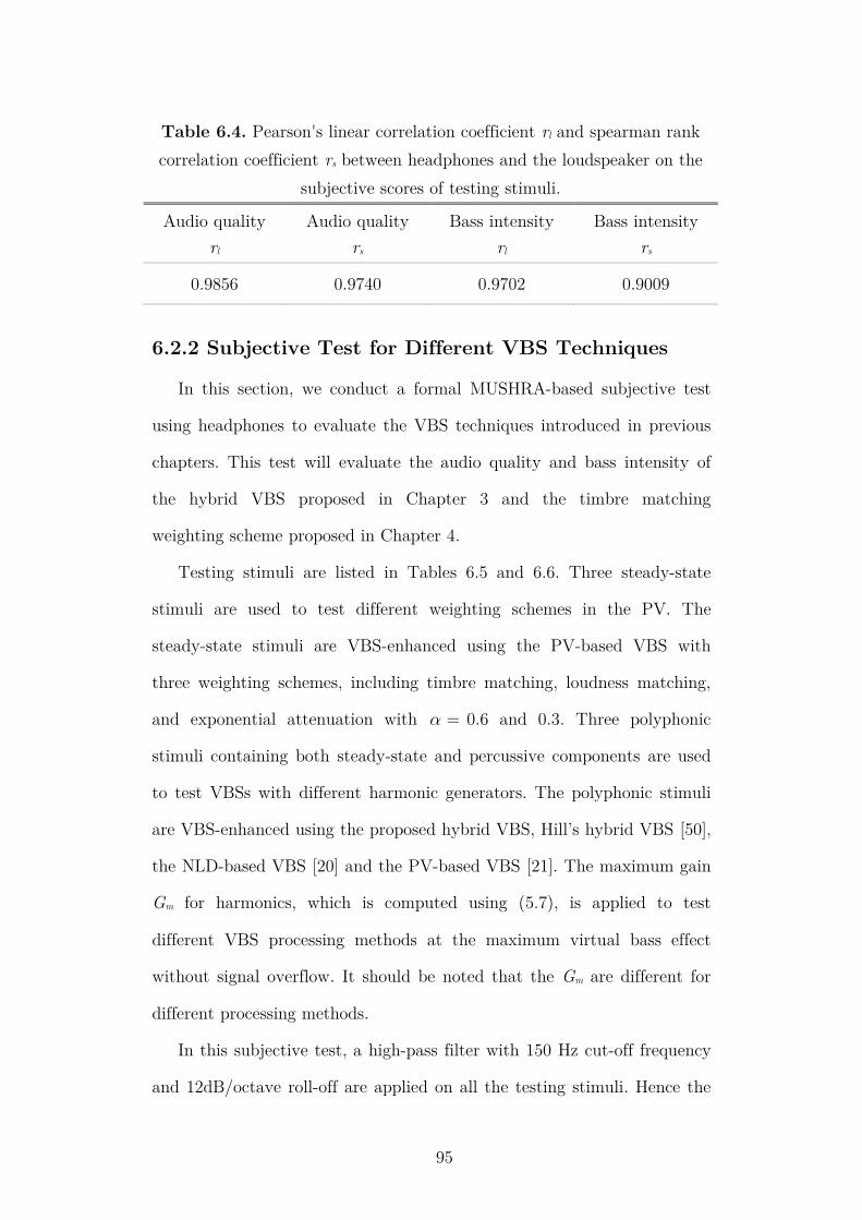
95

6.2.2 Subjective Test for Different VBS Techniques

In this section, we conduct a formal MUSHRA-based subjective test

using headphones to evaluate the VBS techniques introduced in previous

chapters. This test will evaluate the audio quality and bass intensity of

the hybrid VBS proposed in Chapter 3 and the timbre matching

weighting scheme proposed in Chapter 4.

Testing stimuli are listed in Tables 6.5 and 6.6. Three steady-state

stimuli are used to test different weighting schemes in the PV. The

steady-state stimuli are VBS-enhanced using the PV-based VBS with

three weighting schemes, including timbre matching, loudness matching,

and exponential attenuation with α = 0.6 and 0.3. Three polyphonic

stimuli containing both steady-state and percussive components are used

to test VBSs with different harmonic generators. The polyphonic stimuli

are VBS-enhanced using the proposed hybrid VBS, Hill’s hybrid VBS [50],

the NLD-based VBS [20] and the PV-based VBS [21]. The maximum gain

Gm for harmonics, which is computed using (5.7), is applied to test

different VBS processing methods at the maximum virtual bass effect

without signal overflow. It should be noted that the Gm are different for

different processing methods.

In this subjective test, a high-pass filter with 150 Hz cut-off frequency

and 12dB/octave roll-off are applied on all the testing stimuli. Hence the

Table 6.4. Pearson's linear correlation coefficient rl and spearman rank

correlation coefficient rs between headphones and the loudspeaker on the

subjective scores of testing stimuli.

Audio quality

rl

Audio quality

rs

Bass intensity

rl

Bass intensity

rs

0.9856 0.9740 0.9702 0.9009

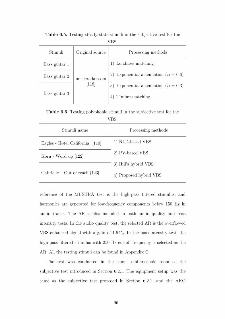
96

reference of the MUSHRA test is the high-pass filtered stimulus, and

harmonics are generated for low-frequency components below 150 Hz in

audio tracks. The AR is also included in both audio quality and bass

intensity tests. In the audio quality test, the selected AR is the overflowed

VBS-enhanced signal with a gain of 1.5Gm. In the bass intensity test, the

high-pass filtered stimulus with 250 Hz cut-off frequency is selected as the

AR. All the testing stimuli can be found in Appendix C.

The test was conducted in the same semi-anechoic room as the

subjective test introduced in Section 6.2.1. The equipment setup was the

same as the subjective test proposed in Section 6.2.1, and the AKG

Table 6.5. Testing steady-state stimuli in the subjective test for the

VBS.

Stimuli Original source Processing methods

Bass guitar 1

musicradar.com [118]

1) Loudness matching

2) Exponential attenuation (α = 0.6)

3) Exponential attenuation (α = 0.3)

4) Timbre matching

Bass guitar 2

Bass guitar 3

Table 6.6. Testing polyphonic stimuli in the subjective test for the

VBS.

Stimuli name Processing methods

Eagles - Hotel California [119] 1) NLD-based VBS

2) PV-based VBS

3) Hill’s hybrid VBS

4) Proposed hybrid VBS

Korn - Word up [122]

Gabrielle – Out of reach [123]

97

K271MKII [115] studio headphones were used for listening. A total of 20

subjects (14 males and 6 females) between 23 to 35 years old participated

in the subjective test. None of the subjects has any history of hearing

disorders. Audio quality was evaluated first and followed by the bass

intensity. The duration was around 20-30 minutes, depending on subjects’

preference to switch between stimuli.

The procedure of the subjective test was the same as the test

introduced in Section 6.2.1. In the training phase, subjects were

introduced to the basic concept of the VBS, and how virtual bass effect

can be generated. Subjects can play all reference and testing stimuli to get

familiar with the VBS effect. In the evaluation pause, subjects can listen

to the stimuli as many times as desired. They were asked to assign scores

of testing stimuli by comparing with the reference stimulus in aspects of

audio quality and bass intensity. The sliders were used to assign the

scores between 0 and 100 units.

After the test, a post-screening was conducted to exclude those

subjects who provided unreliable scores, using the same rule as the

MUSHRA test proposed in Section 6.2.1. In this test, three subjects were

excluded in the audio quality test, and two subjects were excluded in the

bass intensity test. The mean scores of steady-state and polyphonic

stimuli with 95% confidence intervals are shown in Table 6.7 and Table

6.8, respectively.

Table 6.7 shows the performance of different weighting schemes

proposed in Chapter 4. It is found that the proposed timbre matching

weighting scheme outperforms the other three weighting schemes in the

audio quality. Loudness and exponential attenuation with α = 0.3

weighting schemes have the poorest quality (below 30 units). It is also

98

noted that the exponential attenuation scheme with faster attenuation (α

= 0.6) has better audio quality than slower attenuation (α = 0.3). The

objective test in Section 4.2.4 showed that the proposed timbre weighting

scheme can improve the unnatural sharpness effect of the VBS, and

produce more a natural sound than conventional weighting schemes.

Combining with the subjective results, we found that the reduction in

sharpness effect can result in better perceptual quality of steady-state

VBS-enhanced signals. For the bass intensity shown in Table 6.7, all the

weighting schemes are above 70 units with the maximum gain for

harmonics. Loudness and exponential attenuation with α = 0.3 weighting

schemes are a slightly better, but their audio quality are unacceptable.

Results of polyphonic stimuli (in Table 6.8) show the performances of

the VBSs with different harmonic generators proposed in Chapter 3.

Except the PV-based VBS, the audio quality of all the harmonic

generators is in the good grade (60-80). As introduced in Chapter 3, the

proposed hybrid VBS combines NLD and PV, and overcomes the

Table 6.7. Subjective scores for the steady-state stimuli with 95%

confidence interval. (EXA: exponential attenuation, MS: mean scores,

LCB: lower confidence bound, UCB: upper confidence bounds).

Steady-state stimuliAudio quality Bass intensity

LCB MS UCB LCB MS UCB

HRF 94.56 95.55 96.54 49.15 50.10 51.05

Loudness matching 21.58 26.27 30.97 73.81 77.86 81.92

EXA (α = 0.3) 19.61 22.63 25.95 73.95 78.51 83.07

EXA (α = 0.6) 31.67 37.16 42.64 72.14 75.37 78.61

Timbre matching 53.07 59.14 65.20 69.82 72.71 75.59

AR 2.36 4.27 6.19 8.53 11.47 14.41

99

shortcomings of the VBS using the single harmonic generator. Compared

to Hill’s hybrid VBS, the proposed hybrid VBS uses a more effective

separation method for input signals. These advantages of the proposed

hybrid VBS result in the highest audio quality in the subjective test

compared to other harmonic generators. In addition, bass intensity scores

of all the VBSs are above 60 units. The bass intensity of the NLD-based

VBS is the highest, which outperforms the proposed hybrid VBS by 8

units. However, the audio quality of the NLD-based VBS is lower than

the proposed hybrid VBS by 12 unites, which is more than half of the

quality grade.

6.3 Objective Quality Assessment for the VBS

In this section, we first introduce some conventional objective quality

metrics, and evaluate their accuracy of evaluating the perceptual quality

of VBS-enhanced signals by comparing with the subjective scores obtained

in Section 6.2. Subsequently, we propose a new perceptual quality metric

Table 6.8. Subjective scores for the polyphonic stimuli with 95%

confidence interval. (MS: mean scores, LCB: lower confidence bound,

UCB: upper confidence bounds).

Polyphonic stimuliAudio quality Bass intensity

LCB MS UCB LCB MS UCB

HRF 95.16 96.12 97.07 50.47 51.25 52.04

NLD 56.338 62.27 68.17 69.26 72.84 76.43

PV 42.70 49.98 57.26 57.31 62.35 67.40

Hill Hybrid 60.28 65.35 70.43 62.84 66.45 70.06

Proposed Hybrid 69.90 74.94 79.98 60.94 64.71 68.47

AR 30.73 35.67 40.60 10.00 12.51 15.05

100

[122], which has better performance in predicting subjective scores of the

VBS. This work was also published in the IEEE/ACM Transactions on

Audio, Speech, and Language Processing (TASLP) [122].

6.3.1 Objective Evaluation using Conventional Metrics

Earlier studies used some low-level features of audio signals to

objectively assess the audio quality of VBS-enhanced signals, but none of

them utilized modeling of the human auditory system. Oo et al. [17]

analyzed the harmonic richness (HR) of different harmonic generators.

The HR is defined as the root-mean-square (RMS) ratio between

additional harmonics and low-frequency components of VBS-enhanced

signals:

(6.1)

where G is the gain for harmonics, xHA(n) and xLF(n) represent synthesized

harmonics and low-frequency components of the original signal,

respectively.

As introduced in Section 4.2.4, Mu et al. [67] used audio spectrum

centroid (ASC) to compare the perceptual sharpness of VBS-enhanced

signals with different weighting schemes. Due to additional harmonics, the

average frequency of the spectrum is increased, and the VBS-enhanced

signal is usually perceived to be sharper than original signals [2]. ASC

gives the center of gravity of the log-frequency power spectrum, and can

be regarded as an approximation of perceptual sharpness of the signal [70].

Besides these objective metrics, we are also interested in the

performance of the commonly used PEAQ [87] algorithm on VBS-

enhanced signals. The PEAQ incorporates some previously developed

perceptual quality metrics and defines them as model output variables

101

(MOVs). As summarized in Table 6.9, the MOVs quantify different

perceptual features of the audio signal. For example, the MOVs

RmsNoiseLoudB, Total NMRB and RelDistFramesB are related to

distortion loudness or masked distortion level of the processed signal; the

Table 6.9. Model output variables (MOVs) in the PEAQ Basic Mode

(from [84]).

Index MOV Description

1 WinModDiff1BModulation difference with sliding window

average

2 AvgModDiff1BModulation difference with temporally

weighted time average

3 AvgModDiff2B

Modulation difference with temporally

weighted time average and emphasis on

introduced modulations where the reference

contains little or no modulations

4 RmsNoiseLoudBRoot-mean-square of the partial loudness of

noise in the presence of masking.

5 BandwidthRefB Bandwidth of the reference stimulus

6 BandwidthTestB Bandwidth of the testing stimulus

7 Total NMRB Total noise-to-mask ratio

8 RelDistFramesB Relative fraction of disturbed frames

9 MFPDBMaximum filtered probability of detecting the

existence of distortion

10 ADBBAverage distortion steps above the just

noticeable difference

11 EHSB Harmonic structure of the error

102

MOVs WinModDiff1B, AvgModDiff1B and AvgModDiff2B are related to

modulation difference between processed and reference signals; the MOVs

MFPDB and ADBB are related to probability of noise detection in the

processed signal.

The PEAQ estimates the perceptual quality of the audio signal by

mapping the MOVs to a single score, which is called the objective

difference grade (ODG), using neural networks with 1 hidden layer and 3

nodes [123]. It should be noted that the ODG is primarily designed only

for evaluating the quality of digital coded audio signals that are

perceptually lossless, and it is not suitable for highly impaired audio

signals [110].

To evaluate the suitability of HR, ASC and ODG as perceptual

quality metrics for VBS-enhanced signals, we test these metrics on the

stimuli used in the subjective test. A MATLAB implementation of the

PEAQ basic version, which is developed by Kabal [123], is used in our

test. As stimuli in the subjective test are enhanced using different VBS

methods, they are divided into two groups, steady-state (SS) stimuli (in

Table 6.5) and polyphonic (PP) stimuli (in Table 6.6), for the objective

test. More specifically, there are three sets of steady-state bass guitar solo

stimuli, and three sets of polyphonic stimuli containing both steady-state

and percussive components.

The Pearson's linear correlation coefficient rl and the Spearman rank

correlation coefficient rs [121] between objective scores and subjective

scores are computed to determine the predictive performance of these

objective metrics, as shown in Table 6.10. The Pearson's linear correlation

coefficient measures prediction accuracy of objective metrics. On the other

hand, the Spearman rank correlation coefficient measures prediction

103

monotonicity [124], i.e. it measures the correlation of the rank order

between objective and subjective scores for different VBS processing

methods.

As shown in Table 6.10, the HR is poorly correlated with the

subjective scores, which implies that the perceptual audio quality of VBS-

enhanced signals cannot be simply quantified based on the amount of

additional harmonics. The ASC shows better prediction accuracy and

monotonicity for steady-state stimuli, which indicates that the perceptual

sharpness is an important factor for perceptual quality of steady-state

VBS-enhanced signals. This finding confirms our observation on the

relation between the objective results in Section 4.2.4 and the subjective

results in Section 6.2.2. However, performance of the ASC on polyphonic

stimuli is the lowest among the three metrics, and it does not serve well

as an indicator for polyphonic VBS-enhanced signals. The ODG from

PEAQ only show fair prediction accuracy for steady-state stimuli, its

performance on other criteria is unacceptable. This is due to the fact that

the VBS generally leads to high audio impairment. In summary, the

objective metrics HR, ASC and ODG are not suitable indicators to be

used as perceptual quality metrics for VBS-enhanced signals.

Subsequently, we evaluated the predictive accuracy of each individual

Table 6.10. Pearson's linear correlation coefficient rl and spearman rank

correlation coefficient rs between mean subjective scores and HR, ASC

and ODG (SS: steady-state stimuli, PP: polyphonic stimuli).

rl (SS) rs (SS) rl (PP) rs (PP)

HR -0.46 -0.31 -0.61 -0.58

ASC -0.88 -0.73 -0.27 0.10

ODG 0.82 0.55 0.48 0.59

104

MOV in the PEAQ. The 11 MOVs are generated from the stimuli used in

the subjective test. The Pearson's linear correlation coefficient and the

Spearman rank correlation coefficient between each individual MOV and

the subjective scores are summarized in Table 6.11. It is noted that none

of the MOVs exhibits strong correlation (| r | > 0.9) with the subjective

scores from both steady-state and polyphonic stimuli. In other words,

none of the individual MOV is effective in predicting the perceptual

quality of VBS-enhanced signals.

6.3.2 Proposed Perceptual Quality Metrics

In this sub-section, we propose a new perceptual quality metric to

predict the subjective scores for the VBS by investigating various

combinations of the MOVs. Some earlier studies used the same idea in

designing perceptual quality metrics for audio signals with a wide range of

Table 6.11. Pearson's linear correlation coefficient rl and Spearman rank

correlation coefficient rs between mean subjective scores and individual

MOVs. (SS: steady-state stimuli, PM: polyphonic stimuli).

Index MOV rl (SS) rs (SS) rl (PM) rs (PM)

1 WinModDiff1B -0.79 -0.55 -0.69 -0.47

2 AvgModDiff1B -0.81 -0.66 -0.69 -0.46

3 AvgModDiff2B -0.40 -0.26 -0.61 -0.40

4 RmsNoiseLoudB -0.19 -0.06 -0.29 -0.36

5 BandwidthRefB 0.11 0.26 0.28 0.04

6 BandwidthTestB 0.11 0.26 0.28 0.04

7 Total NMRB -0.66 -0.53 -0.50 -0.48

8 RelDistFramesB -0.60 -0.51 -0.03 -0.05

9 MFPDB -0.14 0.21 0.56 0.35

10 ADBB -0.80 -0.66 -0.81 -0.80

11 EHSB 0.14 0.24 -0.10 -0.10

105

impairment. The MOVs were specifically combined to measure the audio

impairment in audio codecs [102], [125], [126] and the audibility of

harmonic distortion in audio systems [127].

The framework of quality metric training and evaluation is shown in

Figure 6.9. In the training phase, mean subjective scores and selected

combinations of MOVs of the training stimuli are sent into a linear

regression model:

(6.2)

where VQA is the RQA (number of training stimuli) × QQA (number of

selected MOVs) matrix, whose elements represent the selected MOVs of

the training stimuli; yQA is a RQA× 1 vector consisting of the mean

subjective scores of the stimuli, and wQA is a QQA× 1 coefficient vector,

which represents the linear weightings for the MOVs. The least-squares

fitting method [128] is used to find wQA:

(6.3)

where the objective function FQA is given by

Linear Regression

Model

yQA = VQAwQA

Subjective scores yQA

Coefficient wQAPredicted scores sQA

Training phase

Evaluation phase

PEAQ

11 MOVs

MOVCombination

SelectedMOVs VQA

PEAQ

11 MOVs

MOVCombination

SelectedMOVs vQA

SubjectiveTest

sQA = wQATvQA

Training stimuli

Evaluation stimulus

Figure 6.9. Framework of the quality metric training using the linear

regression model, and the quality prediction using the trained model.

106

(6.4)

The solution of this minimization problem is given by

(6.5)

where the operators ( )-1 and ( )T represent matrix inverse and matrix

transpose, respectively. In the evaluation phase, the predicted score sQA of

the evaluation stimulus is calculated using the selected MOVs of the

evaluation stimulus and the coefficient vector wQA obtained from the

regression model:

(6.6)

where vQA is a QQA× 1 vector consisting of the selected MOVs of the

evaluation stimulus.

The linear regression model is a simple and efficient way to combine

MOVs. This kind of linear model has been successfully used to generate

objective metrics for highly impaired audio codecs, and it is less

susceptible to over-training [102]. In a survey of audio quality metrics

[110], the model using the liner regression achieves the best performance.

It is noted that the PEAQ used neural networks to train the ODG

score, but we did not choose this method for the following reasons. In the

PEAQ, MOVs are scaled and shifted into the range of [0, 1] before

applying them in neural networks. Baumgarte and Lerch [129] suggested

that MOVs should be truncated to the range of [0, 1], otherwise the

predicted score may substantially increase when the subjective score

decreases. However, the scaling and shifting parameters provided by ITU

BS.1387 are used for audio signals that are not significantly impaired.

Hence, the truncation of MOVs based on these parameters may influence

the accuracy of obtained quality metrics from neural networks. In

addition, it is necessary to decide several parameters in neural networks,

107

like the number of layers and the number of hidden neurons. The optimal

selection of these parameters may require large amount of time and

resources. Therefore, neural networks are not used in our work.

In the training of the linear regression model, three kinds of perceptual

quality metrics are obtained separately by using different stimuli groups:

steady-state (SS), polyphonic (PP) and combined steady-state and

polyphonic stimuli, as listed in Table 6.12. To determine suitable

combinations of MOVs for the three perceptual quality metrics, we adapt

the minimax-optimal method introduced by Creusere et al. [102]. This

method is summarized as follows:

1) Select the stimuli group and the testing combination of MOVs.

2) Within the stimuli group, one stimuli set (including four VBS-

enhanced stimuli for the same original stimulus) is selected as the

evaluation stimuli, and the remaining stimuli are used to train the

linear regression model.

3) Predicted scores of the evaluation stimuli are calculated using the

trained model. The Pearson's linear correlation coefficient and the

root-mean-square error (RMSE) between the predicted and subjective

scores are computed. The RMSE is defined as:

(6.7)

Table 6.12. Three groups of training stimuli. (SS: steady-state stimuli,

PM: polyphonic stimuli).

Stimuli

groupStimuli number

SS 3 (stimuli sets) × 4 (VBS processing methods per set) = 12

PM 3 (stimuli sets) × 4 (VBS processing methods per set) = 12

SS + PM 6 (stimuli sets) × 4 (VBS processing methods per set) = 24

108

where 𝑦𝑄𝐴

𝑗𝑠𝑡 and 𝑠𝑄𝐴

𝑗𝑠𝑡 are the subjective and predicted scores for the

four evaluation stimuli, respectively.

4) Repeat steps 2) and 3) until all stimuli sets in the group are used as

the evaluation stimuli. The minimum value of the correlation

coefficients and the maximum value of the RMSEs are defined as the

minimum correlation coefficient (MinCorr) and the maximum RMSE

(MaxRMSE) for the selected combination of MOVs and the stimuli

group, respectively.

The MinCorr and MaxRMSE estimate the worst predictive accuracy of

the selected combinations of MOVs. All the possible combinations of

MOVs are tested for the three stimuli groups, and the combinations of

MOVs having maximum MinCorr and minimum MaxRMSE, as well as

the combination of all 11 MOVs are summarized in Tables 6.13-6.15.

As listed in Table 6.13-Table 6.15, the perceptual quality metrics using

all 11 MOVs lead to low MinCorrs and high MaxRMSEs, which implies

that the trainings are over-fitted. Predicted scores from the metrics based

on the listed combinations of MOVs are all highly correlated with the

subjective scores (MinCorr > 0.9). None of the combinations of MOVs has

a MaxRMSE larger than 10 units. The metrics with combinations of

MOVs {2, 4, 7, 8}, {1, 2, 7, 9, 10} and {5, 6, 7, 9, 10} produce the most

accurate prediction for separate groups of steady-state and polyphonic

stimuli, and combined steady-state and polyphonic stimuli, respectively.

As introduced in Section 6.2, the quality grades (e.g., Poor, Fair, Good,

etc.) are separated every 20 units in the subjective test. Therefore, the

average predictive errors from all of the listed metrics are below half

quality grade. These results indicate the high accuracy of the perceptual

quality metrics using the listed combinations of MOVs.

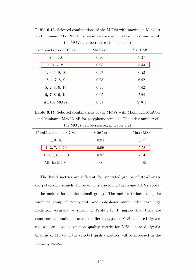
109

The listed metrics are different for separated groups of steady-state

and polyphonic stimuli. However, it is also found that some MOVs appear

in the metrics for all the stimuli groups. The metrics trained using the

combined group of steady-state and polyphonic stimuli also have high

prediction accuracy, as shown in Table 6.15. It implies that there are

some common audio features for different types of VBS-enhanced signals,

and we can have a common quality metric for VBS-enhanced signals.

Analysis of MOVs in the selected quality metrics will be proposed in the

following section.

Table 6.13. Selected combinations of the MOVs with maximum MinCorr

and minimum MaxRMSE for steady-state stimuli. (The index number of

the MOVs can be referred in Table 6.9)

Combinations of MOVs MinCorr MaxRMSE

7, 9, 10 0.96 7.27

2, 4, 7, 8 0.98 5.43

1, 3, 4, 9, 10 0.97 6.52

2, 4, 7, 8, 9 0.98 6.62

5, 7, 8, 9, 10 0.95 7.62

6, 7, 8, 9, 10 0.95 7.64

All the MOVs 0.51 278.4

Table 6.14. Selected combinations of the MOVs with Maximum MinCorr

and Minimum MaxRMSE for polyphonic stimuli. (The index number of



4, 9, 10 0.94 5.97

1, 2, 7, 9, 10 0.99 5.78

1, 2, 7, 8, 9, 10 0.97 7.84

All the MOVs -0.84 60.29

110

6.4 Analysis of Quality Metrics

From the objective test in the Section 6.3.2, we found several metrics

that are accuracy for predicting the perceptual quality of VBS-enhanced

signals. A simple inspection of Table 6.13-6.15 reveals that some MOVs,

like 7, 9 and 10, are retained in most the listed metrics. To analyze the

significance of these MOVs, we perform the ANOVA test on the selected

quality metrics:

(6.8)

where H0 is the null-hypothesis, Ha is the alternative-hypothesis, and q

QAw

is the coefficient for the qth MOV. This null-hypothesis implies that the

metric’s predictive capability is not reduced by removing the qth MOV.

The ANOVA test provides a p-value for each MOV. A low p-value (<

0.05) indicates that the null hypothesis is rejected (at 5% significance

level), and the corresponding MOV is a significant term in the metric. In

Table 6.15. Selected combinations of the MOVs with maximum MinCorr

and minimum MaxRMSE for combined steady-state and polyphonic

stimuli. (The index number of the MOVs can be referred in Table 6.9)


5, 7, 9, 10 0.95 5.91

6, 7, 9, 10 0.95 5.91

5, 6, 7, 9, 10 0.95 5.83

5, 7, 8, 9, 10 0.95 5.93

5, 7, 9, 10, 11 0.91 5.96

6, 7, 8, 9, 10 0.91 5.93

6, 7, 9, 10, 11 0.95 5.97

All the MOVs 0.50 12.54

111

contrast, a high p-value indicates that the corresponding MOV is a non-

significant term of the metric.

Different from the minimax-optimal method in Section 6.3, we use all

the stimuli sets within the group to train the metric and compute the p-

value for each MOV in the metric. The result is shown in Table 6.16-

Table 6.18. We found that the MOVs 7 (Total NMRB), 9 (MFPDB) and

Table 6.16. ANOVA p-values for the MOVs from the derived perceptual

quality metrics for steady-state stimuli (in Table 6.13).

MOVs 7 9 10

p-value 0.000 0.000 0.000

MOVs 2 4 7 8

p-value 0.000 0.000 0.000 0.000

MOVs 1 3 4 9 10

p-value 0.018 0.032 0.003 0.000 0.000

MOVs 2 4 7 8 9

p-value 0.000 0.000 0.000 0.134 0.484

MOVs 5 7 8 9 10

p-value 0.451 0.004 0.404 0.023 0.000

MOVs 6 7 8 9 10

p-value 0.447 0.004 0.401 0.023 0.000


quality metrics for polyphonic stimuli (in Table 6.14).

MOVs 4 9 10

p-value 0.050 0.000 0.000

MOVs 1 2 7 9 10

p-value 0.031 0.031 0.003 0.000 0.000

MOVs 1 2 7 8 9 10

p-value 0.031 0.032 0.003 0.000 0.000 0.000

112

10 (ADBB) give consistently small p-values in all the perceptual quality

metrics, which indicates their significance in these metrics. Hence, the

MOVs Total NMRB, MFPDB and ADBB can capture the most important

audio features on the perceptual quality of VBS-enhanced signals.

Total NMRB estimates the audible noise energy of the stimulus by

measuring the noise-to-mask ratio (NMR). The noise signal is determined

as the difference between the magnitude spectra of reference and

processed stimuli, and the masking threshold is given by the reference

stimulus. In PEAQ, Total NMRB of the entire stimulus is the temporal

linear average of the instantaneous NMRs that are calculated over 2048-

sample frames with 50% overlapping across the stimulus. Figure 6.10


quality metrics for combined steady-state and polyphonic stimuli (in

Table 6.15).

MOVs 5 7 9 10

p-value 0.000 0.000 0.000 0.000

MOVs 6 7 9 10

p-value 0.000 0.000 0.000 0.000

MOVs 5 6 7 9 10

p-value 0.392 0.396 0.000 0.000 0.000

MOVs 5 7 8 9 10

p-value 0.000 0.000 0.727 0.000 0.000

MOVs 5 7 9 10 11

p-value 0.000 0.000 0.000 0.000 0.300

MOVs 6 7 8 9 10

p-value 0.000 0.000 0.729 0.000 0.000

MOVs 6 7 9 10 11

p-value 0.000 0.000 0.000 0.000 0.300

113

shows an example of the instantaneous NMRs across a steady-state VBS-

enhanced stimulus used in the subjective test with different weighting

schemes. In this example, timbre matching achieves the lowest Total

NMRB, while loudness matching and exponential attenuation with α = 0.3

exhibit the highest values. This ranking of Total NMRB from different

weighting schemes matches the subjective results shown in Table 6.7.

The MOV ADBB and MFPDB are based on the probability of noise

detection, which is derived by comparing the excitation difference between

reference and processed stimuli to the just noticeable difference (JND)

[130]. The MOV MFPDB is the maximum value of smoothed version of

probability of noise detection:

0 0.5 1 1.5 2 2.5 3-40

-30

-20

-10

0

10

20

0 0.5 1 1.5 2 2.5 3-1

-0.5

0

0.5

1

Loudness = 7.37Exp(0.3) = 7.92Exp(0.6) = 3.46Timbre = -2.81

Total NMRB

(b)

(a)

Time (sec)

inst

anta

neo

us

NM

R (

dB

)A

mplitu

de

Figure 6.10. (a) Plot of the reference steady-state stimulus. (b)

Instantaneous NMRs of the VBS-enhanced stimuli with different

weighting schemes. The legend shows the MOV Total NMRB of the

stimuli.

114

(6.9)

where PDE(m) represents the probability of noise detection in the frame m,

c0 and c1 are constants, mend is the last frame of the stimulus. The MOV

ADBB is calculated by averaging the total distortion steps above the

threshold:

(6.10)

where mDE represents the frames with the probability of noise detection

PDE(m) exceeding a threshold of 0.5, and QDE(m) represents distortion

steps above the threshold in one frame.

From the studies on the significant MOVs in the quality metrics, we

found that the perceptual quality of VBS-enhanced signals is highly

dependent on the level of perceptual noise. It should be noted that,

although these MOVs are significant in the derived metrics, they cannot

be individually used as the perceptual quality metric. As mentioned in

Table 6.11, none of the individual MOV exhibits strong correlation with

the subjective scores, but perceptual noise that quantified by the MOVs

Total NMRB and ADBB are highly related to the perceptual quality of

VBS-enhanced signals.

However, only steady-state and polyphonic stimuli were used in the

test. We are also interested in the significant MOVs for pure percussive

VBS-enhanced signals, because the important audio features related to the

115

perceptual quality for pure percussive VBS-enhanced signals may help us

to improve NLD harmonic generators.

Hence, another MUSHRA-based subjective test was conducted using

the four sets of VBS-enhanced percussive stimuli. All stimuli are repeating

bass drum sound from Roland TR-626 sound library [62], and plots of the

stimuli are shown in Figure. 6.11. The procedure of the subjective test

was the same as the test introduced in Section 6.2.2, and 20 subjects (15

males and 5 females) participated in the subjective test.

After the test, the subjective result and MOVs were used to train the

quality metric in the linear regression model. The minimax-optimal

method was used to select the combinations of MOVs having maximum

MinCorr and minimum MaxRMSE. The selected combinations of MOVs

are listed in Table 6.19. Predicted scores from the quality metrics based

on the listed combinations of MOVs are all highly correlated with the

subjective scores (MinCorr > 0.9). None of the combinations of MOVs has

a MaxRMSE larger than 10 units.

Subsequently, the ANOVA test was performed on the quality metrics

for percussive stimuli, and the result is shown in Table 6.20. We found

0 0.5 1 1.5 2 2.5 3-1

-0.5

0

0.5

1(a)

0 0.5 1 1.5 2 2.5 3-1

-0.5

0

0.5

1(b)

(c) (d)

0 0.5 1 1.5 2-1

-0.5

0

0.5

1

0 0.5 1 1.5 2 2.5-1

-0.5

0

0.5

1

Time (Sec) Time (Sec)

Am

plitu

de

Time (Sec) Time (Sec)

Am

plitu

de

Figure 6.11. Plots of the testing percussive stimuli.

116

that the MOV 7 (Total NMRB), 9 (MFPDB) and 10 (ADBB) also show

significance in some metrics. However, the most significant MOV for

percussive stimuli is the MOV 1 (WinModDiff1B).

The MOV WinModDiff1B is related to modulation difference

(ModDiff), which measures the changes of temporal envelopes between the

processed and reference signals. WinModDiff1B is calculated by windowed

averaging the instantaneous ModDiff across the stimulus. The

instantaneous ModDiff is the absolute difference between the local

modulation measures of the reference and testing stimuli, normalized by

the local modulation measure of the reference stimulus:

(6.11)

Table 6.19. Selected combinations of the MOVs with Maximum MinCorr

and Minimum MaxRMSE for percussive stimuli. (The index number of



1, 7, 10 0.98 5.45

1, 8, 9 0.97 7.62

1, 4, 8, 9 0.96 5.89

1, 8, 9, 10 0.96 6.96


quality metrics for percussive stimuli (in Table 6.19).

MOVs 1 7 10

p-value 0.000 0.000 0.003

MOVs 1 8 9

p-value 0.000 0.101 0.000

MOVs 1 4 8 9

p-value 0.000 0.963 0.223 0.000

MOVs 1 8 9 10

p-value 0.000 0.265 0.002 0.583

117

where m and k represent the frame and frequency indices, respectively;

ModT(m,k) and ModR(m,k) are the local modulation measure of testing

and reference stimuli, respectively; Nc represent the number of frequency

bands. Figure 6.12 shows an example of the instantaneous ModDiff curve

of VBS-enhanced percussive stimuli with different gain for harmonics. The

maximum gain Gm for harmonics without signal overflow is computed

according to (5.7). The other gains are set as 0.5Gm and 0.25Gm. An

overflowed VBS-enhanced signal with a gain of 1.5Gm is also included.

The lower gain for harmonics results in lower instantaneous ModDiff and

WinModDiff1B, which matches our observation in the subjective test

proposed in Section 6.2.1. It is also found that temporal envelope changes

in the percussive stimuli mostly occur at decay portions of the drum beats.

0 0.5 1 1.5 2 2.5 3-30

-20

-10

0

10

20

0 0.5 1 1.5 2 2.5 3-1

-0.5

0

0.5

1

0.25GM = 5.40.5GM = 8.11GM = 11.441.5GM = 16.58

(b)

(a)

Am

plitu

de

Inst

anta

neo

us

Mod

Diff (%

)

Time (sec)

Time (sec)

WinModDiff1B

Figure 6.12. (a) Plot of the reference percussive stimulus. (b)

Instantaneous ModDiff of the VBS-enhanced stimuli with different gains

for harmonics. The legend shows the MOV WinModDiff1B of the stimuli.

118

Only the overflowed stimulus has a significant peak of instantaneous

ModDiff at the percussive period. This is because the clipping distortion

at these periods heavily distorts temporal envelopes of the stimulus.

6.5 Chapter Summary

In this chapter, we first carried out subjective test based on the

MUSHRA to assess the VBS techniques proposed in previous chapters,

and the testing results revealed advantages of the proposed techniques.

The perceptual quality of the hybrid VBS proposed in Chapter 3 was

around 12 and 25 units higher than using the single NLD and the single

PV harmonic generator in a 0-100 scale, respectively. The timbre

matching scheme proposed in Chapter 4 improved the perceptual quality

of VBS-enhanced signals by 22 to 37 units compared to other weighting

schemes. The overflowed signal that was used as the anchor received

unacceptable subjective scores, which justify the need of including an

overflow control mechanism in the VBS.

Subsequently, we developed an objective perceptual quality metric

based on MOVs of the PEAQ to predict perceptual quality of VBS-

enhance signals. Compared to the time-consuming subjective test, the

objective metric provides a more convenient way of quality assessment.

Perceptual quality metrics were derived by training a linear regression

model with subjective scores and selected combinations of MOVs of VBS-

enhanced signals. Suitable combinations of MOVs were obtained from the

perceptual quality metrics that are most correlated to the subjective

scores. The proposed test revealed that the derived perceptual quality

metrics have high prediction accuracy for both steady-state and

polyphonic stimuli. In contrast, previous objective metrics for the VBS,

119

which do not use psychoacoustic modelling, show poor correlation with

subjective scores.

Our studies also showed that the MOVs Total NMRB, MFPDB and

ADBB are important in determining the perceptual quality metrics for

different types of VBS-enhanced signals. By analyzing the meaning of

these MOVs, we found that the perceptual noise is significantly relevant

to the perceptual quality of VBS-enhanced signals. In addition, the MOV

WinModDiff1B, which describes the temporal envelope change of signals, is

found to be the most important in determining the perceptual quality

metrics for percussive VBS-enhanced signals.

120

Conclusions and Future Works

7.1 Conclusions

In this thesis, a virtual bass system (VBS) was proposed to improve

the bass performance for small loudspeakers that cannot reproduce low

frequencies due to size limitation. The VBS is based on a psychoacoustic

phenomenon, called missing fundamental effect. Suitably synthesized

harmonics are injected to the audio signal to produce perception of bass

components that are lower than the loudspeaker’s cut-off frequency. The

VBS is more effective compared to the conventional low-frequency

amplification method, which usually leads to distortion and possibly

overloads the loudspeaker when high amplification is applied. However,

due to additional harmonics, the VBS may also produce perceivable

distortion and reduce the perceptual quality of the original signal. Thus,

this thesis proposed three techniques of improving the audio quality of the

VBS and an objective metric that provides a convenient approach to

assess the perceptual quality of VBS-enhanced signals.

The harmonic generator plays a key role in the VBS. Previous

harmonic generators, namely the nonlinear device (NLD) and the phase

vocoder (PV), have their own unique advantages and drawbacks. The

NLD and the PV were found to be more suitable for percussive and

steady-state signals, respectively. Hence, a hybrid VBS was proposed in

Chapter 3. The hybrid VBS separates the input signal into percussive and

121

steady-state components using a median filter based method, and uses

different approaches to generate harmonics. In the subjective test with

five quality grades (Bad, Poor, Fair, Good and Excellent), the proposed

hybrid VBS can improve the perceptual quality by more than half to one

quality grade, compared to the VBS with a single harmonic generator. In

addition, the objective testing results showed that the proposed separation

method was much more effective compared to the method that was

previously used in the VBS.

In Chapter 4, two techniques were proposed to improve the quality of

the PV in the hybrid VBS. An improved PV synthesis approach with

phase coherence maintaining techniques was proposed. Compared to the

conventional PV used in the VBS, the proposed PV had lesser spectral

distortions. In addition, a new timbre matching scheme for harmonic

weighting was designed to preserve the timbre of the original signal in the

VBS-enhanced signal. The spectral envelope of the original signal, which

was highly related to the timbre, was maintained in the VBS-enhanced

signal. The objective test indicated that the proposed timbre weighting

scheme can more effectively reduce the unnatural sharpness effect caused

by additional harmonics compared to conventional weighting schemes. In

the subjective test, the timbre weighting scheme improved the perceptual

quality of VBS-enhanced signals by more than one quality grade. In

addition, the objective analysis indicated that the sharpness effect was

highly correlated to the perceptual quality of steady-state VBS-enhanced

signals.

Mixing of additional harmonics and original signals may cause

arithmetic overflow and clipping distortion in the VBS-enhanced signal,

especially for high-level percussive components. In the subjective test, all

122

the overflowed VBS-enhanced signals are graded as “Poor” or “Bad”

quality. Therefore, Chapter 5 proposed a harmonic gain control method to

prevent signal overflow in the VBS. A detection method of percussive

events was designed, and a suitable gain limit for additional harmonics

was computed for each percussive event. The evaluation results indicated

that the proposed method can effectively prevent signal overflow in the

VBS. Compared to the commonly used limiter method, the proposed gain

control method does not require any parameter adjustment for different

types of audio tracks, and has no influence on the high-frequency

components of the original signal. The system delay caused by the

proposed method was short enough (122 ms to 174 ms) for real-time video

and audio applications.

In Chapter 6, an objective perceptual quality metric for the VBS was

proposed. Compared to the time-consuming subjective test, the objective

metric provides a convenient approach to evaluate the perceptual quality

of VBS-enhanced signals. The proposed perceptual quality metrics were

built based on the model output variables (MOVs) of the commonly used

PEAQ (Perceptual Evaluation of Audio Quality) algorithm. The MOVs

applied a model of human auditory system to represent different features

related to the perceptual audio quality. Our test revealed that the derived

perceptual quality metrics were accurate for both steady-state and

polyphonic stimuli (correlation>0.95). On the other hand, some

conventional objective quality metrics for the VBS and the PEAQ showed

poor correlation (correlation<0.8) with subjective scores for either steady-

state or polyphonic stimuli. Hence, the proposed objective metric provides

a convenient and accurate way to assess the perceptual quality of VBS-

enhanced signals and to compare different processing approaches in the

123

design of the VBS. By analyzing the proposed objective metrics, we found

that the MOVs describing the perceptual noise are significantly relevant

to the perceptual quality of all types of VBS-enhanced signals. In addition,

the MOV describing the temporal envelope change was found to be the

most important in determining the perceptual quality metrics for

percussive VBS-enhanced signals.

7.2 Future works

Through the improved VBS techniques reported in this thesis, several

interesting extensions are worthy to be explored in the future. In Chapter

6, it was found that the temporal envelope change of signals is important

in determining the perceptual quality metrics for percussive VBS-

enhanced signals. This finding provides a new basis to improve the VBS.

In our VBS research, the timbre technique based on spectral envelope

matching has been established for the PV, and we can also carry out the

research on temporal envelope matching for percussive harmonics

generated by the NLD.

In addition, the current VBS still requires users to manually determine

the gain for harmonics. However, a fixed gain for harmonics may not be

suitable for different types of stimuli. Hence, when playing different types

of audio tracks, for example, from hip-hop to classical, users have to

manually change the gain in the VBS, which is very inconvenient.

Therefore, an automatic gain adjustment technique can be used to

adaptively determine the gain for harmonics to achieve the best audio

quality based on audio features of the input signal. This adaptive gain

algorithm can also be combined with the overflow control method

proposed in Chapter 5. To determine the gain for harmonics that is most

124

suitable for majority subjects, it is necessary to build a large subjective

database with different types of stimuli. Subjects should be asked to

choose the most suitable gain they prefer. Subsequently, the audio

features that are most correlated to majority of subjects’ preference for

the gain of harmonics can be determined. Audio features, such as ratio

between the energy of low-frequency components and high-frequency

components, the dominant types of bass (steady-state or percussive), and

the tempo of the stimuli, are potentially related to the suitable gain in the

VBS. Finally, a model that maps the audio features to the most suitable

gain is built by training the subjective results and audio features. The

gain for the new signal is determined by sending their audio features into

the model.

Next, the proposed objective model can only assess the perceptual

quality of VBS-enhanced signals. A reliable model that can predict the

bass intensity based on subjective preference is valuable for the VBS

research. To the author’s knowledge, there is no study on the objective

(perceptual) prediction for the bass intensity of VBS-enhanced signals.

The bass intensity metric and the proposed perceptual quality metric may

also help in the construction of the automatic gain adaption system for

the VBS. However, this research is related to the missing fundamental

effect, and may require a comprehensive study into the psychoacoustics.

Currently, a real-time VBS application based on MATLAB GUI has

been implemented. More details about the application are introduced in

Appendix B. However, due to high computational demands from the

proposed VBS techniques, the un-optimized MATLAB code results in

high CPU utilization and memory usage. An optimized version of the

VBS can be more efficiently programmed in C or Java and run in iOS or

125

Android for portable devices.

126

Author’s Publication

[A.1] H. Mu, W. S. Gan, and E. L. Tan, “An Objective Analysis Method

for Perceptual Quality of a Virtual Bass System,” Audio, Speech,

and Language Processing, IEEE/ACM Transactions on, vol. 23, no.

5, pp. 840–850, 2015.+

[A.2] H. Mu and W. S. Gan “Perceptual Quality Improvement for

Virtual Bass System,” Journal of the Audio Engineering Society,

2015 [Accepted].

[A.3] H. Mu, W. S. Gan, and E. L. Tan, “A psychoacoustic bass

enhancement system with improved transient and steady-state

performance,” in Proc. IEEE Int. Conf. Acoustics, Speech and

Signal Processing (ICASSP), Kyoto, Japan, 2012, pp. 141 –144.

[A.4] C. Shi, H. Mu, and W. S. Gan, “A psychoacoustical preprocessing

technique for virtual bass enhancement of the parametric

loudspeaker,” in Proc. IEEE Int. Conf. Acoustics, Speech and

Signal Processing (ICASSP), Vancouver, Canada, 2013, pp. 31–35.

[A.5] H. Mu, W. S. Gan, and E. L. Tan, “A timbre matching approach

to enhance audio quality of psychoacoustic bass enhancement

system,” in Proc. IEEE Int. Conf. Acoustics, Speech and Signal

Processing (ICASSP), Vancouver, Canada, 2013, pp. 36–40.

[A.6] H. Mu and W.-S. Gan, “A virtual bass system with improved

overflow control,” in Proc. IEEE Int. Conf. Acoustics, Speech and

Signal Processing (ICASSP), South Brisbane, Australia, 2015, pp.

1841–1845.

127

References

[1] B. Owsinski, The Mixing Engineer’s Handbook, 2nd ed. Thomson

Course Technology, 2006.

[2] E. R. Larsen and R. M. Aarts, Audio bandwidth extension:

application of psychoacoustics, signal processing and loudspeaker

design. Wiley, 2004.

[3] W. S. Gan, S. M. Kuo, and C. W. Toh, “Virtual bass for home

entertainment, multimedia PC, game station and portable audio

systems,” IEEE Transactions on Consumer Electronics, vol. 47, no.

4, pp. 787–796, 2001.

[4] M. Shashoua and D. Glotter, “Method and system for enhancing

quality of sound signal,” U.S. Patent, 5 930 373, Jul-1999.

[5] D. Ben-Tzur and M. Colloms, “The effect of MaxxBass

psychoacoustic bass enhancement on loudspeaker design,”

presented at the 106th Audio Eng. Soc. Conv., Munich, Germany,

1999.

[6] G. F. M. D. Poortere, C. M. Polisset, and R. M. Aarts, “Ultra

bass,” U.S. Patent, 613 433 017, Oct-2000.

[7] J. F. Schouten, R. J. Ritsma, and B. L. Cardozo, “Pitch of the

residue,” Journal of the Audio Engineering Society, vol. 34, no. 9B,

pp. 1418–1424, 1962.

[8] E. Terhardt, “Calculating virtual pitch,” Hearing Research, vol. 1,

no. 2, pp. 155–182, Mar. 1979.

[9] C. W. Toh and W. S. Gan, “A Real-Time Virtual Surround Sound

System with Bass Enhancement,” in 107th Convention of the

Audio Engineering Society, New York, USA, 1999.

[10] S. E. Tan, W. S. Gan, C. W. Toh, and J. Yang, “Application of

virtual bass in audio crosstalk cancellation,” Electronics Letters,

vol. 36, no. 17, pp. 1500 –1501, Aug. 2000.

[11] W. S. Gan and S. M. Kuo, “Integration of virtual bass

reproduction in active noise control headsets,” in 7th International

Conference on Signal Processing (ICSP ’04), 2004, vol. 1, pp. 368

– 371 vol.1.

128

[12] F. A. Karnapi, Y. H. Liew, K. Lee, and W. S. Gan, “Method to

Enhance Low Frequency Perception from a Parametric Array

Loudspeaker,” 112th Convention of the Audio Engineering Society,

vol. 110, no. 5, p. 2741, 2002.

[13] C. Shi, H. Mu, and W. S. Gan, “A psychoacoustical preprocessing

technique for virtual bass enhancement of the parametric

loudspeaker,” in Proc. IEEE Int. Conf. Acoustics, Speech and

Signal Processing (ICASSP), Vancouver, Canada, 2013, pp. 31–35.

[14] H. Behrends, W. Bradinal, and C. Heinsberger, “Loudspeaker

Systems for Flat Television Sets,” in 123rd Convention of the

Audio Engineering Society, New York, USA, 2007.

[15] B. Pueo, G. Ramos, and J. J. Lopez, “Strategies for bass

enhancement in Multiactuator Panels for Wave Field Synthesis,”

Applied Acoustics, vol. 71, no. 8, pp. 722–730, 2010.

[16] A. J. Hill and M. O. J. Hawksford, “Wide-area psychoacoustic

correction for problematic room modes using non-linear bass

synthesis,” Journal of the Audio Engineering Society, 2012.

[17] N. Oo and W. S. Gan, “Harmonic and intermodulation analysis of

nonlinear devices used in virtual bass systems,” presented at the

124th Audio Eng. Soc. Conv., Amsterdam, Netherlands, 2008.

[18] N. Oo and W. S. Gan, “Analytical and perceptual evaluation of

nonlinear devices for virtual bass system,” in 128th Convention of

the Audio Engineering Society. London, UK, 2010.

[19] N. Oo, W. S. Gan, and W. T. Lim, “Generalized harmonic analysis

of Arc-Tangent Square Root (ATSR) nonlinear device for virtual

bass system,” in 35th IEEE International Conference on Acoustics,

Speech and Signal Processing (ICASSP), 2010, pp. 301–304.

[20] N. Oo, W. S. Gan, and M. O. J. Hawksford, “Perceptually-

Motivated Objective Grading of Nonlinear Processing in Virtual-

Bass Systems,” Journal of the Audio Engineering Society, vol. 59,

no. 11, pp. 804–824, 2011.

[21] M. R. Bai and W. Lin, “Synthesis and Implementation of Virtual

Bass System with a Phase-Vocoder Approach,” Journal of the

Audio Engineering Society, vol. 54, no. 11, pp. 1077–1091, 2006.

[22] D. M. Howard and J. Angus, Acoustics and psychoacoustics.

Taylor & Francis, 2009.

129

[23] G. S. Ohm, “Über die Definition des Tones, nebst daran geknüpfter

Theorie der Sirene und ähnlicher tonbildender Vorrichtungen,”

Annalen der Physik, vol. 135, no. 8, pp. 513–565, 1843.

[24] A. Seebeck, “Beobachtungen über einige Bedingungen der

Entstehung von Tönen,” Annalen der Physik, vol. 129, no. 7, pp.

417–436, 1841.

[25] A. Seebeck, “Ueber die sirene,” Annalen der Physik, vol. 136, no.

12, pp. 449–481, 1843.

[26] H. Von Helmholtz, die Lehre von den Tonempfindungen. Friedrich

Vieweg und Soyhn, 1863.

[27] J. F. Schouten, “The perception of subjective tones,” Proceedings

of the Koninklijke Nederlandse Akademie van Wetenschappen, vol.

41, pp. 1086–1093, 1938.

[28] J. F. Schouten, “The residue and the mechanism of hearing,” in

Proceedings of the Koninklijke. Nederlandse Akademie van

Wetenschappen, 1940, vol. 43, pp. 991–999.

[29] J. Schouten, The residue, a new component in subjective sound

analysis. 1940.

[30] J. Licklider, “‘Periodicity’ pitch and ‘place’ pitch,” The Journal of

the Acoustical Society of America, vol. 26, no. 5, pp. 945–945, 1954.

[31] J. Licklider, “Auditory frequency analysis,” Information theory, pp.

253–268, 1956.

[32] H. M. Jackson and B. C. Moore, “The dominant region for the

pitch of complex tones with low fundamental frequencies,” The

Journal of the Acoustical Society of America, vol. 134, no. 2, pp.

1193–1204, 2013.

[33] R. Plomp, “Pitch of complex tones,” The Journal of the Acoustical

Society of America, vol. 41, no. 6, pp. 1526–1533, 1967.

[34] R. J. Ritsma, “Frequencies dominant in the perception of the pitch

of complex sounds,” The Journal of the Acoustical Society of

America, vol. 42, no. 1, pp. 191–198, 1967.

[35] B. C. Moore, B. R. Glasberg, and R. W. Peters, “Relative

dominance of individual partials in determining the pitch of

complex tones,” The Journal of the Acoustical Society of America,

vol. 77, no. 5, pp. 1853–1860, 1985.

130

[36] H. Dai, “On the relative influence of individual harmonics on pitch

judgment,” The Journal of the Acoustical Society of America, vol.

107, no. 2, pp. 953–959, 2000.

[37] M. F. McKinney and J. Breebaart, “Features for audio and music

classification,” in Proc. ISMIR, 2003, vol. 3, pp. 151–158.

[38] E. R. Larsen and R. M. Aarts, “Reproducing low-pitched signals

through small loudspeakers,” Journal of the Audio Engineering

Society, vol. 50, no. 3, pp. 147–164, 2002.

[39] M. Arora, H. Moon, and S. Jang, “Low Complexity Virtual Bass

Enhancement Algorithm for Portable Multimedia Device,” in 29th

AES International Conference, Seoul, Korea, 2006.

[40] L. K. Chiu, D. V. Anderson, and B. Hoomes, “Audio output

enhancement algorithms for piezoelectric loudspeakers,” in IEEE

Signal Processing Society 14th DSP Workshop & 6th SPE

Workshop, Sedona, Arizona, 2011, pp. 317–320.

[41] F. Nagel, S. Disch, and N. Rettelbach, “A phase vocoder driven

bandwidth extension method with novel transient handling for

audio codecs,” in 127th Conference of the Audio Engineering

Society. Munich, Germany, 2009.

[42] S. Zhang, L. Xie, Z.-H. Fu, and Y. Yuan, “A hybrid virtual bass

system with improved phase vocoder and high efficiency,” in

Chinese Spoken Language Processing (ISCSLP), 2014 9th

International Symposium on, 2014, pp. 401–405.

[43] U. Zö lzer, Digital Audio Signal Processing. John Wiley & Sons,

Ltd, 2008.

[44] J. L. Flanagan and R. M. Golden, “Phase vocoder,” Bell System

Technical Journal, vol. 45, no. 9, pp. 1493–1509, 1966.

[45] D. Griffin and J. Lim, “Signal estimation from modified short-time

Fourier transform,” IEEE Transactions on Acoustics, Speech, &

Signal Processing, vol. 32, no. 2, pp. 236–243, 1984.

[46] J. Laroche and M. Dolson, “New phase-vocoder techniques for

pitch-shifting, harmonizing and other exotic effects,” in

Applications of Signal Processing to Audio and Acoustics, 1999

IEEE Workshop on, 1999, pp. 91–94.

[47] J. Laroche and M. Dolson, “Improved phase vocoder time-scale

modification of audio,” IEEE Transactions on Speech and Audio

Processing, vol. 7, no. 3, pp. 323–332, May 1999.

131

[48] D. D. Greenwood, “Auditory Masking and the Critical Band,” The

Journal of the Acoustical Society of America, vol. 33, no. 4, pp.

484–502, 1961.

[49] C. T. Tan, N. Zacharov, and V. V. Mattila, “Predicting the

Perceived Quality of Nonlinearly Distorted Music and Speech

Signals,” Journal of the Audio Engineering Society, vol. 52, no. 7/8,

pp. 699–711, 2004.

[50] A. J. Hill and M. O. J. Hawksford, “A hybrid virtual bass system

for optimized steady-state and transient performance,” in Proc.

2nd Computer Sci. and Electronic Eng. Conf. (CEEC), Colchester,

UK, 2010, pp. 1,6, 8–9.

[51] U. Zö lzer and X. Amatriain, DAFX: digital audio effects. John

Wiley and Sons, 2002.

[52] R. E. Crochiere and L. R. Rabiner, Multirate digital signal

processing. Prentice-Hall, 1983.

[53] C. Schörkhuber, A. Klapuri, and A. Sontacchi, “Audio pitch

shifting using the constant-Q transform,” Journal of the Audio

Engineering Society, vol. 61, no. 7/8, pp. 562–572, 2013.

[54] C. Duxbury, M. Davies, and M. Sandler, “Improved time-scaling of

musical audio using phase locking at transients,” in PREPRINTS-

AUDIO ENGINEERING SOCIETY, 2002.

[55] A. Röbel, “Transient detection and preservation in the phase

vocoder,” in Proc. Int. Computer Music Conference (ICMC), 2003,

pp. 247–250.

[56] A. Röbel, “A new approach to transient processing in the phase

vocoder,” in Proc. of the 6th Int. Conf. on Digital Audio Effects

(DAFx03), 2003, pp. 344–349.

[57] H. Mu, W. S. Gan, and E. L. Tan, “A psychoacoustic bass

enhancement system with improved transient and steady-state

performance,” in Proc. IEEE Int. Conf. Acoustics, Speech and

Signal Processing (ICASSP), Kyoto, Japan, 2012, pp. 141 –144.

[58] D. Fitzgerald, “Harmonic/Percussive Separation using Median

Filtering,” in 13th International Conference on Digital Audio

Effects (DAFX10), Graz, Austria, 2010.

[59] E. Vincent, R. Gribonval, and C. Févotte, “Performance

measurement in blind audio source separation,” Audio, Speech, and

132

Language Processing, IEEE Transactions on, vol. 14, no. 4, pp.

1462–1469, 2006.

[60] S. Araki, F. Nesta, E. Vincent, Z. Koldovskỳ, G. Nolte, A. Ziehe,

and A. Benichoux, “The 2011 signal separation evaluation

campaign (SiSEC2011):-audio source separation,” in Latent

Variable Analysis and Signal Separation, Springer, 2012, pp. 414–

422.

[61] “Free music samples: download loops, hits and multis | 392 free

bass guitar samples | MusicRadar.” [Online]. Available:

http://www.musicradar.com/news/tech/free-music-samples-

download-loops-hits-and-multis-217833/102. [Accessed: 20-May-

2015].

[62] “Illuminated Sounds » Roland TR-626 Sound Library.” [Online].

Available: http://www.illuminatedsounds.com/?p=956. [Accessed:

20-May-2015].

[63] M. Klingbeil, “Spectral Analysis, Editing, and Resynthesis:

Methods and Applications.,” 2009.

[64] J. Bonada, “Automatic technique in frequency domain for near-

lossless time-scale modification of audio,” in Proceedings of

International Computer Music Conference, 2000, pp. 396–399.

[65] J. Laroche and M. Dolson, “Phase-vocoder: about this phasiness

business,” in 1997 IEEE ASSP Workshop on Applications of Signal

Processing to Audio and Acoustics, 1997, 1997.

[66] D. W. Robinson and R. S. Dadson, “A re-determination of the

equal-loudness relations for pure tones,” British Journal of Applied

Physics, vol. 7, no. 5, pp. 166–181, May 1956.

[67] H. Mu, W. S. Gan, and E. L. Tan, “A timbre matching approach

to enhance audio quality of psychoacoustic bass enhancement

system,” in Proc. IEEE Int. Conf. Acoustics, Speech and Signal

Processing (ICASSP), Vancouver, Canada, 2013, pp. 36–40.

[68] American Standards Association, “American standard acoustical

terminology (including mechanical shock and vibration) Sponsor:

Acoustical Society of America,” 1960.

[69] J. F. Schouten, “The perception of timbre,” in Reports of the 6th

International Congress on Acoustics, 1968, vol. 76.

[70] H. G. Kim, N. Moreau, and T. Sikora, “MPEG-7 audio and beyond:

audio content indexing and retrieval,” in MPEG-7 audio and

133

beyond: audio content indexing and retrieval, Wiley, 2005, pp. 27–

29.

[71] V. Vä limä ki, J. Pakarinen, C. Erkut, and M. Karjalainen,

“Discrete-time modelling of musical instruments,” Reports on

progress in physics, vol. 69, no. 1, p. 1, 2006.

[72] M. Muller, D. P. W. Ellis, A. Klapuri, and G. Richard, “Signal

Processing for Music Analysis,” IEEE Journal of Selected Topics in

Signal Processing, vol. 5, pp. 1088–1110, Oct. 2011.

[73] J. W. Beauchamp, Analysis, synthesis, and perception of musical

sounds. Springer, 2007.

[74] M. Caetano and X. Rodet, “A source-filter model for musical

instrument sound transformation,” in Acoustics, Speech and Signal

Processing (ICASSP), 2012 IEEE International Conference on,

2012, pp. 137–140.

[75] F. Pachet and J.-J. Aucouturier, “Improving timbre similarity:

How high is the sky?,” Journal of negative results in speech and

audio sciences, vol. 1, no. 1, pp. 1–13, 2004.

[76] G. Tzanetakis and P. Cook, “Musical genre classification of audio

signals,” IEEE Transactions on Speech and Audio Processing, vol.

10, no. 5, pp. 293–302, Jul. 2002.

[77] T. Li, M. Ogihara, and Q. Li, “A comparative study on content-

based music genre classification,” in Proceedings of the 26th annual

international ACM SIGIR conference on Research and

development in informaion retrieval, 2003, pp. 282–289.

[78] A. Meng, P. Ahrendt, and J. Larsen, “Improving music genre

classification by short time feature integration,” in Acoustics,

Speech, and Signal Processing, 2005. Proceedings.(ICASSP’05).

IEEE International Conference on, 2005, vol. 5, pp. v–497.

[79] N. Scaringella, G. Zoia, and D. Mlynek, “Automatic genre

classification of music content: a survey,” Signal Processing

Magazine, IEEE, vol. 23, no. 2, pp. 133–141, 2006.

[80] Z. Fu, G. Lu, K. M. Ting, and D. Zhang, “A Survey of Audio-

Based Music Classification and Annotation,” IEEE Transactions

on Multimedia, vol. 13, no. 2, pp. 303–319, Apr. 2011.

[81] A. Eronen, “Comparison of features for musical instrument

recognition,” in Applications of Signal Processing to Audio and

Acoustics, 2001 IEEE Workshop on the, 2001, pp. 19–22.

134

[82] A. Livshin and X. Rodet, “Musical instrument identification in

continuous recordings,” in Proc. of the 7th Int. Conf. on Digital

Audio Effects, 2004, pp. 1–5.

[83] S. Essid, G. Richard, and B. David, “Instrument recognition in

polyphonic music based on automatic taxonomies,” IEEE

Transactions on Audio, Speech and Language Processing, vol. 14,

no. 1, pp. 68–80, Jan. 2006.

[84] C. Joder, S. Essid, and G. Richard, “Temporal Integration for

Audio Classification With Application to Musical Instrument

Classification,” IEEE Transactions on Audio, Speech, and

Language Processing, vol. 17, no. 1, pp. 174–186, Jan. 2009.

[85] E. Zwicker, “Subdivision of the audible frequency range into

critical bands (Frequenzgruppen),” The Journal of the Acoustical

Society of America, vol. 33, no. 2, pp. 248–248, 1961.

[86] L. R. Rabiner and R. W. Schafer, “Introduction to Digital Speech

Processing,” Foundations and trends in signal processing, vol. 1, no.

1–2, pp. 1–194, 2007.

[87] “Method for Objective Measurements of Perceived Audio Quality,”

ITU-R Recommendation BS.1387-1, 2001.

[88] Z. Duan, Y. Zhang, C. Zhang, and Z. Shi, “Unsupervised Single-

Channel Music Source Separation by Average Harmonic Structure

Modeling,” IEEE Transactions on Audio, Speech, and Language

Processing, vol. 16, no. 4, pp. 766–778, May 2008.

[89] “University of Iowa Musical Instrument Samples.” [Online].

Available: http:// theremin.music.uiowa.edu/.

[90] H. Homburg, I. Mierswa, B. Möller, K. Morik, and M. Wurst, “A

Benchmark Dataset for Audio Classification and Clustering.,” in

ISMIR, 2005, vol. 2005, pp. 528–31.

[91] B. Katz and R. A. Katz, Mastering audio: the art and the science.

Butterworth-Heinemann, 2003.

[92] D. Giannoulis, M. Massberg, and J. D. Reiss, “Digital dynamic

range compressor design—A tutorial and analysis,” Journal of the

Audio Engineering Society, vol. 60, no. 6, pp. 399–408, 2012.

[93] D. Giannoulis, M. Massberg, and J. D. Reiss, “Parameter

automation in a dynamic range compressor,” Journal of the Audio

Engineering Society, vol. 61, no. 10, pp. 716–726, 2013.

135

[94] M. Shashoua, “Peak-limiting mixer for multiple audio tracks,” US

Patent 7,391,875, Jun-2008.

[95] H. Mu and W.-S. Gan, “A Virtual Bass System with Improved

Overflow Control,” presented at the 40th IEEE International

Conference on Acoustics, Speech and Signal Processing (ICASSP),

Brisbane, Australia, 2015.

[96] J. P. Bello, L. Daudet, S. Abdallah, C. Duxbury, M. Davies, and

M. B. Sandler, “A tutorial on onset detection in music signals,”

IEEE Transactions on Speech and Audio Processing, vol. 13, no. 5,

pp. 1035–1047, Sep. 2005.

[97] S. Dixon, “Onset detection revisited,” in Proc. of the Int. Conf. on

Digital Audio Effects (DAFx-06), 2006, pp. 133–137.

[98] A. Klapuri and M. Davy, Signal processing methods for music

transcription. Springer, 2006.

[99] “Relative Timing of Sound and Vision for Broadcast Operation,”

ITU-R Recommendation BT.1359-1, 1998.

[100] “Method for the subjective assessment of intermediate quality

levels of coding systems,” ITU-R Recommendation BS.1534-1, 2003.

[101] “Method for the subjective assessment of intermediate quality level

of audio systems,” ITU Recommendation BS.1534-2, 2014.

[102] C. D. Creusere, K. D. Kallakuri, and R. Vanam, “An Objective

Metric of Human Subjective Audio Quality Optimized for a Wide

Range of Audio Fidelities,” IEEE Transactions on Audio, Speech

and Language Processing, vol. 16, no. 1, pp. 129–136, 2008.

[103] T. Thiede and E. Kabot, “A New Perceptual Quality Measure for

Bit-Rate Reduced Audio,” in Audio Engineering Society

Convention 100, 1996.

[104] K. Brandenburg, “Evaluation of Quality for Audio Encoding at

Low Bit Rates,” in Audio Engineering Society Convention 82, 1987.

[105] T. Sporer, “Objective Audio Signal Evaluation-Applied

Psychoacoustics for Modeling the Perceived Quality of Digital

Audio,” in Audio Engineering Society Convention 103, 1997.

[106] J. G. Beerends and J. A. Stemerdink, “A Perceptual Audio Quality

Measure Based on a Psychoacoustic Sound Representation,” J.

Audio Eng. Soc, vol. 40, no. 12, pp. 963–978, 1992.

136

[107] B. Paillard, P. Mabilleau, S. Morissette, and J. Soumagne,

“PERCEVAL: Perceptual Evaluation of the Quality of Audio

Signals,” J. Audio Eng. Soc, vol. 40, no. 1/2, pp. 21–31, 1992.

[108] C. Colomes, M. Lever, J.-B. Rault, Y.-F. Dehery, and G. Faucon,

“A Perceptual Model Applied to Audio Bit-Rate Reduction,” J.

Audio Eng. Soc, vol. 43, no. 4, pp. 233–240, 1995.

[109] M. P. Hollier, D. R. Guard, and M. J. Hawksford, “Objective

Perceptual Analysis: Comparing the Audible Performance of Data

Reduction Schemes,” in Audio Engineering Society Convention 96,

1994.

[110] J. You, U. Reiter, M. M. Hannuksela, M. Gabbouj, and A. Perkis,

“Perceptual-based quality assessment for audio–visual services: A

survey,” Signal Processing: Image Communication, vol. 25, no. 7,

pp. 482–501, Aug. 2010.

[111] R. Huber and B. Kollmeier, “PEMO-Q-A New Method for

Objective Audio Quality Assessment Using a Model of Auditory

Perception,” IEEE Transactions on Audio, Speech and Language

Processing, vol. 14, no. 6, pp. 1902–1911, Nov. 2006.

[112] A. J. Manders, D. M. Simpson, and S. L. Bell, “Objective

Prediction of the Sound Quality of Music Processed by an

Adaptive Feedback Canceller,” IEEE Transactions on Audio,

Speech, and Language Processing, vol. 20, no. 6, pp. 1734–1745,

Aug. 2012.

[113] V. Koehl, M. Paquier, and S. Delikaris-Manias, “Comparison of

subjective assessments obtained from listening tests through

headphones and loudspeaker setups,” in Audio Engineering Society

Convention 131, 2011.

[114] “Genelec 1030A Two-Way Active Speaker.” [Online]. Available:

http://www.genelec.com/products/previous-models/1030a/.

[Accessed: 20-May-2015].

[115] “K271 MKII - Professional studio headphones | AKG Acoustics.”

[Online]. Available: http://www.akg.com/pro/p/k271mkii#features.

[Accessed: 20-May-2015].

[116] “Audio analyzer options - Brüel & Kjær.” [Online]. Available:

http://www.bksv.com/Products/analysis-software/signal-

analysis/ssr-analysis/audio-analyzer-options.aspx. [Accessed: 20-

May-2015].

137

[117] “Multi-field microphone - Brüel & Kjær.” [Online]. Available:

http://www.bksv.com/Products/transducers/acoustic/microphones

/microphone-preamplifier-combinations/4961.aspx. [Accessed: 20-

May-2015].

[118] “Head and Torso Simulator (HATS) - Brüel & Kjær.” [Online].

Available: http://www.bksv.com/Products/transducers/ear-

simulators/head-and-torso/hats-type-4128c. [Accessed: 20-May-

2015].

[119] “Sound Cards and Digital-to-Analog Converters | Xonar Essence

One | ASUS Global.” [Online]. Available:

http://www.asus.com/Sound_Cards_and_DigitaltoAnalog_Conve

rters/Xonar_Essence_One/. [Accessed: 20-May-2015].

[120] E. Vincent, MUSHRAM - A Matlab interface for MUSHRA

listening tests. Centre for Digital Music, School of Electronic

Engineering and Computer Science, Queen Mary University of

London.

[121] J. H. Zar, “Significance testing of the Spearman rank correlation

coefficient,” Journal of the American Statistical Association, vol.

67, no. 339, pp. 578–580, 1972.

[122] H. Mu, W. S. Gan, and E. L. Tan, “An Objective Analysis Method

for Perceptual Quality of a Virtual Bass System,” Audio, Speech,

and Language Processing, IEEE/ACM Transactions on, vol. 23, no.

5, pp. 840–850, 2015.

[123] P. Kabal, “An examination and interpretation of ITU-R BS. 1387:

Perceptual evaluation of audio quality,” Department of Electrical

& Computer Engineering, McGill University, TSP Lab Technical

Report, 2003.

[124] V. Emiya, E. Vincent, N. Harlander, and V. Hohmann, “Subjective

and Objective Quality Assessment of Audio Source Separation,”

IEEE Transactions on Audio, Speech, and Language Processing,

vol. 19, no. 7, pp. 2046–2057, Sep. 2011.

[125] C. D. Creusere and J. C. Hardin, “Assessing the Quality of Audio

Containing Temporally Varying Distortions,” IEEE Transactions

on Audio, Speech, and Language Processing, vol. 19, no. 4, pp.

711–720, 2011.

[126] J.-H. Seo, S. B. Chon, K.-M. Sung, and I. Choi, “Perceptual

Objective Quality Evaluation Method for High Quality

138

Multichannel Audio Codecs,” J. Audio Eng. Soc, vol. 61, no. 7/8,

pp. 535–545, 2013.

[127] S. Temme, P. Brunet, and P. Qarabaqi, “Measurement of harmonic

distortion audibility using a simplified psychoacoustic model,”

presented at the 133th Audio Eng. Soc. Conv., San Francisco, USA,

2012.

[128] T. Hastie, R. Tibshirani, J. Friedman, T. Hastie, J. Friedman, and

R. Tibshirani, The elements of statistical learning, vol. 2. Springer,

2009.

[129] F. Baumgarte and A. Lerch, “Implementation of Recommendation

ITU-R BS. 1387, Delayed Contribution,” Document 6QI18-E, 2001.

[130] T. Thiede, Perceptual audio quality assessment using a non-linear

filter bank. Mensch-und-Buch-Verlag, 1999.

139

Appendix A

Measurement of Different Types of

Loudspeakers

In this appendix, the on-axis frequency responses of several types of

loudspeakers were measured. Specifications of the measured loudspeakers

are listed in Table A.1. Three small loudspeakers, one medium desktop

loudspeaker and one big high-end loudspeaker (as the reference) were

measured. The measurement was conducted in a semi-anechoic room using

the B&K PULSE audio analyzer (type 3560C). The B&K multi-field

microphone (type 4961) was placed at a distance of 1 meter away

(directly on-axis) from the loudspeaker. Sine-sweep from 20 Hz to 20 kHz

with 1/12 octave step was generated using the B&K system, and was sent

into loudspeakers with the output level of 1 Watt. The measurement was

repeated for three times and the averaged spectrum was recorded as the

frequency response of these loudspeakers.

The measurement results are also listed in Table A.1, and frequency

responses of the loudspeakers, with sound pressure levels (SPL) in the

unit of dB/20μPa, are shown in Figure A.1 to A.5. In these measurements,

the lower cut-off frequency is defined as the frequency at which the

response falls 3 dB below the average response between 1 kHz to 16 kHz.

The roll-off is approximated as the steepness of the response below the

cut-off frequency.

From the measurement results, we found that the loudspeaker with

140

the biggest size (Genelec 1030a) has obviously better low-frequency

response than other loudspeakers. The small ZK loudspeaker has the

highest cut-off frequency of 562 Hz. The X-mini capsule loudspeakers have

an extendable compartment to enlarge the cabinet size and enhance the

bass performance, as shown in Figure A.1 and A.2. By extending the

cabinet, the cut-off frequency of the X-mini v1.1 is decreased from 398 Hz

to 334 Hz, and its response roll-off is reduced from 10.6 to 9.6 dB/octave.

In the X-mini II, the response roll-off of the extended cabinet is reduced

from 12.0 to 8.9 dB/octave, but its cut-off frequency does not change.

Table A.1. List of specifications and measured results of the testing

loudspeakers

Name

Specification Measured results

Driver size VolumeCut-off

frequencyRoll-off

X-mini v1.1

capsule

loudspeaker

36mm

36× 42× 42mm

(closed)398 Hz 10.6 dB/octave

55× 42× 42mm

(extended)334 Hz 9.6 dB/octave

X-mini II

capsule

loudspeaker

40mm

42× 44× 44mm

(closed)447 Hz 12.0 dB/octave

60× 44× 44mm

(extended)447 Hz 8.9 dB/octave

ZK portable

outdoor

loudspeaker

25.4mm 88× 35× 35mm 562 Hz 13.4 dB/octave

Sonic Gear

Tatoo 101

ported

loudspeaker

50.8mm120× 87× 82m

m167 Hz 19.5 dB/octave

Genelec

1030a

monitor

loudspeaker

Bass 170mm

Treble 19mm

312× 200× 240

mm112 Hz 12.0 dB/octave

141

The Sonic Gear loudspeaker uses the technique of ported enclosure

(also known as the bass reflex) for bass enhancement. There is a vent

opening in the wall of the cabinet, as shown in Figure A.4. The vent

allows air to flow through, and introduces an additional resonance to

extend the low-frequency response. The drawback of the ported enclosure

is that the response rolls off much faster below the cut-off frequency. As

shown in Figure A.4, the Sonic Gear loudspeaker has a highly sharp (19.5

dB/octave) response roll-off, whereas the response roll-off of other small

loudspeakers is from 8.9 to 13.4 dB/octave.

50 100 200 500 1k 2k 5k 10k 20k40

50

60

70

80

90

100

110

120

50 100 200 500 1k 2k 5k 10k 20k40

50

60

70

80

90

100

110

120

Frequency (Hz)

Frequency (Hz)

SP

L (

dB

/ 2

0 μpa)

SP

L (

dB

/ 2

0 μpa)

Cut-off Frequency = 398 Hz


Roll-off = 9.6 dB/octave


Figure A.1. Frequency response of the measured X-mini v1.1 capsule

loudspeaker with closed and extended cabinet (dash: approximated roll-off

below the cut-off frequency).

142

Figure A.2. Frequency response of the measured X-mini II capsule

loudspeaker with closed and extended cabinet (dash: approximated roll-off

below the cut-off frequency).

Figure A.3. Frequency response of the measured ZK potable outdoor

loudspeaker (dash: approximated roll-off below the cut-off frequency).

50 100 200 500 1k 2k 5k 10k 20k40

50

60

70

80

90

100

110

120

50 100 200 500 1k 2k 5k 10k 20k40

50

60

70

80

90

100

110

120

Frequency (Hz)

Frequency (Hz)

SP

L (

dB

/ 2

0 μpa)

SP

L (

dB

/ 2

0 μpa)





50 100 200 500 1k 2k 5k 10k 20k40

50

60

70

80

90

100

110

120

Frequency (Hz)

SP

L (

dB

/ 2

0 μpa) Cut-off Frequency = 562 Hz


143

Figure A.4. Frequency response of the measured Sonic Gear Tatoo 101

ported loudspeaker. (dash: approximated roll-off below the cut-off

frequency).

Figure A.5. Frequency response of the measured Genelec 1030a monitor

loudspeaker. (dash: approximated roll-off below the cut-off frequency).

In summary, the size limitation prevents small loudspeakers to

reproduce low-frequency components efficiently. Some physical techniques

may improve the low-frequency performance by modifying the design of

loudspeaker systems. However, the improvement is limited, and their bass

performances still lags behind the high-end big loudspeaker.

50 100 200 500 1k 2k 5k 10k 20k40

50

60

70

80

90

100

110

120

SP

L (

dB

/ 2

0 μpa)

Frequency (Hz)



vent

Frequency (Hz)

SP

L (

dB

/ 2

0 μpa)

50 100 200 500 1k 2k 5k 10k 20k40

50

60

70

80

90

100

110

120Cut-off Frequency = 112 Hz


144

Appendix B

Real-time Application of Virtual

Bass System

A real-time VBS application using a MATLAB GUI has been

implemented. The general framework of the application is shown in Figure

B.1. The input signal from the audio player is recorded using line-in

connector of the soundcard. Subsequently, the virtual bass enhancement

algorithm is applied to the recorded samples in the MATLAB. Finally,

the VBS-enhanced signal is sent back to the soundcard and output to

portable loudspeakers.

To access the soundcard I/O, a MATLAB utility (MEX file) called

Playrec (http://www.playrec.co.uk/) is used. Playrec supports continuous

playback and recording using the soundcard in the MATLAB. All samples

are buffered, and hence, MATLAB can process on the buffered data, while

receiving and sending frames of data from / to the soundcard.

The MATLAB GUI is shown in Figure B.2. There is a control panel,

and a window that shows the spectrogram of the processed signal in real-

time. Users can select different VBS techniques that were proposed in the

thesis, including harmonic generators (Chapter 3), weighting schemes

(Chapter 4), and the overflow control method (Chapter 5). The output

filter is used to remove the redundant low-frequency components that

cannot be reproduced by the loudspeaker.

To implement the time-frequency processing, short-time Fourier

transform (STFT) is used to transform time-domain signals into its

http://www.playrec.co.uk/

145

frequency response. Signal samples are grouped into frames with 25% hop

size, i.e. there is 75% overlapping between neighboring frames. The STFT

is implemented based on the buffer, which is selected as 512 samples (107

ms with the sampling frequency of 48 kHz), between the soundcard and

MATLAB. As shown in Figure B.3, the length of the STFT frame is

selected as four times of the buffer length, i.e. 2048 samples. When the

new samples are input to MATLAB, the current samples in the frame are

shifted by 512 samples to the head of the frame. In other words, the

oldest 512 samples are discarded, and new 512 samples are input to the

end of the frame. Hence, the processing frame has 75% overlapping with

audio player

Soundcard MATLABprocessing

input signal

VBS-enhancedsignal

Record

Output

portable loudspeaker

Figure B.1. General framework of real-time VBS application based on

MATLAB.

Figure B.2. Real-time VBS application based on MATLAB GUI.

146

the previous frame, and STFT is implemented.

In summary, a real-time VBS application with GUI is implemented in

the PC using MATLAB. The objective of developing this MALAB based

VBS demo is to enable a real-time comparative evaluation of the proposed

VBS techniques on different types of audio tracks. The next step is to

program different VBS algorithms in other platforms like DSP, iOS or

Android.

Playrec input buffer m

buffer m-3 buffer m-4 buffer m-2 buffer m-1

Previous processing frame

buffer m-2buffer m-3 buffer m-1 buffer m

Processing frame

Renew the frame

VBS processing

buffer m-2buffer m-3 buffer m-1 buffer m

Processed frame

Playrec output buffer m-3

input

output

frame head frame end

Figure B.3. Buffer handling in the real-time implementation of the VBS

using Playrec.

147

Appendix C

List of Stimuli in the Thesis

This appendix lists the stimuli that have been used in subjective tests.

A website has been set up to demostrate the stimuli used in the thesis.

http://eeeweba.ntu.edu.sg/DSPLab/VBS_thesis_stimuli/index.html

User can listen to these stimuli through high-fidely headphones or a high-

end loudspeaker.

Table C.1 lists the stimuli in the objective evaluation (in Section 3.4)

to compare separation algorithms of steady-state and percussive

components from Hill’s and the proposed hybrid VBS. Users can compare

the original steady-state and percussive signals with the separated signals.

Table C.2 provides some stimuli processed using the limiter and the

automatic gain control method (proposed in Chapter 5), for users to

compare their performances on overflow control. For the limiter, the

attack time and release time are set to 1ms and 5ms, respectively, and

two thresholds of 0 dB and – 6dB are used. This demo is designed for

headphones and we do not apply the high-pass filter on VBS-enhanced

signals.

Table C.3 lists the stimuli in the subjective test proposed in Section

6.2.1, which compares VBS effects from headphones and the loudspeaker.

Information and processing methods of the stimuli were listed in Table 6.1

and 6.2, respectively. Users can compare the audio quality and bass

intensity of VBS-enhanced signals with different gains for harmonics,

either through the loudspeaker or headphones.

http://eeeweba.ntu.edu.sg/DSPLab/VBS_thesis_stimuli/index.html

148

Table C.4 lists the stimuli in the subjective test with steady-state

stimuli proposed in Section 6.2.2. This test compares different weighting

schemes in the phase vocoder (PV). Information of the stimuli was listed

in Table 6.5. Table C.5 lists the stimuli in the subjective test with

polyphonic stimuli proposed in Section 6.2.2. This test compares the VBS

with single harmonic generator and the hybrid VBS. Information of the

stimuli was listed in Table 6.6.

Table C.1. Stimuli in the objective evaluation for separation algorithms

of steady-state and percussive components.

Stimuli name

Original

steady-stateS1_ref_st.wav S2_ref_st.wav S3_ref_st.wav S4_ref_st.wav

Original

percussiveS1_ref_pc.wav S2_ref_pc.wav S3_ref_pc.wav S4_ref_pc.wav

Mixing S1_mix.wav S2_mix.wav S3_mix.wav S4_mix.wav

Hill’s

steady-stateS1_Hill_st.wav S2_Hill_st.wav S3_Hill_st.wav S4_Hill_st.wav

Hill’s

percussiveS1_Hill_pc.wav S2_Hill_pc.wav S3_Hill_pc.wav S4_Hill_pc.wav

Proposed

steady-stateS1_our_st.wav S2_our_st.wav S3_our_st.wav S4_our_st.wav

Proposed

percussiveS1_our_pc.wav S2_our_pc.wav S3_our_pc.wav S4_our_pc.wav

149

Table C.2. Stimuli with the overflow control using the limiter and the

automatic gain control method. (TLim: threshold of the limiter)

Processing

methodsStimuli name

Original S1_ori.wav S2_ori.wav S3_ori.wav

Overflowed S1_over.wav S2_over.wav S3_over.wav

Limiter

(TLim=0 dB)S1_lim0db.wav S2_lim0db.wav S3_lim0db.wav

Limiter

(TLim=-6 dB)S1_lim6db.wav S2_lim6db.wav S3_lim6db.wav

Proposed

Gain controlS1_gain.wav S2_gain.wav S3_gain.wav

Table C.3. Stimuli for the subjective test to compare VBS effects from

headphones and the loudspeaker.

Processing

methodsStimuli name

VBS

with1Gmkick1gain1.wav bass1gain1.wav poly1gain1.wav

VBS with

0.5Gmkick1gain05.wav bass1gain05.wav poly1gain05.wav

VBS with

0.25Gmkick1gain025.wav bass1gain025.wav poly1gain025.wav

Overflowed kick1overflow.wav bass1overflow.wav poly1overflow.wav

HPF with

150Hzkick1hpf150.wav bass1hpf150.wav poly1hpf150.wav

HPF with

250Hzkick1hpf250.wav bass1hpf250.wav poly1hpf250.wav

Original kick1orig.wav bass1orig.wav poly1orig.wav

150

Table C.4. Stimuli for the subjective test to compare different weighting

schemes in the VBS.

Processing

methodsStimuli name

Loudness

matchingbassS1loudn.wav bassS2loudn.wav bassS3loudn.wav

Exponential

(α = 0.6)bassS1exp06.wav bassS2exp06.wav bassS3exp06.wav

Exponential

(α = 0.3)bassS1exp03.wav bassS2exp03.wav bassS3exp03.wav

Timbre

matchingbassS1timbre.wav bassS2timbre.wav bassS3timbre.wav

HPF with

150HzbassS1hpf150.wav bassS2hpf150.wav bassS3hpf150.wav

HPF with

250HzbassS1hpf250.wav bassS2hpf250.wav bassS3hpf250.wav

Overflowed bassS1overflow.wav bassS2overflow.wav bassS3overflow.wav

Table C.5. Stimuli for the subjective test to comparing the VBS with

different harmonic generators.

Processing

methodsStimuli name

NLD-based eagnld.wav kornld.wav gabnld.wav

PV-based eagpv.wav korpv.wav gabpv.wav

Hill’s

hybrideaghill.wav korhill.wav gabhill.wav

Proposed

hybrideagmy.wav kormy.wav gabmy.wav

HPF with

150Hzeaghpf150.wav korhpf150.wav gabhpf150.wav

HPF with

250Hzeaghpf250.wav korhpf250.wav gabhpf250.wav

Overflowed eagoverflow.wav koroverflow.wav gaboverflow.wav

Perceptual quality improvement and assessment for virtual ...

Documents

Transcript of Perceptual quality improvement and assessment for virtual ...