Master’s Thesis

Perceptual Analysis and Rendering of

Vibrotactile Flows on a Mobile Device

Jongman Seo (서 종 만)

Department of Computer Science and Engineering

Pohang University of Science and Technology

2018

모바일 기기에 적용된 진동 흐름의 인지적

분석 및 렌더링

Perceptual Analysis and Rendering of

Vibrotactile Flows on a Mobile Device

MCSE

20090852

서 종 만. Jongman Seo

Perceptual Analysis and Rendering of Vibrotactile Flows

on a Mobile Device,

모바일 기기에 적용된 진동 흐름의 인지적 분석 및 렌더링

Department of Computer Science and Engineering , 2018,

53p, Advisor : Seungmoon Choi. Text in English.

ABSTRACT

“Vibrotactile flow” refers to a continuously moving sensation of vibrotactile

stimulation applied by a few actuators directly onto the skin or through a rigid

medium. We first investigates the feasibility of vibrotactile flow using two vibro-

tactile actuators in a mobile device via psychophysical experiment that employed

an open response paradigm. The subjects answered the perceived positions and

intensities of vibrotactile sensations by drawing graphs with respect to time. The

results demonstrated that such “vibrotactile flow” can be reliably produced in a

mobile device and that a performance trade-off exists depending on the vibration

rendering method and signal duration used for rendering. We extend this study

by investigating the perceptual characteristics of vibrotactile flows rendered on a

mobile device and proposing a synthesis framework for vibrotactile flows with de-

sired perceptual properties. Furthermore, we extend the dimension of vibrotactile

flows to two dimensions by means of edge flows—vibrotactile flows that rotate

along the edges of a rectangular mobile device, rendered using four actuators

placed at its four corners. We designed 32 edge flows and carried out a longitudi-

I

nal user study in order to measure the information transmission capacity of edge

flows, while looking into the effects of practice and correct-answer feedback on the

identification accuracy of edge flows. Results showed that the information trans-

mission capacity of the edge flows was 3.70 bits, which is greater than for most

previous studies; that some extent of practice is required for robust identification,

but it can take place quickly; and that correct-answer feedback is advantageous

but its degree of improvement was less than that of repeated practice.

– II –

Contents

I. Introduction 1

1.1 Paper Overview . . . . . . . . . . . . . . . . . . . . . . . . . . . . . 4

II. Initial Study of 1D Vibrotactile Flows 6

2.1 Methods . . . . . . . . . . . . . . . . . . . . . . . . . . . . . . . . . 6

2.1.1 Subjects . . . . . . . . . . . . . . . . . . . . . . . . . . . . . 6

2.1.2 Apparatus . . . . . . . . . . . . . . . . . . . . . . . . . . . . 6

2.1.3 Vibration Rendering Algorithms . . . . . . . . . . . . . . . 8

2.1.4 Stimuli and Procedures . . . . . . . . . . . . . . . . . . . . 9

2.1.5 Data Analysis . . . . . . . . . . . . . . . . . . . . . . . . . . 11

2.2 Results . . . . . . . . . . . . . . . . . . . . . . . . . . . . . . . . . . 12

2.3 Discussion . . . . . . . . . . . . . . . . . . . . . . . . . . . . . . . . 15

III. Perceptual Analysis of 1D Vibrotactile Flows 17

3.1 Perceptual Analysis Framework . . . . . . . . . . . . . . . . . . . . 17

3.1.1 Device . . . . . . . . . . . . . . . . . . . . . . . . . . . . . . 17

3.1.2 Synthesis Functions . . . . . . . . . . . . . . . . . . . . . . 20

3.2 Perceptual Characteristics . . . . . . . . . . . . . . . . . . . . . . . 22

3.2.1 Methods . . . . . . . . . . . . . . . . . . . . . . . . . . . . . 23

3.2.2 Results . . . . . . . . . . . . . . . . . . . . . . . . . . . . . 26

3.2.3 Discussion . . . . . . . . . . . . . . . . . . . . . . . . . . . . 29

3.3 Applications . . . . . . . . . . . . . . . . . . . . . . . . . . . . . . . 30

IV. Rendering of 2D Vibrotactile Flows: Edge Flows 32

III

4.1 Methods . . . . . . . . . . . . . . . . . . . . . . . . . . . . . . . . . 33

4.1.1 Edge Flows . . . . . . . . . . . . . . . . . . . . . . . . . . . 33

4.1.2 Procedure . . . . . . . . . . . . . . . . . . . . . . . . . . . . 36

4.1.3 Participants . . . . . . . . . . . . . . . . . . . . . . . . . . . 37

4.1.4 Performance Measures . . . . . . . . . . . . . . . . . . . . . 37

4.2 Results . . . . . . . . . . . . . . . . . . . . . . . . . . . . . . . . . . 38

4.2.1 Information Transfer . . . . . . . . . . . . . . . . . . . . . . 38

4.2.2 Percent Correct . . . . . . . . . . . . . . . . . . . . . . . . . 40

4.3 Discussion . . . . . . . . . . . . . . . . . . . . . . . . . . . . . . . . 41

4.3.1 Information Transmission Capacity . . . . . . . . . . . . . . 41

4.3.2 Learning Effect . . . . . . . . . . . . . . . . . . . . . . . . . 42

4.3.3 Need for Correct-Answer Feedback . . . . . . . . . . . . . . 43

4.3.4 Edge Flows with High Percent Correct Scores . . . . . . . . 43

V. Conclusion 46

Summary (in Korean) 48

References 49

IV

I. Introduction

Mobile (or handheld) devices, such as mobile phones, PDAs, portable game

players, and portable multimedia players, have deeply permeated our daily life,

and have become virtually indispensable. Such devices, however, still have many

drawbacks due to the small form factor, and the inconvenience of user inter-

face is a prominent issue. Researchers seeking for means to improve the user

interface have focused on incorporating advanced interaction modalities, such as

motion sensing [1], haptic feedback [2], and augmented reality [3]. Among these

approaches, vibrotactile feedback is most commonly utilized for mobile device in-

teraction. For instance, vibrotactile effects for games, e.g., for collisions and gun

fires, have been popular for a long time. Some mobile devices play music along

with “vibrotactile music,” enhancing the affective experience of a user [4]. More-

over, many recent commercial mobile phones with full touch screens no longer

carry a physical keyboard; it is replaced with a virtual keyboard with vibrotactile

feedback. Vibrotactile feedback can significantly improve the input accuracy of

a virtual keyboard [2].

Despite the popularity of vibrotactile feedback, only one vibrotactile actua-

tor is usually included in a mobile device due to its limited space. This enforces

to encode desired information in the temporal variations of a signal, even though

the human vibrotactile perception of temporal factors is relatively poor [5]. This

problem is particularly apparent when absolute identification of vibrotactile stim-

uli is required. For example, the maximum information transfer (IT) attained

by temporal coding was 1.68 bits (2IT = 3.2 stimuli) when vibration amplitude

and frequency were co-varied to provide equal differences in the perceived inten-

sity [6]. The maximum IT was 1.76 bits (3.4 stimuli) even when all amplitude,

– 1 –

frequency, and duration were used as design variables [7]. As such, vibrotactile

signals must be designed very carefully, so that they have high discriminability,

learnability, and retainability, along with a low attentional requirement. A large

number of previous studies were devoted to this topic (see [8] for a review), but

fundamental limits still exist for the temporal information coding in terms of the

richness of vibrotactile sensations and the amount of information that can be

reliably conveyed.

To improve upon this situation, the use of multiple tactile actuators for

spatially distributed feedback on a mobile device has received increasing atten-

tion [9, 10]. These studies suggested that communicating information through

more than four locations is possible to a degree, but the rigid structure of mo-

bile devices disables precise vibration localization unless an additional vibration

damping mechanism is used. This leverages the fact that spatial tactile percep-

tion is intuitive and naturally maps to the perception of egocentric orientation,

thereby providing greater potential for higher-capacity information transfer [11].

This was evidenced by a wristband-type tactile display that used three vibration

motors to stimulate three different sites around the wrist [12]. Its IT was as

high as 4.28 bits (19.4 stimuli) when measured with 24 spatiotemporal patterns

designed by varying starting point, direction, temporal pattern, and intensity.

This problem shifted research interest from rendering positional information to

directional information, for example, by means of vibrotactile flows.

A vibrotactile flow refers to a vibrotactile sensation continuously moving on

the surface of a mobile device, rendered using only a few actuators [13, 14, 15].

This can be done with even two distant actuators by controlling their relative

actuation timings or intensities. This enables the user to perceive vibrotactile

sensations that move from one end to the other end of the device, providing

natural directional sense. For example, Kim et al. developed a vibrotactile

– 2 –

flow rendering algorithm that changes the time gap between the outputs of two

vibration motors (Eccentric Rotating Masses; ERMs) [13]. We examined the

feasibility of vibrotactile flow rendering using two Linear Resonant Actuators

(LRAs) by controlling the intensities of their output signals [14]. More recently,

Kang et al. presented an improved algorithm in which the excitation frequency

of the two amplitude-modulated inputs produced by two wideband piezoelectric

actuators is also varied to generate smoother vibrotactile flows on a thin plate [15].

Even a dedicated driver IC for a mobile device was developed for vibrotactile flow

rendering [16]. Yatani and Truong also demonstrated a similar flow effect with

multiple ERMs embedded on the rear side of a mobile device [17]. These previous

studies concur in that vibrotactile flows can be an effective means for delivering

vivid directional information on a mobile device. This benefit can be instrumental

for some applications, such as tactile navigation aids for the sensory impaired [18].

The perceptual basis of vibrotactile flow can be traced back to the well-known

tactile illusions of apparent tactile motion [19] and phantom sensation [20]. When

the skin is directly stimulated by two separate vibrotactile actuators, a single vi-

brotactile sensation can be elicited midway between the two stimulation points.

Furthermore, the position of the sensation can be moved between the two stimula-

tion points by controlling the intensities of the two stimuli (amplitude inhibition)

or the time gap between the stimuli (temporal inhibition) [20]. A similar effect

can also be achieved via electrocutaneous stimulation [21]. These perceptual illu-

sions are quite robust such that they can be used to render continuous sensations

on the user’s back using a 2D array of tactors [22]. Unlike these earlier studies,

in the case of vibrotactile flows, a mobile device works as a solid medium that

transmits superimposed vibrotactile signals from two actuators. However, how

to control the perceptual quality of vibrotactile flow in a systematic way remains

an open question. We investigate the perceptual characteristics of vibrotactile

– 3 –

flows rendered on a mobile device with a goal to find a synthesis framework of

vibrotactile flows with desired perceptual properties.

A natural extension of 1D vibrotactile flows is those moving on a 2D plane,

which we call 2D vibrotactile flows. We explored the feasibility of 2D vibrotactile

flows with emphasis on their information transmission capacity.

1.1 Paper Overview

In this thesis, we first demonstrate that such phantom sensations can be

robustly elicited in the hand holding a mobile device. Using two voice-coil actu-

ators attached onto a device mockup, we confirmed that linearly moving vibro-

tactile sensations, i.e., “vibrotactile flows,” can be created on the user’s palm.

A formal psychophysical experiment was then followed in order to quantify the

characteristics of the perceived positions and intensities of vibrotactile flows. The

experiment was designed in an open response paradigm with three independent

factors: vibration rendering method, vibration duration, and sensation movement

direction. Note that in haptic perception literature for the phantom sensations,

vibrotactile actuators were placed directly on the skin, and were isolated without

any physical medium connecting the actuators (e.g., see [23] where two vibration

motors were applied on the forearm). In contrast, the mobile device considered in

this study works as a solid medium that transmits the superimposed vibrotactile

signals of the two actuators to the palm. Therefore, the situations and perceptual

consequences can be fundamentally different.

We also investigate the perceptual characteristics of vibrotactile flows ren-

dered on a mobile device with a goal to find a synthesis framework of vibrotactile

flows with desired perceptual properties. To this end, our framework uses synthe-

sis equations of a general polynomial form. This is based on our earlier finding

that the function form of vibration amplitude commands and the duration of

– 4 –

vibration signals affect the perceptual attributes of vibrotactile flow, such as

the perceived distance of sensation movement and the smoothness of intensity

changes [14]. Using these synthesis equations, we carried out a perceptual exper-

iment to investigate the effects of the synthesis parameters on an expanded set of

perceptual variables, including sensation movement distance, sensation velocity

variation, sensation intensity variation, and the subjective confidence of flow-like

sensation. This procedure led to the derivation of a set of mathematical functions

that describe the perceptual characteristics of vibrotactile flows.

Furthermore, we concerned with 2D vibrotactile flows, which elicit tactile

sensations moving continuously on a 2D plane. In particular, we study edge

flows: 2D vibrotactile flows that travel along the edges of a mobile device. Edge

flows are a special case of 2D flows, and they can be rendered by combining

1D vibrotactile flows sequentially. This simplicity makes edge flows an adequate

first step for 2D vibrotactile flow research. We aimed to quantify the information

transmission capacity of edge flows, and to assess the learning effect of edge flows,

which was expected to be higher than for 1D flows. We designed 32 edge flows

and carried out a longitudinal user study in order to measure the information

transmission capacity of edge flows, while looking into the effects of practice and

correct-answer feedback on the identification accuracy of edge flows.

– 5 –

II. Initial Study of 1D Vibrotactile Flows

We examined the feasibility of one-dimensional (1D) vibrotactile flow ren-

dering using two Linear Resonant Actuators (LRAs) by controlling the intensities

of their output signals. A formal psychophysical experiment was performed in

order to quantify the characteristics of the perceived positions and intensities of

vibrotactile flows.

2.1 Methods

This section presents the methods used for a human experiment carried out

to confirm the feasibility of vibrotactile flow via a handheld device.

2.1.1 Subjects

Ten subjects (20–29 years old with an average of 22.7; eight males and two

females) participated in the experiment. All subjects were right-handed and

everyday users of a mobile device. No subject reported any known sensorimotor

abnormality. Subjects were compensated for their efforts after the experiment.

2.1.2 Apparatus

A mobile device mockup made of acrylic resin (10.5 cm × 4.5 cm × 1.5 cm)

shown in Figure 2.1 was used in the experiment. Two Linear Resonant Actuators

(LRAs; model MVMU-A360G; LG Innotek) were attached onto one side of the

mockup. The LRA is a type of voice-coil actuators which rely on the resonance of

mass and spring elements to produce high-intensity vibrations. It is lightweight,

small, and has a relatively short rising time (about a few ten ms). Recent mobile

phones with full touch screens use an LRA for vibrotactile feedback. The rated

– 6 –

Figure 2.1: Handheld mockup used in the experiment.

0 50 100 150 200 250 300 350 400 450 5000

0.5

1

1.5

Frequency (Hz)

Acc

eler

atio

n (G

) Frequency: 173 HzMagnitude: 1.369 G Frequency: 178 Hz

Magnitude: 1.265 G

Figure 2.2: Frequency responses of the two vibrotactile actuators.

voltage of our LRA model is 2.8 V (peak-to-peak) with a nominal resonance

frequency of 175 Hz. The two LRAs were powered by a custom-made amplifier

that was connected to a PC via a data acquisition card (National Instruments;

USB-6251) at a sampling rate of 10 kHz. The distance between the two LRAs

was 8 cm throughout the experiment. In pilot experiments, we found that the

minimum distance that could produce the sensation of vibrotactile flow was about

2 cm.

In order to determine the frequency of sinusoidal signals to drive the LRAs,

– 7 –

F , we estimated the frequency responses of the two LRAs. Each LRA was driven

with sinusoidal voltage waveforms with frequencies in 1 – 500 Hz. To measure

the amplitudes of resulting vibrations, an accelerometer (model 8765A250M5;

Kistler) was fastened in the center of the mockup held in the hand. This setup was

also used in all other acceleration measurements. The accelerometer responded to

vibrations in the z-axis shown Figure 2.1, since it matched the primary vibration

direction of the LRAs. As shown in Figure 2.2, the two LRAs exhibited slightly

different resonance frequencies (173 and 178 Hz, respectively) and maximum ac-

celeration amplitudes. We selected F such that the minimum of the two response

magnitudes at F was the greatest, and F = 174 Hz.

We then calibrated the physical intensities of the two LRAs. The amplitudes

of vibrations driven with F = 174 Hz were measured for each LRA using the

accelerometer for 20 amplitude levels of input voltage. The measured input-

output relation was inverted for each LRA. This inverted relation was used in

the experiment to compute an input voltage that would generate a desired output

acceleration.

A phase offset can also exist between two sinusoidal waves produced from

the LRAs. The offset reduces the overlapped amplitudes when the two waves are

superimposed. Thus, we estimated the phase offset by exhaustively searching the

phase difference between two input voltage waveforms that resulted in the largest

acceleration output. This phase offset was used in rendering vibrotactile stimuli

in the experiment.

2.1.3 Vibration Rendering Algorithms

To create vibrotactile flows, we considered two vibration rendering algo-

rithms. These were adapted from amplitude inhibition algorithms for the phan-

tom sensations originally presented in [20]. Let T be the total time period during

– 8 –

which vibration rendering is applied, and a1(t) and a2(t) be the acceleration am-

plitudes to be produced by the two LRAs at time t, respectively. In linear am-

plitude rendering, the acceleration amplitude of one LRA was linearly increased

over time while that of the other LRA was linearly decreased, such that:

a1(t) = amaxt

Tand a2(t) = amax

(1− t

T

)(2.1)

where amax is the maximum acceleration amplitude. In contrast, in log amplitude

rendering, the acceleration amplitudes were scaled using logarithm functions:

a1(t) = amaxlog(t+ 1)

log(T + 1)and a2(t) = amax

log(T − t+ 1)

log(T + 1)(2.2)

Figure 2.3 illustrates the amplitude characteristics of the two algorithms.

We confirmed in the pilot experiments that both methods can produce the

sensations of vibrotactile flows that linearly move from LRA 2 to LRA 1 over

time. The goal of this experiment was to identify the quantitative characteristics

of the sensations. In the experiment, amax was set to 1.5688 G, and the desired

acceleration amplitudes were converted to appropriate input voltage amplitudes

using the calibration data described in Section 2.1.2.

2.1.4 Stimuli and Procedures

The experiment had three independent variables. The first variable was

the vibration rendering method: linear amplitude rendering and log amplitude

rendering. The second variable was the duration of vibrotactile stimulation. We

used two values, T = 4 and 8 s, which correspond to the nominal velocities of

sensation movements of 2 and 1 cm/s, respectively, for the 8-cm distance between

the two LRAs. The last variable was the direction of sensation movements:

upward and downward. It follows that a total of eight kinds of stimuli were

defined by combining the three independent variables.

During the experiment, the subject grasped the handheld mockup with the

left hand (see Figure 2.1). The experiment began with a training session in which

– 9 –

Linear amplitude rendering

Acc

eler

atio

n

LRA 2 LRA 1

Log amplitude rendering

Acc

eler

atio

n LRA 2 LRA 1

Figure 2.3: Illustration of the two vibrotactile rendering algorithms.

the eight stimuli were presented twice each (total 16 trials) in a randomized

order. In a main session, the eight stimuli were presented five times each (total

40 trials). The number of trials was the only difference between the training and

main sessions.

In each trial, the subject answered the changing patterns of the perceived

intensity and position of a vibrotactile flow with respect to time. To measure

the perceived intensity, a reference stimulus was presented first. For this, an

LRA at the beginning position of the vibrotactile flow (e.g., in Figure 2.1, the

LRA on the top for vibrotactile flows moving downward, and vice versa) was

vibrated with a physical intensity of amax for 1 s. Then, the vibrotactile flow was

rendered. After this, the subject was asked to draw a graph that depicted the

perceived intensity of the vibrotactile flow using the right hand. The graph had

seven levels in both relative time and perceived intensity (e.g., see Figure 2.4).

– 10 –

The meanings of the levels were defined as follows. Time levels 0 and 6 indicated

the beginning and ending time instants of vibrotactile stimulation, respectively.

The subject was instructed to regard intensity level 4 as the perceived intensity

of the reference stimulus and intensity level 0 as the level of no vibration, and to

scale the perceived intensity of the test stimulus accordingly. After the intensity

measurement, the same vibrotactile flow was presented again, but without the

reference stimulus, for the measurement of perceived position. The subject was

asked to draw another graph for relative time vs. sensation position, both in

seven-level scales (e.g., see Figure 2.4). Position levels 0 and 6 were defined as

the positions of the LRAs in the bottom and top of the mockup, respectively.

During the experiment, the subjects wore headphones that played white noise

to block any auditory cue. It took about an hour to complete the experiment per

subject. The subjects could take a break whenever necessary.

2.1.5 Data Analysis

We defined two measures to represent the quality of vibrotactile flows expe-

rienced by the subjects. The first measure was to quantify the amount of change

in the perceived position. For this, linear regression was applied on each graph

of time vs. perceived position, and the absolute value of the slope of a fitted

line was taken as the measure (denoted by α). A higher α value indicates that

a larger distance was spanned in the perceived position. The second measure

was related to the perceived intensity of vibrotactile flow. From each graph of

time vs. perceived intensity, the variance of intensity values, denoted by β, was

computed to evaluate the consistency of elicited sensation intensities.

– 11 –

2.2 Results

For each vibrotactile flow, we averaged the graphs of the perceived position

and intensity across trials and subjects. The results are shown in Figure 2.4, with

the error bars representing standard errors.

In all plots of time vs. perceived position, it is evident that the perceived po-

sition of vibrotactile stimulation changed monotonically. The maximum amount

of position variation was 3.62 level (= 4.827 cm in distance), and the mini-

mum was 1.18 level (= 1.573 cm). We also tested the effects of the three in-

dependent variables (vibration rendering method, signal duration, and sensa-

tion movement direction) on the absolute values of the slope of fitted regres-

sion lines, α, via three-way ANOVA. It was shown that the vibration rendering

method and the stimulation duration had statistically significant influences on α

(F (1, 9) = 116.95, p < 0.0001 and F (1, 9) = 5.79, p = 0.0395, respectively), but

the sensation movement direction did not (F (1, 9) = 0.16, p = 0.6974).

Since the sensation movement direction was not a significant factor, we

pooled the data of the upward and downward conditions, and obtained average

α values for the four combinations of vibration rendering methods and signal du-

rations. The results shown in Table 2.1 indicate that linear amplitude rendering

produced vibrotactile flows that moved in a longer distance than log amplitude

rendering under the same conditions. The grand means of α were 0.586 in linear

amplitude rendering and 0.321 in log amplitude rendering, with a difference of

0.265. For signal duration, slower sensation movement (T = 8 s; corresponding

velocity = 1 cm/s) resulted in larger α values than faster sensation movement

(T = 4 s; corresponding velocity = 2 cm/s). The grand means of α were 0.505 for

T = 8 s and 0.402 for T = 4 s, with a difference of 0.103. These results suggest

that the vibration rendering method has more salient effects on the perceived

distance of vibrotactile flow than the signal duration, at least in the tested range.

– 12 –

0123456 upward downward

0 1 2 3 4 5 60

1

2

3

4

5

6

Relative TimeP

erce

ived

Pos

ition

0 1 2 3 4 5 60

1

2

3

4

5

6

Relative Time

Per

ceiv

ed In

tens

ity

(a) Linear amplitude rendering and T = 4 s.

0 1 2 3 4 5 60

1

2

3

4

5

6

Relative Time

Per

ceiv

ed P

ositi

on

0 1 2 3 4 5 60

1

2

3

4

5

6

Relative Time

Per

ceiv

ed In

tens

ity

(b) Linear amplitude rendering and T = 8 s.

0 1 2 3 4 5 60

1

2

3

4

5

6

Relative Time

Per

ceiv

ed P

ositi

on

0 1 2 3 4 5 60

1

2

3

4

5

6

Relative Time

Per

ceiv

ed In

tens

ity

(c) Log amplitude rendering and T = 4 s.

0 1 2 3 4 5 60

1

2

3

4

5

6

Relative Time

Per

ceiv

ed P

ositi

on

0 1 2 3 4 5 60

1

2

3

4

5

6

Relative Time

Per

ceiv

ed In

tens

ity

(d) Log amplitude rendering and T = 8 s.

Figure 2.4: Experimental results. Relative time 0 and 6 indicate the beginning

and ending time instants of a vibrotactile stimulus. Relative time 6 corresponds

to 4 s in (a) and (c) and 8 s in (b) and (d).

– 13 –

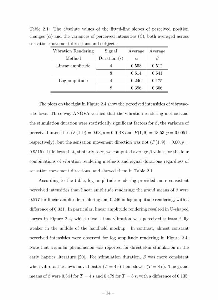
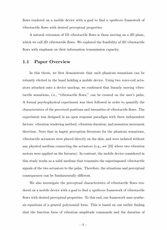
Table 2.1: The absolute values of the fitted-line slopes of perceived position

changes (α) and the variances of perceived intensities (β), both averaged across

sensation movement directions and subjects.

Vibration Rendering Signal Average Average

Method Duration (s) α β

Linear amplitude 4 0.558 0.512

8 0.614 0.641

Log amplitude 4 0.246 0.175

8 0.396 0.306

The plots on the right in Figure 2.4 show the perceived intensities of vibrotac-

tile flows. Three-way ANOVA verified that the vibration rendering method and

the stimulation duration were statistically significant factors for β, the variance of

perceived intensities (F (1, 9) = 9.03, p = 0.0148 and F (1, 9) = 13.53, p = 0.0051,

respectively), but the sensation movement direction was not (F (1, 9) = 0.00, p =

0.9515). It follows that, similarly to α, we computed average β values for the four

combinations of vibration rendering methods and signal durations regardless of

sensation movement directions, and showed them in Table 2.1.

According to the table, log amplitude rendering provided more consistent

perceived intensities than linear amplitude rendering; the grand means of β were

0.577 for linear amplitude rendering and 0.246 in log amplitude rendering, with a

difference of 0.331. In particular, linear amplitude rendering resulted in U-shaped

curves in Figure 2.4, which means that vibration was perceived substantially

weaker in the middle of the handheld mockup. In contrast, almost constant

perceived intensities were observed for log amplitude rendering in Figure 2.4.

Note that a similar phenomenon was reported for direct skin stimulation in the

early haptics literature [20]. For stimulation duration, β was more consistent

when vibrotactile flows moved faster (T = 4 s) than slower (T = 8 s). The grand

means of β were 0.344 for T = 4 s and 0.479 for T = 8 s, with a difference of 0.135.

– 14 –

Similarly to α, the vibration rendering method was a more important factor for

the consistency of perceived vibration intensities than the signal duration.

2.3 Discussion

The experimental results demonstrated that the sensation of vibrotactile flow

can be reliably created in a mobile device using only two vibrotactile actuators.

Among the three factors, different vibration rendering methods and signal du-

rations significantly altered the perceptual characteristics of vibrotactile flows,

but different stimulation movement directions did not. Linear amplitude render-

ing and slower sensation movements produced vibrotactile flows spanning in a

longer distance than log amplitude rendering and faster sensation movements,

respectively. This property can be useful in applications that require the high

discriminability of sensation movement directions, especially under environments

with other perceptual noises. In terms of the consistency of perceived intensity,

log amplitude rendering and faster sensation movements showed better perfor-

mance than linear amplitude rendering and slower sensation movements. Such

smoothly moving vibrotactile sensations can be advantageous in some applica-

tions, e.g., those communicating affection. The trade-off should be carefully

considered in designing a vibration rendering method and deciding associated

parameters, depending on the goals of applications.

After the experiment, we directly attached the two LRAs on the palm with-

out the device mockup. We could feel the phantom sensations, but they were

substantially weaker than what could be produced with the mockup. Interest-

ingly, it appears that the mockup greatly amplifies the sensations of vibrotactile

flow. An investigation for this issue, including the modeling of vibration propa-

gation dynamics in the mockup, is currently ongoing.

The vibrotactile flow adds a new dimension in designing vibrotactile effects

– 15 –

for a mobile device. First of all, it can increase the discriminability of tactons

by allowing spatiotemporal information coding [9]. Also, the spatial property of

vibrotactile flows is natural and intuitive, thus can greatly facilitate learning the

associated meanings of tactons. Although not tested in this paper, the vibro-

tactile flow is expected to improve an information transmission rate, as observed

in the early haptics literature for direct skin stimulation [20]. For actual appli-

cations, the vibrotactile flow can help produce realistic vibrotactile effects for

mobile games, e.g., for shooting an arrow. It can also be used together with some

GUI elements, such as a scroll bar, with an aim to enhance the inconvenience of

the current GUI in a mobile device.

– 16 –

III. Perceptual Analysis of 1D Vibrotactile

Flows

This chapter investigates the perceptual characteristics of vibrotactile flows

rendered on a mobile device with a goal to find a synthesis framework of vi-

brotactile flows with desired perceptual properties. We uses synthesis equations

of a general polynomial form extended from the amplitude inhibition algorithm

presented in the previous chapter (Chapter II). we carried out a perceptual exper-

iment to investigate the effects of the synthesis parameters on an expanded set of

perceptual variables, including sensation movement distance, sensation velocity

variation, sensation intensity variation, and the subjective confidence of flowlike

sensation.

3.1 Perceptual Analysis Framework

3.1.1 Device

We used a mockup made of acrylic resin (11×6×1 cm; 82 g) to represent

mobile devices. Two LRAs (LG Innotek; model MVMU-A360G; rated voltage

2.8 V (peak); nominal resonance frequency 175 Hz) were attached to the mockup,

one at each end (10 cm apart), as shown in Figure 3.1. An LRA is an industry-

standard variable reluctance actuator adopted in the vast majority of touchscreen

mobile devices. It relies on the resonance of mass and spring elements to produce

high-intensity vibrations with a fast response time. The two LRAs were powered

by a custom-made amplifier connected to a PC via a data acquisition card (NI;

PCI-6229) at a 10 kHz sampling rate.

To perceive vibrotactile flows from a mobile device, the most natural and

– 17 –

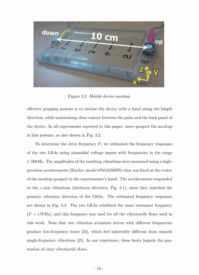
Figure 3.1: Mobile device mockup.

effective grasping posture is to enclose the device with a hand along the length

direction, while maintaining close contact between the palm and the back panel of

the device. In all experiments reported in this paper, users grasped the mockup

in this posture, as also shown in Fig. 3.2.

To determine the drive frequency F , we estimated the frequency responses

of the two LRAs using sinusoidal voltage inputs with frequencies in the range

1–500 Hz. The amplitudes of the resulting vibrations were measured using a high-

precision accelerometer (Kistler; model 8765A250M5) that was fixed at the center

of the mockup grasped in the experimenter’s hand. The accelerometer responded

to the z-axis vibrations (thickness direction; Fig. 3.1), since they matched the

primary vibration direction of the LRAs. The estimated frequency responses

are shown in Fig. 3.3. The two LRAs exhibited the same resonance frequency

(F = 178 Hz), and this frequency was used for all the vibrotactile flows used in

this work. Note that two vibration actuators driven with different frequencies

produce low-frequency beats [24], which feel inherently different from smooth

single-frequency vibrations [25]. In our experience, these beats impede the gen-

eration of clear vibrotactile flows.

– 18 –

Figure 3.2: Grasping posture of the mockup.

0 50 100 150 200 250 300 350 400 450 5000

0.2

0.4

0.6

0.8

Frequency (Hz)

Acce

lera

tion

(G)

Frequency: 178 HzMagnitude: 0.6819 G

Frequency: 178 HzMagnitude: 0.6650 G

Figure 3.3: Frequency responses of the two LRAs.

The next step was to calibrate the amplitude and phase characteristics of the

two LRAs. The vibration amplitudes driven with F = 178 Hz were measured for

each LRA using the accelerometer for 20 input amplitude levels. The measured

input-output relation was inverted for each LRA to determine the input voltage

amplitude required to produce a desired output acceleration amplitude. Further,

a non-zero phase offset existing between two sinusoidal waveforms reduces the

superimposed amplitude of the two waves. Thus, we found a phase offset be-

tween the LRAs by exhaustively searching the phase difference between the two

input waveforms that resulted in the largest output amplitude. This phase off-

set was 10 ◦, and it was used in rendering all the vibrotactile flows used in our

– 19 –

experiments.

3.1.2 Synthesis Functions

Research has found three effective approaches for vibrotactile flow rendering:

amplitude inhibition [14], time inhibition [13], and amplitude inhibition with a

frequency sweep [15]. The time inhibition method modulates the onset timings of

two vibrations and works well with ERMs [13]. In our experience, however, this

technique is ineffective for producing clear flow sensations with LRAs. With the

ERM that generally has correlated frequency-amplitude characteristics [26] and a

long rising time, varying the input signal duration (much shorter than the rising

time) also has the effect of changing the amplitude and frequency of the resulting

vibration. However, such complication does not occur with LRAs. Moreover,

the most recent approach in [15] enables the modulation of the spatial position

at which vibratory resonance occurs on a device plate by combining amplitude

inhibition with an input frequency sweep, but it requires the use of wideband

actuators, which are still very rare in commercial mobile devices. Therefore,

amplitude inhibition is the only viable option for LRAs.

The synthesis functions for vibrotactile flows we use are extended from the

amplitude inhibition algorithm for phantom sensations presented earlier by Al-

lies [20]. In our previous study [14], we tested two forms using linear and loga-

rithmic functions, and they were shown to produce vibrotactile flows of different

perceptual qualities on a mobile device. This result led us to consider the follow-

ing general input synthesis equations:

a1(t) = amax

(t

T

)γand a2(t) = amax

(1− t

T

)γ, (3.1)

where a1(t) and a2(t) are the respective acceleration amplitudes that the two

LRAs produce at time t, amax is the maximum acceleration (1.17 G in our hard-

ware setup), and T is the stimulus duration. With regards to t, these equations

– 20 –

00

a_max

Time

Acc

eler

atio

n

Vib 2

T

Vib 1

Figure 3.4: Vibrotactile flow synthesis functions.

are polynomials with a degree γ, which controls the shapes of the two functions,

as depicted in Figure 3.41. This synthesis rule was the best among the vari-

ous other function forms we tested in terms of simplicity and capability for flow

rendering.

To understand the relationship between the synthesis function and the vi-

bration output, we measured the acceleration of vibrotactile flows at different

positions on the device mockup. The measurement positions were on the center-

line in the height direction. A sample result is provided in Figure 3.5, which shows

that the vibration amplitude either decreased or increased over time, depending

on the position. These spatiotemporal distribution of vibrotactile stimuli induces

the phantom sensation that the vibration feels as if it is “flowing” from one end to

the other end. Moreover, changing the parameters in (4.1) can bring systematic

changes to the spatiotemporal distribution of vibrotactile stimuli, as illustrated

in Figure 3.5, and subsequently to the perceptual quality of the vibrotactile flows.

1This use of “tactile gamma” is adapted from gamma correction that is popular in video and

image systems [27].

– 21 –

Figure 3.5: Spatiotemporal distributions of the acceleration amplitudes when

vibrotactile flows were rendered through the mobile device mockup using the

synthesis function in (4.1) with T = 2 s. During the measurements, the device

mockup was grasped in the experimenter’s hand, and the accelerometer was at-

tached at the corresponding positions on the centerline on the front panel of the

mockup

. Each plot shows the averages of 0.4 s measurements. Note that the position is

a relative value.

3.2 Perceptual Characteristics

This section reports the perceptual experiment carried out to elucidate the

effects of the synthesis function parameters on the perception of vibrotactile flow.

– 22 –

3.2.1 Methods

Participants

Fifteen volunteers (19–27 years old with an average 21.0; 9 males and 6

females; all right-handed) participated in this experiment. All participants were

daily users of mobile phones with no known sensory impairments. They were

paid at a rate of KRW 10,000 (about USD 9) per hour after the experiment.

Experimental Conditions

To render vibrotactile flows, we varied the two independent variables, γ and

V . γ was selected from {0.25, 0.5, 1, 2, 4}, where the minimum and maximum

values had ensured the sensation of movement in pilot experiments. V is the

nominal velocity of sensation movement, and it also determines the duration T

of vibrotactile flow by V = 10 cm/T , where 10 cm is the distance between the

two LRAs. V was one of 3, 4, 7, 10, and 15 cm/s, which correspond to T of

3.33, 2.5, 1.43, 1, and 0.67 s, respectively. If V > 15 cm/s (T < 0.67 s), the flow-

like sensations are not salient, perhaps because of our perceptual limit, and the

occasions for V < 3 cm/s (T > 3.33 s) are rare in actual use. Combining the two

independent variables resulted in 25 different vibrotactile flows.

Procedures

An open response paradigm was used in the experiment. The participant’s

task in each trial was to perceive a vibrotactile flow generated though the mockup

grasped in their left hand and to draw two graphs to describe its perceptual

characteristics with his/her right hand using the GUI-based program shown in

Figure 3.6. The participants wore headphones that played white noise to block

out any auditory cue.

First, the participant was asked to draw a graph for the position of the

– 23 –

vibration sensation vs. (relative) time. The time was represented in a seven-point

scale from 0 to 6. The position was also shown in the same seven-point scale,

but each interval was further divided into three segments. Thus, the participant

could select a position from a total of 21 points between 0 and 6. This design was

revised from our previous study, which used only seven points for the position,

based on its questionnaire results [14]. Time levels 0 and 6 were defined as the

beginning and ending times of the vibrotactile stimulation, respectively, and the

position levels 0 and 6 as the positions of the LRAs at the bottom and top of

the mockup, respectively. The gradation of the position was also marked on the

device mockup. The participant was allowed to see the device mockup if it was

necessary to compare the perceived position of a vibrotactile flow and the marked

positions on the mockup. The participant could perceive the same vibrotactile

flow repeatedly by pressing the “Vibration” button on the GUI.

Second, the participant drew another graph for the perceived intensity against

time. The scales were the same as those of the position graph. A “Refer-

ence + Vibration” button on the GUI was used for this graph. Clicking this

button produced a reference stimulus by vibrating the LRA at the bottom of the

mockup for 1 s with an intensity of amax, followed by the vibrotactile flow. The

participant was instructed to regard intensity level 4 as the perceived intensity

of the reference stimulus and intensity level 0 as that of no vibration and then to

scale the perceived intensity of the vibrotactile flow accordingly, even in the case

that the vibrotactile flow felt stronger than the reference stimulus.

Lastly, the participants rated their subjective confidence about having felt a

“smooth and natural movement sensation” using a seven-point Likert scale (0–6).

The experiment began with a training session that consisted of 25 trials.

During each trial, each participant completed the above task for one of the 25

vibrotactile flows. The order in which the 25 vibrotactile flows were presented

– 24 –

Figure 3.6: GUI of the program used for the perceptual experiment.

was randomized for each participant. The main session was essentially the same

as the training session, except that each vibrotactile flow was repeated twice.

Only the results of these 50 trials were used for data analysis. The participants

had a 5-min break between the sessions. The experiment required about 1 h to

complete for each participant.

Perceptual Measures

To represent the perceptual quality of vibrotactile flows, we defined four

measures as follows: (1) Sensation movement distance D: The absolute difference

of the perceived positions between time 0 and 6. This variable quantifies the

perceived displacement of a vibrotactile flow. (2) Sensation velocity variation ∆v:

This measure gauges the perceived uniformity of vibrotactile flow movements. Let

pn (0 ≤ n ≤ 6) be the perceived position at time n. For each graph of pn and

n, a best-fitting line p = f(n) is found using linear regression. Then, ∆v =

maxn |pn − f(pn)|, indicating the maximum deviation of the perceived position

from the linear movements. (3) Sensation intensity variation ∆i: The difference

between the maximum and minimum of the perceived intensities, representing

– 25 –

0 1 2 3 4 5 60123456

0 1 2 3 4 5 60123456

0 1 2 3 4 5 60123456

0 1 2 3 4 5 60123456

0 1 2 3 4 5 60123456

0 1 2 3 4 5 60123456

0 1 2 3 4 5 60123456

0 1 2 3 4 5 60123456

0 1 2 3 4 5 60123456

0 1 2 3 4 5 60123456

0 1 2 3 4 5 60123456

0 1 2 3 4 5 60123456

0 1 2 3 4 5 60123456

0 1 2 3 4 5 60123456

0 1 2 3 4 5 60123456

0 1 2 3 4 5 60123456

0 1 2 3 4 5 60123456

0 1 2 3 4 5 60123456

0 1 2 3 4 5 60123456

0 1 2 3 4 5 60123456

0 1 2 3 4 5 60123456

0 1 2 3 4 5 60123456

0 1 2 3 4 5 60123456

0 1 2 3 4 5 60123456

0 1 2 3 4 5 60123456

V = 3(cm/s)

V = 15(cm/s)

V = 10(cm/s)

V = 7(cm/s)

V = 4(cm/s)

Figure 3.7: Plots of the perceived positions (filled circles) and the perceived

intensities (unfilled triangles) (y-axis) vs. time (x-axis). Note that all are relative

values.

the degree of perceived intensity changes. (4) Confidence rating CF : The rating

of subjective confidence about “smooth and natural sensation movements.” The

more a vibration felt like a flow, the higher the participants rated CF .

3.2.2 Results

We averaged the graphs for the perceived position and intensity across par-

ticipants for each experimental condition. The results are shown in Figure 3.7.

In all the plots, it is evident that the perceived position of the vibrotactile flows

changed monotonically.

The values of each of the four perceptual measures were computed from the

– 26 –

0

1

2

3

4

35

79

1113

15

2

3

4

5

6

7

V (cm/s)

D (c

m)

(a) Sensation movement distance D

01

23

4

03

57

911

1315

0.2

0.4

0.6

0.8

V (cm/s)

(b) Sensation velocity variation ∆v

01

23

4

0

35

79

1113

15

0.5

1

1.5

2

2.5

V (cm/s)

(c) Sensation intensity variation ∆i

01

23

4

03

57

911

1315

2.5

3

3.5

4

V (cm/s)

CF

(d) Confidence rating CF

Figure 3.8: Perceptual measures vs. γ and V . For each measure, measured data

and their best-fitting function are represented by circles and a meshed surface,

respectively.

data in Figure 3.7, and they are provided in Figure 3.8. The data distribution

of each measure passed the Shapiro-Wilk normality test with p < 0.0001. Thus,

we performed a two-way ANOVA for each measure to examine the statistical

significance of the two independent variables (γ and V ) and their interaction.

Then, mathematical functions that describe each perceptual measure with γ and

V were found using the best subset regression. Details are reported below for

each measure.

Sensation Movement Distance

The sensation movement distance D, shown in Figure 3.8(a), ranged from

2.13 to 6.96 cm. Considering that the distance between the two LRA was 10 cm,

– 27 –

this result indicates that the vibrotactile flows delivered clear movement sensa-

tions. Both γ and V had a statistically significant effect on D (F (4, 56) = 27.85,

p < 0.0001 and F (4, 56) = 11.58, p < 0.0001, respectively), but their interaction

did not (F(16, 224) = 0.80, p = 0.6802). The best-fitting regression model of D

(R2 = 0.94) was:

D = 1.25 ln γ − 0.133 V + 5.83. (3.2)

According to this equation, D increased logarithmically with γ, and it decreased

linearly with V . γ controls the spatial rate of vibration intensity changes, and

(3.2) suggests that γ is an effective indicator for the perception of sensation

movement distance. V is responsible for the temporal rate of vibration intensity

changes, but its effect on the sensation movement distance was weaker than that

of γ.

Sensation Velocity Variation

The data of sensation velocity variation ∆v are provided in Figure 3.8(b).

Its values were distributed between 0.18 and 0.75, and max ∆v/min ∆v = 4.23,

suggesting large differences of ∆v. Both γ and V were statistically significant for

∆v (F (4, 56) = 32.14, p < 0.0001 and F (4, 56) = 5.51, p = 0.0008, respectively),

but their interaction was not (F (16, 224) = 1.19, p = 0.2808). The best-fitting

model (R2 = 0.93) was:

∆v = 0.164 ln γ − 0.000795 V 3 + 0.0211 V 2 − 0.172 V + 0.892. (3.3)

Here, ∆v increased logarithmically with γ. Given γ, ∆v decreased, increased,

and then decreased again with V in a third-order polynomial form. This complex

behavior was due to the data points at V = 7 cm/s, which formed local minima

for all γ’s. However, whether the differences in ∆v around V = 7 cm/s are clearly

perceptible to users in actual applications is questionable.

– 28 –

Sensation Intensity Variation

The sensation intensity variation ∆i shown in Figure 3.8(c) varied between

0.12 and 2.53. As max ∆i/min ∆i = 20.81, the participants could reliably per-

ceive the changes in the intensity. Both γ and V were statistically significant for

∆i (F (4, 56) = 96.76, p < 0.0001 and F (4, 56) = 4.79, p = 0.0022, respectively),

as well as their interaction (F (16, 224) = 2.19, p = 0.0062). The best-fitting

function (R2 = 0.96) was:

∆i = 0.597 γ − 0.0154 γV + 0.253. (3.4)

This model indicates that ∆i increased linearly with γ, with a slope dependent

on V . ∆i decreased linearly with V , again with a slope dependent on γ.

Confidence Rating of Flow Sensation

The subjective ratings of the confidence of flow-like sensation, CF , are shown

in Figure 3.8(d). The ratings ranged from 2.47 to 3.97 (neutral: 3). Both γ and V

were statistically significant for CF (F (4, 56) = 3.55, p = 0.0119 and F (4, 56) =

6.28, p = 0.0003, respectively), but their interaction was not (F (16, 224) = 1.34,

p = 0.1756). The best-fitting regression model (R2 = 0.82) was:

CF = −0.290 γ2 + 1.27 γ − 0.354 lnV + 3.14. (3.5)

Hence, CF initially increased with γ, reached the highest confidence at γ ' 2,

and then began to decrease for γ > 2. CF was logarithmically decreased with V .

3.2.3 Discussion

The experimental results demonstrated that our synthesis function in (4.1)

can effectively control the perceptual characteristics of a vibrotactile flow. The

two synthesis parameters γ and V had statistically significant influence on all the

– 29 –

four perceptual metrics through well-defined functional relationships, which will

be called perceptual characteristic functions in the remainder of this paper.

The exact equations for the perceptual characteristic functions would depend

on the specific experimental setup. However, we expect that the general effects

of γ and V on the four perceptual measures would remain intact. We actually

tested different hardware setups by varying the distance between the two LRAs

(3–10 cm) and the weight of the device mockup (100, 120, and 140 g), even on a

thin plate (thickness < 0.2 cm). In all of these cases, the perceptual impression

of vibrotactile flows was consistent with the patterns predicted by the perceptual

characteristic functions. These results suggest that the perceptual characteristic

functions can be applied to different hardware setups after simple scaling.

3.3 Applications

The perceptual characteristic functions describe how our perception of a vi-

brotactile flow is affected by the parameters of the synthesis function. Therefore,

vibrotactile flows that have desired perceptual features can be designed using the

inverses of the perceptual characteristic functions. For example, in applications

that deliver the desired distance with directional information, the function for

D in (3.2) can provide a reference for selecting appropriate vibrotactile flows.

We actually implemented a bricks-breaking game (Arkanoid) in which the ball’s

movements and collisions are enhanced with vibrotactile flows. This game re-

ceived quite positive responses in informal user tests. Likewise, the perceptual

variable ∆v or ∆i can be essential for describing certain motions. In a golf game,

for instance, the movement of a golf ball in the vertical direction may be reflected

in the perceived velocity or intensity changes of a vibrotactile flow using (3.3) or

(3.4), respectively. If the precise delivery of the direction of vibrotactile flow is of

high priority, e.g., in navigation aids, the confidence rating CF in (3.5) deserves

– 30 –

more attention.

It should be remarked that the four perceptual measures are not independent

of each other; they are determined by two independent variables γ and V . For

example, our results suggest that it would be impossible to generate the vibro-

tactile flows that move in a short distance (low D) with high flow-like sensation

(high CF ). When D in Figure 3.8(a) is very low, the corresponding CF in Fig-

ure 3.8(d) is slightly less than 3 (the neutral score), indicating that the resulting

vibrations could feel like a flow, but not very clearly. On the other hand, if large

D is desired, ∆v and ∆i are also increased, while CF becomes low. This depen-

dency between the four perceptual characteristic functions needs to be carefully

taken into account for application design.

– 31 –

IV. Rendering of 2D Vibrotactile Flows:

Edge Flows

This chapter addresses the following three research ploblems as to edge flows:

• Information transmission capacity: The spatiotemporal nature of edge flows

was expected to improve the tactile information transmission capacity of

the current mobile platform. The first aim of this study was to quantify

the information transmission capacity of edge flows.

• Learning effect: We observed some need for learning, albeit short, for robust

identification of 1D vibrotactile flows [14, 28], as also mentioned in the

early studies on phantom sensations [20]. Our second goal was to assess the

learning effect of edge flows, which was expected to be higher than for 1D

flows.

• Need for correct-answer feedback: The last question pertains to the intu-

itiveness of edge flows; whether the learning requires correct-answer feed-

back. If practice without correct-answer feedback leads to performance

improvement comparable to practice with feedback, it indicates that edge

flows are sufficiently intuitive for users to learn by only trials and errors,

without the needs for additional learning procedures or user interfaces.

To find answers to the three research problems, we designed 32 edge flows

by changing their starting position, number of the 1D flows used, and rotation

direction. Then users ability to identify the 32 edge flows was evaluated in a

longitudinal user study (over a week). The experimental procedure on each day

was designed such that the practice was similar to what one would experience in

– 32 –

Vib 1 Vib 2

Vib 3Vib 4

Distal

Radial

Proximal

Ulnar

Figure 4.1: Mobile phone mockup and grasping posture used in the user study.

the daily use of a mobile device.

4.1 Methods

Our user study had three independent factors in a mixed-subjects design.

Within-subjects factors were edge flow and day of practice, while a between-

subjects factor was the use of correct-answer feedback. Details are presented

below.

4.1.1 Edge Flows

Edge flows consist of multiple, concatenated 1D vibrotactile flows. Our de-

sign of edge flows assumed the use of four vibrotactile actuators each of which is

placed at one of the four corners of a rectangular mobile device (Figure 4.1). The

geometric path of an edge flow can be uniquely defined by its starting edge (SE;

one of the four sides), the number of edges to span (NE; equal to the number of

1D flows to use), and rotation direction (RD; clockwise (CW) or counterclockwise

(CCW)). By limiting NE ≤ 4, we designed 32 (4 SE×4 NE×2 RD) paths of edge

flows, as shown in Figure 4.2.

Given an edge flow path, we also need to determine the algorithms to render

individual 1D flows and their parameters. We use our synthesis algorithm of 1D

– 33 –

Figure 4.2: Geometric paths of 32 edge flows.

vibrotactile flows introduced in the previous chapter (Chapter III). This algo-

rithm is based on amplitude inhibition and so suitable for LRAs. The synthesis

equations for a 1D flow that progresses from LRA 1 to LRA 2 are:

a1(t) = amax

(1− t

T

)γand a2(t) = amax

(t

T

)γ, (4.1)

where a1(t) and a2(t) are the respective accelerations that the two LRAs produce

at time t, amax is the maximum acceleration, and T is the stimulus duration.

With regard to t, the two functions are polynomials with a degree γ. For the

distance d between the two LRAs, T = d/v where v is the nominal velocity of

sensation movement.

Our previous study (Chapter III) showed that the two parameters, γ and

v (or T ), determine the perceptual characteristics of 1D vibrotactile flows, such

as movement distance of a sensation, variation in the velocity or the intensity

of a sensation, and the confidence of flow-like sensation. We could also find

mathematical functions that can be used to design vibrotactile flows with desired

perceptual properties. In order to render an edge flow, its constituent 1D flows are

generated successively by driving the corresponding actuators using the synthesis

equations in (4.1). An example is provided in Figure 4.3.

To render edge flows, we used a rectangular mobile phone mockup (11 cm×6 cm×1 cm)

– 34 –

0 0.5 1 1.5 2 2.5 3

x 104

0

0.2

0.4

0.6

0.8

1

Time (sec)

No

rmal

ized

Acc

eler

atio

n

Vib2 Vib3 Vib4 Vib1

Figure 4.3: Input acceleration profile of the edge flow at the bottom-left corner

of Figure 4.2. γ = 1. T = 0.5 s for short edges and 1 s for long edges.

made of acrylic resin. Participants grasped the mockup with their non-dominant

hand while enclosing the mockup with their palm and fingers (Figure 4.1). The

short ends of the mockup were indented by 0.5 cm. Four LRAs (LG Innotek

MVMU-A360G) were attached at the four corners on the indented region to

prevent direct contact of the LRAs to participants’ hand. The center-to-center

distance d between the LRAs was 10 cm along the long edges and 5 cm along the

short edges. The LRAs were controlled by a PC at a sampling rate of 10 kHz

using a data acquisition card (NI PCI-6723) and a power amplifier.

All the LRAs were driven at the same frequency (177 Hz). This frequency

allowed us to use the greatest common amplitude for the LRAs according to their

frequency responses. Note that using different frequencies create low-frequency

beats [29], and it hinders rendering clear flow-like sensations [14, 28]. We also

found the phase offset between each pair of the LRAs by exhaustively searching

for the phase difference that resulted in the largest output amplitude. This

was because a non-zero phase offset existing between two sinusoidal waveforms

– 35 –

reduces the superimposed amplitude of the two waves. Lastly, to produce desired

acceleration amplitudes, the required input voltage amplitudes were obtained

from a measured input-output relationship for each LRA. Further details of these

calibration procedures are described in [28].

Other specific synthesis parameters were as follows: (1) amax = 0.36 G—

the maximum amplitude that the four LRAs could commonly produce at 177 Hz

when the mockup was grasped in the hand, corresponding to about 35.44 dB SL

using the absolute threshold taken from [26]; (2) v = 10 cm/s—therefore T = 1 s

on the long edges (d = 10 cm) and 0.5 s on the short edges (d = 5 cm). The total

durations of the edge flows varied between 0.5 and 3 s; (3) γ = 1—to provide

vibrotactile flows with uniform perceived intensities and velocities over time [28].

4.1.2 Procedure

The experiment for each participant consisted of five practice sessions con-

ducted on five consecutive days and one delayed recall test performed two or

three days (depending on the participant’s availability) after the practice.

Each practice session proceeded as follows. First, the participant was pre-

sented with the 32 edge flows, twice each, in the order shown in Figure 4.2 (left

to right, then top to bottom). During the playback of each edge flow, a graphical

user interface (GUI), which looked similar to Figure 4.2, highlighted the visual

icon that represented the movement of the edge flow. The next edge flow started

2 s later to prevent tactile adaptation. Second, the participant went through 128

practice trials (32 edge flows×4 repetitions). On each trial, the participant per-

ceived a randomly-selected edge flow, and then answered which edge flow was

perceived by clicking the corresponding icon on the GUI program using a mouse.

The participant could perceive the edge flow as many times as s/he needed. After

the response, the correct answer was highlighted on the GUI program for visual

– 36 –

feedback. This feedback was optional depending on the condition to which the

participant was assigned. Lastly, an immediate recall test followed, wherein the

32 edge flows were presented only once in a random order. The procedure was the

same as that of the practice, except that no correct-answer feedback was given.

One-day practice sessions were finished in approximately one hour.

The delayed recall test had the same procedure as the immediate recall

tests in the practice sessions. It is noted that all the recall tests did not have

repetitions, testing each edge flow only once. This was to make the recall tests

as brief as possible; including repetitions in recall tests also provides practice to

some extent.

Throughout the experiment, the participants wore noise-cancelling head-

phones to block the faint sound generated by the LRAs. The participants were

allowed to take a break whenever necessary.

4.1.3 Participants

We recruited 20 participants for this experiment. Ten of them (five male

and five female; 19–26 years old with a mean 20.7) were tested with no correct-

answer feedback, while the other ten (five male and five female; 19–26 years old

with a mean 21.8) were with correct-answer feedback. All of the participants

were right-handed and daily users of a mobile phone. None of them reported

known sensory impairment. The participants signed on a standard consent form

prior to the experiment. They were paid KRW 10,000 (about USD 10) per hour

after the experiment.

4.1.4 Performance Measures

We used the experimental data collected in the five immediate recall tests and

the one delayed recall test for data analysis. For each recall test, the data of the

ten participants measured under the same correct-answer feedback condition were

– 37 –

pooled to compute a stimulus-response confusion matrix. This confusion matrix

was used to obtain the maximum likelihood estimate of information transfer IT

using the standard formula [30]. This procedure results in only one IT for each

recall test and correct-answer feedback condition.

IT represents how many bits of information the participants could identify

from the 32 edge flows. IT is a unit-free measure of human performance that

allows for comparisons across different modalities and displays [30]. 2IT corre-

sponds to the maximum number of edge flows that could be recognized without

errors.

Another performance metric we used is the percent correct PC of each edge

flow. Examination of PC enables us to find edge flows with high identifiability,

and such knowledge is indispensable for the development of actual applications.

However, PC is not appropriate for comparisons between different cases unlike

IT. Even for the same stimuli, PC generally decreases with a larger stimulus set,

but it does not necessarily imply that the total number of identifiable stimuli

have decreased [31].

4.2 Results

4.2.1 Information Transfer

Figure 4.4 shows the values of IT measured in the five immediate recall tests

after the practice of each day and the delayed recall test. Note that the maximum

achievable IT was 5 bits (32 edge flows).

Without correct-answer feedback, IT increased with practice, and it was the

greatest at the delayed recall test with IT = 3.39 bits and 2IT = 10.5. This

improvement corresponds to 15% in IT and 36% in 2IT compared to the lowest

performance measured on day 1 (IT = 2.95 bits and 2IT = 7.7). With correct-

answer feedback, IT also increased with practice in general, but the greatest value

– 38 –

Figure 4.4: IT estimates measured in the immediate and delayed recall tests.

was measured on day 5 with IT = 3.72 bits and 2IT = 13.2. The performance

at the delayed recall test was slightly lower with IT = 3.70 bits and 2IT = 13.0.

This is an improvement of 17% in IT and 44% in 2IT compared to the lowest

performance of day 1 (IT = 3.17 bits and 2IT = 9.0).

All IT values obtained with correct-answer feedback were higher than the

corresponding ITs without correct-answer feedback. A two-sample t-test showed

that the mean difference of IT between the two feedback conditions was statisti-

cally significant (p = 0.0092). Statistical tests for learning effect was not possible

because only one IT value was available for each experiment day.

– 39 –

Figure 4.5: Percent correct scores. Error bars represent standard errors. Letters

A and B indicate the results of a Tukey’s HSD test for experiment day (A: a

higher performance group and B: a lower performance group).

4.2.2 Percent Correct

Figure 4.5 shows the mean PC values averaged across edge flows and par-

ticipants. The graphs exhibit similar trends to the graphs of IT in Figure 4.4.

Without correct-answer feedback, the mean PC improved from 44.4% on day

1 to 57.8% at the delayed recall test. With correct-answer feedback, the mean

PC increased from 52.5% on day 1 to 67.2% at the delayed recall test, with a

maximum of 70% on day 5.

For each edge flow, the PC values of the ten participants who had a practice

under the same correct-answer feedback condition were averaged for each ex-

periment day. Then, we conducted a two-way mixed-design ANOVA on PC with

– 40 –

experiment day as a within-subjects factor and correct-answer feedback condition

as a between-subjects factor. The effect of experiment day was statistically signif-

icant (F (5, 90) = 3.03, p = 0.0143). The effect of correct-answer feedback was not

significant but close to the significance level (F (1, 18) = 3.13, p = 0.0938). We

then performed a Tukey’s HSD test for multiple comparisons to further investigate

the effects of experiment day. The results are marked in Figure 4.5 using symbols,

which indicate learning effects more clearly than the data of IT. The interaction

term between the two factors was not significant (F (5, 90) = 0.44, p = 0.8208).

4.3 Discussion

4.3.1 Information Transmission Capacity

Our design of the 32 edge flows resulted in the highest IT of 3.70 bits at

the delayed recall test after the participants had practiced for five days with

correct-answer feedback. This value of IT means, at least theoretically, that we

can recognize 13 edge flows with no errors.

The IT of our edge flows outperforms those reported in the following previous

studies that used a single vibrotactile actuator: 1.76 bits—8 tactons that varied

in amplitude, frequency, and pulse duration [7]; 2.5 bits—12 key-click signals

with different amplitudes, frequencies, and the number of pulses [31]. The IT

of our study is also higher than those reported earlier using multiple actuators:

1.99 bits—18 tactor locations of two 3×3 tactor arrays placed on the dorsal and

volar sides of the wrist [32]; 1.90–2.49 bits—8 tactile patterns using 4 voice coil

actuators around the wrist [33]; 2.46 bits—9 locations with a 3×3 motor array

affixed to the palm [34]; 3.37 bits—27 tactons with different rhythms, roughnesses,

and spatial locations using 3 voice coil actuators stimulating the forearm [35].

However, the IT of our edge flows was smaller than those reported in [12, 36]:

4.28 bits—24 vibration patterns generated using 3 vibration motors in a wrist-

– 41 –

band tactile display by changing their intensity, temporal pattern, starting point,

and direction; 6.5 bits–120 stimuli using 4 finger configurations (thumb, index

finger, middle finger, or all of them) and 30 waveforms with different frequencies

and amplitudes. Note that accurate localization was enabled with those tactile

stimuli.

The above comparisons indicate that the IT of edge flows is among the best

that has been reported in the literature, even though edge flows do not require

precise localization. We expect that the IT of edge flows can be further improved

if other temporal factors, such as intensity, duration, and γ, are also considered

in the design, similarly to [12].

4.3.2 Learning Effect

The performance improvement obtained by five-day practice was 15% in IT

and 36% in 2IT without correct-answer feedback, and it was 17% in IT and 44%

in 2IT with correct-answer feedback (Section 4.2.1). This can be regarded as a

considerable learning effect, although formal statistical tests were not allowed for

IT (only one value per condition). The learning effect manifested itself in the

results of percent correct PC, for which the effect of practice was statistically

significant (Section 4.2.2). In addition, examining Figure 4.4 and 4.5 suggests

that the learning took place quickly; it could have reached a plateau as early as

on day 3. Note that IT and PC on day 4 showed a decreasing tendency, but we

are not certain of reasons at the moment.

Therefore, we can conclude that robust recognition of edge flows requires

some practice, presumably due to their illusory nature. The learning can be

done relatively quickly, however, possibly owing to their intuitive spatiotemporal

characteristics.

– 42 –

4.3.3 Need for Correct-Answer Feedback

In terms of IT, providing correct-answer feedback during learning was help-

ful, leading to a statistically significant difference compared to the control con-

dition of no correct-answer feedback (Section 4.2.1). As for PC, it was improved

by correct-answer feedback, but not to the level of statistical significance, albeit

the p-value (≈ 0.09) that approached significance (Section 4.2.2). At the delayed

recall test, the extent of improvement enabled by correct-answer feedback was

9% in IT, 24% in 2IT, and 16% in PC.

These results validate that correct-answer feedback is instrumental in im-

proving the users’ percent correct of edge flows. It is nonetheless worth mention-

ing that the performance improvement achieved by repeated practice was greater

than that by correct-answer feedback.

4.3.4 Edge Flows with High Percent Correct Scores

In actual uses of edge flows, designers need to select the edge flows with the

highest percept correct scores such that the number of selected edge flows is close

to 2IT = 13. We selected such a set of edge flows using the method presented

in [31]. We first sorted the 32 edge flows in a descending order of the mean

PC measured in the delayed recall test. Beginning from the edge flow with the

highest mean PC, we added each edge flow to the set one by one if the edge flow

had low confusion rates with other edge flows already included in the set. The

13 best edge flows obtained in this way are shown in Figure 4.6. Stimuli chosen

in this way retain the IT of the original stimulus set with almost perfect percent

correct scores [31].

Then, we moved our attention to the means PCs for the three design variables

measured in the delayed recall test (averaged between the two correct-answer

feedback conditions), which are shown in Figure 4.7. The edge flows that start

– 43 –

0.85 0.50 0.70 0.85 0.50 0.55 0.65 0.65

0.65 0.60 0.60 0.60 0.60 0.55 0.60 0.70

0.60 0.55 0.50 0.60 0.60 0.60 0.80 0.70

0.60 0.55 0.60 0.60 0.75 0.80 0.45 0.55

Exp I Exp II

Avr

내보내기 -> pdf 게시로 하면 그림 더 깔끔한듯

Ret days

1 26

45

73

9 10

11 13 8

12

Figure 4.6: Mean PCs of individual edge flows measured in the delayed recall

test. A number within each symbol represents the mean PC of the corresponding

edge flow. The best 13 edge flows for uses in applications are highlighted and

also ranked.

Figure 4.7: Means PCs measured in the delayed recall test for the three design

variables of edge flows. Error bars represent standard errors.

at the ulnar side of the hand resulted in a substantially higher PC than the other

edge flows (Figure 4.7(a)). The other three starting edges showed similar PCs.

We are not aware of particular grounds for this behavior at the moment. As

for the number of edges, NE = 1 showed the highest mean PC (Figure 4.7(b)),

indicating that the simplest edge flows can be easier for identification than the

other concatenated flows. The other edge flows with 2 ≤ NE ≤ 4 resulted in

similar PCs. Lastly, we were not able to find a noticeable difference in the mean

PC between the two rotating directions of edge flows (Figure 4.7(c)). Note that

we did not carry out further statistical analyses because of an insufficient number

of data samples. Probing the effects of the three design variables of edge flows

– 44 –

can be an interesting topic for future research.

– 45 –

V. Conclusion

In this thesis, we presented the design and results of a perceptual experi-

ment that measured the performance of creating a linearly moving vibrotactile

sensation on the user’s palm holding a mobile device using only two vibrotac-

tile actuators. The important contributions of this work can be summarized as:

1) Demonstration of the feasibility of the use of spatial vibrotactile stimulation

for interaction with a mobile device and 2) Providing the trade-off in designing

vibrotactile flows appropriate for the goals of applications.

In addition, ability of vibrotactile flows to produce diverse perceptual effects

were studied. To this end, we used a polynomial-form synthesis function with

two independent parameters of tactile gamma (the degree of the polynomial) and

duration (or nominal movement velocity). The results of our perceptual experi-

ment showed that these parameters can control the perceptual characteristics of

vibrotactile flows in systematic manner.

Moreover, we have proposed to study edge flows as a first step to extend

1D vibrotactile flows to 2D. Edge flows consist of multiple, concatenated 1D

vibrotactile flows rendered along the four edges of a rectangular mobile device

using four actuators. We carried out a longitudinal user study over one week with

20 participants in order to investigate the information transmission capacity of

edge flows, as well as the effects of practice and correct-answer feedback. The

IT of edge flows was as high as 3.70 bits, being greater than the IT reported

in the majority of previous studies pertaining to information transmission via

the tactile sense. We found both repeated practice and correct-answer feedback

beneficial for the improvement of edge flow identification. The learning could be

done quickly in a few sessions, and repeated practice enabled higher performance

– 46 –

enhancement than correct-answer feedback. The contributions of this study can

be summarized to: (1) the first proposal of edge flows as a means to improve the

information transmission capacity of mobile devices and (2) a quantification of

the benefits of repeated practice and correct-answer feedback for users’ accurate

recognition of edge flows.

– 47 –

요 약 문

진동 흐름이란 모바일 기기 표면 상에 연속적으로 움직이는 듯한 느낌 혹은 구현

방법을 일컫는다. 먼저 두 개의 진동자를 모바일 기기 상에 배치하였을 때 진동

흐름의 구현 가능성을 사용자 평가 실험을 통해 알아보았다. 이 실험에서 사용자는

인지되는진동의위치와세기를시간에따라그래프로그렸다. 그결과,이러한진동

흐름이 충분히 구현 가능한 것임을 확인할 수 있었으며, 더욱 부드럽고 명확한 진동

흐름을 위해서는 렌더링 방법과 지속 시간 간의 조율이 필요하다는 것을 알아내었

다. 이를 바탕으로 진동 흐름의 인지적 특성을 파악하는 연구를 수행하였고, 원하는

인지적 특성을 갖춘 진동 흐름을 구현할 수 있는 제작 방법을 제안하였다. 이러한 1

차원상의진동흐름연구에서나아가서, edge flow라는네개의진동자를직사각형

의코너에배치하여이를따라돌아가는 2차원상의진동흐름의연구로확장하였다.

32개의 edge flow를디자인하고정보전달량과학습에필요한조건을알아보기위한

수일에 걸친 사용자 실험을 수행하였다. 그 결과 edge flow는 3.70 비트의 정보를

전달하는 것을 확인하였으며, 단기간의 연습으로 쉽게 학습이 되었다.

– 48 –

References

[1] Jane Hwang, Jaehoon Jung, Sunghoon Yim, Jaeyoung Cheon, Sungkil Lee,

Seungmoon Choi, and Gerard J. Kim. Requirements, implementation, and

applications of hand-held virtual reality. International Journal of Virtual

Reality, 5(2):59–66, 2006.

[2] Eve Hoggan, Stephen A. Brewster, and Jody Johnston. Investigating the

effectiveness of tactile feedback for mobile touchscreens. In Proceeding of

the SIGCHI Conference on Human Factors in Computing Systems, pages

1573–1582. ACM, 2008.

[3] D. Wagner and D. Schmalstieg. First steps towards handheld augmented

reality. In Proceedings of the IEEE International Symposium on Wearable

Computers, pages 127–135, 2003.

[4] Eric Gunther. Skinscape: A tool for composition in the tactile modality.

Master’s thesis, Massachusetts Institute of Technology, 2001.

[5] Ronald T. Verrillo and George A. Gescheider. Perception via the sense of

touch. In Ian R. Summers, editor, Tactile Aids for the Hearing Impaired,

pages 1–36. Whurr Publishers Ltd, 19B Compton Terrace, London N1 2UN,

England, 1992.

[6] Jonghyun Ryu, Chil-Woo Lee, and Seungmoon Choi. Improving vibrotactile

pattern identification for mobile devices using perceptually transparent ren-

dering. In Proceedings of the International Conference on Human-Computer

Interaction with Mobile Devices and Services (MobileHCI), pages 257–260.

ACM, 2010.

– 49 –

[7] M. Azadi and L. Jones. Identification of vibrotactile patterns: Building

blocks for tactons. In Proceedings of the IEEE World Haptics Conference

(WHC), pages 347–352, 2013.

[8] Karen E. MacLean. Foundations of transparency in tactile information de-

sign. IEEE Transactions on Haptics, 1(2):84–95, 2008.

[9] Eve Hoggan, Sohail Anwar, and Stephen A. Brewster. Mobile multi-actuator

tactile displays. In Lecture Notes on Computer Science (HAID 2007), volume

LNCS 4813, pages 22–33, 2007.

[10] Alireza Sahami, Paul Holleis, Albrecht Schmidt, and Jonna Hakkila. Rich

tactile output on mobile devices. In Proceedings of the European Conference

on Ambient Intelligence, pages 210–221, 2008.

[11] Seungmoon Choi and Katherine J. Kuchenbecker. Vibrotactile display: Per-

ception, technology, and applications. Proceedings of the IEEE, 101(9):2093–

2104, 2013.

[12] Seungyon ”Claire” Lee and Thad Starner. Buzzwear: Alert perception in

wearable tactile displays on the wrist. In Proceedings of the ACM SIGCHI

Conference on Human Factors in Computing Systems (CHI), pages 433–442,

2010.

[13] S.Y. Kim, J.O. Kim, and K. Kim. Traveling vibrotactile wave–A new vi-

brotactile rendering method for mobile devices. IEEE Transactions on Con-

sumer Electronics, 55(3):1032–1038, 2009.

[14] J. Seo and S. Choi. Initial study for creating linearly moving vibrotactile

sensation on mobile device. In Proceedings of the Haptics Symposium, pages

67–70. IEEE, 2010.

– 50 –

[15] J. Kang, J. Lee, H. Kim, K. Cho, S. Wang, and J. Ryu. Smooth vibrotactile

flow generation using two piezoelectric actuators. IEEE Transactions on

Haptics, 5(1):21–32, 2012.

[16] Sang-Youn Kim and Jeong Cheol Kim. Vibrotactile rendering for a travel-

ing vibrotactile wave based on a haptic processor. IEEE Transactions on

Haptics, 5(1):14–20, 2012.

[17] K. Yatani and K. N. Truong. SemFeel: A user interface with semantic

tactile feedback for mobile touch-screen devices. In Proceedings of the ACM

Symposium on User Interface Software and Technology, pages 111–120, 2009.

[18] Linda R. Elliott, Jan B.F. van Erp, Elizabeth S. Redden, and Maaike Duis-

termaat. Field-based validation of a tactile navigation device. IEEE Trans-

actions on Haptics, 3(2):78–87, 2010.

[19] C. E. Sherrick and R. Rogers. Apparent haptic movement. Perception &

Psychophysics, 1:175–180, 1966.

[20] David S. Allies. Information transmission by phantom sensations. IEEE

Transactions on Man-Machine Systems, 11(1):85–91, 1970.

[21] S. Tachi, K. Tanie, K. Komiyama, K. Asaba, Y. Tomita, and M. Abe. Infor-

mation transmission by two-dimensional electrocutaneous phantom sensa-

tion. In Proceedings of the 8th Annual Northeast Bioengineering Conference,

pages 258–262, 1980.

[22] Ali Israr and Ivan Poupyrev. Tactile brush: Drawing on skin with a tactile

grid display. In Proceedings of the ACM SIGCHI Annual Conference on

Human Factors in Computing Systems, pages 2019–2028, 2011.

[23] Jongeun Cha, Lara Rahal, and A. E. Saddick. A pilot study on simulating

continuous sensation with two vibrating motors. In Proceedings of the IEEE

– 51 –

International Workshop on Haptic Audio Visual Environments and their

Applications, pages 143–147, 2008.

[24] Y. Yoo, I. Hwang, and S. Choi. Consonance perception of vibrotactile chords:

A feasibility study. In Lecture Notes on Computer Science (HAID 2011),

volume LNCS 6851, pages 42–51, 2011.

[25] G. Park and S. Choi. Perceptual space of amplitude-modulated vibrotactile

stimuli. In Proceedings of the IEEE World Haptics Conference, pages 59–64,

2011.

[26] J. Ryu, J. Jung, G. Park, and S. Choi. Psychophysical model for vibrotactile

rendering in mobile devices. Presence: Teleoperators and Virtual Environ-

ments, 19(4):364–387, 2010.

[27] C. A. Poynton. Digital video and HDTV: algorithms and interfaces. Morgan

Kaufmann, 2003.

[28] J. Seo and S. Choi. Perceptual analysis of vibrotactile flows on a mobile

device. IEEE Transactions on Haptics, 6(4):522–527, 2013.

[29] Y. Yoo, I. Hwang, and S. Choi. Consonance of vibrotactile chords. IEEE

Transactions on Haptics, 7(1):3–13, 2014.

[30] Hong Z. Tan, Charlotte M. Reed, and Nathaniel I. Durlach. Optimum infor-

mation transfer rates for communication through haptic and other sensory

modalities. IEEE Transactions on Haptics, 3:98–108, 2010.

[31] Hsiang-Yu Chen, Jaeyoung Park, Steve Dai, and Hong Z. Tan. Design and

evaluation of identifiable key-click signals for mobile devices. IEEE Trans-

actions on Haptics, 4(4):229–241, 2011.

– 52 –

[32] H. Chen, J. Santos, M. Graves, K. Kim, and H. Z. Tan. Tactor localization

at the wrist. In Lecture Notes in Computer Science, volume 5024, pages

209–218, 2008.

[33] M. Matscheko, Johannes Kepler, Linz Linz, A. Ferscha, A. Riener, and

M. Lehner. Tactor placement in wrist worn wearables. In Proceedings of

IEEE International Sympsoium on Wearable Computing (ISWC), pages 1–

8, 2010.

[34] Katherine O. Sofia and Lynette A. Jones. Mechanical and psychophysical

studies of surface wave propagation during vibrotactile stimulation. IEEE

Transactions on Haptics, 6:320–329, 2013.

[35] Lorna M. Brown and Topi Kaaresoja. Feel who’s talking: Using tactons for

mobile phone alerts. In CHI ’06 Extended Abstracts on Human Factors in

Computing Systems, pages 604–609, 2006.

[36] Hong Z Tan, Nathaniel I Durlach, Charlotte M Reed, and William M Ra-

binowitz. Information transmission with a multifinger tactual display. Per-

ception & Psychophysics, 61(6):993–1008, 1999.

– 53 –

Acknowledgements

지도교수님이신최승문교수님께먼저감사의말씀을드립니다. 부족한점이많은

저였지만 끝까지 넓은 아량으로 지도해 주신 덕에 너무나도 많은 것을 배울 수 있

었던 과정이었습니다. 일에 대한 열정과 추진력, 빠르고 정확한 판단력과 전달력은

평생 본받을 점으로 간직할 것입니다. 긴 과정동안 아낌없는 조언과 도움을 주신

부분이 너무 많아 감사의 표현만으로는 부족하지만, 앞으로 잊지 않고 최선을 다해

나아가는 것으로 보답해드리려 합니다.

논문심사에 와서 아낌없는 조언을 주신 한성호 교수님과 안희갑 교수님, 그리고

이승용 교수님과 정홍 교수님, 조민수 교수님께도 감사의 말씀을 드립니다. 바쁜

와중에도 참석해주셔서 제가 연구한 부분에서 부족한 점이 무엇인지 깨닫고 더욱

발전된 방향으로 다질 수 있도록 큰 도움을 주셔서 감사드립니다.

Haptics and Virtual Reality 연구실의 선후배들에게도 고마음을 표현합니다. 성

길이형, 석희형, 종현이형, 성훈이형, 재봉이형, Reza, Amit, 인욱이형, 갑종이형,

인이형, 건혁이형, 경표형, 명찬이형, Phoung, 준석이, 호진이, 성환이, 용재, 호준

이, 종호, 승재, 한슬이, 인석이, 성호, 상윤이, 선웅이, 겨례, 성원이, 혜진이, 채용이,

효승이 등 너무나도 많은 선후배들에게 많은 배움과 도움을 받았습니다. 또한 행

정직을 담당하신 송이 선생님과 EDEN 연구실의 재민이형과 승환이에게도 그간의

과정에 도움을 받았습니다. 이들에게 준 것보다 받은 것이 너무 많아 감사할 따름이

고, 한 편으로는 제가 더 많이 주지 못해 아쉽고 미안합니다.

마지막으로 이 과정을 묵묵히 지켜주고 도와준 가족들, 그리고 사랑스런 아내

보영이와 자랑스런 아들 범수에게 앞으로 더욱 더 발전된 모습을 보여줄 것을 약

속하며 희망찬 발걸음을 앞두고 그 간의 모든 분들꼐 사랑과 고마움을 전하며 글을

마칩니다.

Curriculum Vitae

Name : Jongman Seo

Education

2005. 3. – 2009. 2. Department of Computer Science and Engineering, Pohang

University of Science and Technology (POSTECH) (B.S.)

2009. 3. – 2018. 8. Department of Computer Science and Engineering, Pohang

University of Science and Technology (POSTECH) (M.S.)