1  

Perceiving traffic environmental information based on driving scene

computational model

Yuren Chen, Ruoyu Liao, Yongxin Ye, Zuxing Liao

Traffic Engineering School of Tongji University 4800 Cao an Highway, Shanghai, China, 201804

Tel. 0086(21)69585717 Email chenyr@tongji.edu.cn

Submitted to the 3rd International Conference on Road Safety and Simulation,   September 14‐16, 2011, Indianapolis, USA 

Abstract: A driver achieves perception information from traffic environment  by vision scenes instead of knowing concrete road design parameters during his driving activity. Traffic environmental information is mainly shown to drivers as driving vision scenes. Driving vision scenes are a series of two dimensional visual images shaped from three dimensional objects (e.g. highway, vehicles, roadside and surroundings along the highway). They are the most important perception sources for drivers to gain information and satisfy driving demands. During driving process, a driver combines observed environment information with his general knowledge together to derive actions which are divided into accelerating,  decelerating and keeping constant velocity. This paper focused on perceiving lanes and vehicles information based on driving scene, then relationship is studied between these information and velocity change. A driving scene computational model is established based on “foreground” and “background”. What can be defined as the “background” includes the sky, road pavement and roadside environment. Correspondingly, the rest is defined as “foreground”, which is constituted of vehicles as well as pedestrians. Then, operating speed and driving scene are collected through naturalistic driving survey equipment. A further analysis on the potentially of driving scene in fields such as traffic security assessment, traffic risk profile and driving acceleration and deceleration are discussed. Key words: driving vision scene; computational model; background and foreground; acceleration and deceleration; 1. INTRODUCTION

Vehicle driving is a complex activity which requires that drivers (i) achieve

perception information from traffic environment, (ii) understand driving situation from other drivers, (iii) and make decision to interact vehicles with dynamic environment. All these tasks could be classified into environment representation, visual perception and decision making involve driver cognition with driving scenes.

2  

Sometime, such information is not sufficient for drivers to make a correct decision and misleading information make it easy for drivers to make mistakes. This is the reason why collision statistics show that over 90% of highway collisions are caused by driver error. Obviously, driving scene plays as a very import role in driving activities. In fact, the driving scene is a series of 2D vision images which are shaped from 3D objects (e.g. highway, vehicles, roadside and surroundings along highway) in driver’s eyes. Driving scenes are the most important perception sources for a driver to gain information and meet visual demand. It not only offers a visual environment for calm but also improves traffic safety (FHWA, 1999). Generally speaking, driving would involve traffic accident risk and driving scenes can be applied to prevent traffic accidents and to warn drivers traffic accidents advanced. They are mainly used in driving assistance, such as to detect and track vehicles (Chen, 2009), as dynamic visual model to reduce traffic risk (Cherng, 2009), to keep lane estimation and tracking vehicles (Mccall, 2006). Armingol created IVVI system which aimed at automatic driving and focused on the comprehension of driving scene (Armingol, 2007). It only simply utilized image recognition process without think of the random movement of vehicles on road. Messelodi employed visual information to detect and recognize vehicles at intersections (Messelodi, 2005). Leibe made detection based on the moving vehicles as real time targets using method of image technology (Leibe, 2008). Liu employed binocular stereovision method (Liu, 2004) while Malinovskiy used monocular stereovision (Malinovskiy, 2008). Gandhi used fixed background (Gandhi, 2007) and Gavrila employed mobile background method (Gavrila, 2007). Sotelo attempted to detect lanes on roads with no markings (Sotelo, 2004). Hsu made a macro introduction on the method of real time wheel path trace on road (Hsu, 2005) and Wang studied keeping lane by positioning technology (Wang, 2004). Wang employed B-line in lane detection and keeping, he got fine research achievement (Wang, 2005). Dewaard studied the effect of layout and environment design on behaviors and psychological aspects of drivers (Dewaard, 1995). AI-Shihabi came up with a more effective driver’s behavior model for driving simulation (AI-Shihabi, 2003). At the same time Easa researched a typical sight image model featuring driving scene on 3-D alignment (Easa, 2006). Kumar studied framework of driver’s real time behavior based on sequence image (Kumar, 2005). Kastrinaki gave a comprehensive view on the use of continuous image technology in traffic engineering (Kastrinaki, 2003) while Enkelmann did research on the use of driving vision technology in establishment of driving assistant (Enkelmann, 2001), etc.

These existing researches have confirmed that changes in road geometric alignment would impact driver vision scene, and different perception views would affect driver operating speed. Drivers operate vehicles mainly based on perspective view instead of reading geometric parameter directly. In two dimensional image, some traffic parameters such as road design parameters, road lanes and frontal vehicle that in current lane can be extracted and quantified to reach at target of driving safety. In this paper, the rear-end crash risk is picked up as a typical example to introduce our idea. Image processing can help us judge and identify vehicles velocity change between host vehicles to target vehicle ahead in same lanes. Section 2, circularity and

3  

orientation are used to judge and calibrate parameters of lanes; Section 3 will introduce a method using calibrated lane to perceive relative speed between target vehicle and host vehicle. Section 4 will put forward an application which could assist us to know potential rear-end risks early in highway. 2, METHODOLOGY 2.1 Hierarchy Structure of Driving Scene

The process of driving was described as a control loop system. More than about 90% of information required for driving task is perceived from driver visual. Drivers perceive environment mainly through sensors such as eyes and ears to gain information. The processor (driver brain) uses gained information together with general knowledge about driving and characteristics about road to derive the actions. The actions which driver performs affect vehicle controls and traffic safety. The challenge is that we should understand which parts of visual information play important roles during driving process and we should know how to model perception of visual information. Drivers may maintain a relatively high or low speed when the highway curves are perceived flat or sharp. The erroneous driver perception has been particularly evident when horizontal and vertical curves overlap irrelevantly. The combination of a sag vertical curve with a horizontal curve may result in a perspective view that makes horizontal curve appear flatter than it is in reality, whereas the combination with a crest vertical curve reveals opposite results. It may be hazardous if the drivers perceive a sharp curve as a flat curve, and subsequently adopts a higher speed.

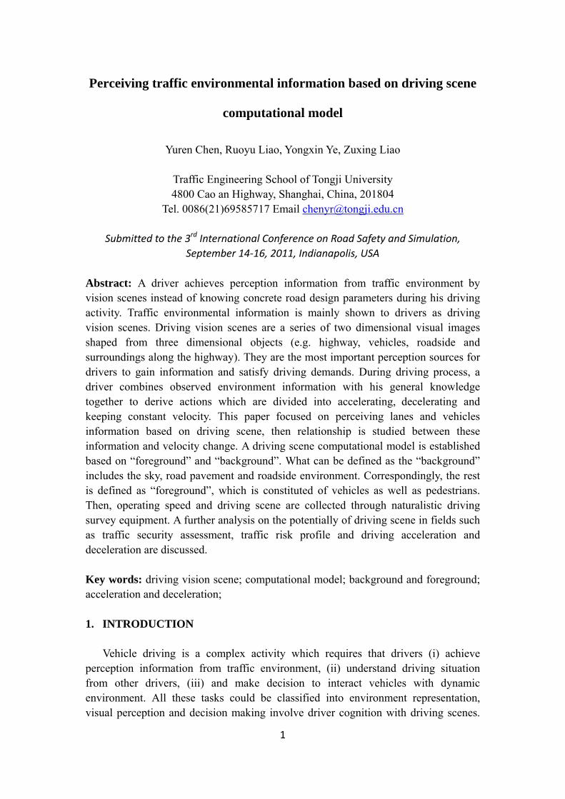
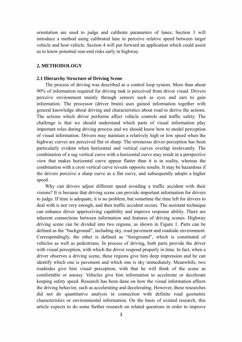
Why can drivers adjust different speed avoiding a traffic accident with their visions? It is because that driving scene can provide important information for drivers to judge. If time is adequate, it is no problem, but sometime the time left for drivers to deal with is not very enough, and then traffic accident occurs. The assistant technique can enhance driver apperceiving capability and improve response ability. There are inherent connections between information and features of driving scenes. Highway driving scene can be divided into two regions, as shown in Figure 1. Parts can be defined as the “background”, including sky, road pavement and roadside environment. Correspondingly, the other is defined as “foreground”, which is constituted of vehicles as well as pedestrians. In process of driving, both parts provide the driver with visual perception, with which the driver respond properly in time. In fact, when a driver observes a driving scene, these regions give him deep impression and he can identify which one is pavement and which one is sky immediately. Meanwhile, two roadsides give him visual perception, with that he will think of the scene as comfortable or uneasy. Vehicles give him information to accelerate or decelerate keeping safety speed. Research has been done on how the visual information affects the driving behavior, such as accelerating and decelerating. However, these researches did not do quantitative analysis in connection with definite road geometric characteristics or environmental information. On the basis of existed research, this article expects to do some further research on related questions in order to improve

4  

computational model of driving scene.

(a) Original image (b) Background image (c) Foreground (d) Focus on lanes & vehicles

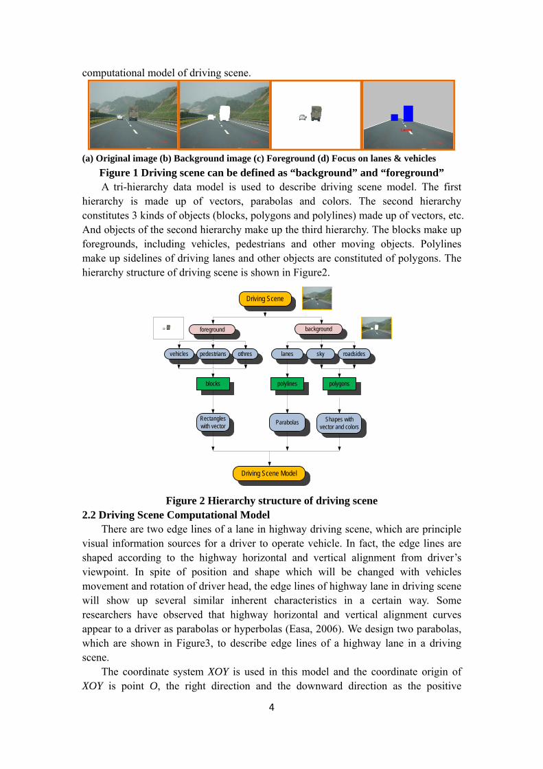
Figure 1 Driving scene can be defined as “background” and “foreground” A tri-hierarchy data model is used to describe driving scene model. The first

hierarchy is made up of vectors, parabolas and colors. The second hierarchy constitutes 3 kinds of objects (blocks, polygons and polylines) made up of vectors, etc. And objects of the second hierarchy make up the third hierarchy. The blocks make up foregrounds, including vehicles, pedestrians and other moving objects. Polylines make up sidelines of driving lanes and other objects are constituted of polygons. The hierarchy structure of driving scene is shown in Figure2.

Figure 2 Hierarchy structure of driving scene 2.2 Driving Scene Computational Model

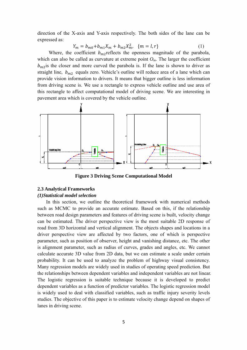
There are two edge lines of a lane in highway driving scene, which are principle visual information sources for a driver to operate vehicle. In fact, the edge lines are shaped according to the highway horizontal and vertical alignment from driver’s viewpoint. In spite of position and shape which will be changed with vehicles movement and rotation of driver head, the edge lines of highway lane in driving scene will show up several similar inherent characteristics in a certain way. Some researchers have observed that highway horizontal and vertical alignment curves appear to a driver as parabolas or hyperbolas (Easa, 2006). We design two parabolas, which are shown in Figure3, to describe edge lines of a highway lane in a driving scene.

The coordinate system XOY is used in this model and the coordinate origin of XOY is point O, the right direction and the downward direction as the positive

Driving Scene

foreground background

lanes sky roadsidesvehicles pedestrians othres

polygons

Shapes with vector and colors

polylinesblocks

Rectangleswith vector Parabolas

Driving Scene Model

5  

direction of the X-axis and Y-axis respectively. The both sides of the lane can be expressed as:

, , (1) Where, the coefficient reflects the openness magnitude of the parabola, which can also be called as curvature at extreme point Om. The larger the coefficient

is the closer and more curved the parabola is. If the lane is shown to driver as straight line, equals zero. Vehicle’s outline will reduce area of a lane which can provide vision information to drivers. It means that bigger outline is less information from driving scene is. We use a rectangle to express vehicle outline and use area of this rectangle to affect computational model of driving scene. We are interesting in pavement area which is covered by the vehicle outline.

Figure 3 Driving Scene Computational Model

2.3 Analytical Frameworks (1)Statistical model selection

In this section, we outline the theoretical framework with numerical methods such as MCMC to provide an accurate estimate. Based on this, if the relationship between road design parameters and features of driving scene is built, velocity change can be estimated. The driver perspective view is the most suitable 2D response of road from 3D horizontal and vertical alignment. The objects shapes and locations in a driver perspective view are affected by two factors, one of which is perspective parameter, such as position of observer, height and vanishing distance, etc. The other is alignment parameter, such as radius of curves, grades and angles, etc. We cannot calculate accurate 3D value from 2D data, but we can estimate a scale under certain probability. It can be used to analyze the problem of highway visual consistency. Many regression models are widely used in studies of operating speed prediction. But the relationships between dependent variables and independent variables are not linear. The logistic regression is suitable technique because it is developed to predict dependent variables as a function of predictor variables. The logistic regression model is widely used to deal with classified variables, such as traffic injury severity levels studies. The objective of this paper is to estimate velocity change depend on shapes of lanes in driving scene.

6  

(2) Independent variables Independent variables are parameters b , b and b , which are estimated

from shapes of lane of driving scene. These parameters should be corrected by position and area of vehicle outline. (3)Classified variables

In this paper, velocity change classifier is a case of ordered. The ordered dependent variables (classifiers categories) might range from 0 to 2, respectively (0 means constant speed, 1 means acceleration and 2 means deceleration). In standard ordered response models, the cumulative probability Pr(X|Y≤k) of velocity change belonging to categories 0 to k is calculated from:

logit (Pr(X|Y≤k))=ln(Pr(X|Y≤k)/(1- Pr(X|Y≤k))= α+βX OR=Pr(X|Y≤k)/(1- Pr(X|Y≤k)) (2)

Where, α is the regression intercept, β is a vector of parameters to be estimated and X is a vector of independent variables ( b , b and b ), k=2. OR is called the odds ratio and it ranges from 0 to positive infinity. If OR is >1, velocity change belongs to categories 0 to k. Cumulative probability Pr(X|Y≤k) is calculated according to the following form formula:

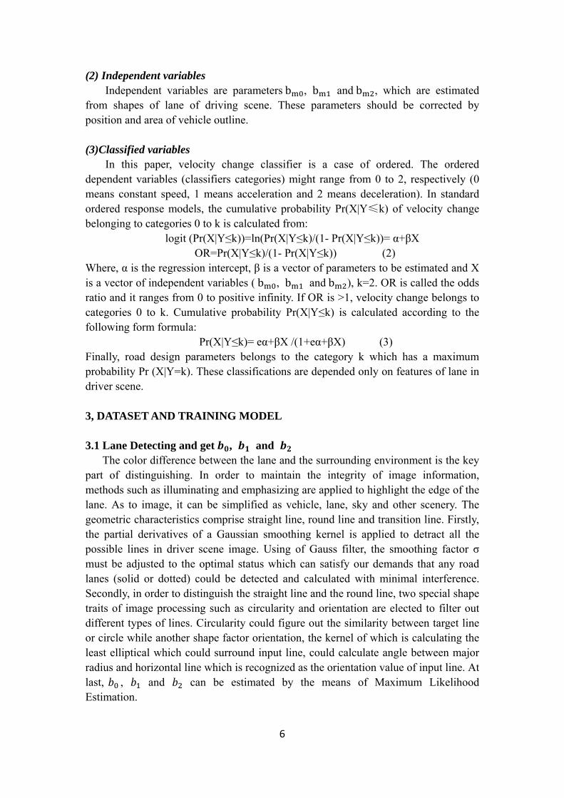
Pr(X|Y≤k)= eα+βX /(1+eα+βX) (3) Finally, road design parameters belongs to the category k which has a maximum probability Pr (X|Y=k). These classifications are depended only on features of lane in driver scene. 3, DATASET AND TRAINING MODEL 3.1 Lane Detecting and get , and

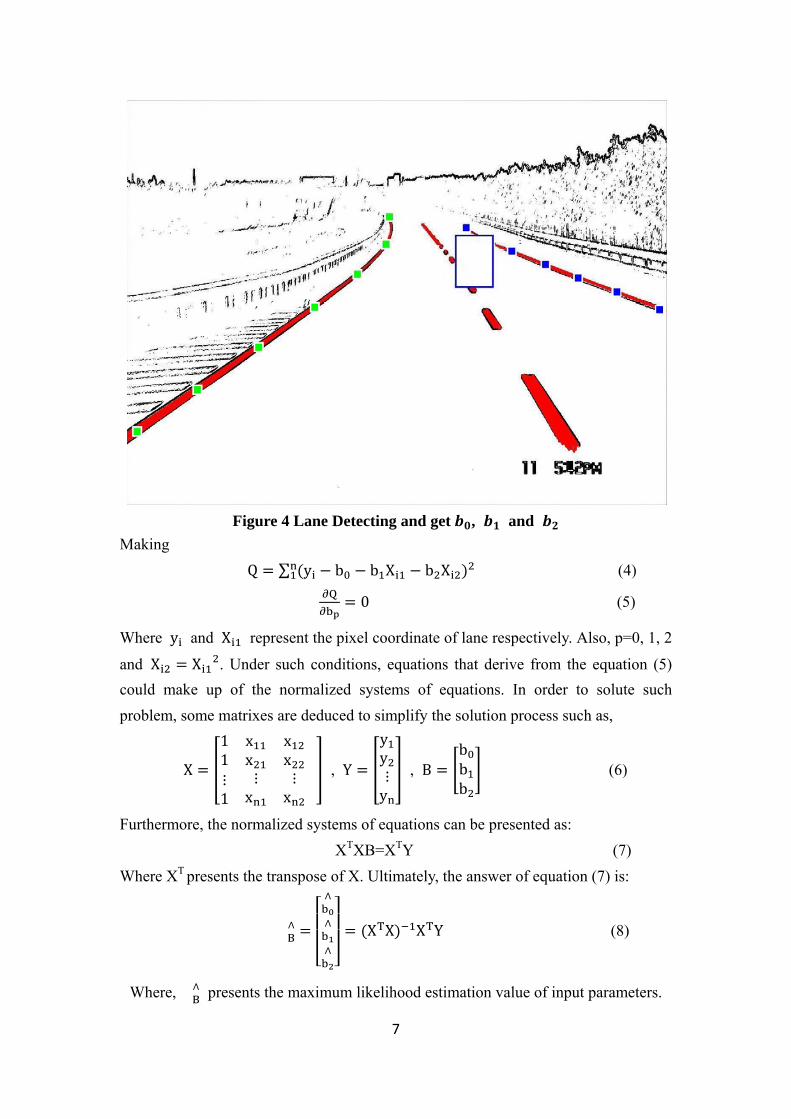
The color difference between the lane and the surrounding environment is the key part of distinguishing. In order to maintain the integrity of image information, methods such as illuminating and emphasizing are applied to highlight the edge of the lane. As to image, it can be simplified as vehicle, lane, sky and other scenery. The geometric characteristics comprise straight line, round line and transition line. Firstly, the partial derivatives of a Gaussian smoothing kernel is applied to detract all the possible lines in driver scene image. Using of Gauss filter, the smoothing factor σ must be adjusted to the optimal status which can satisfy our demands that any road lanes (solid or dotted) could be detected and calculated with minimal interference. Secondly, in order to distinguish the straight line and the round line, two special shape traits of image processing such as circularity and orientation are elected to filter out different types of lines. Circularity could figure out the similarity between target line or circle while another shape factor orientation, the kernel of which is calculating the least elliptical which could surround input line, could calculate angle between major radius and horizontal line which is recognized as the orientation value of input line. At last, , and can be estimated by the means of Maximum Likelihood Estimation.

7  

Figure 4 Lane Detecting and get , and

Making Q ∑ y b b X b X (4)

Q 0 (5)

Where y and X represent the pixel coordinate of lane respectively. Also, p=0, 1, 2

and X X . Under such conditions, equations that derive from the equation (5) could make up of the normalized systems of equations. In order to solute such problem, some matrixes are deduced to simplify the solution process such as,

X

1 x x1 x x

1 x x

, Y

yy

y , B

bbb

(6)

Furthermore, the normalized systems of equations can be presented as: XTXB=XTY (7)

Where XT presents the transpose of X. Ultimately, the answer of equation (7) is:

B XTX XTY (8)

Where, B presents the maximum likelihood estimation value of input parameters.

8  

3.2 Dataset and Training Model

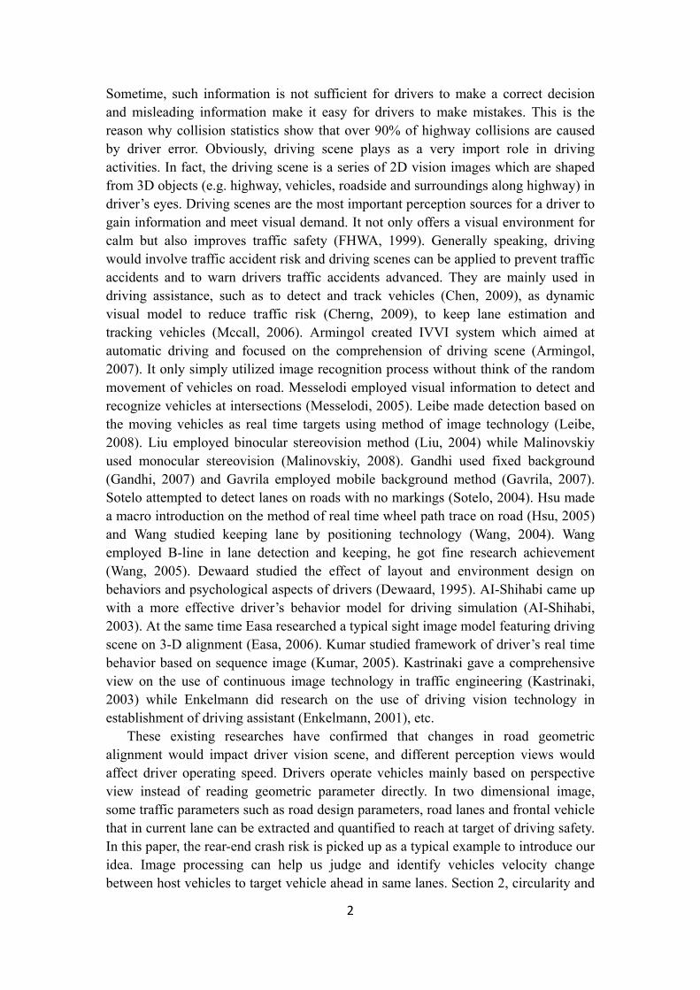
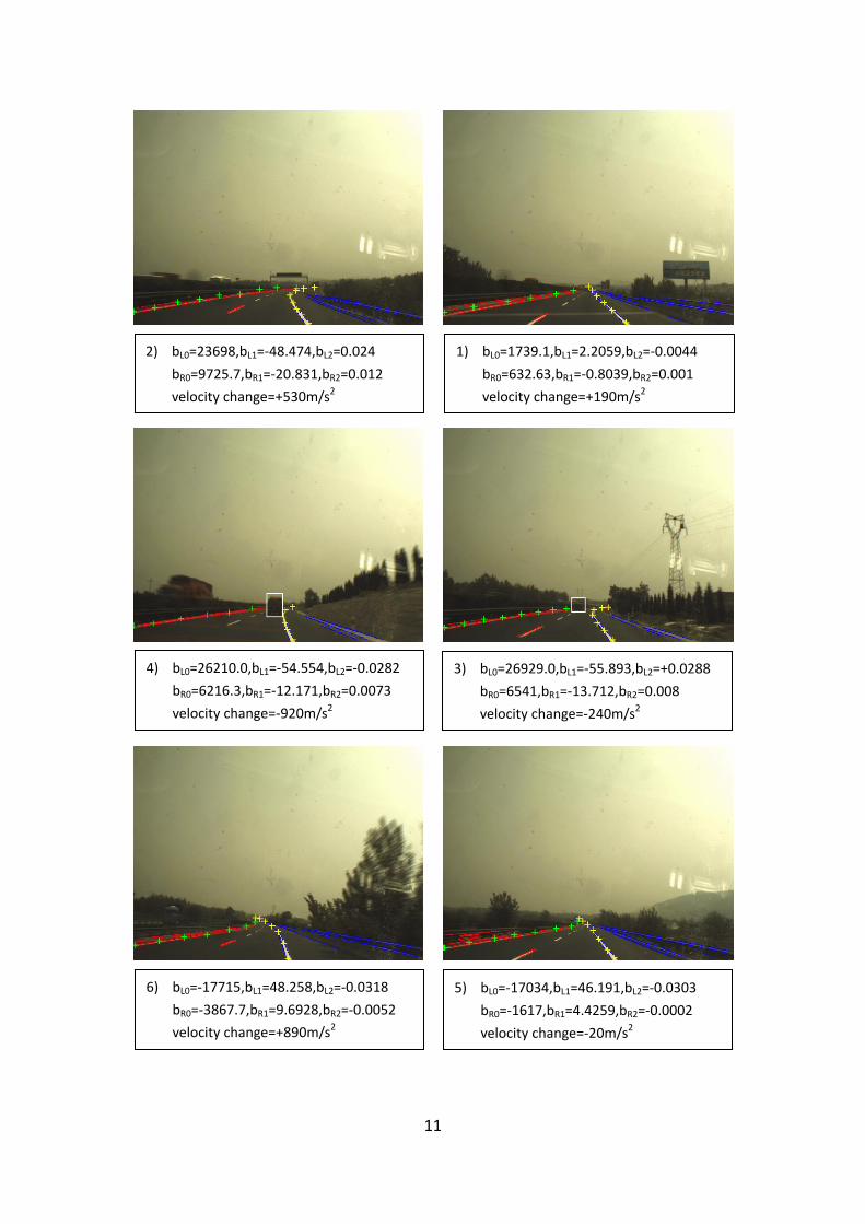
We use a set of digital camera to obtain driving scenes and use a set of GPS to obtain vehicle move velocity. The digital camera is installed behind the windshield so as to cover the similar view angles of the driver. The video of the camera is captured as soon as the vehicle is moving. Strictly speaking, the images acquired by the camera are not entirely representative of driving scene image because of the drivers’ head movement during his driving. But to simplify the experiment, images captured by the camera can be approximated as what the driver actually views. Horizontal alignments contain circular curves, transition curve and tangents. Vertical alignments also contain crest and sag vertical curves which are completely overlapped with horizontal curves. It means that the middle point of vertical curves corresponding to the middle points of horizontal curves as well as the length of each vertical curve equals to the length of corresponding horizontal curve. The values of vertical curvature K (the ratio of vertical curve length to algebraic difference in grade) are distributed along alignment in random. For each group of K, the first grade and second grade of each vertical curve can be calculated. Some examples of dataset and training are shown in figure 5. 4. APPLICATION

As what we have discussed above, there has a strong relationship between driver scene characteristics and velocity change, especially combination of horizontal curves and vertical curves. Meanwhile, eye position of drivers is also an important factor affecting the shape of drivers perspective view. This study could not only help engineers to estimate road design parameters in the practice but also help drivers operate vehicles on the road safely. As a potential technique, it will also assist drivers to scan visual environment that in front of them rapidly during their driving, even may help them to avoid some serious accidents. A pre-warning method, which is based on the visual perception, is discussed in that paper. The key point of pre-warning is how to avoid the disturbance around our target vehicle and get the parameters that we need effectively and efficiently. Due to the complex circumstance, the characteristic of robust may be poor. Accordingly, an approach about re-filtering is applied in this paper to refine scale of lanes. The target vehicle can be extracted with the help of features such as symmetry of gray value and vehicle profile. After that, a parameter which can authentically present the real reaction of drivers is needed to evaluate the process of driving. In this paper, distance is chosen as our control parameter, because only satisfying both the traffic efficiency and the body safety can the driving safety be guaranteed. It is because of the complicated driving circumstance and behavior that the accuracy of identification might be affected. Similarly, the environment information that imputed into our brains will also affect the reaction of the drivers. Even a minor change would cause a tremendous alternative. Accordingly, if the image noise can be removed perfectly as well as both the external influences and the controlling regulations which affect our driving behavior can be reduced to a lighter level, the warning system would qualify and quantify the surroundings more objectively and accurately and play its important rule in our future daily life.

9  

5. ACKNOWLEDGEMENTS All of the authors acknowledge the support from National Science Foundation of China (51078270). REFERENCES Al-Shihabi, T. and R. R. Mourant. (2003). "Toward more realistic driving behavior models for autonomous vehicles in driving simulators" Human Performance, Simulation, User Information Systems, and Older Person Safety and Mobility.1843: 41-49. Armingol, J. M., et al. (2007). "IVVI: Intelligent vehicle based on visual information." Robotics and Autonomous Systems 55.12: 904-16. Chen, Y. L., et al. (2009). "Real-Time Vision-Based Vehicle Detection and Tracking on a Moving Vehicle for Nighttime Driver Assistance." International Journal of Robotics & Automation 24.2: 89-102. Cherng, S., et al. (2009). "Critical Motion Detection of Nearby Moving Vehicles in a Vision-Based Driver-Assistance System." IEEE Transactions on Intelligent Transportation Systems 10.1: 70-82. Dewaard, D., et al. (1995). "Effect of Road Layout and Road Environment on Driving Performance, Drivers Physiology and Road Appreciation." Ergonomics 38.7: 1395-407. Easa, S. M. and W. L. He. (2006). "Modeling driver visual demand on three dimensional highway alignments" Journal of Transportation Engineering ASCE 132.5: 357-65. Enkelmann, W. (2001). "Video-based driver assistance-from basic functions to applications." International Journal of Computer Vision 45.3: 201-21. FHWA. (1999)．"Byways Beginnings: Understanding, Inventorying, and Evaluating a Byway’s Intrinsic Qualities." National Scenic Byways Program Publication. Washington, D.C. Gandhi, T. and M. M. Trivedi. (2007). "Pedestrian protection systems: Issues, survey, and challenges." IEEE Transactions on Intelligent Transportation Systems 8.3: 413-30. Gavrila, D. M. and S. Munder. (2007). "Multi-cue pedestrian detection and tracking from a moving vehicle." International Journal of Computer Vision 73.1: 41-59. Hsu, W. L., et al. (2005). "Real-time vehicle tracking on a highway." Journal of Information Science and Engineering 21.4: 733-52. Kastrinaki, V., M. Zervakis, and K. Kalaitzakis. (2003). "A survey of video processing techniques for traffic applications." Image and Vision Computing, 21.4: 359-81. Kumar, P., et al. (2005). "Framework for real-time behavior interpretation from traffic video." IEEE Transactions on Intelligent Transportation Systems, 6.1: 43-53. Leibe, B., et al. (2008). "Coupled object detection and tracking from static cameras and moving vehicles." IEEE Transactions on Pattern Analysis and Machine Intelligence 30.10: 1683-98.

10  

Liu, X. and K. Fujimura. (2004). "Pedestrian detection using stereo night vision" IEEE Transactions on Vehicular Technology 53.6: 1657-65. Malinovskiy, Y., Y. J. Wu, and Y. H. Wang. (2008). "Video-based Monitoring of Pedestrian Movements at Signalized Intersections." Transportation Research Record.2073: 11-17. Mccall, J. C. and M. M. Trivedi. (2006). "Video-based lane estimation and tracking for driver assistance: Survey, system, and evaluation." IEEE Transactions on Intelligent Transportation Systems 7.1: 20-37. Messelodi, S., C. M. Modena, and M. Zanin. (2005). "A computer vision system for the detection and classification of vehicles at urban road intersections." Pattern Analysis and Applications 8.1-2: 17-31. Sotelo, M. A., et al. (2004). "A color vision-based lane tracking system for autonomous driving on unmarked roads." Autonomous Robots 16.1: 95-116. Wang, Y., E. K. Teoh, and D. G. Shen. (2004). "Lane detection and tracking using B-Snake" Image and Vision Computing 22.4: 269-80. Wang, J., et al. (2005). "Lane keeping based on location technology." IEEE Transactions on Intelligent Transportation Systems 6.3: 351-56.

11  

1) bL0=1739.1,bL1=2.2059,bL2=‐0.0044   

bR0=632.63,bR1=‐0.8039,bR2=0.001   

velocity change=+190m/s2 

2) bL0=23698,bL1=‐48.474,bL2=0.024   

bR0=9725.7,bR1=‐20.831,bR2=0.012   

velocity change=+530m/s2 

4) bL0=26210.0,bL1=‐54.554,bL2=‐0.0282   

bR0=6216.3,bR1=‐12.171,bR2=0.0073   

velocity change=‐920m/s2 

3) bL0=26929.0,bL1=‐55.893,bL2=+0.0288   

bR0=6541,bR1=‐13.712,bR2=0.008   

velocity change=‐240m/s2 

6) bL0=‐17715,bL1=48.258,bL2=‐0.0318   

bR0=‐3867.7,bR1=9.6928,bR2=‐0.0052   

velocity change=+890m/s2 

5) bL0=‐17034,bL1=46.191,bL2=‐0.0303   

bR0=‐1617,bR1=4.4259,bR2=‐0.0002   

velocity change=‐20m/s2 

12  

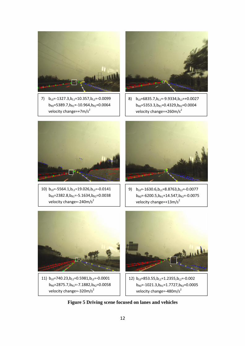
Figure 5 Driving scene focused on lanes and vehicles

7) bL0=‐1327.3,bL1=10.357,bL2=‐0.0099   

bR0=5389.7,bR1=‐10.964,bR2=0.0064   

velocity change=+7m/s2 

8) bL0=6835.7,bL1=‐9.9334,bL2=+0.0027   

bR0=5353.3,bR1=0.4329,bR2=0.0004   

velocity change=+260m/s2 

10) bL0=‐5564.1,bL1=19.026,bL2=‐0.0141   bR0=2382.8,bR1=‐5.1634,bR2=0.0038   

velocity change=‐240m/s2 

9) bL0=‐1630.6,bL1=8.8763,bL2=‐0.0077   

bR0=‐6200.5,bR1=14.547,bR2=‐0.0075   

velocity change=+13m/s2 

11) bL0=740.23,bL1=0.5981,bL2=‐0.0001   bR0=2875.7,bR1=‐7.1882,bR2=0.0058   

velocity change=‐320m/s2 

12) bL0=853.55,bL1=1.2355,bL2=‐0.002   bR0=‐1021.3,bR1=1.7727,bR2=0.0005   

velocity change=‐480m/s2