Pension in The News - Atlanta Actuarial Club

Ozarks Isoprene Experiment (OZIE): Measurements and modeling of

the ‘‘isoprene volcano’’

Christine Wiedinmyer,1 Jim Greenberg,1 Alex Guenther,1 Brian Hopkins,2

Kirk Baker,3 Chris Geron,4 Paul I. Palmer,5 Bryan P. Long,6,7 Jay R. Turner,6

Gabrielle Petron,1 Peter Harley,1 Thomas E. Pierce,4,8 Brian Lamb,2 Hal Westberg,2

William Baugh,1,9 Mike Koerber,3 and Mark Janssen3

Received 25 January 2005; revised 24 June 2005; accepted 20 July 2005; published 24 September 2005.

[1] The Ozarks Isoprene Experiment (OZIE) was conducted in July 1998 in Missouri,Illinois, Indiana, and Oklahoma. OZIE was designed to investigate the presumed strongisoprene emission rates from the Missouri Ozarks, where there is a high density ofoak trees that are efficient isoprene emitters. Ground, balloon, and aircraft measurementswere taken over a three-week study period; 0-D and 3-D chemical models weresubsequently used to better understand the observed isoprene emissions from the Ozarksand to investigate their potential regional-scale impacts. Leaf-level measurements for twooak tree species yielded normalized average isoprene emission capacities of 66 mgC g�1

h�1, in good agreement with values used in current biogenic emissions models. However,the emission capacities exhibited a temperature dependence that is not captured bycommonly used biogenic emission models. Isoprene mixing ratios measured aloft fromtethered balloon systems were used to estimate isoprene fluxes. These measurement-derived fluxes agreed with BEIS3 estimates within the relatively large uncertainties in theestimates. Ground-level isoprene mixing ratios exhibited substantial spatial heterogeneity,ranging from <1 to 35 ppbv. The agreement between measured isoprene mixing ratios andregional-scale chemical transport model estimates was improved upon averaging theground-level isoprene data observed at several sites within a representative area. Ground-level formaldehyde (HCHO) mixing ratios were very high (up to 20 ppbv) and wereconsistently higher than mixing ratios predicted by a regional chemical transport model.The spatial distribution and magnitude of the elevated HCHO concentrations showed goodagreement with GOME satellite column observations of HCHO.

Citation: Wiedinmyer, C., et al. (2005), Ozarks Isoprene Experiment (OZIE): Measurements and modeling of the ‘‘isoprene

volcano,’’ J. Geophys. Res., 110, D18307, doi:10.1029/2005JD005800.

1. Introduction

[2] Isoprene (C5H8) is emitted in significant amountsfrom terrestrial vegetation. The geographic focus of this

paper is North America where the temperate forests of thecentral and eastern United States produce a large fraction ofthe total continental isoprene emissions. The role of iso-prene chemistry in tropospheric ozone (O3) production iswell understood [e.g., Fehsenfeld et al., 1992], but themagnitude and spatiotemporal variability of isoprene emis-sions are uncertain. Ambient concentrations of troposphericO3 have implications for oxidant chemistry in the tropo-sphere, air quality, and climate. Formaldehyde (HCHO), amajor product of isoprene oxidation, can affect the atmo-spheric HOx balance and further contribute to the produc-tion of O3. As a result of this chemistry, isoprene and itsoxidation products impact regional and global air quality.On a regional scale, a better understanding and quantifica-tion of isoprene emissions will improve evaluations of O3

abatement strategies for several regions throughout theUnited States [e.g., Chameides et al., 1988].[3] Current biogenic emissions models such as the Bio-

genic Emissions Inventory System (BEIS) [Pierce andWaldruff, 1991; Lamb et al., 1993; Pierce et al., 1998]predict particularly high isoprene emissions for the oak

JOURNAL OF GEOPHYSICAL RESEARCH, VOL. 110, D18307, doi:10.1029/2005JD005800, 2005

1Atmospheric Chemistry Division, National Center for AtmosphericResearch, Boulder, Colorado, USA.

2Department of Civil and Environmental Engineering, WashingtonState University, Pullman, Washington, USA.

3Lake Michigan Air Directors Consortium, Des Plaines, Illinois, USA.4U.S. Environmental Protection Agency, Research Triangle Park, North

Carolina, USA.5Division of Engineering and Applied Sciences, Harvard University,

Cambridge, Massachusetts, USA.6Department of Chemical Engineering, Washington University, St.

Louis, Missouri, USA.7Now at U.S. Department of Defense, Washington, D. C., USA.8Atmospheric Sciences Modeling Division, National Oceanic and

Atmospheric Administration, Research Triangle Park, North Carolina,USA.

9Now at Hydrobio Consulting, Santa Fe, New Mexico, USA.

Copyright 2005 by the American Geophysical Union.0148-0227/05/2005JD005800$09.00

D18307 1 of 17

forests of the Ozarks in the central United States. Theisoprene emission rates predicted by BEIS3 (http://www.epa.gov/asmdnerl/biogen.html) and using the BELD3 landuse data set [Kinnee et al., 1997, 2005] at a 12 kmresolution for a model domain in the Midwestern UnitedStates are shown in Figure 1. The circled area in thesouthwest corner of the domain identifies the so-called‘‘isoprene volcano,’’ an area of elevated isoprene emissionsthat is predicted for the Missouri Ozarks. Initial modelevaluations of these emissions predicted by BEIS2 sug-gested that these estimates were too high [MoDNR, 1999].However, there were no previous measurements of isopreneemissions in this region with which to evaluate the modeloutput.[4] Although these Midwestern forests emit large

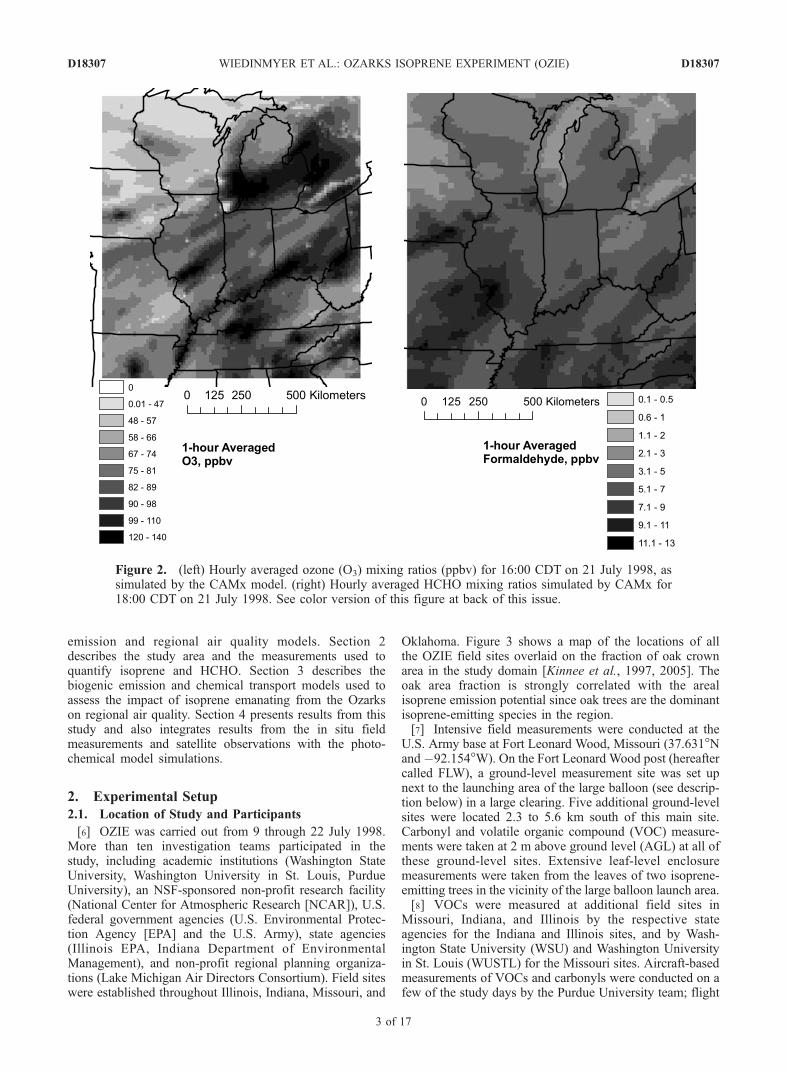
amounts of isoprene, the region is characterized by rela-tively low emissions of oxides of nitrogen, or NOx, and thelocal O3 production from isoprene and NOx chemistry istherefore expected to be small: there may even be a net lossof O3 due to isoprene photochemistry. However, undertypical summertime conditions, the emitted isoprene andits reaction products can be transported northward andeastward to more polluted urban areas such as St. Louisand Chicago. Simulations from a three-dimensional photo-chemical transport model that was used to investigatepotential pollution control strategies for these urban areassuggested that the large isoprene emissions from the Ozarksmay contribute to the O3 burden in these populated areas(Figure 2). Additionally, HCHO is a high yield product of

isoprene oxidation and also a carcinogen included in the listof air toxics by the Clean Air Act. It has been shown toinfluence urban areas far downwind from isoprene sourcesdue to its atmospheric lifetime. The GOME satellite hasobserved elevated HCHO columns over the central U.S.[Palmer et al., 2003], and these observations have beenlargely attributed to isoprene oxidation.[5] Understanding and quantifying the isoprene emis-

sions from the Ozarks is important for predicting air qualityin the central, and possibly, eastern United States. TheOzarks Isoprene Experiment (OZIE) was performed duringJuly 1998 to address several uncertainties in the biogenicisoprene emission inventories in the central United States.The study spanned four states and investigated geographicregions with a variety of landscapes and isoprene emissionpotentials. Three different measurement platforms wereemployed for the study: ground, tethered balloon, andaircraft. The study was designed to address the followingquestions: (1) Can the isoprene emission capacity (deter-mined at 30�C and incident photosynthetically activeradiation (PAR) of 1000 mmol m�2 s�1) of the dominanttree species in the Ozarks be considered constant on timescales of days to weeks, or does it change?, (2) What isthe magnitude of biogenic isoprene emissions from theOzarks?, and (3) How well do emission and chemistrymodels predict the observed isoprene emission rates andatmospheric mixing ratios of isoprene and its oxidationproducts? This paper presents data collected as part of theOZIE study, which can be used for validating isoprene

Figure 1. BEIS3-estimated isoprene emissions for 20 July 1998 at 14:00 CDT. The grid cell size is12 km by 12 km. The oak forests of the Missouri Ozarks are predicted to be a zone of relatively highisoprene emissions (southwestern corner of map) (10,000 gmol h�1 grid cell�1 = 4.72 mg h�1 m�2). Seecolor version of this figure at back of this issue.

D18307 WIEDINMYER ET AL.: OZARKS ISOPRENE EXPERIMENT (OZIE)

2 of 17

D18307

emission and regional air quality models. Section 2describes the study area and the measurements used toquantify isoprene and HCHO. Section 3 describes thebiogenic emission and chemical transport models used toassess the impact of isoprene emanating from the Ozarkson regional air quality. Section 4 presents results from thisstudy and also integrates results from the in situ fieldmeasurements and satellite observations with the photo-chemical model simulations.

2. Experimental Setup

2.1. Location of Study and Participants

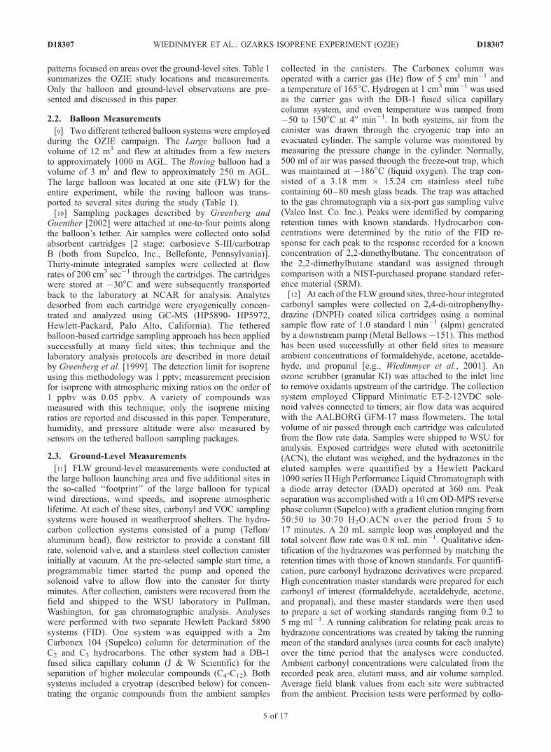
[6] OZIE was carried out from 9 through 22 July 1998.More than ten investigation teams participated in thestudy, including academic institutions (Washington StateUniversity, Washington University in St. Louis, PurdueUniversity), an NSF-sponsored non-profit research facility(National Center for Atmospheric Research [NCAR]), U.S.federal government agencies (U.S. Environmental Protec-tion Agency [EPA] and the U.S. Army), state agencies(Illinois EPA, Indiana Department of EnvironmentalManagement), and non-profit regional planning organiza-tions (Lake Michigan Air Directors Consortium). Field siteswere established throughout Illinois, Indiana, Missouri, and

Oklahoma. Figure 3 shows a map of the locations of allthe OZIE field sites overlaid on the fraction of oak crownarea in the study domain [Kinnee et al., 1997, 2005]. Theoak area fraction is strongly correlated with the arealisoprene emission potential since oak trees are the dominantisoprene-emitting species in the region.[7] Intensive field measurements were conducted at the

U.S. Army base at Fort Leonard Wood, Missouri (37.631�Nand�92.154�W). On the Fort Leonard Wood post (hereaftercalled FLW), a ground-level measurement site was set upnext to the launching area of the large balloon (see descrip-tion below) in a large clearing. Five additional ground-levelsites were located 2.3 to 5.6 km south of this main site.Carbonyl and volatile organic compound (VOC) measure-ments were taken at 2 m above ground level (AGL) at all ofthese ground-level sites. Extensive leaf-level enclosuremeasurements were taken from the leaves of two isoprene-emitting trees in the vicinity of the large balloon launch area.[8] VOCs were measured at additional field sites in

Missouri, Indiana, and Illinois by the respective stateagencies for the Indiana and Illinois sites, and by Wash-ington State University (WSU) and Washington Universityin St. Louis (WUSTL) for the Missouri sites. Aircraft-basedmeasurements of VOCs and carbonyls were conducted on afew of the study days by the Purdue University team; flight

Figure 2. (left) Hourly averaged ozone (O3) mixing ratios (ppbv) for 16:00 CDT on 21 July 1998, assimulated by the CAMx model. (right) Hourly averaged HCHO mixing ratios simulated by CAMx for18:00 CDT on 21 July 1998. See color version of this figure at back of this issue.


3 of 17

D18307

Figure 3. The locations of the field sites of the OZIE study. The fraction of forest oak crown area (colorscale) from the BELD3 data set is shown for the study region. See color version of this figure at back ofthis issue.

Table 1. Summary of Measurement Platforms, Locations, and Data Collected During the OZIE Studya

Site Name

Ft. LeonardWood (Missouri)

BrownCountyPark

(Indiana)

Morgan MonroeState Park(Illinois)

Giant City(Illinois)

SinkinCreek

(Missouri)Candy WMA(Oklahoma)

Tall Grass(Oklahoma)

WillowSprings

(Missouri)

Latitude 37.631 39.162 39.295 37.614 37.502 36.499 36.753 36.918Longitude �92.154 �86.221 �86.438 �89.180 �91.259 �96.035 �96.333 �92.028YYYYMMDD19980708 V V19980709 B, RB, M, V V, AC, AV V, AC, AV19980710 B, RB, M V V19980711 B, M V19980712 B, M RB, V V V19980713 B, M, V, C RB, V, AC, AV V, AC, AV19980714 B, M, V, C V RB, V19980715 B, RB, M V RB, V19980716 B, RB,M, V, C V, AC, AV19980717 B, M RB19980718 B, M, V, C V, AC, AV V, AC, AV RB19980719 B, M, V, C V, AC, AV V, AC, AV19980720 B, M, V, C V V, AC, AV19980721 B, M V, AC, AV V, AC, AV RB, C, V19980722 V V RB, C, V

aB, Big Balloon; RB, Roving Balloon; V, ground-level VOC sampling; C, ground-level carbonyl measurements; AC, aircraft carbonyl measurements;AV, aircraft VOC measurements; M, meteorological measurements.


4 of 17

D18307

patterns focused on areas over the ground-level sites. Table 1summarizes the OZIE study locations and measurements.Only the balloon and ground-level observations are pre-sented and discussed in this paper.

2.2. Balloon Measurements

[9] Two different tethered balloon systems were employedduring the OZIE campaign. The Large balloon had avolume of 12 m3 and flew at altitudes from a few metersto approximately 1000 m AGL. The Roving balloon had avolume of 3 m3 and flew to approximately 250 m AGL.The large balloon was located at one site (FLW) for theentire experiment, while the roving balloon was trans-ported to several sites during the study (Table 1).[10] Sampling packages described by Greenberg and

Guenther [2002] were attached at one-to-four points alongthe balloon’s tether. Air samples were collected onto solidabsorbent cartridges [2 stage: carbosieve S-III/carbotrapB (both from Supelco, Inc., Bellefonte, Pennsylvania)].Thirty-minute integrated samples were collected at flowrates of 200 cm3 sec�1 through the cartridges. The cartridgeswere stored at �30�C and were subsequently transportedback to the laboratory at NCAR for analysis. Analytesdesorbed from each cartridge were cryogenically concen-trated and analyzed using GC-MS (HP5890- HP5972,Hewlett-Packard, Palo Alto, California). The tetheredballoon-based cartridge sampling approach has been appliedsuccessfully at many field sites; this technique and thelaboratory analysis protocols are described in more detailby Greenberg et al. [1999]. The detection limit for isopreneusing this methodology was 1 pptv; measurement precisionfor isoprene with atmospheric mixing ratios on the order of1 ppbv was 0.05 ppbv. A variety of compounds wasmeasured with this technique; only the isoprene mixingratios are reported and discussed in this paper. Temperature,humidity, and pressure altitude were also measured bysensors on the tethered balloon sampling packages.

2.3. Ground-Level Measurements

[11] FLW ground-level measurements were conducted atthe large balloon launching area and five additional sites inthe so-called ‘‘footprint’’ of the large balloon for typicalwind directions, wind speeds, and isoprene atmosphericlifetime. At each of these sites, carbonyl and VOC samplingsystems were housed in weatherproof shelters. The hydro-carbon collection systems consisted of a pump (Teflon/aluminum head), flow restrictor to provide a constant fillrate, solenoid valve, and a stainless steel collection canisterinitially at vacuum. At the pre-selected sample start time, aprogrammable timer started the pump and opened thesolenoid valve to allow flow into the canister for thirtyminutes. After collection, canisters were recovered from thefield and shipped to the WSU laboratory in Pullman,Washington, for gas chromatographic analysis. Analyseswere performed with two separate Hewlett Packard 5890systems (FID). One system was equipped with a 2mCarbonex 104 (Supelco) column for determination of theC2 and C3 hydrocarbons. The other system had a DB-1fused silica capillary column (J & W Scientific) for theseparation of higher molecular compounds (C4-C12). Bothsystems included a cryotrap (described below) for concen-trating the organic compounds from the ambient samples

collected in the canisters. The Carbonex column wasoperated with a carrier gas (He) flow of 5 cm3 min�1 anda temperature of 165�C. Hydrogen at 1 cm3 min�1 was usedas the carrier gas with the DB-1 fused silica capillarycolumn system, and oven temperature was ramped from�50 to 150�C at 4� min�1. In both systems, air from thecanister was drawn through the cryogenic trap into anevacuated cylinder. The sample volume was monitored bymeasuring the pressure change in the cylinder. Normally,500 ml of air was passed through the freeze-out trap, whichwas maintained at �186�C (liquid oxygen). The trap con-sisted of a 3.18 mm � 15.24 cm stainless steel tubecontaining 60–80 mesh glass beads. The trap was attachedto the gas chromatograph via a six-port gas sampling valve(Valco Inst. Co. Inc.). Peaks were identified by comparingretention times with known standards. Hydrocarbon con-centrations were determined by the ratio of the FID re-sponse for each peak to the response recorded for a knownconcentration of 2,2-dimethylbutane. The concentration ofthe 2,2-dimethylbutane standard was assigned throughcomparison with a NIST-purchased propane standard refer-ence material (SRM).[12] At each of the FLWground sites, three-hour integrated

carbonyl samples were collected on 2,4-di-nitrophenylhy-drazine (DNPH) coated silica cartridges using a nominalsample flow rate of 1.0 standard l min�1 (slpm) generatedby a downstream pump (Metal Bellows �151). This methodhas been used successfully at other field sites to measureambient concentrations of formaldehyde, acetone, acetalde-hyde, and propanal [e.g., Wiedinmyer et al., 2001]. Anozone scrubber (granular KI) was attached to the inlet lineto remove oxidants upstream of the cartridge. The collectionsystem employed Clippard Minimatic ET-2-12VDC sole-noid valves connected to timers; air flow data was acquiredwith the AALBORG GFM-17 mass flowmeters. The totalvolume of air passed through each cartridge was calculatedfrom the flow rate data. Samples were shipped to WSU foranalysis. Exposed cartridges were eluted with acetonitrile(ACN), the elutant was weighed, and the hydrazones in theeluted samples were quantified by a Hewlett Packard1090 series II High Performance Liquid Chromatograph witha diode array detector (DAD) operated at 360 nm. Peakseparation was accomplished with a 10 cm OD-MPS reversephase column (Supelco) with a gradient elution ranging from50:50 to 30:70 H2O:ACN over the period from 5 to17 minutes. A 20 mL sample loop was employed and thetotal solvent flow rate was 0.8 mL min�1. Qualitative iden-tification of the hydrazones was performed by matching theretention times with those of known standards. For quantifi-cation, pure carbonyl hydrazone derivatives were prepared.High concentration master standards were prepared for eachcarbonyl of interest (formaldehyde, acetaldehyde, acetone,and propanal), and these master standards were then usedto prepare a set of working standards ranging from 0.2 to5 mg ml�1. A running calibration for relating peak areas tohydrazone concentrations was created by taking the runningmean of the standard analyses (area counts for each analyte)over the time period that the analyses were conducted.Ambient carbonyl concentrations were calculated from therecorded peak area, elutant mass, and air volume sampled.Average field blank values from each site were subtractedfrom the ambient. Precision tests were performed by collo-


5 of 17

D18307

cating samplers both at WSU and at several field locations.From these tests, a precision for all the compounds of betterthan 15% was obtained. The collection efficiency, whichlimits the accuracy of the method, is estimated to be 95–100% for the aldehydes and 90–95% for acetone [Shepsonand Sirju, 1995].

2.4. Leaf-Level Measurements

[13] Repeated measurements were made to determine theisoprene emission capacity (defined here as the rate ofisoprene emission at leaf temperature of 30�C and incidentPAR of 1000 mmol m�2 s�1) of sun-lit leaves from twospecies of oak, Quercus marilandica (blackjack oak) andQ. stellata (post oak). A 6 cm2 portion of a leaf was enclosedin a light and temperature controlled cuvette (LI-6400, Li-Cor, Lincoln, Nebraska). Temperature was controlledthermoelectrically and incident light was provided usingan accessory LED light source (LI-6400-2). Air entering thecuvette was scrubbed of isoprene using an activatedcharcoal filter (Supelco, Bellefonte, Pennsylvania) and flowrate was controlled to �660 cm3 min�1. A portion of the airexiting the leaf enclosure was routed through the 1 cm3

sample loop of the chromatograph where isoprene wasseparated isothermally (100�C) on a stainless steelcolumn (2 mm i.d. and 2 m long) packed with Unibeads 3S,60/80 mesh (Alltech Assoc., Deerfield, Illinois). Isoprenewas quantified using a reduction gas detector (RGD2,Trace Analytical, Menlo Park, California) and peakswere integrated using a commercial integrator (Model 3396,Hewlett-Packard, Avondale, Pennsylvania). The analyticalsystem was calibrated several times daily against a standardcylinder containing 24.1 ppbv isoprene referenced to a NISTpropane standard. Details of the analytical system are givenby Greenberg et al. [1993]. All emission capacity measure-ments were made with incident PAR of 1000 mmol m�2 s�1

and a leaf temperature of 30�C. Under these conditions,isoprene concentrations in the air exiting the enclosure werealways greater than 10 ppbv, well above the system detectionlimit of approximately 0.5 ppbv. After measurements werecompleted, each leaf was oven-dried at 60�C for 48 hours andweighed to determine leaf dry mass, and reported rates are inunits of mgC g�1 h�1.

2.5. Ancillary Data

[14] Meteorological data were collected by the U.S. Armyat five 10 m towers located on the Fort Leonard Wood baseand provided additional temperature, winds, solar radiation,and humidity information.

3. Modeling

[15] Several models were used to support data interpre-tation and biogenic emissions model evaluation. Biogenicemissions fluxes were estimated with an existing model(BEIS3) and also with a 0-D box model driven by the fieldmeasurement data. Photochemical transport modeling wasperformed using the Comprehensive Air Quality Modelwith Extensions (CAMx) version 3.02.

3.1. Emissions Modeling

[16] To produce the necessary emissions for input to thethree-dimensional chemical transport model, emissions data

were processed and merged using EMS-2001 [e.g.,Wilkinson et al., 1994; Hogrefe et al., 2003]. This modelwas selected for its ability to efficiently handle the largerequirements of regional and seasonal or daily emissionsprocessing. In addition to extensive quality assurance andcontrol capabilities, EMS-2001 also performs basic emis-sions processes such as chemical speciation, spatial alloca-tion, and temporal allocation. Outputs from EMS-2001included a coordinate-based elevated point source file andgridded emission estimates for low-elevation point, area,motor vehicle, and biogenic sources. The anthropogenicemissions were based on the 1996 National Emission Inven-tory and were allocated to the modeling grids (describedbelow) with EMS-2001. Anthropogenic emissions estimateswere developed for summer weekday, Saturday, and Sunday.[17] The hourly biogenic emissions for each day of the

model episode were estimated within EMS-2001 [e.g.,Wilkinson et al., 1994; Hogrefe et al., 2003], which usedBEIS3 (http://www.epa.gov/asmdnerl/biogen.html) and theBELD3 land use data set [Kinnee et al., 1997, 2005]. TheBELD3 data set includes high resolution (1 km) mapping oftree species distributions throughout the U.S. and wasdeveloped from field data, including the U.S. Forest Inven-tory Analysis. Inputs to the biogenic emissions modelincluded 15 m (AGL) temperature and PAR data. Thetemperature at 15 m was selected for this applicationbecause of its spatial representation of the tree canopy layer,and these estimates were obtained from output from PennState University/NCAR Mesoscale Meteorological model 5version 2 (MM5) (described below). The PAR inputs werebased on gridded satellite estimates, which are availablefrom the University of Maryland as part of the GEWEXContinental Scale International Project (GCIP) SurfaceRadiation Budget (SRB) [Pinker and Laszlo, 1992; Frouinand Pinker, 1995].

3.2. Three-Dimensional Photochemical TransportModel

[18] Photochemical transport modeling for the periodfrom 16 through 22 July 1998 was performed using theComprehensive Air Quality Model with Extensions(CAMx) version 3.02, a publicly available three-dimensionalphotochemistry and transport model (available at http://www.camx.com). The CAMx simulations used the CarbonBond IV (CB4) gas-phase chemistry mechanism withisoprene chemistry updates [Carter, 1996]. This modelhas been used to simulate regional air quality and to supportozone control strategy development in several regionswithin the United States and throughout the world [e.g.,Nobel et al., 2002; Tanaka et al., 2003; Chen et al., 2003;Morris et al., 2004].[19] The CAMx model simulations used a 36 km coarse

grid and a 12 km fine grid, with 1-way nesting (from thecoarse grid to the fine grid). The coarse grid, which coveredmost of the Central and Eastern United States, was selectedto reconcile boundary conditions for the fine grid thatcovered the Upper Midwest region (Figure 1). The coarsegrid contained 78 cells in the X direction and 67 cells in theY direction. The nested 12 km grid contained 101 cells inthe X direction and 110 cells in the Y direction. Both gridswere centered in the Lambert projection at (�90�W, 40�N),with true parallels at 30�N and 60�N. The atmosphere


6 of 17

D18307

between the surface and 4 km AGL was resolved with12 vertical layers. This vertical structure was chosen tocapture the diurnal variations in the boundary layer, wherethe tops of layers 1 through 9 were 31 m, 76 m, 138 m,261 m, 387 m, 514 m, 642 m, 772 m, and 1071 m AGL.[20] Meteorological input data for the photochemical

model simulations were processed using the Penn StateUniversity/NCAR 5th generation Mesoscale Model(MM5) version 2 [Dudhia, 1993; Grell et al., 1994].Important MM5 parameterizations and physics optionsapplied to each grid included the CCM2 radiationscheme, simple ice moisture, Grell cumulus algorithm,and the Blackadar boundary layer option. GCIP NCEPEta model 3-D and surface analysis data (http://dss.ucar.-edu/datasets/ds609.2/) were used to supply MM5 initialand boundary condition information. Surface and 3-Danalysis nudging for temperature and moisture were onlyapplied above the boundary layer; analysis nudging of thewind fields was applied above and below the boundarylayer. The MM5 model simulations used the same pro-jection and grid resolutions as the CAMx modelingdomains described above and applied two-way nestingwith feedbacks between the fine 12 km grid and thecoarse 36 km grid. MM5 was configured with 26 verticallayers to resolve up to approximately 15 km AGL.Surface wind fields, rain fall, and pressure were comparedto archived UNISYS surface data plots to ensureMM5 output captured important synoptic features in theOzark region during the model episode (http://weather.unisys.com/archive/index.html).

4. Results and Discussion

[21] Measurements of meteorological conditions and themixing ratios of isoprene and several carbonyl species weremade at the surface and in the boundary layer from 9through 22 July 1998. The OZIE study area spanned fourstates in the Midwestern United States, with a focus on thedense oak forests of the Missouri Ozarks (Table 1 andFigure 3). CAMx was run for a seven day period from16 through 22 July 1998 with a nested 12 km domain(Figures 1 and 2). The data collected were used to evaluatethe emission estimates and chemical-transport simulationsof the region.

4.1. Meteorological Measurements

[22] Temperature, radiation, and other meteorologicalparameters were continuously measured at FLW. The con-ditions during the study were primarily sunny and humid,with cloudless or partly cloudy skies. Mid-day temperatures(2 m AGL) at this site ranged from 24.3�C to greater than36�C. Nighttime lows ranged from 15.6�C to 24.3�C.Generally, the first part of the study (9–16 July 1998)was characterized by relatively cooler temperatures, fol-lowed by days (18–21 July 1998) with relatively warmtemperatures (Figure 4a). July 14 was the coolest study day,with the mid-day temperature never rising above 26�C, lowsolar radiation intensity, and high relative humidity. Duringthe final days of measurements (18–21 July 1998), after-noon temperatures were typically 3–4 degrees warmer thanthose observed during the earlier days of the study, withaverage afternoon temperatures close to 35�C. This period

also featured the highest solar radiation intensity and lowestrelative humidity of the entire study period.

4.2. Enclosure Measurements

[23] Enclosure measurements were performed on leavesof two oak trees (Quercus stellata [post oak] andQ. marilandica [blackjack oak]) in the vicinity of the largeballoon launch site at FLW. These species were chosen forstudy because they comprise a large fraction of the oakcrown area in the region and are known to be strongemitters of isoprene. All of the measured leaves werelocated on the outer edge of the crown and were consideredto be sun-lit leaves. The same nine leaves were measuredeach day at approximately the same time; four postoak leaves were measured in the morning between10:00–12:00 CDT, while five blackjack oak leaves weremeasured in the afternoon window 12:30–18:00 CDT. Thepost oak leaves were not in full sunlight during theirmeasurement period and this may have impacted the results.[24] Each day, isoprene emission capacities were deter-

mined for each leaf from the enclosure measurements madeat 30�C and 1000 mmol m�2 s�1; for cases in which the LI-6400 was unable to maintain leaf temperature at 30�Cduring the measurement period, the observed emission rateswere normalized to 30�C using the temperature algorithm ofGuenther et al. [1993] (Figure 4b). The average normalizedemission capacities observed in leaves of the post oak andblackjack oak were 65.6 ± 8.7 and 66.2 ± 10.4 mgC g�1 h�1,respectively (Table 2). These values are in good agreementwith the value of 70 mgC g�1 h�1 assigned to these andother North American oak species in current biogenicemission models [e.g., Geron et al., 2001]. However,Figure 4b demonstrates substantial day-to-day variabilityin average normalized isoprene emission capacity over thenine days of observations, with values ranging from 56.4 to86.5 mgC g�1 h�1 for the blackjack oak, and from 47.2 to78.1 mgC g�1 h�1 for the post oak. This type of variabilityhas been observed in other leaf-level studies [e.g., Petron etal., 2001; Geron et al., 2000] and introduces additionaluncertainty into biogenic emission estimates based on leaf-level emission capacities. In those studies, it has beenproposed that an isoprene emission capacity during a givenmeasurement varies in relation to variation in temperatureover the preceding hours or days.[25] Figure 4a depicts the measured air temperatures (2 m

AGL) at the FLW site over the course of this study. Super-imposed on the instantaneous temperature readings are theaverage air temperatures from the 24 hours prior to thestart of the measurement period (10:00 CDT for the postoak; 12:30 CDT for the blackjack oak). The isopreneemission capacities for both the post oak and blackjackoak leaves generally followed these variations in temper-ature and exhibited a minimum in the middle of the study,corresponding to the period of lowest midday temperatures(Figure 4). The overall trends suggest the emission capac-ities for both species increase with increasing middayambient temperature. Other studies have shown that his-torical (lagged) temperature conditions can affect theisoprene emission capacity [Geron et al., 2000; Guentheret al., 1999; Petron et al., 2001; Sharkey et al., 1999]. Thecorrelation between ambient temperatures observed duringthe leaf-level measurement periods and the average of all


7 of 17

D18307

measured isoprene emission capacities was strong, withr2 = 0.64 (Figure 5). We also investigated the influence ofaverage temperature from the preceding 24 hours andfound a strong correlation with the observed emissioncapacities (r2 = 0.58). These data clearly show that thereis a relationship between ambient temperature and isopreneemission capacity; however, isoprene emission capacitymay potentially be affected by several other environmentalvariables (e.g., PAR, humidity, drought). This data set doesnot allow us to examine those factors. Nevertheless, thestrong correlation between emission capacity and eitherthe ambient temperature at the time of measurement or theaverage temperature over the preceding 24 hours stronglysuggests the importance of temperature in explaining day-to-day variations. These data, with other leaf-level data,may be used to develop and evaluate algorithms thatdescribe the influence of ambient temperatures on emis-sion capacities. These relationships could be included in

future emissions models to more accurately estimate bio-genic isoprene emissions for input to photochemical trans-port models.

4.3. Balloon Measurements

[26] Isoprene mixing ratios were measured from thelarge balloon at altitudes up to 1000 m AGL for 13 daysin July 1998 at the FLW site (Table 1). Measured isoprenemixing ratios from the large balloon ranged from below

Figure 4. (a) Measured diurnal temperatures (2 m AGL) at the FLW site during the OZIE study. Themarkers represent the average temperature for the 24-hour period before sampling began on the post oakand blackjack oak leaves each day (10:00 CDT and 12:30 CDT, respectively). (b) Average calculatedemission capacity (mgC g�1 h�1), normalized to 30�C and 1000 mmol m�2 s�1, for each of the twostudied trees. The error bars represent the standard deviation of the daily measurements made from theleaves of each tree. The dashed line is the average measured emission capacity for all measurements:66 mgC g�1 h�1.

Table 2. Results From Leaf Enclosure Measurementsa

Isoprene Emission Capacities, mgC g�1 h�1

Average MedianStandardDeviation Maximum Minimum N

Post Oak 65.6 66.7 8.7 78.3 43.1 20Blackjack Oak 66.2 65.5 10.4 87.5 41.0 46

aThe calculated emission capacities have been normalized to 30�C and1000 mmol m�2 s�1 using algorithms in Guenther et al. [1993].


8 of 17

D18307

the detection limit (approximately 1 pptv) to over 5 ppbv,with daily maximum values observed closest to the surface(<300 m AGL) at early afternoon (from 12:00 –16:00 CDT). The study-averaged isoprene mixing ratios(with their standard deviations) observed over differentaltitude ranges (50–300 m AGL, 300–500 m AGL, 500–700 m AGL, and 700–1000 m AGL) for various time-of-day intervals are shown in Figure 6. The measured isoprenemixing ratios were relatively low early in the day due to lowemission rates. A strong vertical gradient in the isoprenemixing ratios was observed between the ground-level mea-surements (see next section) and the mixed layer measure-ments from the balloon. Higher isoprene mixing ratios wereobserved near the surface, closest to the emissions source.Daytime mixing ratios (�11:00–18:00 CDT) in the bound-ary layer at altitudes between 300 and 1000 m AGL showedsmall but significant gradients that reflected the strength ofmixing in the mixed layer. These gradients ranged fromapproximately 0.5 ppb to 3 ppb between 100 and 950 m(0.6 to 3.5 ppt m�1). As expected, concentrations decreasedwith height indicating a surface source.[27] During the morning hours (between 6:00 and

9:00 CDT), low isoprene mixing ratios (<1 ppb) wereobserved at altitudes >400 m. The presence of isoprene atthis altitude is likely due to isoprene emitted during theprevious day remaining in the residual layer. The tempera-ture and humidity profiles from the tethered balloon systemindicated that the daytime boundary layer did not typicallyreach 400 m until later in the morning. The highest isoprenemixing ratios (Figure 6; orange markers) were observed inthe newly formed nocturnal boundary layer (�200 m AGL)

in the late afternoons (17:00–20:00 CDT); light-dependentisoprene emissions continued until approximately 18:00;ozone reactions with isoprene in the nocturnal boundarylayer would only slowly reduce nighttime isopreneconcentrations.[28] There were significant variations in the measured

isoprene concentrations from day to day associated withvarying meteorological conditions that affected boundarylayer dynamics and emission rates. As noted in the previoussection, ambient temperatures were relatively cool duringthe middle of the study, and the final days were character-ized by relatively warm temperatures. Generally, emissionsof isoprene were expected to be lowest during the coolertime period of the study and then to increase in the final,hotter days of the study [Guenther et al., 1993]. However,there was no apparent relation between measured isoprenemixing ratios aloft and ambient temperatures at the FLWsite. This phenomenon occurs because an increase intemperature results in two offsetting effects, higher isopreneemissions and higher boundary layer height, which resultsin a nearly constant mixed layer isoprene mixing ratio.[29] Isoprene was measured at elevations of 2 and 250 m

AGL at six sites (in addition to FLW) on ten separate daysusing the roving balloon (Table 3). Observed isoprenemixing ratios ranged from <0.1 ppbv to greater than 9 ppbv.The highest isoprene mixing ratios were observed at theSinkin Creek field site, while the lowest isoprene mixingratios were measured at the Candy Wildlife ManagementArea (WMA). This trend corresponded well with the oakcoverage in the BELD3 database that was used to estimatethe isoprene emissions for the chemical transport modeling;

Figure 5. Correlations between average temperatures (�C) measured at 2 m AGL and the averagemeasured isoprene emission capacities (EC; mgC g�1 h�1) from both the blackjack and the post oakleaves. Two temperature correlations with the measured emission capacities are shown: (1) with theaverage temperature at 2 m AGL over the period when the measurements were made (solid diamonds),and (2) with the average temperature at 2 m AGL for the 24 hours before the measurements were made(open circles).


9 of 17

D18307

BELD3 assigns 53% oak coverage at Sinkin Creek and lessthan 3% oak coverage at Candy WMA. Table 3 summarizesthe daytime (primarily mid-day) mixing ratios of isoprene at�250 m AGL and at ground level (<10 m AGL). Asexpected for a compound with a surface emission, bothballoon data sets (large and roving) showed that isoprenemixing ratios were consistently lower at higher altitudes.This demonstrates that the surface mixing ratio cannot beassumed to be representative of the mixing ratio at 250 m.In addition, the large observed variation in this ratio fordifferent sites and meteorological conditions indicates thatassuming a constant ratio will introduce significant uncer-tainties in estimates of isoprene mixing ratios in the daytimemixed layer.

4.4. Ground-Level Carbonyl and VOC Measurements

[30] VOCs and carbonyls were measured at approximately2 m AGL at five locations within FLW (in addition to thelarge balloon launching site). VOCs and carbonyls werealso measured at other field sites on selected days (Table 1).The ground-level measurements of isoprene and selectedcarbonyls for the various OZIE study sites are summarizedin Table 4. The highest single ground-level isoprene mixingratio (35.8 ppbv) was observed at FLW (specifically, siteFLW5) at 18:15 CDT on 20 July 1998. Indeed, all five

ground-level FLW sites exhibited high isoprene mixingratios during this particular sampling day and time(26.3 ppbv average across the five sites). The environmentalconditions corresponding to this sample period includedtemperatures greater than 36�C, with PAR ranging from500 to 900 mmol m�2 s�1. The elevated temperature, and

Figure 6. Summary of all large balloon measurements conducted during the OZIE study, showingvariations with height and hour-of-day. Markers denote the study-average mixing ratios measured at thespecified time (color scale) and within the altitudes denoted by the gray dotted lines above and below themarkers (50–300 m AGL, 300–500 m AGL, 500–700 m AGL, and 700–1000 m AGL); error barsrepresent the standard deviations of those measurements over the course of the study. See color version ofthis figure at back of this issue.

Table 3. Averaged Daily Concentrations of Isoprene Measured

With Cartridges From Ground-Level and From the Roving

Balloon, and the Ratio of Ground Concentration to the Concentra-

tion Measured at 250 m AGLa

Date(YYYYMMDD) Site Name

Isoprene, pptv

Ground(250 m AGL)/

Ground

19980710 FLW (1) 3688 0.9319980712 Brown Country Park 1206 0.9319980713 Morgan Monroe 2004 0.6219980714 Giant City 823 0.3419980716 FLW (2) 1733 0.6119980717 Candy WMA 218 0.8519980718 Tall Grass 1158 0.5119980721 Willow Springs 3597 0.7819980722 Sinkin Creek 7494 0.43aThe two FLW sites are at different locations on the FLW army base.


10 of 17

D18307

corresponding elevated isoprene emissions, could explainthe high surface isoprene mixing ratios.[31] The daytime isoprene mixing ratios measured at

FLW were much higher than other reported values fromwithin the United States. The mean isoprene mixing ratiofrom all daytime measurements made at the ground sites atFLW during OZIE was 10.8 ppbv. Goldan et al. [1995]observed an average mid-day isoprene mixing ratio of6.3 ppbv for a forested site in southwestern Alabama duringJune and July. Apel et al. [2002] measured isoprene mixingratios at a forested site in northern Michigan in July and

reported mean daytime isoprene mixing ratios to be 1.90 ±0.43 ppbv (with daily maximum mixing ratios on the orderof 10 ppbv). Wiedinmyer et al. [2001] measured meanisoprene mixing ratios ranging from 2.4 to 3.0 ppbv at3 different sites in rural areas of central Texas. Althoughthese other studies took place in forested areas withexpected isoprene emissions, none of the reported isoprenemixing ratios had the same magnitude as the measurementsmade during OZIE.[32] The study-average diurnal profile for ground-level

isoprene mixing ratios (Figure 7) reveals that the maxi-mum observed mixing ratios occurred between 18:00–19:00 CDT. There were large spatial and temporal varia-tions in the FLW ground-level observations despite thesesites being in close proximity (within a few kilometers; seeLong [2003] for details). Three-dimensional photochemicaltransport model evaluations using ground-level point mea-surements from a single site must consider such variabilityin the measured concentrations. Indeed, due to localinfluences, a single point measurement may not be suitablefor evaluating chemical transport model output that has aspatial resolution of several kilometers.[33] Mixing ratios of formaldehyde, acetaldehyde, ace-

tone, and propanal are also summarized in Table 4. At allthree sites located in Missouri, mean acetaldehyde mixingratios did not vary significantly, ranging from 2.4 to2.9 ppbv. This was also the case with the observations ofacetone and propanal, where the mean mixing ratios mea-sured at FLW were 1.7 and 0.3 ppbv, respectively. Formal-dehyde concentrations measured at the Missouri field siteswere relatively high, ranging from 5.4 to 20 ppbv. Theseconcentrations were close to values observed in pollutedurban plumes in Houston, Texas.[34] Satellite observations of HCHO columns from the

Global Ozone Monitoring Experiment (GOME) [Chance etal., 2000] have been shown in previous work to beconsistent with in situ HCHO mixing ratio measurements[Palmer et al., 2003]. In particular, they can be used to

Table 4. Isoprene and Carbonyl Mixing Ratios Measured at the

Ground Sites During the OZIE Study

Site Name

GiantCity,Illinois

MorganMonroe,Illinois

Ft. LeonardWood,Missouri

WillowSprings,Missouri

SinkinCreek,Missouri

Percent Oak 7 8 34 16 53VOC:

Dates Sampled 8–24 Jul 8–24 Jul 9–20 Jul 21 Jul 22 JulN 41 23 69 16 17

IsopreneMean, ppbv 6.4 6.4 10.8 15 15Range, ppbv 0.6–15.4 2.4–15.2 1.8–35.8 8.2–27.2 6.6–24.2

Carbonyls:Dates Sampled 13–20 Jul 21 Jul 22 JulN 45 8 7

FormaldehydeMean, ppbv 11.4 14.0 10.5Range, ppbv 5.4–20.2 9.1–16.3 6.1–13.3

AcetaldehydeMean, ppbv 2.8 2.9 2.4Range, ppbv 1.5–4.8 1.4–3.8 1.1–3.3

AcetoneMean, ppbv 1.7 1.7 2.2Range, ppbv 0.5–3.1 1.1–2.4 1.3–2.8

PropanalMean, ppbv 0.3 0.3 0.3Range, ppbv 0.2–0.6 0.2–0.4 0.2–0.8

Figure 7. Study-average isoprene mixing ratios averaged for ground-level measurements at FLW fordifferent time periods. Bars denote the average mixing ratios for all days and all ground-level sites; errorbars represent the maximum and minimum values of the observed mixing ratios.


11 of 17

D18307

relate findings from in situ data to larger spatial scales.Figure 8 shows surface HCHO mixing ratios (16–22 July1998) inferred from the GOME column data assuming anexponentially decaying vertical profile of HCHO mixingratio with a scale height of 1 km. Under that assumption, thesurface HCHO concentration is related linearly to theobserved HCHO column and the scale height. The dataare averaged on a 2 � 2.5 degree grid, a resolutioncomparable to the largest dimension of the GOME pixel(40 � 320 km2) at mid-latitudes. GOME-derived HCHOmixing ratios at this spatial resolution are likely to corre-spond to greater mixing ratios at smaller scales. GOMEshows elevated formaldehyde mixing ratios (up to 10 ppbv)over the Missouri Ozarks and the OZIE study domain,in good agreement with the in situ measured mixing ratiosat ground-level. The study-averaged in situ daytimeformaldehyde mixing ratios ranged from 11.4 ppbv (atFLW) to 14.0 ppbv (at Willow Springs, Missouri). Thesatellite observations also reveal that elevated HCHOmixing ratios persisted over a larger geographic region thanone might have inferred from the spatially confined ground-level measurements.

4.5. Modeling Results and Evaluation

[35] The data collected during the OZIE study were usedto estimate biogenic isoprene fluxes to the atmosphere.These estimates were then compared to the fluxes predictedby the BEIS3 biogenic emissions model. Finally, observed

isoprene and formaldehyde mixing ratios were comparedto values predicted by photochemical transport modelsimulations.[36] The balloon measurements were used to estimate the

isoprene fluxes from the surface vegetation using a simplechemical box model [Guenther et al., 1996], which assumedthat isoprene is removed only through reactions with O3 andOH. These calculations also assumed the average boundarylayer ozone mixing ratio in the region during the day was40 ppbv (measured at the Fort Leonard Wood airport), theOH concentration was 4 � 106 molecules cm�3 (as isrecommended by Chameides et al. [1992] and Guentheret al. [1996]), and an assumed diurnal profile for theboundary layer height with a maximum height of 1500 mat 12:00–14:00 CDT. The vertical profiles of isoprenemixing ratios observed with the large balloon system wereused to estimate the mixed-layer average isoprene mixingratio. The roving balloon system provides mixed-layerobservations only at 250 m. The roving balloon observa-tions of isoprene mixing ratio at 250 m were related to themixed-layer average mixing ratio using the average verticalprofile observed with the large balloon system. This meth-odology has been applied for previous research efforts toreconstruct isoprene fluxes from boundary layer mixingratio measurements [e.g., Guenther et al., 1996; Wiedinmyeret al., 2001]. The uncertainty associated with the appliedOH mixing ratio was assumed to be 50% [Guenther et al.,1996]. Further uncertainties in the box model flux estimateswere due to uncertainties in the applied O3 concentration,the assumed boundary layer height, and the assumption thatthe balloon measurements were representative of concen-trations in a well-mixed boundary layer.[37] The BEIS3 isoprene fluxes tended to over-predict the

isoprene fluxes reconstructed from the field measurementsusing the box model (Figure 9). An uncertainty of 50% onboth flux estimates are represented by the error bars inFigure 9. Each isoprene flux estimate reconstructed from asingle balloon measurement is shown in Figure 9, includingthose estimated with measurements made when the bound-ary layer may not have been well-mixed. The rovingballoon flew to altitudes of 250 m and only one measure-ment within the boundary layer was made. Measurementsfrom this balloon may not always represent mixing ratiosfrom a well-mixed boundary layer, and the single measure-ment prevents an assessment of when the boundary layerwas well-mixed. Additionally, the roving balloon systemwas operated at eight locations between 36.499� and39.295� latitude and 86.221� to 96.333� longitude. BEIS3underestimated isoprene emissions at 3 sites and overesti-mated at 3 sites relative to the balloon estimates. BEIS3estimated a much larger variability in isoprene emissionbetween sites in comparison to the balloon system. A morequantitative comparison is prevented due to the uncertain-ties associated with the box model estimates (e.g., OH andO3 concentrations and boundary layer height) and thedifference in spatial resolutions between the two estimates.The BEIS3 flux estimates were area-averaged values for agrid cell with 12 km horizontal resolution, whereas theestimated fluxes from the balloon measurements were madefrom single points with different footprints. Direct measure-ments of isoprene fluxes, rather than relying on recon-structed fluxes from observed mixing ratios and a box

Figure 8. Surface HCHO concentrations (ppbv) calculatedfrom HCHO column observations (molec cm�2) from theGOME satellite instrument [Chance et al., 2000] during16–22 July 1998, assuming an exponentially decayingvertical profile of HCHO mixing ratio with a scale height of1 km. Data are for 10–12 local time, averaged on a 2 �2.5 degree grid, and for cloud cover <40%. See colorversion of this figure at back of this issue.


12 of 17

D18307

model, would enable a better evaluation of the biogenicemissions model and are recommended for future fieldstudies.[38] Biogenic emissions were estimated using the BEIS3

model algorithms and satellite-derived PAR. These valueswere used as inputs to the CAMx model for a 7-daysimulation for 16–22 July 1998. The isoprene emissionestimates for 14:00 CDT on 20 July 1998 are shown inFigure 1. Large emissions of isoprene were predicted in theMissouri Ozarks, particularly where the FLW and otherMissouri study sites were located.[39] The chemistry and transport simulated with CAMx

were evaluated with comparisons between measured iso-prene mixing ratios to those predicted by the chemicaltransport model. Four of the FLW ground sites were locatedwithin an area encompassed by a single CAMx grid cell.Figure 10 shows the surface mixing ratio of the isoprenemodeled by CAMx for that particular grid cell (line) and theaverage of the ground-level isoprene mixing ratios mea-sured at the four FLW sites located within the model gridcell area (circles). All of the four FLW ground-levelmeasurements for a given time period have been averaged,and the standard deviations in these measurements are

shown by the error bars. The correlation between theaverage of the measured ground isoprene mixing ratiosand the modeled isoprene mixing ratios had an r2 = 0.53.A stronger correlation is not observed due, in part, to thefact that we are comparing simulated concentrations from amodel with 12 km horizontal resolution (in which each gridis assumed to be well-mixed) to the average of severalsingle point measurements that were each influenced bylocal phenomena. The discrepancies between the modeledand measured isoprene mixing ratios may also be the resultof uncertainties in the simulated meteorology, boundarylayer processes, emissions, and chemistry. However, thecomparison showed that the model did a reasonable job atreproducing the ground-level measurements and their diur-nal variations, suggesting the surface isoprene mixing ratiossimulated by this modeling procedure (emissions estimatedby BEIS3, and subsequent mixing ratios simulated byCAMx) was reliable but contains uncertainties. A compar-ison of the model output with data from a single site, ratherthan averaging over all appropriate sites, resulted in a muchweaker correlation (r2 = 0.35).[40] A comparison of the measured and modeled vertical

profiles of isoprene mixing ratios produced a similar result.Figure 11 shows the average of all isoprene mixing ratiosmeasured within the first nine vertical model layers (up to1071 m AGL) and the average of the correspondingmodeled mixing ratios for the same times and location.The average modeled mixing ratios are from the horizontalgrid cell encompassing the area where the four FLW sites(used in the above discussion) were located. The averagemeasured mixing ratio in Layer 1 (up to 31 m AGL) is anaverage of all canister and cartridge measurements madewithin the area of the model grid cell, and the averagemeasured mixing ratios within Layers 2–9 are from thelarge balloon. The error bars represent the standard devia-tion of the mixing ratios at each layer.[41] The modeled and measured mixing ratios show a

similar vertical structure; however, the results suggest thatthe model may overestimate isoprene mixing ratios at lowerelevations (�<500 m AGL). Possible explanations for themeasurement-model differences could be an overestimate ofsurface-layer isoprene emissions at that site and inaccuratevertical mixing within the model. Uncertainties associatedwith this comparison exist as the result of differences in thetemporal resolutions of the model and measurements. Ad-ditionally, the model output represents the average over anentire vertical layer, whereas the balloon measurementrepresents one point at a particular altitude.[42] Although the differences in the spatial and temporal

resolutions of the GOME satellite estimates of boundarylayer HCHO mixing ratios (Figure 8) and the simulatedsurface concentrations of HCHO from CAMx (Figure 2b)prevent a quantitative comparison, a qualitative analysisof the two estimates suggests good agreement. Bothoutputs showed elevated formaldehyde mixing ratiosabove and downwind of the Missouri Ozarks. The elevatedHCHO mixing ratios were observed over large geographicexpanses. Figure 2b shows the CAMx-modeled formalde-hyde for the late afternoon on 21 July when winds werefrom the south south-west. This formaldehyde, presumablyfrom the oxidation of isoprene emitted in the MissouriOzarks, was also observed in the GOME data. The satellite

Figure 9. Isoprene fluxes (mg m�2 h�1) reconstructedfrom observed isoprene mixing ratios versus BEIS3-estimated isoprene emission fluxes: (a) large balloonmeasurements at FLW; and (b) roving balloon measure-ments at various sites. The error bars represent a 50%uncertainty in all sets of estimates.


13 of 17

D18307

showed very high mixing ratios of HCHO throughoutmuch of Illinois.[43] For three different locations in Missouri (Sinkin

Creek, FLW, and Willow Springs), HCHO mixing ratiosmeasured at multiple, nearby ground-level sites were aver-aged and compared to the model predictions (Figure 12).

In all cases, the observed HCHO mixing ratios were greaterthan the modeled surface layer concentrations. Site-specificvariations in the HCHO mixing ratios did not appear toreconcile the differences between the model estimates andthe observations, and the model consistently under-predicted the HCHO mixing ratios in these geographic areas

Figure 10. Measured (markers) and CAMx-modeled (line) isoprene mixing ratios during the OZIEstudy. Measured mixing ratios are reported as the average of all ground-level sites operated at FLW witherror bars representing the standard deviation of these measurements.

Figure 11. Average measured (triangles) and modeled (squares) isoprene mixing ratios for the verticalmodel layers up to �1000 m AGL. The error bars represent the standard deviation of the mixing ratioswithin each model layer for the compared times.


14 of 17

D18307

of elevated isoprene emissions. Due to the many sources ofuncertainties associated with the model simulations, weonly speculate the reason why the model did not comparewell with the measurements. In addition to the uncertaintiesin the simulated meteorology and boundary layer processes,the model under-prediction could potentially be explainedby inaccurate HCHO and other VOC emissions in thesimulations or underestimation of HCHO transported intothe model domain from other regions. Since HCHO isproduced not only via isoprene oxidation but also fromthe oxidation of many other VOCs, it is possible thatincorrect VOC emissions input to the simulation could haveled to underestimated HCHO mixing ratios. Direct biogenicHCHO emissions could have also contributed to theelevated HCHO mixing ratios in this region; however,HCHO exchange between plants and the atmosphereappears to be dependent on ambient HCHO concentrations[e.g., Rottenberger et al., 2004] and given the high ambientHCHO concentrations, HCHO deposition would be morelikely than emission in this region. HCHO could have beentransported into the study region from elsewhere, and thistransport may not have been simulated correctly within the

CAMx model framework. Future study of the mixing ratiosand fluxes of HCHO in the OZIE study area, and in thesurrounding regions, would be useful for constraining theregional chemical transport models.[44] The under-prediction of HCHO could have important

implications in the regional chemical transport modeling ofthe central United States. The CAMx model output pre-dicted large ozone mixing ratios in the urban areas of St.Louis and Chicago, and these results suggested that, forcertain meteorological conditions, reaction products includ-ing HCHO from the oxidation of isoprene emanating fromthe Missouri Ozarks contributed to the ozone-formingchemistry (e.g., Figure 2). The results of this study showedthat this is a possibility, but further measurements in boththe rural and urban areas of the region should be made tobetter constrain the influence of isoprene and its oxidationproducts on the regional ozone chemistry.

5. Conclusions

[45] A field campaign designed to investigate the bio-genic emissions from oak forests of the Missouri Ozarksand their role in regional oxidant chemistry was conductedin the summer of 1998. Measurements of VOCs, includingisoprene and carbonyls, were made from the surface andwithin the boundary layer. These measurements were usedto evaluate the isoprene emission estimates by the BEIS3model. The measurements were also used to evaluate aregional photochemical transport model that is used toassess regional atmospheric chemistry and provide guidancefor designing pollution control strategies in the urban areasof the region.[46] Measured isoprene emission capacities of two pre-

dominant oak tree species showed that current emissioncapacities applied in biogenic emissions models are appro-priate. However, it appeared that ambient temperatures maycontrol isoprene emission capacities in ways that are notcurrently quantified. New algorithms to describe theseprocesses need to be developed and included in futureemissions models.[47] The ground and balloon ambient measurements

showed relatively high mixing ratios of isoprene, corre-sponding to large biogenic fluxes. The measurementsshowed reasonable agreement with the biogenic emissionsmodel and chemical transport model output, which predictan ‘‘isoprene volcano’’ from the Missouri Ozarks. A com-parison with other field measurements of isoprene demon-strate that the oak forests of the Missouri Ozarks are highemitters of isoprene and indeed are much higher than mostother regions throughout the country, confirming that theBEIS3 estimates for this region are correct in predictingelevated isoprene emissions compared to other sites in thecontinental United States. The agreement between measuredisoprene mixing ratios and regional-scale chemical transportmodel estimates was improved upon averaging the ground-level isoprene data observed at several sites within arepresentative area.[48] Formaldehyde, a high yield isoprene oxidation prod-

uct, was observed in the studied region at high mixingratios. Satellite observations of HCHO agreed well withthese ground-level measurements and showed elevatedmixing ratios on a regional scale, suggesting significant

Figure 12. Measured (markers) and CAMx-modeled(line) formaldehyde mixing ratios at three locations duringthe OZIE study. Measured mixing ratios represent theaverage over all ground-level sites within the modeled gridcell with error bars representing the standard deviation ofthese measurements.


15 of 17

D18307

transport of isoprene oxidation products northward andeastward toward urban centers such as St. Louis andChicago where high levels of anthropogenic NOx will affectthe production of tropospheric O3. A photochemical trans-port model appeared to predict this episode of elevatedHCHO, but underpredicted the magnitude of the HCHOmixing ratios in rural regions. This underestimation couldpotentially lead to incorrect chemistry simulations withinthe urban centers of the region. Therefore, it is recommen-ded that further measurements be made in the Midwesternurban centers to identify the accuracy of the model pre-dictions for HCHO and the impact of the isoprene emittedfrom the Ozarks. Furthermore, biogenic emissions and theirreaction products need to be considered more criticallywhen evaluating the atmospheric chemistry in the urbancenters of the Midwest towards determining optimal O3

control strategies.

[49] Acknowledgments. The authors would like to thank the UnitedStates Army – Fort Leonard Wood post, the Illinois EnvironmentalProtection Agency, and the Indiana Department of Environmental Man-agement. Ground-level measurements conducted by Washington StateUniversity and Washington University were funded by the Missouri ElectricUtility Environmental Committee (MEUEC) through M. Kenneth Anderson(AmerenUE). The authors would like to thank the anonymous reviewers ofthis paper for their useful suggestions and comments. Paul I. Palmeracknowledges support from the Atmospheric Chemistry Program of theNational Science Foundation. The National Center for AtmosphericResearch is sponsored by the National Science Foundation.

ReferencesApel, E. C., et al. (2002), Measurement and interpretation of isoprene fluxesand isoprene, methacrolein, and methyl vinyl ketone mixing ratios at thePROPHET site during the 1998 intensive, J. Geophys. Res., 107(D3),4034, doi:10.1029/2000JD000225.

Carter, W. P. L. (1996), Condensed atmospheric photooxidation mecha-nisms for isoprene, Atmos. Environ., 30, 4275–4290.

Chameides, W., R. W. Lindsay, J. Richardson, and C. S. Kiang (1988), Therole of biogenic hydrocarbons in urban photochemical smog - Atlanta asa case study, Science, 241(4872), 1473–1475.

Chameides, W., et al. (1992), Ozone precursor relationships in the ambientatmosphere, J. Geophys. Res., 97, 6037–6055.

Chance, K., P. I. Palmer, R. J. D. Spurr, R. V. Martin, T. P. Kurosu, andD. Jacob (2000), Satellite observations of formaldehyde over NorthAmerica from GOME, Geophys. Res. Lett., 27(21), 3461–3464.

Chen, K. S., Y. T. Ho, C. H. Lai, and Y.-M. Chou (2003), Photochemicalmodeling and analysis of meteorological parameters during ozone epi-sodes in Kaohsiung, Taiwan, Atmos. Environ., 37(13), 1811–1823.

Dudhia, J. (1993), A nonhydrostatic version of the Penn State/NCARmesoscale model: Validation tests and simulation of an Atlantic cycloneand cold front, Mon. Weather Rev., 121, 1493–1513.

Fehsenfeld, F., et al. (1992), Emissions of volatile organic compounds fromvegetation and the implications for atmospheric chemistry, Global Bio-geochem. Cycles, 6(4), 389–430.

Frouin, R., and R. T. Pinker (1995), Estimating Photosynthetically ActiveRadiation (PAR) of the Earth’s surface from satellite observations,Remote Sens. Environ., 51, 98–107.

Geron, C., A. Guenther, T. Sharkey, and R. R. Arnts (2000), Temporalvariability in basal isoprene emission factor, Tree Physiol., 20(12),799–805.

Geron, C., P. Harley, and A. Guenther (2001), Isoprene emission capacityfor U.S. tree species, Atmos. Environ., 35(19), 3341–3352.

Goldan, P. D., W. C. Kuster, F. C. Fehsenfeld, and S. A. Montzka (1995),Hydrocarbon measurements in the southeastern United States: The RuralOxidants in the Southern Environment (ROSE) Program 1990, J. Geo-phys. Res., 100(D12), 25,945–25,963.

Greenberg, J., and A. Guenther (2002), Tethered-balloon profiling for atmo-spheric boundary layer chemistry, in Environmental Monitoring Hand-book, edited by F. B. Burden, I. McKelvie, U. Forstner, and A. Guenther,pp. 20.1–20.14, McGraw-Hill, New York.

Greenberg, J. P., P. R. Zimmerman, B. E. Taylor, G. M. Silver, and R. Fall(1993), Subparts per billion detection of isoprene using a reduction gasdetector with a portable gas chromatograph, Atmos. Environ., 27,2689–2692.

Greenberg, J. P., A. Guenther, P. Zimmerman, W. Baugh, C. Geron,K. Davis, D. Helmig, and L. F. Klinger (1999), Tethered balloonmeasurements of biogenic VOCs in the atmospheric boundary layer,Atmos. Environ., 33(6), 855–867.

Grell, G. A., J. Dudhia, and D. Stauffer (1994), A description of theFifth Generation Penn State/NCAR Mesoscale Model (MM5), NCARTech. Note TN-398-STR, 138 pp., Natl. Cent. for Atmos. Res.,Boulder, Colo.

Guenther, A., P. Zimmerman, P. Harley, R. K. Monson, and R. Fall(1993), Isoprene and monoterpene emission rate variability: Modelevaluations and sensitivity analyses, J. Geophys. Res., 98, 12,609–12,617.

Guenther, A., et al. (1996), Isoprene fluxes measured by enclosure, relaxededdy accumulation, surface layer gradient, mixed layer gradient, andmixed layer mass balance techniques, J. Geophys. Res., 101(D13),18,555–18,567.

Guenther, A., B. Baugh, G. Brasseur, J. Greenberg, P. Harley, L. Klinger,D. Serca, and L. Vierling (1999), Isoprene emission estimates and uncer-tainties for the Central African EXPRESSO study domain, J. Geophys.Res., 104, 30,625–30,639.

Hogrefe, C., G. Sistla, E. Zalewsky, W. Hao, and J.-Y. Ku (2003), Anassessment of the emissions inventory processing systems EMS-2001and SMOKE in grid-based air quality models, J. Air Waste Manage.Assoc., 53(9), 1121–1129.

Kinnee, E., C. Geron, and T. Pierce (1997), United States land use inven-tory for estimating biogenic ozone precursor emissions, Ecol. Appl., 7(1),46–58.

Kinnee, E., C. Geron, and T. Pierce (2005), Development of a 1-km re-solved vegetation database for surface exchange modeling in NorthAmerica, Ecol. Appl., in press.

Lamb, B., D. Gay, H. Westberg, and T. Pierce (1993), A biogenic hydro-carbon emission inventory for the U.S. using a simple forest canopymodel, Atmos. Environ., 27(11), 1673–1690.

Long, B. (2003), The Ozark Isoprene Experiment: A study of biogenicemissions within the Ozark Forest, Missouri, M.S. thesis, Environ.Eng. Program, Washington Univ., St. Louis, Mo., Dec.

MoDNR (1999), Missouri Air Quality Control Plan, Mo. Dep. of Nat.Resour., Jefferson City, Mo.

Morris, R. E., G. Mansell, and E. Tai (2004), Air quality modeling analysisfor the Denver Early Action Ozone Compact, Denver Reg. Air Qual.Counc., Denver, Colo.

Nobel, C. E., E. C. McDonald-Buller, Y. Kimura, K. E. Lumbley, and D. T.Allen (2002), Influence of population density and temporal variations inemissions on the air quality benefits of NOx emission trading, Environ.Sci. Technol., 36, 3465–3473.

Palmer, P. I., D. J. Jacob, A. M. Fiore, R. V. Martin, K. Chance, and T. P.Kurosu (2003), Mapping isoprene emissions over North America usingformaldehyde column observations from space, J. Geophys. Res.,108(D6), 4180, doi:10.1029/2002JD002153.

Petron, G., P. Harley, J. Greenberg, and A. Guenther (2001), Seasonaltemperature variations influence isoprene emission, Geophys. Res. Lett.,28(9), 1707–1710.

Pierce, T., and P. S. Waldruff (1991), Pc-Beis - A personal-computer ver-sion of the Biogenic Emissions Inventory System, J. Air Waste Manage.Assoc., 41(7), 937–941.

Pierce, T., C. Geron, L. Bender, R. Dennis, G. Tonnesen, and A. Guenther(1998), Influence of increased isoprene emissions on regional ozonemodeling, J. Geophys. Res., 103(D19), 25,611–25,629.

Pinker, R. T., and I. Laszlo (1992), Modeling surface solar irradiance forsatellite applications on a global scale, J. Appl. Meteorol., 31, 194–211.

Rottenberger, S., U. Kuhn, A. Wolf, G. Schebeske, S. T. Oliva, T. M.Tavares, and J. Kesselmeier (2004), Exchange of short-chain aldehydesbetween Amazonian vegetation and the atmosphere, Ecol. Appl., 14(4),suppl., S247–S262.

Sharkey, T. D., E. L. Singsaas, M. T. Lerdau, and C. D. Geron (1999),Weather effects on isoprene emission capacity and applications in emis-sions algorithms, Ecol. Appl., 9(4), 1132–1137.

Shepson, P. B., and A. P. Sirju (1995), Laboratory and field investigation ofthe DNPH cartridge technique for the measurement of atmospheric car-bonyl compounds, Environ. Sci. Technol., 29, 384–392.

Tanaka, P. L., D. T. Allen, E. C. McDonald-Buller, S. Chang, Y. Kimura,C. B. Mullins, G. Yarwood, and J. D. Neece (2003), Develop-ment of a chlorine mechanism for use in the CAMx regionalphotochemical model, J. Geophys. Res., 108(D4), 4145, doi:10.1029/2002JD002432.

Wiedinmyer, C., S. Friedfeld, W. Baugh, J. Greenberg, A. Guenther,M. Fraser, and D. Allen (2001), Measurement and analysis of atmo-spheric concentrations of isoprene and its reaction products in centralTexas, Atmos. Environ., 35(6), 1001–1013.


16 of 17

D18307

Wilkinson, J., C. Loomis, R. Emigh, D. McNalley, and T. Tesche (1994),Technical formulation document: SARMAP/LMOS Emissions ModelingSystem (EMS-95), final report, Lake Mich. Air Dir. Consortium, DesPlaines, Ill. (EMS-95 User’s Guide available at http://www.ladco.org/emis/guide/ems95.html)

��K. Baker, M. Janssen, and M. Koerber, Lake Michigan Air Directors

Consortium, Des Plaines, IL 60018, USA.W. Baugh, Hydrobio Consulting, 1220 Cerro Gordo Rd., Santa Fe, NM

87501, USA.C. Geron, U.S. Environmental Protection Agency, Research Triangle

Park, NC 27711, USA.

J. Greenberg, A. Guenther, P. Harley, G. Petron, and C. Wiedinmyer,Atmospheric Chemistry Division, National Center for AtmosphericResearch, Boulder, CO 80303, USA. ([email protected])B. Hopkins, B. Lamb, and H. Westberg, Department of Civil and

Environmental Engineering, Washington State University, Pullman, WA99164-5702, USA.B. P. Long, U.S. Department of Defense, Washington, DC 20015, USA.P. I. Palmer, Division of Engineering and Applied Sciences, Harvard

University, Cambridge, MA 02138, USA.T. E. Pierce, Atmospheric Sciences Modeling Division, National Oceanic

and Atmospheric Administration, Research Triangle Park, NC 27711-0001,USA.J. R. Turner, Department of Chemical Engineering, Washington

University, St. Louis, MO 63130, USA.


17 of 17

D18307

Figure 1. BEIS3-estimated isoprene emissions for 20 July 1998 at 14:00 CDT. The grid cell size is12 km by 12 km. The oak forests of the Missouri Ozarks are predicted to be a zone of relatively highisoprene emissions (southwestern corner of map) (10,000 gmol h�1 grid cell�1 = 4.72 mg h�1 m�2).

D18307 WIEDINMYER ET AL.: OZARKS ISOPRENE EXPERIMENT (OZIE) D18307

2 of 17

Figure 2. (left) Hourly averaged ozone (O3) mixing ratios (ppbv) for 16:00 CDT on 21 July 1998, assimulated by the CAMx model. (right) Hourly averaged HCHO mixing ratios simulated by CAMx for18:00 CDT on 21 July 1998.


3 of 17

Figure 3. The locations of the field sites of the OZIE study. The fraction of forest oak crown area (colorscale) from the BELD3 data set is shown for the study region.


4 of 17

Figure 6. Summary of all large balloon measurements conducted during the OZIE study, showingvariations with height and hour-of-day. Markers denote the study-average mixing ratios measured at thespecified time (color scale) and within the altitudes denoted by the gray dotted lines above and below themarkers (50–300 m AGL, 300–500 m AGL, 500–700 m AGL, and 700–1000 m AGL); error barsrepresent the standard deviations of those measurements over the course of the study.


10 of 17

Figure 8. Surface HCHO concentrations (ppbv) calculated from HCHO column observations (moleccm�2) from the GOME satellite instrument [Chance et al., 2000] during 16–22 July 1998, assuming anexponentially decaying vertical profile of HCHO mixing ratio with a scale height of 1 km. Data are for10–12 local time, averaged on a 2 � 2.5 degree grid, and for cloud cover <40%.


12 of 17

Pension in The News - Atlanta Actuarial Club

Documents

Transcript of Pension in The News - Atlanta Actuarial Club