Penn ESE525 Spring 2008 -- DeHon 1 ESE535: Electronic Design Automation Day 10: February 27, 2008...
49
Penn ESE525 Spring 2008 -- DeHo n 1 ESE535: Electronic Design Automation Day 10: February 27, 2008 Partitioning 2 (spectral, network flow, replication)
-
date post
19-Dec-2015 -
Category
Documents
-
view
214 -
download
0
Transcript of Penn ESE525 Spring 2008 -- DeHon 1 ESE535: Electronic Design Automation Day 10: February 27, 2008...

Penn ESE525 Spring 2008 -- DeHon 1
ESE535:Electronic Design Automation
Day 10: February 27, 2008
Partitioning 2
(spectral, network flow, replication)

Penn ESE525 Spring 2008 -- DeHon 2
Today
• Alternate views of partitioning
• Two things we can solve optimally– (but don’t exactly solve our original
problem)
• Techniques– Linear Placement w/ squared wire lengths– Network flow MinCut

Penn ESE525 Spring 2008 -- DeHon 3
Optimization Target
• Place cells
• In linear arrangement
• Wire length between connected cells:– distance=Xi - Xj
– cost is sum of distance squared
Pick Xi’s to minimize cost

Penn ESE525 Spring 2008 -- DeHon 4
Why this Target?
• Minimize sum of squared wire distances
• Prefer:– Area: minimize channel width– Delay: minimize critical path
length
Penn ESE525 Spring 2008 -- DeHon 5
Why this Target?
• Our preferred targets are discontinuous and discrete
• Cannot formulate analytically• Not clear how to drive toward
solution– Does reducing the channel width
at a non-bottleneck help or not?– Does reducing a non-critical path
help or not?

Penn ESE525 Spring 2008 -- DeHon 6
Spectral Ordering
Minimize Squared Wire length -- 1D layout
• Start with connection array C (ci,j)
• “Placement” Vector X for xi placement
• Problem:
– Minimize cost = 0.5* (all i,j) (xi- xj)2 ci,j
– cost sum is XTBX• B = D-C
• D=diagonal matrix, di,i = (over j) ci,j
Penn ESE525 Spring 2008 -- DeHon 7
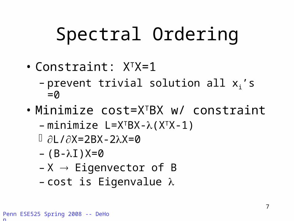
Spectral Ordering
• Constraint: XTX=1– prevent trivial solution all xi’s =0
• Minimize cost=XTBX w/ constraint– minimize L=XTBX-(XTX-1) L/X=2BX-2X=0– (B-I)X=0– X Eigenvector of B– cost is Eigenvalue

Penn ESE525 Spring 2008 -- DeHon 8
Spectral Solution
• Smallest eigenvalue is zero– Corresponds to case where all xi’s are the
same uninteresting
• Second smallest eigenvalue (eigenvector) is the solution we want

Penn ESE525 Spring 2008 -- DeHon 9
Spectral Ordering
• X (xi’s) continuous
• use to order nodes– real problem wants to place at discrete
locations– this is one case where can solve ILP from
LP
• Solve LP giving continuous xi’s
• then move back to closest discrete point
Penn ESE525 Spring 2008 -- DeHon 10
Spectral Ordering Option
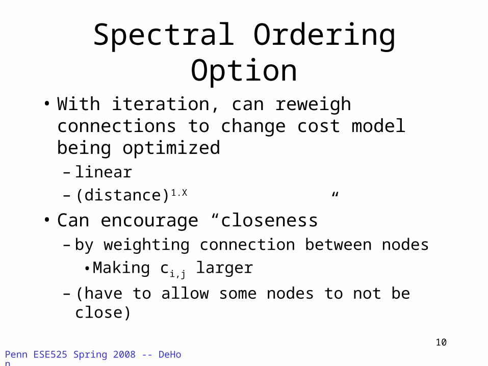
• With iteration, can reweigh connections to change cost model being optimized– linear– (distance)1.X
• Can encourage “closeness”– by weighting connection between nodes
• Making ci,j larger
– (have to allow some nodes to not be close)

Penn ESE525 Spring 2008 -- DeHon 11
Spectral Partitioning
• Can form a basis for partitioning
• Attempts to cluster together connected components
• Form cut partition from ordering– E.g. Left half of ordering is one half, right
half is the other

Penn ESE525 Spring 2008 -- DeHon 12
Spectral Ordering
• Midpoint bisect isn’t necessarily best place to cut, consider:
K(n/4) K(n/4)K(n/2)

Penn ESE525 Spring 2008 -- DeHon 13
Fanout
• How do we treat fanout?
• As described assumes point-to-point nets
• For partitioning, pay price when cut something once– I.e. the accounting did last time for KLFM
• Also a discrete optimization problem– Hard to model analytically

Penn ESE525 Spring 2008 -- DeHon 14
Spectral Fanout
• Typically:– Treat all nodes on a single net as fully
connected– Model links between all of them– Weight connections so cutting in half counts
as cutting the wire– Threshold out high fanout nodes
• If connect to too many things give no information

Penn ESE525 Spring 2008 -- DeHon 15
Spectral Partitioning Options• Can bisect by choosing midpoint
– (not strictly optimizing for minimum bisect)
• Can relax cut critera– min cut w/in some of balance
• Ratio Cut– minimize (cut/|A||B|)
• idea tradeoff imbalance for smaller cut– more imbalance smaller |A||B|– so cut must be much smaller to accept
• Circular bisect/relaxed/ratio cut– wrap into circle and pick two cut points– How many such cuts?

Penn ESE525 Spring 2008 -- DeHon 16
Spectral vs. FM
From Hauck/Boriello ‘96
Penn ESE525 Spring 2008 -- DeHon 17
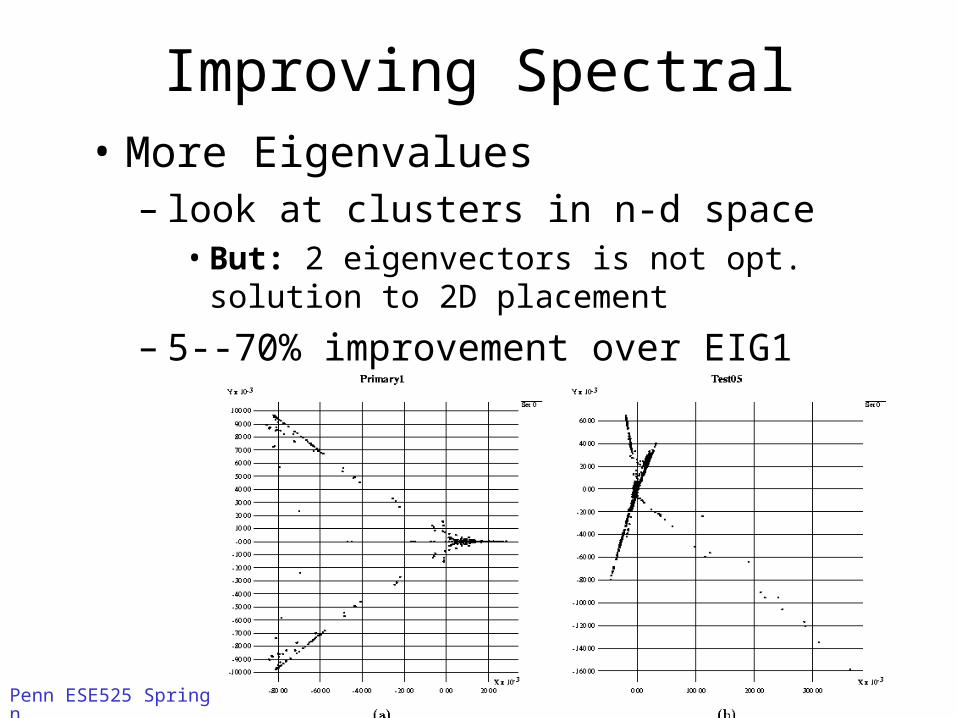
Improving Spectral• More Eigenvalues
– look at clusters in n-d space • But: 2 eigenvectors is not opt. solution to 2D
placement
– 5--70% improvement over EIG1

Penn ESE525 Spring 2008 -- DeHon 18
Spectral Note
• Unlike KLFM, attacks global connectivity characteristics
• Good for finding “natural” clusters– hence use as clustering heuristic for
multilevel algorithms

Penn ESE525 Spring 2008 -- DeHon 21
Max Flow
MinCut

Penn ESE525 Spring 2008 -- DeHon 22
MinCut Goal
• Find maximum flow (mincut) between a source and a sink– no balance guarantee

Penn ESE525 Spring 2008 -- DeHon 23
MaxFlow
• Set all edge flows to zero– F[u,v]=0
• While there is a path from s,t – (breadth-first-search)– for each edge in path f[u,v]=f[u,v]+1– f[v,u]=-f[u,v]– When c[v,u]=f[v,u] remove edge from search
• O(|E|*cutsize)• [Our problem simpler than general case CLR]

Penn ESE525 Spring 2008 -- DeHon 24
Technical Details
• For min-cut in graphs,– Don’t really care about directionality of cut– Just want to minimize wire crossings
• Fanout– Want to charge discretely …cut or not cut
• Pick start and end nodes?
Penn ESE525 Spring 2008 -- DeHon 25
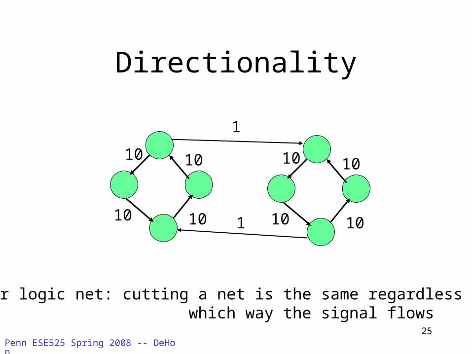
Directionality
10
10
10
10
10
10
10
10
1
1
For logic net: cutting a net is the same regardless of which way the signal flows

Penn ESE525 Spring 2008 -- DeHon 26
Directionality Construct
1

Penn ESE525 Spring 2008 -- DeHon 27
Fanout Construct
1

Penn ESE525 Spring 2008 -- DeHon 28
Extend to Balanced Cut
• Pick a start node and a finish node• Compute min-cut start to finish• If halves sufficiently balanced, done• else
– collapse all nodes in smaller half into one node– pick a node adjacent to smaller half– collapse that node into smaller half– repeat from min-cut computation
FBB -- Yang/Wong ICCAD’94

Penn ESE525 Spring 2008 -- DeHon 29
Observation
• Can use residual flow from previous cut when computing next cuts
• Consequently, work of multiple network flows is only O(|E|*final_cut_cost)
Penn ESE525 Spring 2008 -- DeHon 30
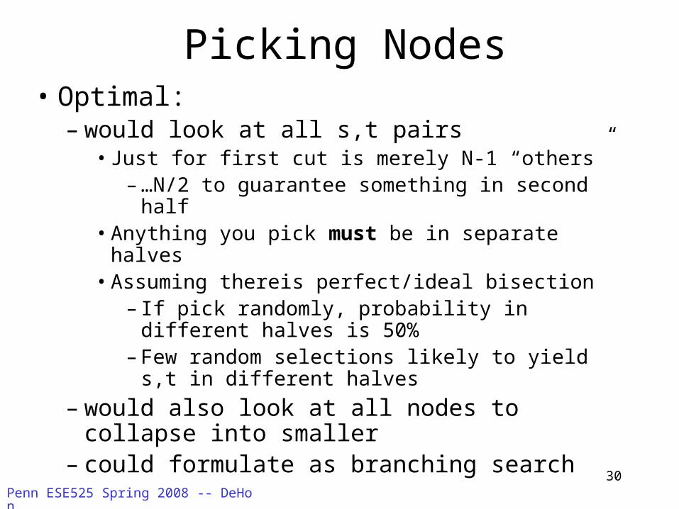
Picking Nodes• Optimal:
– would look at all s,t pairs• Just for first cut is merely N-1 “others”
– …N/2 to guarantee something in second half• Anything you pick must be in separate halves• Assuming thereis perfect/ideal bisection
– If pick randomly, probability in different halves is 50%
– Few random selections likely to yield s,t in different halves
– would also look at all nodes to collapse into smaller
– could formulate as branching search
Penn ESE525 Spring 2008 -- DeHon 31
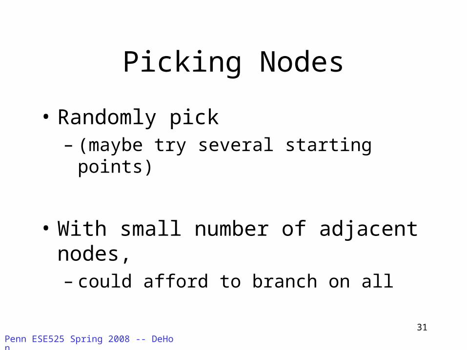
Picking Nodes
• Randomly pick – (maybe try several starting points)
• With small number of adjacent nodes,– could afford to branch on all

Penn ESE525 Spring 2008 -- DeHon 33
Min Cut Replication
• Noted last time could use replication to reduce cut size– Observed could use FM to replicate
• Can solve unbounded replication optimally with mincut
[Liu,Kuo,Cheng TRCAD v14n5p623]

Penn ESE525 Spring 2008 -- DeHon 34
Min-Cut Replication
• Key Idea:– Create two copies of net
• Connect super src/sink to both• reverse links on “to” second copy• Provide directional “free” links between them
– Take mincut • S=reachable from src; T=reachable from sink• R=rest replication set
– Allows nodes to be associated with both ends
Penn ESE525 Spring 2008 -- DeHon 35
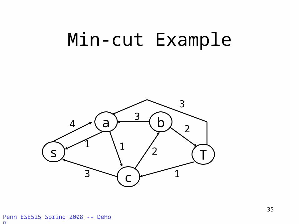
Min-cut Example
s
c
a b
13
1
43
1 2
2
3
T

Penn ESE525 Spring 2008 -- DeHon 36
Min-cut Example
s
c
a b
13
1
43
1 2
2
3
T
s’
c’
a’ b’
13
1
43
1 2
2
3
T’

Penn ESE525 Spring 2008 -- DeHon 37
Min-cut Example
s
c
a b
13
1
43
1 2
2
3
T
s’
c’
a’ b’
13
1
43
1 2
2
3
T’
S* T*

Penn ESE525 Spring 2008 -- DeHon 38
Min-cut Example
s
c
a b
13
1
43
1 2
2
3
T
S’
b’
a’ b’
13
1
43
1 2
2
3
T’
S* T*

Penn ESE525 Spring 2008 -- DeHon 39
Min-cut Example
s
c
a b
13
1
43
1 2
2
3
T
S’
c’
a’ b’
13
1
43
1 2
2
3
T’
S* T*
Start Net flowfind path

Penn ESE525 Spring 2008 -- DeHon 40
Min-cut Example
s
c
a b
13
1
43
1 2
2
3
T
S’
c’
a’ b’
13
1
43
1 2
2
3
T’
S* T*
Cont. net flowfind path

Penn ESE525 Spring 2008 -- DeHon 41
Min-cut Example
s
c
a b
13
1
43
1 2
2
3
T
S’
c’
a’ b’
13
1
43
1 2
2
3
T’
S* T*
How much onthis path?

Penn ESE525 Spring 2008 -- DeHon 42
Min-cut Example
s
c
a b
13
1
43
1 2
2
3
T
S’
c’
a’ b’
13
1
43
1 2
2
3
T’
S* T*
Another path?
3
33
3
3
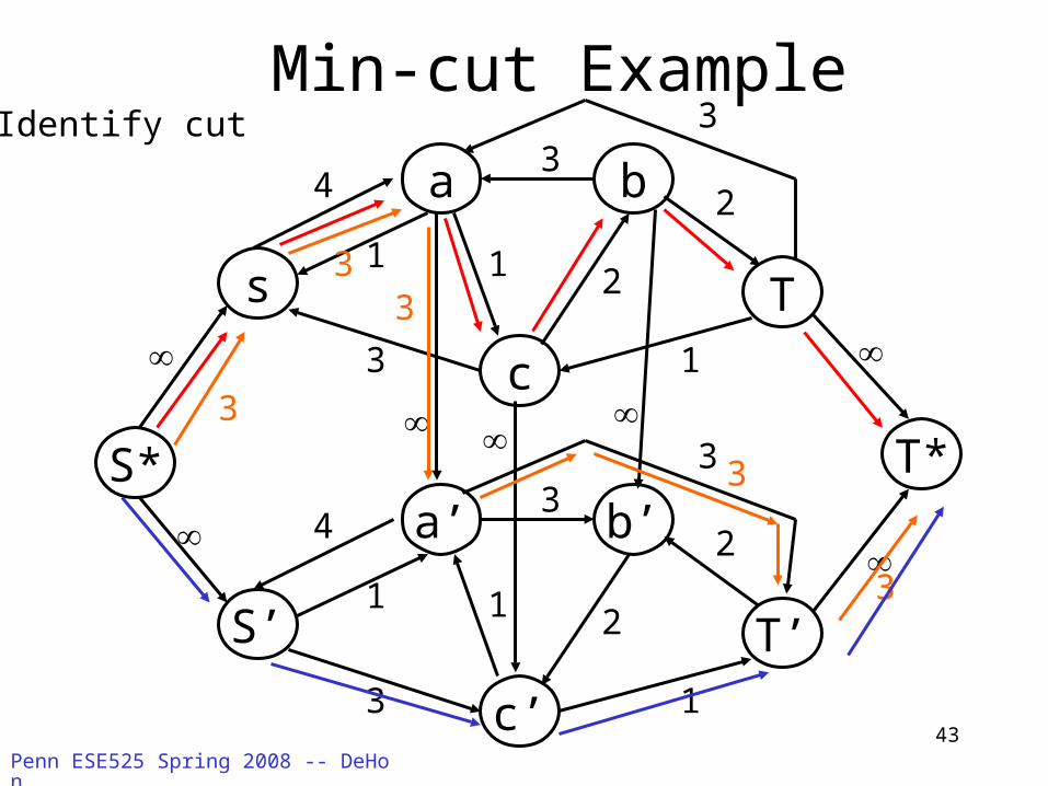
Penn ESE525 Spring 2008 -- DeHon 43
Min-cut Example
s
c
a b
13
1
43
1 2
2
3
T
S’
c’
a’ b’
13
1
43
1 2
2
3
T’
S* T*
Identify cut
3
33
3
3

Penn ESE525 Spring 2008 -- DeHon 44
Min-cut Example
s
c
a b
13
1
43
1 2
2
3
T
S’
c’
a’ b’
13
1
43
1 2
2
3
T’
S* T*
Shows cut
3
33
3
3
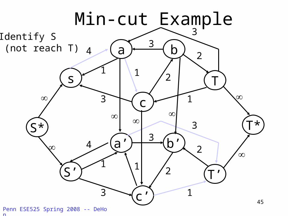
Penn ESE525 Spring 2008 -- DeHon 45
Min-cut Example
s
c
a b
13
1
43
1 2
2
3
T
S’
c’
a’ b’
13
1
43
1 2
2
3
T’
S* T*
Identify S (not reach T)

Penn ESE525 Spring 2008 -- DeHon 46
Min-cut Example
s
c
a b
13
1
43
1 2
2
3
T
S’
c’
a’ b’
13
1
43
1 2
2
3
T’
S* T*
Identify T
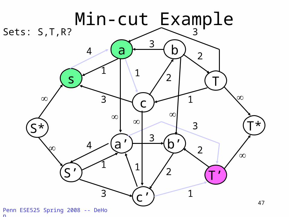
Penn ESE525 Spring 2008 -- DeHon 47
Min-cut Example
s
c
a b
13
1
43
1 2
2
3
T
S’
c’
a’ b’
13
1
43
1 2
2
3
T’
S* T*
Sets: S,T,R?
Penn ESE525 Spring 2008 -- DeHon 48
Min-cut Example
s
c
a b
13
1
43
1 2
2
3
T
S’
c’
a’ b’
13
1
43
1 2
2
3
T’
S* T*
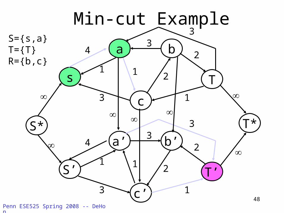
S={s,a}T={T}R={b,c}
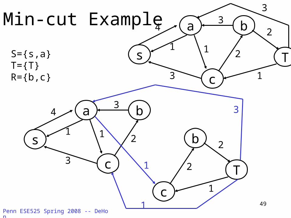
Penn ESE525 Spring 2008 -- DeHon 49
Min-cut Example
S={s,a}T={T}R={b,c}
s
c
a b
3
1
43
1 2
c
b
1
2
2
T
s
c
a b
13
1
43
1 2
2
3
T
1
1
3

Penn ESE525 Spring 2008 -- DeHon 50
Replication Note
• Cut of minimum width is not unique– Similar to phenomenon saw in LUT covering
with network flow
• Want to identify minimum size replication set for given flow
• Can do by reweighing graph and another min-cut– Idea: weight on replication connections
• Minimize cut minimize replication set
– See Mak/Wong TRCAD v16n10p1221

Penn ESE525 Spring 2008 -- DeHon 51
Admin
• Monday reading online
• Homework 3 due Monday

Penn ESE525 Spring 2008 -- DeHon 52
Big Ideas
• Divide-and-Conquer• Techniques
– flow based– numerical/linear-programming based– Transformation constructs
• Exploit problems we can solve optimally– Mincut– Linear ordering