4 May 2007 LIGO-G070283-00-K

Pendulum Modeling in Mathematica™ and Matlab™

IGR Thermal Noise Group Meeting

4 May 2007

4 May 2007 LIGO-G070283-00-K 2

The X-Pendulum

Developed as a low frequency vibration isolator for TAMA

2D version1D version

4 May 2007 LIGO-G070283-00-K

Pendulum Modelling

Wanted an AdvLIGO SUS design model to go beyond the Matlab model of Torrie, Strain et al.

Desired features:» Full 3D with provision for asymmetries» Proper blade model» Wire bending elasticity» Arbitrary damping and consequent thermal noise» Export to other environments such as Matlab/Simulink and E2E.

Mathematica code originally developed for modeling the X-pendulum was available -> reuse and extend.

See http://www.ligo.caltech.edu/~e2e/SUSmodels Manual: T020205-00 (-01 pending)

4 May 2007 LIGO-G070283-00-K

The Toolkit

The toolkit is a Mathematica “package”, PendUtil.nb, for specifying different configurations (e.g., quad, triple etc) in a (relatively) user-friendly way

Supported features:» 6-DOF rigid bodies for masses (no internal modes)

» Springs described by an elasticity tensor and a vector of pre-load forces

» Massless wires (i.e., no violin modes) but detailed elasticity model from beam equation

» Arbitrary frequency-dependent damping on all sources of elasticity

» Symbolic up to the point of minimizing the potential to find the equilibrium position

» Calculates elasticity and mass matrices semi-numerically (symbolic partial derivatives of functions with mostly numeric coefficients)

» Eigenfrequencies and eigenmodes calculated numerically

» Arbitrary frequency dependent damping on each different elastic element

» Transfer functions

» Thermal noise plots

» Export of state-space matrices to Matlab and E2E

4 May 2007 LIGO-G070283-00-K 5

Models

Two major families of models have been defined:» The triple models reflect a generic GEO-style pendulum with 3 masses, 6

blade springs and 10 wires.» The quad models reflect a standard AdvLIGO quad pendulum, with 4

masses, 6 blade springs and 14 wires.

Many toy models» LIGO-I two-wire pendulum» Simple pendulum» Simple pendulum on a blade spring» Etc

Steep learning curve but a major new model can be programmed in a day by an experienced user

5

4 May 2007 LIGO-G070283-00-K 6

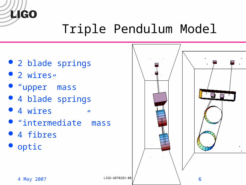
Triple Pendulum Model

2 blade springs 2 wires “upper” mass 4 blade springs 4 wires “intermediate” mass 4 fibres optic

6

4 May 2007 LIGO-G070283-00-K 7

Quad Pendulum

2 blade springs 2 wires “top” mass 2 blade springs 4 wires “upper” mass 2 blade springs 4 wires “intermediate” mass 4 fibres optic

7

4 May 2007 LIGO-G070283-00-K 8

Defining a Model (i)

Define the “variables” (cf. x in the theory - example from the xtra-lite triple):

allvars = {

» x1,y1,z1,yaw1,pitch1,roll1,

» x2,y2,z2,yaw2,pitch2,roll2,

» x3,y3,z3,yaw3,pitch3,roll3

};

Define the “floats” (cf. q in the theory):» allfloats = {

–qul,qur,qlf,qlb,qrf,qrb» };

Define the “parameters” (cf. s in the theory): allparams = {

» x00, y00, z00, yaw00, pitch00, roll00

};

8

4 May 2007 LIGO-G070283-00-K 9

Defining a Model (ii)

Define coordinate lists for rigid bodies of interest: optic = {x3, y3, z3, yaw3, pitch3, roll3};

support = {x00, y00, z00, yaw00, pitch00, roll00};

Define coordinate lists for points on rigid bodies massUl={0,-n1,d0}; (* left wire attachment point on upper mass *)

Define list of gravitational potential terms: gravlist = {}; (* initialize list *)

AppendTo[gravlist, m3 g z3]; (* typical item *)

9

4 May 2007 LIGO-G070283-00-K 10

Defining a Model (iii)

Define list of wires, each with the following format {

» coordinate list defining first mass,

» attachment point for first mass (local coordinates),

» attachment vector for first mass,

» coordinate list defining second mass,

» attachment point for second mass (local coordinates),

» attachment vector for second mass,

» Young's modulus,

» unstretched length,

» longitudinal elasticity,

» vector defining principal axis 1,

» moment of area along principal axis 1,

» moment of area along principal axis 2,

» linear elasticity type,

» angular elasticity type,

» torsional elasticity type,

» shear modulus,

» cross sectional area for torsional calculations,» torsional stiffness geometric factor

}

10

4 May 2007 LIGO-G070283-00-K 11

Defining a Model (iv)

Define list of springs, each with following format: {

» coordinate list defining first mass,

» attachment point for first mass (local coordinates),

» attachment angles for first mass (yaw, pitch, roll),

» coordinate list defining second mass,

» attachment point for second mass (local coordinates),

» attachment angles for second mass (yaw, pitch, roll),

» damping type,

» 6x6 elasticity matrix,

» 1*6 pre-load force/torque vector

}

Define kinetic energy IM3 = {{I3x, 0, 0}, {0, I3y, 0}, {0, 0, I3z}}; (* typical MOI tensor)

kinetic = (

» …

» +(1/2) m3 Plus@@(Dt[b2s[optic,COM],t]^2)

» +(1/2) omegaB[yaw3, pitch3, roll3].IM3.omegaB[yaw3, pitch3, roll3]

» …

);

11

4 May 2007 LIGO-G070283-00-K 12

Defining a Model (v)

Define default values of constants defaultvalues = {

» g -> 9.81, (* value given numerically *)

» …

» m3 -> Pi*r3^2*t3, (* value given in terms of other constants *)

» …

» x00 -> 0, (* value for nominal position of structure *)

» y00 -> 0,

» z00 -> 0,

» …

» damping[imag,dampingtype] -> (phi&) (* value for frequency dependence of damping *)

» …

};

Define starting point for finding equilibrium position: startpos = {

» x1 ->0,

» y1 ->0,

» …

};

12

4 May 2007 LIGO-G070283-00-K 13

Defining a Model (vi)

Define model-specific utilities:» A function to list eigenmodes in a table» pretty[eigenvector]

» A function to plot eigenmode shapes » eigenplot[eigenvector, amplitude, {viewpoint}]

» Vectors representing force and displacement inputs and displacement outputs of interest

» structurerollinput = makeinputvector[roll00];

» opticxinput = makefinputvector[x3];

» opticx = makeoutputvector[x3];

» Rotation matrices to put angle variables in a more easily interpretable basis:

» e2ni;

13

4 May 2007 LIGO-G070283-00-K 14

Sample Output (i)

Transfer function from x displacement of support to x motion of optic (quad model, reference parameters of 20031114):

4 May 2007 LIGO-G070283-00-K 15

Damping

Damping can be represented by a complex elastic modulus:

Strictly, the Kramers-Kronig relation applies:

However often the variation in the real part can be ignored:

Need to consider total potential as sum of terms, each with different damping:

15

k→ k0 ′ε ω( )+ i ′′ε ω( )( )

′ε ω( )−1 =2

πPV

′′ε x( )

x −ω−∞

∞

∫ dx ′′ε ω( ) =−2

πPV

′ε x( ) −1

x −ω−∞

∞

∫ dx

k→ k0 1+ iφ f( )( )

P= Pi∑ ′ε i f( )+ i ′′ε i f( )( )

4 May 2007 LIGO-G070283-00-K 16

Sample Output (ii)

Thermal noise in x motion of optic (quad model, reference parameters of 20031114):

4 May 2007 LIGO-G070283-00-K 17

Export to Matlab/Simulink

17

4 May 2007 LIGO-G070283-00-K 18

Export to E2E

4 May 2007 LIGO-G070283-00-K 19

Application to Quad Controls

Good agreement after adding lots of new physics:» Improved wire flexure

correction» Blade lateral

compliance» Blade geometric

antispring effect» Non-diagonal

moment of inertia tensors

IDpitchxyzyawrollxypitchyawxyzyawpitchrollyawpitch?rollxzrollzroll

f (theory)0.3950.4430.4640.5950.6850.8100.9871.0431.1671.4281.9812.0952.3622.5382.8182.7623.1673.2283.3323.4013.7935.120

17.70025.741

f (exp)0.4030.4400.4640.5490.6840.7940.9891.0381.3551.4281.9782.0752.2222.5152.5762.7343.1493.1623.3333.3813.5895.029

??

4 May 2007 LIGO-G070283-00-K 20

Dissipation Dilution

Often said: main restoring force in a pendulum is gravitational therefore no loss -> “dissipation dilution”

Not true! Gravitational force is purely vertical. Actual restoring force is sideways component of tension in

wire Gravity’s only contribution is to tension the wire. Other forms of tension are equivalent (cf. violin modes also

low-loss What is it about tension?

20

4 May 2007 LIGO-G070283-00-K 21

Mass on spring Force: Frequency: Amplitude (phasor): Velocity (phasor): Force (phasor): Power (average): Energy (max): Decay time (energy): Decay time (amp.)

Non-dilution case (vertical)

21

F =−k l −l0( )

F =−ALk0 1+ iφ( )

P =Fv=AL2k0φω

E =12 k0AL

2

AL

v=iωAL

2

φω1

φω

ω =k

m

4 May 2007 LIGO-G070283-00-K 22

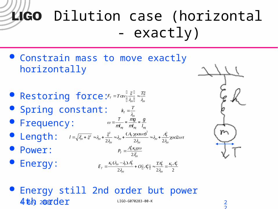
Dilution case (horizontal - exactly)

Constrain mass to move exactly horizontally

Restoring force: Spring constant: Frequency: Length: Power: Energy:

Energy still 2nd order but power 4th order

FT =T sinxleq

⎛

⎝⎜

⎞

⎠⎟ ≈

Txleq

kT =Tleq

ω =T

mleq=mg

mleq=g

leq

l = leq2 + x2 ≈leq +

x2

2leq≈leq +

AT cosωt( )2

2leq≈leq +

AT2

2leqcos2ωt

PT =AT

4k0φω2leq

2

ET =k0 leq −l0( )AT

2

2leq+O AT

4⎡⎣ ⎤⎦≈TAT

2

2leq=

kT AT2

2

4 May 2007 LIGO-G070283-00-K 23

But what about pendulums?!

In a pendulum, mass really moves on an arc. Doesn’t matter! Normal mode analysis can’t tell the difference! Eigenmodes are always linear in coordinates used. Analyze in r,theta -> eigenmode is arc Analyze in x, z -> eigenmode is straight line Same frequencies!

4 May 2007 LIGO-G070283-00-K 24

What about pendulums (ii)

24

Two independent reasons why pendulums have low loss.» Restoring force is sideways component of tension» Energy may then be off-loaded into gravitational potential -> stretch of spring

less even than second order

Depends on bounce and pendulum mode frequencies» Usual case, bounce frequency high -> mass moves on arc.» Very low bounce frequencies (superspring) -> mass really does move

horizontally

4 May 2007 LIGO-G070283-00-K 25

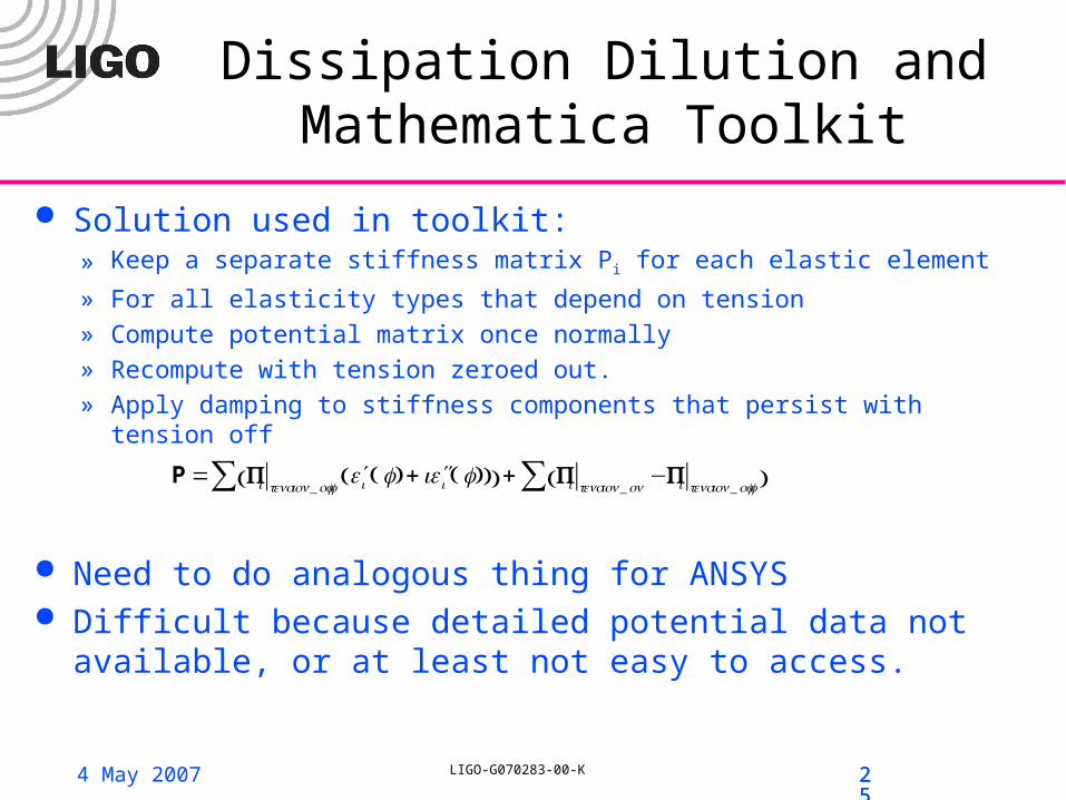
Dissipation Dilution and Mathematica Toolkit

Solution used in toolkit: » Keep a separate stiffness matrix Pi for each elastic element

» For all elasticity types that depend on tension» Compute potential matrix once normally» Recompute with tension zeroed out.» Apply damping to stiffness components that persist with tension off

Need to do analogous thing for ANSYS Difficult because detailed potential data not available, or at

least not easy to access.

25

P= Pi tension_off′ε i f( )+ i ′′ε i f( )( )( )∑ + Pi tension_on

−Pi tension_off( )∑

4 May 2007 LIGO-G070283-00-K 26

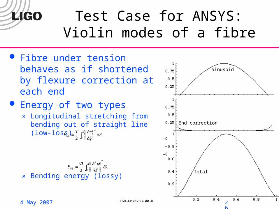
Test Case for ANSYS: Violin modes of a fibre

Fibre under tension behaves as if shortened by flexure correction at each end

Energy of two types» Longitudinal stretching from bending out

of straight line (low-loss)

» Bending energy (lossy)

EVB =YI2

d2ydl2

⎛

⎝⎜⎞

⎠⎟0

L

∫2

dl

EVL =T2

dydx

⎛⎝⎜

⎞⎠⎟

2

dx0

L

∫

Sinusoid

End correction

Total

4 May 2007 LIGO-G070283-00-K 27

Fibre results

Fused silica, 350 mm long, 0.45 mm diameter

Integrand of the two types

» Longitudinal ->» Total 17.3 mJ for 10 mm amplitude

» Bending ->» Total 0.256 mJ for 10 mm amplitude

Dissipation dilution factor 67.6 Will compare to ANSYS