License and Terms: This document is copyright 2021 the Author(s); licensee Beilstein-Institut.

This is an open access work under the terms of the Creative Commons Attribution License (https://creativecommons.org/licenses/by/4.0). Please note that the reuse,redistribution and reproduction in particular requires that the author(s) and source are credited and that individual graphics may be subject to special legal provisions.

The license is subject to the Beilstein Archives terms and conditions: https://www.beilstein-archives.org/xiv/terms.The definitive version of this work can be found at https://doi.org/10.3762/bxiv.2021.22.v1

This open access document is posted as a preprint in the Beilstein Archives at https://doi.org/10.3762/bxiv.2021.22.v1 and isconsidered to be an early communication for feedback before peer review. Before citing this document, please check if a final,peer-reviewed version has been published.

This document is not formatted, has not undergone copyediting or typesetting, and may contain errors, unsubstantiated scientificclaims or preliminary data.

Preprint Title Development of QSAR ensemble models for predicting the PAMPAEffective Permeability of new, non-peptidic leads with potentialantiviral activity against the coronavirus SARS-CoV-2.

Authors Chrysoula Gousiadou, Philip Doganis and Haralambos Sarimveis

Publication Date 15 März 2021

Article Type Full Research Paper

Supporting Information File 1 Supporting Information.xlsx; 1.2 MB

ORCID® iDs Chrysoula Gousiadou - https://orcid.org/0000-0002-7093-3055

1

Development of QSAR ensemble models for predicting the PAMPA Effective

Permeability of new, non-peptidic leads with potential antiviral activity against the

coronavirus SARS-CoV-2.

C. Gousiadoua , P. Doganisa, H. Sarimveisa

a. School of Chemical Engineering, National Technical University of Athens, Heroon

Polytechneiou 9, 15780, Zografou, Athens, Greece

Corresponding Author:

Chrysoula Gousiadou, Tel: +45 91942533, email: cgousiadou@gmail.com

Abstract

From the onset of the pandemic caused by the virus SARS-CoV-2, the scientific community

responded– with a sense of urgency – by intensifying efforts to provide drugs effective against

the disease COVID-19. To strengthen this efforts, a consortium of researchers initiated in

March 2020 the “COVID Moonshot project” that has been accepting public suggestions for

computationally triaged, synthesized, and tested molecules, with experimental data made

publicly available. The main goal of the project was to identify through Fragment Based Drug

Design (FBDD) small molecules with activity against the virus, for oral treatment. Since orally

administered drugs are introduced to the bloodstream through absorption via the small intestine

pathway, the ability of a drug to readily cross the intestinal cell membranes and enter circulation

is decisively influencing its bioavailability. This explains the need to evaluate and optimize a

drug’s membrane permeability in the early stages of drug discovery to avoid failures in late-

stage drug development owing to incomplete absorption and poor bioavailability. In our present

2

work, as a contribution to the ongoing scientific efforts, we have employed advanced Machine

Learning techniques, including stacked model ensembles, to develop QSAR tools for modelling

the PAMPA Effective Permeability (passive diffusion) of orally administered drugs. By

applying feature elimination methods, we identified a set of 61 features (descriptors) most

relevant in explaining drug cell permeability and used these features to develop the models. The

QSAR models were subsequently used to predict the PAMPA Effective Permeability of

molecules included in datasets made available through the COVID Moonshot project. Our

models were shown to be robust and may provide a promising framework for predicting the

potential permeability of molecules not yet synthesized, thus guiding the process of drug design.

Keywords: covid-19; PAMPA; permeability; QSAR; ensemble modelling; descriptors

Introduction

Faced with unprecedented challenges against public health in the outbreak of the pandemic,

medical scientists swiftly responded by initially adopting drug repositioning approaches, i.e.,

screening already approved drugs - or candidates in advanced clinical research – for their

efficacy to inhibit the course of the disease COVID-19 for immediate use [1, 2]. Such

approaches proved highly effective in the past, as in cases like zidovudine (AZT) [3] and

sildenafil (Viagra) [4], which, although being initially developed for cancer (zidovudine) and

coronary disease (sildenafil) treatment, were successfully repurposed for the therapy of

HIV/AIDS and erectile dysfunction, respectively. On these grounds, drugs with broad chemical

diversity and therapeutic use were investigated in more than 5000 clinical studies [1, 5-8]. The

findings revealed that dexamethasone - an anti-inflammatory corticosteroid used since the

1960s – decreased the mortality rate among patients on ventilators, whilst remdesivir, an

antiviral drug originally developed to treat hepatitis C and subsequently used during the Ebola

3

outbreak, accelerated recovery for hospitalized patients with severe COVID-19 and became the

first drug to receive emergency use authorization from the U.S. Food and Drug Administration

(FDA) for COVID-19 treatment [9, 10].

As new information on the nature and special characteristics of the virus became available,

efforts for new, target-specific drugs were intensified. SARS-CoV-2 enters human cells and co-

opts ribosomes to translate its viral RNA into two polyproteins. These polyproteins are in turn

cleaved into individual peptides by an enzyme called the main protease, or Mpro . Because of its

early, essential role in the viral replication cycle, Mpro is a target for drug discovery [11].

Previous knowledge on the related coronavirus MERS-CoV allowed researchers to identify

potent peptidomimetic inhibitors of Mpro, but their peptidic nature complicated oral delivery

[11]. Aiming to design target-specific drugs for oral use, an international team led by Martin

Walsh and Frank von Delft from Diamond Light Source - the United Kingdom’s national

synchrotron facility - and Nir London from the Weizmann Institute in Israel used Fragment

Based Drug Design (FBDD) to identify a set of chemical fragments that attach to the protein

[11]. Soon after, on 17 March 2020, in collaboration with Diamond, the machine-learning

company PostEra led by its co-founder and chief scientific officer Alpha Lee, joined the effort

by offering to connect the dots from fragments to viable drugs against COVID-19 [12]. PostEra

uses AI algorithms to map routes for drug synthesis to speed the drug-discovery process, but to

do so, some design ideas would be needed. So, Lee launched the COVID Moonshot project on

the internet, to crowdsource drug designs from medicinal chemists. To date, over 16.000 unique

molecular designs from contributors around the world have flooded into the submission’s site

set up for the effort [12].

FBDD is a powerful method, used to develop potent small-molecule compounds starting from

fragments binding weakly to protein targets. Rather than starting from a substrate-based

molecule like the peptidomimetics, or screening hundreds of thousands of drug-sized

4

molecules, FBDD starts with more limited libraries of smaller molecules, or fragments. Because

there are fewer possible small fragments than drug-sized molecules, FBDD can survey chemical

space more comprehensively to find the most attractive starting points for medicinal chemistry.

Also, because fragments are so small, they tend to bind to more sites on proteins, which

facilitates lead identification [12, 13]. A subsequent merging or linking of fragments to produce

a larger, more potent molecule is often a next step in the process of drug discovery.

Whilst the bioactivity of fragments designed and submitted to the project is currently under

investigation and while sub-micromolar IC50 has been reported for a number of them [11, 12],

important factors like permeability, selectivity, pharmacokinetics, pharmacodynamics and

toxicity remain to be optimized to improve their drug-like profile.

In pharmacokinetics and pharmacology, ADME is an abbreviation for "absorption, distribution,

metabolism & excretion", used to describe the disposition of a pharmaceutical compound within

an organism. These four criteria determine the drug levels and kinetics of drug exposure to the

tissues and consequently influence the performance and pharmacological activity of a

compound as a drug [14]. For the orally administered drugs in particular, introduced via the

intestinal pathway to the bloodstream, a high degree of absorption results in high

bioavailability. A key factor decisively influencing and regulating a drug’s absorption is the

drug’s permeability across the biological membranes. Indeed, before a drug can reach the

systemic circulation it needs to cross several semipermeable cell membranes, which explains

the need to evaluate and optimize a drug’s permeability in the early stages of drug discovery to

avoid failures in late-stage development owing to incomplete absorption and poor

bioavailability and reduce attrition rate [14].

Drugs cross cell membranes by passive diffusion, facilitated passive diffusion, active transport,

and pinocytosis [15]. The small intestine is the main site of absorption via passive diffusion for

the majority of orally administered drugs. During this process, drugs diffuse across a cell

5

membrane from a region of high concentration (e.g., gastrointestinal fluids) to one of low

concentration (e.g., blood). The diffusion rate is affected by the drug’s lipid solubility, size,

degree of ionization, and the area of absorptive surface. Because the cell membrane is lipoid,

lipid-soluble drugs diffuse most rapidly. Also, small molecules tend to penetrate membranes

more rapidly than larger ones [15].

The need for a quick and early estimate of drug permeability resulted in the development of

various methods to be used for high-throughput screening of drug candidates. Indeed, the fact

that intestinal drug transport is strongly connected to several physicochemical properties is

described by Lipinski's “rule of five”, which indicates whether a drug is likely to be absorbed

after oral administration [16, 17]. This fairly simple computational approach is based on the

concept that five physicochemical properties of drugs, i.e., molecular weight, lipophilicity,

polar surface area, hydrogen bonding and charge affect the interaction between the drugs and

the membranes, having significant impact on their permeability, especially via passive

diffusion.

Further in vitro methods to predict in vivo absorption - though not exclusively via passive

diffusion - include tissue-based permeation models that closely mimic the in vivo situation from

an anatomical, biochemical and structural point of view as well as cell-based systems like the

well-known human colorectal adenocarcinoma (Caco-2) cell line and the Madin Darby canine

kidney (MDCK) cell line. The widely used Caco-2 cell line generates reproducible permeability

results on a high-throughput basis. Notwithstanding their popularity and reasonable predictive

power, cell-based permeation systems suffer from several shortcomings, including a relative

incompatibility with food components and certain pharmaceutical excipients, the absence of

CYP3A4 and the lack of a mucus layer. In addition, they are time-consuming and require

expensive preparation steps [18].

6

As a result of the increased demand for rapid, cell-free permeation systems, Kansy et al. [19]

first introduced the Parallel Artificial Membrane Permeability Assay (PAMPA), which is an in

vitro method used to measure permeability only by passive diffusion and has since been adopted

as the primary permeability screening to assess the passive diffusion of compounds in practical

applications [20]. The PAMPA system is a ‘sandwich’ consisting of two 96-well plates and

includes three compartments. The method measures the permeability of substances moving

from a donor compartment, through a lipid-infused artificial membrane into an acceptor

compartment [19, 20]. The donor, membrane and acceptor compartments emulate the

gastrointestinal tract, the intestinal epithelium and the blood circulation, respectively. The

original PAMPA membrane was formed using lecithin solution in dodecane. To date, PAMPA

models have been developed that exhibit a high degree of correlation with permeation across a

variety of barriers, including Caco-2 cultures [21, 22], the gastrointestinal tract [23], blood–

brain barrier[24] and skin [25]. The simplicity and stability of the PAMPA system allows for

variability in the experimental settings, e.g., changing the pH values in the donor compartment

offers the possibility to measure permeability under different physiological conditions in the

intestinal pathway [18, 19]. PAMPA measurements are shown to compare well with human

intestinal absorption, except for some problematic cases concerning compounds with limited

solubility or specific drug classes and compounds absorbed by active transport [26].

As well as using experimental studies, the possibility of employing computational approaches

- like quantitative structure-activity relationship (QSAR) models - to predict drug permeability

in the early stages of drug discovery is attractive both from a financial and time-saving

perspective. Through virtual screening, in silico approaches may provide insights to the

potential permeability of molecules not yet synthesized, thus guiding the process of drug design.

Nevertheless, as every QSAR model can only be as good as the quality of data used to create

it, special consideration should be given to the consistency, quality and completeness of the

7

permeability data used in the analyses. Permeability measurements heavily depend on the

applied experimental protocols and differences in factors like the assay pH, system temperature,

content of membrane [23, 27, 20] etc. result in varying experimental permeability values.

Hence, in principle, homogenous datasets - created with the same experimental protocol - are

preferably used to build reliable QSAR permeability models.

In the present work, as a contribution to the COVID Moonshot project, we employed advanced

Machine Learning algorithms to create sophisticated “stacked regression” ensemble QSAR

models for predicting drug permeability. By ensembling diverse sets of learners together we

created second level “metalearners” with enhanced predictive performance. To build the

models, we used a publicly available dataset [20, 28-31] (Supporting Information, sheet S1.1)

with recorded permeability values for 190 molecules, measured using the same experimental

protocol [28-31]. As different types of measurements result to different PAMPA permeability

coefficients [20, 27], we note that in the present work we have modelled the Effective

Permeability Coefficient (logPe), analytically described in the “Methods” section.

Our QSAR models were robust and well validated through external validation and may provide

a promising framework for anticipating drug PAMPA permeability. We subsequently used the

QSAR models to predict the membrane permeability of 4520 molecules, contributed by

medicinal chemists to the COVID Moonshot Project and downloaded from the PostEra site [12]

on 01-MAY-2020, as well as 1561 molecules downloaded from the same site on 02

FEBRUARY 2021 for which biological activity has been recorded. Our goal in doing so, was

to join and strengthen the ongoing research efforts towards the development from scratch of

new target-specific drugs for COVID-19 treatment. Arguably, although mass vaccination with

highly effective vaccines available today will safeguard public health, it cannot not be

considered a panacea. Vaccines for a disease do not always guarantee its eradication [32] and

high rates of mutations in the genome of the virus may reduce their effectiveness. Additionally,

8

a major drawback in acquiring mass immunity through vaccination can be the reluctance of

large parts of a population to get vaccinated, giving birth to strong anti-vaccine movements. On

these grounds, target-specific drugs with statistically significant effects on the course of the

disease will make a real difference for COVID-19 patient survival and build confidence that

there is a cure for COVID-19.

Results and discussion

Data Preprocessing and Feature Selection

An initial exploratory analysis of the dataset (190 molecules, 232 descriptors) revealed a high

correlation (>0.80) between 127 descriptors. As it is always desirable to have a reduced set of

uncorrelated, nonredundant, and informative descriptors that allow for interpretable prediction

models, we reduced data dimensionality using feature elimination methods. Feature selection

was performed using the training set of 141 molecules with 232 descriptors and the

corresponding logPe values. The method selected for the feature elimination was based on a

wrapper approach [33]. Wrapper methods are search algorithms that treat the predictors as

inputs and utilize model performance as the criterion to be optimized [34]. Using the caret

package in R (caret package - version 6.0-84) we performed a simple backwards selection of

descriptors (Recursive Feature Elimination, RFE) with Random Forest (randomForest package

- version 4.6-14) [35]. Random Forest has a built-in feature selection [36] as well as variable

importance estimation utilised for the RFE approach [35, 37]. We used the version of the

algorithm that incorporates resampling (rfe) [37] and applied an outer resampling method of

20-fold cross-validation with three repeats to reduce the risk of overfitting of the model to the

descriptors and to get performance estimates that incorporate the variation due to feature

selection. By employing the resampling method, we improved the generalization performance

of the model and obtained a more probabilistic assessment of descriptor importance than a

ranking based on a single fixed data set. The best performance was based on the Root-Mean

9

Square-Error (RMSECV) [38] and corresponded to a subset of 61 descriptor variables - ranked

according to their significance in predicting the logPe values (Figure 1), (Supporting

Information S1.5) - which we further used to build our models.

Figure 1. Selection of Descriptors. Feature selection with Random

Forest (Recursive Feature Elimination) for the effective permeability

(logPe) modelling, using the 141 molecules included in the train set.

The best performance based on the Root-Mean Square-Error

(RMSEcv) [38] corresponded to a subset of 61 descriptor variables

selected as most significant in predicting the logPe values.

For modelling the effective membrane permeability coefficient (logPe), the 61 selected features

were further scaled and centered based on the combined - prior to partitioning into training and

test sets - model development and initial evaluation data (174 molecules, Supporting

information, sheet S1.3). Subsequently, we used the training data (Supporting Information,

sheet S1.3a) and employed a sophisticated ensemble modelling approach known as “stacked

regression” [39]. Ensemble approaches combine the predictions of multiple learning

algorithms for obtaining improved predictive performance, which could not otherwise be

obtained from any of the constituent learners alone. It is somehow the equivalent of seeking the

“wisdom of the crowd” in making decisions. Nevertheless, although an ensemble has multiple

base models within the model, it acts and performs as a single model [40]. The advantage in

creating such a “metalearner” is that the generalization error of the prediction is minimized by

deducing the biases of the base models with respect to a provided learning set. This deduction

10

proceeds by generalizing in a second space - whose inputs are the predictions of the base

learners on a given dataset and whose output is the actual outcome - and trying to make

predictions on new, unseen data [41]. Indeed, better generalisation performance from ensemble

modelling arising from a more diverse ensemble of base models underpins Breiman’s original

justification for Random Forest [42].

In the present study, models suitable to be combined in an ensemble were generated by using

the selected 61 descriptors to build a series of learners - on the training set of 141 molecules

(Supporting Information, sheet S1.3a) - and compare their performance. To this end, we used

the caret package to train Machine Learning algorithms of diverse learning styles to choose

those that modelled our data best (Table 1A). Τhe previously performed selection of features

greatly benefited the traditional statistical methods k-nearest neighbors (kNN) and linear

regression (lm), since without a sophisticated variable selection filter they cannot be used

reliably [35]. Feature selection also optimized further the performance of the Random Forest

(rf) algorithm upon retraining [36]. For this exploratory analysis, the algorithms were applied

using their default parameters and a resampling method of 20-fold cross validation with 3

repeats was employed. The resulting Root Mean Square Error and Rsquared values (RMSECV

and ‡R2CV) - calculated according to equations (3) & (2), respectively, and presented as the

average across all folds and repeats of cross-validation - provided an approximate estimate of

the models’ ability to predict unseen data. References for the different Machine Learning

algorithms are given in Table 1A, referred to via their short-hand descriptions for brevity.

Table 1A

Evaluation Metrics of algorithms used for modelling the logPe of 141 molecules in the

train set after feature selection by Recursive Feature Elimination. The results were

obtained via 20-fold cross-validation with 3 repeats. These cross-validation results were

prior to optimizing the algorithms’ hyperparameters.

Root-Mean-Square-Error

(RMSECV)

‡R2CV

Models Min. Mean Max. Min. Mean Max.

rf 0.291 0.667 1.181 0.114 0.670 0.965

xgbTree 0.262 0.653 1.113 0.017 0.665 0.960

11

xgbLinear 0.250 0.687 1.345 0.020 0.628 0.975

knn 0.240 0.708 1.503 0.001 0.614 0.990

lm 0.324 0.851 1.405 0.001 0.586 0.952

glmnet 0.145 0.672 1.094 0.089 0.684 0.990

svmRadial 0.225 0.679 1.215 0.095 0.658 0.965

Algorithms:

rf: Random Forest [35], knn: K-Nearest Neighbor [43], lm: Linear Regression [44], glmnet:

Generalized Linear Regression [45], svmRadial: Support Vector Machines with Radial

Function [46], xgb: eXtreme Gradient Boosting [47]

Table 1B

Inter-model prediction correlation: Pairwise comparison of the cross-validation

results for the selected and optimized models RF1, XGB and KNN, combined in

ensemble models (Table 2). The Metric used is Root Mean Squared Error (RMSECV).

Models RF1 XGB KNN

RF1 1.00 0.85 0.92

XGB 0.85 1.00 0.76

KNN 0.92 0.76 1.00

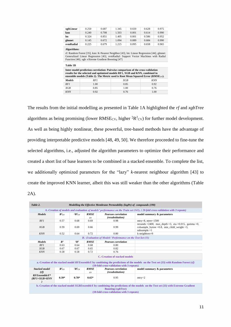
The results from the initial modelling as presented in Table 1A highlighted the rf and xgbTree

algorithms as being promising (lower RMSECV, higher ‡R2CV) for further model development.

As well as being highly nonlinear, these powerful, tree-based methods have the advantage of

providing interpretable predictive models [48, 49, 50]. We therefore proceeded to fine-tune the

selected algorithms, i.e., adjusted the algorithm parameters to optimize their performance and

created a short list of base learners to be combined in a stacked ensemble. To complete the list,

we additionally optimized parameters for the “lazy” k-nearest neighbour algorithm [43] to

create the improved KNN learner, albeit this was still weaker than the other algorithms (Table

2A).

Table 2. Modelling the Effective Membrane Permeability (logPe) of compounds (190)

A.-Creation of models and evaluation of models’ performance on the Train set (141), ( 20-fold cross-validation with 3 repeats)

Models R2CV ‡R2

CV RMSE

CV

Pearson correlation

(resubstitution)

model summary & parameters

RF1 0.57 0.68 0.69 0.98 mtry=8, ntree=1500

XGB 0.59 0.69 0.66 0.99

nrounds =2400, max_depth =3, eta =0.015, gamma =0,

colsample_bytree =0.8, min_child_weight =3,

subsample =1

KNN 0.52 0.64 0.72 0.80 k-neighbors=9

B.- Evaluation of Models’ Performance on the Test Set (33)

Models R2 ‡R2 RMSE Pearson correlation

RF1 0.63 0.64 0.68 0.80

XGB 0.67 0.67 0.65 0.82

KNN 0.58 0.58 0.72 0.76

C.-Creation of stacked models

a.-Creation of the stacked model RFEnsembleX by combining the predictions of the models on the Test set (33) with Random Forest (rf)

(10-fold cross-validation with 3 repeats)

Stacked model

(rf)

R2CV ‡R2

CV RMSE

CV

Pearson correlation

(resubstitution)

model summary & parameters

RFEnsembleX*

(RF1+XGB+KNN

)

0.39* 0.78* 0.65* 0.95 mtry=2

b.-Creation of the stacked model XGBEnsembleX by combining the predictions of the models on the Test set (33) with Extreme Gradient

Boosting (xgbTree)

(10-fold cross-validation with 3 repeats)

12

Stacked model

(xgbTree) R2CV ‡R2

CV RMSE

CV

Pearson correlation

(resubstitution) model summary & parameters

XGBEnsembleX*

*

(RF1+XGB+KNN

)

0.49** 0.77** 0.62** 0.89

nrounds =300, max_depth =2, eta =0.025, gamma =1,

colsample_bytree =0.4, min_child_weight =3,

subsample =0.5

c.-Creation of the stacked model XGBEnsembleX1 by combining the predictions of the models on the Test set (33) with Extreme Gradient

Boosting (xgbTree)

(10-fold cross-validation with 3 repeats)

Stacked model

(xgbTree) R2CV ‡R2

CV RMSE

CV

Pearson correlation

(resubstitution) model summary & parameters

XGBEnsembleX1

***

(RF1+XGB+KNN

)

0.38*** 0.74*** 0.67**

*

0.94

nrounds =50, max_depth =1, eta =0.3, gamma =0,

colsample_bytree =0.6, min_child_weight =1,

subsample =0.75

D.-Evaluation of the stacked Models’ Performance on the Train Set (141)

Models R2 ‡R2 RMSE Pearson correlation

RFEnsembleX 0.86 0.87 0.42 0.94

XGBEnsembleX 0.88 0.91 0.39 0.96

XGBEnsembleX1 0.79 0.81 0.52 0.90

E.-Evaluation of Models’ Performance on the External Validation set (16)

Models R2 ‡R2 RMSE Pearson correlation

RF1 0.59 0.63 0.70 0.80

XGB 0.59 0.59 0.71 0.77

KNN 0.60 0.62 0.70 0.79

RFEnsembleX 0.71 0.72 0.59 0.85

XGBEnsembleX 0.69 0.71 0.61 0.84

XGBEnsembleX1 0.71 0.75 0.60 0.86

The reason for doing so is that in stacked ensemble modelling, the addition of weak algorithms

with diverse learning styles is expected to boost the predictive performance of the ensemble

[39-41]. This assumes that the models have captured different aspects of the data, i.e., their

predictions are not redundant, as is demonstrated for the models combined here (Table 1B,

Figure 3). A visual comparison of the modeling results – based on the evaluation metrics ‡R2CV,

RMSECV and MAEcv [51] - for the prediction performance of the models RF1, XGB and KNN

obtained via cross-validation on the training set (141 molecules) with optimized

hyperparameters is depicted in Figure 2. The Variable Importance rankings obtained with the

different Machine Learning algorithms employed to build the base models RF1, XGB & KNN

are available in Supporting Information S1, sheet S1.5.

13

The fitted models RF1, XGB & KNN were further used to predict the logPe values of the 33

molecules in the test set (Table 2B), which provided a less biased evaluation of the models’

effectiveness in predicting unseen data. We subsequently trained stacked ensembles using

different algorithms (xgbTree with two sets of parameters and rf) and applying 10-fold cross-

validation with 3 repeats, using as input variables the predictions of the base models on the test

set and as output (target) variable the corresponding experimental values of logPe.

The whole process resulted in the creation of the ensemble models RFEnsembleX,

XGBEnsembleX & XGBEnsembleX1 with boosted predictive performance. Since the ensemble

models were built on the combined predictions of the base models on the test set (33 molecules),

we needed first to confirm that they could indeed perform well on the training dataset. We

therefore used the ensembles to predict the logPe values in the train set (141 molecules) and

the results are reported in Table 2D. Subsequently, we evaluated the ability of both the base

Figure 2. Visual comparison of the modeling

results: Evaluation Metrics (‡R2CV, RMSECV and

MAEcv) for the prediction performance of the

models RF1, XGB and KNN obtained via cross-

validation on the training set (141 molecules) with

optimized hyperparameters (Table 2). The

arithmetic mean (circles) and confidence intervals

(95%) are plotted for each distribution. Here,

“Rsquared” refers to ‡R2CV, calculated according to

equation (2) as described above in the “Model

Performance Statistics” section. The Mean

Absolute Error (MAE) [51] evaluation metric, also

presented here, is less sensitive to outliers than

RMSECV.

Figure 3. Pairwise comparison of the cross-validation results

for the models RF1, XGB and KNN (Table 1B). The scatterplot

matrix shows whether the predictions from the models are

correlated. The plotted results, for which correlations are

examined, are based on the Root Mean Squared Error

(RMSECV). If any two models are 100% correlated they are

perfectly aligned around the diagonal. This is best observed

between RF1 and KNN (0.92). The opposite is observed

between KNN and XGB, where the correlation is the lowest

(0.76), meaning that there is limited redundancy in the

information given by these models. This proved valuable for the

creation of the ensemble models RFEnsembleX,

XGBEnsembleX and XGBEnsembleX1 (Table 2).

14

models and the ensembles to make accurate predictions on the hitherto unseen data of the

external validation set, after scaling and centering the descriptors with the same parameters

used for data pre-processing in the combined train-test set. These predictions were completely

unbiased, since the external validation set of 16 molecules had not in any way participated

previously in the development or selection of the models. The ensemble models showed

enhanced performance, making predictions with around 85% correlation to the observed values

(Table 2E, Figure 5), (Supporting Information S1.1).

Figure 4. Gain Curve plots of the log Pe values predicted by the Ensemble Models against the experimental logPe

values. The Gain Curves show whether the models’ predictions are sorted in the same order as the actual log Pe values.

As sorting is the process of placing elements from a collection in some kind of order, the Gain Curve plot depicts how

well the models sort their predictions compared to the true outcome values. For the evaluation of a models’ performance,

the relative Gini score metric is used as follows: relative Gini score equals 1 when a model sorts exactly in the same

order as the actual outcome, whereas the score is close to zero, or even negative when a model sorts poorly compared to

the actual values. The metric therefore can be considered as a measure of how far from “perfect” a model is. The ensemble

models RFEnsembleX, XGBEnsembleX & XGBEnsembleX1 are shown to perform well, with relative Gini scores 0.74,

0.75 & 0.74, respectively [52].

15

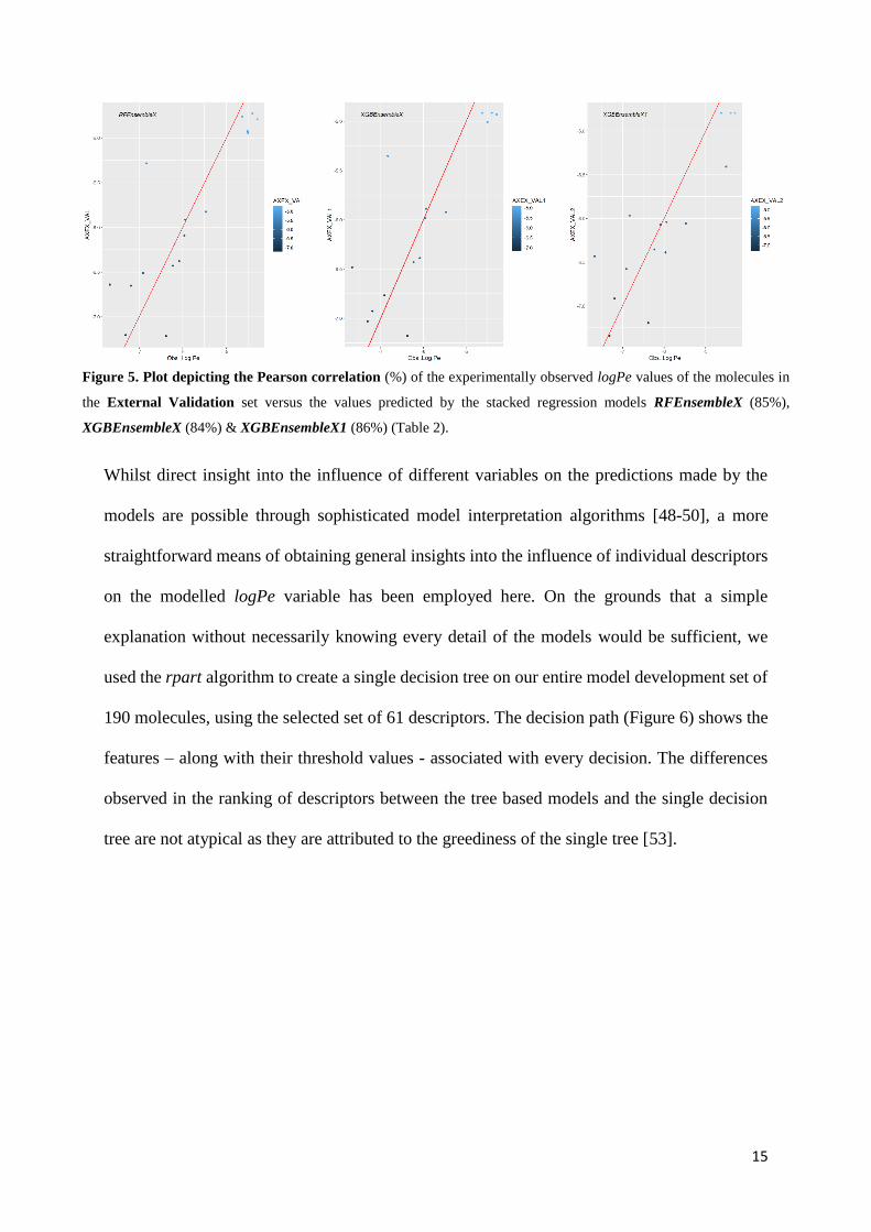
Figure 5. Plot depicting the Pearson correlation (%) of the experimentally observed logPe values of the molecules in

the External Validation set versus the values predicted by the stacked regression models RFEnsembleX (85%),

XGBEnsembleX (84%) & XGBEnsembleX1 (86%) (Table 2).

Whilst direct insight into the influence of different variables on the predictions made by the

models are possible through sophisticated model interpretation algorithms [48-50], a more

straightforward means of obtaining general insights into the influence of individual descriptors

on the modelled logPe variable has been employed here. On the grounds that a simple

explanation without necessarily knowing every detail of the models would be sufficient, we

used the rpart algorithm to create a single decision tree on our entire model development set of

190 molecules, using the selected set of 61 descriptors. The decision path (Figure 6) shows the

features – along with their threshold values - associated with every decision. The differences

observed in the ranking of descriptors between the tree based models and the single decision

tree are not atypical as they are attributed to the greediness of the single tree [53].

16

Figure 6. Single decision tree created on the whole dataset (190 molecules) using the 61 descriptors selected

by Recursive Feature Elimination (RFE) with Random Forest. The decision path clarifies which features are

associated with every decision as well as the threshold values of the top descriptors that are responsible for a

molecule having high/low effective permeability (logPe) at pH 7.4. The results are presented in mean values of

logPe, along with the number and percentage of molecules corresponding to these values. The logPe values of

the 190 molecules are depicted progressively from white (low permeability) to deep blue (high permeability).

According to the rough classification scheme introduced in the section “Permeability Measurements &

Experimental Setup” where the cut-off logPe value is -6.2 [20], the tree classifies 94 molecules as having

“higher permeability” (logPe ≥ -6.2) and 96 as having “lower permeability” (logPe < -6.2), whilst 92 and 98

molecules are experimentally shown to have high/ low permeability, respectively, according to the PAMPA

assay results.

Discussion

Across all three methods (rf, xgboost, knn) used to create the QSAR models for modelling

logPe, the topological descriptor tpsaEfficiency - representing the polar surface area of a

molecule expressed as a ratio to molecular size - ranked first on the list of features evaluated as

most relevant (Supporting Information, S1.5). This was also true for the decision tree, where

tpsaEfficiency is depicted as the root node (Figure 6). Furthermore, the list of high ranking

descriptors invariably included - although in different order depending on the method selected

17

- features related to lipophilicity (octanol/water partition coefficients XlogP & AlogP), the

number of hydrogen bond donors in a molecule (nHBDon) as well as descriptors combining

surface area and partial charge information (FNSA.3). This chimes with previous findings,

where the membrane permeability of acidic compounds is shown to be mainly influenced by

hydrogen bond donor properties, whilst for basic compounds octanol–water partition

coefficients are the most important [29]. On the whole, our results were in accord with previous

reports [20, 28-31] indicating that small, lipophilic and uncharged molecules are more likely to

penetrate the highly hydrophobic intestinal cell membranes and enter circulation. Nonetheless,

it is important to note that given the variation of pH values in the intestinal environment [54],

measuring membrane permeability only at neutral pH may eliminate compounds with good

absorption characteristics at other pHs [28, 29].

Following development and validation, we used the models to predict the effective permeability

logPe at pH 7.4 of 4520 molecules contributed by medicinal chemists to the COVID Moonshot

Project and downloaded from the PostEra site [12] on 01-MAY-2020. Our engagement with

this data emerged as an activity within the European Union’s Horizon 2020 project

NanoCommons Translational Access (TA) [55] and was initiated by Tim Dudgeon from the

software company Informatics Matters Ltd. [56], who created a repository project board on

GitHub [57] dealing with the ADME (Absorption, Distribution, Metabolism & Excretion)

analysis of the molecules included in the abovementioned dataset, for which activity data were

not available. As a follow up, on 02 FEBRUARY 2021 we also downloaded from the PostEra

site 1561 molecules for which biological activity is to date available and made predictions on

their logPe values.

The data were provided as SMILES strings of the molecules, from which the previously

selected 61 descriptors were calculated using the rcdk package in R. Pre-processing of the data

(center, scale) was performed with the same parameters used for the development and external

18

validation datasets. Predictions on the effective permeability of the molecules were performed

with the ensembles RFEnsembleX, XGBEnsembleX & XGBEnsembleX1 and the results

together with data on the molecules´ activity (where available) are presented in Supporting

Information S1, sheets S1.6 & S1.7. Although the molecules included in both datasets are

expected by design to exhibit bioactivity – and in the case of the 1561 molecules such activity

has been recorded - they should not be synthesised and taken for therapeutic purposes as they

have not yet been profiled for potential toxicological adverse effects.

Conclusions

In the present work, as a contribution to the ongoing scientific efforts towards developing

target-specific drugs for Covid-19 treatment, we employed a sophisticated ensemble modelling

approach - known as “stacked regression” - to model the Effective Membrane Permeability

coefficient LogPe of 190 compounds, measured by the PAMPA assay at pH 7.4. Using 61

selected features we developed QSAR ensemble models with enhanced predictive performance,

which we subsequently used to make predictions on the logPe of molecules made available

through the PostEra Covid Moonshot project [12]. The R code, a file detailing the versions of

all R packages, as well as individual subsets saved as CSV files for reading into the R modeling

workflows have been made available on Zenodo [58] along with a README file explaining

their contents and guidance on how to reproduce results via running the available code files.

Experimental

1.- Data & Code

Publicly available permeability data [20] containing the SMILES strings of 190 structurally

diverse drug or drug-like molecules with recorded effective permeability (logPe) values have

been used for creating the QSAR models in the present work. The data - carefully curated by

19

Chi et al. [20] and based on previous reports by Oja et Maran [28-31] - were generated with the

same experimental protocol and were therefore highly homogenous. Data analysis and QSAR

modelling was performed using the R Statistical Programming Language (version 3.5.1, 64bit)

[59]. Extended functionalities were added to R by installing a number of packages, including

Machine Learning algorithms implemented as third party libraries. The following R packages

were used for the analysis: rcdk [60], randomForest [61], caret [37, 62], rpart [63], rpart.plot

[64], caretEnsemble [65], tidyverse [66], mlbench [67], corrplot [68], xgboost [69], dplyr [70],

magrittr [71], WVPlots [52]. A file detailing the versions of all R packages, has been made

available on Zenodo [58].

2. - Permeability Measurements & Experimental Setup

The influence of pH on the absorption through the intestine of drug-like molecules has been

previously reported [29-32]. Indeed, the intestinal environment may present a variation in terms

of pH values that possibly affects the absorption properties of substances [31, 54]. In keeping

with this, the PAMPA assay has been used to measure pH-dependent permeability profiles of

various compounds [28-31].

The present QSAR study is based on the effective membrane permeability [20, 27]

measurements initially performed on a series of acidic, basic and neutral compounds at pH 7.4

by Oja and Maran [28-31] and subsequently curated by Chi et al [20] in a dataset of 190 selected

molecules (Supporting Information S1.1).

The effective membrane permeability coefficient (logPe) was calculated according to the

equation [30]:

log (Pe(cm/s)) = 𝑙𝑜𝑔 ( 2.303.𝑉𝐷

𝐴.(𝑡−𝜏𝑠𝑠).𝜀𝑎

. (1

1+𝑟𝑣) . 𝑙𝑜𝑔10 [1 − (

1+𝑟𝑣−1

1−𝑅𝑀 ) .

𝐶𝐴 (𝑡)

𝐶𝐷 (0) ]

20

where VD is the volume of solution in the donor side, A is the membrane area, t is the time point

of the experiment, tss is the lag time, eα is the apparent membrane porosity, rv is the ratio of

volumes of the donor and acceptor sides (rv=VD/VA), CD(0) is the initial compound

concentration in the donor side, CA(t) is the concentration in the acceptor side at time t and RM

is the membrane retention ratio :

RM = 1 − ( 𝐶𝐷 (𝑡)

𝐶𝐷(0)−

𝑉𝐴 𝐶𝐴(𝑡)

𝑉𝐷𝐶𝐷(0) )

As the cut-off value for the membrane permeability depends on the experimental system, we

note here that, for the specific experimental set-up and for pH 7.4 [28-31], a rough

approximation may be employed [20] according to which logPe values ≥ -6.2 correspond to

compounds with higher permeability, whereas logPe values < -6.2 would indicate lower

permeability in general.

3.-Partitioning of the Data for Model Development & Validation – Calculation of

Molecular Descriptors

3.1.-Train, Test & External Validation datasets (Supporting Information, sheet S1.3a)

Train & Test subsets

For model development and initial evaluation, a dataset of 174 molecules randomly selected

out of the set of 190 compounds was further randomly split into explicit train (80%, 141) and

test (20%, 33) subsets. The train set was used to fine-tune the algorithm parameters and fit the

models while the test set provided an early estimate of their predictive performance.

External Validation Set

For the external validation of the final models, 16 molecules initially partitioned from the

dataset of 190 compounds were set aside to create an independent external validation set.

A visualization of the data split for the logPe modelling is presented in Figure 7.

21

The individual subsets were saved as CSV files for reading into the R modelling workflows and

these CSV files are provided in the code archive available on Zenodo [58], along with a

README file explaining their contents and guidance on how to reproduce results via running

the available code files.

Figure 7. Partition of the data: Distribution of the output variable

(logPe) in the whole dataset as well as in the Train, Test & External

Validation subsets.

3.2.-Calculation of Molecular Descriptors

A single 3D conformation was created for each structure using the Bioclipse software [72, 73].

An SDF file containing the 3D coordinates of the molecules was imported in R, and the rcdk

package was used to automatically calculate a number of descriptor variables. These descriptors

are divided broadly into three main groups, that is, atomic, bond and molecular and belong to

the specific categories “topological”, “geometrical”, “hybrid”, “constitutional”, and

“electronic”. The calculation resulted in 286 descriptors for each molecule. Noninformative

22

descriptors were removed, that is, all variables with zero variance (zero values for all

molecules). This process reduced the number of descriptors to 232.

3.3. - Model Performance Statistics

For the comparison and evaluation of the predictive performance of models, we primarily

employed the Pearson’s correlation coefficient, the coefficient of determination (R2, equations

1 & 2) and the "Root-Mean-Square-Error" (RMSE, equation 3) metrics [38, 74]. Best models

were considered those with the smaller RMSE & greater R2 values. Whilst different R2

(“Rsquared”) and related statistics may be reported in the literature [38, 74, 75], here we have

employed the equations (1), (2) & (3) recommended as generally suited for QSAR studies [38,

74]. Assuming that the difference between the mean experimental and predicted values is zero,

“Rsquared” can be interpreted as the proportion of the variability in the response captured by

each model [38, 74]. However, under certain circumstances, e.g., due to the average prediction

being significantly shifted from the average experimental value or due to outliers, R2 (equation

1) can be negative.

We note that, where statistics are reported with the subscript “cv” (R2CV,

‡R2CV, RMSECV), this

means that the model built on a cross-validation training subset was applied to the

corresponding validation fold, with the performance statistic being averaged across all folds

and repeats of cross-validation. (Supporting Information, sheet S1.4). The coefficients of

determination reported as R2 & R2CV

have been calculated using equation (1), whilst the

coefficients of determination ‡R2 & ‡R2CV have been calculated using equation (2). For the

coefficients of determination depicted as R2 & ‡R2, the corresponding calculations were made

by applying the models to data not used to train the model. It is observed that in many cases R2

and ‡R2 are almost identical (Table 2: B, D & E) and that happens when there is an intercept

term, and the mean of the predicted values matches the mean of the observed. Where correlation

23

statistics are referred to as “resubstitution” estimates, this means that the model trained on the

training set was applied to that training set [76]. These are not estimates of predictive

performance but may provide insight into the degree of overfitting when compared to the

corresponding statistics on truly independent data.

R2 = 1 −∑(𝑦−ŷ)2

∑(𝑦−ȳ)2 (1)

‡R2 = (

𝑐𝑜𝑣(𝑦,ŷ)

√𝑣𝑎𝑟(𝑦).𝑣𝑎𝑟(ŷ))

2

(2)

RMSE = √∑ (𝑦𝑖−ŷ𝑖)2𝑁

𝑖=1

𝑁 (3)

where y and ŷ are the observed and predicted values respectively, and ȳ is the mean of the

observed values.

Supporting Information

Supplementary material for this work is included in the Supporting Information S1, as

different sheets of an Excel workbook.

Disclosure of interest

The authors report no conflict of interest.

References

1. Ferreira, L. G.; Andricopulo, A.D. COVID-19: Small-Molecule Clinical Trials Landscape. Curr Top Med

Chem 2020, 1577–1580.

24

2. Ferreira, L. G.; Andricopulo, A.D. Drug repositioning approaches to parasitic diseases: a medicinal

chemistry perspective. Drug Discov. Today, 2016, 21, 1699–1710.

3. Armando, R. G.; Mengual Gómez, D. L.; Gomez, D. E. New drugs are not enough‑ drug repositioning

in oncology: An update. Int. J. Oncol 2020,56, 651-684.

4. Kloner, R.; Padma-Nathan H. Erectile dysfunction in patients with coronary artery disease. Int. J. Impot.

Res., 2005, 17, 209-215.

5. U.S. National Library of Medicine. ClinicalTrials.gov. Available from: https://clinicaltrials.gov/

(Accessed February 12, 2021).

6. European Medicines Agency. EU Clinical Trials Register. https://www.clinicaltrialsregister.eu/

(Accessed February 12, 2021).

7. BioMed Central Ltd. ISRCTN registry. Available from: https://www.isrctn.com/page/about (Accessed

February 12, 2021).

8. Chinese Clinical Trial Registry. ChiCTR. Available from: http://www.chictr.org.cn/enindex.aspx

(Accessed February 12, 2021).

9. Warren, T. K.; Jordan, R.; Bavari, S, et al. Therapeutic efficacy of the small molecule GS-5734 against

Ebola virus in rhesus monkeys. Nature 2016, 531, 381-385.

10. Beigel, J. H.; Tomashek, K. M.; Dodd, L. E.; Mehta, A. K.; Zingman, B. S.; Kalil, A. C.; Hohmann, E.;

Chu, H. Y.; Luetkemeyer, A.; Kline, S.; Lopez de Castilla, D.; Finberg, R. W.; Dierberg, K.; Tapson, V.;

Hsieh, L.; Patterson, T. F.; Paredes, R.; Sweeney, D. A.; Short, W. R.; Touloumi, G.; Lye D. C., Ohmagari

N, Oh M.D.; Ruiz-Palacios G. M.; Benfield T.; Fätkenheuer G.; Kortepeter, M. G.; Atmar, R. L.; Creech,

C. B.; Lundgren, J.; Babiker, A. G.; Pett, S.; Neaton, J. D.; Burgess, T. H.; Bonnett, T.; Green, M.;

Makowski, M.; Osinusi, A.; Nayak, S.; Lane, H. C.; ACTT-1 Study Group Members. Remdesivir for the

Treatment of Covid-19 - Final Report. N Engl J Med. 2020, 383, 1813-1826.

11. Erlanson, D. A. Many small steps towards a COVID-19 drug. Nat Commun 2020, 11, 5048,

doi.org/10.1038/s41467-020-18710-3.

12. PostEra, Covid Moonshot: An International Effort to Discover a COVID Antiviral.

https://covid.postera.ai/covid (Accessed 19/02/2021).

13. Li Qingxin. Application of Fragment-Based Drug Discovery to Versatile Targets. Front Mol Biosci. 2020,

7-180.

25

14. Balani, S. K.; Miwa, G. T.; Gan, L-S; Wu, J-T; Lee F. W. Strategy of Utilizing In Vitro and In Vivo

ADME Tools for Lead Optimization and Drug Candidate Selection. Curr Top Med Chem 2005, 5, 1033–

1038.

15. Vertzoni, M.; Augustijns, P.; Grimm, M.; Koziolek, M.; Lemmens, G.; Parrott, N.; Pentafragka, C.;

Reppas, C.; Rubbens, J.; Van Den Αbeele, J.; Vanuytsel, T.; Weitschies, W.; Wilson, C. G. Impact of

regional differences along the gastrointestinal tract of healthy adults on oral drug absorption: An UNGAP

review. European Journal of Pharmaceutical Sciences 2019, 134, 153-175.

16. Lipinski, C. A. Drug-like properties and the causes of poor solubility and poor permeability. J Pharmacol

Toxicol Methods 2000, 44, 235-49.

17. Lipinski, C. A.; Lombardo, F.; Dominy, B. W.; Feeney, P. J. Experimental and computational approaches

to estimate solubility and permeability in drug discovery and development settings. Adv Drug Deliv Rev.

2001, 46, 3-26.

18. Berben, P.; Bauer-Brandl, A.; Brandl, M.; Faller, B.; Flaten, G. E.; Jacobsen, A-C.; Brouwers, J.;

Augustijns, P. Drug permeability profiling using cell-free permeation tools: Overview and applications.

Eur J Pharm Sci 2018, 119, 219-233.

19. Kansy, M.; Senner, F.; Gubernator, K. Physicochemical High Throughput Screening:  Parallel Artificial

Membrane Permeation Assay in the Description of Passive Absorption Processes. J. Med. Chem 1998,

41 1007-1010.

20. Chi, C-T.; Lee, M-H.; Weng, C-F.; Leong, M. K. In Silico Prediction of PAMPA Effective Permeability

Using a Two-QSAR Approach. Int. J. Mol. Sci. 2019, 20, 3170-3194.

21. Bermejo, M.; Avdeef, A.; Ruiz, A.; Nalda, R.; Ruell, J. A.; Tsinman, O.; González, I.; Fernández, C.;

Sánchez, G.; Garrigues, T. M.; Merino, V. PAMPA – a drug absorption in vitro model 7. Comparing rat

in situ, Caco-2, and PAMPA permeability of fluoroquinolones. Pharm. Sci. 2004, 21, 429-441.

22. Avdeef, A.; Artursson, P.; Neuhoff, S.; Lazorova, L.; Gråsjö, J.; Tavelin, S. Caco-2 permeability of

weakly basic drugs predicted with the Double-Sink PAMPA pKa(flux) method. Pharm. Sci. 2005, 24,

333-349.

23. Avdeef, A.; Nielsen, P. E.; Tsinman, O. PAMPA – a drug absorption in vitro model 11. Matching the in

vivo unstirred water layer thickness by individual-well stirring in microtitre plates. Pharm. Sci. 2004, 22,

365-374.

26

24. Dagenais, C.; Avdeef, A.; Tsinman, O.; Dudley, A.; Beliveau, R. P-glycoprotein deficient mouse in situ

blood–brain barrier permeability and its prediction using an in combo PAMPA model. Eur. J. Phar. Sci.

2009, 38, 121-137.

25. Sinkó, B.; Garrigues, T. M.; Balogh, G. T.; Nagy, Z. K.; Tsinman, O.; Avdeef, A.; Takács-Novák, K.

Skin-PAMPA: a new method for fast prediction of skin penetration. Eur J Pharm Sci. 2012, 45, 698-707.

26. Fortuna, A.; Alves, G.; Falcão, A. The importance of permeability screening in drug discovery process:

PAMPA, Caco-2 and rat everted gut assays. Current Topics in Pharmacology 2007, 11, 63 – 86.

27. Dahlgren, D.; Lennernäs, H. Intestinal Permeability and Drug Absorption: Predictive Experimental,

Computational and In Vivo Approaches. Pharmaceutics 2019, 11, 411-429.

28. Oja, M.; Maran, U. The Permeability of an Artificial Membrane for Wide Range of pH in Human

Gastrointestinal Tract: Experimental Measurements and Quantitative Structure-Activity Relationship.

Mol. Inf. 2015, 34, 493– 506.

29. Oja, M.; Maran, U. Quantitative structure–permeability relationships at various pH values for acidic and

basic drugs and drug-like compounds, SAR and QSAR in Environmental Research 2015, 26, 701-719.

30. Oja, M.; Maran, U. Quantitative structure–permeability relationships at various pH values for neutral and

amphoteric drugs and druglike compounds. SAR and QSAR in Environmental Research 2016, 27, 813-

832.

31. Oja, M.; Maran, U. pH-permeability profiles for drug substances: Experimental detection, comparison

with human intestinal absorption and modelling. Eur J Pharm Sci 2018, 123, 429-440.

32. Hinman, A. Eradication of vaccine-preventable diseases. Annual Review of Public Health 1999, 20, 211-

229.

33. John, G. H.; Kohavi, R.; Pfleger, K. “Irrelevant Features and the Subset Selection Problem.” In Machine

Learning Proceedings 1994, 121–129. Burlington, MA: Morgan Kauffman, doi:10.1016/B978-1-55860-

335-6.50023-4.

34. Ambroise, C.; McLachlan, G. J. “Selection Bias in Gene Extraction on the Basis of Microarray Gene-

Expression Data.” Proceedings of the National Academy of Sciences of the United States of America

2002, 99, 6562–6566. doi:10.1073/pnas.102102699.

35. Svetnik, V.; Liaw, A.; Tong, C.; Culberson, J. C.; Sheridan, R. P.; Feuston, B. P. “Random Forest: A

Classification and Regression Tool for Compound Classification and QSAR modeling.” J Chem Inf

Model. 2003, 43.

27

36. Svetnik, V.; Liaw, A.; Tong, C.; Wang, T. “Application of Breiman’s Random Forest to Modeling

Structure-Activity Relationships of Pharmaceutical Molecules.” In Multiple Classifier Systems. MCS

2004. Lecture Notes in Computer Science, edited by F. Roli, J. Kittler, and T. Windeatt, Vol. 3077, 334–

343. Springer, Berlin, Heidelberg.doi:10.1007/978-3-540-25966-4_33.

37. Kuhn, M. 2019. “caret: Classification and Regression Training R package version 6.0-84.”

http://topepo.github.io/caret/index.html.

38. Alexander, D. L. J.; Tropsha, A.; Winkler, D. A. 2015.“Beware of R2: Simple, Unambiguous Assessment

of the Prediction Accuracy of QSAR and QSPR Models.” J Chem Inf Model. 55, 1316–1322.

39. Breiman, L. “Stacked Regressions.” Machine Learning 1996, 24, 49–64. doi:10.1007/BF00117832.

40. Kotu, V.; Deshpande, B. Chapter 2 - Data Science Process. Data Science (2nd Edition) 2019, edited by

Kotu, V., Deshpande, 19-37. Morgan Kaufmann, ISBN 9780128147610, https://doi.org/10.1016/B978-

0-12-814761-0.00002-2.

41. Wolpert, D.H. Stacked Generalization. Neural Networks 1992, 5, 241-259.

42. Breiman, L. “Random Forests.” Machine Learning 2001, 45, 5–32, doi:10.1023/A:1010933404324.

43. Altman, N.S. “An Introduction to Kernel and Nearest-Neighbor Nonparametric Regression.” The

American Statistician 1992, 46, 175–185, doi:10.1080/00031305.1992.10475879.

44. Faraway, J. 2005. Linear Models with R. Boca Raton: Chapman & Hall/CRC.

45. Nelder, J.; Wedderburn, R. “Generalized Linear Models.” J R Stat Soc Series A (General) 1972, 135,

370–384.

46. Drucker, H.; Burges, C.; Kaufman, L.; Smola, A.; Vapnik, V. “Support Vector Regression Machines.”

Paper presented at the Advances in Neural Information Processing Systems 1997, Denver, CO, 155–161.

47. Chen, T.; Guestrin, C. 2016. “Xgboost: A Scalable Tree Boosting System." arXiv:1603.02754.

doi:10.1145/2939672.2939785

48. Foster, D. xgboostExplainer: An R package that makes xgboost models fully interpretable, 2017.

https://medium.com/applied-data-science/new-r-package-the-xgboost-explainer-51dd7d1aa211

(Accessed 10 February 2021).

49. Jiang Y.; Biecek, P.; Paluszyńska, O.; agasitko; Kobylinska, K. Model Oriented/randomForestExplainer:

CRAN release 0.10.1, 2020, https://zenodo.org/record/3941250#.YCO8TuhKhaQ.

50. Polishchuk, P. “Interpretation of Quantitative Structure-Activity Relationship Models: Past, Present, and

Future.” J Chem Inf Model. 2017, 57, 2618–2639.

28

51. Willmott, C.; Matsuura, K. Advantages of the mean absolute error (MAE) over the root mean square error

(RMSE) in assessing average model performance. Clim. Res. 2005, 30, 79-82.

52. Mount, J.; Zumel, N. WVPlots: Common Plots for Analysis. 2020 R package version 1.3.1.

https://CRAN.R-project.org/package=WVPlots.

53. Norouzi, M.; Collins, M. D.; Johnson, M.; Fleet, D. J.; Kohli, P. Efficient non-greedy optimization of

decision trees. 2015, arXiv:1511.04056 [cs.LG].

54. Avdeef, A. Physicochemical Profiling (Solubility, Permeability and Charge State). Curr Top Med Chem.

2001, 1, 277-351.

55. NanoCommons Translational Access (TA). https://www.nanocommons.eu/ta-access/ (last accessed

24/02/2021.

56. Informatics Matters Ltd. https://www.informaticsmatters.com/ (last accessed 24/02/2021).

57. Dudgeon, T. https://github.com/tdudgeon/jupyter_mpro/blob/master/ADMET-moonshot.ipynb (last

accessed 24/02/2021).

58. Gousiadou, C., 2021. “Code for Gousiadou et al. "Development of QSAR ensemble models for predicting

the PAMPA Effective Permeability of new, non-peptidic leads with potential antiviral activity against the

coronavirus SARS-CoV-2". Zenodo Online Repository, https://doi.org/10.5281/zenodo.4571062.

59. R Core Team. 2018. A Language and Environment for Statistical Computing; R Foundation for Statistical

Computing. Vienna: Austria, http://www.R-project.org.

60. Guha, R. “Chemical Informatics Functionality in R.” Journal of Statistical Software 2007, 18: 1–16.

doi:10.18637/jss.v018.i05.

61. Liaw, A.; Wiener, M.. “Classification and Regression by randomForest.” R News 2 2002, 18–22.

62. Kuhn, M. “Building Predictive Models in R Using the Caret Package.” Journal of Statistical Software

2008 28: 1–26.

63. Therneau, T.; Atkinson, B. 2018. “rpart: Recursive Partitioning and Regression Trees.” R package version

4.1-13. https://CRAN.R-project.org/package=rpart.

64. Milborrow, S. 2019. “rpart.plot: Plot ’rpart’ Models: An Enhanced Version of ’plot.rpart’.” R package

version 3.0.8. https://CRAN.R-project.org/package=rpart.plot.

65. Deane-Mayer, Z. A.; Knowles, J. E.. 2016. “caretEnsemble: Ensembles of Caret Models.” R package

version 2.0.0. https://CRAN.R-project.org/package=caretEnsemble.

29

66. Wickham, H.; Averick, M.; Bryan, J.; Chang, W.; McGowan, L.; François, R.; Grolemund, G. et al.

“Welcome to the Tidyverse.” Journal of Open Source Software 2019, 4 , 1686-1692.

67. Leisch, F.; Dimitriadou, E. 2010. “mlbench: Machine Learning Benchmark Problems.” R package version

2.1-1. http://rdrr.io/cran/mlbench.

68. Wei, T.; Simko, V. 2017. “R Package "Corrplot": Visualization of a Correlation Matrix (Version 0.84).”

Available from https://github.com/taiyun/corrplot.

69. Chen, T.; He, T.; Benesty, M.; Khotilovich, V.; Tang, Y.; Cho, H.; Chen, K., et al. 2019. xgboost: Extreme

Gradient Boosting. R package version 0.90.0.2. https://CRAN.R-project.org/package=xgboost.

70. Wickham, H.; François, R.; Henry, L.; Müller, K. 2019. “dplyr: A Grammar of Data Manipulation.” R

package version 0.8.3. https://CRAN.R-project.org/package=dplyr.

71. Bache, S. M.; Wickham, H. 2014. “magrittr: A forward-pipe operator for R.” R package version 1.5.

https://CRAN. R-project.org/package=magrittr.

72. Spjuth, O.; Helmus, T.; Willighagen, E. L.; Kuhn, S.; Eklund, M.; Wagener, J.; Murray-Rust, P.;

Steinbeck, C.; Wikberg, J. E. S. Bioclipse: An open source workbench for chemo- and bioinformatics.

BMC Bioinf. 2007, 8, 59-69.

73. Spjuth, O.; Alvarsson, J.; Berg, A.; Eklund, M.; Kuhn, S.; Masak, C.; Torrance, G.; Wagener, J.;

Willighagen, E. L.; Steinbeck, C.; Wikberg, J. E. S. Bioclipse 2: A scriptable integration platform for the

life sciences. BMC Bioinf. 2009, 10, 397-402.

74. Kvålseth, O. T. “Cautionary Note about R2.” The American Statistician 1985, 39, 4, 279–285.

75. Roy, P. P., S. Paul, I. Mitra, and K. Roy.. “On Two Novel Parameters for Validation of Predictive QSAR

Models. ”Molecules (Basel, Switzerland) 2009, 14, 5, 1660–1701, doi:10.3390/molecules14051660.

76. Hawkins, D. M. “The Problem of Overfitting.” J Chem Inf Model. 2004, 44, 1–12.