Peer Reviewed CETI 13-027: Modified Ensemble Kalman Filter Optimization of Surfactant Flood Under...

March 2014 • Volume 2 • Number 1 ISSN 1929-7408 27

Modified Ensemble Kalman Filter Optimization of Surfactant Flood Under Economic and Geological UncertaintyU.O. ODI, R.H. LANE, M.A. BARRUFET

AbstractThe advent of smart well technology has allowed the control of

a hydrocarbon field in all stages of production. This holds great promise in managing EOR processes, especially in terms of ap-plying optimization techniques. However, some procedures for optimizing EOR processes are not based on the physics of the process, which can lead to erroneous results. Additionally, opti-mization of EOR processes can be difficult if there is no access to the simulator code for computation of the adjoints used for optimization. This work is a general procedure for designing an initial starting point for a surfactant flood and waterflood optimi-zation. The method does not rely on a simulator’s adjoint compu-tation. Instead of using adjoints for optimization, the Ensemble Kalman Filter optimization (Enkfopt) was developed and used to optimize the net present value (NPV) of a 5 spot surfactant flood and waterflood process. Additionally, constrained optimization was created and added to the Enkfopt method. The controls were based on surfactant flood and waterflood process dynamics and included production control for four producers, injector injection rate and surfactant concentration. Field permeability, field po-rosity and economic inputs were parameters held constant for the optimization. Once the optimal solution was obtained, multiple re-alizations of the permeability and economic inputs were used to generate a cumulative probability distribution of the NPV. Prelim-inary results show an improvement of the NPV of the waterflood process (up to a 60% increase) and surfactant flood process (up to a 150% increase). Results also show that the optimized controls retain the same relationship as the original controls. This work provides a method to manage risk by performing an optimization and then using the optimal solution to assimilate possible geolog-ical and economic scenarios. Cumulative distribution curves of NPV provide tools in accessing the probability of project success.

IntroductionEconomic and geological uncertainty play critical roles in de-

ciding the producing life of an oil field. Although there may still be producible oil in a field, the economics of water handling and the geological uncertainty of permeability fields, and to a lesser extent porosity fields, make producing the remaining oil econom-ically very arduous. Currently, early water breakthroughs (which exacerbate the economics) limit oil recovery for carbonate res-ervoirs to less than 10% or 25%, while for sandstone reservoirs it ranges from 10% to 35%(1). Typically, after primary production, a waterflood is employed for pressure support and to further sweep any oil that is left over; thus decreasing the field oil satu-ration. One potential drawback, though, for the waterflood is the inability to accurately sweep the oil due to an inadequate mobility ratio. Because of this drawback, it is important to investigate an

alternative to a waterflood that does not rely on the mobility ratio alone to effectively displace any oil. One example of such is the surfactant flood. Surfactant floods differ from waterfloods in that surfactant floods rely on reducing the interfacial tension between the displacing fluid and displaced fluid(2).

A variant of the Ensemble Kalman filter (Enkf) was used as the optimization method in this paper. This optimization approach is not a direct corollary to Enkf because it does not match a set of observations, but rather uses Enkf to calculate the gradient needed for optimization. Approaches similar to the one presented in this paper have been investigated by various authors who sought to optimize a waterflood(3). Several additions were made to improve on these attempts. The first addition was to set con-straints to the controls for optimization using a newly developed method that standardizes the controls using user-defined con-straints. The second addition was to define the weighting factor used for an iteration using the Golden Section Search algorithm. The third addition was to define the initial controls for the optimi-zation using engineering judgment.

To illustrate the effectiveness of this new optimization rou-tine, it was applied to a two dimensional 320 acre 5 spot surfac-tant flood on a heterogeneous permeability and porosity field (see Figures 1 and 2). Matlab was used to program the optimiza-tion and Schlumberger’s Eclipse 100 software with the surfactant

Mean Porosity Field0.25

0.2

0.15

0.1

5

10

15

20

25

30

35

40

45

50

Y G

rid B

lock

s

5 10 15 20 25 30 35 40 45 50X Grid Blocks

FIGURE 1: Mean porosity field used for optimization studies. Porosity field is arithmetic average of 1,000 realizations generated from sequential gaussian simulation analysis using simple kriging. Simulations were based on synthetic field observations of porosity on a two dimensional grid.

28 www.ceti-mag.ca

CANADIAN ENERGY TECHNOLOGY & INNOVATION

The variable g(x) is the output that needs to be optimized (NPV), α is the weighting factor, x is the new set of controls, xp is the prior set of controls and Cx is the covariance matrix of the new set of controls. The solution to this optimization problem using a Newton Ralpheson(4) approach then becomes:

x C G x x1it

xit

p1 ( )=

α++

................................................................................(3)

where it indicates the iteration number and G(xit) represents the matrix of derivatives of the objective function with respect to the controls and is a measure of how x affects g(x). The variable, CxG(xit), is determined by first generating Ne number of realiza-tions (or ensembles) of x. Afterwards, the NPVs associated with these realizations of x are assimilated into a new matrix, Y, ex-pressed in the following relation.

Y

C

C

C

C

R

S

C

C

C

C

R

S

C

C

C

C

R

S

C

C

C

C

R

S

C

C

C

C

R

S

C

C

C

C

R

S

C

C

C

C

R

S

C

C

C

C

R

S

C

C

C

C

R

S

NPV NPV NPV

P i

P i

P i

P i

INJ i

CONCit

P i

P i

P i

P i

INJ i

CONCit

P i Ne

P i Ne

P i Ne

P i Ne

INJ i Ne

CONCi Net

P i

P i

P i

P i

INJ i

CONCit

P i

P i

P i

P i

INJ i

CONCit

P i Ne

P i Ne

P i Ne

P i Ne

INJ i Ne

CONCi Net

P i

P i

P i

P i

INJ i

CONCit TSTEP

P i

P i

P i

P i

INJ i

CONCit TSTEP

P i Ne

P i Ne

P i Ne

P i Ne

INJ i Ne

CONCi Net TSTEP

i i i Ne

1 1

2 1

3 1

4 1

1 1

11

1 2

2 2

3 2

4 2

1 2

21

1

2

3

4

1

1

1 1

2 1

3 1

4 1

1 1

12

1 2

2 2

3 2

4 2

1 2

22

1

2

3

4

1

2

1 1

2 1

3 1

4 1

1 1

1

1 2

2 2

3 2

4 2

1 2

2

1

2

3

4

1

1 2

��

��

��

��

��

��

��

��

=

�

�

��

�

�

��

=

=

=

=

=

= =

=

=

=

=

=

= =

=

=

=

=

=

= =

=

=

=

=

=

= =

=

=

=

=

=

= =

=

=

=

=

=

= =

=

=

=

=

=

= =

=

=

=

=

=

= =

=

=

=

=

=

= =

= = = .........(4)

This matrix is simplified for each realization or ensemble member i of control vector x using the following expression.

Yx x x x

NPV NPV NPV NPVNe

Ne

1 2 3

1 2 3

�

�=

.............................................(5)

Y is known as the ensemble state matrix and is used to find the mean of the realizations through each realization of x and NPV.

YNe

x

NPV

1i

i

Ne

ii

Ne

1

1

∑

∑=

=

= ....................................................................................(6)

The covariance matrix of Y is calculated using the following expression.

CNe

Y Y Y Y1

1y

T( )( )=−

− − ........................................................................(7)

The expression CxG(xk) is related to CyMT where M is a matrix represented by M=[0|I]. 0 is a Nd by Ny-Nd, matrix where Nd is the number of measurements (equal to 1 because NPV is the only

option was utilized to perform the simulation runs. A total of 1000 realizations each of porosity and permeability fields were cre-ated based on hard data using Stanford Geostatistical Modelling Software (SGEMS). In addition to these realizations, multiple re-alizations of the economic parameters were created. The optimi-zation was completed using the arithmetic mean of the porosity realizations, the geometric mean of the permeability realizations, and mode economic parameters. A sample size of multiple real-izations of permeability, porosity and economic parameters were used in conjunction with optimized controls to generate a cumu-lative distribution curve of NPV.

Ensemble Kalman Filter Optimization TheoryThe utilized optimization approach is understood by first de-

fining the optimization problem. It is desired to optimize the NPV of a 5 spot surfactant flood or waterflood in a simulation setting from t=1 until t=TSTEP; where TSTEP is the last time interval for the life of the project. The controls that can be changed for optimization are the producers (bottomhole pressure or liquid rate), injection rate of the injector and the surfactant concentra-tion in the injector. These controls are defined through each time interval by the vector x.

…{ } { }=

= =

x C C C C R S C C C C R S, , , , , , , , , , , ,P P P P INJ CONC t P P P P INJ CONC t TSTEP

T

1 2 3 4 1 1 1 2 3 4 1

…{ } { }=

= =

x C C C C R S C C C C R S, , , , , , , , , , , ,P P P P INJ CONC t P P P P INJ CONC t TSTEP

T

1 2 3 4 1 1 1 2 3 4 1 ...............................................(1)

CP1, CP2, CP3 and CP4 indicate the controls of the producer wells (bottomhole pressure control or total liquid control) in the 5 spot configurations; RINJ1 refers to the water injection rate of the in-jector; and SCONC refers to the concentration of the surfactant at the injection well. The control setting that maximizes the objec-tive function, S(x), is written as the following.

( ) ( )( ) ( )= − α − −−S x g x x x C x x2 p

T

x p1

........................................................(2)

Mean Permeability Field (mD)

5

10

15

20

25

30

35

40

45

50

Y G

rid B

lock

s

5 10 15 20 25 30 35 40 45 50

X Grid Blocks

5,000

4,500

4,000

3,500

3,000

2,500

2,000

1,500

1,000

500

FIGURE 2: Mean permeability field used for optimization studies. Permeability field is geometric average of 1,000 realizations generated from a correlation between porosity and permeability.

March 2014 • Volume 2 • Number 1 29


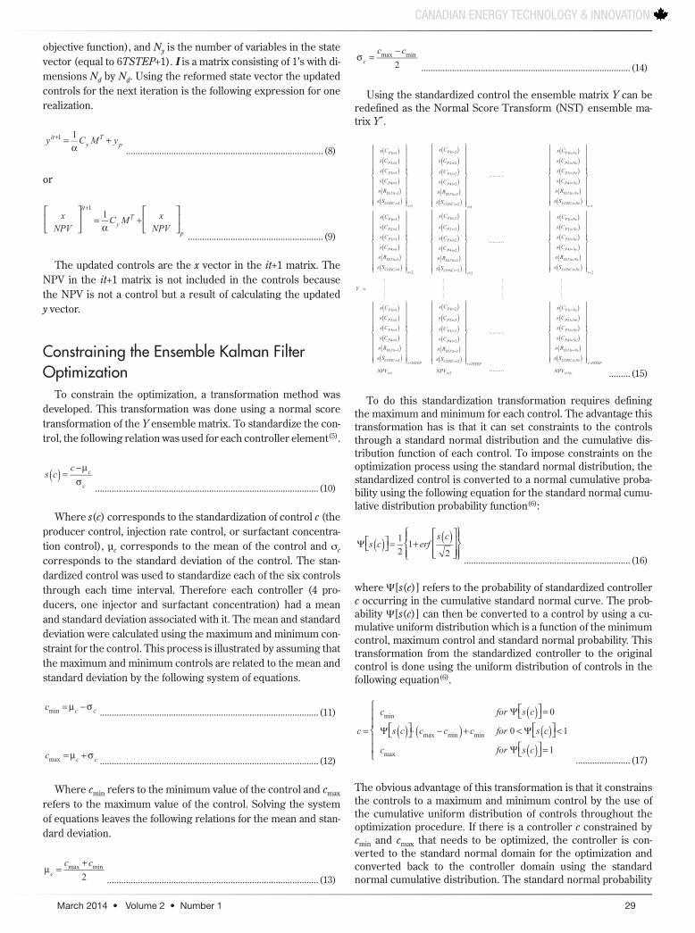
objective function), and Ny is the number of variables in the state vector (equal to 6TSTEP+1). I is a matrix consisting of 1’s with di-mensions Nd by Nd. Using the reformed state vector the updated controls for the next iteration is the following expression for one realization.

y C M y1it

yT

p1 =

α++

...................................................................................(8)

or

xNPV

C M xNPV

1it

yT

p

1

=

α+

+

.........................................................(9)

The updated controls are the x vector in the it+1 matrix. The NPV in the it+1 matrix is not included in the controls because the NPV is not a control but a result of calculating the updated y vector.

Constraining the Ensemble Kalman Filter Optimization

To constrain the optimization, a transformation method was developed. This transformation was done using a normal score transformation of the Y ensemble matrix. To standardize the con-trol, the following relation was used for each controller element(5).

s cc c

c( ) =

−µσ

..............................................................................................(10)

Where s(c) corresponds to the standardization of control c (the producer control, injection rate control, or surfactant concentra-tion control), μc corresponds to the mean of the control and σc corresponds to the standard deviation of the control. The stan-dardized control was used to standardize each of the six controls through each time interval. Therefore each controller (4 pro-ducers, one injector and surfactant concentration) had a mean and standard deviation associated with it. The mean and standard deviation were calculated using the maximum and minimum con-straint for the control. This process is illustrated by assuming that the maximum and minimum controls are related to the mean and standard deviation by the following system of equations.

c c cmin = µ − σ ............................................................................................(11)

c c cmax = µ + σ ............................................................................................(12)

Where cmin refers to the minimum value of the control and cmax refers to the maximum value of the control. Solving the system of equations leaves the following relations for the mean and stan-dard deviation.

c c

2cmax minµ =

+

.........................................................................................(13)

c c

2cmax minσ =

−

........................................................................................(14)

Using the standardized control the ensemble matrix Y can be redefined as the Normal Score Transform (NST) ensemble ma-trix Y*.

Y

s C

s C

s C

s C

s R

s S

s C

s C

s C

s C

s R

s S

s C

s C

s C

s C

s R

s S

s C

s C

s C

s C

s R

s S

s C

s C

s C

s C

s R

s S

s C

s C

s C

s C

s R

s S

s C

s C

s C

s C

s R

s S

s C

s C

s C

s C

s R

s S

s C

s C

s C

s C

s R

s S

NPV NPV NPV

P i

P i

P i

P i

INJ i

CONCit

P i

P i

P i

P i

INJ i

CONCit

P i Ne

P i Ne

P i Ne

P i Ne

INJ i Ne

CONCi Net

P i

P i

P i

P i

INJ i

CONCit

P i

P i

P i

P i

INJ i

CONCit

P i Ne

P i Ne

P i Ne

P i Ne

INJ i Ne

CONCi Net

P i

P i

P i

P i

INJ i

CONCit TSTEP

P i

P i

P i

P i

INJ i

CONCit TSTEP

P i Ne

P i Ne

P i Ne

P i Ne

INJ i Ne

CONCi Net TSTEP

i i i Ne

1 1

2 1

3 1

4 1

1 1

11

1 2

2 2

3 2

4 2

1 2

21

1

2

3

4

1

1

1 1

2 1

3 1

4 1

1 1

12

1 2

2 2

3 2

4 2

1 2

22

1

2

3

4

1

2

1 1

2 1

3 1

4 1

1 1

1

1 2

2 2

3 2

4 2

1 2

2

1

2

3

4

1

1 2

��

��

��

��

��

��

��

��

( )

( )

( )

( )( )( )( )( )( )

( )

( )( )( )( )

( )( )( )( )( )( )

( )( )( )( )( )( )

( )

( )( )( )( )

( )( )( )( )( )( )

( )( )( )( )( )( )

( )

( )( )( )( )

( )( )( )( )( )( )

=

�

�

��

�

�

��

�

=

=

=

=

=

==

=

=

=

=

=

==

=

=

=

=

=

==

=

=

=

=

=

==

=

=

=

=

=

==

=

=

=

=

=

==

=

=

=

=

=

==

=

=

=

=

=

==

=

=

=

=

=

==

= = = .........(15)

To do this standardization transformation requires defining the maximum and minimum for each control. The advantage this transformation has is that it can set constraints to the controls through a standard normal distribution and the cumulative dis-tribution function of each control. To impose constraints on the optimization process using the standard normal distribution, the standardized control is converted to a normal cumulative proba-bility using the following equation for the standard normal cumu-lative distribution probability function(6):

s c erfs c1

21

2( ) ( )

Ψ = +

......................................................................(16)

where Ψ[s(c)] refers to the probability of standardized controller c occurring in the cumulative standard normal curve. The prob-ability Ψ[s(c)] can then be converted to a control by using a cu-mulative uniform distribution which is a function of the minimum control, maximum control and standard normal probability. This transformation from the standardized controller to the original control is done using the uniform distribution of controls in the following equation(6).

c

c for s c

s c c c c for s c

c for s c

0

0 1

1

min

max min min

max

( )( ) ( ) ( )

( )=

Ψ =

Ψ ⋅ − + < Ψ <

Ψ =

.......................(17)

The obvious advantage of this transformation is that it constrains the controls to a maximum and minimum control by the use of the cumulative uniform distribution of controls throughout the optimization procedure. If there is a controller c constrained by cmin and cmax that needs to be optimized, the controller is con-verted to the standard normal domain for the optimization and converted back to the controller domain using the standard normal cumulative distribution. The standard normal probability

30 www.ceti-mag.ca


is used to determine the controller’s value using the uniform cu-mulative distribution of the controller. This process is conveyed in Figure 3 and illustrates that a new standardized controller, z, was obtained through the optimization process and converted from the standard normal domain to the controller domain using the uniform cumulative distribution curve of the control which is bounded by cmin=5 and cmax=20.

The transformed matrix is used to advance the controls for the next iteration, therefore the previously mentioned average Y matrix, Cy matrix, and yit+1 vector are based on the transformed matrix. The calculation of the transformed average Y matrix, transformed Cy matrix and transformed yit+1 vector based on a transformed Y matrix is illustrated in the following series of equations.

YNe

x

NPV

1i

i

Ne

ii

Ne

1

1

∑

∑=

∗

∗

=

= ................................................................................(18)

CNe

Y Y Y Y11y

T*( )( )=

−− −∗ ∗ ∗ ∗

................................................................(19)

y C M y1it

yT

p1 =

α+( )+ ∗ ∗

∗

..............................................................................(20)

xNPV

C M xNPV

1it

yT

p

1

=

α+

+

....................................................... (21)

The superscript, *, indicates that the matrix or vector is trans-formed. To use the controls in the simulator, the transformed vector is converted back to the controller domain using the pre-viously mentioned transformation procedures. The conversion from the controller domain, Y, to the transformed domain, Y*, is used to perform the update of the controls with user defined con-straints for every ensemble member. However, this transforma-tion however is done once in the beginning of the optimization routine on the original Y matrix (Figure 4). The conversion from the transformed domain, Y*, to the controller domain, Y, is used

0%

10%

20%

30%

40%

50%

60%

70%

80%

90%

100%

-6 -4 -2 0 2 4 6

Prob

abili

ty

s(c) = (x-µc)/σc

Standard Normal Cumulative Distribution Curve

0%

10%

20%

30%

40%

50%

60%

70%

80%

90%

100%

0 5 10 15 20 25

Prob

abili

ty

c

Control c Uniform Cumulative Distribution Curve

z = s(c)

Ψ[s(c)] c c min

c max

Standard Domain Controller Domain

FIGURE 3: Normal transformation of controls from the standard normal cumulative curve (which is defined by µc and σc) to the uniform cumulative distribution curve (which is defined by cmin and cmax. Conversion between controls is dictated by user defined cmin and cmax.

FIGURE 4: Optimization program flow chart. The optimization process terminates when the average NPV for all of the ensemble members has stopped increasing.



to run the simulator with the updated set of controls for every ensemble member (x1 to xNe). This transformation is performed when a new Y* is determined using the optimization routine.

Determination of Weighting FactorThe non-adjoint optimization method used is a steepest as-

cent method in which CyMT serves as the gradient and the weighting factor serves as the direction of the gradient. The key to this method is adequately finding the direction of the gra-dient that maximizes the NPV for the iteration efficiently. If the initial weighting factor and step size is inadequate it may take a very long time to search for the optimal alpha that adequately maximizes the NPV. To exacerbate this problem, if the initial weighting factor is not large enough, one may never reach the optimal NPV because its optimal is much larger than the initial weighting factor. In addition, a large weighting factor may result in many optimization iterations while a small alpha may cause spurious results and overrun the controls out of their bounds and terminate the optimization iteration early. To address these prob-lems a new approach is used to find the weighting factor.

A robust weighting factor algorithm contains specific proper-ties. The first property is that it must be quick in approximately converging on an optimal alpha. The second property is that it must be able to shut off after a set number of iterations. The third property is that it must have a convergence error. The Gold-Sec-tion Search method(7) encompasses these characteristics. This method is a general single variable search that relies on the con-cept of the golden ratio(7). The golden ratio, R, is conveyed in the following relation.

R5 12

= −

................................................................................................(22)

The golden ratio is used to make the golden section search algorithm approach rapidly to an answer. The Golden-Section Search is implemented by first choosing two extreme guesses, alphalow and alphahigh, that bracket the optimal NPV or f(alpha). Two interior points, alpha1 and alpha2, are calculated using the golden ratio.

d R alpha alphahigh low( )= ⋅ −.....................................................................(23)

alpha alpha d1 low= + ................................................................................(24)

alpha alpha d2 high= −...............................................................................(25)

The simulator is then run to determine both f(alpah1) and f(alpha2). Note, f(alpha) consists of running the simulator for con-trols x1 through xNe and averaging the NPV across each ensemble member. Two things may happen once this is done.

1. f(alpah1) > f(alpha2) then the domain of alpha to the left of alpha2 from alphalow to alpha2 is eliminated because it does not contain the maximum. Then the intervals are redefined as the following:

alpha alphalow 2,old= .................................................................................(26)

alpha alpha ,old2 1= ....................................................................................(27)

alpha alpha R alpha alphalow high low1 ( )= + ⋅ −............................................(28)

which results in f(alpha2)= f(alpah1) and f(alpah1) is deter-mined by utilizing the simulator.

2. f(alpah2) > f(alpha1) then the domain of alpha to the right of alpha1 from alphahigh to alpha1 is eliminated because it does not contain the maximum. Then the intervals are redefined as the following:

alpha alphahigh ,old1=.................................................................................(29)

alpha alpha ,old1 2= ....................................................................................(30)

alpha alpha R alpha alphahigh high low2 ( )= − ⋅ − ..........................................(31)

which results in f(alpha1)= f(alpah2) and f(alpah2) is deter-mined by utilizing the simulator.

Once the first or second conditions are satisfied, the new in-terval is defined using the following possible conditions.

3. (alpah1) > f(alpha2) then alphaopt=alpha1 and f(alphaopt)=f(alpha1).

4. f(alpah2) > f(alpha1) then alphaopt=alpha2 and f(alphaopt)=f(alpha2).

The conditions 1 through 4 are repeated until convergence or until a minimum error is achieved which is represented by the following expression.

e Ralpha alpha

alpha1 100%a

high low

opt( )= − ⋅

−⋅

..................................................(32)

This expression provides a condition in which the algorithm is terminated. The power of the Golden Section Search method is that the interval containing the optimal alpha is reduced rap-idly. Each iteration to find the optimal alpha results in the interval being reduced by a factor of the golden ratio or 61.8%(9 7). In this work, the maximum alpha, minimum alpha, maximum number of iteration until termination and the maximum error allowed were 1010, 1,000, 100 and 50%, respectively.

Defining the Initial ControlsTo initiate the optimization, it is important to define the initial

ensembles of the control vector x. Multiple ensembles of control vector x have to be created because the optimization method re-quires that a covariance matrix, Cy, be calculated. The covariance matrix represents the deviation between each ensemble of con-trol x and the mean control x. Multiple ensembles of the control x cannot all be identical because it would indicate a covariance ma-trix filled with zeroes. These zeroes would terminate the optimi-zation prematurely because of no gradient for the steepest ascent.

The design of the prior ensembles of the 5 spot surfactant flood field is important when using the Ensemble Kalman Filter optimi-zation technique. When the Ensemble Kalman Filter is used as

32 www.ceti-mag.ca


a history match tool to match permeability to observations such as bottomhole pressure, the initial ensemble of permeability is routinely taken from a distribution of permeability based on em-pirical data in the field. As a corollary to history matching, the dis-tribution of the ensemble of initial controls should also be based on physical laws in petroleum engineering. This work addresses these concerns in the design of the initial prior for the Ensemble Kalman Filter optimization process for the total liquid production rate control of the producer wells scenario and bottomhole pres-sure control of the producer wells scenario. Both scenarios also include the control of liquid injection rate and control of injected surfactant concentration as suggested by Equation 1. A few as-sumptions were made concerning the design of the initial prior. These assumptions include the following.

1. Transient response when the well first opens and also when the well changes controls. This assumption covers the re-sponse in which the wells have not felt the pressure bound-aries yet due to non-boundary dominated flow.

2. Ideal design is when the reservoir pressure is close to the initial reservoir pressure at all times during production.

3. Controls are held constant from one user given time interval until the next time interval. Therefore the controls are es-sentially stepwise.

Total Liquid Production Rate Control of the ProducerThe total liquid production rate control is based on conven-

tional decline curve analysis and the assumption that, for this case of control, the well has not felt its boundaries. Decline curve analysis attempts to find the ‘best fit’ curve that matches the pro-duction data and forecasts this curve for future economic produc-tion. But to serve the purpose of having a covariance matrix for the optimization method, decline curve analysis was used to gen-erate multiple realizations of the liquid rate. The decline curve type that was used in this paper was the hyperbolic decline cure. This decline curve was chosen because changing the liquid pro-duction rate to different values during the production life implies that the well never feels its boundaries and thus exhibits tran-sient behaviour. For this paper, only the beginning of the time in-terval was available for the control (control is constant between different time intervals). Therefore, the hyperbolic decline equa-tion was altered to account for this control. The modified liquid control case equation is the following expression.

q t Qb D t T

11

365initinit

b1/

( ) ( )= ⋅ +

⋅ ⋅ − ⋅ ∆

−

...................................................(33)

The Qinit represents the initial production rate at the start of the production, Dinit is the initial decline rate at the start of the production, t is the time interval through the production life, ∆T stands for the length of the time interval, and b stands for a factor that describes whether the well is in boundary or non-boundary dominated flow. Values of b from 0 to 1 are associated with boundary dominated flow, while values greater than 1 are associated with non-boundary dominated flow or transient well behaviour. Typically when using decline curve analysis to curve fit production history the Qinit, Dinit and b terms are fit used using a least square analysis. The Qinit, Dinit and b terms for this work were varied by first creating realizations of these parameters and then sampling from the distribution of these parameters to create realizations of hyperbolic decline throughout the production time. The following equations illustrate the uniform distribution of realizations of Qinit, Dinit and b.

Q RN Q -Q Qiniti

initMax

initMin

initMin( )= ⋅ +

...............................................................(34)

D RN D -D Diniti

initMax

initMin

initMin( )= ⋅ +

..............................................................(35)

b RN b -b bi Max Min Min( )= ⋅ + .......................................................................(36)

The Max superscript indicates the maximum for the param-eter, RN stands for a random number between 0 and 1, Min stands for minimum, and i indicates the ith realization. The pre-ceding set of equations was used to generate realizations for wells P1, P2, P3 and P4.

Bottomhole Pressure Control of the ProducerAs mentioned earlier, changing the controls prevents the wells

from feeling the boundaries. As a result of this, the bottomhole pressure control was based on the transient inflow performance relationship. This relationship is the following expression(8).

q tkh P BHP

BT t

k

c r12.3012log 24 log

74.21463.23i

t w2

1

( ) ( ) ( )=−

µ∆ ⋅ ⋅ +

ϕµ

−

−

...............(37)

where Pi is the initial reservoir pressure in kPa, BHP is the bot-tomhole flowing pressure in kPa, B is the oil formation volume factor, µ is the oil viscosity in cP, h is the net pay in m, ct is the total compressibility in kPa-1, k is the permeability in mD, and rw is the inner radius of the well in m. To use the transient flow equation, the transient productivity index was derived from the transient inflow performance relationship. This relation is the following ex-pression where J is the productivity index.

Jq

P BHP

khB

T tk

c r12.3012log 24 log

74.21463.23

i t w2

1

( ) ( )=−

=µ

∆ ⋅ ⋅ +ϕµ

−

−

......(38)

This productivity index was modified to account for the step-wise change in controls. The productivity index was altered to account for control at the beginning of the timestep and the first hour of change. This change is expressed in the following equations.

Jq

P BHP

khB

tk

c r12.3012log log

74.21463.23

ie

t w2

1

( ) ( )=−

=µ

+ϕµ

−

−

.............(39)

t T t 1 24 1e ( )= ∆ ⋅ − ⋅ +.................................................................................(40)

In an undersaturated oil reservoir there are primarily two phases flowing at any time, thus the total productivity index was split into a water and oil phase productivity indexes. This phase breakdown is illustrated in the following expression.



J tk k h

Bt

k k

c r

k k h

Bt

k k

c r

12.3012log log

74.21463.23

12.3012log log

74.21463.23

Tro

o oe

ro

t w

rw

w we

rw

t w

2

1

2

1

( ) ( )

( )

=⋅ ⋅

µ+

⋅

ϕµ

−

+

⋅ ⋅µ

+⋅

ϕµ

−

−

−

...............(41)

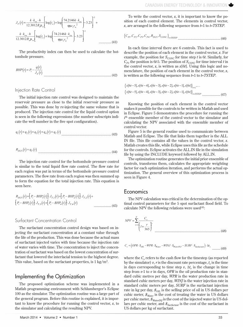
The productivity index can then be used to calculate the bot-tomhole pressure.

BHP t Pq t

J tiT

( ) ( )( )= −

.................................................................................(42)

Injection Rate ControlThe initial injection rate control was designed to maintain the

reservoir pressure as close to the initial reservoir pressure as possible. This was done by re-injecting the same volume that is produced. The injection rate control for the liquid control option is seen in the following expressions (the number subscripts indi-cate the well number in the five spot configuration).

q t q t q t q t q tT1 2 3 4( ) ( ) ( ) ( ) ( )+ + + =............................................................(43)

R t q tINJ T1 ( ) ( )= ........................................................................................(44)

The injection rate control for the bottomhole pressure control is similar to the total liquid flow rate control. The flow rate for each region was put in terms of the bottomhole pressure control parameters. The flow rate from each region was then summed up to form the equation for the total injection rate. This equation is seen here.

R t P BHP t J t P BHP t J t

P BHP t J t P BHP t J t

INJ i T i T

i T i T

1 1 ,1 2 ,2

3 ,3 4 ,4

( ) ( ) ( ) ( ) ( )( ) ( ) ( ) ( )

= − ⋅ + − ⋅ +

− ⋅ + − ⋅.....................(45)

Surfactant Concentration ControlThe surfactant concentration control design was based on in-

jecting the surfactant concentration at a constant value through the life of the production. This was done because the actual mass of surfactant injected varies with time because the injection rate of water varies with time. The concentration to inject the concen-tration of surfactant was based on the lowest concentration of sur-factant that lowered the interfacial tension to the highest degree. This value, based on the surfactant properties, is 1 kg/m3.

Implementing the OptimizationThe proposed optimization scheme was implemented in a

Matlab programming environment with Schlumberger’s Eclipse 100 as the simulator. The optimization routine was a large part of the general program. Before this routine is explained, it is impor-tant to know the procedure for running the control vector, x, to the simulator and calculating the resulting NPV.

To write the control vector, x, it is important to know the po-sition of each control element. The elements in control vector, x, are arranged in the following sequence from t=1 to t=TSTEP.

C C C C R S C C C C R S, , , , , , , , , , , ,P P P P INJ CONC t P P P P INJ CONC t TSTEP1 2 3 4 1 1 1 2 3 4 1…{ } { }= = ...................................................(46)

In each time interval there are 6 controls. This fact is used to describe the position of each element in the control vector, x. For example, the position for SCONC for time step t is 6t. Similarly, for CP1 the position is 6t-5. The position of SCONC for time interval t in the control vector, x, is written as x[6t]. Using this logic and no-menclature, the position of each element in the control vector, x, is written as the following sequence from t=1 to t=TSTEP.

x t x t x t x t x t x t

x t x t x t x t x t x t

[6 5], [6 4], [6 3], [6 2], [6 1], [6 ] ,

[6 5], [6 4], [6 3], [6 2], [6 1], [6 ]t

t TSTEP

1…{ }

{ }− − − − −

− − − − −=

= ......................(47)

Knowing the position of each element in the control vector makes it possible for the controls to be written in Matlab and used in Eclipse. Figure 5 demonstrates the procedure for running the ith ensemble member of the control vector to the simulator and calculating the NPV associated with the ensemble member of control vector.

Figure 5 is the general routine used to communicate between Matlab and Eclipse. The file that links them together is the ALL.IN file. This file contains all the values in the control vector, x. Matlab creates this file, while Eclipse uses this file as the schedule for the controls. Eclipse activates the ALL.IN file in the simulation file by using the INCLUDE keyword followed by ALL.IN.

The optimization routine generates the initial prior ensemble of controls, transforms them, calculates the appropriate weighting factor for each optimization iteration, and performs the actual op-timization. The general overview of this optimization process is seen in Figure 4.

EconomicsThe NPV calculation was critical in the determination of the op-

timal control parameters for the 5 spot surfactant flood field. To calculate NPV the following relations were used(4):

NPVC

1r365

vt

v 1

V

v∑=

+

=

...............................................................................(48)

C OPR $ WPR $ WINJ $ SURF $ tv OIL Water WaterINJ Surfactant v( )= ⋅ − ⋅ − ⋅ − ⋅ ⋅ ∆ ..........(49)

where the Cv refers to the cash flow for the timestep (as reported by the simulator) v, r is the discount rate percentage, tv is the time in days corresponding to time step v, ∆tv is the change in time step from v-1 to v in days, OPR is the oil production rate in stan-dard cubic metres per day, WPR is the water production rate in standard cubic meters per day, WINJ is the water injection rate in standard cubic meters per day, SURF is the surfactant injection rate in kg per day, $OIL is the selling price of oil in US dollars per cubic meter, $Water is the cost of treating the water in US dollars per cubic meter, $WaterINJ is the cost of the injected water in US dol-lars per cubic meter, and $Surfactant is the cost of the surfactant in US dollars per kg of surfactant.

34 www.ceti-mag.ca


NPV is a measure of a project’s success. A positive NPV in-dicates that the project pays for its own cost, while a negative NPV indicates that the project does not generate enough income to sustain itself financially(9). It is important to note that the eco-nomic parameters of oil price, surfactant cost, water injection cost and water treatment cost are set constant for one NPV calcula-tion. This is a reasonable assumption because the NPV accounts for the interest earned during the project(9). Therefore, it is in-correct to change the economic parameters during the life of the project if the NPV is used only to screen the success of the project during its life.

Once the optimal solution was obtained, several realizations of the economic parameters (oil price, surfactant cost, water in-jection cost and water treatment cost) were used along with re-alizations of the permeability field to account for every possible

scenario. To do this, a triangular distribution of the economic parameters was used to create possible realizations of the eco-nomic parameters. Triangular distribution requires a most likely value or mode (TrM), a minimum value (TrL), and a maximum value(TrH). The triangular distribution depends on the magni-tude of the random number, RN, which is between 0 and 1. For different cases of the random number, the triangular distribu-tion(10) is the following equation for an economic parameter, Tr.

Tr

Tr Tr -Tr Tr Tr RN for RNTr -Tr

Tr Tr

Tr Tr -Tr Tr Tr 1 RN for RNTr -Tr

Tr Tr

L M L H LM L

H L

H H M H LM L

H L

( ) ( ) ( )( )

( ) ( ) ( ) ( )( )

=

+ ⋅ − ⋅ ≤−

− ⋅ − ⋅ − ≥−

........(50)

Table 1 contains the economic values used in this work.The discount rate percentage, r, was set constant at 10%. The

optimization routine uses the mode economic parameters, while the Monte Carlo sampling uses the realizations of all the eco-nomic parameters which are based on the triangular distribution.

Monte Carlo of Geological and Economic Realizations

Realizations of permeability and economic parameters were used to generate a picture of the probability of success using the optimal control once the optimization was completed using the mean permeability field, mean porosity field and the mode of the oil price. This was done by sampling every possible scenario of the permeability field and the economic parameters. This pro-cess is understood by envisioning Rk realizations of permeability fields, Rop realizations of oil price, Rwi realizations of injection cost, Rwt realizations of water treatment cost and Rsurf realizations of surfactant cost. The sampling process was accomplished by first generating the first scenario which is the 1st realization of perme-ability field, 1st realization of oil price, 1st realization of water injec-tion cost, 1st realization of water treatment cost and 1st realization of surfactant cost. After sampling the first scenario, the second

FIGURE 5: Matlab program flowchart to run control vector xi in Eclipse. Producer controls for wells P1, P2, P3 and P4 are written to file PRO_CONTROLSt.IN for time interval t. Injector controls for the injector well are written to INJ_CONTROLSt.IN for time interval t. Surfactant concentration for the injector well is written to CONC_CONCTROLSt.IN for time interval t.

TABLE 1: Economic parameters for triangular distribution.Economic Parameter Mode Minimum Maximum

Oil price ($/m3) 440 126 755Water treatment cost ($/m3) 12.58 6.29 18.87Water injection cost ($/m3) 6.29 4.40 12.58Surfactant price ($/kg) 2.20 1.76 3.31

TABLE 2: Reservoir and simulation properties used for main optimization studies. Property Property Value

Net pay 21.3 m Reservoir pressure 31,000 kPa Area 320 acre Top depth 3,048 ft Grid dimensions 50 x 50 x 1

∆X=22.7596 m Grid block size ∆Y=22.7596 m ∆Z=21.336 m

Formation compressibility 7.25E-7 kPa-1

Water compressibility 4.35E-7 kPa-1

Water viscosity 1 cp Water density 1,000 kg/m3

Water formation volume factor 1 Rm3/Sm3

Oil viscosity 3 cp Oil density 897 kg/m3

Oil formation volume factor 1 Rm3/Sm3



scenario would then be the 1st realization of permeability field, 1st realization of oil price, 1st realization of water injection cost, 1st re-alization of water treatment cost and 2nd realization of surfactant cost. This process would then be repeated until all scenarios are sampled for all realizations of permeability and economic param-eters. If all possible realizations are sampled, then there would be RkRopRwiRwtRsurf number of possible scenarios. Once the Monte Carlo sampling was finished, the cumulative probability plot of the NPV was created using a cumulative distribution plot (prepro-grammed in Matlab).

The cumulative probability plot of NPV has on its vertical axis cumulative probability, and NPV on its horizontal axis. It is impor-tant to understand the interpretation of this plot. If, at the mode economic parameters, the NPV is positive at a corresponding probability, Pmode, but at probabilities less than Pmode the NPV is negative, it means that the project is not successful for economic scenarios worse than the mode economic parameters. The cumu-lative probability plot of NPV is a measure of the project’s success for a given range of economic climate at the start of the project. The project success should not be taken as a failure if the NPV is shown to be negative for cumulative probabilities less than Pmode because the project has shown success using the mode economic scenarios.

Computing RequirementsThe optimization and incorporation of uncertainty in the eco-

nomics and permeability field requires many simulation runs. To generate the initial prior ensemble matrix, Y, it takes Ne simula-tion runs in Eclipse. To determine the proper weighting factor it takes at least three Ne simulation runs. To perform the opti-mization, it takes at least two optimization runs. To perform the Monte Carlo simulation, it takes Rk actual simulation runs and RkRopRwiRwtRsurf calculations of NPV. The graphics section of the program requires two Ne simulation runs to get the observa-tions using the original and optimized control for each ensemble member of control. The time it takes to run one simulation is ap-proximately 9 seconds. The time it takes to calculate 100 NPV (for Monte Carlo) is approximately 9 seconds. In total, the necessary time it takes for the entire program to finish is expressed in the following equation.

q Time hoursNe Ne Ne R R R R R R

Re . ( )9 2 3 2

9100

60 60

k k op wi wt surf( )≥

⋅ + ⋅ ⋅ + ⋅ + + ⋅ ⋅ ⋅ ⋅ ⋅ ⋅ ........(51)

The computer used was an Intel Core 2 Quad CPU with 2.66 GHz for each core and 3.25 GB of RAM. The “Req. Time (hours)” expression can be used to plan required optimization time using the CPU for this work.

Results and DiscussionExample Problem

The optimization method developed in this paper was applied to a two-dimensional surfactant and waterflood in a reservoir sim-ulator setting. The purpose is to illustrate the use of this method to optimize an EOR process defined in a simulator. Tables 2 to 7 provide simulation settings, surfactant properties and field data. Surfactant properties were chosen to illustrate a simple surfac-tant system where miscibility develops dynamically and is mod-elled using the simulator’s relative permeability model. The relative permeability model is an evolution from a Brooks Corey immiscible relative permeability curve at low capillary number to miscible relative permeability curve at high capillary number(11,

12). The miscible relative permeability relationship is based on ob-servations noted in the literature which show for a low interfacial tension system that the relative permeability to oil is large com-pared to the relative permeability to oil in a high interfacial ten-sion system(13). The water saturation was set at 40% and the life of the flood was set at 20 years with 6 month control change inter-vals. A total of 40 ensemble members (Ne) were used to create the ensemble matrix so as to match current practices of using 40 ensemble members for history matching. For this example, bot-tomhole pressure control of the producers was used for a surfac-tant flood optimization. Tables 8 and 9 are the DCA parameters

TABLE 8: DCA Parameters for optimization.DCA Parameter Mean Minimum Maximum

Qinit (Sm3/day) 160 16.0 302b 5 1 9Dinit (1/year) 5 0.1 9.9

TABLE 9: Constraints for 20 year surfactant and waterflood optimization.

Control Minimum Maximum

Bottom hole pressure (kPa) 345 31,000Injection rate (Sm3/day) 6.36 636Surfactant concentration (kg/m3) 0.0285 28.5

TABLE 3: Surfactant viscosity. Surfactant Concentration Viscosity (kg/m3) (cp) 0 1 30 5

TABLE 4: Capillary number. Log Capillary State of Fluid Number Interaction -9 Immiscible -4.5 Immiscible -2 Miscible 10 Miscible

TABLE 6: Surfactant adsorption. Surfactant Adsorption Concentration (kg surfactant/ (kg/m3) kg reservoir rock) 0 0 1 0.0005 30 0.0005

TABLE 7: Well properties. Center Well Name Grid Location Well Radius Completion and Type (X,Y,Z) (m) Depth (m) P1, 1st producer location (1,1,1) 0.244 3,059 P2, 2nd producer location (1,50,1) 0.244 3,059 P3, 3rd producer location (50,50,1) 0.244 3,059 P4, 4th producer location (50,1,1) 0.244 3,059 INJ1, injector location (25,25,1) 0.244 3,059TABLE 5: Surfactant surface tension.

Surfactant Surface Concentration Tension (kg/m3) (N/m) 0 0.05 1 1E-06 30 1E-06

36 www.ceti-mag.ca


NPV Distribution of Surfactant Flood Using BHP Control for 20 Years

$35,000,000

$30,000,000

$25,000,000

$20,000,000

$15,000,000

$10,000,000

$5,000,000

$01 2 3 4 5 6 7 8 9 10 11 12 13 14 15 16 17 18 19 20 21 22 23 24 25 26 27 28 29 30 31 32 33 34 35 36 37 38 39 40

Realization #Original Optimized

FIGURE 6: NPV distribution of 20 year surfactant flood. The producer control option was bottom hole pressure.

Cumulative Oil Distribution of Surfactant FloodUsing BHP Control for 20 Years

500,000

450,000

400,000

350,000

300,000

250,000

200,000

150,000

100,000

50,000

01 2 3 4 5 6 7 8 9 10 11 12 13 14 15 16 17 18 19 20 21 22 23 24 25 26 27 28 29 30 31 32 33 34 35 36 37 38 39 40

Realization #Original Optimized

FIGURE 7: Cumulative oil distribution of 20 year surfactant flood. The producer control option was bottom hole pressure.

Original Well P1 BHP Profile for all 40 Realizations Original Well P1 BHP Profile for all 40 Realizations31,200

31,000

30,800

30,600

30,400

30,200

30,000

29,800

29,600

29,400

26,200

26,100

26,000

25,900

25,800

25,700

25,600

25,500

25,400

kPa

kPa

0 50 100 150 200 250 0 50 100 150 200 250Time (months) Time (months)

(a) (b)

FIGURE 8: Well P1 controls for 20 year surfactant flood: a) original; b) optimized. Each colour represents a different realization of the Well P1 control (40 realizations total). The range of variability among the realizations is reduced from the original to the optimized.

kPa

31,000

30,000

29,000

28,000

27,000

26,000

25,000

24,000

23,000

22,000

21,000

Original Bottom Hole Pressure Profile for Realization #1 Original Bottom Hole Pressure Profile for Realization #1

(a) (b)

26,000

25,000

24,000

23,000

22,000

21,000

20,000

19,000

kPa

kPa

0 50 100 150 200 250

Time (months) Time (months)0 50 100 150 200 250

P1P2P3P4

P1P2P3P4

FIGURE 9: 1st realization of Well P1 controls for 20 year surfactant flood: a) original; b) optimized. Trends that existed in the original controls were maintained in the optimized controls while remaining within the user defined constraints.



used to create the initial Y ensemble matrix and the constraints of the flooding process.

Utilizing the developed optimization approach resulted in varying degrees of improvement in the NPV and cumulative oil across each ensemble member and is a result of the variability that exists in the original and optimized controls (Figures 6 and 7).

The original controls and optimized controls each have 40 re-alizations with a certain degree of variability. The optimization of the controls generally reduces the variability that exists in the original controls. This observation is seen in the Figure 8 for the bottomhole pressure control of Well P1.

The variability reduction is portrayed by the reduction in the range of the control through time. Though 40 realizations were used to do the optimization, it is only necessary to use one real-ization (Figures 9 and 10) to closely understand the effectiveness of this unique optimization routine.

From observing the 1st realization, it is apparent that the trends that existed in the original controls were maintained in the optimized controls while remaining within the user-defined con-straints. This has important consequences when defining other EOR processes. The optimization method developed in this paper results in the ability to maintain the trends that existed in the original controls and was able to translate those trends to the op-timized controls while obeying user-defined constraints.

Optimization results also reveal improvements to the field oil saturation due to the surfactant flood. Figure 11 illustrates that the optimized surfactant flood reduced the oil saturation to a higher degree than a waterflood that underwent the same optimi-zation process. Close examination indicates that the optimization forced the surfactant flood to sweep zones corresponding to high permeability (see Figure 12 for permeability field). These swept zones show significant reductions in oil saturation when com-pared to a waterflood that underwent the same optimization pro-cess. Given that the optimization’s goal was to improve NPV, this reveals that ideal economic conditions correspond to sweeping these high permeability zones. This is in contrast to the water-flood option that shows moderate reduction in oil saturation.

A comparison of the NPV and oil produced for the optimized surfactant and waterfloods show the advantage of optimized sur-factant EOR. The optimized waterflood resulted in production of .232 MMSm3 of oil and an NPV of 17.6 MM$. The optimized sur-factant flood resulted in a production of .426 MMSm3 of oil and an NPV of 31.3 MM$. For NPV, the optimized surfactant flood shows an improvement of 78% over the optimized waterflood. For oil pro-duced, the optimized surfactant flood shows an improvement of 84% over the optimized waterflood.

NPV is an indicator of how well the EOR process can add value. The cumulative distribution curve is a ranking of the possible sce-narios incorporating permeability and economics. The cumula-tive distribution curve generated as a result of the sampling of

Injection Rate Profile for Realization #1 Injected Surfactant Concentration Profile for Realization #1

(a) (b)

800

700

600

500

400

300

2000 50 100 150 200 250

Time (months) Time (months)0 50 100 150 200 250

OptimizedOriginal

kg/m

3

7

6

5

4

3

2

1

0

OptimizedOriginal

FIGURE 10: 1st Realization of injection rate control and surfactant concentration control for 20 year surfactant flood: a) injection rate control; b) surfactant concentration control.

FIGURE 11: Comparison between 1st realization of optimized 20 year floods: a) waterflood; b) surfactant flood.

38 www.ceti-mag.ca


permeability fields and economic parameters (Figure 13) is an indication of the possible NPVs that can occur if a set of perme-ability field and economic parameters were implemented at the start of the project. This means that for the surfactant flood, 40% of the scenarios incorporating permeability and economics are worse than using the mode economic parameters and mean per-meability field. Although there are regions in the cumulative dis-tribution curve that are negative, these regions correspond to less favourable economics such as low oil price, expensive surfactant, expensive water injection cost and expensive water treatment cost. These negatives NPVs are not an indication of the failure of the project because using the mode economic parameters and mean permeability field results in a positive NPV. These negative NPVs represent a warning to have favourable economics to en-sure project success.

Computer Program TimeThe program written for the optimization process and the

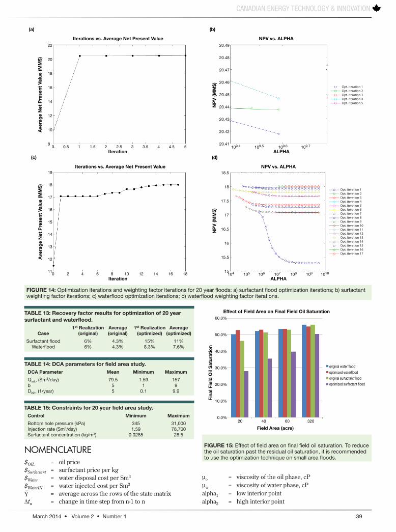
Monte Carlo sampling using the optimal solution took substantial time to run. Table 10 lists the run times, the number of optimi-zation iterations, the maximum number of weighting factor iter-ations and the minimum number of weighting factor iterations. The computer used was a Intel Core 2 Quad CPU with 2.66 GHz for each core and 3.25 gigabytes of memory.

The majority of the program time was devoted in determining the weighting factor “alpha” that gave the best average NPV for one optimization iteration. Each weighting factor iteration re-quired 40 ensemble members (40 simulation runs). The optimi-zation iterations along with the iterations to find the optimal alpha are illustrated in Figure 14.

ConclusionsThe newly developed method for optimization allows optimiza-

tion of a system with user defined constraints and initial controls defined by engineering judgment. Tables 11 to 13 show the re-sults of the waterflood and surfactant flood example optimization.

To further illustrate the utility of this method and to under-stand where this method is effective, a field study was conducted using the same permeability and porosity fields on the surfactant and waterflood for 20 years with 6 month control change. Tables 14 and 15 show the DCA parameters and constraints used in this study.

The results of the study illustrate that for the surfactant flood, the oil saturation is minimized for small areas (Figure 15). As a result of this analysis, a small field area must be used to maximize the potential effectiveness of the surfactant flood.

Conversion Factorspsi × 14.5038 = barbbl × 1.589873 E-01 = m3

lbm × 4.535924 E-01 = kgft3 × 2.831685 E-02 = m3

1

0.9

0.8

0.7

0.6

0.5

0.4

0.3

0.2

0.1

0

Rel

ativ

e Pe

rmea

bilit

y

0 0.2 0.4 0.6 0.8 1So

kro, IMMISCIBLE krw, IMMISCIBLE

kro, Ultra Low IFT krw, Ultra Low IFT

FIGURE 12: Immiscible and miscible relative permeability curves used for waterflood and surfactant flood.

Probabilistic NPV for Realization #11

0.9

0.8

0.7

0.6

0.5

0.4

0.3

0.2

0.1

0

Prob

abili

ty

-20 0 20 40 60 80 100

NPV, MM$

NPV using modeeconomic parametersand mean permeabilityfield = 31.3MM$Probability = 40%

FIGURE 13: Cumulative distribution curve for NPV for surfactant flood for production time of 20 years.TABLE 10: Optimization computer program time.

CPU Minimum Maximum Optimization Time Alpha Alpha Case Iterations (hours) Iterations Iterations

Surfactant flood 5 6.4 2 4 Waterflood 17 24.6 4 28

TABLE 11: NPV results for optimization of 20 year surfactant and waterflood. 1st Realization Average 1st Realization Average Increase in Increase in Case (original) (original) (optimized) (optimized) 1st Realization Average

Surfactant flood $12,400,000 $9,760,000 $31,300,000 $20,500,000 152% 110% Waterflood $14,800,000 $11,400,000 $17,600,000 $18,000,000 19% 57%

TABLE 12: Cumulative oil results for optimization of 20 year surfactant and waterflood. 1st Realization Average 1st Realization Average Increase in Increase in Case (original) (original) (optimized) (optimized) 1st Realization Average

Surfactant flood .168 MMSm3 .119 MMSm3 .426 MMSm3 .312 MMSm3 150% 160% Waterflood .167 MMSm3 .121 MMSm3 .232 MMSm3 .211 MMSm3 39% 74%



NOMENCLATURE$OIL = oil price$Surfactant = surfactant price per kg$Water = water disposal cost per Sm3

$WaterIN = water injected cost per Sm3

Y_ = average across the rows of the state matrix

∆tn = change in time step from n-1 to n

µo = viscosity of the oil phase, cPµw = viscosity of water phase, cPalpha1 = low interior pointalpha2 = high interior point

Iterations vs. Average Net Present Value NPV vs. ALPHA

(a) (b)

22

20

18

16

14

12

10

8 0. 0.5 1 1.5 2 2.5 3 3.5 4 4.5 5

Aver

age

Net

Pre

sent

Val

ue (M

M$)

Iterations vs. Average Net Present Value NPV vs. ALPHA

(c) (d)Iteration

19

18

17

16

15

14

13

12

110 2 4 6 8 10 12 14 16 18

Aver

age

Net

Pre

sent

Val

ue (M

M$)

Iteration

20.49

20.48

20.47

20.46

20.45

20.44

20.43

20.42

20.41109.4 109.5 109.6 109.7

NPV

(MM

$)

ALPHA

Opt. iteration 1Opt. iteration 2Opt. iteration 3Opt. iteration 4Opt. iteration 5

18.5

18

17.5

17

16.5

16

15.5

15104 105 106 107 108 109 1010

NPV

(MM

$)

ALPHA

Opt. iteration 1Opt. iteration 2Opt. iteration 3Opt. iteration 4Opt. iteration 5Opt. iteration 6Opt. iteration 7Opt. iteration 8Opt. iteration 9Opt. iteration 10Opt. iteration 11Opt. iteration 12Opt. iteration 13Opt. iteration 14Opt. iteration 15Opt. iteration 16Opt. iteration 17

FIGURE 14: Optimization iterations and weighting factor iterations for 20 year floods: a) surfactant flood optimization iterations; b) surfactant weighting factor iterations; c) waterflood optimization iterations; d) waterflood weighting factor iterations.

Effect of Field Area on Final Field Oil Saturation

Fina

l Fie

ld O

il Sa

tura

tion

60.0%

50.0%

40.0%

30.0%

20.0%

10.0%

0.0%

Field Area (acre)20 40 60 320

original water floodoptimized waterfloodoriginal surfactant floodoptimized surfactant flood

FIGURE 15: Effect of field area on final field oil saturation. To reduce the oil saturation past the residual oil saturation, it is recommended to use the optimization technique on small area floods.

TABLE 14: DCA parameters for field area study.DCA Parameter Mean Minimum Maximum

Qinit, (Sm3/day) 79.5 1.59 157b 5 1 9Dinit, (1/year) 5 0.1 9.9

TABLE 15: Constraints for 20 year field area study.Control Minimum Maximum

Bottom hole pressure (kPa) 345 31,000Injection rate (Sm3/day) 1.59 78,700Surfactant concentration (kg/m3) 0.0285 28.5

TABLE 13: Recovery factor results for optimization of 20 year surfactant and waterflood.

1st Realization Average 1st Realization Average Case (original) (original) (optimized) (optimized)

Surfactant flood 6% 4.3% 15% 11% Waterflood 6% 4.3% 8.3% 7.6%

40 www.ceti-mag.ca


alphahigh = high guess of alphaalphalow = low guess of alphab = Arps decline exponent factorBHP = bottomhole pressure, kPaBo = oil formation volume factorBw = water formation volume factorc = controlcmax = maximum value of control ccmin = minimum value of control c CP1 = control of production well P1CP2 = control of production well P2CP3 = control of production well P3CP4 = control of production well P4ct = total compressibility, kPa-1

Cv = cash flow for timestep v (as reported by the simulator)

Cx = covariance of control vectorCy = covariance of YDinit = initial decline rate at the start of the production∆T = length of the time interval, daysf(alpha) = average NPV across each ensembleG = sensitivity matrixg(x) = Net Present ValueG(xit) = sensitivity matrix at itth iterationh = net pay, mI = Identity matrixi = realization numberit = iteration numberJ = productivity index, Sm3/Day/kPaJo = oil phase productivity index, Sm3/Day/kPaJT = total productivity index, Sm3/Day/kPaJw = water phase productivity index, Sm3/Day/kPak = permeability, mDkro = relative permeability of the oil phasekrw = relative permeability to the water phase M = measurement operatorMax = maximumMin = minimumNd = number of measurementsNe = number of realizations for Ensemble Kalman FilterNe = total number of realizationsNPV = Net present valueNy = number of variables in the state vectorP = reservoir pressure, kPaPi = initial reservoir pressure, kPaq(t) = total production rate for time interval t, Sm3

Qinit = initial production rate at the start of the production, Sm3/Day

r = discount rate, %R = golden ratioRINJ1 = Injection rate of well INJ1, Sm3/DayRk = total realizations of permeability fieldsRN = random number in the range from 0 to 1Rop = total realizations of oil priceRsurf = total number of realizations of surfactant costrw = inner radius of the well, mRwi = total number of realizations of water injection costRwt = total number of realizations of water treatment costRΦ = total realizations of porosity fieldss(c) = the standardization of control c S(x) = objective functionSCONC = concentration of surfactant in the Injector, kg/Sm3

SURF = total amount of surfactant used, kgt = time interval through the production life

TrH = maximum of economic parameterTrL = minimum of economic parameterTrM = mode of economic parameterTSTEP = total number of time intervals tv = time in days corresponding to timestep v (as re-

ported by the simulator) vv = represents the timesteps from 0 to VV = total number of timestepsWINJ = total water injected, Sm3

WPR = total water production for time period, Sm3

x = control vectorxp = prior control vectorY = state matrixy = state vectoryp = prior estimate of yY* = normal score transformation of Y matrixα = weighting factor alphaμc = mean of control cσc = standard deviation of control cΦ = porosityΨ[s(c)] = the probability of standardized controller c occur-

ring in the normal cdf

REFERENCES 1. SUN, Y., Petroleum Geology - Lecture 17: Frontiers in Reservoir

Research; GEOL 603 Petroleum Geology, Texas A&M University De-partment of Geology & Geophysics, Spring Semester, 2009.

2. BARRUFET, M., Chemical Flooding Notes; PETE 609 Enhanced Oil Recovery Processes, Texas A&M University Department of Petroleum Engineering, Spring Semester, 2008.

3. LORENTZEN, R.J., BERG, A.M., NAEVDAL, G. and VEFRING, E.H., A New Approach for Dynamic Optimization of Waterflooding Problems; Paper SPE 99690 presented at the Intelligent Energy Con-ference and Exhibition, Amsterdam, The Netherlands, 11-13 April 2006.

4. NWAOZO, J., Dynamic Optimization of a Water Flood Reservoir; M.Sc. thesis, University of Oklahoma, Norman, OK, 2006.

5. MONTGOMERY, D.C. and RUNGER, G.C. Applied Statistics and Probability for Engineers; Fourth Edition, John Wiley & Sons, Hoboken, New Jersey, 2007.

6. JAFARPOUR, B., Reservoir Characterization and Forecasting - Topic 3: Review of Probability & Univariate Statistics; PETE 689 Reservoir Characterization and Forecasting, Texas A&M University Department of Petroleum Engineering, Fall Semester, 2008.

7. CHAPRA, S.C. and CANALE, R.P., Numerical Methods for En-gineers: With Software and Programming Applications; Fourth Edition, McGraw-Hill Publishing Co., New York, NY, 2002.

8. ECONOMIDES, M.J., HILL, A.D. and EHLIG-ECONOMIDES, C., Petroleum Production Systems; Prentice Hall, Upper Saddle River, New Jersey, 1993.

9. MIAN, M.A., Project Economics and Decision Analysis Volume I: Deterministic Models; PennWell Corporation, Tulsa, OK, 2002.

10. MIAN, M.A., Project Economics and Decision Analysis Volume II: Probabilistic Models; PennWell Corporation, Tulsa, OK, 2002.

11. SCHLUMBERGER SOFTWARE, Eclipse Reference Manual; Sch-lumberger, Houston, TX, 2008.

12. SCHLUMBERGER SOFTWARE, Eclipse Technical Description Manual; Schlumberger, Houston, TX, 2008.

13. CINAR, Y., MARQUEZ, S. and ORR JR., F.M., Effect of IFT Variation and Wettability on Three-Phase Relative Permeability; Paper SPE 90572 presented at the SPE Annual Technical Conference and Exhibi-tion, Houston, TX, 26-29 September 2004.

CETI-13-027. Modified Ensemble Kalman Filter Optimization of Surfactant Flood Under Economic and Geological Uncertainty. CETI April 2014 2(1): pp. 27-41. Submitted 23 October 2013; Revised 3 February 2014; Accepted 1 June 2014.


Uchenna Odi is a Research Scientist at ENI Petroleum and a Visiting Scientist at the Massachusetts Institute of Technology on behalf of ENI. He holds a B.S. degree in chemical engineering from the Univer-sity of Oklahoma, in addition to M.S. and Ph.D. degrees in petroleum engineering from Texas A&M University. His interests are in optimization algorithms, risk anal-ysis, emulsion systems, enhanced oil re-covery, CO2 Sequestration and reservoir fluids.

Robert Lane is Professor and Director of the Crisman Institute for Petroleum Re-search in the Harold Vance Department of Petroleum Engineering at Texas A&M University. His career includes academic and oil company research, as well as field experience in Prudhoe Bay Operations Engineering, ARCO Alaska, where he fo-cused on subsurface water and gas man-agement, a topic on which he has since lectured and consulted. In 2003, he was a Professor, and from 2004 - 2007 Program Director, of Petroleum Engineering at the Petroleum Institute in Abu Dhabi, UAE. Lane holds B.S. and Ph.D. degrees in chemistry from the Universities of North Carolina and Florida, respectively.

Dr. Maria A. Barrufet is a Professor in the Harold Vance Department of Petro-leum Engineering at Texas A&M Univer-sity and the holder of the Baker Hughes Chair. She is also the Director of the Dis-tance Learning Program in the Petroleum Engineering Department. Dr. Barrufet is an expert in compositional modelling. She has developed fluid models for composi-tional simulation from near-critical fluids, to black oil systems and heavy oils. She has worked extensively in the character-ization of fluids for compositional simula-tion of several fields. Dr. Barrufet has over 150 publications in the area of reservoir simulation, experimental and theoretical prediction of fluid properties, equations of state and neural networks, among other areas, including optimization and algo-rithm development.

Authors’ Biographies

Peer Reviewed CETI 13-027: Modified Ensemble Kalman Filter Optimization of Surfactant Flood Under...

Engineering

Transcript of Peer Reviewed CETI 13-027: Modified Ensemble Kalman Filter Optimization of Surfactant Flood Under...