
Peer Effects in the Workplace - IZA Institute of Labor …ftp.iza.org/dp7617.pdfIZA Discussion Paper...
59
DISCUSSION PAPER SERIES Forschungsinstitut zur Zukunft der Arbeit Institute for the Study of Labor Peer Effects in the Workplace IZA DP No. 7617 September 2013 Thomas Cornelissen Christian Dustmann Uta Schönberg
-
Upload
dinhnguyet -
Category
Documents
-
view
218 -
download
3
Transcript of Peer Effects in the Workplace - IZA Institute of Labor …ftp.iza.org/dp7617.pdfIZA Discussion Paper...

DI
SC
US
SI
ON
P
AP
ER
S
ER
IE
S
Forschungsinstitut zur Zukunft der ArbeitInstitute for the Study of Labor
Peer Effects in the Workplace
IZA DP No 7617
September 2013
Thomas CornelissenChristian DustmannUta Schoumlnberg
Peer Effects in the Workplace
Thomas Cornelissen University College London
and CReAM
Christian Dustmann University College London
and CReAM
Uta Schoumlnberg University College London
CReAM IAB and IZA
Discussion Paper No 7617 September 2013
IZA
PO Box 7240 53072 Bonn
Germany
Phone +49-228-3894-0 Fax +49-228-3894-180
E-mail izaizaorg
Any opinions expressed here are those of the author(s) and not those of IZA Research published in this series may include views on policy but the institute itself takes no institutional policy positions The IZA research network is committed to the IZA Guiding Principles of Research Integrity The Institute for the Study of Labor (IZA) in Bonn is a local and virtual international research center and a place of communication between science politics and business IZA is an independent nonprofit organization supported by Deutsche Post Foundation The center is associated with the University of Bonn and offers a stimulating research environment through its international network workshops and conferences data service project support research visits and doctoral program IZA engages in (i) original and internationally competitive research in all fields of labor economics (ii) development of policy concepts and (iii) dissemination of research results and concepts to the interested public IZA Discussion Papers often represent preliminary work and are circulated to encourage discussion Citation of such a paper should account for its provisional character A revised version may be available directly from the author
IZA Discussion Paper No 7617 September 2013
ABSTRACT
Peer Effects in the Workplace Existing evidence on peer effects in a work environment stems from either laboratory experiments or from real-word studies referring to a specific firm or specific occupation Yet it is unclear to what extent these findings apply to the labor market in general In this paper therefore we investigate peer effects in the workplace for a representative set of workers firms and occupations with a focus on peer effects in wages rather than productivity Our estimation strategy ndash which links the average permanent productivity of workersrsquo peers to their wages ndash circumvents the reflection problem and accounts for the endogenous sorting of workers into peer groups and firms On average we find only small peer effects in wages We also find small peer effects in the type of high skilled occupations which more closely resemble those used in studies on knowledge spillover In the type of low skilled occupations analyzed in existing studies on social pressure in contrast we find larger peer effects about half the size of those identified in similar studies on productivity JEL Classification J24 J31 Keywords knowledge spillover social pressure wage structure Corresponding author Uta Schoumlnberg Department of Economics University College London 30 Gordon Street London WC1H 0AX United Kingdom E-mail uschoenberguclacuk
We are grateful to Josh Kinsler for comments and for sharing program code Uta Schoumlnberg acknowledges funding by the European Research Council (ERC) Starter grant SPILL Christian Dustmann acknowledges funding by the ERC
2
I Introduction
The communication and social interaction between coworkers that necessarily occur in
the workplace facilitate comparison of individual versus coworker productivity In this
context workers whose productivity falls behind that of coworkers or falls short of a social
norm may experience personal feelings of guilt or shame They may then act on these
feelings by increasing their own efforts a mechanism referred to in the economic literature as
ldquopeer pressurerdquo Social interaction in the workplace may also lead to ldquoknowledge spilloverrdquo
in which coworkers learn from each other and build up skills that they otherwise would not
have Both peer pressure and knowledge spillover imply that workers are more productive if
their work peers are more productive and that the firmrsquos total productivity exceeds the sum of
individual worker productivities Hence peer effects in addition to the transaction cost
savings emphasized by Coase (1937) provide one reason for firmsrsquo existence Peer effects
may also exacerbate initial productivity differences between workers and increase long-term
inequality when high quality workers cluster together in the same peer groups While
knowledge spillover is also an important source of agglomeration economies (eg Lucas
1988 Marshall 1890) social pressure further implies that workers respond not only to
monetary but also to social incentives which may alleviate the potential free-rider problem
inherent whenever workers work together in a team (Kandel and Lazear 1992)
Yet despite the economic importance of peer effects empirical evidence on such effects
in the workplace is as yet restricted to a handful of studies referring to very specific settings
based on either laboratory experiments or on real-world data from a single firm or
occupation For instance Mas and Morettirsquos (2009) study of one large supermarket chain
provides persuasive evidence that workersrsquo productivity increases when they work alongside
more productive coworkers a finding that they attribute to increased social pressure
3
Likewise a controlled laboratory experiment by Falk and Ichino (2006) reveals that students
recruited to stuff letters into envelopes work faster when they share a room than when they sit
alone Other papers focusing on social pressure include Kaur Kremer and Mullainathan
(2010) who report productivity spillovers among data-entry workers seated next to each
other in an Indian company and Bandiera Barankay and Rasul (2010) who find that soft-
fruit pickers in one large UK farm are more productive if at least one of their more able
friends is present on the same field but less productive if they are the most able among their
friends1
Turning to studies analyzing peer effects in the workplace due to knowledge spillover
the evidence is mixed Whereas Azoulay Graff Zivin and Wang (2010) and Jackson and
Bruegemann (2009) find support for learning from coworkers among medical science
researchers and teachers respectively Waldinger (2012) finds little evidence for knowledge
spillover among scientists in the same department in a university2
While the existing studies provide compelling and clean evidence for the existence (or
absence) of peer effects in specific settings it is unclear to what extent the findings of these
studies which are all based on a specific firm or occupation apply to the labor market in
general In this paper we go beyond the existing literature to investigate peer effects in the
workplace for a representative set of workers firms and sectors Our unique data set which
encompasses all workers and firms in one large local labor market over nearly two decades
allows us to compare the magnitude of peer effects across detailed sectors It thus provides a
rare opportunity to investigate whether the peer effects uncovered in the existing literature are
1 In related work Ichino and Maggi (2000) analyze regional shirking differentials in a large Italian bankand find that average peer absenteeism has an effect on individual absenteeism Furthermore the controlled fieldexperiment by Babcock et al (2011) suggests that if agents are aware that their own effort has an effect on thepayoff of their peers this creates incentives However this effect is only present for known peers not foranonymous peers which suggests that it is mediated by a form of social pressure2 In related work Waldinger (2010) shows that faculty quality positively affects PhD student outcomes whileSerafinelli (2013) provides evidence that worker mobility from high- to low-wage firms increases theproductivity of low-wage firms which is consistent with knowledge spillover Other studies (eg GuryanKroft and Notowidigdo 2009 Gould and Winter 2009) analyze such knowledge spillover between team matesin sports
4
confined to the specific firms or sectors studied or whether they carry over to the general
labor market thus shedding light on the external validity of the existing studies At the same
time our comparison of the magnitude of peer effects across sectors provides new evidence
on what drives these peer effects whether social pressure or knowledge spillover
In addition unlike the existent studies our analysis focuses on peer effects in wages
rather than productivity thereby addressing for the first time whether or not workers are
rewarded for a peer-induced productivity increase in the form of higher wages We first
develop a simple theoretical framework in which peer-induced productivity effects arise
because of both social pressure and knowledge spillover and translate into peer-related wage
effects even when the firm extracts the entire surplus of the match The rationale behind this
finding is that if the firm wants to ensure that workers remain with the company and exert
profit-maximizing effort it must compensate them for the extra disutility from exerting
additional effort because of knowledge spillover or peer pressure
In the subsequent empirical analysis we estimate the effect of the long-term or
predetermined quality of a workerrsquos current peersmdashmeasured by the average wage fixed
effect of coworkers in the same workplace (or production site) and occupationmdashon the
current wage a formulation that directly corresponds to our theoretical model For brevity
we will from now onwards use the term ldquofirmrdquo to refer to single workplaces or production
sites of firms where workers actually work together We implement this approach using an
algorithm developed by Arcidiacono et al (2012) which allows simultaneous estimation of
both individual and peer group fixed effects Because we link a workerrsquos wage to
predetermined characteristics (ie the mean wage fixed effect) rather than to peer group
wages or effort we avoid Manskirsquos (1993) reflection problem
To deal with worker sorting (ie that high quality workers may sort into high quality
peer groups or firms) we condition on an extensive set of fixed effects First by including
5
worker fixed effects in our baseline specification we account for the potential sorting of high
ability workers into high ability peer groups Further to account for potential sorting of high
ability workers into firms occupations or firm-occupation combinations that pay high wages
we include firm-by-occupation fixed effects To address the possibility that firms may attract
better workers and raise wages at the same time we further include time-variant firm fixed
effects (as well as time-variant occupation fixed effects) As argued in Section IIIA this
identification strategy is far tighter than most strategies used to estimate peer effects in other
settings
On average we find only small albeit precisely estimated peer effects in wages This
may not be surprising as many of the occupations in a general workplace setting may not be
particularly susceptive to social pressure or knowledge spillover In fact the specific
occupations and tasks analyzed in the existent studies on peer pressure (ie supermarket
cashiers data entry workers envelope stuffing fruit picking) are occupations in which there
is more opportunity for coworkers to observe each otherrsquos output a prerequisite for peer
pressure build-up Similarly the specific occupations and tasks analyzed in the studies on
knowledge spillover (ie scientists teachers) are high skilled and knowledge intensive
making learning from coworkers particularly important We therefore restrict our analysis in
a second step to occupations similar to those studied in that literature In line with Waldinger
(2012) in occupations for which we expect knowledge spillover to be important (ie
occupations that are particularly innovative and high skill) we likewise find only small peer
effects in wages On the other hand in occupations where peer pressure tends to be more
important (ie where the simple repetitive nature of the tasks makes output more easily
observable to coworkers) we find larger peer effects In these occupations a 10 increase in
peer ability increases wages by 06-09 which is about half the size of the effects identified
by Falk and Ichino (2006) and Mas and Moretti (2009) for productivity These findings are
6
remarkably robust to a battery of robustness checks We provide several types of additional
evidence for social pressure being the primary source of these peer effects
Our results are important for several reasons First our finding of only small peer effects
in wages on average suggests that the larger peer effects established in specific settings in
existing studies may not carry over to the labor market in general Overall therefore our
results suggest that peer effects do not provide a strong rationale for the existence of firms3
nor do they contribute much to overall inequality in the economy
Second even though our results suggest that the findings of earlier studies cannot be
extended to the entire labor market they also suggest that these earlier findings can be
generalized to some extent beyond the single firms or single occupations on which they are
based Our findings highlight larger peer effects in low skilled occupations in which co-
workers can due to the repetitive nature of the tasks performed easily judge each othersrsquo
outputmdashwhich are exactly the type of occupations most often analyzed in earlier studies on
peer pressure Furthermore our findings add to the existing studies by showing that in such
situations peer effects lead not only to productivity spillover but also to wage spillover as
yet an unexplored topic in the literature
While being of minor importance for the labor market in general in the specific sector of
low skilled occupations peer effects do amplify lifetime wage differentials between low and
high ability workers For example the average peer quality of the 10 most productive
workers in these occupations (measured in terms of their fixed worker effect) exceeds the
average peer quality of the 10 least productive workers on average by 23 which
combined with our estimate for peer effects in these occupations increases the wage
differential between these two worker groups by 15 to 2 In comparison the endogenous
sorting of high ability workers into firms or occupations that pay high wages (captured by the
3 This is generally in line with a recent paper by Bloom et al (2013) who find that workers who work fromhome are somewhat more productive than those who come in to work
7
firm-year and firm-occupation fixed effects in the regression)mdashwhich Card Heining and
Kline (2013) show to be an important driver of the sharp post-1990 increase in inequality in
Germany4mdashexacerbates the wage differential between low and high ability workers in
repetitive occupations by about 6
The structure of the paper is as follows The next section outlines a theoretical framework
that links peer effects in productivity engendered by social pressure and knowledge spillover
to peer effects in wages and clarifies the interpretation of the peer effect identified in the
empirical analysis Sections III and IV then describe our identification strategy and our data
respectively Section V reports our results and Section VI summarizes our findings
II Theoretical Framework
To motivate our subsequent empirical analysis we develop a simple principal-agent
model of unobserved worker effort in which peer effects in productivity translate into peer
effects in wages In this model firms choose which wage contract to offer to their employees
providing workers with incentives to exert effort For any given wage contract workers are
willing to put in more effort if they are exposed to more productive peers either because of
social pressure or knowledge spillover both of which lead to peer effects in productivity
Since within this framework firms must compensate workers for the cost of effort in order to
ensure its exertion peer effects in productivity will translate into peer effects in wages
IIA Basic Setup
Production Function and Knowledge Spillover
Consider a firm (the principal) that employs N workers (the agents) In the theoretical
analysis we abstract from the endogenous sorting of workers into firms which our empirical
4 Note that Card et al (2013) investigate only the sorting of high-ability workers into high-wage firms andignore occupations
8
analysis takes into account We first suppose that worker i produces individual output
according to the following production function
= +ݕ =ߝ + (1 + ߣ ത~) + ߝ
where ݕ is the systematic component of worker irsquos productive capacity depending on
individual ability individual effort and average peer ability (excluding worker i) ത~
which is included to capture knowledge spillover It should be noted that in this production
function individual effort and peer ability are complements meaning that workers benefit
from better peers only if they themselves expend effort In other words the return to effort is
increasing in peer ability and the greater this increase the more important the knowledge
spillover captured by the parameter ߣ 5 The component ߝ is a random variable reflecting
output variation that is beyond the workersrsquo control and has an expected mean of zero Firm
productivity simply equals the sum of worker outputs While a workerrsquos ability is
exogenously given and observed by all parties effort is an endogenous choice variable As is
standard in the principal agent literature we assume that the firm cannot separately observe
either worker effort or random productivity shocks ߝ
Cost of Effort and Social Pressure
Exerting effort is costly to the worker We assume that in the absence of peer pressure
the cost of effort function is quadratic in effortܥ( ) = ଶ As in Barron and Gjerde
(1997) Kandel and Lazear (1992) and Mas and Moretti (2009) we introduce peer pressure
by augmenting the individual cost of effort function )ܥ ) with a social ldquopeer pressurerdquo
function P() which depends on individual effort and average peer output ~ (excluding
5 It should be noted that this formulation abstracts from the dynamic implications of knowledge spillovermeaning that the model is best interpreted as one of contemporaneous knowledge spillover through assistanceand cooperation between workers on the job The underlying rationale is that workers with better peers are moreproductive on the job because they receive more helpful advice from their coworkers than if they were in a low-quality peer group The existing studies on knowledge spillovers in specific occupations also only look atcontemporaneous peers (Azoulay Graff Zivin and Wang 2010 Jackson and Bruegemann 2009 Waldinger2012) Even though knowledge spillovers imply that past peers play a role one would still expect the currentpeers to be more important
9
worker i) We propose a particularly simple functional form for the peer pressure function
൫ ~൯= )ߣ minus )~ where ߣ and can be thought of as both the ldquostrengthrdquo and the
ldquopainrdquo from peer pressure (see below)6 The total disutility associated with effort thus
becomes
= )ܥ ) + ൫ ~൯= ଶ + )ߣ minus )~
Although the exact expressions derived in this section depend on the specific functional form
for the total disutility associated with effort our general argument does not
In the peer pressure function the marginal cost of exerting effort is negative (ie
డ(~)
డ= ~ߣminus lt 0) Thus workers exert higher effort in the presence of peer pressure
than in its absence The peer pressure function also implies that the marginal cost of worker
effort is declining in peer output (ieడమ(~)
డడ~= ߣminus lt 0) In other words peer quality
reduces the marginal cost of effort and the stronger the peer pressure (captured by (ߣ the
larger the reduction This condition implies that it is less costly to exert an additional unit of
effort when the quality of onersquos peers is high than when it is low Hence although peer
pressure is often defined by the first conditionడ(~)
డlt 0 (eg Kandel and Lazear 1992
Mas and Moretti 2009) it is in fact the second conditionడమ(~)
డడ~lt 0 that generates
productivity spillover (see also Section IIB) It should further be noted that for simplicity
we abstract from peer actions like sanctions monitoring or punishment meaning that in our
model peer pressure arises solely through social comparison or ldquoguiltrdquo (Kandel and Lazear
1992) rather than through sanction punishment or ldquoshamerdquo7
6 We assume that gt ߣ which not only ensures that the Nash equilibrium is unique (requiring only2gt (ߣ but also that the firmrsquos maximization problem has an interior solution see Appendix A4
7 The experimental evidence from Falk and Ichino (2002) indicates that peer pressure can indeed build upfrom social comparison alone
10
It is also worth noting that in our peer pressure function ൫ ~൯ peer output has a
direct effect on worker utility That is there is an additional ldquopainrdquo resulting from higher peer
quality which is governed by the parameter m8 on which we impose two bounds in the peer
pressure function First we require an upper bound for m to ensure that the combined
disutility from the direct cost of effort )ܥ ) and peer pressure ൫ ~൯increases on average
in the effort of individual workers in the peer group Second like Barron and Gjerde (1997)
we assume that is large enough so that the total cost from peer pressure is increasing in
peer quality on average in the peer group This assumption captures workersrsquo dislike of
working in a high-pressure environment and is a sufficient albeit not necessary condition to
ensure that peer effects in productivity lead to peer effects in wages For derivation of the
lower and upper bound for m see Appendices A1 and A2
Wage Contracts and Worker Preferences
Firms choose a wage contract that provides workers with the proper incentives to exert
effort Because the firm cannot disentangle ei and εi however it cannot contract a workerrsquos
effort directly but must instead contract output As it is typical in this literature we restrict
the analysis to linear wage contracts9
=ݓ +ߙ ߚ = +ߙ ]ߚ + (1 + ߣ ത~) + [ߝ
Contrary to the standard principal agent model we assume that not only firms but also
workers are risk-neutral This assumption of risk neutrality simplifies our analysis without
being a necessary condition for our general argument
8 It should be noted that m affectsడ(~)
డ~= )ߣ minus ) but not
డ(~)
డor
డమ(~)
డడ~ meaning that the
role of m is to mediate the direct effect of peer output on the disutility from peer pressure9 Holmstrom and Milgrom (1987) show that a linear contract is optimal over a range of different
environmental specifications
11
IIB The Workerrsquos Maximization Problem
Because of risk-neutrality workers maximize their expected wage minus the combined cost
of effort10
=ܧ ܧ minusݓ )ܥ ) minus ൫ ~൯൧= [ݓ]ܧ minus )ܥ ) minus ( ݕത~)
= +ߙ ]ߚ + (1 + ߣ ത~)] minus ଶminus )ߣ minus )ݕത~
(1)
The maximization problem leads to a linear system of N reaction functions in which each
worker in the peer group equates the expected marginal benefit of exerting effort 1)ߚ +
ߣ ത~) with its expected marginal costడ()
డ+
డ(௬ത~)
డ resulting in the following first order
condition (detailed in Appendix A3)
=ߣ
2~+
ߚ
2+ߣ + ߣߚ
2ത~ ݎ = 1 hellip (2)
This first order condition not only highlights that equilibrium effort is increasing in peer
ability (see last term) either because of peer pressure ߣ or knowledge spilloverߣ but also
that peer pressure ߣ) gt 0) leads to a social multiplier effect whereby the more effort exerted
by peers the more effort exerted by the worker ( is increasing inҧ~) In sum both peer
pressure and knowledge spillover lead to spillover effects in productivity a dynamic that
incorporates the social multiplier effect arising from peer pressure
IIC The Firmrsquos Optimization Problem
Firms choose the intercept and slope (or incentive) parameter of the wage contract by
maximizing expected profits ܧ = sum ( + lowast(1 + ߣ ത~) minus ([ݓ]ܧ taking into account the
workersrsquo optimal effort levels lowast subject to the participation constraint that workers receive a
utility that is at least as high as the outside option )ݒ ) leܧ )ݒ ) As is standard in the
10 Here we use the fact that ܧ ൫ ~൯൧= ( ݕത~) because P() is linear in ~ ~ is linear in ҧ~ߝ and
[ҧ~ߝ]ܧ = 0 In the following to simplify notation we use ( ݕത~) in place of ܧ ൫ ~൯൧
12
principal agent literature we assume that the participation constraint holds with equality
implying that the firm has all the bargaining power and thus pushes each worker to the
reservation utility )ݒ ) This assumption determines the intercept of the wage contract ߙ as a
function of the other model parameters Solving =ܧ )ݒ ) for ߙ substituting it into the
expected wage contract and evaluating it at the optimal effort level yields
=ݓܧ )ݒ ) + )ܥ lowast) + (
(ത~ݕlowast (3)
meaning that the firm ultimately rewards the worker for the outside option )ݒ ) the cost of
effort )ܥ lowast) and the disutility from peer pressure (
(ത~ݕlowast We can then derive the firmrsquos
first order condition and an expression for the optimal wage contract lowastߚ as detailed in
Appendix A4 In the absence of peer pressure (ie =ߣ 0) we obtain the standard result of
an optimal incentive parameter for risk neutral workers that is equal to 1 Interestingly in the
presence of peer pressure lowastߚ is smaller than 1 Hence as also noted in Barron and Gjerde
(1997) peer pressure constitutes a further reason for the firm to reduce incentives in addition
to the well-known trade-off between risk and insurance which is often emphasized in the
principal agent model as important for risk-averse workers11
IID The Effect of Peer Quality on Wages
How then do expected wages depend on average peer ability In a wage regression that
is linear in own ability and peer ability ത~ the coefficient on peer ability approximately
identifies the average effect of peer ability on wagesଵ
ேsum
ௗா௪
ௗത~ Differentiating equation (3)
and taking averages yields
11 This outcome results from an externality the failure of individual workers to internalize in their effortchoices the fact that peer pressure causes their peers additional ldquopainrdquo for which the firm must compensate Thefirm mitigates this externality by setting lowastߚ lt 1
13
1
ݓܧ
ത~=
1
)ܥ] ) + ( ݕത~)]
ቤ
optimal
lowast
ത~ถProductivity
spillover
ᇣᇧᇧᇧᇧᇧᇧᇧᇧᇧᇧᇧᇧᇧᇤᇧᇧᇧᇧᇧᇧᇧᇧᇧᇧᇧᇧᇧᇥTerm 1
+1
( ݕത~)
ത~ݕቤ
optimal
ത~ݕ
ത~ฬ
optimalᇣᇧᇧᇧᇧᇧᇧᇧᇧᇧᇧᇤᇧᇧᇧᇧᇧᇧᇧᇧᇧᇧᇥTerm 2
(4)
where all terms are evaluated at optimal effort levels and at the optimal ߚ In Appendix A5
we show that all terms in (4) are positive Term 1 consists of a productivity spillover effect
due to both knowledge spillover and peer pressureௗ
lowast
ௗത~ which translates into wages at a rate
equal to the marginal cost of effortడ[()ା(௬ത~)]
డቚ
optimalgt 0 Term 2 (which disappears
when there is no peer pressure) captures the fact that higher peer ability is associated with
higher peer output (ௗ௬ത~
ௗത~ቚ
optimalgt 0) which causes additional ldquopainrdquo from peer pressure
(డ(௬ത~)
డ௬ത~ቚ
optimalge 0) Our model thus predicts the average effect of peer ability on wages to
be unambiguously positive
IIIEmpirical Implementation
Next we describe our estimation strategy for obtaining causal estimates of peer quality
on wages that correspond to those in the theoretical analysis Here we define a workerrsquos peer
group as all workers working in the same (3-digit) occupation and in the same firm in period t
(see Section IVB for a detailed discussion of the peer group definition)
IIIA Baseline Specification and Identification
We estimate the following baseline wage equation
lnݓ௧ = ௧ݔᇱ +ߚ ௧+ + +ത~௧ߛ +௧ߜ +ߠ ௧ݒ (5)
14
where i indexes workers o indexes occupations or peer groups j indexes workplaces or
production sites (to which we refer as ldquofirmsrdquo for simplicity) and t indexes time periods
Here lnݓ௧ is the individual log real wage ௧ݔ is a vector of time- variant characteristics
with an associated coefficient vector β ௧ denotes time-variant occupation effects that
capture diverging time trends in occupational pay differentials and is a worker fixed
effect These three latter terms proxy the workerrsquos outside option )ݒ ) given in equation (3)
The term ത~௧ is the average worker fixed effect in the peer group computed by excluding
individual i The coefficient ߛ is the parameter of interest and measures the spillover effect in
wages (ଵ
ேsum
ௗா௪
ௗത~ in equation (4))
Note that the individual and average worker fixed effects and ത~௧ in equation (5)
are unobserved and must be estimated We first discuss the conditions required for a causal
interpretation of the peer effect ߛ assuming that and ത~௧ are observed We then point
out the issues that arise from the fact that and ത~௧have to be estimated in Section IIIC
The individual and average worker fixed effects and ത~௧ represent predetermined
regressors that characterize a workerrsquos long-term productivity That is the peer effect ߛ in
equation (5) captures the reduced-form or total effect of peersrsquo long-term productivity on
wages and embodies not only the direct effect of peer ability on wages (holding peer effort
constant) but also the social multiplier effect arising from workersrsquo effort reactions in
response to increases in the current effort of their peers Identification of this effect requires
that current peer effort or productivity (or as a proxy thereof peersrsquo current wages) in
equation (5) not be controlled for Thus in estimating (5) we avoid a reflection problem
(Manski 1993)
Nonetheless identifying the causal peer effect ߛ is challenging because of confounding
factors such as shared background characteristics Peer quality may affect a workerrsquos wage
15
simply because high quality workers sort into high quality peer groups or high quality firms
leading to a spurious correlation between peer quality and wages Our estimation strategy
accounts for the endogenous sorting of workers into peer groups or firms by including
multiple fixed effects First because our baseline specification in equation (5) includes
worker fixed effects it accounts for the potential sorting of high ability workers into high
ability peer groups Second our inclusion of time-variant firm fixed effects ௧ߜ controls for
shocks that are specific to a firm For example when bad management decisions result in loss
of market share and revenue wages in that firm may increase at a slower rate than in other
firms motivating the best workers to leave Therefore failing to control for time-variant firm
fixed effects could induce a spurious correlation between individual wages and peer ability
Third by controlling for firm-specific occupation effects ߠ we allow for the possibility that
a firm may pay specific occupations relatively well (or badly) compared to the market For
instance firm A might be known for paying a wage premium to sales personnel but not IT
personnel while firm B is known for the opposite As a result firm A may attract particularly
productive sales personnel while firm B may attract particularly productive IT personnel
Hence once again failing to control for firm-specific occupation effects could induce a
spurious association between individual wages and peer quality
This identification strategy exploits two main sources of variation in peer quality to
estimate the causal effect of peer quality on wages ߛ First it uses changes in peer quality for
workers who remain with their peer group as coworkers join or leave and that are
unexplainable by the overall changes in peer quality occurring in the firm or in the
occupation Second it exploits changes in peer quality for workers who switch peer groups
(after having controlled for the accompanying changes in firm- and occupation-specific fixed
effects)
16
The key identification assumption provided both the individual and average worker fixed
effects and ത~௧ are observed is thatmdashconditional on time-variant control variables
individual permanent ability occupation-specific time trends firm-specific time trends and
occupation effectsmdashany remaining shocks are uncorrelated with the quality of the peer
group )ݒܥ ത~௧ݒ௧|ݔ௧ ௧ߜ௧ߠ) = 0 It is worth noting that this assumption is
considerably weaker than the assumptions typically invoked in the education literature which
seek to identify exogenous spillover effects (eg the impact of the share of girls blacks
immigrants or grade repeaters on individual performance) For instance the most common
approach in these studiesmdashwhich measures peer characteristics at the grade level and exploits
within-school variation over time (eg Gould Lavy and Paserman 2009 Hanushek et al
2003 Hoxby 2000 Lavy and Schlosser 2011 Lavy Paserman and Schlosser 2012)mdash does
not allow for the possibility that the average quality of students (in our case workers) in the
school (in our case firm) changes over time or that the effect of the school on studentsrsquo
performance (in our case wages) may vary over time An alternative approach in that
research measures peer characteristics at the classroom level and exploits within-school
grade-year variation (eg Ammermueller and Pischke 2009 Angrist and Lang 2004 Betts
and Zau 2004 McEwan 2003 Vigdor and Nechyba 2007) This requires random
assignment of students into classrooms within the school (equivalent to occupations within a
firm) thereby ruling out within-school student tracking Our analysis in contrast can account
for nonrandom selection into occupations within firms by including firm-specific occupation
effects12
12 Our identification strategy is in some respects also tighter than that of Burke and Sass (2013) who usinga similar approach measure peer quality in the classroom by the average peer fixed effect Unlike us they donot allow for time-variant school fixed effects (in our case time-variant firm fixed effects) and have noequivalent for our firm-specific occupation effect On the other hand they do include teacher fixed effectsthereby allowing for changes in overall school quality over time driven by changes in teacher quality and thedifferences it makes in performance across classes within the same school year and grade
17
IIIB Within Peer Group Estimator
One remaining problem may be the presence of time-variant peer group-specific wage
shocks that are correlated with shocks to peer group quality which would violate the
identification assumption behind our baseline strategy in equation (5) It is unclear a priori
whether the existence of such shocks will lead to an upward or downward bias in the
estimated peer effect On the one hand occupations for which labor demand increases
relative to other occupations in the firm may raise wages while simultaneously making it
more difficult to find workers of high quality resulting in a downward bias in the estimated
peer effect13 On the other hand a firm may adopt a new technology specific to one
occupation only simultaneously raising wages and worker quality in that occupation (relative
to other occupations in the firm) and leading to an upward bias in the estimated peer effect
One way to deal with this problem is to condition on the full set of time-variant peer
group fixed effects ௧ Although this eliminates the key variation in peer ability
highlighted previously to identify the causal peer effect ߛ this parameter remains
identifiedmdashbecause focal worker i is excluded from the average peer group quality As a
result the average peer group quality of the same group of workers differs for each worker
and ത~௧ varies within peer groups at any given point in time at least if peer groups are
small Using only within-peer group variation for identification yields the following
estimation equation14
lnݓ௧ = ௧ݔ +ߚ + +ത~௧ߛ +௧ ௧ߝ (6)
This within-peer group estimator although it effectively deals with unobserved time-variant
peer group characteristics uses limited and specific variation in ത~௧ As shown in
Appendix B the spillover effect in equation (6) is identified only if peer groups vary in size
13 A similar argument is sometimes made for why labor productivity declines during a boom (see egLazear et al 2013)
14 Because the fixed effects ௧ߜ ௧ and ߠ do not vary within peer groups at any given point in time we
drop them from this specification
18
The advantage of being able to control for time-variant shocks to the peer group is thus
countered by the disadvantage that only one particular type of variation is used to identify the
effect The within peer group estimator in equation (6) therefore serves as a robustness check
only rather than as our main specification
IIIC Estimation
Whereas our discussion so far assumes that the individual and average worker fixed
effects and ത~௧ are observed they are in fact unobserved and must be estimated
Equations (5) and (6) are then non-linear producing a nonlinear least squares problem
Because the fixed effects are high dimensional (ie we have approximately 600000 firm
years 200000 occupation-firm combinations and 2100000 workers) using standard
nonlinear least squares routines to solve the problem is infeasible Rather we adopt the
alternative estimation procedure suggested by Arcidiacono et al (2012) which is detailed in
Appendix C
According to Arcidiacono et al (2012) if and ത~௧ are unobserved additional
assumptions are required to obtain a consistent estimate of ߛ (see Theorem 1 in Arcidiacono
et al 2012)15 Most importantly the error terms between any two observations ௧ݒ) in our
equation (5) baseline specification and ௧ߝ in our equation (6) within-peer group estimator)
must be uncorrelated In our baseline specification this assumption rules out any wage
shocks common to the peer group even those uncorrelated with peer group quality The
reason why this additional assumption is needed for consistent estimation when and ത~௧
are unobserved is that peer group-specific wage shocks not only affect peer group member
15 Under these assumptions Arcidiacono et al (2012) show that γ can be consistently estimated as the sample size grows in panels with a fixed number of time periods even though the individual worker fixedeffects are generally inconsistent in this situation Hence the well-known incidental parameters problemwhich often renders fixed effects estimators in models with nonlinear coefficients inconsistent does not apply tothis model
19
wages but in panels with short T also estimated fixed effects which could lead to a spurious
correlation between individual wages and the estimated worker fixed effects in the peer group
even when the peer group-specific wage shocks are uncorrelated with the true worker fixed
effects in the peer group This bias is mitigated however by our panel not being particularly
short with 61 observations per worker on average Moreover to gauge the magnitude of this
bias we have re-estimated our baseline model in equation (5) after adding a random peer-
group level shock to the wage This has hardly any effect on our estimates suggesting that a
bias due to peer group specific wage shocks is small16 Finally the within-peer group
estimator of equation (6) directly deals with this problem by completely eliminating peer-
group level wage shocks The fact that we find similar magnitudes of peer effects from the
estimation of the baseline model (5) and of the peer-group fixed effects model (6) confirms
that wage shocks correlated at the peer group level do not affect our estimation
IV Data
Our data set comes from over three decades of German social security records that cover
every man and woman in the system observed on June 30 of each year It therefore includes
virtually the whole employed population except for civil servants the self-employed and
military personnel
Our data are particularly suited for the analysis because they include identifiers for single
production sites or workplaces (which we refer as ldquofirmsrdquo for simplicity) as well as detailed
occupational codes that distinguish 331 occupations Such detail allows us to define peer
groups of coworkers in the same firm who are likely to interact We can also observe all
workers in each firm which allows precise calculation of the average peer group
characteristics and ensures that our findings are representative of both the firm and the
16 For the variance of this added shock we chose the error term variance from a regression of Ƹ௧predicted from (6) on all fixed effects included in (5) which is an empirical estimate of the variance of peer-group specific shocks after these fixed effects are controlled for
20
workers Finally the longitudinal nature of the data set allows us to follow workers their
coworkers and their firms over time as required by our identification strategy which relies
on the estimation of firm and worker fixed effects
IVA Sample Selection
We focus on the years 1989-2005 and select all workers aged between 16 and 65 in one
large metropolitan labor market the city of Munich and its surrounding districts Because
most workers who change jobs remain in their local labor market focusing on one large
metropolitan labor market rather than a random sample of workers ensures that our sample
captures most worker mobility between firms which is important for our identification
strategy of estimating firm and worker fixed effects Because the wages of part-time workers
and apprentices cannot be meaningfully compared to those of regular full-time workers we
base our estimations on full-time workers not in apprenticeship Additionally to ensure that
every worker is matched with at least one peer we drop peer groups (firm-occupation-year
combinations) with only one worker
IVB Definition of the Peer Group
We define the workerrsquos peer group as all workers employed in the same firm and the
same 3-digit occupation the smallest occupation level available in the social security data
Defining the peer group at the 3-digit (as opposed to the 1- or 2-digit) occupation level not
only ensures that workers in the same peer group are likely to interact with each other a
prerequisite for knowledge spillover but also that workers in the same peer group perform
similar tasks and are thus likely to judge each otherrsquos output a prerequisite for peer pressure
build-up Occupations at the 2-digit level in contrast often lump together rather different
occupations For instance the 3-digit occupation ldquocashiersrdquo belongs to the same 2-digit
occupation as ldquoaccountantsrdquo and ldquodata processing specialistsrdquo whose skill level is higher and
21
who perform very different tasks Defining peer groups at the 3-digit level on the other
hand increases the variation in peer quality within firms (exploited by our baseline
specification) as well as within peer groups (exploited by the within-peer group specification
which vanishes as peer groups become large)
Nevertheless although this definition seems a natural choice we recognize that workers
may also learn and feel peer pressure from coworkers outside their occupation (ie relevant
peers omitted from our peer group definition) or may not interact with andor feel peer
pressure from all coworkers inside their occupation (ie irrelevant peers included in our peer
group definition) In Appendix D we show that omitting relevant peers generally leads to a
downward bias of the true peer effect Including irrelevant workers in contrast causes no
bias as long as workers randomly choose with which workers in their occupation to interact
The basic intuition for this surprising result is that the average quality of the observed peers
perfectly predicts the average quality of the true peers Hence to the extent that workers also
learn or feel peer pressure from coworkers outside their 3-digit occupation our estimates are
best interpreted as lower bounds for the true peer effect In practice we obtain similar results
regardless of whether the peer group is defined at the 2- or 3-digit level (compare column (3)
of Table 5 with column (1) Table 4) indicating that our conclusions do not depend on a
specific peer group definition
IVC Isolating Occupations with High Levels of Peer Pressure and Knowledge
Spillover
One important precondition for the build-up of peer pressure is that workers can mutually
observe and judge each otherrsquos output an evaluation facilitated when tasks are relatively
simple and standardized but more difficult when job duties are diverse and complex To
identify occupations characterized by more standardized tasks for which we expect peer
22
pressure to be important we rely on a further data source the 199192 wave of the
Qualification and Career Survey (see Gathmann and Schoumlnberg 2010 for a detailed
description) In addition to detailed questions on task usage respondents are asked how
frequently they perform repetitive tasks and tasks that are predefined in detail From the
answers we generate a combined score on which to rank occupations We then choose the set
of occupations with the highest incidence of repetitive and predefined tasks which
encompasses 5 of the workers in our sample (see column (1) of Appendix Table A1 for a
full list of the occupations in this group) This group of most repetitive occupations includes
agricultural workers the subject of Bandiera et alrsquos (2010) study and ldquocashiersrdquo the focus
of Mas and Morettirsquos (2010) study The remaining occupations are mostly low skilled manual
occupations such as unskilled laborers packagers or metal workers
For robustness we also estimate peer effects for the exact same occupations as in the
existing studies using real-world datamdashthat is cashiers (Mas and Moretti 2009) agricultural
helpers (Bandiera et al 2010) and data entry workers (Kaur et al 2010)mdashas well as for a
handpicked set of low skilled occupations in which after initial induction on-the-job learning
is limited This subgroup which includes waiters cashiers agricultural helpers vehicle
cleaners and packagers among others makes up 14 of the total sample (see column (2) of
Appendix Table A1 for a full list) Unlike the 5 most repetitive occupations this group
excludes relatively skilled crafts occupations in which learning may be important such as
ceramic workers or pattern makers
To isolate occupations in which we expect high knowledge spillover we select the 10
most skilled occupations in terms of workersrsquo educational attainment (average share of
university graduates) which includes not only the scientists academics and teachers used in
previous studies (Azoulay et al 2010 Waldinger 2012 Jackson and Bruegemann 2009) but
also architects and medical doctors for example As a robustness check we also construct a
23
combined index based on two additional items in the Qualification and Career Survey
whether individuals need to learn new tasks and think anew and whether they need to
experiment and try out new ideas and we pick the 10 of occupations with the highest
scores These again include scientists and academics but also musicians and IT specialists
We further handpick a group of occupations that appear to be very knowledge intensive
including doctors lawyers scientists teachers and academics (see columns (3) to (5) of
Table A1 for a full list of occupations in these three groups)
It should be noted that when focusing on occupational subgroups we still estimate the
model on the full sample and allow the peer effect to differ for both the respective subgroups
and the remaining occupations Doing so ensures that we use all information available for
firms and workers which makes the estimated firm-year and worker fixed effectsmdashand
hence the measure for average peer qualitymdashmore reliable
IVD Wage Censoring
As is common in social security data wages in our database are right censored at the
social security contribution ceiling Such censoring although it affects only 07 of the wage
observations in the 5 most repetitive occupations is high in occupations with high expected
knowledge spillover We therefore impute top-coded wages using a procedure similar to that
employed by Card et al (2013) (see Appendix D for details) Whether or not we impute
wages however our results remain similar even in the high skilled occupations with high
censoring This finding is not surprising given that censoring generally causes the
distributions of both worker fixed effects and average peer quality to be compressed in the
same way as the dependent variable meaning that censoring need not lead to a large bias in
the estimated peer effect17
17 In a linear least squares regression with normally distributed regressors censoring of the dependentvariable from above leads to an attenuation of the regression coefficients by a factor equal to the proportion of
24
IVE Descriptive Statistics
In Table 1 we compare the 5 most repetitive occupations in which we expect
particularly high peer pressure and the 10 most skilled occupations in which we expect
high knowledge spillover against all occupations in our sample Clearly the 5 most
repetitive occupations are low skilled occupations nearly half (47) the workers have no
post-secondary education (compared to 17 in the full sample and 4 in the skilled
occupations sample) and virtually no worker has graduated from a college or university
(compared to 18 in the full sample and 80 in the skilled occupations sample) Moreover
the learning content in the 5 most repetitive occupations is low while it is high in the 10
most skilled occupations as implied by responses to whether individuals need to learn new
tasks or to experiment with new ideas The need to cooperate with coworkers although
slightly higher in the skilled sample is similar in all three samples as is the median peer
group size of 3 or 4 workers per peer group Not surprisingly peer group size is heavily
skewed with the mean peer group size exceeding the median peer group size by a factor of
about 3-4 in the three samples
For us to successfully identify peer effects in wages individual wages must be flexible
enough to react to changes in peer quality Obviously if firms pay the same wage to workers
with the same observable characteristics in the same peer group irrespective of individual
productivity it will be impossible to detect spillover effects in wages even when there are
large spillover effects in productivity According to Figure 1 and the bottom half of Table 1
however the wages of workers with the same observable characteristics in the same peer
uncensored observations (Greene 1981) Hence censoring the top 15 of observations of the dependentvariable attenuates the coefficients by a factor of 85 (This effect of censoring is analogous to the effect ofmultiplying the dependent variable by 85 which would also attenuate the coefficients by the same factor) In amodel of the form lnݓ௧ = ௧ݔ
ᇱߚ+ + +ത୧୲ߛ ௧ݎ (a stylized version of our baseline specification (5)) wewould therefore expect the parameters that enter the model linearly ߚ and (and hence also ത୧୲) to beattenuated But given that the variances of lnݓ௧ and ത୧୲are both attenuated through censoring in the same waywe would expect the peer effects parameter ߛ to be unaffected (This is analogous to multiplying both thedependent variable and the lsquoregressorrsquo ത୧୲by 85 which would leave the coefficient (unaffectedߛ
25
group are far from uniform the overall standard deviations of log wages are 047 in the full
033 in the repetitive and 037 in the skilled occupations sample respectively Importantly
the within-peer group standard deviation of the log wage residuals (obtained from a
regression of log wages on quadratics in age and firm tenure and aggregate time trends) is
about half the overall standard deviation in the full sample (024 vs 047) about two thirds in
the 5 most repetitive occupations sample (020 vs 033) and about three quarters in the
10 most skilled occupations sample (027 vs 037) These figures suggest considerable
wage variation among coworkers in the same occupation at the same firm at the same point in
time The last row in Table 1 further reveals that real wages are downwardly flexible about
9 of workers in the full sample 4 in the skilled occupations sample and 13 in the
repetitive occupations sample experience a real wage cut from one year to another of at least
5 Overall therefore the results clearly show considerable flexibility in individual wages
We provide additional information on the structure of our sample in Table 2 Our overall
sample consists of 2115544 workers 89581 firms and 1387216 peer groups Workers are
observed on average for 61 time periods and have on average worked for 16 firms and in 14
different occupations There are 23 peer groups on average per firm and year In our baseline
specification based on equation (5) the standard deviation of the estimated worker fixed
effects for the full sample ( in equation (5)) is 036 or 77 of the overall standard deviation
of log wages The average worker fixed effects in the peer group (excluding the focal worker
ത~௧ in equation (5)) has a standard deviation of 029 which is about 60 of the overall
standard deviation of the log wage
As explained in Section IIIA our baseline specification identifies the causal effect of
peers on wages by exploiting two main sources of variation in peer quality changes to the
peer group make-up as workers join and leave the group and moves to new peer groups by
the focal worker In Figure 2 we plot the kernel density estimates of the change in a workerrsquos
26
average peer quality from one year to the next separately for those who remain in the peer
group (stayers) and those who leave (movers) Not surprisingly the standard deviation of the
change in average peer quality is more than three times as high for peer group movers than
for peer group stayers (020 vs 006 see also Table 2) Yet even for workers who remain in
their peer group there is considerable variation in average peer quality from one year to the
next corresponding to roughly 20 of the overall variation in average peer quality As
expected for peer group stayers the kernel density has a mass point at zero corresponding to
stayers in peer groups that no worker joins or leaves In our sample nearly 90 of peer group
stayers work in a peer group with at least some worker turnover Hence these workers are
likely to experience some change in the average peer quality even without switching peer
groups At 20 the average peer group turnover in our sample computed as 05 times the
number of workers who join or leave divided by peer group size is quite large and implies
that nearly 20 of workers in the peer group are replaced every year
V Results
VA Baseline results
Table 3 reports the estimates for the impact of average peer quality on wages for the full
sample which covers all workers firms and occupations in the one large local labor market
Each column of the table introduces additional control variables to account for shared
background characteristics In column (1) we control only for the workerrsquos own fixed effect
( in equation (5)) for quadratics in age and firm tenure (captured by ௧ݔ in equation (5))
and for time-variant occupation fixed effects (௧ in equation (5)) which proxies for outside
options Although the results suggest that a 10 increase in peer quality increases wages by
414 much of this large ldquopeer effectrdquo is presumably spurious because we have not yet
controlled for shared background characteristics Hence column (2) also incorporates firm
27
fixed effects thereby accounting for the possibility that workers employed in better firms
which pay higher wages are also likely to work with better peers This inclusion reduces the
estimated peer effects by more than half 18 Allowing the firm fixed effect to vary over time
௧ߜ) in equation (5)) in column (3) reduces the effect only slightly The results now suggest
that a 10 increase in peer quality increases wages by 127
As discussed in Section IIIA if firms that overpay specific occupations relative to the
market also attract better workers into these occupations then this effect may still reflect
shared background characteristics rather than peer causality To account for this possibility
in column (4) we further control for firm-occupation fixed effects inߠ) equation (5)) which
results in a much smaller estimate a 10 increase in peer quality now increases the
individual wage by only 01 Translated into standard deviations this outcome implies that
a one standard deviation increase in peer ability increases wages by 03 percentage points or
06 percent of a standard deviation This effect is about 10ndash15 times smaller than that
identified by Mas and Moretti (2009) for productivity among supermarket cashiers in a single
firm19 and about 5ndash7 times smaller than that reported by Jackson and Bruegemann (2009) for
productivity among teachers Hence we do not confirm similarly large spillover effects in
wages for a representative set of occupations and firms
VB Effects for Occupational Subgroups
Peer Pressure
Even if peer effects are small on average for a representative set of occupations they
might still be substantial for specific occupations Hence in Panel A of Table 4 we report the
results for the 5 most repetitive and predefined occupations (see Appendix Table A1 for a
18 This specification and the associated estimates are roughly in line with those reported by Lengerman(2002) and Battisti (2012) who also analyze the effects of coworker quality on wages
19 In a controlled laboratory study Falk and Ichino (2006) identify peer effects of similar magnitude as Masand Moretti (2009)
28
full list) in which we expect particularly high peer pressure These occupations also more
closely resemble those used in earlier studies on peer pressure All specifications in the table
refer to the baseline specification given by equation (5) and condition on occupation-year
firm-year and firm-occupation fixed effects meaning that they correspond to specification
(4) in the previous table For these occupations we find a substantially larger effect of peer
quality on wages than in the full sample a 10 increase in peer quality raises wages by
064 (see column (1)) compared to 01 in the full sample (see column (4) of Table 3)
Expressed in terms of standard deviation this implies that a one standard deviation increase
in peer quality increases the wage by 084 about half the effect found by Falk and Ichino
(2006) and Mas and Moretti (2009) for productivity
Column (2) of Panel A lists the peer effects for the three occupations used in earlier
studies whose magnitudes are very similar to that for the 5 most repetitive occupations
shown in column (1) Column (3) reports the results for the handpicked group of occupations
in which we expect output to be easily observable and following initial induction limited on-
the-job learning The estimated effect for this occupational group is slightly smaller than that
for the 5 most repetitive occupations sample but still about five times as large as the effect
for the full occupational sample
Knowledge Spillover
In Panel B of Table 4 we restrict the analysis to particularly high skilled and innovative
occupations with a high scope for learning in which we expect knowledge spillover to be
important Yet regardless of how we define high skilled occupations (columns (1) to (3))
peer effects in these groups resemble those in the full sample
Overall therefore we detect sizeable peer effects in wages only in occupations
characterized by standardized tasks and low learning content which are exactly the
29
occupations in which we expect peer pressure to matter and which closely resemble the
specific occupations investigated in the existent studies on peer pressure
VC Robustness Checks
As shown in Table 5 the above conclusions remain robust to a number of alternative
specifications In Panel A we display results for repetitive occupations and peer pressure and
in Panel B for high skilled occupations and knowledge spillover We report our most
important robustness check in column (1) where we implement the within-peer group
estimator (see equation (6)) which is not affected by the problems that may be caused by
peer-group specific wage shocks possibly correlated with peer group quality (see sections
IIIB and IIIC) In both repetitive occupations (Panel A) and high skilled occupations (Panel
B) the estimated peer effect based on the within-peer specification is very close to the effect
derived in the respective baseline specifications (see column (1) Table 4) This similarity of
the results provides reassurance that we are indeed picking up a true peer effect rather than a
spurious correlation
The remaining columns in Table 5 report the outcomes of specific changes to the baseline
specification from equation (5) In column (2) we report the results when the censored wage
observations are not imputed In column (3) we define the peer group as well as the 5
most repetitive and 10 most skilled occupations at the 2-digit rather than the 3-digit
occupational level In column (4) we relax the assumption that the effect of observable
characteristics is the same for the repetitive occupations and the high skilled occupations as
for all other occupations For both the repetitive and high skilled occupation samples all
robustness checks yield similar estimates as the baseline estimates reported in Table 4
Hence having consistently identified sizeable peer effects in wages only in low skilled
30
occupations with repetitive tasks (see Panel A) from here onward we restrict our analysis to
this occupational group
VD Peer Pressure or Other Channels
Knowledge Spillover versus Peer Pressure
Although the low learning content in low skilled occupations seems to suggest social
pressure as the most likely cause for the peer effects in the 5 most repetitive occupations
such effects could in principle also be driven by knowledge spillover Hence in Panels A and
B of Table 6 we provide evidence countering the hypothesis that peer effects in these
occupations are driven only by knowledge spillover The first counterclaim posits that in the
low skilled occupations we focus on almost all the on-the-job learning takes place when
workers are young or have just joined the peer group Therefore in Panel A we allow the
peer effect to differ for older (gt35) and younger workers (lt=35) (column (1)) and for workers
who have been with the peer group for more or less than two years (column (2)) Although
we do find that peer effects are larger for younger workers which is in line with knowledge
spillover we also find positive peer effects for older workers Moreover peer effects vary
little with tenure in the peer group Both these findings are difficult to reconcile with peer
effects arising from knowledge spillover alone It should also be noted that although the
smaller peer effect for older workers is consistent with knowledge spillover it is also in line
with younger workers responding more strongly to peer pressure or suffering more from the
ldquopainrdquo of peer pressure than older or more experienced workers
A further important difference between peer effects induced by learning from co-workers
and those induced by peer pressure is related to the importance of past peers If peer effects
result from learning both past and current peers should matter since the skills learnt from a
coworker should be valuable even after the worker or coworker has left the peer group If
31
peer effects are generated by peer pressure in contrast then past peers should be irrelevant
conditional on current peers in that workers should feel peer pressure only from these latter
Accordingly in Panel B of Table 6 we add the average worker fixed effects for the lagged
peer group (computed from the estimated worker fixed effects from the baseline model) into
our baseline regression We find that the average quality of lagged peers has virtually no
effect on current wages which further supports the hypothesis that peer pressure is the
primary source of peer effects in these occupations
Team Production versus Peer Pressure
Yet another mechanism that may generate peer effects in wages is a team production
technology that combines the input of several perfectly substitutable workers to produce the
final good meaning that the (marginal) productivity of a worker depends on the marginal
productivities of the coworkers To test for the presence of such a mechanism in Panel C of
Table 6 we investigate whether peer effects depend on the degree of cooperation between
occupational coworkers Although we do find larger peer effects in occupations where
coworker cooperation matters more (0081 vs 0041) we also identify nonnegligible peer
effects in occupations where coworker cooperation is less important which is difficult to
reconcile with peer effects arising from team production alone It should also be noted that
although smaller peer effects in occupations with less coworker cooperation is consistent with
team production it is also in line with peer pressure workers may be more likely to feel
pressure from their peers in occupations that demand more coworker cooperation simply
because such cooperation makes it easier to observe coworker output
Whereas all our previous specifications estimate the effect of average peer quality on
wages in Panel D of Table 6 we estimate the effect of the quality of the top and bottom
workers in the peer group on wages To do so we split the peer group into three groups the
top 10 the middle 80 and the bottom 10 of peers based on the estimated worker fixed
32
effects from our baseline regression20 We then regress individual wages on the average
worker fixed effect for the three groups controlling for the same covariates and fixed effects
as in our baseline specification and restricting the sample to workers in the middle group We
find that the effect of the average peer quality in the middle group on wages is similar to our
baseline effect while the average productivities of peers in the bottom or top groups have no
significant effect on wages Hence our baseline peer effects are neither driven entirely by
very bad workers nor entirely by very good workers This observation first rules out a simple
chain production model in which team productivity is determined by the productivity of the
ldquoweakest link in the chainrdquo that is the least productive worker It further suggests that the
peer effects in the 5 most repetitive occupations are not driven solely by the most
productive workers in the peer group even though these latter may increase overall peer
group productivity by motivating and guiding their coworkers21
VE Heterogeneous Peer Effects
Symmetry of Effects
Next in Table 7 we analyze the possible heterogeneity of peer effects beginning in
Panel A with a test of whether improvements in the average peer group quality have similar
effects as deteriorations To this end using the peer group stayers we regress the change in
log wages on the change in peer group quality (using the pre-estimated worker fixed effects
from our baseline specification) and allow this effect to vary according to whether peer group
quality improves or deteriorates (see also Mas and Moretti 2009 for a similar specification)
20 Although these shares are quite exact in large peer groups in small peer groups the top and bottom donot exactly equal 10 For example in a peer group with four workers one worker falls at the top one at thebottom and two in the middle
21 In an interesting study in a technology-based services company Lazear et al (2012) find that the qualityof bosses has significant effects on the productivity of their subordinates While it might be tempting to interpretthe quality of the top 10 of peers in our study as a proxy for boss quality we prefer not to interpret ourfindings as informative on boss effects This is because we cannot ascertain whether more able peers are indeedmore likely to become team leaders or supervisors and bosses do not necessarily have to belong to the sameoccupation as their subordinates and hence do not have to be in the same peer group as defined in our data
33
Our results show relatively symmetric effects for both improvements and deteriorations This
finding differs somewhat from that of Mas and Moretti (2009) who conclude that positive
changes in peer quality matter more than negative changes (see their Table 2 column (4))
Such symmetric effects reinforce our conclusion that peer effects in repetitive occupations are
driven mostly by peer pressure which should increase as peer quality improves and ease as it
declines
Low versus High Ability Workers
In Panel B of Table 7 we explore whether the peer effects in wages differ for low and
high ability workers in the peer group (ie workers below and above the median in the firm-
occupation cell) Like Mas and Moretti (2009) we find that peer effects are almost twice as
large for low as for high ability workers One explanation for this finding is that low ability
workers increase their effort more than high ability workers in response to an increase in peer
quality (ie the peer effect in productivity is higher for low than for high ability workers) If
this latter does indeed explain peer effect differences between low and high ability workers
then as Mas and Moretti (2009) stress firms may want to increase peer group diversitymdashand
maximize productivitymdashby grouping low ability with high ability workers
However our model also suggests an alternative interpretation namely that low ability
workers suffer more from the pain of peer pressure than high ability workers leading to
higher peer effects in wages for low than high ability workers even when peer effects in
productivity are the same22 If such ldquopainrdquo is the reason for the larger peer effects among low
22 In our model low and high ability workers increase their effort by the same amount in response to anincrease in peer ability (see equation (A2)) meaning that the peer effect in productivity is the same for both
groups Givenௗா௪
ௗത~in equation (4) this variation across individuals can be explained by
డ(௬ത~)
డ௬ത~ቚ
optimal=
)ߣ minus lowast) which is associated with the pain from peer pressure This term varies inversely with a workerrsquos
own optimal effort lowast which in turn varies positively with individual ability (see equation (A2)) implying that
the pain from peer pressure for a given increase in peer ability is higher for low-ability than for high-abilityworkers
34
versus high ability workers then firms may prefer homogenous peer groups over diverse peer
groups because they will save wage costs without lowering productivity
Males versus Females
We are also interested in determining whether as some evidence suggests peer effects in
the workplace differ between men and women For example in an important paper in social
psychology Cross and Madson (1997) propose the ldquobasic and sweepingrdquo difference that
women have primarily interdependent self-schemas that contrast markedly with menrsquos mainly
independent ones As a result women are more social than men and feel a greater need to
belong If so we would expect females to respond more strongly to peer pressure or feel
greater pain from peer pressure than do males23 We do in fact find moderate support for this
hypothesis whereas a 10 increase in peer quality increases wages in the repetitive sector by
075 for women it increases wages for men by only 054 a difference that is significant
at the 10 level (Panel C of Table 7)
VI Conclusions
Although peer effects in the classroom have been extensively studied in the literature (see
Sacerdote 2011 for an overview) empirical evidence on peer effects in the workplace is as
yet restricted to a handful of studies based on either laboratory experiments or real-world data
from a single firm or occupation Our study sheds light on the external validity of these
existing studies by carrying out a first investigation to date of peer effects in a general
workplace setting Unlike existing studies our study focuses on peer effects in wages rather
than in productivity
23 In our model the former would be captured by a larger ߣ for women than for men while the latterwould be captured by a larger m for women than for men
35
We find only small albeit precisely estimated peer effects in wages on average This
suggests that the larger peer effects found in existing studies may not carry over to the labor
market in general Yet our results also reveal sizeable peer effects in low skilled occupations
in which co-workers can easily observe each othersrsquo outputmdashwhich are exactly the type of
occupations most often analyzed in previous studies on peer pressure In these types of
occupations therefore the findings of previous studies extend beyond the specific firms or
tasks on which these studies are based Our findings further show that the productivity
spillovers translate into wage spillovers a dynamic as yet unexplored in the literature
In the high skilled occupations most often analyzed in studies on knowledge spillover in
contrast we like Waldinger (2012) find only small peer effects similar to those found for
the overall labor market It should be noted however that these findings do not necessarily
imply that knowledge spillover does not generally matter First knowledge spillover in
productivity may exceed that in wages Second in line with the existing studies on
knowledge spillover our specification assumes that workers learn and benefit from their
current peers only and ignores the importance of past peers In particular the knowledge a
worker has gained from a coworker may not fully depreciate even when the two no longer
work together Thus although we expect current peers to be more important than past peers
this approach might underestimate the overall importance of knowledge spillover
Overall we conclude that peer effects in the workplace despite being important in some
specific settings do not importantly affect the wage setting of firms nor do they contribute
significantly to overall inequality in the labor market
UNIVERSITY COLLEGE LONDON
UNIVERSITY COLLEGE LONDON
UNIVERSITY COLLEGE LONDON AND INSTITUT FUumlR ARBEITSMARKT- UND BERUFSFORSCHUNGNUumlRNBERG
36
References
Abowd John M Francis Kramarz and David N Margolis High wage workers and highwage firms Econometrica 67 no 2 (1999) 251-333
Abowd John M Robert H Creecy and Francis Kramarz ldquoComputing Person and FirmEffects Using Linked Longitudinal Employer-Employee Datardquo Technical Paper No TP-2002-06 US Census Bureau 2002
Ammermueller Andreas and Joumlrn‐Steffen Pischke Peer effects in European primaryschools Evidence from the progress in international reading literacy study Journal of LaborEconomics 27 no 3 (2009) 315-348
Angrist Joshua D and Kevin Lang Does school integration generate peer effectsEvidence from Bostons Metco Program American Economic Review 94 no 5 (2004)1613-1634
Arcidiacono Peter Gigi Foster Natalie Goodpaster and Josh Kinsler Estimating spilloversusing panel data with an application to the classroom Quantitative Economics 3 no 3(2012) 421-470
Azoulay Pierre Joshua Graff Zivin and Jialan Wang Superstar extinction QuarterlyJournal of Economics 25 (2010) 549-589
Babcock Philip Kelly Bedard Gary Charness John Hartman Heather Royer Letting Downthe Team Evidence of Social Effects of Team Incentives Working Paper No 16687National Bureau of Economic Research 2011
Bandiera Oriana Iwan Barankay and Imran Rasul Social incentives in the workplaceReview of Economic Studies 77 no 2 (2010) 417-458
Barron John M and Kathy Paulson Gjerde Peer pressure in an agency relationshipJournal of Labor Economics (1997) 234-254
Battisti Michele High wage workers and high wage peers Mimeograph Simon FraserUniversity 2011
Betts Julian R and Andrew Zau Peer groups and academic achievement Panel evidencefrom administrative data Working Paper University of California San Diego and PublicPolicy Institute of California 2004
Bloom Nicholas James Liang John Roberts and Zhichun Jenny Ying Does Working fromHome Work Evidence from a Chinese Experiment Working Paper No 18871 NationalBureau of Economic Research 2013
Burke Mary A and Tim R Sass Classroom peer effects and student achievementJournal of Labor Economics 31 no 1 (2013) 51-82
37
Cameron A Colin Jonah B Gelbach and Douglas L Miller Bootstrap-basedimprovements for inference with clustered errors Review of Economics and Statistics 90no 3 (2008) 414-427
Card David Joumlrg Heining and Patrick Kline ldquoWorkplace heterogeneity and the rise of WestGerman wage inequalityrdquo Quarterly Journal of Economics 128 (2013) forthcoming
Coase Ronald H The nature of the firm Economica 4 no 16 (1937) 386-405
Cross Susan E and Laura Madson Models of the self Self-construals and genderPsychological Bulletin 122 no 1 (1997) 5-37
Falk Armin and Andrea Ichino ldquoClean evidence on peer effectsrdquo Journal of LaborEconomics 24 no 1 (2006) 39-57
Gathmann Christina and Uta Schoumlnberg ldquoHow general is human capital A task-basedapproachrdquo Journal of Labor Economics 28 no1 (2010) 1-49
Gould Eric D and Eyal Winter Interactions between workers and the technology ofproduction Evidence from professional baseball Review of Economics and Statistics 91 no1 (2009) 188-200
Gould Eric D Victor Lavy and M Daniele Paserman Does immigration affect the long‐term educational outcomes of natives Quasi‐experimental evidence Economic Journal 119no 540 (2009) 1243-1269
Greene William H ldquoOn the Asymptotic Bias of the Ordinary Least Squares Estimator of theTobit Modelrdquo Econometrica 49 no 2 (1981) 505-513
Guryan Jonathan Kory Kroft and Matthew J Notowidigdo Peer effects in the workplaceEvidence from random groupings in professional golf tournaments American EconomicJournal Applied Economics 1 no 4 (2009) 34-68
Hanushek Eric A John F Kain Jacob M Markman and Steven G Rivkin Does peerability affect student achievement Journal of Applied Econometrics 18 no 5 (2003) 527-544
Holmstrom Bengt and Paul Milgrom Aggregation and linearity in the provision ofintertemporal incentives Econometrica 55 no 2 (1987) 303-328
Hoxby Caroline ldquoPeer effects in the classroom Learning from gender and race variationrdquoWorking Paper No 7867 National Bureau of Economic Research 2000
Ichino Andrea and Giovanni Maggi Work environment and individual backgroundExplaining regional shirking differentials in a large Italian firm Quarterly Journal ofEconomics 115 no 3 (2000) 1057-1090
Jackson Clement Kirabo and Elias Bruegmann Teaching students and teaching each otherThe importance of peer learning for teachers American Economic Journal AppliedEconomics 1 no 4 (2009) 85-108
38
Kandel Eugene and Edward P Lazear Peer pressure and partnerships Journal of PoliticalEconomy (1992) 801-817
Kaur Supreet Michael Kremer and Sendhil Mullainathan Self-control and thedevelopment of work arrangements American Economic Review Papers and Proceedings100 no 2 (2010) 624-628
Lavy Victor and Analia Schlosser Mechanisms and impacts of gender peer effects atschool American Economic Journal Applied Economics 3 no 2 (2011) 1-33
Lavy Victor M Daniele Paserman and Analia Schlosser Inside the black box of abilitypeer effects Evidence from variation in the proportion of low achievers in the classroomEconomic Journal 122 no 559 (2012) 208-237
Lazear Edward P Kathryn L Shaw and Christopher T Stanton ldquoThe Value of BossesrdquoWorking Paper No 18317 National Bureau of Economic Research 2012
Lazear Edward P Kathryn L Shaw and Christopher T Stanton ldquoMaking Do With LessWorking Harder During Recessionsrdquo Mimeo Stanford University Graduate School ofBusiness 2013
Lengermann Paul Is it who you are where you work or with whom you workReassessing the relationship between skill segregation and wage inequality LEHDTechnical Paper No 10 US Census Bureau Center for Economic Studies 2002
Lucas Robert E Jr On the mechanics of economic development Journal of MonetaryEconomics 22 no 1 (1988) 3-42
Manski Charles F Identification of endogenous social effects The reflection problemReview of Economic Studies 60 no 3 (1993) 531-542
Marshall Alfred Principles of economics New York Macmillan 1890
Mas Alexandre and Enrico Moretti ldquoPeers at workrdquo American Economic Review 99 no 1(2009) 112-145
McEwan Patrick J Peer effects on student achievement Evidence from Chile Economicsof Education Review 22 no 2 (2003) 131-141
Sacerdote Bruce Peer effects in education How might they work how big are they andhow much do we know thus far Handbook of the Economics of Education 3 (2011) 249-277
Serafinelli Michel ldquoGood firms worker flows and productivityrdquo Mimeo University ofCalifornia Berkeley 2013
Vigdor Jacob and Thomas Nechyba Peer effects in North Carolina public schools InWoessmann L Peterson PE (Eds) ldquoSchools and the Equal Opportunity Problemrdquo (pp 73-101) Cambridge MA MIT Press 2007
39
Waldinger Fabian ldquoQuality Matters The Expulsion of Professors and the Consequences forPhD Students Outcomes in Nazi Germanyrdquo Journal of Political Economy 118 no 4 (2010)787-831 2010
Waldinger Fabian Peer effects in science Evidence from the dismissal of scientists in NaziGermany Review of Economic Studies 79 no 2 (2012) 838-861
APPENDIX A Model
A1 Derivation of the upper bound of m
For the condition to hold that the combined disutility from the direct cost of effort )ܥ )
and peer pressure ( ݕത~) in the peer group is on average increasing in individual effort
we require thatଵ
ேsum
డ[()ା(௬ത~)]
డ =
ଵ
ேsum [2
lowast minus ത~]ݕߣ gt 0 or equivalently (2minus
(ߣ ҧlowast minus ߣ തgt 0 Substituting ҧlowast =ଵ
ேsum
lowast =
ఉlowastାఉlowastఒതାఒುത
ଶఒು obtained from the optimal
effort levels lowast derived in Appendix A3 gives
lowastߚ + ߣlowastߚ ത+ minusതߣ ߣ തgt 0
lowastߚ + ߣlowastߚ തgt 0
lowastߚ gt 0
implying that only values of m that lead to a positive lowastߚ can satisfy this condition Using lowastߚ
derived in equation A4 in Appendix A4 the upper bound for m is implicitly defined by
sum
lowast
ߚ(1 + ߣ ത~) minussum )ߣ ௨minus
lowast) ҧ~
lowast
ߚ
sum
lowast
ߚ(1 + ߣ ത~)
= 0
A2 Derivation of the lower bound of m
Inspection of lowastߚ in equation (A4) reveals that lowastߚ le 1ifଵ
ேsum
డ(௬ത~)
డ௬ത~ቚ
optimal
డ~lowast
డఉ ge 0
hArrଵ
ேsum )ߣ minus
lowast)డ~
lowast
డఉ ge 0 In words the derivative of the cost of peer pressure should be
non-decreasing in peer quality on average where the average is weighted byడ~
lowast
డఉ If this
condition would not hold then the firm could lower its wage cost by increasing lowastߚ higher
than one because workers on average like the additional peer pressure created by their peersrsquo
higher effort and would be willing to forgo wages to enjoy this peer pressure Our
assumption rules this case out The lower bound for m is thus implicitly defined by
1
)ߣ ௪minus
lowast) ҧ~
lowast
ߚ
= 0
A3 Solution to the system of reaction functions
The workersrsquo first order conditions lead to a linear system of N reaction functions
40
1)ߚ + ߣ ത~) minusడ[()ା(௬ത~)]
డ= =ݎ0 1 hellip or
1)ߚ + ߣ ത~) minus (2 minus ߣ ҧ~minus ߣ ത~) = =ݎ0 1 hellip or
=ߣ
2~+
ߚ
2+ߣ + ߣߚ
2ത~ ݎ = 1 hellip
Since gt ߣ there exists a unique solution to this reaction function system It should also be
noted that ҧ~= Neതminus meaning it can be rewritten as
=ߣ
2
1
minus 1[Neതminus ] +
ߚ
2+ߣ + ߣߚ
2ത~
Solving for then gives
ቆ1 +ߣ
2
1
minus 1ቇ=
ߣ
2
N
minus 1eത+
ߚ
2+ߣ + ߣߚ
2ത~
ቆ2 ( minus 1) + ߣ
2 ( minus 1)ቇ=
ߣ
2
N
minus 1eത+
ߚ
2+ߣ + ߣߚ
2ത~
=Nߣ
2 ( minus 1) + ߣeത+
( minus ߚ(1
2 ( minus 1) + ߣ+
ߣ) + )(ߣߚ minus 1)
2 ( minus 1) + ߣത~ (A1)
Taking averages on both sides of this equation yields
eത=Nߣ
2 ( minus 1) + ߣeത+
( minus ߚ(1
2 ( minus 1) + ߣ+
ߣ) + )(ߣߚ minus 1)
2 ( minus 1) + ߣത
after which solving for eതgives
eതቆ(2minus )(ߣ minus 1)
2 ( minus 1) + ߣቇ=
( minus ߚ(1
2 ( minus 1) + ߣ+
ߣ) + )(ߣߚ minus 1)
2 ( minus 1) + ߣത
eത=ߚ
(2minus (ߣ+
ߣ) + (ߣߚ
(2minus (ߣത
eത=ߚ
(2minus (ߣ+
ߣߚ) + )(ߣ minus 1)
(2minus (ߣത~+
ߣߚ) + (ߣ
(2minus (ߣ
Substituting this expression into A1 yields
41
lowast =
Nߣ
2 ( minus 1) + ߣቈ
ߚ
(2minus (ߣ+
ߣߚ) + )(ߣ minus 1)
(2minus (ߣത~+
ߣߚ) + (ߣ
(2minus (ߣ
+( minus ߚ(1
2 ( minus 1) + ߣ+
ߣ) + )(ߣߚ minus 1)
2 ( minus 1) + ߣത~
=2]ߚ ( minus 1) + [ߣ
[2 ( minus 1) + minus](2ߣ (ߣ+
ߣߚ)ߣ + )(ߣ minus 1)
[2 ( minus 1) + minus](2ߣ (ߣത~
+ߣߚ)ߣ + (ߣ
[2 ( minus 1) + minus](2ߣ (ߣ +ߣ) + )(ߣߚ minus 1)
2 ( minus 1) + ߣത~
or
lowast =
2]ߚ ( minus 1) + [ߣ + ߣߚ)ߣ + (ߣ + 2 ߣߚ) + )(ߣ minus 1) ത~
[2( minus 1)+ minus](2ߣ (ߣ (A2)
A4 The Firmrsquos Maximization Problem
Substituting equation (3) into the profit function produces the following optimization
problem for the firmrsquos choice of β
maxఉ
ܧ = [ + lowast(1 + ߣ ത~) ത~minus )ݒ ) minus )ܥ
lowast)
minus ( lowast ത~+ ~
lowast )]
with first order condition
lowast
ߚ(1 + ߣ ത~)
minus ൬ܥ
+
൰
lowast
ߚ
minus
~lowast
~lowast
ߚ
= 0 (A3)
It should be noted that because of the workersrsquo first order condition of maximizing marginal
cost and marginal benefit we haveడ
డ+
డ
డ= 1)ߚ + ߣ ത~) and hence can rewrite (A3) as
lowast
ߚ(1 + ߣ ത~)
minus ߚ
lowast
ߚ(1 + ߣ ത~)
minus
ҧ~lowast
ҧ~lowast
ߚ
= 0
Rearranging these elements gives
42
lowastߚ =
sum
lowast
ߚ(1 + ߣ ത~) minus sum
~lowast~
lowast
ߚ
sum
lowast
ߚ(1 + ߣ ത~)
=sum
lowast
ߚ(1 + ߣ ത~) minus sum )ߣ minus
lowast) ҧ~
lowast
ߚ
sum
lowast
ߚ(1 + ߣ ത~)
(A4)
It should also be noted however that because of our assumption that peer pressure causes no
extra utility to workers on average (see Appendix A2)ଵ
ேsum )ߣ minus
lowast)డ~
lowast
డఉ ge 0
Additionally from both the expression for optimal effort given in Equation A2 and ҧ~lowast =
ఉ ଶ(ேଵ)ାఒು൧ାଶ൫ఉఒାఒು൯ା൫ఉఒାఒು൯ଶ(ேଶ)ାఒು൧ത~
[ଶ(ேଵ)ାఒು](ଶఒು) it follows that
డlowast
డఉgt 0 and
డ~lowast
డఉgt 0 As a
result lowastߚ le 1 for positive values of ߣ However if there is no peer pressure ߣ = 0 then
we get the familiar result for risk-neutral individuals that lowastߚ = 1 As reaches its upper
bound however lowastߚ = 0 (see Appendix A1)
Consider the simplifying case in which all workers have equal ability = തand hence exert
equal optimal effort lowast = ҧlowast =
ఉାఉఒതାఒುത
ଶఒು(see Appendix A1) In this case the first-order
condition (A3) simplifies to sumడlowast
డఉ(1 + ߣ ത) minus sumߚ
డlowast
డఉ(1 + ߣ ത) minus sum )ߣ minus ҧlowast)
డlowast
డఉ =
0 hArr (1 + ߣ ത) minus 1)ߚ + ߣ ത) minus )ߣ minus ҧlowast) = 0 yielding the solution
ߚ =൫ఒು൯
మതା൫ଶఒು൯ఒത ൫ఒು ଵ൯൫ଶఒು൯
ଶ(ఒು)(ଵାఒത) which under the second-order condition minus(1 +
ߣ ത) +ఒು
ଶఒು(1 + ߣ ത) lt 0 hArr gt ߣ maximizes firm profits
A5 The Impact of Peer Ability on Wages
We now show that all terms in (4) are unambiguously positive
Because of workersrsquo optimizing behavior the marginal cost of effort in equilibriumడ[()ା(௬ത~)]
డቚ
optimal equals the workersrsquo marginal return 1)lowastߚ + ߣ ത~) Given that
ߣ ge 0 ത~gt 0 and lowastߚ bounded between 0 and 1 this outcome is nonnegativeௗ
lowast
ௗത~gt 0 can be seen from equation (A2)
43
ଵ
ேsum
డ(௬ത~)
డ௬ത~ቚ
optimal ge 0 holds by assumption (see Appendix A2)
ௗ௬ത~
ௗത~ቚ
optimal=
ௗ(ത~ା~lowast )
ௗത~= 1 +
ௗ~lowast
ௗത~gt 0 because of
ௗ~lowast
ௗത~gt 0 which can be seen from the
expression for ҧ~lowast given in Appendix A4
APPENDIX B Variation used in the within-peer group estimator
Denoting peer group size by ௧ whenଵ
ேೕsum ത~௧ =
ଵ
ேೕsum = ത௧ the within-
peer group transformation of equation (6) which eliminates the peer group fixed effect is
ln൫ݓ௧൯minus ln(ݓ)തതതതതതത௧ = ൫ݔ௧
minus ҧ௧ݔ ൯ߚ+ ൫ minus ത௧൯+ minus൫ത~௧ߛ ത௧൯+
൫ߝ௧minus ҧ௧൯ߝ
which can in turn be transformed into24
ln൫ݓ௧൯minus ln(ݓ)തതതതതതത௧
= ൫ݔ௧ minus ҧ௧ݔ
൯ߚ+ ൫ minus ത௧൯+ ߛminus1
൫ ௧minus 1൯൫ minus ത௧൯
+ ൫ߝ௧minus ҧ௧൯ߝ
This calculation shows that in the within-peer-group transformed model there is a close
association between individual ability and average peer ability for a one-unit change in
individual ability relative to the average peer ability minus ത௧ peer quality relative to the
average ത~௧minus ത௧ =ଵ
൫ேೕ ଵ൯൫ minus ത௧൯ changes by a factor of
ଵ
൫ேೕ ଵ൯ This outcome
not only reflects the fact that the better individuals within a peer group have worse peers but
also shows that the magnitude of the drop in peer quality for each additional unit of
individual ability declines with peer group size Thus in the within-peer-group transformed
model individual ability minus ത௧ and peer quality ത~௧minus ത௧ only vary independently if
there is heterogeneity in the peer group size ௧ ߛ is thus identified by an interaction of ௧and within-transformed individual ability As a result the advantage of being able to control
for time-variant peer group fixed effects is countered by the disadvantage that only a
particular type of variation is used to identify this effect
APPENDIX C Estimation method
The solution to estimating equation (5) by nonlinear least squares minimizes thefollowing objective function
24Here we use ത~௧minus ത௧ =ேೕതೕ
൫ேೕ ଵ൯minus
൫ேೕ ଵ൯തೕ
൫ேೕ ଵ൯=
ଵ
൫ேೕ ଵ൯൫ minus ത௧൯
44
minఉఊఠఋೕ
ܯ = ln൫ݓ௧൯minus minusߚ௧ݔ minus minusത~௧ߛ ௧minus minus௧ߜ minusߠ ൧
௧
ଶ
(9)
The algorithm proposed by Arcidiacono et al (2012) first fixes at starting values and theniterates the following steps
1 Hold and ത~௧ at the values from the previous step and obtain the least square
estimates of the now linear model2 Update the s based on the nonlinear least squares objective function ܯ (see
equation (9)) where all other coefficients are set to their estimated values from Step
2 Solvingడெ
డfor yields functions = ( ଵ hellip ଵ ାଵ hellip ே ) which are
applied to all repeatedly until convergence which is ensured under the conditionthat feedback effects are not too strong (ie gtߛ 04)
3 With the newly updated go back to Step 2 until the parameter estimates convergeBecause the linear model to be solved in Step 2 still includes the high-dimensional fixedeffects ௧ߜ ௧ and ߠ we employ a variant of the preconditioned conjugate gradientalgorithm to solve this step (see Abowd Kramarz and Margolis 1999 Abowd Creecy andKramarz 2002 for details) that is efficient for very large data matrices25
Because the algorithm does not deliver standard errors and the data matrix is too large to beinverted without hitting computer memory restrictions we compute the standard errors byimplementing a wild bootstrapping with clustering on firms (Cameron Gelbach and Miller2008)26 For the baseline model we verified that when using 100 bootstraps standard errorswere very stable after the 30th bootstrap Due to the time-consuming nature of the estimationwe then generally used 30 bootstraps for each model
APPENDIX D Imputation of censored wage observations
To impute the top-coded wages we first define age-education cells based on five age
groups (with 10-year intervals) and three education groups (no post-secondary education
vocational degree college or university degree) Within each of these cells following Card et
al (2013) we estimate tobit wage equations separately by year while controlling for age firm
size (quadratic and a dummy for firm size greater than 10) occupation dummies the focal
workerrsquos mean wage and mean censoring indicator (each computed over time but excluding
observations from the current time period) the firmrsquos mean wage mean censoring indicator
mean years of schooling and mean university degree indicator (each computed at the current
time period by excluding the focal worker observations) For workers observed in only one
time period the mean wage and mean censoring indicator are set to sample means and a
dummy variable is included A wage observation censored at value c is then imputed by the
value +መߚ +]ොΦଵߪ 1)ݑ minus )] where Φ is the standard normal cdf u is drawn from a uniform
distribution = Φ[(minus [ොߪ(ොߚ and መߚ and ොߪ are estimates for the coefficients and standard
deviation of the error term from the tobit regression
25 We implement the estimation in Matlab based on sparse matrix algebra for efficient data manipulation ofthe large dummy variable matrices
26 Rather than using different observations across bootstraps this method draws a new residual vector ateach iteration which has the advantage of leaving the structure of worker mobility between firms unchangedacross the bootstraps thereby allowing identification of the same set of worker and firm fixed effects in eachbootstrap Another advantage is that this bootstrap is applicable to clusters of different size
45
APPENDIX E Bias from wrong peer group definitions
Defining the peer group at the firm-occupation level leads to two possible error types
excluding relevant peers from outside the occupational group or including irrelevant peers
inside the occupational group Therefore we now show that omitting relevant peers generally
leads to a downward bias of the true peer effect whereas including irrelevant peers may not
cause any bias This discussion assumes that the individual and average peer abilities are
known because if they need to be estimated an additional bias may arise from a false
definition of peer group
We denote the average quality of individual irsquos true and observed peer group by ത௧true and
ത௧obs respectively dropping the subscripts j and o (which index firms and occupations) for
simplicity We first suppose that the true model of peer effects is lnݓ௧ = +௧ߤ ത௧ߛtrue + ௧ݑ
where ௧ߤ summarizes the control variables and multiple fixed effects included in the baseline
or the within-peer group specification Because the workerrsquos true peer group is unobserved
we instead regress log wages on ௧ߤ and on the average quality of the observed peer group
ത௧obs The coefficient on ത௧
obs then identifies ߛCovቀതഢ
true෫ തഢobs෫ ቁ
ቀതഢobs෫ ቁ
where തప௧true෫ and തప௧
obs෫ are
residuals from a regression of ത௧true and ത௧
obs on the control variables ௧ߤ The relative bias
arising from a false peer group definition thus corresponds to the coefficient from a
regression of the (residual) average quality of the true peer group on the (residual) average
quality of the observed peer group
Omitting Relevant Peers
If workers interact with all coworkers in their occupation and also with some coworkers
outside their occupation the average quality of the true peer group is an average of the
quality of the observed peer group and the quality of the omitted relevant peers weighted by
group sizes (which for simplicity we assume do not vary across workers and time) ത௧true =
ேobs
ேtrueത௧
obs +ேomitted
ேtrueത௧
omitted which since the ldquoresidual markerrdquo is a linear function implies
തప௧true෫ =
ேobs
ேtrueതప௧
obs෫ +ேomitted
ேtrueതప௧
omitted෫ Hence the relative bias becomes
Cov ቀതప௧true෫ തప௧
obs෫ ቁ
ቀതప௧obs෫ ቁ
=
obs + omitted
Cov ቀതప௧omitted෫ തప௧
obs෫ ቁ
ቀതప௧obs෫ ቁ
true
Here if the (residual) qualities of omitted and observed peers are uncorrelated (ie
Cov ቀതప௧omitted෫ തప௧
obs෫ ቁ= 0) and the residual peer quality of observed peers does not help
predict the residual quality of the relevant omitted peers omitting relevant peers outside the
occupation induces a downward relative bias ofேobs
ேtrue which corresponds to the fraction of
included relevant peers This bias is mitigated if the residual qualities of observed and
omitted peers are positively correlated Unconditional on firm-year and firm-occupation fixed
46
effects Cov ቀതప௧omitted෫ തప௧
obs෫ ቁgt0 seems more likely in that more able workers are likely to
cluster in the same firm albeit in different occupations Conditional on firm-year and firm-
occupation fixed effects however Cov ቀതప௧omitted෫ തప௧
obs෫ ቁ is likely to be closer to zero because
the basic sorting of workers into firms and occupations has been controlled for Hence the
downward bias from omitting relevant peers is likely to be weaker in a regression that
controls only for observable characteristics and worker fixed effects than in a regression that
also controls for firm-year and firm-occupation fixed effects
Adding Irrelevant Peers
Next we suppose that workers interact with no coworkers outside their occupation and
only with some workers inside their occupation In this case the average quality of the
observed peer group is an average of the quality of the true peer group and the quality of the
irrelevant included peers weighted by group sizes (which we again assume to be invariant
across workers and time) ത௧obs =
ேtrue
ேobsത௧
true +ே irrel
ேobsത௧
irrel which once again implies തప௧obs෫ =
ேtrue
ேobsതప௧
true෫ +ே irrel
ேobsതప௧
irrelෛ Hence the relative bias becomes
Cov ቀതప௧true෫ തప௧
obs෫ ቁ
ቀതప௧obs෫ ቁ
=Cov ቀതప௧
true෫ true
obsതప௧
true෫ +irrel
obsതప௧
irrel෫ ቁ
ቀtrue
obsതప௧
true෫ +irrel
obsതప௧
irrel෫ ቁ
If the irrelevant peers are chosen at random conditional on control variables and firm-year
and firm-occupation fixed effects (ie Cov ቀതప௧true෫ തప௧
irrel෫ ቁ= 0) then this calculation can be
simplified to
Cov ቀതప௧true෫ തప௧
obs෫ ቁ
ቀതప௧obs෫ ቁ
= ൬obs
true൰
ᇣᇤᇥ(ଵ)
ቀtrue
obsቁଶ
൫തప௧true෫ ൯
ቀtrue
obsቁଶ
൫തప௧true෫ ൯+ ቀ
irrel
obsቁଶ
ቀതప௧irrel෫ ቁ
ᇣᇧᇧᇧᇧᇧᇧᇧᇧᇧᇧᇧᇤᇧᇧᇧᇧᇧᇧᇧᇧᇧᇧᇧᇥ(ଶ)
The result is two opposing effects a first term ቀேobs
ேtrueቁgreater than one and a second term
smaller than one The rationale for the first term is that each relevant peer is given weightଵ
ேobs instead of the true weight
ଵ
ேtrue thereby reducing the relevant peerrsquos weight in the
average peer quality by the factorேtrue
ேobs This reduction in turn increases the coefficient by
ேobs
ேtrue The second term represents the share of the (weighted) variance of the true peer quality
in the overall variance of the observed peer quality which captures the fact that adding
irrelevant peers induces excess variance in observed peer quality worsening the signal-to-
noise ratio If the (residual) abilities of peers in the true peer group and in the irrelevant peer
47
group are drawn from an iid distribution with constant variance ߪଶ then we get ൫തప௧
true෫ ൯=ఙమ
ேtrueand ቀതప௧
irrel෫ ቁ=ఙమ
ே irrel27 This latter simplifies the share of variance in the true peer group
(the second term in the bias above) to
ቀtrue
obsቁଶ ߪ
ଶ
true
ቀtrue
obsቁଶ ଶߪ
true+ ቀ
irrel
obsቁଶ ଶߪ
irrel
=
true
obsଶ ߪ
ଶ
true
obsଶ ଶߪ +
irrel
obsଶ ଶߪ
=true
obs
The two components of the bias therefore cancel each other out leaving no bias in this case
that isCovቀതഢ
true෫ തഢobs෫ ቁ
ቀതഢobs෫ ቁ
= ቀேobs
ேtrueቁቀ
ேtrue
ேobsቁ= 1
27 To illustrate we group individuals i in M peer groups (eg firms) j of size N and suppose that individual
ability is drawn from a distribution with a zero mean and a covariance structure Cov ᇱ൧= ߪଶ if = prime
and Cov ᇱ൧= 0 otherwise (ie there is homoscedasticity and no dependence of error terms of different
workers) The variance in average peer ability is then equal to the between-group variance =൫ത൯ݎ
ቀݎଵ
ேsum ఢெ ೕ
ቁ=ଵ
ேమsumቀܧ ఢெ ೕ
ቁଶ
൨=ଵ
ேమ
ଵ
ெsum sum sum Cov ᇱ൧ᇱ =
ଵ
ேమ
ଵ
ெsum ߪ
ଶ =
ఙమ
ே This inverse
proportionality of the variance with respect to group size still holds when heteroscedasticity is allowed between
clusters (ie Cov ᇱ൧= ߪଶ) which results in =൫ത൯ݎ
ఙഥమ
ே where തଶߪ =
ଵ
ெsum ߪ
ଶ
all
occupations
5 most
repetitive
occupations
10 most
skilled
occupations
Skill Content
Share without postsecondary education 017 047 004
Share with university degree 018 001 080
To what extent does the following occur in your daily work (0=never hellip 4=all the time)
need to learn new tasks and think anew 225 136 298
need to experiment and try out new ideas 180 096 256
need to cooperate with co-workers 287 280 318
Peer Group Size
median 3 4 3
mean 93 123 131
Wage Flexibility
St dev of log real wage 047 033 037
St dev of log real wage residuala)
038 031 036
Within-peer group st dev of log real wage residuala)
024 020 027
Probability of a real wage cut gt5 009 013 004
Data Source German Social Security Data One Large Local Labor Market 1989-2005
Table 1 Skill content peer group size and wage flexibility for different groups of occupations
Note The table compares all occupations (N=12832842) with the 5 most repetitive occupations (N=681391) and the
10 most skilled occupations (N=1309070 ) See table A1 for a full list of occupations and section 43 of the text for the
definition of repetitive and skilled occupations
a) Residual from a log-wage regression after controlling for aggregate time effects education and quadratics in firm
tenure and age
No of workers 2115544
No of firms 89581
Number of peer groups (occupations within firm-years) 1387216
Average number of time periods per worker 607
Average number of employers per worker 160
Average number of occupations per worker 140
Number of peer groups per firm-year 230
St dev worker fixed effect 036
St dev average peer fixed effect 029
St dev change of average peer fixed effect from t-1 to t 009
St dev change of average peer fixed effect from t-1 to t - Stayers 006
St dev change of average peer fixed effect from t-1 to t - Movers 020
Share of worker-year observations in peer groups without turnover 010
Average share of workers replaced by turnover 020
Data Source German Social Security Data One Large Local Labor Market 1989-2005
Note The table shows descriptive statistics describing the panel structure of the data set as
well as the variation in wages peer quality and worker turnover which we exploit for our
subsequent estimates N=12832842
Table 2 Structure of Sample
(1) (2) (3) (4)
Average peer fixed effect 0414 0148 0127 0011
(0002) (0002) (0001) (0001)
Occupation X Year Effects Yes Yes Yes Yes
Occupation X Firm Effects - - - Yes
Firm Effects - Yes - -
Firm X Year Effects - - Yes Yes
Data Source German Social Security Data One Large Local Labor Market 1989-2005
Table 3 Peer Effects in the Full Sample
Note The table shows the effect of average peer quality on log wages Peer quality is measured as the
average fixed worker effect of the co-workers in the same 3-digit occupation at the same firm in the same
point of time In column (1) we only control for worker fixed effects occupation-by-year fixed effects and
quadratics in age and firm tenure We then successively add firm fixed effects (column (2)) firm-by-year
fixed effects (column (3)) and firm-by-occupation fixed effects (column (4) to control for shared
background characteristics Specification (4) is the baseline specification described in equation (5) in the
text Coefficients can approximately be interpreted as elasticities and the coefficient of 0011 in the
baseline specification in column (4) implies that a 10 increase in average peer quality increases wages by
01
Bootstrapped standard errors with clustering at firm level in parentheses N=12832842
outside
option only
plus firm fixed
effects
plus firm-year
fixed effects
plus firm-occupation fixed
effects and firm-year fixed
effects
(1) (2) (3)
5 most repetitive
occupations
As in case studies Low learning content
Average peer fixed effect 0064 0067 0052
(00070) (00116) (00031)
Average peer fixed effect 0013 0007 0017
(00039) (00044) (00028)
Data Source German Social Security Data One Large Local Labor Market 1989-2005
Note The table shows the effect of average peer quality on log wages for different occupational
groups Peer quality is measured by the average worker fixed effect of the co-workers in the same 3-
digit occupation at the same firm in the same point of time All models implement the baseline
specification see equation (5) of the text and include occupation-by-year occupation-by-firm firm-by-
year and worker fixed effects and controls for quadratics in age and firm tenure
In panel A column (1) we show the effect for the 5 most repetitive occupations In panel A column
(2) we show the effect for agricultural helpers cashiers and data entry workers which have been used
in related case-studies on peer effects in the workplace In panel A column (3) we report the effect for
occupations characterized by standardized tasks (as the 5 most repetitive occupations) and limited
learning content (ie cashiers warehouse workers drivers removal workers cleaners agricultural
helpers and waiters) In panel B column (1) we present results for the 10 most skilled occupations as
measured by the share of workers with a college degree in that occupation In panel B column (2) we
present results for the 10 most innovative occupations defined by occupation averages of workers
responses to an index of how frequently they need to experiment with new ideas In panel B column
(3) we present results for occupations with complex tasks and a high learning content (such as doctors
lawyers scientists teachers and academics) See Table A1 for a full list of occupations in each of the
sub-samples used in this table and section 43 in the text for an explanation of the way in which the
different sub-samples were constructed
Bootstrapped standard errors with clustering at firm level in parentheses N=12832842
Table 4 Peer Effects in Sub-Samples of Occcupations
Panel A Peer Effects for Sub-Samples of Low Skilled Occupations
Panel B Peer Effects for Sub-Samples of High Skilled Occupations
High learning content10 most innovative
occupations
10 most skilled
occupations
(1) (2) (3) (4)
Within peer group
estimatorWage not imputed
Peer group defined
at 2-digit
occupational level
Varying coeff on
observables
Average peer fixed effect 0061 0086 0067 0082
(0006) (0007) (0005) (0008)
Average peer fixed effect 0016 0017 0010 0007
(0004) (0007) (0003) (0004)
Data Source German Social Security Data One Large Local Labor Market 1989-2005
Table 5 Robustness Checks
Note Note The table reports a number of robustness checks for the effect of average peer quality on log wages
Panel A shows the robustness checks for the group of the 5 most repetitive occupations as in column (1) Panel
A of Table 4 Panel B reports the robustness checks for the group of the 10 most skilled occupations as in
column (1) Panel B of Table 4
In column (1) we present the within peer group estimate see equation (6) in the text The within-estimator is
based on pre-estimated worker fixed effects from the baseline model in equation (5) in the text The remaining
columns refer to our baseline specification given by equation (5) in the text In column (2) we do not impute
censored wage observations In column (3) we define the peer group at the 2-digit occupational level instead of
the 3-digit occupational level In column (4) we allow the coefficients on the observable characteristics
(quadratics in age and firm tenure) to vary between the 5 most repetitive (or 10 most skilled) occupations and
the remaining occupations
Bootstrapped standard errors with clustering at firm level in parentheses N=12832842
Panel A 5 Most Repetitive Occupations
Panel B 10 Most Skilled Occupations
Panel A Knowledge Spillovers or Peer Pressure Age and Tenure Interactions
(1) (2)
age interaction tenure interaction
Average peer fixed effect 0089 0058
(00088) (00067)
Average peer fixed effect Age gt 35 -0039
(00110)
Average peer fixed effect Peer tenuregt=2 0007
(00092)
Panel B Knowledge Spillovers or Peer Pressure Lagged Peer Group (pre-estimated)
Average peer fixed effect t
Average peer fixed effect t-1
Average peer fixed effect
Average peer fixed effect Co-operation not
important
Average fixed effect of middle 80 peers
Average fixed effect of top 10 of peers
Average fixed effect of bottom 10 of peers
Table 6 Peer Pressure or Other Channels (5 Most Repetitive Occupations)
Panel D Distinguishing between Top vs Bottom Peers (pre-estimated)
top vs bottom peers
0072
(00032)
(00034)
Panel C Comlementarities or Peer Pressure
0081
(00078)
-0040
(00110)
cooperation interaction
inclusion of lagged peer group
0054
(00034)
-0005
(00014)
All specifications refer to our baseline specification and cotrol for quadratics in age and firm
tenure worker fixed effects occuption-by-time fixed effects firm-by-year fixed effects and
firm-by-occupation fixed effects Bootstrapped standard errors with clustering at firm level in
parentheses
Note The table provides evidence that the peer effect in wages for the 5 most repetitive
occupations are not (only) driven by knowledge spillovers or complementarities in
production In Panel A we allow the effect of average peer quality on log wages to differ
between workers below and above age 35 (column (1)) and between workers who have
been in the peer group more and less than 2 years (column (2)) In Panel B we add the
average fixed effects of the lagged peer group to equation (5) based on pre-estimated fixed
effects from the baseline model In Panel C we allow the peer effect to vary in occupations
with below- or above-median shares of workers who report that cooperation is important in
their job (column (1)) In Panel D we split the workers peers up into the middle 80 top
10 and bottom 10 according to their ability ranking This specification is again based on
pre-estimated worker fixed effects and the regression in Panel D is run on the sample for the
middle 80 of workers only
0003
(00013)
0007
Data Source German Social Security Data One Large Local Labor Market 1989-2005
Change in average peer fixed effect 0054 0047
(0008) (0008)
Average peer fixed effect 0066 0032
(0006) (0006)
men women
Average peer fixed effect 0054 0075
(0008) (0008)
Note In Panel A we investigate whether improvements an deteriorations in average
peer quality have similarly sized effects To do this we adopt an approach similar to
Mas and Moretti (2009) and regress for peer group stayers the change in log wages
on the change in peer group quality (using the pre-estimated worker fixed effects
from our baseline specification) and allow this effect to vary according to whether
peer group quality improved or deteriorated In Panel B we let the peer effect vary by
whether the focal worker is above or below the peer-group mean of ability In Panel
C we let the peer effect vary by the focal workers gender
Panel C Heterogenous Effects by Gender
Data Source German Social Security Data One Large Local Labor Market 1989-2005
Table 7 Heterogeneous Peer Effects (5 Most Repetitive Occupations)
Panel A Symmetry of Peer Effects (First Differences Peer Group Stayers Pre-
Estimated Effects)
Negative Change Positive Change
focal worker below
median
Panel B Heterogeous Effects by Relative Position within the Peer Group
focal worker above
median
5 most repetitive occupations Share Hand-picked occupations with low Share 10 most skilled occupations Share
in learning content in in Unskilled laborer helper (no further specification) 1512 Salespersons 240 Electrical engineers 243Packagers goods receivers despatchers 1158 Motor vehicle drivers 194 Mechanical motor engineers 131Metal workers (no further specification) 1066 Store and warehouse workers 109 Management consultants organisors 103Postal deliverers 758 Household cleaners 89 Other engineers 76Assemblers (no further specification) 547 Waiters stewards 80 Architects civil engineers 73Street cleaners refuse disposers 470 Unskilled laborer helper (no further specification) 59 Physicians 52Assemblers of electrical parts or appliances 468 Packagers goods receivers despatchers 45 Economic and social scientists statisticians 47Cashiers 400 Gardeners garden workers 37 Scientists 38Railway controllers and conductors 396 Goods examiners sorters nec 33 Ministers of religion 32Laundry workers pressers 369 Street cleaners refuse disposers 18 Other manufacturing engineers 29Machinery or container cleaners and related occupations 287 Cashiers 16 Senior government officials 29Railway engine drivers 280 Glass buildings cleaners 15 Physicists physics engineers mathematicians 25Milk and fat processing operatives 262 Laundry workers pressers 14 Technical vocational factory instructors 20Vehicle cleaners servicers 257 Transportation equipment drivers 14 Legal representatives advisors 19Clothing sewers 202 Vehicle cleaners servicers 10 Primary secondary (basic) special school teachers 17Wood preparers 196 Earthmoving plant drivers 08 Chemists chemical engineers 15Metal grinders 192 Construction machine attendants 07 University teachers lecturers at higher technical schools and academies 13Ceramics workers 120 Crane drivers 04 Gymnasium teachers 13Brick or concrete block makers 106 Stowers furniture packers 03 Pharmacists 08Tobacco goods makers 097 Agricutlural helpers 03 Academics Researchers in the Humanities 08Sheet metal pressers drawers stampers 086 Garden architects garden managers 04Solderers 086 Survey engineers 03Agricutlural helpers 075 Veterinary surgeons 01Model or form carpenters 068 Mining metallurgy foundry engineers 01Sewers 066 Dentists 01Meat and sausage makers 061Stoneware and earthenware makers 049
Enamellers zinc platers and other metal surface finishers 042
Leather clothing makers and other leather processing operatives 033 10 most innovative Share Hand-picked occupations with high Share
Metal moulders (non-cutting deformation) 027 occupations in learning content in Rubber makers and processors 027 Data processing specialists 387 Electrical engineers 206Other wood and sports equipment makers 024 Electrical engineers 247 Entrepreneurs managing directors divisional managers 181Earth gravel sand quarriers 022 Mechanical motor engineers 133 Mechanical motor engineers 111Machined goods makers 020 Architects civil engineers 75 Management consultants organisors 87Moulders coremakers 019 Scientists 38 Other engineers 65Vulcanisers 018 Other manufacturing engineers 29 Architects civil engineers 62Textile finishers 016 Physicists physics engineers mathematicians 25 Chartered accountants tax advisers 55Footwear makers 015 Chemists chemical engineers 15 Physicians 44Other textile processing operatives 015 University teachers lecturers at higher technical schools and academies13 Economic and social scientists statisticians 40Ready-meal fruit and vegetable preservers and preparers 013 Musicians 09 Scientists 32Weavers 013 Interior exhibition designers window dressers 08 Other manufacturing engineers 25Spinners fibre preparers 012 Packaging makers 05 Senior government officials 24Textile dyers 009 Garden architects garden managers 04 Physicists physics engineers mathematicians 21Planers 007 Brokers property managers 03 Legal representatives advisors 16Spoolers twisters ropemakers 005 Survey engineers 03 Chemists chemical engineers 13Post masters 005 Scenery sign painters 02 Humanities specialists 07Radio operators 004 Veterinary surgeons 02 Association leaders officials 06Hat and cap makers 004 Mining metallurgy foundry engineers 01 Survey engineers 03Ship deckhand 004 Forestry managers foresters hunters 01 Veterinary surgeons 01Cartwrights wheelwrights coopers 003 Coachmen 00 Mining metallurgy foundry engineers 01Rollers 003 Dentists 01Wood moulders and related occupations 002Fine leather goods makers 002Fish processing operatives 001Metal drawers 001
Jewel preparers 001
Table A1 List of Occupations for different Sub-Samples
(1) (2)
(4)
Note The table presents the lists of occupations in for the different sub-samples of occupations used in table 4
Data Source German Social Security Data One Large Local Labor Market 1989-2005 N=12832842
(3)
(5)
Figure 1 Variablity of Wages Across and Within Peer Groups
Note The figure compares all occupations (N=12832842) the 5 most repetitive
occupations (N=681391) and the 10 most skilled occupations (N=1309070 ) in
terms of the variability of wages
Residualized wages are computed from a log-wage regression controlling for
aggregate time effects education and quadratics in firm tenure and age
Data Source German Social Security Data One Large Local Labor Market 1989-2005
000
005
010
015
020
025
030
035
040
045
050
All occupations 5 most repetitiveoccupations
10 most skilledoccupations
St dev oflog real wage
St dev of residualizedlog real wages
Within-peer group st dev ofresidualized log real wages
Figure 2 Variation of the Change in Peer Quality
Note The figure plots a kernel density estimate of the change in the average peer
fixed effect (FE) separately for peer group stayers and peer group movers Peer
group quality varies more strongly for movers For stayers there is a mass point at
zero corresponding to stayers in peer groups that had no turnover The figure is
trimmed at the 5 and 95 percentile of the distribution
Data Source German Social Security Data One Large Local Labor Market 1989-
2005
050
100
150
Densi
ty
-1 -05 0 05 1x
Peer FE change stayers
Peer FE change movers
- titel7617pdf
-
- University College London
- and CReAM
- University College London
- CReAM IAB and IZA
- Discussion Paper No 7617
- September 2013
- ABSTRACT
-
2
I Introduction
The communication and social interaction between coworkers that necessarily occur in
the workplace facilitate comparison of individual versus coworker productivity In this
context workers whose productivity falls behind that of coworkers or falls short of a social
norm may experience personal feelings of guilt or shame They may then act on these
feelings by increasing their own efforts a mechanism referred to in the economic literature as
ldquopeer pressurerdquo Social interaction in the workplace may also lead to ldquoknowledge spilloverrdquo
in which coworkers learn from each other and build up skills that they otherwise would not
have Both peer pressure and knowledge spillover imply that workers are more productive if
their work peers are more productive and that the firmrsquos total productivity exceeds the sum of
individual worker productivities Hence peer effects in addition to the transaction cost
savings emphasized by Coase (1937) provide one reason for firmsrsquo existence Peer effects
may also exacerbate initial productivity differences between workers and increase long-term
inequality when high quality workers cluster together in the same peer groups While
knowledge spillover is also an important source of agglomeration economies (eg Lucas
1988 Marshall 1890) social pressure further implies that workers respond not only to
monetary but also to social incentives which may alleviate the potential free-rider problem
inherent whenever workers work together in a team (Kandel and Lazear 1992)
Yet despite the economic importance of peer effects empirical evidence on such effects
in the workplace is as yet restricted to a handful of studies referring to very specific settings
based on either laboratory experiments or on real-world data from a single firm or
occupation For instance Mas and Morettirsquos (2009) study of one large supermarket chain
provides persuasive evidence that workersrsquo productivity increases when they work alongside
more productive coworkers a finding that they attribute to increased social pressure
3
Likewise a controlled laboratory experiment by Falk and Ichino (2006) reveals that students
recruited to stuff letters into envelopes work faster when they share a room than when they sit
alone Other papers focusing on social pressure include Kaur Kremer and Mullainathan
(2010) who report productivity spillovers among data-entry workers seated next to each
other in an Indian company and Bandiera Barankay and Rasul (2010) who find that soft-
fruit pickers in one large UK farm are more productive if at least one of their more able
friends is present on the same field but less productive if they are the most able among their
friends1
Turning to studies analyzing peer effects in the workplace due to knowledge spillover
the evidence is mixed Whereas Azoulay Graff Zivin and Wang (2010) and Jackson and
Bruegemann (2009) find support for learning from coworkers among medical science
researchers and teachers respectively Waldinger (2012) finds little evidence for knowledge
spillover among scientists in the same department in a university2
While the existing studies provide compelling and clean evidence for the existence (or
absence) of peer effects in specific settings it is unclear to what extent the findings of these
studies which are all based on a specific firm or occupation apply to the labor market in
general In this paper we go beyond the existing literature to investigate peer effects in the
workplace for a representative set of workers firms and sectors Our unique data set which
encompasses all workers and firms in one large local labor market over nearly two decades
allows us to compare the magnitude of peer effects across detailed sectors It thus provides a
rare opportunity to investigate whether the peer effects uncovered in the existing literature are
1 In related work Ichino and Maggi (2000) analyze regional shirking differentials in a large Italian bankand find that average peer absenteeism has an effect on individual absenteeism Furthermore the controlled fieldexperiment by Babcock et al (2011) suggests that if agents are aware that their own effort has an effect on thepayoff of their peers this creates incentives However this effect is only present for known peers not foranonymous peers which suggests that it is mediated by a form of social pressure2 In related work Waldinger (2010) shows that faculty quality positively affects PhD student outcomes whileSerafinelli (2013) provides evidence that worker mobility from high- to low-wage firms increases theproductivity of low-wage firms which is consistent with knowledge spillover Other studies (eg GuryanKroft and Notowidigdo 2009 Gould and Winter 2009) analyze such knowledge spillover between team matesin sports
4
confined to the specific firms or sectors studied or whether they carry over to the general
labor market thus shedding light on the external validity of the existing studies At the same
time our comparison of the magnitude of peer effects across sectors provides new evidence
on what drives these peer effects whether social pressure or knowledge spillover
In addition unlike the existent studies our analysis focuses on peer effects in wages
rather than productivity thereby addressing for the first time whether or not workers are
rewarded for a peer-induced productivity increase in the form of higher wages We first
develop a simple theoretical framework in which peer-induced productivity effects arise
because of both social pressure and knowledge spillover and translate into peer-related wage
effects even when the firm extracts the entire surplus of the match The rationale behind this
finding is that if the firm wants to ensure that workers remain with the company and exert
profit-maximizing effort it must compensate them for the extra disutility from exerting
additional effort because of knowledge spillover or peer pressure
In the subsequent empirical analysis we estimate the effect of the long-term or
predetermined quality of a workerrsquos current peersmdashmeasured by the average wage fixed
effect of coworkers in the same workplace (or production site) and occupationmdashon the
current wage a formulation that directly corresponds to our theoretical model For brevity
we will from now onwards use the term ldquofirmrdquo to refer to single workplaces or production
sites of firms where workers actually work together We implement this approach using an
algorithm developed by Arcidiacono et al (2012) which allows simultaneous estimation of
both individual and peer group fixed effects Because we link a workerrsquos wage to
predetermined characteristics (ie the mean wage fixed effect) rather than to peer group
wages or effort we avoid Manskirsquos (1993) reflection problem
To deal with worker sorting (ie that high quality workers may sort into high quality
peer groups or firms) we condition on an extensive set of fixed effects First by including
5
worker fixed effects in our baseline specification we account for the potential sorting of high
ability workers into high ability peer groups Further to account for potential sorting of high
ability workers into firms occupations or firm-occupation combinations that pay high wages
we include firm-by-occupation fixed effects To address the possibility that firms may attract
better workers and raise wages at the same time we further include time-variant firm fixed
effects (as well as time-variant occupation fixed effects) As argued in Section IIIA this
identification strategy is far tighter than most strategies used to estimate peer effects in other
settings
On average we find only small albeit precisely estimated peer effects in wages This
may not be surprising as many of the occupations in a general workplace setting may not be
particularly susceptive to social pressure or knowledge spillover In fact the specific
occupations and tasks analyzed in the existent studies on peer pressure (ie supermarket
cashiers data entry workers envelope stuffing fruit picking) are occupations in which there
is more opportunity for coworkers to observe each otherrsquos output a prerequisite for peer
pressure build-up Similarly the specific occupations and tasks analyzed in the studies on
knowledge spillover (ie scientists teachers) are high skilled and knowledge intensive
making learning from coworkers particularly important We therefore restrict our analysis in
a second step to occupations similar to those studied in that literature In line with Waldinger
(2012) in occupations for which we expect knowledge spillover to be important (ie
occupations that are particularly innovative and high skill) we likewise find only small peer
effects in wages On the other hand in occupations where peer pressure tends to be more
important (ie where the simple repetitive nature of the tasks makes output more easily
observable to coworkers) we find larger peer effects In these occupations a 10 increase in
peer ability increases wages by 06-09 which is about half the size of the effects identified
by Falk and Ichino (2006) and Mas and Moretti (2009) for productivity These findings are
6
remarkably robust to a battery of robustness checks We provide several types of additional
evidence for social pressure being the primary source of these peer effects
Our results are important for several reasons First our finding of only small peer effects
in wages on average suggests that the larger peer effects established in specific settings in
existing studies may not carry over to the labor market in general Overall therefore our
results suggest that peer effects do not provide a strong rationale for the existence of firms3
nor do they contribute much to overall inequality in the economy
Second even though our results suggest that the findings of earlier studies cannot be
extended to the entire labor market they also suggest that these earlier findings can be
generalized to some extent beyond the single firms or single occupations on which they are
based Our findings highlight larger peer effects in low skilled occupations in which co-
workers can due to the repetitive nature of the tasks performed easily judge each othersrsquo
outputmdashwhich are exactly the type of occupations most often analyzed in earlier studies on
peer pressure Furthermore our findings add to the existing studies by showing that in such
situations peer effects lead not only to productivity spillover but also to wage spillover as
yet an unexplored topic in the literature
While being of minor importance for the labor market in general in the specific sector of
low skilled occupations peer effects do amplify lifetime wage differentials between low and
high ability workers For example the average peer quality of the 10 most productive
workers in these occupations (measured in terms of their fixed worker effect) exceeds the
average peer quality of the 10 least productive workers on average by 23 which
combined with our estimate for peer effects in these occupations increases the wage
differential between these two worker groups by 15 to 2 In comparison the endogenous
sorting of high ability workers into firms or occupations that pay high wages (captured by the
3 This is generally in line with a recent paper by Bloom et al (2013) who find that workers who work fromhome are somewhat more productive than those who come in to work
7
firm-year and firm-occupation fixed effects in the regression)mdashwhich Card Heining and
Kline (2013) show to be an important driver of the sharp post-1990 increase in inequality in
Germany4mdashexacerbates the wage differential between low and high ability workers in
repetitive occupations by about 6
The structure of the paper is as follows The next section outlines a theoretical framework
that links peer effects in productivity engendered by social pressure and knowledge spillover
to peer effects in wages and clarifies the interpretation of the peer effect identified in the
empirical analysis Sections III and IV then describe our identification strategy and our data
respectively Section V reports our results and Section VI summarizes our findings
II Theoretical Framework
To motivate our subsequent empirical analysis we develop a simple principal-agent
model of unobserved worker effort in which peer effects in productivity translate into peer
effects in wages In this model firms choose which wage contract to offer to their employees
providing workers with incentives to exert effort For any given wage contract workers are
willing to put in more effort if they are exposed to more productive peers either because of
social pressure or knowledge spillover both of which lead to peer effects in productivity
Since within this framework firms must compensate workers for the cost of effort in order to
ensure its exertion peer effects in productivity will translate into peer effects in wages
IIA Basic Setup
Production Function and Knowledge Spillover
Consider a firm (the principal) that employs N workers (the agents) In the theoretical
analysis we abstract from the endogenous sorting of workers into firms which our empirical
4 Note that Card et al (2013) investigate only the sorting of high-ability workers into high-wage firms andignore occupations
8
analysis takes into account We first suppose that worker i produces individual output
according to the following production function
= +ݕ =ߝ + (1 + ߣ ത~) + ߝ
where ݕ is the systematic component of worker irsquos productive capacity depending on
individual ability individual effort and average peer ability (excluding worker i) ത~
which is included to capture knowledge spillover It should be noted that in this production
function individual effort and peer ability are complements meaning that workers benefit
from better peers only if they themselves expend effort In other words the return to effort is
increasing in peer ability and the greater this increase the more important the knowledge
spillover captured by the parameter ߣ 5 The component ߝ is a random variable reflecting
output variation that is beyond the workersrsquo control and has an expected mean of zero Firm
productivity simply equals the sum of worker outputs While a workerrsquos ability is
exogenously given and observed by all parties effort is an endogenous choice variable As is
standard in the principal agent literature we assume that the firm cannot separately observe
either worker effort or random productivity shocks ߝ
Cost of Effort and Social Pressure
Exerting effort is costly to the worker We assume that in the absence of peer pressure
the cost of effort function is quadratic in effortܥ( ) = ଶ As in Barron and Gjerde
(1997) Kandel and Lazear (1992) and Mas and Moretti (2009) we introduce peer pressure
by augmenting the individual cost of effort function )ܥ ) with a social ldquopeer pressurerdquo
function P() which depends on individual effort and average peer output ~ (excluding
5 It should be noted that this formulation abstracts from the dynamic implications of knowledge spillovermeaning that the model is best interpreted as one of contemporaneous knowledge spillover through assistanceand cooperation between workers on the job The underlying rationale is that workers with better peers are moreproductive on the job because they receive more helpful advice from their coworkers than if they were in a low-quality peer group The existing studies on knowledge spillovers in specific occupations also only look atcontemporaneous peers (Azoulay Graff Zivin and Wang 2010 Jackson and Bruegemann 2009 Waldinger2012) Even though knowledge spillovers imply that past peers play a role one would still expect the currentpeers to be more important
9
worker i) We propose a particularly simple functional form for the peer pressure function
൫ ~൯= )ߣ minus )~ where ߣ and can be thought of as both the ldquostrengthrdquo and the
ldquopainrdquo from peer pressure (see below)6 The total disutility associated with effort thus
becomes
= )ܥ ) + ൫ ~൯= ଶ + )ߣ minus )~
Although the exact expressions derived in this section depend on the specific functional form
for the total disutility associated with effort our general argument does not
In the peer pressure function the marginal cost of exerting effort is negative (ie
డ(~)
డ= ~ߣminus lt 0) Thus workers exert higher effort in the presence of peer pressure
than in its absence The peer pressure function also implies that the marginal cost of worker
effort is declining in peer output (ieడమ(~)
డడ~= ߣminus lt 0) In other words peer quality
reduces the marginal cost of effort and the stronger the peer pressure (captured by (ߣ the
larger the reduction This condition implies that it is less costly to exert an additional unit of
effort when the quality of onersquos peers is high than when it is low Hence although peer
pressure is often defined by the first conditionడ(~)
డlt 0 (eg Kandel and Lazear 1992
Mas and Moretti 2009) it is in fact the second conditionడమ(~)
డడ~lt 0 that generates
productivity spillover (see also Section IIB) It should further be noted that for simplicity
we abstract from peer actions like sanctions monitoring or punishment meaning that in our
model peer pressure arises solely through social comparison or ldquoguiltrdquo (Kandel and Lazear
1992) rather than through sanction punishment or ldquoshamerdquo7
6 We assume that gt ߣ which not only ensures that the Nash equilibrium is unique (requiring only2gt (ߣ but also that the firmrsquos maximization problem has an interior solution see Appendix A4
7 The experimental evidence from Falk and Ichino (2002) indicates that peer pressure can indeed build upfrom social comparison alone
10
It is also worth noting that in our peer pressure function ൫ ~൯ peer output has a
direct effect on worker utility That is there is an additional ldquopainrdquo resulting from higher peer
quality which is governed by the parameter m8 on which we impose two bounds in the peer
pressure function First we require an upper bound for m to ensure that the combined
disutility from the direct cost of effort )ܥ ) and peer pressure ൫ ~൯increases on average
in the effort of individual workers in the peer group Second like Barron and Gjerde (1997)
we assume that is large enough so that the total cost from peer pressure is increasing in
peer quality on average in the peer group This assumption captures workersrsquo dislike of
working in a high-pressure environment and is a sufficient albeit not necessary condition to
ensure that peer effects in productivity lead to peer effects in wages For derivation of the
lower and upper bound for m see Appendices A1 and A2
Wage Contracts and Worker Preferences
Firms choose a wage contract that provides workers with the proper incentives to exert
effort Because the firm cannot disentangle ei and εi however it cannot contract a workerrsquos
effort directly but must instead contract output As it is typical in this literature we restrict
the analysis to linear wage contracts9
=ݓ +ߙ ߚ = +ߙ ]ߚ + (1 + ߣ ത~) + [ߝ
Contrary to the standard principal agent model we assume that not only firms but also
workers are risk-neutral This assumption of risk neutrality simplifies our analysis without
being a necessary condition for our general argument
8 It should be noted that m affectsడ(~)
డ~= )ߣ minus ) but not
డ(~)
డor
డమ(~)
డడ~ meaning that the
role of m is to mediate the direct effect of peer output on the disutility from peer pressure9 Holmstrom and Milgrom (1987) show that a linear contract is optimal over a range of different
environmental specifications
11
IIB The Workerrsquos Maximization Problem
Because of risk-neutrality workers maximize their expected wage minus the combined cost
of effort10
=ܧ ܧ minusݓ )ܥ ) minus ൫ ~൯൧= [ݓ]ܧ minus )ܥ ) minus ( ݕത~)
= +ߙ ]ߚ + (1 + ߣ ത~)] minus ଶminus )ߣ minus )ݕത~
(1)
The maximization problem leads to a linear system of N reaction functions in which each
worker in the peer group equates the expected marginal benefit of exerting effort 1)ߚ +
ߣ ത~) with its expected marginal costడ()
డ+
డ(௬ത~)
డ resulting in the following first order
condition (detailed in Appendix A3)
=ߣ
2~+
ߚ
2+ߣ + ߣߚ
2ത~ ݎ = 1 hellip (2)
This first order condition not only highlights that equilibrium effort is increasing in peer
ability (see last term) either because of peer pressure ߣ or knowledge spilloverߣ but also
that peer pressure ߣ) gt 0) leads to a social multiplier effect whereby the more effort exerted
by peers the more effort exerted by the worker ( is increasing inҧ~) In sum both peer
pressure and knowledge spillover lead to spillover effects in productivity a dynamic that
incorporates the social multiplier effect arising from peer pressure
IIC The Firmrsquos Optimization Problem
Firms choose the intercept and slope (or incentive) parameter of the wage contract by
maximizing expected profits ܧ = sum ( + lowast(1 + ߣ ത~) minus ([ݓ]ܧ taking into account the
workersrsquo optimal effort levels lowast subject to the participation constraint that workers receive a
utility that is at least as high as the outside option )ݒ ) leܧ )ݒ ) As is standard in the
10 Here we use the fact that ܧ ൫ ~൯൧= ( ݕത~) because P() is linear in ~ ~ is linear in ҧ~ߝ and
[ҧ~ߝ]ܧ = 0 In the following to simplify notation we use ( ݕത~) in place of ܧ ൫ ~൯൧
12
principal agent literature we assume that the participation constraint holds with equality
implying that the firm has all the bargaining power and thus pushes each worker to the
reservation utility )ݒ ) This assumption determines the intercept of the wage contract ߙ as a
function of the other model parameters Solving =ܧ )ݒ ) for ߙ substituting it into the
expected wage contract and evaluating it at the optimal effort level yields
=ݓܧ )ݒ ) + )ܥ lowast) + (
(ത~ݕlowast (3)
meaning that the firm ultimately rewards the worker for the outside option )ݒ ) the cost of
effort )ܥ lowast) and the disutility from peer pressure (
(ത~ݕlowast We can then derive the firmrsquos
first order condition and an expression for the optimal wage contract lowastߚ as detailed in
Appendix A4 In the absence of peer pressure (ie =ߣ 0) we obtain the standard result of
an optimal incentive parameter for risk neutral workers that is equal to 1 Interestingly in the
presence of peer pressure lowastߚ is smaller than 1 Hence as also noted in Barron and Gjerde
(1997) peer pressure constitutes a further reason for the firm to reduce incentives in addition
to the well-known trade-off between risk and insurance which is often emphasized in the
principal agent model as important for risk-averse workers11
IID The Effect of Peer Quality on Wages
How then do expected wages depend on average peer ability In a wage regression that
is linear in own ability and peer ability ത~ the coefficient on peer ability approximately
identifies the average effect of peer ability on wagesଵ
ேsum
ௗா௪
ௗത~ Differentiating equation (3)
and taking averages yields
11 This outcome results from an externality the failure of individual workers to internalize in their effortchoices the fact that peer pressure causes their peers additional ldquopainrdquo for which the firm must compensate Thefirm mitigates this externality by setting lowastߚ lt 1
13
1
ݓܧ
ത~=
1
)ܥ] ) + ( ݕത~)]
ቤ
optimal
lowast
ത~ถProductivity
spillover
ᇣᇧᇧᇧᇧᇧᇧᇧᇧᇧᇧᇧᇧᇧᇤᇧᇧᇧᇧᇧᇧᇧᇧᇧᇧᇧᇧᇧᇥTerm 1
+1
( ݕത~)
ത~ݕቤ
optimal
ത~ݕ
ത~ฬ
optimalᇣᇧᇧᇧᇧᇧᇧᇧᇧᇧᇧᇤᇧᇧᇧᇧᇧᇧᇧᇧᇧᇧᇥTerm 2
(4)
where all terms are evaluated at optimal effort levels and at the optimal ߚ In Appendix A5
we show that all terms in (4) are positive Term 1 consists of a productivity spillover effect
due to both knowledge spillover and peer pressureௗ
lowast
ௗത~ which translates into wages at a rate
equal to the marginal cost of effortడ[()ା(௬ത~)]
డቚ
optimalgt 0 Term 2 (which disappears
when there is no peer pressure) captures the fact that higher peer ability is associated with
higher peer output (ௗ௬ത~
ௗത~ቚ
optimalgt 0) which causes additional ldquopainrdquo from peer pressure
(డ(௬ത~)
డ௬ത~ቚ
optimalge 0) Our model thus predicts the average effect of peer ability on wages to
be unambiguously positive
IIIEmpirical Implementation
Next we describe our estimation strategy for obtaining causal estimates of peer quality
on wages that correspond to those in the theoretical analysis Here we define a workerrsquos peer
group as all workers working in the same (3-digit) occupation and in the same firm in period t
(see Section IVB for a detailed discussion of the peer group definition)
IIIA Baseline Specification and Identification
We estimate the following baseline wage equation
lnݓ௧ = ௧ݔᇱ +ߚ ௧+ + +ത~௧ߛ +௧ߜ +ߠ ௧ݒ (5)
14
where i indexes workers o indexes occupations or peer groups j indexes workplaces or
production sites (to which we refer as ldquofirmsrdquo for simplicity) and t indexes time periods
Here lnݓ௧ is the individual log real wage ௧ݔ is a vector of time- variant characteristics
with an associated coefficient vector β ௧ denotes time-variant occupation effects that
capture diverging time trends in occupational pay differentials and is a worker fixed
effect These three latter terms proxy the workerrsquos outside option )ݒ ) given in equation (3)
The term ത~௧ is the average worker fixed effect in the peer group computed by excluding
individual i The coefficient ߛ is the parameter of interest and measures the spillover effect in
wages (ଵ
ேsum
ௗா௪
ௗത~ in equation (4))
Note that the individual and average worker fixed effects and ത~௧ in equation (5)
are unobserved and must be estimated We first discuss the conditions required for a causal
interpretation of the peer effect ߛ assuming that and ത~௧ are observed We then point
out the issues that arise from the fact that and ത~௧have to be estimated in Section IIIC
The individual and average worker fixed effects and ത~௧ represent predetermined
regressors that characterize a workerrsquos long-term productivity That is the peer effect ߛ in
equation (5) captures the reduced-form or total effect of peersrsquo long-term productivity on
wages and embodies not only the direct effect of peer ability on wages (holding peer effort
constant) but also the social multiplier effect arising from workersrsquo effort reactions in
response to increases in the current effort of their peers Identification of this effect requires
that current peer effort or productivity (or as a proxy thereof peersrsquo current wages) in
equation (5) not be controlled for Thus in estimating (5) we avoid a reflection problem
(Manski 1993)
Nonetheless identifying the causal peer effect ߛ is challenging because of confounding
factors such as shared background characteristics Peer quality may affect a workerrsquos wage
15
simply because high quality workers sort into high quality peer groups or high quality firms
leading to a spurious correlation between peer quality and wages Our estimation strategy
accounts for the endogenous sorting of workers into peer groups or firms by including
multiple fixed effects First because our baseline specification in equation (5) includes
worker fixed effects it accounts for the potential sorting of high ability workers into high
ability peer groups Second our inclusion of time-variant firm fixed effects ௧ߜ controls for
shocks that are specific to a firm For example when bad management decisions result in loss
of market share and revenue wages in that firm may increase at a slower rate than in other
firms motivating the best workers to leave Therefore failing to control for time-variant firm
fixed effects could induce a spurious correlation between individual wages and peer ability
Third by controlling for firm-specific occupation effects ߠ we allow for the possibility that
a firm may pay specific occupations relatively well (or badly) compared to the market For
instance firm A might be known for paying a wage premium to sales personnel but not IT
personnel while firm B is known for the opposite As a result firm A may attract particularly
productive sales personnel while firm B may attract particularly productive IT personnel
Hence once again failing to control for firm-specific occupation effects could induce a
spurious association between individual wages and peer quality
This identification strategy exploits two main sources of variation in peer quality to
estimate the causal effect of peer quality on wages ߛ First it uses changes in peer quality for
workers who remain with their peer group as coworkers join or leave and that are
unexplainable by the overall changes in peer quality occurring in the firm or in the
occupation Second it exploits changes in peer quality for workers who switch peer groups
(after having controlled for the accompanying changes in firm- and occupation-specific fixed
effects)
16
The key identification assumption provided both the individual and average worker fixed
effects and ത~௧ are observed is thatmdashconditional on time-variant control variables
individual permanent ability occupation-specific time trends firm-specific time trends and
occupation effectsmdashany remaining shocks are uncorrelated with the quality of the peer
group )ݒܥ ത~௧ݒ௧|ݔ௧ ௧ߜ௧ߠ) = 0 It is worth noting that this assumption is
considerably weaker than the assumptions typically invoked in the education literature which
seek to identify exogenous spillover effects (eg the impact of the share of girls blacks
immigrants or grade repeaters on individual performance) For instance the most common
approach in these studiesmdashwhich measures peer characteristics at the grade level and exploits
within-school variation over time (eg Gould Lavy and Paserman 2009 Hanushek et al
2003 Hoxby 2000 Lavy and Schlosser 2011 Lavy Paserman and Schlosser 2012)mdash does
not allow for the possibility that the average quality of students (in our case workers) in the
school (in our case firm) changes over time or that the effect of the school on studentsrsquo
performance (in our case wages) may vary over time An alternative approach in that
research measures peer characteristics at the classroom level and exploits within-school
grade-year variation (eg Ammermueller and Pischke 2009 Angrist and Lang 2004 Betts
and Zau 2004 McEwan 2003 Vigdor and Nechyba 2007) This requires random
assignment of students into classrooms within the school (equivalent to occupations within a
firm) thereby ruling out within-school student tracking Our analysis in contrast can account
for nonrandom selection into occupations within firms by including firm-specific occupation
effects12
12 Our identification strategy is in some respects also tighter than that of Burke and Sass (2013) who usinga similar approach measure peer quality in the classroom by the average peer fixed effect Unlike us they donot allow for time-variant school fixed effects (in our case time-variant firm fixed effects) and have noequivalent for our firm-specific occupation effect On the other hand they do include teacher fixed effectsthereby allowing for changes in overall school quality over time driven by changes in teacher quality and thedifferences it makes in performance across classes within the same school year and grade
17
IIIB Within Peer Group Estimator
One remaining problem may be the presence of time-variant peer group-specific wage
shocks that are correlated with shocks to peer group quality which would violate the
identification assumption behind our baseline strategy in equation (5) It is unclear a priori
whether the existence of such shocks will lead to an upward or downward bias in the
estimated peer effect On the one hand occupations for which labor demand increases
relative to other occupations in the firm may raise wages while simultaneously making it
more difficult to find workers of high quality resulting in a downward bias in the estimated
peer effect13 On the other hand a firm may adopt a new technology specific to one
occupation only simultaneously raising wages and worker quality in that occupation (relative
to other occupations in the firm) and leading to an upward bias in the estimated peer effect
One way to deal with this problem is to condition on the full set of time-variant peer
group fixed effects ௧ Although this eliminates the key variation in peer ability
highlighted previously to identify the causal peer effect ߛ this parameter remains
identifiedmdashbecause focal worker i is excluded from the average peer group quality As a
result the average peer group quality of the same group of workers differs for each worker
and ത~௧ varies within peer groups at any given point in time at least if peer groups are
small Using only within-peer group variation for identification yields the following
estimation equation14
lnݓ௧ = ௧ݔ +ߚ + +ത~௧ߛ +௧ ௧ߝ (6)
This within-peer group estimator although it effectively deals with unobserved time-variant
peer group characteristics uses limited and specific variation in ത~௧ As shown in
Appendix B the spillover effect in equation (6) is identified only if peer groups vary in size
13 A similar argument is sometimes made for why labor productivity declines during a boom (see egLazear et al 2013)
14 Because the fixed effects ௧ߜ ௧ and ߠ do not vary within peer groups at any given point in time we
drop them from this specification
18
The advantage of being able to control for time-variant shocks to the peer group is thus
countered by the disadvantage that only one particular type of variation is used to identify the
effect The within peer group estimator in equation (6) therefore serves as a robustness check
only rather than as our main specification
IIIC Estimation
Whereas our discussion so far assumes that the individual and average worker fixed
effects and ത~௧ are observed they are in fact unobserved and must be estimated
Equations (5) and (6) are then non-linear producing a nonlinear least squares problem
Because the fixed effects are high dimensional (ie we have approximately 600000 firm
years 200000 occupation-firm combinations and 2100000 workers) using standard
nonlinear least squares routines to solve the problem is infeasible Rather we adopt the
alternative estimation procedure suggested by Arcidiacono et al (2012) which is detailed in
Appendix C
According to Arcidiacono et al (2012) if and ത~௧ are unobserved additional
assumptions are required to obtain a consistent estimate of ߛ (see Theorem 1 in Arcidiacono
et al 2012)15 Most importantly the error terms between any two observations ௧ݒ) in our
equation (5) baseline specification and ௧ߝ in our equation (6) within-peer group estimator)
must be uncorrelated In our baseline specification this assumption rules out any wage
shocks common to the peer group even those uncorrelated with peer group quality The
reason why this additional assumption is needed for consistent estimation when and ത~௧
are unobserved is that peer group-specific wage shocks not only affect peer group member
15 Under these assumptions Arcidiacono et al (2012) show that γ can be consistently estimated as the sample size grows in panels with a fixed number of time periods even though the individual worker fixedeffects are generally inconsistent in this situation Hence the well-known incidental parameters problemwhich often renders fixed effects estimators in models with nonlinear coefficients inconsistent does not apply tothis model
19
wages but in panels with short T also estimated fixed effects which could lead to a spurious
correlation between individual wages and the estimated worker fixed effects in the peer group
even when the peer group-specific wage shocks are uncorrelated with the true worker fixed
effects in the peer group This bias is mitigated however by our panel not being particularly
short with 61 observations per worker on average Moreover to gauge the magnitude of this
bias we have re-estimated our baseline model in equation (5) after adding a random peer-
group level shock to the wage This has hardly any effect on our estimates suggesting that a
bias due to peer group specific wage shocks is small16 Finally the within-peer group
estimator of equation (6) directly deals with this problem by completely eliminating peer-
group level wage shocks The fact that we find similar magnitudes of peer effects from the
estimation of the baseline model (5) and of the peer-group fixed effects model (6) confirms
that wage shocks correlated at the peer group level do not affect our estimation
IV Data
Our data set comes from over three decades of German social security records that cover
every man and woman in the system observed on June 30 of each year It therefore includes
virtually the whole employed population except for civil servants the self-employed and
military personnel
Our data are particularly suited for the analysis because they include identifiers for single
production sites or workplaces (which we refer as ldquofirmsrdquo for simplicity) as well as detailed
occupational codes that distinguish 331 occupations Such detail allows us to define peer
groups of coworkers in the same firm who are likely to interact We can also observe all
workers in each firm which allows precise calculation of the average peer group
characteristics and ensures that our findings are representative of both the firm and the
16 For the variance of this added shock we chose the error term variance from a regression of Ƹ௧predicted from (6) on all fixed effects included in (5) which is an empirical estimate of the variance of peer-group specific shocks after these fixed effects are controlled for
20
workers Finally the longitudinal nature of the data set allows us to follow workers their
coworkers and their firms over time as required by our identification strategy which relies
on the estimation of firm and worker fixed effects
IVA Sample Selection
We focus on the years 1989-2005 and select all workers aged between 16 and 65 in one
large metropolitan labor market the city of Munich and its surrounding districts Because
most workers who change jobs remain in their local labor market focusing on one large
metropolitan labor market rather than a random sample of workers ensures that our sample
captures most worker mobility between firms which is important for our identification
strategy of estimating firm and worker fixed effects Because the wages of part-time workers
and apprentices cannot be meaningfully compared to those of regular full-time workers we
base our estimations on full-time workers not in apprenticeship Additionally to ensure that
every worker is matched with at least one peer we drop peer groups (firm-occupation-year
combinations) with only one worker
IVB Definition of the Peer Group
We define the workerrsquos peer group as all workers employed in the same firm and the
same 3-digit occupation the smallest occupation level available in the social security data
Defining the peer group at the 3-digit (as opposed to the 1- or 2-digit) occupation level not
only ensures that workers in the same peer group are likely to interact with each other a
prerequisite for knowledge spillover but also that workers in the same peer group perform
similar tasks and are thus likely to judge each otherrsquos output a prerequisite for peer pressure
build-up Occupations at the 2-digit level in contrast often lump together rather different
occupations For instance the 3-digit occupation ldquocashiersrdquo belongs to the same 2-digit
occupation as ldquoaccountantsrdquo and ldquodata processing specialistsrdquo whose skill level is higher and
21
who perform very different tasks Defining peer groups at the 3-digit level on the other
hand increases the variation in peer quality within firms (exploited by our baseline
specification) as well as within peer groups (exploited by the within-peer group specification
which vanishes as peer groups become large)
Nevertheless although this definition seems a natural choice we recognize that workers
may also learn and feel peer pressure from coworkers outside their occupation (ie relevant
peers omitted from our peer group definition) or may not interact with andor feel peer
pressure from all coworkers inside their occupation (ie irrelevant peers included in our peer
group definition) In Appendix D we show that omitting relevant peers generally leads to a
downward bias of the true peer effect Including irrelevant workers in contrast causes no
bias as long as workers randomly choose with which workers in their occupation to interact
The basic intuition for this surprising result is that the average quality of the observed peers
perfectly predicts the average quality of the true peers Hence to the extent that workers also
learn or feel peer pressure from coworkers outside their 3-digit occupation our estimates are
best interpreted as lower bounds for the true peer effect In practice we obtain similar results
regardless of whether the peer group is defined at the 2- or 3-digit level (compare column (3)
of Table 5 with column (1) Table 4) indicating that our conclusions do not depend on a
specific peer group definition
IVC Isolating Occupations with High Levels of Peer Pressure and Knowledge
Spillover
One important precondition for the build-up of peer pressure is that workers can mutually
observe and judge each otherrsquos output an evaluation facilitated when tasks are relatively
simple and standardized but more difficult when job duties are diverse and complex To
identify occupations characterized by more standardized tasks for which we expect peer
22
pressure to be important we rely on a further data source the 199192 wave of the
Qualification and Career Survey (see Gathmann and Schoumlnberg 2010 for a detailed
description) In addition to detailed questions on task usage respondents are asked how
frequently they perform repetitive tasks and tasks that are predefined in detail From the
answers we generate a combined score on which to rank occupations We then choose the set
of occupations with the highest incidence of repetitive and predefined tasks which
encompasses 5 of the workers in our sample (see column (1) of Appendix Table A1 for a
full list of the occupations in this group) This group of most repetitive occupations includes
agricultural workers the subject of Bandiera et alrsquos (2010) study and ldquocashiersrdquo the focus
of Mas and Morettirsquos (2010) study The remaining occupations are mostly low skilled manual
occupations such as unskilled laborers packagers or metal workers
For robustness we also estimate peer effects for the exact same occupations as in the
existing studies using real-world datamdashthat is cashiers (Mas and Moretti 2009) agricultural
helpers (Bandiera et al 2010) and data entry workers (Kaur et al 2010)mdashas well as for a
handpicked set of low skilled occupations in which after initial induction on-the-job learning
is limited This subgroup which includes waiters cashiers agricultural helpers vehicle
cleaners and packagers among others makes up 14 of the total sample (see column (2) of
Appendix Table A1 for a full list) Unlike the 5 most repetitive occupations this group
excludes relatively skilled crafts occupations in which learning may be important such as
ceramic workers or pattern makers
To isolate occupations in which we expect high knowledge spillover we select the 10
most skilled occupations in terms of workersrsquo educational attainment (average share of
university graduates) which includes not only the scientists academics and teachers used in
previous studies (Azoulay et al 2010 Waldinger 2012 Jackson and Bruegemann 2009) but
also architects and medical doctors for example As a robustness check we also construct a
23
combined index based on two additional items in the Qualification and Career Survey
whether individuals need to learn new tasks and think anew and whether they need to
experiment and try out new ideas and we pick the 10 of occupations with the highest
scores These again include scientists and academics but also musicians and IT specialists
We further handpick a group of occupations that appear to be very knowledge intensive
including doctors lawyers scientists teachers and academics (see columns (3) to (5) of
Table A1 for a full list of occupations in these three groups)
It should be noted that when focusing on occupational subgroups we still estimate the
model on the full sample and allow the peer effect to differ for both the respective subgroups
and the remaining occupations Doing so ensures that we use all information available for
firms and workers which makes the estimated firm-year and worker fixed effectsmdashand
hence the measure for average peer qualitymdashmore reliable
IVD Wage Censoring
As is common in social security data wages in our database are right censored at the
social security contribution ceiling Such censoring although it affects only 07 of the wage
observations in the 5 most repetitive occupations is high in occupations with high expected
knowledge spillover We therefore impute top-coded wages using a procedure similar to that
employed by Card et al (2013) (see Appendix D for details) Whether or not we impute
wages however our results remain similar even in the high skilled occupations with high
censoring This finding is not surprising given that censoring generally causes the
distributions of both worker fixed effects and average peer quality to be compressed in the
same way as the dependent variable meaning that censoring need not lead to a large bias in
the estimated peer effect17
17 In a linear least squares regression with normally distributed regressors censoring of the dependentvariable from above leads to an attenuation of the regression coefficients by a factor equal to the proportion of
24
IVE Descriptive Statistics
In Table 1 we compare the 5 most repetitive occupations in which we expect
particularly high peer pressure and the 10 most skilled occupations in which we expect
high knowledge spillover against all occupations in our sample Clearly the 5 most
repetitive occupations are low skilled occupations nearly half (47) the workers have no
post-secondary education (compared to 17 in the full sample and 4 in the skilled
occupations sample) and virtually no worker has graduated from a college or university
(compared to 18 in the full sample and 80 in the skilled occupations sample) Moreover
the learning content in the 5 most repetitive occupations is low while it is high in the 10
most skilled occupations as implied by responses to whether individuals need to learn new
tasks or to experiment with new ideas The need to cooperate with coworkers although
slightly higher in the skilled sample is similar in all three samples as is the median peer
group size of 3 or 4 workers per peer group Not surprisingly peer group size is heavily
skewed with the mean peer group size exceeding the median peer group size by a factor of
about 3-4 in the three samples
For us to successfully identify peer effects in wages individual wages must be flexible
enough to react to changes in peer quality Obviously if firms pay the same wage to workers
with the same observable characteristics in the same peer group irrespective of individual
productivity it will be impossible to detect spillover effects in wages even when there are
large spillover effects in productivity According to Figure 1 and the bottom half of Table 1
however the wages of workers with the same observable characteristics in the same peer
uncensored observations (Greene 1981) Hence censoring the top 15 of observations of the dependentvariable attenuates the coefficients by a factor of 85 (This effect of censoring is analogous to the effect ofmultiplying the dependent variable by 85 which would also attenuate the coefficients by the same factor) In amodel of the form lnݓ௧ = ௧ݔ
ᇱߚ+ + +ത୧୲ߛ ௧ݎ (a stylized version of our baseline specification (5)) wewould therefore expect the parameters that enter the model linearly ߚ and (and hence also ത୧୲) to beattenuated But given that the variances of lnݓ௧ and ത୧୲are both attenuated through censoring in the same waywe would expect the peer effects parameter ߛ to be unaffected (This is analogous to multiplying both thedependent variable and the lsquoregressorrsquo ത୧୲by 85 which would leave the coefficient (unaffectedߛ
25
group are far from uniform the overall standard deviations of log wages are 047 in the full
033 in the repetitive and 037 in the skilled occupations sample respectively Importantly
the within-peer group standard deviation of the log wage residuals (obtained from a
regression of log wages on quadratics in age and firm tenure and aggregate time trends) is
about half the overall standard deviation in the full sample (024 vs 047) about two thirds in
the 5 most repetitive occupations sample (020 vs 033) and about three quarters in the
10 most skilled occupations sample (027 vs 037) These figures suggest considerable
wage variation among coworkers in the same occupation at the same firm at the same point in
time The last row in Table 1 further reveals that real wages are downwardly flexible about
9 of workers in the full sample 4 in the skilled occupations sample and 13 in the
repetitive occupations sample experience a real wage cut from one year to another of at least
5 Overall therefore the results clearly show considerable flexibility in individual wages
We provide additional information on the structure of our sample in Table 2 Our overall
sample consists of 2115544 workers 89581 firms and 1387216 peer groups Workers are
observed on average for 61 time periods and have on average worked for 16 firms and in 14
different occupations There are 23 peer groups on average per firm and year In our baseline
specification based on equation (5) the standard deviation of the estimated worker fixed
effects for the full sample ( in equation (5)) is 036 or 77 of the overall standard deviation
of log wages The average worker fixed effects in the peer group (excluding the focal worker
ത~௧ in equation (5)) has a standard deviation of 029 which is about 60 of the overall
standard deviation of the log wage
As explained in Section IIIA our baseline specification identifies the causal effect of
peers on wages by exploiting two main sources of variation in peer quality changes to the
peer group make-up as workers join and leave the group and moves to new peer groups by
the focal worker In Figure 2 we plot the kernel density estimates of the change in a workerrsquos
26
average peer quality from one year to the next separately for those who remain in the peer
group (stayers) and those who leave (movers) Not surprisingly the standard deviation of the
change in average peer quality is more than three times as high for peer group movers than
for peer group stayers (020 vs 006 see also Table 2) Yet even for workers who remain in
their peer group there is considerable variation in average peer quality from one year to the
next corresponding to roughly 20 of the overall variation in average peer quality As
expected for peer group stayers the kernel density has a mass point at zero corresponding to
stayers in peer groups that no worker joins or leaves In our sample nearly 90 of peer group
stayers work in a peer group with at least some worker turnover Hence these workers are
likely to experience some change in the average peer quality even without switching peer
groups At 20 the average peer group turnover in our sample computed as 05 times the
number of workers who join or leave divided by peer group size is quite large and implies
that nearly 20 of workers in the peer group are replaced every year
V Results
VA Baseline results
Table 3 reports the estimates for the impact of average peer quality on wages for the full
sample which covers all workers firms and occupations in the one large local labor market
Each column of the table introduces additional control variables to account for shared
background characteristics In column (1) we control only for the workerrsquos own fixed effect
( in equation (5)) for quadratics in age and firm tenure (captured by ௧ݔ in equation (5))
and for time-variant occupation fixed effects (௧ in equation (5)) which proxies for outside
options Although the results suggest that a 10 increase in peer quality increases wages by
414 much of this large ldquopeer effectrdquo is presumably spurious because we have not yet
controlled for shared background characteristics Hence column (2) also incorporates firm
27
fixed effects thereby accounting for the possibility that workers employed in better firms
which pay higher wages are also likely to work with better peers This inclusion reduces the
estimated peer effects by more than half 18 Allowing the firm fixed effect to vary over time
௧ߜ) in equation (5)) in column (3) reduces the effect only slightly The results now suggest
that a 10 increase in peer quality increases wages by 127
As discussed in Section IIIA if firms that overpay specific occupations relative to the
market also attract better workers into these occupations then this effect may still reflect
shared background characteristics rather than peer causality To account for this possibility
in column (4) we further control for firm-occupation fixed effects inߠ) equation (5)) which
results in a much smaller estimate a 10 increase in peer quality now increases the
individual wage by only 01 Translated into standard deviations this outcome implies that
a one standard deviation increase in peer ability increases wages by 03 percentage points or
06 percent of a standard deviation This effect is about 10ndash15 times smaller than that
identified by Mas and Moretti (2009) for productivity among supermarket cashiers in a single
firm19 and about 5ndash7 times smaller than that reported by Jackson and Bruegemann (2009) for
productivity among teachers Hence we do not confirm similarly large spillover effects in
wages for a representative set of occupations and firms
VB Effects for Occupational Subgroups
Peer Pressure
Even if peer effects are small on average for a representative set of occupations they
might still be substantial for specific occupations Hence in Panel A of Table 4 we report the
results for the 5 most repetitive and predefined occupations (see Appendix Table A1 for a
18 This specification and the associated estimates are roughly in line with those reported by Lengerman(2002) and Battisti (2012) who also analyze the effects of coworker quality on wages
19 In a controlled laboratory study Falk and Ichino (2006) identify peer effects of similar magnitude as Masand Moretti (2009)
28
full list) in which we expect particularly high peer pressure These occupations also more
closely resemble those used in earlier studies on peer pressure All specifications in the table
refer to the baseline specification given by equation (5) and condition on occupation-year
firm-year and firm-occupation fixed effects meaning that they correspond to specification
(4) in the previous table For these occupations we find a substantially larger effect of peer
quality on wages than in the full sample a 10 increase in peer quality raises wages by
064 (see column (1)) compared to 01 in the full sample (see column (4) of Table 3)
Expressed in terms of standard deviation this implies that a one standard deviation increase
in peer quality increases the wage by 084 about half the effect found by Falk and Ichino
(2006) and Mas and Moretti (2009) for productivity
Column (2) of Panel A lists the peer effects for the three occupations used in earlier
studies whose magnitudes are very similar to that for the 5 most repetitive occupations
shown in column (1) Column (3) reports the results for the handpicked group of occupations
in which we expect output to be easily observable and following initial induction limited on-
the-job learning The estimated effect for this occupational group is slightly smaller than that
for the 5 most repetitive occupations sample but still about five times as large as the effect
for the full occupational sample
Knowledge Spillover
In Panel B of Table 4 we restrict the analysis to particularly high skilled and innovative
occupations with a high scope for learning in which we expect knowledge spillover to be
important Yet regardless of how we define high skilled occupations (columns (1) to (3))
peer effects in these groups resemble those in the full sample
Overall therefore we detect sizeable peer effects in wages only in occupations
characterized by standardized tasks and low learning content which are exactly the
29
occupations in which we expect peer pressure to matter and which closely resemble the
specific occupations investigated in the existent studies on peer pressure
VC Robustness Checks
As shown in Table 5 the above conclusions remain robust to a number of alternative
specifications In Panel A we display results for repetitive occupations and peer pressure and
in Panel B for high skilled occupations and knowledge spillover We report our most
important robustness check in column (1) where we implement the within-peer group
estimator (see equation (6)) which is not affected by the problems that may be caused by
peer-group specific wage shocks possibly correlated with peer group quality (see sections
IIIB and IIIC) In both repetitive occupations (Panel A) and high skilled occupations (Panel
B) the estimated peer effect based on the within-peer specification is very close to the effect
derived in the respective baseline specifications (see column (1) Table 4) This similarity of
the results provides reassurance that we are indeed picking up a true peer effect rather than a
spurious correlation
The remaining columns in Table 5 report the outcomes of specific changes to the baseline
specification from equation (5) In column (2) we report the results when the censored wage
observations are not imputed In column (3) we define the peer group as well as the 5
most repetitive and 10 most skilled occupations at the 2-digit rather than the 3-digit
occupational level In column (4) we relax the assumption that the effect of observable
characteristics is the same for the repetitive occupations and the high skilled occupations as
for all other occupations For both the repetitive and high skilled occupation samples all
robustness checks yield similar estimates as the baseline estimates reported in Table 4
Hence having consistently identified sizeable peer effects in wages only in low skilled
30
occupations with repetitive tasks (see Panel A) from here onward we restrict our analysis to
this occupational group
VD Peer Pressure or Other Channels
Knowledge Spillover versus Peer Pressure
Although the low learning content in low skilled occupations seems to suggest social
pressure as the most likely cause for the peer effects in the 5 most repetitive occupations
such effects could in principle also be driven by knowledge spillover Hence in Panels A and
B of Table 6 we provide evidence countering the hypothesis that peer effects in these
occupations are driven only by knowledge spillover The first counterclaim posits that in the
low skilled occupations we focus on almost all the on-the-job learning takes place when
workers are young or have just joined the peer group Therefore in Panel A we allow the
peer effect to differ for older (gt35) and younger workers (lt=35) (column (1)) and for workers
who have been with the peer group for more or less than two years (column (2)) Although
we do find that peer effects are larger for younger workers which is in line with knowledge
spillover we also find positive peer effects for older workers Moreover peer effects vary
little with tenure in the peer group Both these findings are difficult to reconcile with peer
effects arising from knowledge spillover alone It should also be noted that although the
smaller peer effect for older workers is consistent with knowledge spillover it is also in line
with younger workers responding more strongly to peer pressure or suffering more from the
ldquopainrdquo of peer pressure than older or more experienced workers
A further important difference between peer effects induced by learning from co-workers
and those induced by peer pressure is related to the importance of past peers If peer effects
result from learning both past and current peers should matter since the skills learnt from a
coworker should be valuable even after the worker or coworker has left the peer group If
31
peer effects are generated by peer pressure in contrast then past peers should be irrelevant
conditional on current peers in that workers should feel peer pressure only from these latter
Accordingly in Panel B of Table 6 we add the average worker fixed effects for the lagged
peer group (computed from the estimated worker fixed effects from the baseline model) into
our baseline regression We find that the average quality of lagged peers has virtually no
effect on current wages which further supports the hypothesis that peer pressure is the
primary source of peer effects in these occupations
Team Production versus Peer Pressure
Yet another mechanism that may generate peer effects in wages is a team production
technology that combines the input of several perfectly substitutable workers to produce the
final good meaning that the (marginal) productivity of a worker depends on the marginal
productivities of the coworkers To test for the presence of such a mechanism in Panel C of
Table 6 we investigate whether peer effects depend on the degree of cooperation between
occupational coworkers Although we do find larger peer effects in occupations where
coworker cooperation matters more (0081 vs 0041) we also identify nonnegligible peer
effects in occupations where coworker cooperation is less important which is difficult to
reconcile with peer effects arising from team production alone It should also be noted that
although smaller peer effects in occupations with less coworker cooperation is consistent with
team production it is also in line with peer pressure workers may be more likely to feel
pressure from their peers in occupations that demand more coworker cooperation simply
because such cooperation makes it easier to observe coworker output
Whereas all our previous specifications estimate the effect of average peer quality on
wages in Panel D of Table 6 we estimate the effect of the quality of the top and bottom
workers in the peer group on wages To do so we split the peer group into three groups the
top 10 the middle 80 and the bottom 10 of peers based on the estimated worker fixed
32
effects from our baseline regression20 We then regress individual wages on the average
worker fixed effect for the three groups controlling for the same covariates and fixed effects
as in our baseline specification and restricting the sample to workers in the middle group We
find that the effect of the average peer quality in the middle group on wages is similar to our
baseline effect while the average productivities of peers in the bottom or top groups have no
significant effect on wages Hence our baseline peer effects are neither driven entirely by
very bad workers nor entirely by very good workers This observation first rules out a simple
chain production model in which team productivity is determined by the productivity of the
ldquoweakest link in the chainrdquo that is the least productive worker It further suggests that the
peer effects in the 5 most repetitive occupations are not driven solely by the most
productive workers in the peer group even though these latter may increase overall peer
group productivity by motivating and guiding their coworkers21
VE Heterogeneous Peer Effects
Symmetry of Effects
Next in Table 7 we analyze the possible heterogeneity of peer effects beginning in
Panel A with a test of whether improvements in the average peer group quality have similar
effects as deteriorations To this end using the peer group stayers we regress the change in
log wages on the change in peer group quality (using the pre-estimated worker fixed effects
from our baseline specification) and allow this effect to vary according to whether peer group
quality improves or deteriorates (see also Mas and Moretti 2009 for a similar specification)
20 Although these shares are quite exact in large peer groups in small peer groups the top and bottom donot exactly equal 10 For example in a peer group with four workers one worker falls at the top one at thebottom and two in the middle
21 In an interesting study in a technology-based services company Lazear et al (2012) find that the qualityof bosses has significant effects on the productivity of their subordinates While it might be tempting to interpretthe quality of the top 10 of peers in our study as a proxy for boss quality we prefer not to interpret ourfindings as informative on boss effects This is because we cannot ascertain whether more able peers are indeedmore likely to become team leaders or supervisors and bosses do not necessarily have to belong to the sameoccupation as their subordinates and hence do not have to be in the same peer group as defined in our data
33
Our results show relatively symmetric effects for both improvements and deteriorations This
finding differs somewhat from that of Mas and Moretti (2009) who conclude that positive
changes in peer quality matter more than negative changes (see their Table 2 column (4))
Such symmetric effects reinforce our conclusion that peer effects in repetitive occupations are
driven mostly by peer pressure which should increase as peer quality improves and ease as it
declines
Low versus High Ability Workers
In Panel B of Table 7 we explore whether the peer effects in wages differ for low and
high ability workers in the peer group (ie workers below and above the median in the firm-
occupation cell) Like Mas and Moretti (2009) we find that peer effects are almost twice as
large for low as for high ability workers One explanation for this finding is that low ability
workers increase their effort more than high ability workers in response to an increase in peer
quality (ie the peer effect in productivity is higher for low than for high ability workers) If
this latter does indeed explain peer effect differences between low and high ability workers
then as Mas and Moretti (2009) stress firms may want to increase peer group diversitymdashand
maximize productivitymdashby grouping low ability with high ability workers
However our model also suggests an alternative interpretation namely that low ability
workers suffer more from the pain of peer pressure than high ability workers leading to
higher peer effects in wages for low than high ability workers even when peer effects in
productivity are the same22 If such ldquopainrdquo is the reason for the larger peer effects among low
22 In our model low and high ability workers increase their effort by the same amount in response to anincrease in peer ability (see equation (A2)) meaning that the peer effect in productivity is the same for both
groups Givenௗா௪
ௗത~in equation (4) this variation across individuals can be explained by
డ(௬ത~)
డ௬ത~ቚ
optimal=
)ߣ minus lowast) which is associated with the pain from peer pressure This term varies inversely with a workerrsquos
own optimal effort lowast which in turn varies positively with individual ability (see equation (A2)) implying that
the pain from peer pressure for a given increase in peer ability is higher for low-ability than for high-abilityworkers
34
versus high ability workers then firms may prefer homogenous peer groups over diverse peer
groups because they will save wage costs without lowering productivity
Males versus Females
We are also interested in determining whether as some evidence suggests peer effects in
the workplace differ between men and women For example in an important paper in social
psychology Cross and Madson (1997) propose the ldquobasic and sweepingrdquo difference that
women have primarily interdependent self-schemas that contrast markedly with menrsquos mainly
independent ones As a result women are more social than men and feel a greater need to
belong If so we would expect females to respond more strongly to peer pressure or feel
greater pain from peer pressure than do males23 We do in fact find moderate support for this
hypothesis whereas a 10 increase in peer quality increases wages in the repetitive sector by
075 for women it increases wages for men by only 054 a difference that is significant
at the 10 level (Panel C of Table 7)
VI Conclusions
Although peer effects in the classroom have been extensively studied in the literature (see
Sacerdote 2011 for an overview) empirical evidence on peer effects in the workplace is as
yet restricted to a handful of studies based on either laboratory experiments or real-world data
from a single firm or occupation Our study sheds light on the external validity of these
existing studies by carrying out a first investigation to date of peer effects in a general
workplace setting Unlike existing studies our study focuses on peer effects in wages rather
than in productivity
23 In our model the former would be captured by a larger ߣ for women than for men while the latterwould be captured by a larger m for women than for men
35
We find only small albeit precisely estimated peer effects in wages on average This
suggests that the larger peer effects found in existing studies may not carry over to the labor
market in general Yet our results also reveal sizeable peer effects in low skilled occupations
in which co-workers can easily observe each othersrsquo outputmdashwhich are exactly the type of
occupations most often analyzed in previous studies on peer pressure In these types of
occupations therefore the findings of previous studies extend beyond the specific firms or
tasks on which these studies are based Our findings further show that the productivity
spillovers translate into wage spillovers a dynamic as yet unexplored in the literature
In the high skilled occupations most often analyzed in studies on knowledge spillover in
contrast we like Waldinger (2012) find only small peer effects similar to those found for
the overall labor market It should be noted however that these findings do not necessarily
imply that knowledge spillover does not generally matter First knowledge spillover in
productivity may exceed that in wages Second in line with the existing studies on
knowledge spillover our specification assumes that workers learn and benefit from their
current peers only and ignores the importance of past peers In particular the knowledge a
worker has gained from a coworker may not fully depreciate even when the two no longer
work together Thus although we expect current peers to be more important than past peers
this approach might underestimate the overall importance of knowledge spillover
Overall we conclude that peer effects in the workplace despite being important in some
specific settings do not importantly affect the wage setting of firms nor do they contribute
significantly to overall inequality in the labor market
UNIVERSITY COLLEGE LONDON
UNIVERSITY COLLEGE LONDON
UNIVERSITY COLLEGE LONDON AND INSTITUT FUumlR ARBEITSMARKT- UND BERUFSFORSCHUNGNUumlRNBERG
36
References
Abowd John M Francis Kramarz and David N Margolis High wage workers and highwage firms Econometrica 67 no 2 (1999) 251-333
Abowd John M Robert H Creecy and Francis Kramarz ldquoComputing Person and FirmEffects Using Linked Longitudinal Employer-Employee Datardquo Technical Paper No TP-2002-06 US Census Bureau 2002
Ammermueller Andreas and Joumlrn‐Steffen Pischke Peer effects in European primaryschools Evidence from the progress in international reading literacy study Journal of LaborEconomics 27 no 3 (2009) 315-348
Angrist Joshua D and Kevin Lang Does school integration generate peer effectsEvidence from Bostons Metco Program American Economic Review 94 no 5 (2004)1613-1634
Arcidiacono Peter Gigi Foster Natalie Goodpaster and Josh Kinsler Estimating spilloversusing panel data with an application to the classroom Quantitative Economics 3 no 3(2012) 421-470
Azoulay Pierre Joshua Graff Zivin and Jialan Wang Superstar extinction QuarterlyJournal of Economics 25 (2010) 549-589
Babcock Philip Kelly Bedard Gary Charness John Hartman Heather Royer Letting Downthe Team Evidence of Social Effects of Team Incentives Working Paper No 16687National Bureau of Economic Research 2011
Bandiera Oriana Iwan Barankay and Imran Rasul Social incentives in the workplaceReview of Economic Studies 77 no 2 (2010) 417-458
Barron John M and Kathy Paulson Gjerde Peer pressure in an agency relationshipJournal of Labor Economics (1997) 234-254
Battisti Michele High wage workers and high wage peers Mimeograph Simon FraserUniversity 2011
Betts Julian R and Andrew Zau Peer groups and academic achievement Panel evidencefrom administrative data Working Paper University of California San Diego and PublicPolicy Institute of California 2004
Bloom Nicholas James Liang John Roberts and Zhichun Jenny Ying Does Working fromHome Work Evidence from a Chinese Experiment Working Paper No 18871 NationalBureau of Economic Research 2013
Burke Mary A and Tim R Sass Classroom peer effects and student achievementJournal of Labor Economics 31 no 1 (2013) 51-82
37
Cameron A Colin Jonah B Gelbach and Douglas L Miller Bootstrap-basedimprovements for inference with clustered errors Review of Economics and Statistics 90no 3 (2008) 414-427
Card David Joumlrg Heining and Patrick Kline ldquoWorkplace heterogeneity and the rise of WestGerman wage inequalityrdquo Quarterly Journal of Economics 128 (2013) forthcoming
Coase Ronald H The nature of the firm Economica 4 no 16 (1937) 386-405
Cross Susan E and Laura Madson Models of the self Self-construals and genderPsychological Bulletin 122 no 1 (1997) 5-37
Falk Armin and Andrea Ichino ldquoClean evidence on peer effectsrdquo Journal of LaborEconomics 24 no 1 (2006) 39-57
Gathmann Christina and Uta Schoumlnberg ldquoHow general is human capital A task-basedapproachrdquo Journal of Labor Economics 28 no1 (2010) 1-49
Gould Eric D and Eyal Winter Interactions between workers and the technology ofproduction Evidence from professional baseball Review of Economics and Statistics 91 no1 (2009) 188-200
Gould Eric D Victor Lavy and M Daniele Paserman Does immigration affect the long‐term educational outcomes of natives Quasi‐experimental evidence Economic Journal 119no 540 (2009) 1243-1269
Greene William H ldquoOn the Asymptotic Bias of the Ordinary Least Squares Estimator of theTobit Modelrdquo Econometrica 49 no 2 (1981) 505-513
Guryan Jonathan Kory Kroft and Matthew J Notowidigdo Peer effects in the workplaceEvidence from random groupings in professional golf tournaments American EconomicJournal Applied Economics 1 no 4 (2009) 34-68
Hanushek Eric A John F Kain Jacob M Markman and Steven G Rivkin Does peerability affect student achievement Journal of Applied Econometrics 18 no 5 (2003) 527-544
Holmstrom Bengt and Paul Milgrom Aggregation and linearity in the provision ofintertemporal incentives Econometrica 55 no 2 (1987) 303-328
Hoxby Caroline ldquoPeer effects in the classroom Learning from gender and race variationrdquoWorking Paper No 7867 National Bureau of Economic Research 2000
Ichino Andrea and Giovanni Maggi Work environment and individual backgroundExplaining regional shirking differentials in a large Italian firm Quarterly Journal ofEconomics 115 no 3 (2000) 1057-1090
Jackson Clement Kirabo and Elias Bruegmann Teaching students and teaching each otherThe importance of peer learning for teachers American Economic Journal AppliedEconomics 1 no 4 (2009) 85-108
38
Kandel Eugene and Edward P Lazear Peer pressure and partnerships Journal of PoliticalEconomy (1992) 801-817
Kaur Supreet Michael Kremer and Sendhil Mullainathan Self-control and thedevelopment of work arrangements American Economic Review Papers and Proceedings100 no 2 (2010) 624-628
Lavy Victor and Analia Schlosser Mechanisms and impacts of gender peer effects atschool American Economic Journal Applied Economics 3 no 2 (2011) 1-33
Lavy Victor M Daniele Paserman and Analia Schlosser Inside the black box of abilitypeer effects Evidence from variation in the proportion of low achievers in the classroomEconomic Journal 122 no 559 (2012) 208-237
Lazear Edward P Kathryn L Shaw and Christopher T Stanton ldquoThe Value of BossesrdquoWorking Paper No 18317 National Bureau of Economic Research 2012
Lazear Edward P Kathryn L Shaw and Christopher T Stanton ldquoMaking Do With LessWorking Harder During Recessionsrdquo Mimeo Stanford University Graduate School ofBusiness 2013
Lengermann Paul Is it who you are where you work or with whom you workReassessing the relationship between skill segregation and wage inequality LEHDTechnical Paper No 10 US Census Bureau Center for Economic Studies 2002
Lucas Robert E Jr On the mechanics of economic development Journal of MonetaryEconomics 22 no 1 (1988) 3-42
Manski Charles F Identification of endogenous social effects The reflection problemReview of Economic Studies 60 no 3 (1993) 531-542
Marshall Alfred Principles of economics New York Macmillan 1890
Mas Alexandre and Enrico Moretti ldquoPeers at workrdquo American Economic Review 99 no 1(2009) 112-145
McEwan Patrick J Peer effects on student achievement Evidence from Chile Economicsof Education Review 22 no 2 (2003) 131-141
Sacerdote Bruce Peer effects in education How might they work how big are they andhow much do we know thus far Handbook of the Economics of Education 3 (2011) 249-277
Serafinelli Michel ldquoGood firms worker flows and productivityrdquo Mimeo University ofCalifornia Berkeley 2013
Vigdor Jacob and Thomas Nechyba Peer effects in North Carolina public schools InWoessmann L Peterson PE (Eds) ldquoSchools and the Equal Opportunity Problemrdquo (pp 73-101) Cambridge MA MIT Press 2007
39
Waldinger Fabian ldquoQuality Matters The Expulsion of Professors and the Consequences forPhD Students Outcomes in Nazi Germanyrdquo Journal of Political Economy 118 no 4 (2010)787-831 2010
Waldinger Fabian Peer effects in science Evidence from the dismissal of scientists in NaziGermany Review of Economic Studies 79 no 2 (2012) 838-861
APPENDIX A Model
A1 Derivation of the upper bound of m
For the condition to hold that the combined disutility from the direct cost of effort )ܥ )
and peer pressure ( ݕത~) in the peer group is on average increasing in individual effort
we require thatଵ
ேsum
డ[()ା(௬ത~)]
డ =
ଵ
ேsum [2
lowast minus ത~]ݕߣ gt 0 or equivalently (2minus
(ߣ ҧlowast minus ߣ തgt 0 Substituting ҧlowast =ଵ
ேsum
lowast =
ఉlowastାఉlowastఒതାఒುത
ଶఒು obtained from the optimal
effort levels lowast derived in Appendix A3 gives
lowastߚ + ߣlowastߚ ത+ minusതߣ ߣ തgt 0
lowastߚ + ߣlowastߚ തgt 0
lowastߚ gt 0
implying that only values of m that lead to a positive lowastߚ can satisfy this condition Using lowastߚ
derived in equation A4 in Appendix A4 the upper bound for m is implicitly defined by
sum
lowast
ߚ(1 + ߣ ത~) minussum )ߣ ௨minus
lowast) ҧ~
lowast
ߚ
sum
lowast
ߚ(1 + ߣ ത~)
= 0
A2 Derivation of the lower bound of m
Inspection of lowastߚ in equation (A4) reveals that lowastߚ le 1ifଵ
ேsum
డ(௬ത~)
డ௬ത~ቚ
optimal
డ~lowast
డఉ ge 0
hArrଵ
ேsum )ߣ minus
lowast)డ~
lowast
డఉ ge 0 In words the derivative of the cost of peer pressure should be
non-decreasing in peer quality on average where the average is weighted byడ~
lowast
డఉ If this
condition would not hold then the firm could lower its wage cost by increasing lowastߚ higher
than one because workers on average like the additional peer pressure created by their peersrsquo
higher effort and would be willing to forgo wages to enjoy this peer pressure Our
assumption rules this case out The lower bound for m is thus implicitly defined by
1
)ߣ ௪minus
lowast) ҧ~
lowast
ߚ
= 0
A3 Solution to the system of reaction functions
The workersrsquo first order conditions lead to a linear system of N reaction functions
40
1)ߚ + ߣ ത~) minusడ[()ା(௬ത~)]
డ= =ݎ0 1 hellip or
1)ߚ + ߣ ത~) minus (2 minus ߣ ҧ~minus ߣ ത~) = =ݎ0 1 hellip or
=ߣ
2~+
ߚ
2+ߣ + ߣߚ
2ത~ ݎ = 1 hellip
Since gt ߣ there exists a unique solution to this reaction function system It should also be
noted that ҧ~= Neതminus meaning it can be rewritten as
=ߣ
2
1
minus 1[Neതminus ] +
ߚ
2+ߣ + ߣߚ
2ത~
Solving for then gives
ቆ1 +ߣ
2
1
minus 1ቇ=
ߣ
2
N
minus 1eത+
ߚ
2+ߣ + ߣߚ
2ത~
ቆ2 ( minus 1) + ߣ
2 ( minus 1)ቇ=
ߣ
2
N
minus 1eത+
ߚ
2+ߣ + ߣߚ
2ത~
=Nߣ
2 ( minus 1) + ߣeത+
( minus ߚ(1
2 ( minus 1) + ߣ+
ߣ) + )(ߣߚ minus 1)
2 ( minus 1) + ߣത~ (A1)
Taking averages on both sides of this equation yields
eത=Nߣ
2 ( minus 1) + ߣeത+
( minus ߚ(1
2 ( minus 1) + ߣ+
ߣ) + )(ߣߚ minus 1)
2 ( minus 1) + ߣത
after which solving for eതgives
eതቆ(2minus )(ߣ minus 1)
2 ( minus 1) + ߣቇ=
( minus ߚ(1
2 ( minus 1) + ߣ+
ߣ) + )(ߣߚ minus 1)
2 ( minus 1) + ߣത
eത=ߚ
(2minus (ߣ+
ߣ) + (ߣߚ
(2minus (ߣത
eത=ߚ
(2minus (ߣ+
ߣߚ) + )(ߣ minus 1)
(2minus (ߣത~+
ߣߚ) + (ߣ
(2minus (ߣ
Substituting this expression into A1 yields
41
lowast =
Nߣ
2 ( minus 1) + ߣቈ
ߚ
(2minus (ߣ+
ߣߚ) + )(ߣ minus 1)
(2minus (ߣത~+
ߣߚ) + (ߣ
(2minus (ߣ
+( minus ߚ(1
2 ( minus 1) + ߣ+
ߣ) + )(ߣߚ minus 1)
2 ( minus 1) + ߣത~
=2]ߚ ( minus 1) + [ߣ
[2 ( minus 1) + minus](2ߣ (ߣ+
ߣߚ)ߣ + )(ߣ minus 1)
[2 ( minus 1) + minus](2ߣ (ߣത~
+ߣߚ)ߣ + (ߣ
[2 ( minus 1) + minus](2ߣ (ߣ +ߣ) + )(ߣߚ minus 1)
2 ( minus 1) + ߣത~
or
lowast =
2]ߚ ( minus 1) + [ߣ + ߣߚ)ߣ + (ߣ + 2 ߣߚ) + )(ߣ minus 1) ത~
[2( minus 1)+ minus](2ߣ (ߣ (A2)
A4 The Firmrsquos Maximization Problem
Substituting equation (3) into the profit function produces the following optimization
problem for the firmrsquos choice of β
maxఉ
ܧ = [ + lowast(1 + ߣ ത~) ത~minus )ݒ ) minus )ܥ
lowast)
minus ( lowast ത~+ ~
lowast )]
with first order condition
lowast
ߚ(1 + ߣ ത~)
minus ൬ܥ
+
൰
lowast
ߚ
minus
~lowast
~lowast
ߚ
= 0 (A3)
It should be noted that because of the workersrsquo first order condition of maximizing marginal
cost and marginal benefit we haveడ
డ+
డ
డ= 1)ߚ + ߣ ത~) and hence can rewrite (A3) as
lowast
ߚ(1 + ߣ ത~)
minus ߚ
lowast
ߚ(1 + ߣ ത~)
minus
ҧ~lowast
ҧ~lowast
ߚ
= 0
Rearranging these elements gives
42
lowastߚ =
sum
lowast
ߚ(1 + ߣ ത~) minus sum
~lowast~
lowast
ߚ
sum
lowast
ߚ(1 + ߣ ത~)
=sum
lowast
ߚ(1 + ߣ ത~) minus sum )ߣ minus
lowast) ҧ~
lowast
ߚ
sum
lowast
ߚ(1 + ߣ ത~)
(A4)
It should also be noted however that because of our assumption that peer pressure causes no
extra utility to workers on average (see Appendix A2)ଵ
ேsum )ߣ minus
lowast)డ~
lowast
డఉ ge 0
Additionally from both the expression for optimal effort given in Equation A2 and ҧ~lowast =
ఉ ଶ(ேଵ)ାఒು൧ାଶ൫ఉఒାఒು൯ା൫ఉఒାఒು൯ଶ(ேଶ)ାఒು൧ത~
[ଶ(ேଵ)ାఒು](ଶఒು) it follows that
డlowast
డఉgt 0 and
డ~lowast
డఉgt 0 As a
result lowastߚ le 1 for positive values of ߣ However if there is no peer pressure ߣ = 0 then
we get the familiar result for risk-neutral individuals that lowastߚ = 1 As reaches its upper
bound however lowastߚ = 0 (see Appendix A1)
Consider the simplifying case in which all workers have equal ability = തand hence exert
equal optimal effort lowast = ҧlowast =
ఉାఉఒതାఒುത
ଶఒು(see Appendix A1) In this case the first-order
condition (A3) simplifies to sumడlowast
డఉ(1 + ߣ ത) minus sumߚ
డlowast
డఉ(1 + ߣ ത) minus sum )ߣ minus ҧlowast)
డlowast
డఉ =
0 hArr (1 + ߣ ത) minus 1)ߚ + ߣ ത) minus )ߣ minus ҧlowast) = 0 yielding the solution
ߚ =൫ఒು൯
మതା൫ଶఒು൯ఒത ൫ఒು ଵ൯൫ଶఒು൯
ଶ(ఒು)(ଵାఒത) which under the second-order condition minus(1 +
ߣ ത) +ఒು
ଶఒು(1 + ߣ ത) lt 0 hArr gt ߣ maximizes firm profits
A5 The Impact of Peer Ability on Wages
We now show that all terms in (4) are unambiguously positive
Because of workersrsquo optimizing behavior the marginal cost of effort in equilibriumడ[()ା(௬ത~)]
డቚ
optimal equals the workersrsquo marginal return 1)lowastߚ + ߣ ത~) Given that
ߣ ge 0 ത~gt 0 and lowastߚ bounded between 0 and 1 this outcome is nonnegativeௗ
lowast
ௗത~gt 0 can be seen from equation (A2)
43
ଵ
ேsum
డ(௬ത~)
డ௬ത~ቚ
optimal ge 0 holds by assumption (see Appendix A2)
ௗ௬ത~
ௗത~ቚ
optimal=
ௗ(ത~ା~lowast )
ௗത~= 1 +
ௗ~lowast
ௗത~gt 0 because of
ௗ~lowast
ௗത~gt 0 which can be seen from the
expression for ҧ~lowast given in Appendix A4
APPENDIX B Variation used in the within-peer group estimator
Denoting peer group size by ௧ whenଵ
ேೕsum ത~௧ =
ଵ
ேೕsum = ത௧ the within-
peer group transformation of equation (6) which eliminates the peer group fixed effect is
ln൫ݓ௧൯minus ln(ݓ)തതതതതതത௧ = ൫ݔ௧
minus ҧ௧ݔ ൯ߚ+ ൫ minus ത௧൯+ minus൫ത~௧ߛ ത௧൯+
൫ߝ௧minus ҧ௧൯ߝ
which can in turn be transformed into24
ln൫ݓ௧൯minus ln(ݓ)തതതതതതത௧
= ൫ݔ௧ minus ҧ௧ݔ
൯ߚ+ ൫ minus ത௧൯+ ߛminus1
൫ ௧minus 1൯൫ minus ത௧൯
+ ൫ߝ௧minus ҧ௧൯ߝ
This calculation shows that in the within-peer-group transformed model there is a close
association between individual ability and average peer ability for a one-unit change in
individual ability relative to the average peer ability minus ത௧ peer quality relative to the
average ത~௧minus ത௧ =ଵ
൫ேೕ ଵ൯൫ minus ത௧൯ changes by a factor of
ଵ
൫ேೕ ଵ൯ This outcome
not only reflects the fact that the better individuals within a peer group have worse peers but
also shows that the magnitude of the drop in peer quality for each additional unit of
individual ability declines with peer group size Thus in the within-peer-group transformed
model individual ability minus ത௧ and peer quality ത~௧minus ത௧ only vary independently if
there is heterogeneity in the peer group size ௧ ߛ is thus identified by an interaction of ௧and within-transformed individual ability As a result the advantage of being able to control
for time-variant peer group fixed effects is countered by the disadvantage that only a
particular type of variation is used to identify this effect
APPENDIX C Estimation method
The solution to estimating equation (5) by nonlinear least squares minimizes thefollowing objective function
24Here we use ത~௧minus ത௧ =ேೕതೕ
൫ேೕ ଵ൯minus
൫ேೕ ଵ൯തೕ
൫ேೕ ଵ൯=
ଵ
൫ேೕ ଵ൯൫ minus ത௧൯
44
minఉఊఠఋೕ
ܯ = ln൫ݓ௧൯minus minusߚ௧ݔ minus minusത~௧ߛ ௧minus minus௧ߜ minusߠ ൧
௧
ଶ
(9)
The algorithm proposed by Arcidiacono et al (2012) first fixes at starting values and theniterates the following steps
1 Hold and ത~௧ at the values from the previous step and obtain the least square
estimates of the now linear model2 Update the s based on the nonlinear least squares objective function ܯ (see
equation (9)) where all other coefficients are set to their estimated values from Step
2 Solvingడெ
డfor yields functions = ( ଵ hellip ଵ ାଵ hellip ே ) which are
applied to all repeatedly until convergence which is ensured under the conditionthat feedback effects are not too strong (ie gtߛ 04)
3 With the newly updated go back to Step 2 until the parameter estimates convergeBecause the linear model to be solved in Step 2 still includes the high-dimensional fixedeffects ௧ߜ ௧ and ߠ we employ a variant of the preconditioned conjugate gradientalgorithm to solve this step (see Abowd Kramarz and Margolis 1999 Abowd Creecy andKramarz 2002 for details) that is efficient for very large data matrices25
Because the algorithm does not deliver standard errors and the data matrix is too large to beinverted without hitting computer memory restrictions we compute the standard errors byimplementing a wild bootstrapping with clustering on firms (Cameron Gelbach and Miller2008)26 For the baseline model we verified that when using 100 bootstraps standard errorswere very stable after the 30th bootstrap Due to the time-consuming nature of the estimationwe then generally used 30 bootstraps for each model
APPENDIX D Imputation of censored wage observations
To impute the top-coded wages we first define age-education cells based on five age
groups (with 10-year intervals) and three education groups (no post-secondary education
vocational degree college or university degree) Within each of these cells following Card et
al (2013) we estimate tobit wage equations separately by year while controlling for age firm
size (quadratic and a dummy for firm size greater than 10) occupation dummies the focal
workerrsquos mean wage and mean censoring indicator (each computed over time but excluding
observations from the current time period) the firmrsquos mean wage mean censoring indicator
mean years of schooling and mean university degree indicator (each computed at the current
time period by excluding the focal worker observations) For workers observed in only one
time period the mean wage and mean censoring indicator are set to sample means and a
dummy variable is included A wage observation censored at value c is then imputed by the
value +መߚ +]ොΦଵߪ 1)ݑ minus )] where Φ is the standard normal cdf u is drawn from a uniform
distribution = Φ[(minus [ොߪ(ොߚ and መߚ and ොߪ are estimates for the coefficients and standard
deviation of the error term from the tobit regression
25 We implement the estimation in Matlab based on sparse matrix algebra for efficient data manipulation ofthe large dummy variable matrices
26 Rather than using different observations across bootstraps this method draws a new residual vector ateach iteration which has the advantage of leaving the structure of worker mobility between firms unchangedacross the bootstraps thereby allowing identification of the same set of worker and firm fixed effects in eachbootstrap Another advantage is that this bootstrap is applicable to clusters of different size
45
APPENDIX E Bias from wrong peer group definitions
Defining the peer group at the firm-occupation level leads to two possible error types
excluding relevant peers from outside the occupational group or including irrelevant peers
inside the occupational group Therefore we now show that omitting relevant peers generally
leads to a downward bias of the true peer effect whereas including irrelevant peers may not
cause any bias This discussion assumes that the individual and average peer abilities are
known because if they need to be estimated an additional bias may arise from a false
definition of peer group
We denote the average quality of individual irsquos true and observed peer group by ത௧true and
ത௧obs respectively dropping the subscripts j and o (which index firms and occupations) for
simplicity We first suppose that the true model of peer effects is lnݓ௧ = +௧ߤ ത௧ߛtrue + ௧ݑ
where ௧ߤ summarizes the control variables and multiple fixed effects included in the baseline
or the within-peer group specification Because the workerrsquos true peer group is unobserved
we instead regress log wages on ௧ߤ and on the average quality of the observed peer group
ത௧obs The coefficient on ത௧
obs then identifies ߛCovቀതഢ
true෫ തഢobs෫ ቁ
ቀതഢobs෫ ቁ
where തప௧true෫ and തప௧
obs෫ are
residuals from a regression of ത௧true and ത௧
obs on the control variables ௧ߤ The relative bias
arising from a false peer group definition thus corresponds to the coefficient from a
regression of the (residual) average quality of the true peer group on the (residual) average
quality of the observed peer group
Omitting Relevant Peers
If workers interact with all coworkers in their occupation and also with some coworkers
outside their occupation the average quality of the true peer group is an average of the
quality of the observed peer group and the quality of the omitted relevant peers weighted by
group sizes (which for simplicity we assume do not vary across workers and time) ത௧true =
ேobs
ேtrueത௧
obs +ேomitted
ேtrueത௧
omitted which since the ldquoresidual markerrdquo is a linear function implies
തప௧true෫ =
ேobs
ேtrueതప௧
obs෫ +ேomitted
ேtrueതప௧
omitted෫ Hence the relative bias becomes
Cov ቀതప௧true෫ തప௧
obs෫ ቁ
ቀതప௧obs෫ ቁ
=
obs + omitted
Cov ቀതప௧omitted෫ തప௧
obs෫ ቁ
ቀതప௧obs෫ ቁ
true
Here if the (residual) qualities of omitted and observed peers are uncorrelated (ie
Cov ቀതప௧omitted෫ തప௧
obs෫ ቁ= 0) and the residual peer quality of observed peers does not help
predict the residual quality of the relevant omitted peers omitting relevant peers outside the
occupation induces a downward relative bias ofேobs
ேtrue which corresponds to the fraction of
included relevant peers This bias is mitigated if the residual qualities of observed and
omitted peers are positively correlated Unconditional on firm-year and firm-occupation fixed
46
effects Cov ቀതప௧omitted෫ തప௧
obs෫ ቁgt0 seems more likely in that more able workers are likely to
cluster in the same firm albeit in different occupations Conditional on firm-year and firm-
occupation fixed effects however Cov ቀതప௧omitted෫ തప௧
obs෫ ቁ is likely to be closer to zero because
the basic sorting of workers into firms and occupations has been controlled for Hence the
downward bias from omitting relevant peers is likely to be weaker in a regression that
controls only for observable characteristics and worker fixed effects than in a regression that
also controls for firm-year and firm-occupation fixed effects
Adding Irrelevant Peers
Next we suppose that workers interact with no coworkers outside their occupation and
only with some workers inside their occupation In this case the average quality of the
observed peer group is an average of the quality of the true peer group and the quality of the
irrelevant included peers weighted by group sizes (which we again assume to be invariant
across workers and time) ത௧obs =
ேtrue
ேobsത௧
true +ே irrel
ேobsത௧
irrel which once again implies തప௧obs෫ =
ேtrue
ேobsതప௧
true෫ +ே irrel
ேobsതప௧
irrelෛ Hence the relative bias becomes
Cov ቀതప௧true෫ തప௧
obs෫ ቁ
ቀതప௧obs෫ ቁ
=Cov ቀതప௧
true෫ true
obsതప௧
true෫ +irrel
obsതప௧
irrel෫ ቁ
ቀtrue
obsതప௧
true෫ +irrel
obsതప௧
irrel෫ ቁ
If the irrelevant peers are chosen at random conditional on control variables and firm-year
and firm-occupation fixed effects (ie Cov ቀതప௧true෫ തప௧
irrel෫ ቁ= 0) then this calculation can be
simplified to
Cov ቀതప௧true෫ തప௧
obs෫ ቁ
ቀതప௧obs෫ ቁ
= ൬obs
true൰
ᇣᇤᇥ(ଵ)
ቀtrue
obsቁଶ
൫തప௧true෫ ൯
ቀtrue
obsቁଶ
൫തప௧true෫ ൯+ ቀ
irrel
obsቁଶ
ቀതప௧irrel෫ ቁ
ᇣᇧᇧᇧᇧᇧᇧᇧᇧᇧᇧᇧᇤᇧᇧᇧᇧᇧᇧᇧᇧᇧᇧᇧᇥ(ଶ)
The result is two opposing effects a first term ቀேobs
ேtrueቁgreater than one and a second term
smaller than one The rationale for the first term is that each relevant peer is given weightଵ
ேobs instead of the true weight
ଵ
ேtrue thereby reducing the relevant peerrsquos weight in the
average peer quality by the factorேtrue
ேobs This reduction in turn increases the coefficient by
ேobs
ேtrue The second term represents the share of the (weighted) variance of the true peer quality
in the overall variance of the observed peer quality which captures the fact that adding
irrelevant peers induces excess variance in observed peer quality worsening the signal-to-
noise ratio If the (residual) abilities of peers in the true peer group and in the irrelevant peer
47
group are drawn from an iid distribution with constant variance ߪଶ then we get ൫തప௧
true෫ ൯=ఙమ
ேtrueand ቀതప௧
irrel෫ ቁ=ఙమ
ே irrel27 This latter simplifies the share of variance in the true peer group
(the second term in the bias above) to
ቀtrue
obsቁଶ ߪ
ଶ
true
ቀtrue
obsቁଶ ଶߪ
true+ ቀ
irrel
obsቁଶ ଶߪ
irrel
=
true
obsଶ ߪ
ଶ
true
obsଶ ଶߪ +
irrel
obsଶ ଶߪ
=true
obs
The two components of the bias therefore cancel each other out leaving no bias in this case
that isCovቀതഢ
true෫ തഢobs෫ ቁ
ቀതഢobs෫ ቁ
= ቀேobs
ேtrueቁቀ
ேtrue
ேobsቁ= 1
27 To illustrate we group individuals i in M peer groups (eg firms) j of size N and suppose that individual
ability is drawn from a distribution with a zero mean and a covariance structure Cov ᇱ൧= ߪଶ if = prime
and Cov ᇱ൧= 0 otherwise (ie there is homoscedasticity and no dependence of error terms of different
workers) The variance in average peer ability is then equal to the between-group variance =൫ത൯ݎ
ቀݎଵ
ேsum ఢெ ೕ
ቁ=ଵ
ேమsumቀܧ ఢெ ೕ
ቁଶ
൨=ଵ
ேమ
ଵ
ெsum sum sum Cov ᇱ൧ᇱ =
ଵ
ேమ
ଵ
ெsum ߪ
ଶ =
ఙమ
ே This inverse
proportionality of the variance with respect to group size still holds when heteroscedasticity is allowed between
clusters (ie Cov ᇱ൧= ߪଶ) which results in =൫ത൯ݎ
ఙഥమ
ே where തଶߪ =
ଵ
ெsum ߪ
ଶ
all
occupations
5 most
repetitive
occupations
10 most
skilled
occupations
Skill Content
Share without postsecondary education 017 047 004
Share with university degree 018 001 080
To what extent does the following occur in your daily work (0=never hellip 4=all the time)
need to learn new tasks and think anew 225 136 298
need to experiment and try out new ideas 180 096 256
need to cooperate with co-workers 287 280 318
Peer Group Size
median 3 4 3
mean 93 123 131
Wage Flexibility
St dev of log real wage 047 033 037
St dev of log real wage residuala)
038 031 036
Within-peer group st dev of log real wage residuala)
024 020 027
Probability of a real wage cut gt5 009 013 004
Data Source German Social Security Data One Large Local Labor Market 1989-2005
Table 1 Skill content peer group size and wage flexibility for different groups of occupations
Note The table compares all occupations (N=12832842) with the 5 most repetitive occupations (N=681391) and the
10 most skilled occupations (N=1309070 ) See table A1 for a full list of occupations and section 43 of the text for the
definition of repetitive and skilled occupations
a) Residual from a log-wage regression after controlling for aggregate time effects education and quadratics in firm
tenure and age
No of workers 2115544
No of firms 89581
Number of peer groups (occupations within firm-years) 1387216
Average number of time periods per worker 607
Average number of employers per worker 160
Average number of occupations per worker 140
Number of peer groups per firm-year 230
St dev worker fixed effect 036
St dev average peer fixed effect 029
St dev change of average peer fixed effect from t-1 to t 009
St dev change of average peer fixed effect from t-1 to t - Stayers 006
St dev change of average peer fixed effect from t-1 to t - Movers 020
Share of worker-year observations in peer groups without turnover 010
Average share of workers replaced by turnover 020
Data Source German Social Security Data One Large Local Labor Market 1989-2005
Note The table shows descriptive statistics describing the panel structure of the data set as
well as the variation in wages peer quality and worker turnover which we exploit for our
subsequent estimates N=12832842
Table 2 Structure of Sample
(1) (2) (3) (4)
Average peer fixed effect 0414 0148 0127 0011
(0002) (0002) (0001) (0001)
Occupation X Year Effects Yes Yes Yes Yes
Occupation X Firm Effects - - - Yes
Firm Effects - Yes - -
Firm X Year Effects - - Yes Yes
Data Source German Social Security Data One Large Local Labor Market 1989-2005
Table 3 Peer Effects in the Full Sample
Note The table shows the effect of average peer quality on log wages Peer quality is measured as the
average fixed worker effect of the co-workers in the same 3-digit occupation at the same firm in the same
point of time In column (1) we only control for worker fixed effects occupation-by-year fixed effects and
quadratics in age and firm tenure We then successively add firm fixed effects (column (2)) firm-by-year
fixed effects (column (3)) and firm-by-occupation fixed effects (column (4) to control for shared
background characteristics Specification (4) is the baseline specification described in equation (5) in the
text Coefficients can approximately be interpreted as elasticities and the coefficient of 0011 in the
baseline specification in column (4) implies that a 10 increase in average peer quality increases wages by
01
Bootstrapped standard errors with clustering at firm level in parentheses N=12832842
outside
option only
plus firm fixed
effects
plus firm-year
fixed effects
plus firm-occupation fixed
effects and firm-year fixed
effects
(1) (2) (3)
5 most repetitive
occupations
As in case studies Low learning content
Average peer fixed effect 0064 0067 0052
(00070) (00116) (00031)
Average peer fixed effect 0013 0007 0017
(00039) (00044) (00028)
Data Source German Social Security Data One Large Local Labor Market 1989-2005
Note The table shows the effect of average peer quality on log wages for different occupational
groups Peer quality is measured by the average worker fixed effect of the co-workers in the same 3-
digit occupation at the same firm in the same point of time All models implement the baseline
specification see equation (5) of the text and include occupation-by-year occupation-by-firm firm-by-
year and worker fixed effects and controls for quadratics in age and firm tenure
In panel A column (1) we show the effect for the 5 most repetitive occupations In panel A column
(2) we show the effect for agricultural helpers cashiers and data entry workers which have been used
in related case-studies on peer effects in the workplace In panel A column (3) we report the effect for
occupations characterized by standardized tasks (as the 5 most repetitive occupations) and limited
learning content (ie cashiers warehouse workers drivers removal workers cleaners agricultural
helpers and waiters) In panel B column (1) we present results for the 10 most skilled occupations as
measured by the share of workers with a college degree in that occupation In panel B column (2) we
present results for the 10 most innovative occupations defined by occupation averages of workers
responses to an index of how frequently they need to experiment with new ideas In panel B column
(3) we present results for occupations with complex tasks and a high learning content (such as doctors
lawyers scientists teachers and academics) See Table A1 for a full list of occupations in each of the
sub-samples used in this table and section 43 in the text for an explanation of the way in which the
different sub-samples were constructed
Bootstrapped standard errors with clustering at firm level in parentheses N=12832842
Table 4 Peer Effects in Sub-Samples of Occcupations
Panel A Peer Effects for Sub-Samples of Low Skilled Occupations
Panel B Peer Effects for Sub-Samples of High Skilled Occupations
High learning content10 most innovative
occupations
10 most skilled
occupations
(1) (2) (3) (4)
Within peer group
estimatorWage not imputed
Peer group defined
at 2-digit
occupational level
Varying coeff on
observables
Average peer fixed effect 0061 0086 0067 0082
(0006) (0007) (0005) (0008)
Average peer fixed effect 0016 0017 0010 0007
(0004) (0007) (0003) (0004)
Data Source German Social Security Data One Large Local Labor Market 1989-2005
Table 5 Robustness Checks
Note Note The table reports a number of robustness checks for the effect of average peer quality on log wages
Panel A shows the robustness checks for the group of the 5 most repetitive occupations as in column (1) Panel
A of Table 4 Panel B reports the robustness checks for the group of the 10 most skilled occupations as in
column (1) Panel B of Table 4
In column (1) we present the within peer group estimate see equation (6) in the text The within-estimator is
based on pre-estimated worker fixed effects from the baseline model in equation (5) in the text The remaining
columns refer to our baseline specification given by equation (5) in the text In column (2) we do not impute
censored wage observations In column (3) we define the peer group at the 2-digit occupational level instead of
the 3-digit occupational level In column (4) we allow the coefficients on the observable characteristics
(quadratics in age and firm tenure) to vary between the 5 most repetitive (or 10 most skilled) occupations and
the remaining occupations
Bootstrapped standard errors with clustering at firm level in parentheses N=12832842
Panel A 5 Most Repetitive Occupations
Panel B 10 Most Skilled Occupations
Panel A Knowledge Spillovers or Peer Pressure Age and Tenure Interactions
(1) (2)
age interaction tenure interaction
Average peer fixed effect 0089 0058
(00088) (00067)
Average peer fixed effect Age gt 35 -0039
(00110)
Average peer fixed effect Peer tenuregt=2 0007
(00092)
Panel B Knowledge Spillovers or Peer Pressure Lagged Peer Group (pre-estimated)
Average peer fixed effect t
Average peer fixed effect t-1
Average peer fixed effect
Average peer fixed effect Co-operation not
important
Average fixed effect of middle 80 peers
Average fixed effect of top 10 of peers
Average fixed effect of bottom 10 of peers
Table 6 Peer Pressure or Other Channels (5 Most Repetitive Occupations)
Panel D Distinguishing between Top vs Bottom Peers (pre-estimated)
top vs bottom peers
0072
(00032)
(00034)
Panel C Comlementarities or Peer Pressure
0081
(00078)
-0040
(00110)
cooperation interaction
inclusion of lagged peer group
0054
(00034)
-0005
(00014)
All specifications refer to our baseline specification and cotrol for quadratics in age and firm
tenure worker fixed effects occuption-by-time fixed effects firm-by-year fixed effects and
firm-by-occupation fixed effects Bootstrapped standard errors with clustering at firm level in
parentheses
Note The table provides evidence that the peer effect in wages for the 5 most repetitive
occupations are not (only) driven by knowledge spillovers or complementarities in
production In Panel A we allow the effect of average peer quality on log wages to differ
between workers below and above age 35 (column (1)) and between workers who have
been in the peer group more and less than 2 years (column (2)) In Panel B we add the
average fixed effects of the lagged peer group to equation (5) based on pre-estimated fixed
effects from the baseline model In Panel C we allow the peer effect to vary in occupations
with below- or above-median shares of workers who report that cooperation is important in
their job (column (1)) In Panel D we split the workers peers up into the middle 80 top
10 and bottom 10 according to their ability ranking This specification is again based on
pre-estimated worker fixed effects and the regression in Panel D is run on the sample for the
middle 80 of workers only
0003
(00013)
0007
Data Source German Social Security Data One Large Local Labor Market 1989-2005
Change in average peer fixed effect 0054 0047
(0008) (0008)
Average peer fixed effect 0066 0032
(0006) (0006)
men women
Average peer fixed effect 0054 0075
(0008) (0008)
Note In Panel A we investigate whether improvements an deteriorations in average
peer quality have similarly sized effects To do this we adopt an approach similar to
Mas and Moretti (2009) and regress for peer group stayers the change in log wages
on the change in peer group quality (using the pre-estimated worker fixed effects
from our baseline specification) and allow this effect to vary according to whether
peer group quality improved or deteriorated In Panel B we let the peer effect vary by
whether the focal worker is above or below the peer-group mean of ability In Panel
C we let the peer effect vary by the focal workers gender
Panel C Heterogenous Effects by Gender
Data Source German Social Security Data One Large Local Labor Market 1989-2005
Table 7 Heterogeneous Peer Effects (5 Most Repetitive Occupations)
Panel A Symmetry of Peer Effects (First Differences Peer Group Stayers Pre-
Estimated Effects)
Negative Change Positive Change
focal worker below
median
Panel B Heterogeous Effects by Relative Position within the Peer Group
focal worker above
median
5 most repetitive occupations Share Hand-picked occupations with low Share 10 most skilled occupations Share
in learning content in in Unskilled laborer helper (no further specification) 1512 Salespersons 240 Electrical engineers 243Packagers goods receivers despatchers 1158 Motor vehicle drivers 194 Mechanical motor engineers 131Metal workers (no further specification) 1066 Store and warehouse workers 109 Management consultants organisors 103Postal deliverers 758 Household cleaners 89 Other engineers 76Assemblers (no further specification) 547 Waiters stewards 80 Architects civil engineers 73Street cleaners refuse disposers 470 Unskilled laborer helper (no further specification) 59 Physicians 52Assemblers of electrical parts or appliances 468 Packagers goods receivers despatchers 45 Economic and social scientists statisticians 47Cashiers 400 Gardeners garden workers 37 Scientists 38Railway controllers and conductors 396 Goods examiners sorters nec 33 Ministers of religion 32Laundry workers pressers 369 Street cleaners refuse disposers 18 Other manufacturing engineers 29Machinery or container cleaners and related occupations 287 Cashiers 16 Senior government officials 29Railway engine drivers 280 Glass buildings cleaners 15 Physicists physics engineers mathematicians 25Milk and fat processing operatives 262 Laundry workers pressers 14 Technical vocational factory instructors 20Vehicle cleaners servicers 257 Transportation equipment drivers 14 Legal representatives advisors 19Clothing sewers 202 Vehicle cleaners servicers 10 Primary secondary (basic) special school teachers 17Wood preparers 196 Earthmoving plant drivers 08 Chemists chemical engineers 15Metal grinders 192 Construction machine attendants 07 University teachers lecturers at higher technical schools and academies 13Ceramics workers 120 Crane drivers 04 Gymnasium teachers 13Brick or concrete block makers 106 Stowers furniture packers 03 Pharmacists 08Tobacco goods makers 097 Agricutlural helpers 03 Academics Researchers in the Humanities 08Sheet metal pressers drawers stampers 086 Garden architects garden managers 04Solderers 086 Survey engineers 03Agricutlural helpers 075 Veterinary surgeons 01Model or form carpenters 068 Mining metallurgy foundry engineers 01Sewers 066 Dentists 01Meat and sausage makers 061Stoneware and earthenware makers 049
Enamellers zinc platers and other metal surface finishers 042
Leather clothing makers and other leather processing operatives 033 10 most innovative Share Hand-picked occupations with high Share
Metal moulders (non-cutting deformation) 027 occupations in learning content in Rubber makers and processors 027 Data processing specialists 387 Electrical engineers 206Other wood and sports equipment makers 024 Electrical engineers 247 Entrepreneurs managing directors divisional managers 181Earth gravel sand quarriers 022 Mechanical motor engineers 133 Mechanical motor engineers 111Machined goods makers 020 Architects civil engineers 75 Management consultants organisors 87Moulders coremakers 019 Scientists 38 Other engineers 65Vulcanisers 018 Other manufacturing engineers 29 Architects civil engineers 62Textile finishers 016 Physicists physics engineers mathematicians 25 Chartered accountants tax advisers 55Footwear makers 015 Chemists chemical engineers 15 Physicians 44Other textile processing operatives 015 University teachers lecturers at higher technical schools and academies13 Economic and social scientists statisticians 40Ready-meal fruit and vegetable preservers and preparers 013 Musicians 09 Scientists 32Weavers 013 Interior exhibition designers window dressers 08 Other manufacturing engineers 25Spinners fibre preparers 012 Packaging makers 05 Senior government officials 24Textile dyers 009 Garden architects garden managers 04 Physicists physics engineers mathematicians 21Planers 007 Brokers property managers 03 Legal representatives advisors 16Spoolers twisters ropemakers 005 Survey engineers 03 Chemists chemical engineers 13Post masters 005 Scenery sign painters 02 Humanities specialists 07Radio operators 004 Veterinary surgeons 02 Association leaders officials 06Hat and cap makers 004 Mining metallurgy foundry engineers 01 Survey engineers 03Ship deckhand 004 Forestry managers foresters hunters 01 Veterinary surgeons 01Cartwrights wheelwrights coopers 003 Coachmen 00 Mining metallurgy foundry engineers 01Rollers 003 Dentists 01Wood moulders and related occupations 002Fine leather goods makers 002Fish processing operatives 001Metal drawers 001
Jewel preparers 001
Table A1 List of Occupations for different Sub-Samples
(1) (2)
(4)
Note The table presents the lists of occupations in for the different sub-samples of occupations used in table 4
Data Source German Social Security Data One Large Local Labor Market 1989-2005 N=12832842
(3)
(5)
Figure 1 Variablity of Wages Across and Within Peer Groups
Note The figure compares all occupations (N=12832842) the 5 most repetitive
occupations (N=681391) and the 10 most skilled occupations (N=1309070 ) in
terms of the variability of wages
Residualized wages are computed from a log-wage regression controlling for
aggregate time effects education and quadratics in firm tenure and age
Data Source German Social Security Data One Large Local Labor Market 1989-2005
000
005
010
015
020
025
030
035
040
045
050
All occupations 5 most repetitiveoccupations
10 most skilledoccupations
St dev oflog real wage
St dev of residualizedlog real wages
Within-peer group st dev ofresidualized log real wages
Figure 2 Variation of the Change in Peer Quality
Note The figure plots a kernel density estimate of the change in the average peer
fixed effect (FE) separately for peer group stayers and peer group movers Peer
group quality varies more strongly for movers For stayers there is a mass point at
zero corresponding to stayers in peer groups that had no turnover The figure is
trimmed at the 5 and 95 percentile of the distribution
Data Source German Social Security Data One Large Local Labor Market 1989-
2005
050
100
150
Densi
ty
-1 -05 0 05 1x
Peer FE change stayers
Peer FE change movers
- titel7617pdf
-
- University College London
- and CReAM
- University College London
- CReAM IAB and IZA
- Discussion Paper No 7617
- September 2013
- ABSTRACT
-
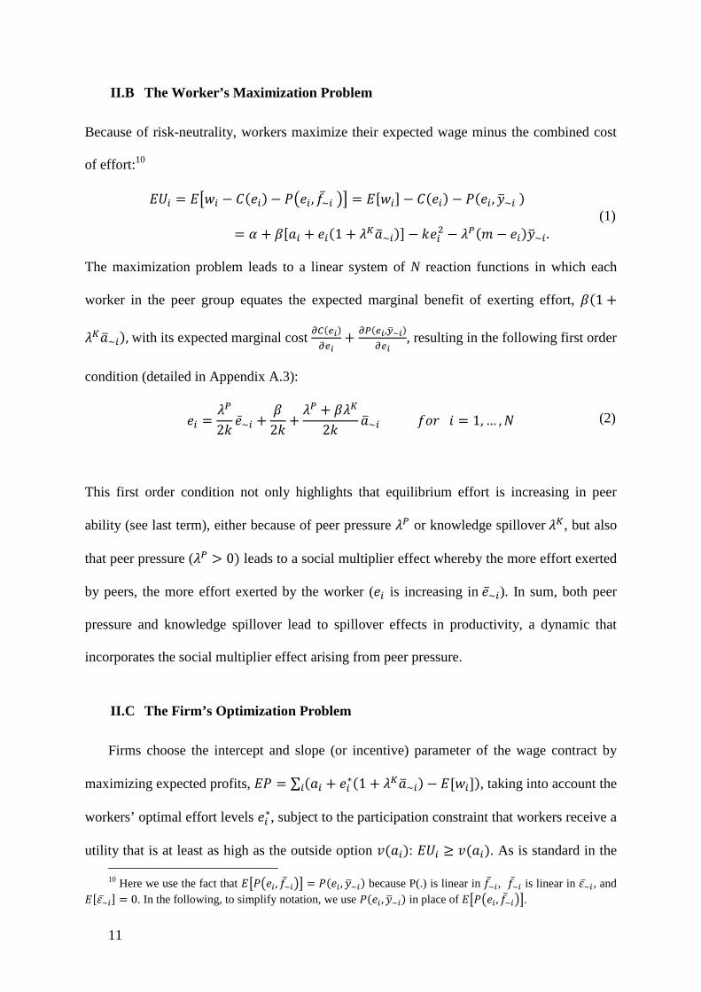
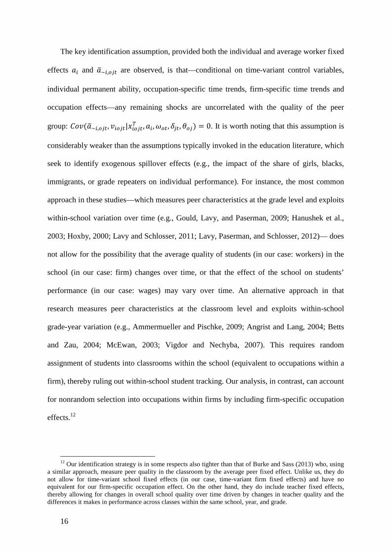
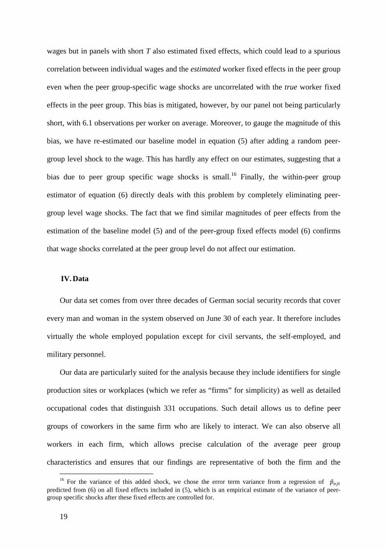
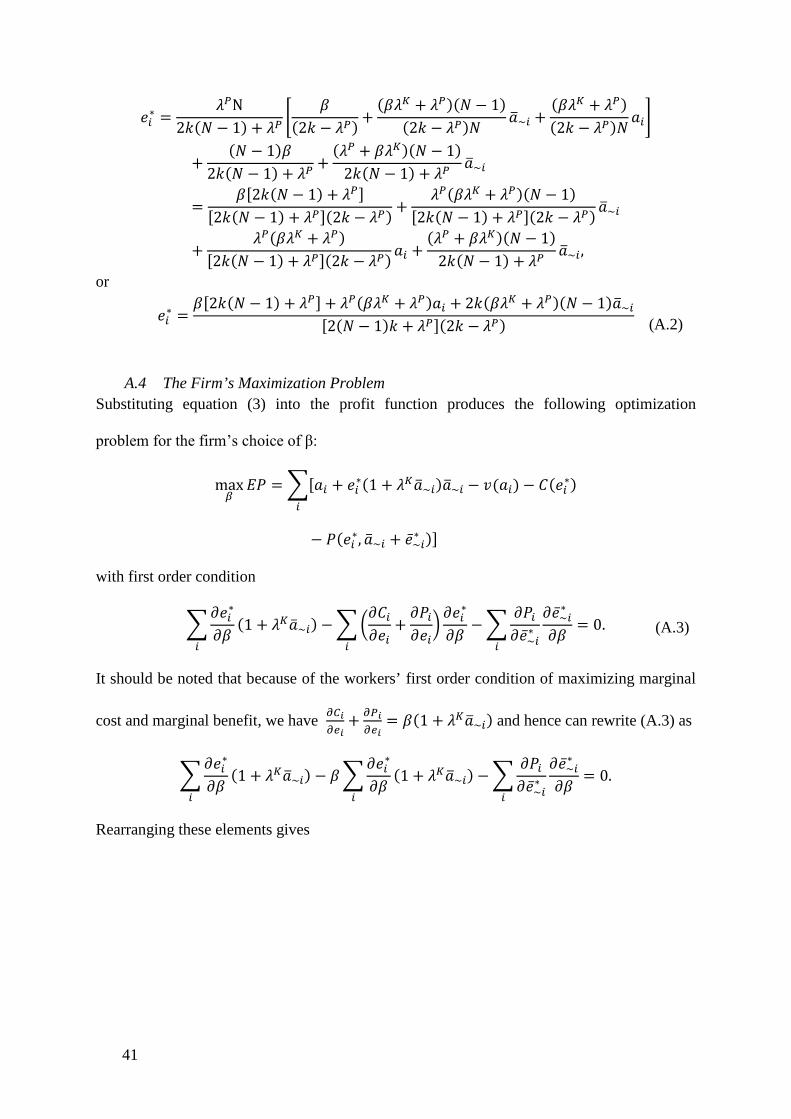
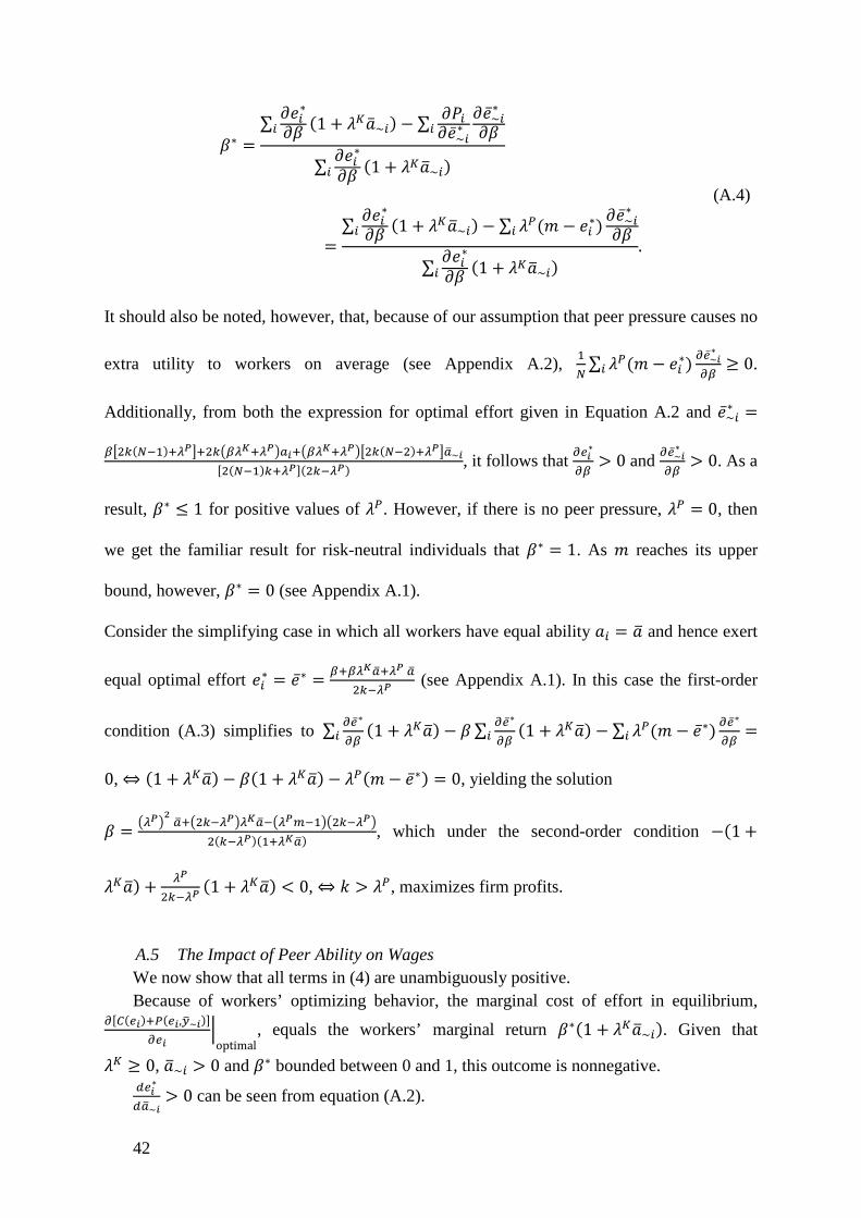
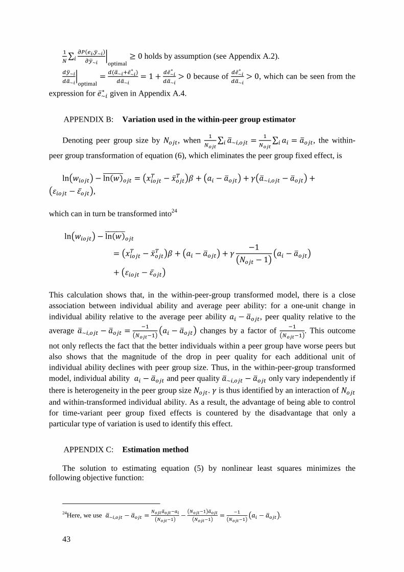
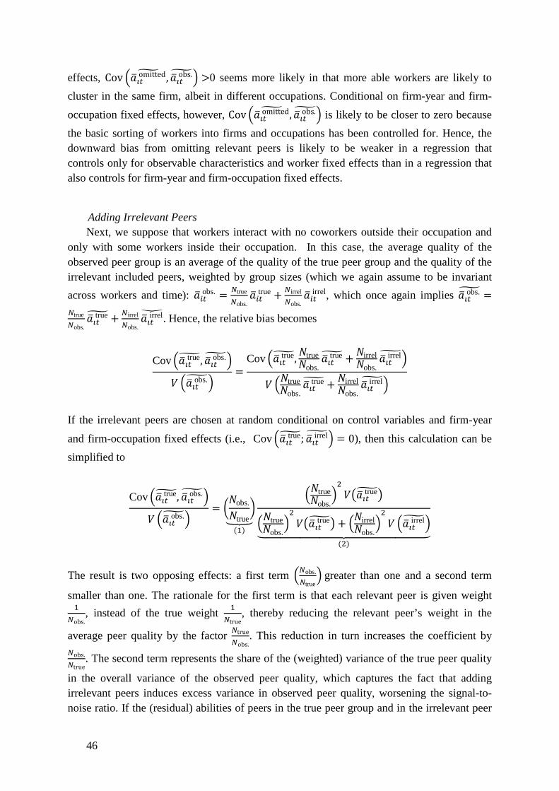
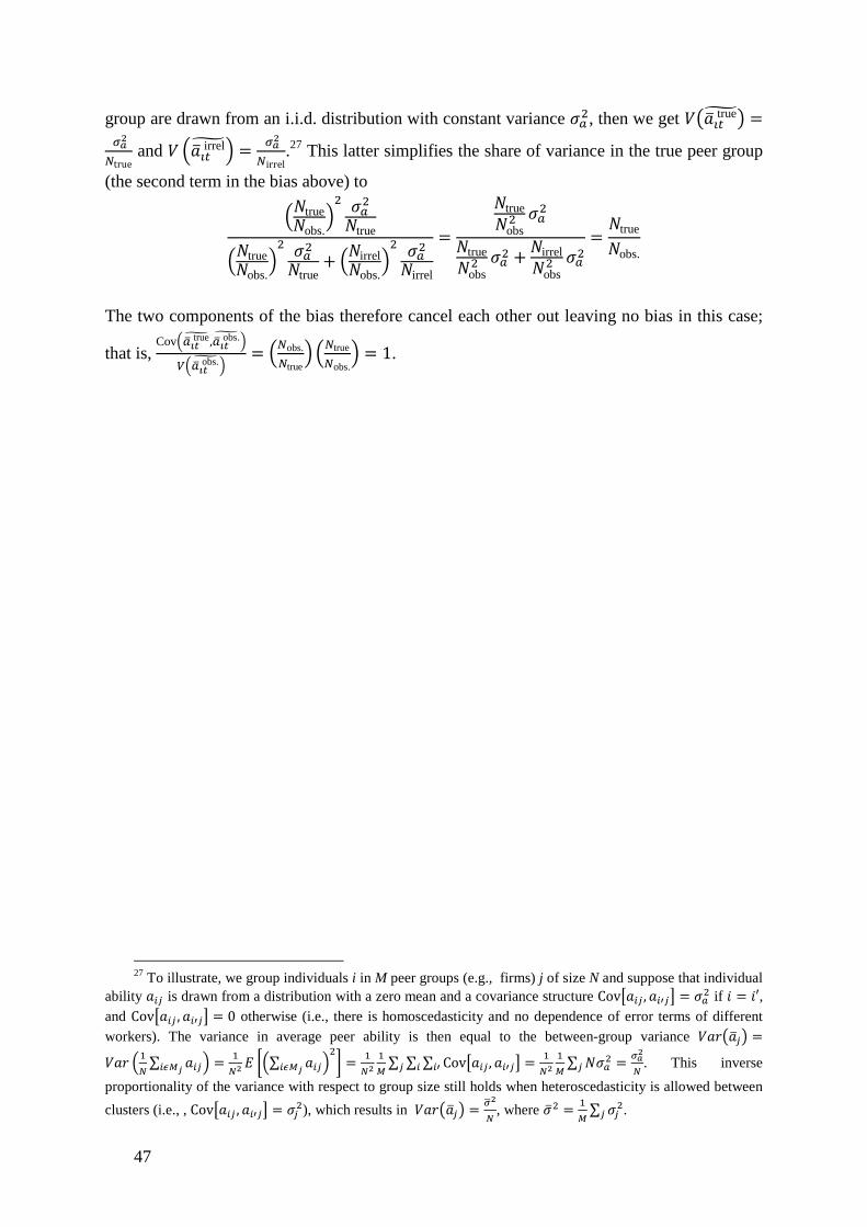
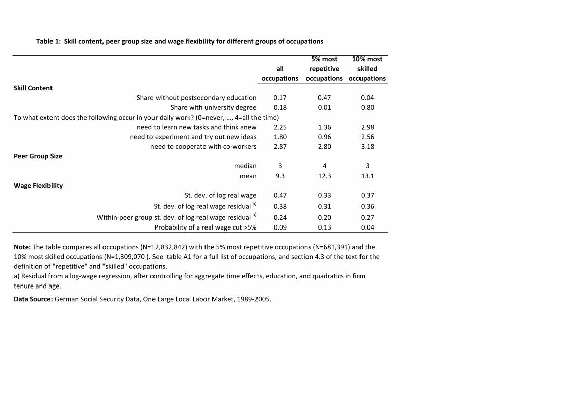
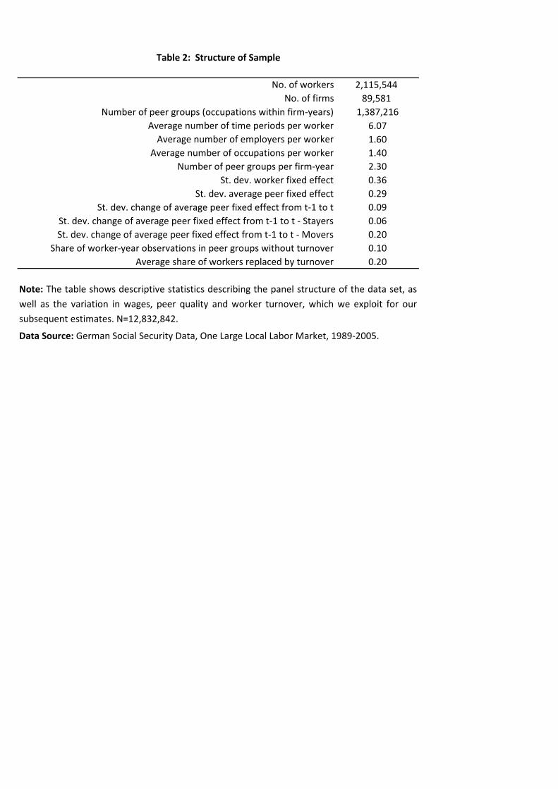
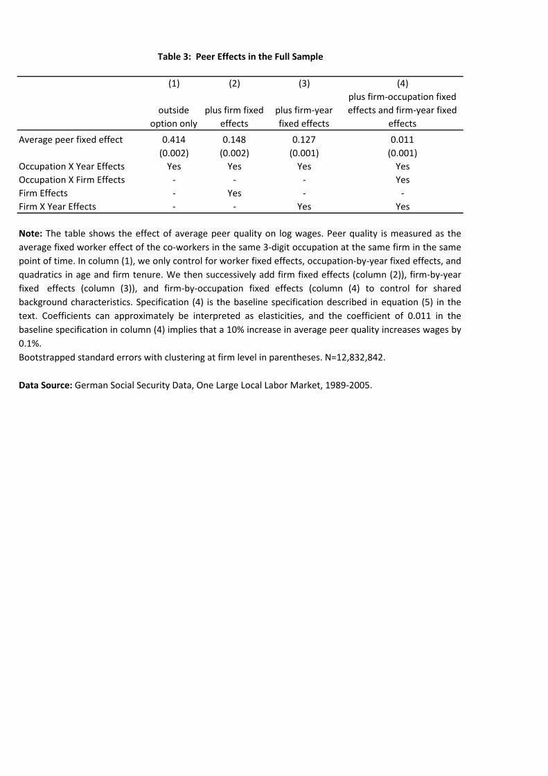
(1) (2) (3) (4)
Average peer fixed effect 0414 0148 0127 0011
(0002) (0002) (0001) (0001)
Occupation X Year Effects Yes Yes Yes Yes
Occupation X Firm Effects - - - Yes
Firm Effects - Yes - -
Firm X Year Effects - - Yes Yes
Data Source German Social Security Data One Large Local Labor Market 1989-2005
Table 3 Peer Effects in the Full Sample
Note The table shows the effect of average peer quality on log wages Peer quality is measured as the
average fixed worker effect of the co-workers in the same 3-digit occupation at the same firm in the same
point of time In column (1) we only control for worker fixed effects occupation-by-year fixed effects and
quadratics in age and firm tenure We then successively add firm fixed effects (column (2)) firm-by-year
fixed effects (column (3)) and firm-by-occupation fixed effects (column (4) to control for shared
background characteristics Specification (4) is the baseline specification described in equation (5) in the
text Coefficients can approximately be interpreted as elasticities and the coefficient of 0011 in the
baseline specification in column (4) implies that a 10 increase in average peer quality increases wages by
01
Bootstrapped standard errors with clustering at firm level in parentheses N=12832842
outside
option only
plus firm fixed
effects
plus firm-year
fixed effects
plus firm-occupation fixed
effects and firm-year fixed
effects
(1) (2) (3)
5 most repetitive
occupations
As in case studies Low learning content
Average peer fixed effect 0064 0067 0052
(00070) (00116) (00031)
Average peer fixed effect 0013 0007 0017
(00039) (00044) (00028)
Data Source German Social Security Data One Large Local Labor Market 1989-2005
Note The table shows the effect of average peer quality on log wages for different occupational
groups Peer quality is measured by the average worker fixed effect of the co-workers in the same 3-
digit occupation at the same firm in the same point of time All models implement the baseline
specification see equation (5) of the text and include occupation-by-year occupation-by-firm firm-by-
year and worker fixed effects and controls for quadratics in age and firm tenure
In panel A column (1) we show the effect for the 5 most repetitive occupations In panel A column
(2) we show the effect for agricultural helpers cashiers and data entry workers which have been used
in related case-studies on peer effects in the workplace In panel A column (3) we report the effect for
occupations characterized by standardized tasks (as the 5 most repetitive occupations) and limited
learning content (ie cashiers warehouse workers drivers removal workers cleaners agricultural
helpers and waiters) In panel B column (1) we present results for the 10 most skilled occupations as
measured by the share of workers with a college degree in that occupation In panel B column (2) we
present results for the 10 most innovative occupations defined by occupation averages of workers
responses to an index of how frequently they need to experiment with new ideas In panel B column
(3) we present results for occupations with complex tasks and a high learning content (such as doctors
lawyers scientists teachers and academics) See Table A1 for a full list of occupations in each of the
sub-samples used in this table and section 43 in the text for an explanation of the way in which the
different sub-samples were constructed
Bootstrapped standard errors with clustering at firm level in parentheses N=12832842
Table 4 Peer Effects in Sub-Samples of Occcupations
Panel A Peer Effects for Sub-Samples of Low Skilled Occupations
Panel B Peer Effects for Sub-Samples of High Skilled Occupations
High learning content10 most innovative
occupations
10 most skilled
occupations
(1) (2) (3) (4)
Within peer group
estimatorWage not imputed
Peer group defined
at 2-digit
occupational level
Varying coeff on
observables
Average peer fixed effect 0061 0086 0067 0082
(0006) (0007) (0005) (0008)
Average peer fixed effect 0016 0017 0010 0007
(0004) (0007) (0003) (0004)
Data Source German Social Security Data One Large Local Labor Market 1989-2005
Table 5 Robustness Checks
Note Note The table reports a number of robustness checks for the effect of average peer quality on log wages
Panel A shows the robustness checks for the group of the 5 most repetitive occupations as in column (1) Panel
A of Table 4 Panel B reports the robustness checks for the group of the 10 most skilled occupations as in
column (1) Panel B of Table 4
In column (1) we present the within peer group estimate see equation (6) in the text The within-estimator is
based on pre-estimated worker fixed effects from the baseline model in equation (5) in the text The remaining
columns refer to our baseline specification given by equation (5) in the text In column (2) we do not impute
censored wage observations In column (3) we define the peer group at the 2-digit occupational level instead of
the 3-digit occupational level In column (4) we allow the coefficients on the observable characteristics
(quadratics in age and firm tenure) to vary between the 5 most repetitive (or 10 most skilled) occupations and
the remaining occupations
Bootstrapped standard errors with clustering at firm level in parentheses N=12832842
Panel A 5 Most Repetitive Occupations
Panel B 10 Most Skilled Occupations
Panel A Knowledge Spillovers or Peer Pressure Age and Tenure Interactions
(1) (2)
age interaction tenure interaction
Average peer fixed effect 0089 0058
(00088) (00067)
Average peer fixed effect Age gt 35 -0039
(00110)
Average peer fixed effect Peer tenuregt=2 0007
(00092)
Panel B Knowledge Spillovers or Peer Pressure Lagged Peer Group (pre-estimated)
Average peer fixed effect t
Average peer fixed effect t-1
Average peer fixed effect
Average peer fixed effect Co-operation not
important
Average fixed effect of middle 80 peers
Average fixed effect of top 10 of peers
Average fixed effect of bottom 10 of peers
Table 6 Peer Pressure or Other Channels (5 Most Repetitive Occupations)
Panel D Distinguishing between Top vs Bottom Peers (pre-estimated)
top vs bottom peers
0072
(00032)
(00034)
Panel C Comlementarities or Peer Pressure
0081
(00078)
-0040
(00110)
cooperation interaction
inclusion of lagged peer group
0054
(00034)
-0005
(00014)
All specifications refer to our baseline specification and cotrol for quadratics in age and firm
tenure worker fixed effects occuption-by-time fixed effects firm-by-year fixed effects and
firm-by-occupation fixed effects Bootstrapped standard errors with clustering at firm level in
parentheses
Note The table provides evidence that the peer effect in wages for the 5 most repetitive
occupations are not (only) driven by knowledge spillovers or complementarities in
production In Panel A we allow the effect of average peer quality on log wages to differ
between workers below and above age 35 (column (1)) and between workers who have
been in the peer group more and less than 2 years (column (2)) In Panel B we add the
average fixed effects of the lagged peer group to equation (5) based on pre-estimated fixed
effects from the baseline model In Panel C we allow the peer effect to vary in occupations
with below- or above-median shares of workers who report that cooperation is important in
their job (column (1)) In Panel D we split the workers peers up into the middle 80 top
10 and bottom 10 according to their ability ranking This specification is again based on
pre-estimated worker fixed effects and the regression in Panel D is run on the sample for the
middle 80 of workers only
0003
(00013)
0007
Data Source German Social Security Data One Large Local Labor Market 1989-2005
Change in average peer fixed effect 0054 0047
(0008) (0008)
Average peer fixed effect 0066 0032
(0006) (0006)
men women
Average peer fixed effect 0054 0075
(0008) (0008)
Note In Panel A we investigate whether improvements an deteriorations in average
peer quality have similarly sized effects To do this we adopt an approach similar to
Mas and Moretti (2009) and regress for peer group stayers the change in log wages
on the change in peer group quality (using the pre-estimated worker fixed effects
from our baseline specification) and allow this effect to vary according to whether
peer group quality improved or deteriorated In Panel B we let the peer effect vary by
whether the focal worker is above or below the peer-group mean of ability In Panel
C we let the peer effect vary by the focal workers gender
Panel C Heterogenous Effects by Gender
Data Source German Social Security Data One Large Local Labor Market 1989-2005
Table 7 Heterogeneous Peer Effects (5 Most Repetitive Occupations)
Panel A Symmetry of Peer Effects (First Differences Peer Group Stayers Pre-
Estimated Effects)
Negative Change Positive Change
focal worker below
median
Panel B Heterogeous Effects by Relative Position within the Peer Group
focal worker above
median
5 most repetitive occupations Share Hand-picked occupations with low Share 10 most skilled occupations Share
in learning content in in Unskilled laborer helper (no further specification) 1512 Salespersons 240 Electrical engineers 243Packagers goods receivers despatchers 1158 Motor vehicle drivers 194 Mechanical motor engineers 131Metal workers (no further specification) 1066 Store and warehouse workers 109 Management consultants organisors 103Postal deliverers 758 Household cleaners 89 Other engineers 76Assemblers (no further specification) 547 Waiters stewards 80 Architects civil engineers 73Street cleaners refuse disposers 470 Unskilled laborer helper (no further specification) 59 Physicians 52Assemblers of electrical parts or appliances 468 Packagers goods receivers despatchers 45 Economic and social scientists statisticians 47Cashiers 400 Gardeners garden workers 37 Scientists 38Railway controllers and conductors 396 Goods examiners sorters nec 33 Ministers of religion 32Laundry workers pressers 369 Street cleaners refuse disposers 18 Other manufacturing engineers 29Machinery or container cleaners and related occupations 287 Cashiers 16 Senior government officials 29Railway engine drivers 280 Glass buildings cleaners 15 Physicists physics engineers mathematicians 25Milk and fat processing operatives 262 Laundry workers pressers 14 Technical vocational factory instructors 20Vehicle cleaners servicers 257 Transportation equipment drivers 14 Legal representatives advisors 19Clothing sewers 202 Vehicle cleaners servicers 10 Primary secondary (basic) special school teachers 17Wood preparers 196 Earthmoving plant drivers 08 Chemists chemical engineers 15Metal grinders 192 Construction machine attendants 07 University teachers lecturers at higher technical schools and academies 13Ceramics workers 120 Crane drivers 04 Gymnasium teachers 13Brick or concrete block makers 106 Stowers furniture packers 03 Pharmacists 08Tobacco goods makers 097 Agricutlural helpers 03 Academics Researchers in the Humanities 08Sheet metal pressers drawers stampers 086 Garden architects garden managers 04Solderers 086 Survey engineers 03Agricutlural helpers 075 Veterinary surgeons 01Model or form carpenters 068 Mining metallurgy foundry engineers 01Sewers 066 Dentists 01Meat and sausage makers 061Stoneware and earthenware makers 049
Enamellers zinc platers and other metal surface finishers 042
Leather clothing makers and other leather processing operatives 033 10 most innovative Share Hand-picked occupations with high Share
Metal moulders (non-cutting deformation) 027 occupations in learning content in Rubber makers and processors 027 Data processing specialists 387 Electrical engineers 206Other wood and sports equipment makers 024 Electrical engineers 247 Entrepreneurs managing directors divisional managers 181Earth gravel sand quarriers 022 Mechanical motor engineers 133 Mechanical motor engineers 111Machined goods makers 020 Architects civil engineers 75 Management consultants organisors 87Moulders coremakers 019 Scientists 38 Other engineers 65Vulcanisers 018 Other manufacturing engineers 29 Architects civil engineers 62Textile finishers 016 Physicists physics engineers mathematicians 25 Chartered accountants tax advisers 55Footwear makers 015 Chemists chemical engineers 15 Physicians 44Other textile processing operatives 015 University teachers lecturers at higher technical schools and academies13 Economic and social scientists statisticians 40Ready-meal fruit and vegetable preservers and preparers 013 Musicians 09 Scientists 32Weavers 013 Interior exhibition designers window dressers 08 Other manufacturing engineers 25Spinners fibre preparers 012 Packaging makers 05 Senior government officials 24Textile dyers 009 Garden architects garden managers 04 Physicists physics engineers mathematicians 21Planers 007 Brokers property managers 03 Legal representatives advisors 16Spoolers twisters ropemakers 005 Survey engineers 03 Chemists chemical engineers 13Post masters 005 Scenery sign painters 02 Humanities specialists 07Radio operators 004 Veterinary surgeons 02 Association leaders officials 06Hat and cap makers 004 Mining metallurgy foundry engineers 01 Survey engineers 03Ship deckhand 004 Forestry managers foresters hunters 01 Veterinary surgeons 01Cartwrights wheelwrights coopers 003 Coachmen 00 Mining metallurgy foundry engineers 01Rollers 003 Dentists 01Wood moulders and related occupations 002Fine leather goods makers 002Fish processing operatives 001Metal drawers 001
Jewel preparers 001
Table A1 List of Occupations for different Sub-Samples
(1) (2)
(4)
Note The table presents the lists of occupations in for the different sub-samples of occupations used in table 4
Data Source German Social Security Data One Large Local Labor Market 1989-2005 N=12832842
(3)
(5)
Figure 1 Variablity of Wages Across and Within Peer Groups
Note The figure compares all occupations (N=12832842) the 5 most repetitive
occupations (N=681391) and the 10 most skilled occupations (N=1309070 ) in
terms of the variability of wages
Residualized wages are computed from a log-wage regression controlling for
aggregate time effects education and quadratics in firm tenure and age
Data Source German Social Security Data One Large Local Labor Market 1989-2005
000
005
010
015
020
025
030
035
040
045
050
All occupations 5 most repetitiveoccupations
10 most skilledoccupations
St dev oflog real wage
St dev of residualizedlog real wages
Within-peer group st dev ofresidualized log real wages
Figure 2 Variation of the Change in Peer Quality
Note The figure plots a kernel density estimate of the change in the average peer
fixed effect (FE) separately for peer group stayers and peer group movers Peer
group quality varies more strongly for movers For stayers there is a mass point at
zero corresponding to stayers in peer groups that had no turnover The figure is
trimmed at the 5 and 95 percentile of the distribution
Data Source German Social Security Data One Large Local Labor Market 1989-
2005
050
100
150
Densi
ty
-1 -05 0 05 1x
Peer FE change stayers
Peer FE change movers
- titel7617pdf
-
- University College London
- and CReAM
- University College London
- CReAM IAB and IZA
- Discussion Paper No 7617
- September 2013
- ABSTRACT
-
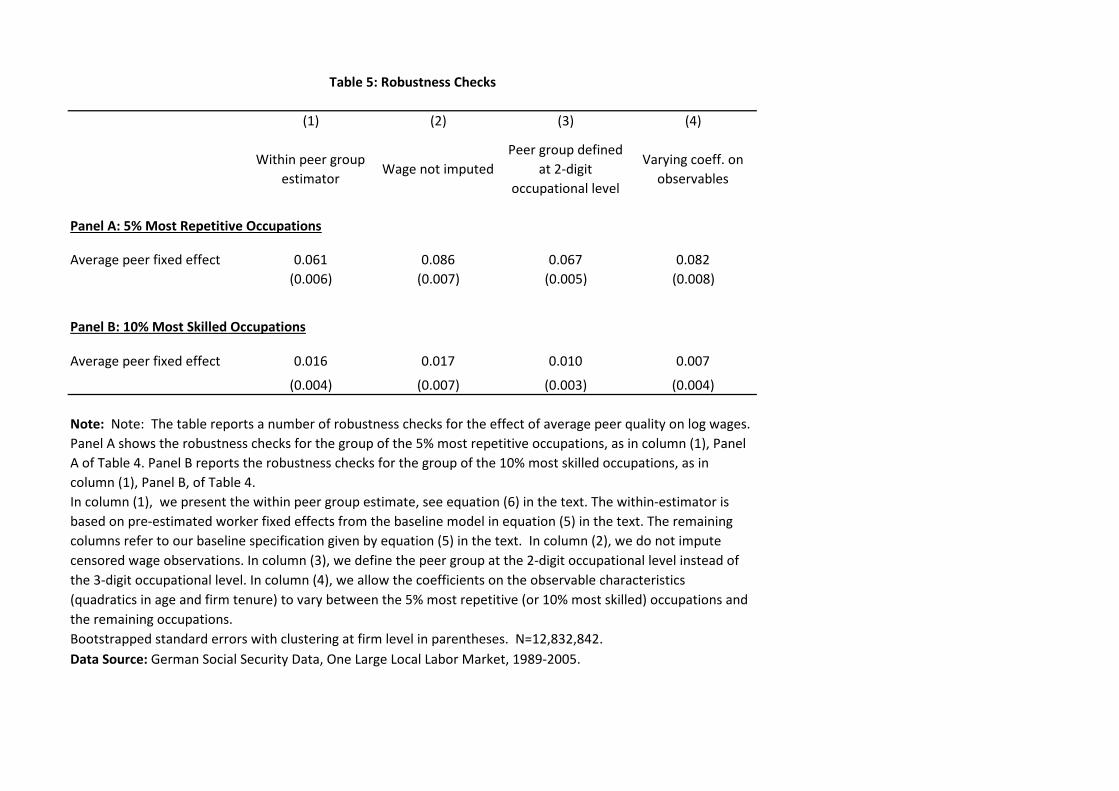
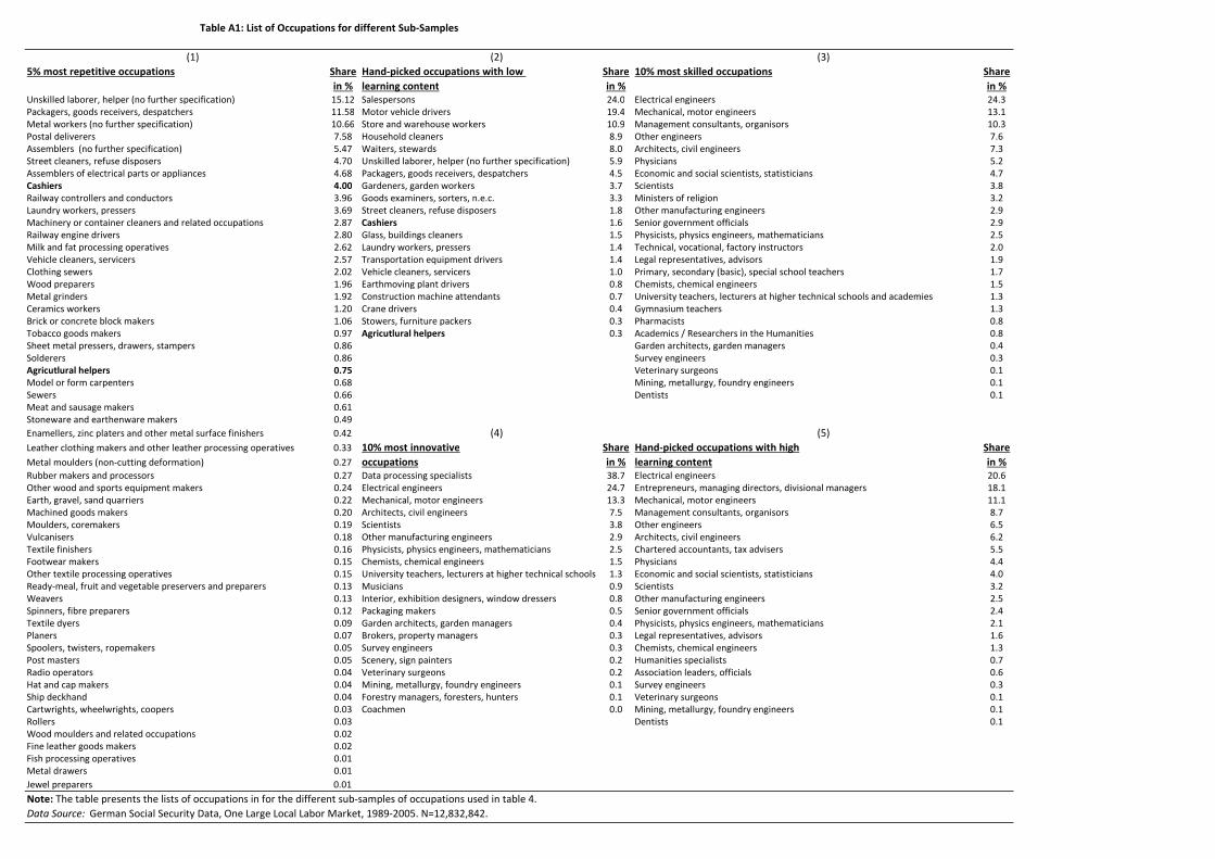