Peaceman’s Numerical Productivity Index for Non-Linear ...

Peaceman’s Numerical Productivity Index for Non-Linear Flows in Porous Media

by

Dahwei Chang, Ph.D.

A Thesis

In

MATHEMATICS

Submitted to the Graduate Faculty of Texas Tech University in

Partial Fulfillment of the Requirements for

the Degree of

MASTER OF SCIENCE

IN

MATHEMATICS

Approved

Dr. Eugenio Aulisa Chairperson of the Committee

Dr. Magdalena Toda

Dr. Victorie Howle

Fred Hartmeister Dean of the Graduate School

August, 2009

Texas Tech University, Dahwei Chang, August 2009

ii

ACKNOWLEDGMENTS

It is with Dr. Aulisa’s guidance that I am able to finish this work. At my age, I

thought I have learned to have good patience. He definitely has more patience than I

do. This research is a small portion of his master plan to find solutions for non-linear

flows in porous media. I am glad to have participated in it.

My committee members: Dr. Toda and Dr. Howle are very nice to me. They

are very patient and knowledgeable. Thank you very much!


iii

TABLE OF CONTENTS

ACKNOWLEDGMENTS ...…………………………….………………ii

ABSTRACT ……………………………………………………………..v

LIST OF TABLES ……………………………………………………....vi

LIST OF FIGURES ..…………………………………………………...vii

CHAPTER

I. INTRODUCTION ……………………………..…………………..1

II. THEORY ……………………………………….............................3

2.1 Darcy’’s Law ……………………………………..3

2.2 Formulation of the Problem ………………………4

2.3 Set up the Initial Boundary Value Problem ……...7

2.4 Initial Boundary Value Problem ……………..…..9

2.5 Auxiliary Boundary Value Problem …………….10

2.6 Summary of the PSS Regime ………………..….12

2.7 Geometry of the Simulation ……………………..13

III. PEACEMAN NUMERICAL PRODUCTIVITY INDEX FOR

DARCY (LINEAR) FLOWS ……………………….............................14


iv

IV. PEACEMAN BUMERICAL PRODUCTIVITY INDEX FOR

NON-DARCY (NON-LINEAR) FLOWS .….............................17

V. RELATIONSHIP BETWEEN ACTUAL WELL AND THE WELL

BLOCK …………………………………………………………..19

VI. DATA AND RESULTS …………………………………….........21

6.1 The Block Invariant c …………..………………..21

6.2 Application of the Block Invariant c.……………..22

6.3 Radii ro and r1 ………………………………………24

6.4 The Degrees of Freedom ………………………….25

VII. CONCLUSION ….………………………………………………. 26

BIBLIBIOGRAPHY ……………………………………………......... 27


v

ABSTRACT

From Darcy’s law to the Darcy-Forchheimer equation, there has been a lot of

effort put into finding solutions for flows in porous media. Peaceman used a system

of well blocks to replace the well bore in finding numerical solutions for linear flows.

Our work uses a single well block to find the pressure distribution throughout the well

for non-linear flows. In the process we found a block invariant which can be used to

build the pressure distribution formula. From it, we can find the productivity index,

one of the important factors in petroleum engineering.

Theoretical derivation and numerical data are also presented in this report.


vi

LIST OF TABLES

6.1 Values of Block Invariant c for a Rectangular Reservoir ……………21 6.2 Values of Block Invariant c for a Circular Reservoir ……..…………21 6.3 Comparison of PI between Actual Well and Different Well Block Sizes for a Rectangular Reservoir ..……………………....………….22 6.4 Comparison of PI between Actual Well and Different Well Block Sizes for a Circular Reservoir ..……..…………………....………….22 6.5 Comparison of Pressure at the Well Bore between Actual Well and Different Well Block Sizes for a Rectangular Reservoir ....…………23 6.6 Comparison of Pressure at the Well Bore between Actual Well and Different Well Block Sizes for a Circular Reservoir ………………..23 6.7 Ratio of Radius ro/ Well Block Size for a Rectangular Reservoir…..24 6.8 Ratio of Radius ro/ Well Block Size for a Circular Reservoir…….....24 6.9 Degrees of Freedom …………………………………………………25


vii

LIST OF FIGURES

2.1 Linear Flow ………………………………………………………….3 2.2 Relationship between Total Discharge and Pressure Drawdown for Darcy and non-Darcy Flows …………………………………………6 2.3 Geometry of the Reservoir and the Well Bore ………………………7 2.4 Production Rate Decreases in Time …………………………………10 2.5 Well Pressure Distribution in Time ………………………………….12 2.6 Reservoir and a Well Block ………………………………………….13 2.7 Reservoir and an Actual Well ………………………………………..13 5.1 Pressure in a Well Block …………………………………….………19 5.2 Pressure in an Actual Well …………………………………………...19 5.3 Pressure Distribution …………………………………………………20


1

CHAPTER I

INTRODUCTION

There have been numerous studies on fluid filtration in porous media because

of its wide applications. One of its major applications is on flows in oil reservoirs. In

1856, Darcy 1 proposed a linear differential equation between the pressure drop and

the production rate. Later Forchheimer (1901)2 introduced a nonlinear term for high

velocity flows. Accurate numerical solutions for this Darcy-Forchheimer equation

experience difficulty in finding the pressure near the well bore due to the drastic

change in pressure. This is generally accomplished by using high resolution meshes

around the wellbore.

In an alternative approach, numerical solutions have been found by replacing

the wellbore with a grid block that is generally larger than the wellbore size. By using

the well-block finite difference numerical solution, Peaceman (1978)3 found a semi-

analytical formula for reconstructing the real pressure distribution in the wellbore

proximity and for evaluating the well productivity index for the linear Darcy case.

Aulisa and others (2007)4 introduced a generalized non-linear equation which

relates the velocity vector field of filtration to the gradient of pressure in a non-linear

way. The system formed by the latter equation, the continuity equation, the equation

of state for slightly compressible fluids and the appropriate initial and boundary

conditions defines an initial boundary value problem for the pressure only. Further

analysis showed the existence of an auxiliary boundary value problem whose solution

could be used to build a “time-invariant” solution of the initial boundary value

problem.

In this work, starting from these results, we extend Peaceman’s work to non-

linear flows by using well block finite element solutions. We show that for any well

block size there exists an invariant coefficient that allows us to reconstruct accurately


2

the actual pressure profile, even for high non-linearity. All numerical simulations

have been done by using COMSOL Multiphysics.


3

CHAPTER II

THEORY

2.1 Darcy’s Law

Darcy’s law states that the discharge rate Q is proportional to the pressure drop

over a given distance and is defined in Eq. 2.1 (see figure 1). The negative sign is

needed because fluids flow from high pressure to low pressure. Dividing both sides of

Eq. 2.1 by the area, A, and we got Eq. 2.2 which defines the Darcy flux, q.

Figure 1.1 View from my window

L) P(P A -

Q ab

µκ −= (2.1)

µκ P -

q∇= (2.2)

The pore velocity, v, is defined by the ratio of Darcy flux and the porosity of

the fluid, φ. It shows the higher the porosity, the higher the flux.

ϕq

v =→

(2.3)

Units: Q: total discharge, m3/s κ: permeability, m2 A: cross section area, m2 P: pressure, Newton/ m2 = kg/(m.s2) Q: Darcy flux, m/s L: distance, m

b A a

L Q


4

v: velocity, m/s φ: fraction µ: fluid viscosity, kg/(m.s)

If we substitute q from Eq. 2.2 into Eq. 2.3 and drop φ, we get

P v ∇=−→

κµ

(2.4)

For a fixed pressure difference, the higher the viscosity, the slower the

velocity; the higher the permeability, the higher the fluid velocity.

2.2 Formulation of the Problem

Fluid flows, which deviate from Darcy’s law, are typically observed in high-

rate well production. In non-Darcy flow, the fluid converging to the well bore reaches

velocities exceeding the lamina Reynolds number, resulting in a turbulent regime.

There are different approaches for modeling non-Darcy phenomena. It seems that the

most appropriate is derived from the general Brinkman-Forchheimer equation. The

derivation of this equation by Aulisa et al. (2009)5 is as follows.

Let ∇ and ∆ denote the gradient and the Laplace operator. The time dependent

Brinkman-Forchheimer equation describing the velocity vector field →v and the

pressure P in porous media can be written in the form

a

v c - v v || v || v - P

t

µρ µ βκ

→→ → → ∂ ∆ + + = ∇

∂

, (2.5)

with 1/2

F

κϕρβ = ,

Here ca is the acceleration coefficient, F is the Forchheimer coefficient, φ is the

porosity, κ is the permeability, µ is the viscosity and ρ is the density of the fluid.

The continuity equation can be written in the form


5

0 )v( =⋅∇+∂∂ →

ρρt

(2.6)

In order to solve this system of equations, we assume that the first two terms in

Eq. 2.5 can be neglected. We also assume the fluid is slightly compressible and

satisfies the state equation

ργρ -1' = ( )e )P - (P 0

o-1γρρ = , (2.7)

where the γ – constant characterizes the compressibility of the fluid.

Then the three governing equations for non-Darcy flows becomes

P, v - )v( - t

P '' ∇⋅⋅∇=∂∂ →→

ρρρ (2.8)

0 v ||v|| - v - P =∇−→→→

βκµ

, (2.9)

ργρ -1' = , (2.10)

For slightly compressible liquids coefficient -1 γ is of the order of 10-8,

therefore, following the engineering tradition, the second term in Eq. 2.8, P v ' ∇⋅→

ρ

(small compare to the first term) will be neglected. Finally these three equations can

be rewritten as

, )v( - t

P '

→⋅∇=

∂∂ ρρ (2.11)

0 v ||v|| - v - P =∇−→→→

βκµ

. (2.12)

Equation 11 is referred as the continuity equation. Equation 2.12 is referred as

the Darcy-Forchheimer equation and Eq. 2.10 as the equation of state for slightly

compressible liquids. Equation 2.11 and 2.12 describe flows in porous media.


6

Figure 2.2 shows the relationship between total discharge and pressure

drawdown for Darcy and non-Darcy flows.

Darcy flow: P v ∇=−→

κµ

(2.4)

Non-Darcy flow: 0 v ||v|| - v - P =∇−→→→

βκµ

(2.12)

Figure 2.2 Relationship between Total Discharge and Pressure Drawdown for Darcy and non-Darcy Flows

The velocity vector field t)(x, v→

as a dependent variable can be uniquely

represented as a function of the pressure gradient. Let us assume the following

approximation of the Darcy-Forchheimer equation (Eq. 2.12)

v - (|| P||) Pf→

= ∇ ∇ . (2.13)

The length of the vector ||v||→

is defined correspondingly as


7

|| v || (|| P||) || P||f→

= ∇ ∇ . (2.14)

It can be proved that →v defined in Eq. 2.13 solves Eq. 2.12, where f is defined

by the following,

2

2f

4 || P|| α α β=

+ + ∇ 2.3 Set up the Initial Boundary Value Problem

In our model the exterior boundary of the reservoir is considered impermeable.

The boundary condition on the well, the condition of non-flux on the exterior

boundary of the reservoir, and the prescribed initial pressure distribution together form

the initial boundary value problem (IBVP) for system Eq. 2.7 – 2.9. Figure 2.3 shows

the geometry of the reservoir and the well bore.

Let U ⊂ Rn, n = 1, 2, or 3 be the reservoir domain bounded by the exterior

impermeable boundary, and the well interface

U

W

ΓU

Γw

Figure 2.3 Geometry of the Reservoir and the Well Bore


8

compact. and with, U UWUWU,W ΓΓ∅=Γ∩ΓΓ∪Γ=∂

The part ΓU is associated with the exterior boundary of the reservoir U, and the

part ΓW is associated with the boundary of the well. Let P(x, to) = Po(x) be the given

initial pressure distribution in the reservoir.

We define the following notation. If P is a function defined on Ū, then let UP

and WP denote the average of P on U and ΓW respectively, defined by

W

W

1P ( ) = P(x, t) d s

| W| xtΓ∫ - average value of the pressure on the well;

U

U

1P ( ) = P(x, t) d x

| U|t

Γ∫ - average value of the pressure in the reservoir;

x = Rn - spatial independent variable, n = 1, 2, 3;

|W| = mesn-1 U - area of the well;

|U| = mesn U - volume of the reservoir. Definition (Diffusive Capacity)

Let the pressure function P(x, t) and the vector velocity v→

(x, t) form the

solution of system (Eq. 2.7 - 2.9) in the bound domain U, with boundary condition

Uv (x, t) n | = 0.→ →

Γ⋅ Assume for any t > 0, P(x, t) to be such that UP (t) > WP (t).

The diffusive capacity of ΓW with respect to ΓU corresponding to the solution P(x, t)

and v→

(x, t) is the ratio

W

x

U W

v(x, t) n d s

J (P, v, t) = .P (t) - P (t)

→ →

→Γ

⋅∫ (2.15)

Here n→

is the external normal on the piecewise smooth surface ΓW.


9

Definition (PSS regime)

Let the well production rate Q be time independent: W

xv(x, t) n d s = Q.→ →

Γ

⋅∫

We will call the system a “pseudo-steady state regime” (PSS), if the

corresponding pressure drawdown (difference between the average of the pressure on

the well surface and the average of the pressure in the reservoir) is constant. For the

PSS regime the diffusive capacity /PI is time invariant.

The diffusive capacity is not unique and depends not only on the boundary

condition on ΓW but also on the class of admissible functions, on which the functional

J (P, v→

, t) is defined. The main reason why diffusive capacity is introduced in this

way is to reflect the major engineering idea behind the Productivity Index. The other

reason is because of its generality.

2.4 Initial Boundary Value Problem

Let the domain U, its boundaries, and the initial pressure function have the

same meaning as in section 2-4. Assume that the well is operating under the condition

of time independent constant production rate Q; the initial reservoir pressure is known.

Then under assumptions in the previous section the initial boundary value problem

(IBVP) modeling the filtration process can be formulated as follows

' P = - ( v),

tρ ρ

→∂ ∇ ⋅∂

(2.16)

P - v - || v || v = 0,µ βκ

→ → →− ∇ (2.17)

W

v n d s = Q ,→ →

Γ

⋅∫ (2.18)


10

Uv n | = 0 ,→ →

Γ⋅ (2.19)

0P(x, 0) = P (x) . (2.20)

In addition, by using assumption that β is constant and the fluid is

incompressible, Eq. 2.16 – 2.20 reduces to

1 P = ( (f(|| P||)) P) ,

tγ − ∂ ∇ ⋅ ∇ ∇

∂ (2.21)

W

Pf (|| P||) d s = - Q ,

n→

Γ

∂∇∂

∫ (2.22)

U

P | = 0 ,

nΓ→

∂

∂ (2.23)

0P(x, 0) = P (x) . (2.24)

The IBVP (Eq. 2.21 – 2.24) is ill-posed: it has an infinite number of solutions.

Remember that the Productivity Index is modeled as an integral characteristic of the

solution, hence, the lack of uniqueness in the definition. Later we will restrict the

solution by introducing a class of functions for which it is unique up to an additive

constant.

2.5 Auxiliary Boundary Value Problem

In Eq. 2.21, pressure P is a function of time and position. In a real well, once

the well starts producing, the production rate in the well decreases and soon settles

down to a constant value as in figure 2.4. The pressure distribution throughout the

reservoir is also settles down to a constant distribution.

Q


11

Figure 2.4 Production Rate Decreases in Time

We are interested in finding this pressure distribution. Therefore, we suggest

the following expression for the pressure. In this expression, the factor of time and

position are separated.

B. t |U|

Q - (x)W t)(x, P += γ (2.25)

If we substitute Eq. 2.25 into Eq. 2.21 – 2.24, then the IBVP becomes

W), ||)W(|| f ( A - |U|

Q ∇∇⋅∇==− (2.26)

0, |W

W=Γ (2.27)

W

| = 0 ,n

UΓ→∂

∂ (2.28)

The divergence theorem implies

W

Wf (|| W||) d s = - Q .

n→

Γ

∂∇∂

∫ (2.29)

Time


12

The equation system Eq. 2.26 – 2.29 is the auxiliary boundary value problem.

Eq. 2.27 describes a Dirichlet boundary condition for W. Eq. 2.28 describes the

Neumann boundary condition for W, i.e. no flux out of the reservoir. The solution of

this BVP exists and is unique in an appropriate functional space. Our simulation is set

to solve these equations. We assume the steady state production rate Q and define A =

Q/|U|, A is a constant. We also assume that the boundary U∂ is smooth. Figure 2.5

shows the relationship between P(x, t) and W(x).

Figure 2.5 Well Pressure Distribution in Time 2.6 Summary of PSS regime

Let assumptions in section 2-2 hold. If the initial function P0(x, 0) = W(x) in

Eq. 2.25 is a solution of auxiliary BVP (Eq. 2.26 – 2.29), then the diffusive capacity is

steady state invariant over the solution of IBVP (Eq. 2.21 – 2.24), and can be

computed by using the formula

B

P(x,t)

t

x

W(x)


13

WWU U

Q QJ (P, v, t) = J (Q, t) = = = J (Q) ,

1 1 1P dx - P dx W(x) dx

|U| | | |U|

→

ΓΓ∫ ∫ ∫

Although P is a function of time (so is its average), the pressure difference is

independent of time. Therefore J (Q) is time invariant and depends on α, β, Q, and on

the geometry of the domain U.

2.7 Geometry of the Simulation

In our simulation, as in figure 2.6, we follow Peaceman’s idea in which a well

block is used to replace the well bore and set no boundary conditions on the block.

Because there is no boundary condition on the block, less number of elements are

needed when equation system is solved based on the finite element method. Hence,

less number of mesh points and degrees of freedom are needed. This advantage may

become useful when the solution is extended to include time factor or for compressible

fluid.

Figure 2.6 Reservoir and a Well Block Figure 2.7 Reservoir and an Actual Well

U2

U1


14

For our geometry, the auxiliary BVP of Eq. 2.26 – 2.29 are transformed into Eq. 2.30 – 2.33.

W) ||)W(|| f ( A - |U|

Q ∇∇⋅∇==− u) ||)u(|| f (

|U|Q

1

∇∇⋅∇=− on U1 (2.30)

0, |WW

=Γ u) ||)u(|| f ( |U|

Q

2

∇∇⋅∇=− on U2 (2.31)

W

| = 0 ,n

UΓ→∂

∂ 0

n

W |U

=Γ∂

∂→ (2.32)

W

Wf (|| W||) d s = - Q .

n→

Γ

∂∇∂

∫ Q - s d n

u ||)u(|| f

2

=∂

∂∇∫Γ

→ (2.33)


15

CHAPTER III

PEACEMAN NUMERICAL PRODUCTIVITY INDEX FOR DARCY

(LINEAR) FLOWS

One of the important factors in petroleum engineering is the productivity index

(PI) which is defined by Darcy in the following equation.

)) P(r(P 2q

PIwaverage −

=π

α,

where q is the production rate is defined as the specific discharge per unit

cross-sectional area normal to the direction of the flow,κµα = , µ is viscosity and κ is

the permeability of the fluid. Paverage is the average pressure of the reservoir, and P(rw)

is the pressure at the well bore.

In extrapolating the value of P(rw), Peaceman replaced the well bore with a

system of well blocks. In our work, the well bore is replaced by a single well block.

Darcy’s law also states that the filtration velocity into the well bore is

proportional to the pressure difference between the well bore and the reservoir, i.e.

P - v ∇=→

α In the radial case, this equation becomes

r d

Pd - (r) v =α

In the radial case, the relationship between the this velocity and its production

rate is described as

r 2

Q - v(r)

π= (3.1)

If we combine these two equations and integrate over the radius of the well

block, we obtain


16

∫∫ =

P

P

r

r oo

Pd r d r 2

Q-

πα

and

oo r

r ln

2Q

) P(r P(r)π

α+= (3.2)

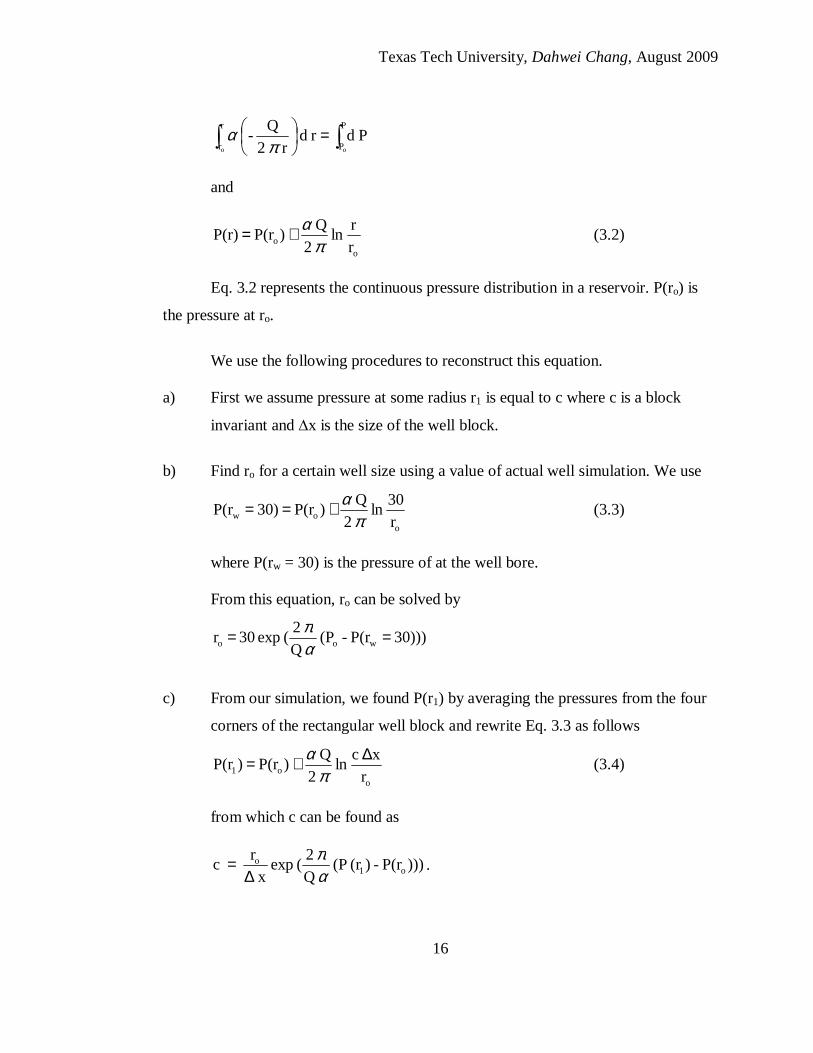
Eq. 3.2 represents the continuous pressure distribution in a reservoir. P(ro) is

the pressure at ro.

We use the following procedures to reconstruct this equation.

a) First we assume pressure at some radius r1 is equal to c where c is a block

invariant and ∆x is the size of the well block.

b) Find ro for a certain well size using a value of actual well simulation. We use

oow r

30 ln

2Q

) P(r 30)P(rπ

α+== (3.3)

where P(rw = 30) is the pressure of at the well bore. From this equation, ro can be solved by

30))) P(r- (P Q 2

( exp 30 r woo ==απ

c) From our simulation, we found P(r1) by averaging the pressures from the four

corners of the rectangular well block and rewrite Eq. 3.3 as follows

oo1 r

x c ln

2

Q ) P(r )P(r

∆+=π

α (3.4)

from which c can be found as

))) P(r- )(r (P Q

2( exp

x

r c o1

o

απ

∆= .


17

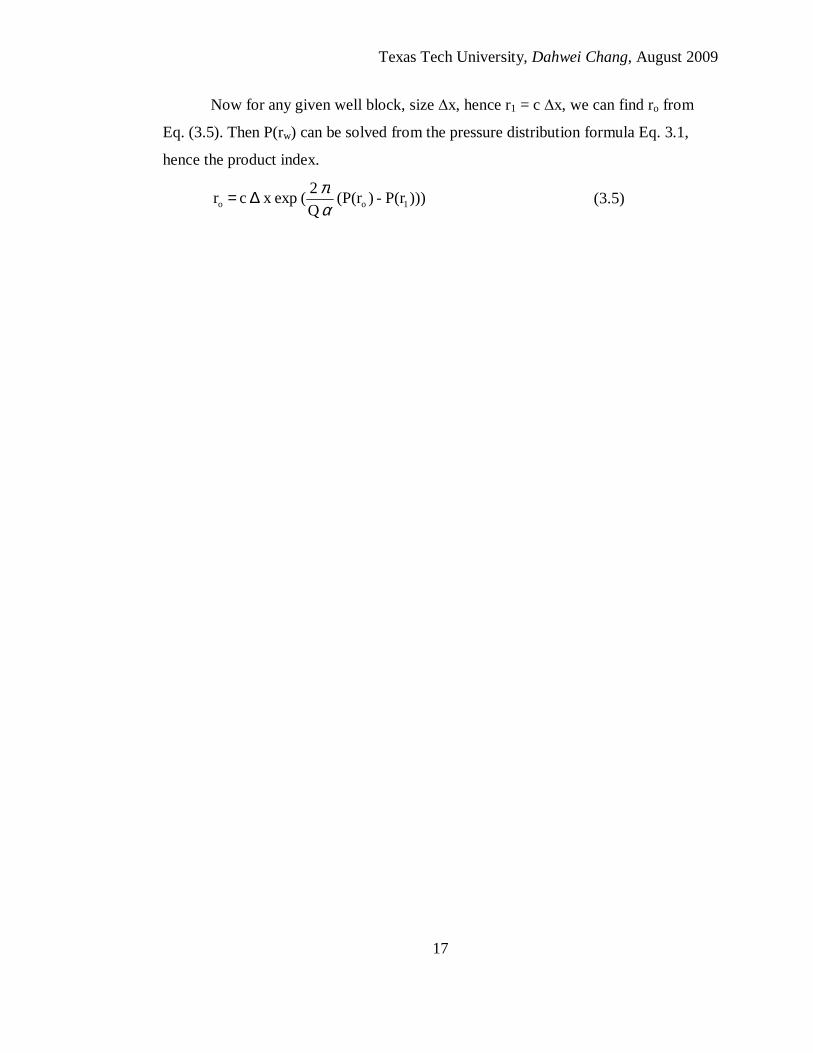
Now for any given well block, size ∆x, hence r1 = c ∆x, we can find ro from

Eq. (3.5). Then P(rw) can be solved from the pressure distribution formula Eq. 3.1,

hence the product index.

))) P(r- )(P(r Q

2( expx c r 1oo α

π∆= (3.5)


18

CHAPTER IV

PEACEMAN NUMERICAL PRODUCTIVITY INDEX FOR NON-

DARCY (NON-LINEAR) FLOWS

In the real world, flows in the porous medium are not ideally linear. Many

have added nonlinear terms to the Darcy equation. One of them is Darcy-Forchheimer

equation in which one nonlinear term that is proportional to the square of the velocity,

→v vβ , is added to the Darcy’s equation. Here β is the Forchheimer factor and is

proportional to the density of the fluid.

Darcy-Forchheimer equation

P - v ∇=+→→vv αβ (4.1)

In the radial case, this equation becomes

dr

dP - v v2 =+ αβ (4.2)

If we combine Eq. 3.1 and 4.2, integrate over the radius, we have

∫∫ =

+P

P

r

r 22

2

oo

Pd r d r 2

Q- r d

r 4Q

π

απ

β

++=

r

1 -

r

1

4

Q

r

r ln

2

Q ) P(r P(r)

o2

2

oo π

βπ

α (4.3)

The third term on the right hand side is the non-linear term. Eq. 4.3 is the

pressure distribution equation for the non-linear flows.


19

If we follow the procedures in the linear case, first finding ro by using Eq. 4.3

with P(rw), in our case rw = 30, from a actual well. Then assume r1 = c ∆ x, where c is

the block invariant and it is solved by using Eq. 4.5.

++=

30

1 -

r

1

4

Q

r

30 ln

2

Q ) P(r P(30)

o2

2

oo π

βπ

α (4.4)

∆+∆+=

x c

1 -

r

1

4

Q

r

x c ln

2

Q ) P(r )P(r

o2

2

oo1 π

βπ

α (4.5)

Now for any given well block, size ∆x, hence r1 = c ∆x, we can find ro from

Eq. 4.5. Then P(rw) can be solved from the pressure distribution formula Eq. 4.3.


20

CHAPTER V

RELATIONSHIP BETWEEN ACTUAL WELL AND THE WELL

BLOCK

Figure 5.1 shows the geometry of rectangular reservoir of 4000 x 8000 and a

well of radius, rw, equals to 30. Figure 5.2 shows the geometry of our simulation for

the same reservoir but with a square well block of ∆x (= 50 – 200). We have also

applied our simulation to a circular reservoir of radius 10000.

Figure 5.1 Pressure in a Well Block Figure 5.2 Pressure in an Actual Well In our finding, the pressure distribution in the reservoir is

++=

r

1 -

r

1

4

Q

r

r ln

2

Q ) P(r P(r)

o2

2

oo π

βπ

α

The radius of the well bore is 30 and the pressure at the well bore P(rw = 30) is

++==

30

1 -

r

1

4

Q

r

30 ln

2

Q ) P(r 30)P(r

o2

2

oow

πβ

πα

P1 = P(r1) is referring to the pressure at the corner of the rectangular well block and P0

= P(r0) is for the pressure at the center of the well block.

∆+∆+=

x c

1 -

r

1

4

Q

r

x c ln

2

Q ) P(r )P(r

o2

2

oo1 π

βπ

α

∆x

P1

Po P(30)

rw


21

In the pressure distribution formula Eq. 4.3, ro is a radius measured from the

center of the well block. We found ro = (0.357 ~ 0.439) ∆x, proportional to the

increase of the non-linear Forchheimer factor (See Table 6.7 and 6.8). The radius r1

that is used to find block invariant is equal to 0.686 ∆x.

Figure 5.3 is the pressure distribution around the well block from r = 0 to 150.

This figure is for the case of well block size equals to 100, ro = 39.66 = 0.39 ∆x, and r1

= 68.57 = 0.686 ∆x = c ∆x. The Forchheimer factor of the non-linear term β equals to

24.

Figure 5.3 Pressure Distribution


22

CHAPTER VI

DATA AND RESULTS

6.1 The Block Invariant c

In order to see whether c is invariant in the pressure distribution formula, we

have completed simulations for well block sizes 50, 100, 150, 200. Our simulations

also include various strengths in the non-linear term and two production rates. Finally

all the calculations have been done for both rectangular (dimension = 4000 x 8000)

and circular (radius = 10000) reservoirs for comparison. These values of c are in

Table 6.1 and 6.2.

The overall average of c is equal to 0.686 with a standard deviation of 0.0028. Table 6.1 Values of Block Invariant c for a Rectangular Reservoir β = Forchheimer Factor ∆x = Well Block Size PI = Product Index

q 10 100 β 0 2.4 24 240 2400 0 2.4 24 240 2400

∆x/50 0.687 0.687 0.687 0.687 0.686 0.687 0.687 0.687 0.686 0.686

100 0.685 0.683 0.683 0.683 0.682 0.683 0.683 0.683 0.682 0.681

150 0.685 0.685 0.686 0.687 0.686 0.685 0.686 0.687 0.686 0.686

200 0.680 0.680 0.681 0.683 0.683 0.680 0.681 0.683 0.683 0.682

Average 0.684

Table 6.2 Values of Block Invariant c for a Circular Reservoir

q 10 100 β 0 2.4 24 240 2400 0 2.4 24 240 2400

∆x/ 50 0.686 0.686 0.685 0.684 0.683 0.686 0.685 0.684 0.683 0.682

100 0.688 0.688 0.688 0.688 0.687 0.688 0.688 0.688 0.687 0.686

150 0.687 0.687 0.687 0.687 0.688 0.687 0.687 0.687 0.688 0.688

200 0.689 0.689 0.690 0.690 0.692 0.689 0.690 0.690 0.682 0.693

Average 0.687


23

6.2 Application of the Block Invariant c

This part of calculation is to use the value of c = 0.686 to find ro of a fixed

well block. Then use the pressure distribution formula to find pressure at the well

bore P(rw). With it we can solve for the productivity index (PI) and compare them

to the corresponding values of P(rw) and PI values from an actual well (see figure

6.3 – 6.6). The comparison show pretty good results.

Table 6.3 Comparison of PI between Actual Well and Different Well Block Sizes

for a Rectangular Reservoir

β = Forchheimer Factor ∆x = Well Block Size PI = Productivity Index

q = Production Rate P = Pressure

Values from actual well are in shade.

q = 10 q = 100

β 0 2.4 24 240 2400 0 2.4 24 240 2400 PI 0.1484 0.1480 0.1453 0.1226 0.0481 0.1484 0.1453 0.1226 0.0481 0.0068 Δx

50 0.1484 0.1481 0.1454 0.1226 0.0481 0.1484 0.1454 0.1226 0.0481 0.0068 100 0.1483 0.1480 0.1452 0.1225 0.0480 0.1483 0.1452 0.1225 0.0480 0.0068 150 0.1484 0.1481 0.1453 0.1226 0.0481 0.1484 0.1453 0.1226 0.0481 0.0068 200 0.1483 0.1479 0.1452 0.1225 0.0480 0.1483 0.1452 0.1225 0.0480 0.0068

Table 6.4 Comparison of PI between Actual Well and Different Well Block Sizes

for a Circular Reservoir

q = 10 q = 100

β 0 2.4 24 240 2400 0 2.4 24 240 2400 PI 0.1977 0.1972 0.1929 0.1582 0.0566 0.1977 0.1929 0.1582 0.0566 0.0076 Δx

50 0.1977 0.1972 0.1928 0.1581 0.0564 0.1977 0.1928 0.1581 0.0564 0.0076 100 0.1978 0.1973 0.1930 0.1583 0.0566 0.1978 0.1930 0.1583 0.0566 0.0076 150 0.1979 0.1974 0.1931 0.1584 0.0567 0.1979 0.1931 0.1584 0.0567 0.0076 200 0.1981 0.1976 0.1933 0.1586 0.0567 0.1981 0.1933 0.1586 0.0567 0.0076

Tex

as T

ech

Uni

vers

ity, Dah

wei

Cha

ng,

Aug

ust

2009

24

Tab

le 6

.5

Co

mpa

riso

n o

f Pre

ssur

e at

the

We

ll B

ore

bet

wee

n an

Act

ual W

ell

and

Diff

ere

nt W

ell

Blo

ck S

ize

s fo

r a

Rec

tang

ula

r R

eser

voir

q

= 1

0 q

= 1

00

β

0 2.

4 24

24

0 24

00

0 2.

4 24

24

0 24

00

P

-140

.2

-140

.5

-142

.6

-163

.8

-374

.3

-140

2.2

-142

5.9

-163

8.3

-374

2.5

-247

19.9

Δ

x

50

-1

40.2

-1

40.4

-1

42.6

-1

63.8

-3

74.1

-1

401.

9 -1

425.

5 -1

637.

7 -3

740.

9 -2

4707

.7

100

-140

.2

-140

.5

-142

.6

-163

.9

-374

.9

-140

2.8

-142

6.5

-163

9.2

-374

8.8

-247

81.0

15

0 -1

40.2

-1

40.5

-1

42.6

-1

63.8

-3

74.2

-1

402.

3 -1

425.

9 -1

637.

9 -3

742.

1 -2

4713

.0

200

-140

.2

-140

.6

-142

.7

-163

.9

-374

.5

-140

3.4

-142

7.0

-163

9.1

-374

5.3

-247

45.0

T

able

6.6

C

om

pari

son

of P

ress

ure

at t

he W

ell

Bo

re b

etw

een

an A

ctua

l We

ll a

nd D

iffer

ent

We

ll B

lock

Siz

es

for

a C

ircu

lar

Res

ervo

ir

q

= 1

0 q

= 1

00

β

0 2.

4 24

24

0 24

00

0 2.

4 24

24

0 24

00

P

-84.

498

-84.

699

-86.

509

-104

.60

-285

.53

-844

.98

-865

.09

-104

6.01

-2

855.

3 -2

0947

.8

Δx

50

-84.

501

-84.

702

-86.

516

-104

.68

-286

.39

-845

.01

-865

.16

-104

6.78

-2

863.

9 -2

1036

.2

100

-84.

438

-84.

639

-86.

446

-104

.53

-285

.42

-844

.38

-864

.46

-104

5.29

-2

854.

2 -2

0943

.2

150

-84.

470

-84.

671

-86.

478

-104

.55

-285

.29

-844

.70

-864

.78

-104

5.49

-2

852.

9 -2

0926

.1

200

-84.

413

-84.

614

-86.

419

-104

.47

-284

.99

-844

.13

-864

.19

-104

4.70

-2

849.

9 -2

0899

.7

Tex

as T

ech

Uni

vers

ity, Dah

wei

Cha

ng,

Aug

ust

2009

25

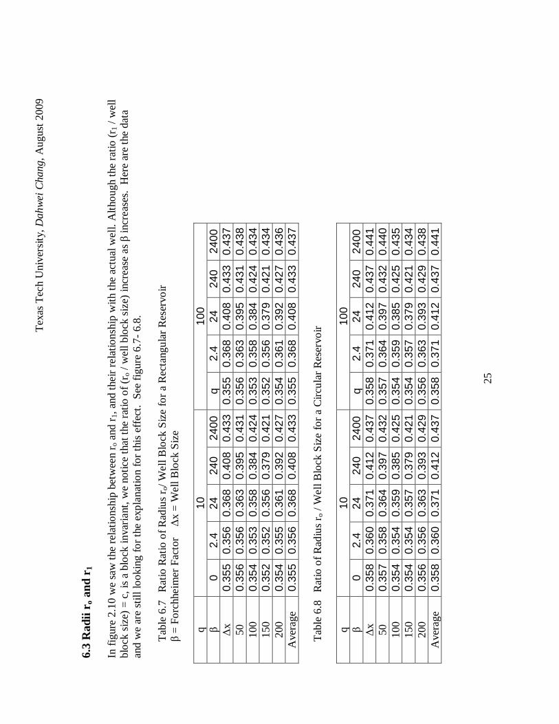
6.3

Rad

ii r o

and

r1

In f

igur

e 2.

10 w

e sa

w t

he r

elat

ions

hip

betw

een

ro

and

r 1, a

nd t

heir

rela

tions

hip

with

the

act

ual w

ell.

Alth

oug

h th

e ra

tio (

r 1 /

wel

l bl

ock

siz

e) =

c,

is a

blo

ck in

vari

ant

, w

e no

tice

that

the

rat

io o

f (r o

/ w

ell b

lock

siz

e) in

crea

se a

s β in

cre

ases

. H

ere

are

the

data

an

d w

e ar

e st

ill lo

oki

ng fo

r th

e ex

pla

natio

n fo

r th

is e

ffect

. S

ee fi

gure

6.7

- 6.

8.

T

able

6.7

R

atio

Rat

io o

f Rad

ius

ro/

We

ll B

lock

Siz

e fo

r a

Rec

tang

ula

r R

eser

voir

β =

Fo

rchh

eim

er F

acto

r ∆x

= W

ell

Blo

ck S

ize

q 10

10

0 β

0 2.

4 24

24

0 24

00

q 2.

4 24

24

0 24

00

∆x

0.35

5 0.

356

0.36

8 0.

408

0.43

3 0.

355

0.36

8 0.

408

0.43

3 0.

437

50

0.35

6 0.

356

0.36

3 0.

395

0.43

1 0.

356

0.36

3 0.

395

0.43

1 0.

438

100

0.35

4 0.

353

0.35

8 0.

384

0.42

4 0.

353

0.35

8 0.

384

0.42

4 0.

434

150

0.35

2 0.

352

0.35

6 0.

379

0.42

1 0.

352

0.35

6 0.

379

0.42

1 0.

434

200

0.35

4 0.

355

0.36

1 0.

392

0.42

7 0.

354

0.36

1 0.

392

0.42

7 0.

436

Ave

rage

0.

355

0.35

6 0.

368

0.40

8 0.

433

0.35

5 0.

368

0.40

8 0.

433

0.43

7

Tab

le 6

.8

Rat

io o

f Rad

ius

ro

/ W

ell

Blo

ck S

ize

for

a C

ircu

lar

Res

ervo

ir

q 10

10

0 β

0 2.

4 24

24

0 24

00

q 2.

4 24

24

0 24

00

∆x

0.35

8 0.

360

0.37

1 0.

412

0.43

7 0.

358

0.37

1 0.

412

0.43

7 0.

441

50

0.35

7 0.

358

0.36

4 0.

397

0.43

2 0.

357

0.36

4 0.

397

0.43

2 0.

440

100

0.35

4 0.

354

0.35

9 0.

385

0.42

5 0.

354

0.35

9 0.

385

0.42

5 0.

435

150

0.35

4 0.

354

0.35

7 0.

379

0.42

1 0.

354

0.35

7 0.

379

0.42

1 0.

434

200

0.35

6 0.

356

0.36

3 0.

393

0.42

9 0.

356

0.36

3 0.

393

0.42

9 0.

438

Ave

rage

0.

358

0.36

0 0.

371

0.41

2 0.

437

0.35

8 0.

371

0.41

2 0.

437

0.44

1

6.4 Degrees of Freedom Table 6.9 shows the degrees of freedom in our simulations. The circular reservoir has radius equal to 10000 which is larger than the rectangular reservoir of dimension 4000 x 8000. This is why our simulations for circular reservoir used more elements in the mesh, hence more degrees of freedom.

Degrees of Freedom Actual Well Simulation Rectangular Reservoir Circular Reservoir

3107 3412 Our Simulation Well Block Size

50 1699 2677 100 1346 2313 150 1219 2157 200 1176 2009


26

Texas Tech University, Dahwei Chang, August, 2009

27

CHAPTER VII

COMCLUSION

This work is for time independent. It may extend to time dependent initial

boundary value problems. The compressibility γ, usually the order of 10 -8, is ignored

in our calculation, this work may also be extended to include the compressibility in the

equation of state.

Another possibility for future work is to extend it to 3-D. The degrees of

freedom in our simulation are in the order 1000 – 2000. It only takes less than a

second to process on a modern computer. This may reduce the time when we extend it

to 3-D.

Texas Tech University, Dahwei Chang, August, 2009

28

BIBLIOGRAPY [1] Darcy, H. Les Fontaines Publiques de la Ville de Dijon, Dalmont, Paris, 1856. [2] Forchheimer, P. Wasserbewegung durch Boden Zeit, Ver. Deut. Ing. 45, 1901. [3] Peaceman, D. “Interpretation of Well-Block Pressures in Numerical Reservoir Simulation”, Society of Petroleum Engineers Journal of AIME, (Feb. 1978): 183 – 192. [4] Aulisa, E., Ibragimov, A., and Toda, M. “Geometric Framework for Modeling Nonlinear Flows in Porous Media, and Its Applications to Engineering, Nonlinear Analysis - Real World Applications”, Elsevier, Appear in 2009. [5] Aulisa, E. Ibragimov, A., Valko, P., and Walton, J. “Mathematical Framework of the Well Productivity Index for Fast Forchheimer (Non-Darcy) Flows in Porous Media”, COMSOL Users Conference 2006 Boston, Proceedings, http://www.comsol.com/academic/papers/1547.

PERMISSION TO COPY

In presenting this thesis in partial fulfillment of the requirements for a master’s

degree at Texas Tech University or Texas Tech University Health Sciences Center, I

agree that the Library and my major department shall make it freely available for

research purposes. Permission to copy this thesis for scholarly purposes may be

granted by the Director of the Library or my major professor. It is understood that any

copying or publication of this thesis for financial gain shall not be allowed without my

further written permission and that any user may be liable for copyright infringement.

Agree (Permission is granted.)

Dahwei Chang 7/02/2009 Student Signature Date Disagree (Permission is not granted.) ___________________________________ ____________ Student Signature Date

Peaceman’s Numerical Productivity Index for Non-Linear ...

Documents

Transcript of Peaceman’s Numerical Productivity Index for Non-Linear ...