pdf.usaid.govpdf.usaid.gov/pdf_docs/PNABI393.pdf · Transport . planning in developing countries....
249
Transport planning in developing countries. 380.5 ?-arral, Clell G. 42E ~a _ranst. D.anrdAg in developing countries '.. Iarra and rillo E. Kuhn. ijasrng¢, D.C., The Brookings Institution, transport Research Programn, 1965. 242 p. illus. Repas 5. l.Developing countries - Transportation. 2 .Transportation. I.Kuhn, Tillo E., joint author. II.Brookings Institution. II.Repas 5. IV.Title. TRANSPORT PLANNING IN DEVELOPING COUNTRIES by Clell G. Harral and Tillo E. Kuhn 1A.,r.. IST0,711TA, .AMT Transport Research Program The Brookings Institution Washington, D. C. June, 1965
Transcript of pdf.usaid.govpdf.usaid.gov/pdf_docs/PNABI393.pdf · Transport . planning in developing countries....
Transport planning in developing countries.
380.5 ?-arral, Clell G. 42E~a _ranst. D.anrdAg in developing countries
'.. Iarra and rillo E. Kuhn.ijasrng¢, D.C., The Brookings Institution, transport Research Programn, 1965.
242 p. illus. Repas 5.
l.Developing countries - Transportation.2 .Transportation. I.Kuhn, Tillo E., joint author. II.Brookings Institution. II.Repas 5. IV.Title.
TRANSPORT PLANNING IN DEVELOPING COUNTRIES
by
Clell G. Harral
and
Tillo E. Kuhn
1A.,r.. IST0,711TA, .AMT
Transport Research Program The Brookings Institution
Washington, D. C. June, 1965

Transport Planning in Developing Countries
CONTENTS
Part I. Techniques of Transport Planning
Page Chapter I. The Design of a Transport Study 1...................1
Chapter II. Problem Formulation ............ ....................... 8
A. Specifying the Transport Problem and Identifying Alternative Courses of Action ........................... 8
B. Economic Base Survey of the Area Affected ................ 11
Chapter III. Analysis of Present and Potential Traffic. ............. 17
A. Determination of Present Traffic Patterns ................. 17 Required Information ........................ 17 Sources of Information and Techniques of Analysis..... 26
(1) Compilation and Examination of Existing Data Sources 6..........................6
(2) Field Traffic Surveys: Vehicle Counts and Destination Surveys ....... .................... 28
(3) Sector Analysis ....... ....................... 31 Characteristics of Alternative Techniques and Suggested Usage ................................. 32
B. Methods of Traffic Projections ....... .................... 33
Chapter IV. Capacity of an Existing Transport System ................. 40
A. Required Information, Sources of Information, and Techniques of Analysis . ....................... 40
B. The Concept of Capacity and Its Role in Transport Planning.. ........................... 46
Chapter V. Estimating Benefits from Transport Investments ........... 50
A. Real National Income as a Measure of Benefits. .......... 50 1. The "National Income Benefits Criterion". ....... 50 2. Comparison of National Income Criterion With Costs
and Savings and Land Value Measures .............. 52 3. Advantages and Disadvantages of the National
Income Measure ........ ......................... 56

ii
Page B. Application of the National Income Measure of Benefits . . . . 58
1. Definition of the Economic Region Affected by the Proposed Investment .......................... 58
2. Projections of the Increase in National Income Which Would Result From Transport and Complementary Investments ........ ............................ 59
3. Determining Income: Netting out Purchases from Other Sectors and Regions. 2...................6
C. Examples of Actual Application of National Income Measures .......... .................................. 64
Example 1: Computing Increase in National Income by Deductible-Cost Method: El Salvador's Littoral Highway. ................................ 65
Example 2: Computing Increase in National Income by Percentage-Value-Added Method: The Cochabamba-Santa Cruz Highway ............................... 70
D. Summary .......... ................................... 80
Chapter VI. Appraisal of Costs and Determination of Alternative Technical Solutions ......... ............................... 83
A. Principles of Economic Costing .......................... 87 B. Transport Cost Components ....... ...................... 95
1. Capital Costs ........ ........................... 96 2. Maintenance Costs ............................... 98 3. Operating Costs. .......................... 98 4. Inventory and Other Costs. .................. 100
C. Estimation of Operating Costs: Sources of Information and Techniques of Analysis ............................. 102
D. Summary.......... . ................................. 106
Chapter VII. Decision Criteria for Choosing Among Alternative Investment Possibilities ........ ........................... 109 A. Financial Versus Economic Criteria. ................. 110 B. Formulating the Problem Correctly ................. 113 C. Uncertainties and Risks in Evaluating Costs and Benefits. . 118 D. The Investment Decision. ......................... 120
1. Computing present values of future benefit and cost streams ....... ......................... 120
2. Problems in the choice of a decision criterion ..... .. 122 3. Interdependencies, Alternatives, and the Formulation
of an Investment Program........................ 135 4. The Decision Rule ....... ........................ 137
E. Alternative Assumptions and Sensitivity Analysis .......... 148
Part II. Critique of Transport Planning Practices
Page Chapter VIII. Analysis of Pre-Investment Studies ............ 153
The Role of Pre-Investment Studies in Project Appraisal ... 156 Project Preparation and Evaluation in IBRD ........... 156 Project Preparation and Evaluation in AID ............ 158 Cost oi Pre-Investment Studies. ................. 160
Terms of Reference for Pre-Investment Studies ............. 162 The Project in Relation to the Economy ..................... 165 The Project in Relation to Other Transport Facilities ......... 167 Investment Analysis: Costs and Benefits .................... 169
Problems in Measuring Benefits ..................... 170 Problems of Cost Calculations ...................... 186 Other Problems of Benefit-Cost Analysis ............. 189
Conclusions .......... .................................. 190 1. Project Justification. ...................... 190 2. Failure to Relate Proposed Project to
the Economy ........................... 193 3. Underestimation of Project Costs ................. 193
Exhibit I: Survey Format ........ ......................... 194 Exhibit II: Terms of Reference for East African Road Project.. 200
Chapter IX. Time Lags in Transport Planning ................ 204 The Model ......... .............................. 204 Is the Investment Planning Process a Bottleneck? . .. .. . 209
Time Lags in the Investment Process: Empirical Evidence. . . 213 Duration of Investment Planning Studies .............. 214 Time Intervals in AID Investment Process ............ 219 Time Intervals Between First and Final
AID Disbursements ....... ....................... 225 Conclusions on AID's Investment Process Experience.. 233 Time Intervals: The Experience of the World Bank . . . 234
General Conclusions. 2.............................239

iv
LIST OF EXHIBITS
Exhibit Page
I. 1 Organization of the Transportation Study ............ 5
11.1(a) Area Economic Base Study - Natural Resources ....... 13
11.1(b) Population and Labor Force ..................... 15
11. 1(c) Industry Survey ......... ............................. 16
III. 1 Illustrative Time Profile of Annual Freight Traffic Through a Port by Commodity Classes ................ 20
111.2 Illustrative Origins and Destinations Matrix-Origins and Destinations of Salt Movements Originating in Madras State, March 1963 22...................2
111.3 Highway Freight Movements ........................... 24
111.4 Honduras Road Transport Origin and Destination Survey .......... .................................. 25
111.5 Sample Form for a Traffic Count ...................... 29
111.6 Highway Origin- Destination Survey Form ................ 30
111.7 Summary: Analysis of Present Traffic ............. 37
IV. 1 Highway Freight Movements 42....................4
IV.2 Capacity of Existing Highway System ............... 43
IV. 3 Summary: Appraisal of Present Transport Capacity ..... ... 49
V.1 Comparison of National Income Measure and Other Measures of Benefits ........ ........................ 54
V.2 El Salvador Cotton Production, Area, Quantity, and Price, 1953-54 to 1963-64 ....... ..................... 68
V.3 Production, Consumption and Import of Sugar, Bolivia, 1949-1962. 1..........................71
V
Exhibit Page
V.4 Estimated Rice Production in Bolivia, 1958-1963....... 72
V.5 Annual Gross Regional Product, and Portion Attributable to the Highway and Otner Investments, Santa Cruz Department, 1962 ......... ........................... 74
V.6 Capital Costs and Current Flow of Benefits, Cochabamba-Santa Cruz Highway and Associated Investments, Bolivia .......... .................................. 78
V.7 Summary .................................. 81
VI. 1 Illustrative Time Profiles of Costs for N-Year Planning Horizon .......... ................................. 97
VI.2 Summary: Determination of Alternative Technical Solutions and Appraisal of Costs ...................... 107
VII. 1 Net Present Value of Projects A 1 , A2 , A 3 , At Various Discount Rates ......... ............................ 133
VII.2 Analytical Weight of Future Benefits and Costs at Various Points of Time and Various Interest Rates ............. 144
VII. 3 Summary: Decision Criteria for Choosing Among Alternative Investment Possibilities .............. 151
IX. 1 The Development Project Planning and Action Process: A Generalized Presentation ........................ 205
IX.2 Duration of Investment Planning Studies ................. 215
IX. 3 Life Histories of Aid Projects ...... ................... 220
IX.4 Time Intervals in Aid Investment Process ............... 222
IX. 5 Random Sample of AID Loans Showing Time Span Between Loan Agreements and First and Final Disbursements... 227
IX.6 Suggested Shortened Project Planning and Action Process. 242
PART I
TECHNIQUES OF TRANSPORT PLANNING
by
Clell G. Harral

CHAPTER I
THE DESIGN OF A TRANSPORT STUDY
Transport seldom fulfills an independent function of its own; it serves
as a means to other ends. By moving people and objects for both economic
and noneconomic reasons, transport creates a link--political and social as
well as economic- -between people and objects separated in space. In so doing
it creates a value (or income), because the objects would not be transpor.ted
from one place to another unless their value after moving were at least as
high as before the movement took place plus the cost of transport. Similarly,
people would not move unless the worth to them of being in another place were
at least as great as the cost of the trip.
Improvements in transportation result in lowering real costs through
reductions in hauling costs, increased speed and dependability, decreased
losses and damages, or other means. Lowering real costs leads to savings
and increased production and consumption. The savings represented release
resources which may be applied to produce additional output elsewhere in
the economy. Or, they may be used in part to provide additional transport
services, since the reduction in transportation as a share in total costs tends
to result in the substitution of transport for other inputs. In this connection,
improved transport may bring about the employment of otherwise idle
resources; the classic example is the opening up of outlying lands.
Therefore, the benefits of prospective transport investment might be
measured by the extent to which they increase national income. Indeed, it
will be argued subsequently that a meaningful approach to the difficult
problem of measuring the benefits of alternative choices in transportation
lies in the income accounting concept of "value added." Certain imponder
ables will remain in evaluating social and political results, but itshould at
least be possible to assess the importance of noneconomic objectives in
relation to the cost of achieving them.
The demand for transportation usually arises because of spatial
relations involved in the production, distribution, and consumption of the
other goods and services. This forms the basic principle for all coordinated
transport planning at any level of analysis. In planning a national or regional
transport, system, or in appraising a single project, the underlying approach
and techniques of analysis will be the same.
The transport study must analyze the present and potential economy
of the area affected by the proposed development and the transportation
system which currently serves it. The existing geographic distribution of
economic activity is projected into the future, net supply and demand regions
for each major commodity are determined, and from these are inferred ex
pected future patterns of traffic flows. These projected transport demands
can then be compared with the existing transport system and the apparently
most important improvements identified.

3
In the second round of the analysis, the repercussions (or "feedback")
of the proposed transport improvements on the pattern of economic activity
must be estimated. Provision of a transport service is a complex matter
which requires many component parts, and changes in the system have wide
repercussions. For example, development of highway transport on any scale
requires feeder roads, vehicle fleets, and provision for maintenance. More
over, improvements in transport, whether in the form of reduced rates or
better service, may make new industries profitable and induce shifts in the
utilization of resources. These feedback effects are taken into consideration,
and then, once again, the most important transport improvements, given the
new pattern of economic activity, are identified. This analytical process is
repeated until the successive transport improvements lead to only minor
alterations in the economy and the most advantageous transport system is
determined.
This overall approach to transportation planning is discussed in detail
in subsequent chapters. The objective of the discussion is to: (1) determine
what information is required; (2) identify the likely sources of this informa
tion, and (3) develop the techniques of analysis to be applied.
It is inevitable that the scope of the studies and techniques suggested
here will not always be realized in practice. First, the list of important
factors, and therefore study requirements, will always differ from one case
to the next. Second, limitations on time, data, or the costs of the study will
4
often prevent accomplishing a wholly perfect realization of analytical goals.
However, the overall approach and many of the techniques of analysis proposed
here will still be applicable in any given case, although they may be used
less intensively.
Time, data, and cost constraints are often pressing, but restricting the
scope and depth of the analysis and thereby introducing increasingly broad
assumptions increases the likelihood of erroneous conclusions. This dilemma
may be solved, in part, by selective emphasis. Clearly it is important that
those assumptions and estimates which affect the outcome of the investment
decision should be more carefully considered than those which do not have
much effect on the outcome. Fortunately, there are simple and effective tech
niques of "sensitivity analysis" for determining the importance of various
components of the investment analysis. A later section of this manual discusses
these techniques.
Moreover, while the costs of competent pre-investment studies may be
quite substantial, there are indications that the costs of good studies are no
higher than those of poor studies. In any event, the costs of pre-investment
studies compared to the physical investments proposed are quite modest.
The basic steps of a transport planning study are outlined schematically
in Exhibit 1.1. of any transport planning study isThe first stage to define the
main sources of traffic or demand for transport services. This is done by
attempting to estimate present and potential future demand as derived from
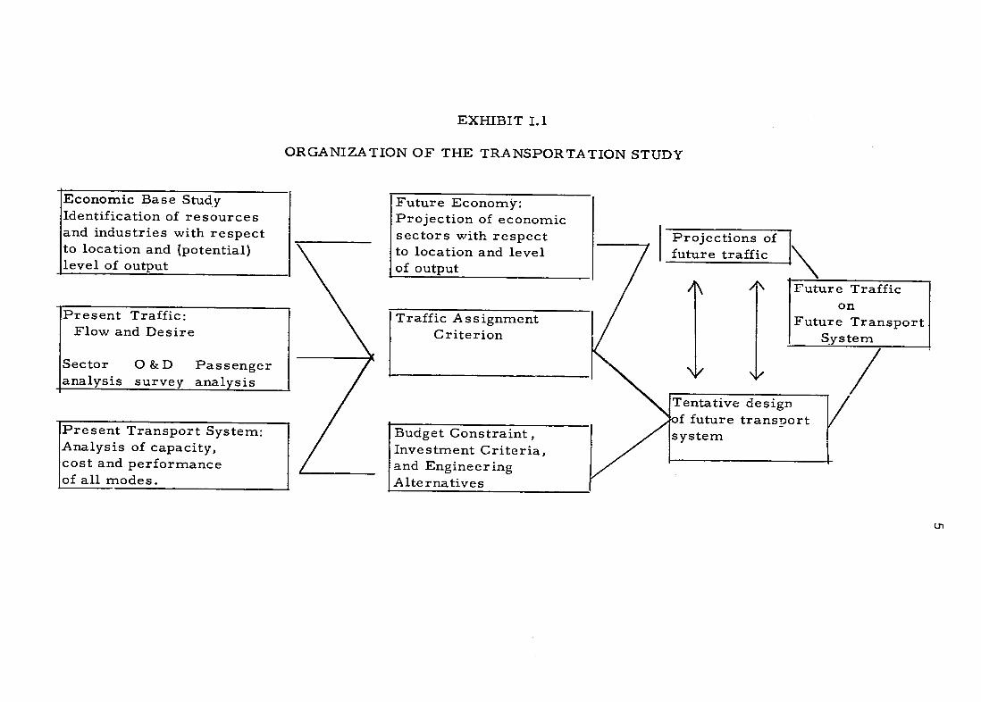
EXHIBIT 1. 1
ORGANIZATION OF THE TRANSPORTATION STUDY
Economic Base Study Future Economy: Identification of resources Projection of economic and industries with respect sectors with respect Projections of L to location and (potential) to location and level future traffic N level of output of output
2 I\ Future Traffic on
Present Traffic: Traffic Assignment Future TransportFlow and Desire Criterion System
Sector O&D Passenger N/ analysis survey analysis
Tentative designof future transport Present Transport System: Budget Constraint, system Analysis of capacity, Investment Criteria, cost and performance and Engineering
,of all modes. Alternatives
U.n

6
the economic activities which use transport services. Ordinarily, an economic
base survey is required which includes an appraisal of the natural resource
base, the population and labor force and the existing industries of the area
under consideration including the social structure, attitudes and incentives of
the people. The purpose of the base survey is to identify those industries
which will be the main users of the transport facilities, such as agriculture,
forestry, mining, manufacturing, and foreign trade, and to specify their present
and potential future location and level of output.
This base study should be complemented by a detailed analysis of
present traffic which will result in a map of both the actual flows over the
existing transport network and the desired flow routing based on origins and
destinations. This requires a two-part study: (1) direct traffic survey--traffic
counts, 0 & D surveys, and bill-of-lading studies; and (2) an extension of the
sector survey techniques to infer transport flow platterns from the geogra
phical distribution of production and consumption points, and the technical inter
industry relationships.
The third major part of the analysis centers on the supply side, on the
assessment of the capacity, cost and performance of the existing transport
system. This three-pronged attack provides the thorough understanding of
the existing situation necessary for a meaningful projection of the future
economy and its transport requirements. It is only when this projection has
been accomplished that the combined economic and engineering analysis
described earlier can be undertaken. Repeated "loops" or rounds of analysis

7
can be used to simulate the reaction of the future economy to possible (hypo
thetical) changes in the transport system and their repercussions back again
on the transport system. Usually only a limited manageable number of such
analytical rounds are required to arrive at a preferred design for the future
transport system.

8
CHAPTER II
PROBLEM FORMULA TION
A. Specifying the Transport Problem and Identifying Alternative Courses of Action
Transport investment proposals may originate at the official request
of the government of the host country, an unofficial request of a member of
that government, or through individuals or groups of citizens of that country.
They may also be directly initiated by personnel of United States and inter
national agencies within the country concerned. These requests may be results
of the well-reasoned recommendations of countrywide transport planning
surveys, or other smaller scale transport studies; or they may represent the
implementation of economic plans at the national, regional, or local level.
However, they may simply reflect an immediate reaction to obvious transport
problems and a decision to act upon them quickly in one way or another.
Because the engineering and economic issues are so complex, even an
intelligent, informed, and personally disinterested observer is seldom able to
suggest the most desirable solution to a given transport problem without
expert and detailed study. -The sponsor of a particular solution may be unable
to foresee consequences which would occur elsewhere in the economy. A
sponsor may not know the alternative uses to which the public investment
funds could be put, and therefore he will not be in a position to assess the
9
given proposal in terms of the overall priorities of the country's develop
ment program. And, of course, it may be that the party favoring a particular
proposal is not disinterested and has objectives which neither a lending
agency nor the best interests of the investing country would recommend.
In this situation it is the duty of the analyst to review the transporta
tion proposal within the framework of the objectives of the lending agency and
the host country. He should take account of the overall schedule of priorities
in the country's development program, and the specific transport problem
which gives rise to the proposal. It is essential that the real transport
problem be specified and the effective alternatives identified. The problem
may be one of the following: penetrating and opening up an area which is
inaccessible during part or all of the year; increasing seasonal capacity
which is saturated during peak periods of the agricultural season; reducing
the distance between two urban centers; improving the quality of passenger
services, or reducing port handling costs. In any case, specifying the purpose
of the proposed project will help the analyst to identify alternative solutions
and to weigh their costs and benefits. This may be a simple task, with a few
effective alternatives which are easily identified by an economist upon pre
liminary examination. In other cases it may be very difficult, and ultimate
specification of the engineering and economic alternatives will constitute a
large part of the expert's task. However facile or difficult, it is only when
the costs and benefits of alternative courses of action are made explicit
10
that it is possible to judge the merits of any proposed project. If there are
no alternatives, there appears to be no problem, and no need for analysis.
But, in fact, there will always be the alternative of doing nothing- -often a
realistic alternative which must be examined.
Alternative solutions to transport problems should not be confined
to physical investments. They should ordinarily include at least five broad
groups of possible changes:
(1) Changes in present administration and regulations
which would increase the effective capacity of the
existing system;
(2) Rationalization of present rate and tariff structures
toward more efficient utilization of transport
services;
(3) Improvements in operational efficiency and coordin
ation of existing facilities;
(4) Alterations in plans for the location of industry,
the concentration of electric power production, and
transmission by high voltage lines, development of
processing and containerization practices, storage
facilities, and telecommunications networks;
(5) Capital investments to increase the physical capacity
of the transport network, including entirely separate
and perhaps radically different solutions from the
original proposal as may be evidenced in cases
involving a choice of mode among road, rail, air
and river or coordinate development of two or
more of these modes.
B. Economic Base Survey of the Area Affected
The appropriateness of a transport investment will be determined
by the volumes and characteristics of the traffic which ultimately uses
the facility. Therefore, an economic resource survey of the area where
transport improvements are contemplated must be made. Such a survey
will encompass three broad elements:
(1) Survey of productive potential, including both
physical and human resources.
The objective of the productive potential resource survey is to
obtain a general land potentialities or capabilities mapping. Land capabi
lities is a composite function of many separate variables. The major
physical factors are outlined in part (a), the human factors in part (b), and
the industrial infrastructure factor in part (c) of Exhibit II.l. Any one of these
factors by itself will have little meaning for economic planning. Only when
they are all integrated by an expert economic geographer into a land
capabilities mapping do they become a usable tool of economic analysis.
An important example of land capabilities analysis used for economic
development planning is cited in the notes to Exhibit I.(a).
(2) Survey of market potential.
(3) Survey of "entrepreneurial potential," or the response
of the economy to profit-making opportunities, including
government and private investment plans.
If the physical potential, the natural resources, and the labor does
not exist, certainly no goods can be produced, and no traffic can develop.
If the market does exist, or no investment is forthcoming, no production
and traffic will result.
This type of survey will ordinarily require employing an expert
economic geographer or team of experts with a background in demography,
natural resources, agriculture, forestry, and manufacturing industries who
can analyze both productive potential and market potential.
The accompanying Exhibits II. 1(a), (b) and (c) depict the important information
required and the likely sources of this information under three general
classifications: (a) natural resources, (b) population and labor force, and
(c) industries.

EXHIBIT 11.1(a)
AREA ECONOMIC BASE STUDY
Natural Resources*
Subject Informati-)n Required Source of Information Purpose of Information
Ecological Contour mapping of land surface; hydroelectric mapping of water and drainage system.
Basic information often available in published maps. Detailed information for advanced planning stages,
A major determinant of the level of cost (capital, maintenance, and operating) and the choice of mode.
such as highway location, to be derived from engineering, aerial, and land survey.
Mapping of rainfall zones according to annual totals and description of monthly pattern; profile of tempera-ture ranges by zones. Inte-gration into composite
picture of climate and effect on economic activity.
Published sources, records of meteorological depart-ments of governments and universities,
Determinants of levels and patterns of agricultural production; and the capital, maintenance and operating costs of transportation and quality of service.
Geology (Building Materials)
MVapping of rock formations: locations and quantifications of stone and sand aggregates. Determination of geologic structure for construction of right-of-ways,
General information avail-able in published sources, government and private surveys, or direct interview of engineers and local sources. Detailed informa-tion requires expert survey and analysis techniques.
Location in appropriate quantities of building materials, a major determinant of construction costs. Geologic structure of right-of-way a fundamental determinant of costs of excavation.

EXHIBIT II.l(a)
Subject
Minerals
Soils
Vegetation
Energy Sources
- continued
Information Required
Mapping depicting locations and quantifications of mineral deposits. Appraisal of economic potential, in-cluding known outputs and plans for future exploitation,
Mapping depicting soil zones for both agricultural and engineering classifications,
Mapping of major vegetation zones, particularly forests and grasslands. Survey of forest reserves and assess-ment of economic potential, including plans for development.
Location and economic evalua-tion of actual and potential
sources of energy: hydro-electricity, thermal electricity, coal, petroleum, and natural gases.
Source of Information
Expert appraisal, involving both qualitative analytic and field survey techniques essential. This will already be available, or will be undertaken directly, or qualitative impressions must form the basis for appropriate assumptions.
General information available in published and government sources. Otherwise requires expert analysis and survey techniques.
Published sources, govern-ment and university agricul-tural and forestry depart-ments, and private lumber companies.
Published surveys; govern-ment authorities; private and public power, coal mining, and petroleum companies.
Purpose of Information
A major determinant of potential traffic.
Determinant of agricultural demand for and construction costs of transportation investments.
Timber potentials often a major determinant of traffic. Grasslands important to determination of levels and patterns of farming and animal husbandry.
Major determinant of level and pattern of potential economic development.
*-Anoutstanding example of resource inventory analysis for development planning is given by the Department of Economic Affairs of the Pan American Union, Survey for the Development of the Guyas River Basin of Ecuador: An Integrated Natural Resource Evaluation (Washington: Organization of American States, 1964).
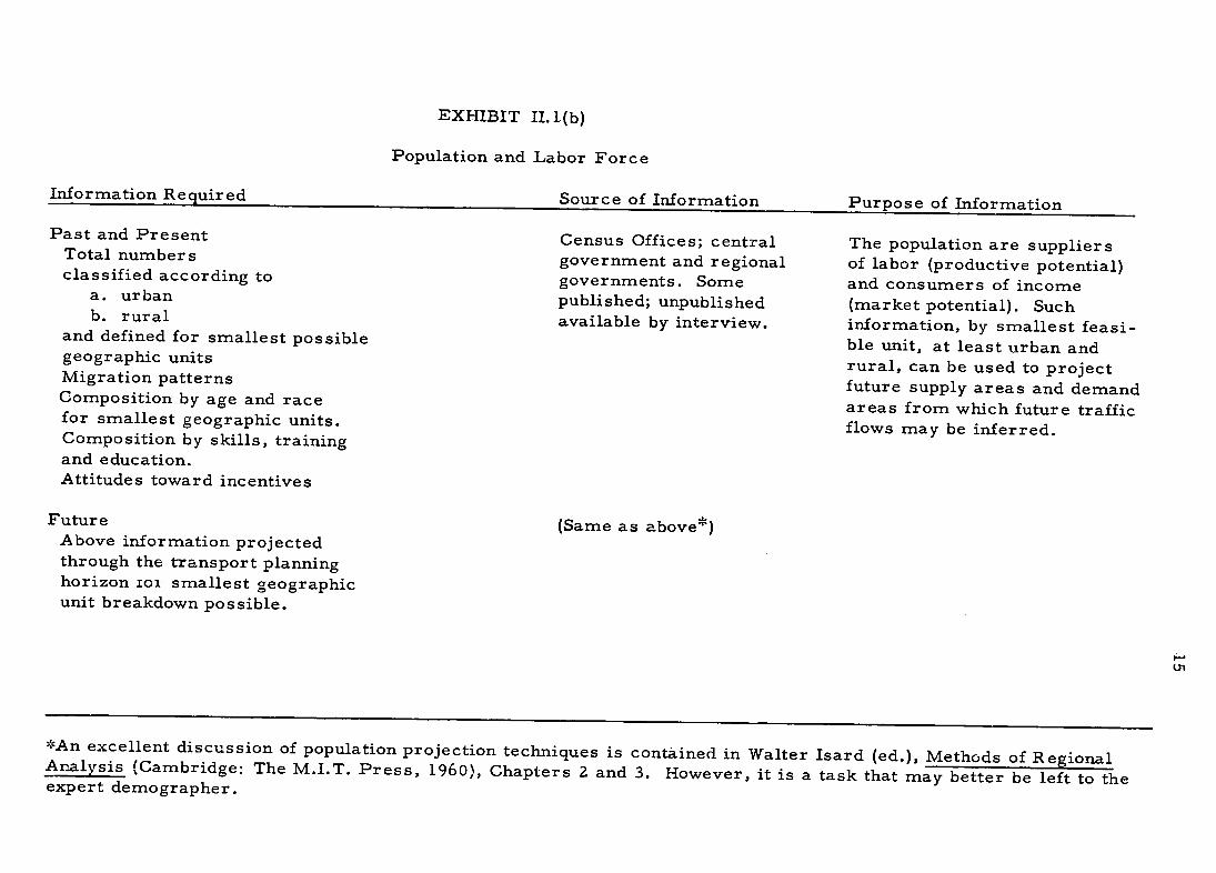
EXHIBIT II.I(b)
Population and Labor Force
Information Required Source of Information Purpose of Information
Past and Present Census Offices; central The population are suppliersTotal numbers government and regional of labor (productive potential)classified according to governments. Some and consumers of income
a. urban published; unpublished (market potential). Suchb. rural available by interview. information, by smallest feasiand defined for smallest possible ble unit, at least urban andgeographic units rural, can be used to projectMigration patterns future supply areas and demandComposition by age and race areas from which future trafficfor smallest geographic units. flows may be inferred. Composition by skills, training and education. Attitudes toward incentives
Future (Same as above*) Above information projected through the transport planning horizon ioi smallest geographic unit breakdown possible.
u1
*An excellent discussion of population projection techniques is contained in Walter Isard (ed.), Methods of RegionalAnalysis (Cambridge: The M.I.T. Press, 1960), Chapters 2 and 3. However, it is a task that may better be left to the expert demographer.

EXHIBIT 11. 1(c)
Industry Survey
Information Required Sources of Information Purpose of Information
Identification and mapping of important traffic generating industries, including agriculture. Determination of total inputs and outputs classified by commodity in physical terms with location of markets and suppliers specified in greatest possible
Previous surveys, published and unpublished. Census of manufac-tures, industrial directories, even telephone books,
Agricultural ministries, missions,
Determination of the geographic distribution of supply points on the one hand and markets on the other, can be used to infer traffic flow patterns.
detail. extension agents, etc.
Commodity flow studies: -ailroad; trucking, port statistics.
Field surveys: questionnaires and direct interviews with government, planning, and industry officials.
Appraisal of governmental and private plans for development.
a,

17
CHAPTER III
ANALYSIS OF PRESENT AND POTENTIAL TRAFFIC
A. Determination of Present Traffic Patterns
Describing and analyzing traffic patterns on an existing transport
system in one of the most direct and effective tools of transportation planning.
It serves two functions: (1) It forces identification of the major determinants
of existing traffic, which not only contribute substantially to an understanding
of the functioning of the present economy, but also provides an essential base
for sound projections of the future level and geographic distribution of eco
nomic activities, as well as the allocation of future traffic between alternative
modes of transportation. (2) It permits comparison of present transport
demand with the existing transportation system and assessment of present
and potential problems of capacity.
Required Information
Transport planning requires information on present level, seasonal
pattern, and trend over time of transport demand for both freight and passen
ger services in the area concerned. Demand should be stated in terms of
desired orgins and destinations as well as actual movements. Desires for
traffic flow are the correct measure of transport demand for planning pur
poses. Actual movements reflect how these demands are worked out on the

18
existing network of highways, railroads, airways, and waterways. When
information on desire flows is integrated with actual traffic movements in
a composite analysis, essential information about the functioning of the
present economy and its transport network can be inferred.
Traffic information must depict actual and desired movements in
terms of physical quantities (freight tonnages and numbers of passengers)
specgfied with respect to the location, commodity classification, and timing
of the movement.
I.. Physical quantities. Transport demand analysis must describe
the physical flows to be accommodated in terms of tonnages of goods and
numbers of people. It must be more than a mere count of the number of high
way vehicles, aircraft, railway cars, and similar "containers" used for
movement. The fact that capacities and load factors of vehicles or containers
vary widely limites the utility of this kind of statistic: a simple traffic count
without reference to the structural composition of the vehicle fleet is only one
step removed from no information..
2. Location of the movement. The spatial element is one of the dis
tinguishing characteristics of transportation: movement of a ton-
of a particular good from one point A to another point B is a very different
service from movement of that same ton. from point C to point D-
indeed, it is even quite different from the reverse movement of that
same ton from point B to point A. A similar statement applies to location
of the transport facilities which provide these services.

19
Statements of aggregate tonnages, ton-kilometers, or tonnage originat
ing without reference to the specific routing of these movements are without
utility for all but the most limited transport planning purposes. Only when it
can be specified that a certain amount of traffic was carried over a particular
segment (or segments) of the system, which had a certain capacity, is it
possible to infer that measures to expand capacity are or are not desirable.
3. Commodity composition. It is ordinarily desirable to distinguish
the commodity composition of traffic for two kinds of reasons cited in the
opening paragraph to this section: to identify the individual components of
present traffic in order to facilitate projection of future traffic and in order
to allocate that traffic between alternative modes of transportation. Usually
a limited number of commodities will constitute the great bulk of the traffic.
4. Time profile. Demand for transportation will fluctuate widely
over the seasons:of the year, and it is necessary to identify this time profile
in order to determine the exact nature of transportation requirements. Weekly
and even daily variations can be important in certain cases. The appropriate
response to a given level of transport demand will vary widely for different
time patterns of the demand. For example, the movement of agricultural
commodities which is particularly subject to seasonal peaking, may be most
efficiently accommodated in part by nontransport measures, such as storage,
processing, and containerization. Where possible, it is most desirable to
determine a monthly profile of t1he traffic movements, such as is given in
Exhibit 111. 1.

EXHIBIT 111.1
ILLUSTRATIVE TIME PROFILE OF ANNUAL FREIGHT TRAFFIC, THROUGH A PORT BY COMMODITY CLASSES
Commodity Dec. 1962
Jan. 1963
Feb. 1963
Mar. 1963
Apr. 1963
May 1963
June 1963
July 1963
.Aug. 1963
Sept. 1963
Oct. 1963
Nov. 1963
Agricultural and Food Products
Household Goods, Personal Effects
Fuel, Oil
Industrial Products
Miscellaneous
1320.4
142.3
148.9
72.4
13.5
1026.2
65.8
52.4
115.9
31.2
974.4
53.3
10.0
79.3
6.4
1104.4
25..4
100.6
98.0
36.6
585.2
41.2
127.5
46.8
31.1
298.6
33.7
141.0
55.8
0.0
476.3
56.8
32.5
32.8
29.6
497.8
52.5
206.7
130.1
9.2
696.8
21.2
38.4
161.2
109.0
545.9
8.4
327.3
83.4
0.0
809.8
6.2
88.9
68.6
10.9
881.4
113.0
79.2
149.2
0.0
Totals 1697.5 1291.5 1123.4 1365.0 831.8 529.1 628.0 896.3 1026.6 965.0 984.4 1222.8
GRAPH OF TIME PROFILE (Figures correspond to aggregate monthly totals above)
1850-1700-1550-1400-1250-1100-
950-800-650-500-
May June July Aug. Sept. Oct. Nov. Dec. Jan. Feb.
-1850 -1700 -1550
- z1400 1250 -1100
-950 800 650 500
Mar.
21
The objective of traffic analysis is to obtain as complete a statistical
description as possible for both the present and previous patterns of traffic
movements in terms of the four characteristics just discussed. Assuming,
at this point, that the data are available this will result in two collections of
data:
(1) For each segment of the transport system in the area
concerned, the amount of freight tonnage classified by
commodity type, and the number of passengers for each
month of the year.
(2) A matrix depicting desired orgins and destinations for
physical flows of freight and passengers, for each (major)
origin and destination in the region, including import
and export points for extra-regional movements.
Two illustrations of such collections of data are presented in Exhibits
11.l and 111.2. Exhibit III.1 depicts a time profile of physical movements by
commodity classes for an East African port during year, 1963.one This is
a useful piece of information in itself, but ideally it would be only one of a
very large group of such statistics depicting the same information for every
segment of the transportation system concerned. Exhibit 111.2 illustrates a
matrix of desired origins and destinations for the movement over all modes
of transport of a particular commodity during some one-month period. The
figures in this case are strictly fictional, but the names of places are drawn

EXHIBIT 111.2
ILLUSTRATIVE ORIGINS AND DESTINATIONS MATRIX-ORIGINS AND DESTINATIONS OF SALT MOVEMENTS ORIGINATING IN MADRAS STATE, MARCH 1963
(In thousands of tons)
Destinations
MadhyaOrigin Andhra Assam Bihar Bengal Kerala Maharashtra Pradesh Mysore Orissa Total
Tanjore and S. Arcot 1481.8 -- 119.0 .... 1764.8 24.3 3389.9
Tirunelveli and Ramnathpuram 604.0 140.6 6958.0 15121.0 3077.0 18.0 264.0 2334.0 2324.0 17240.6
Kanya Kumari .. .... .. 1065.2 .... 1065.2
Total: 21695.7
*Data are illustrative only.
EV
23
from an actual study, which encompassed 483 possible origins and destinations
for 32 commodity classifications- -and resulted in an enormous mass of
valuable information.
The interpretation of data in this quantity and with these characteristics
is greatly facilitated by presentation in a mapping format. Mapping techniques
as a method of economic and geographic analysis are well established and
particularly suited for the problems of transport analysis.
The various characteristics of traffic statistics can be combined and
reduced to a visual representation which combines vast quantities of informa
tion in a concentrated, easy-to-use form. It presents the data in an effective
and readily understood form to those officials and others who must use the
report but who are not directly concerned with the analysis, and it can also
constitute a technique of analysis, especially for wide-scale transport surveys.
Parallel mapping of the capacities of the present or anticipated transport
system can be constructed, the traffic and capacity maps overlaid, and actual
or potential bottlenecks determined (see Chapter IV).
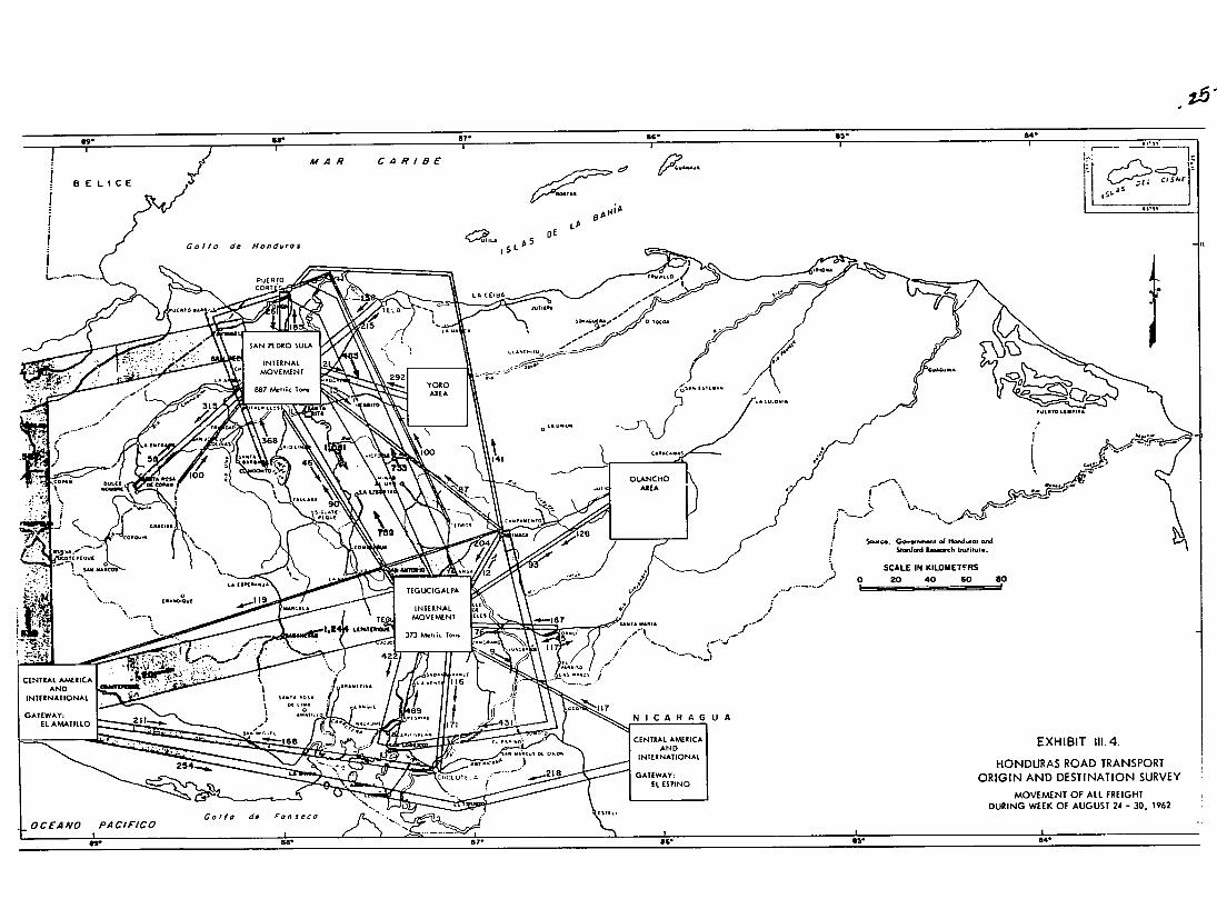
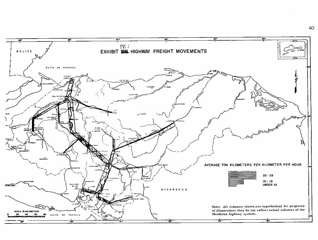
Exhibits 111.3 and 111.4 present examples of useful traffic mapping
taken for purposes of illustration from a recent highway transport survey of
Honduras. The information in Exhibit 111.3 depicts estimated annual freight
flows as derived from detailed traffic surveys. The width of the ribbons indi
cates the level of the traffic flow, in metric tons, over the existing highway
net-work. Exhibit 111.4, on the other hand, shows the result of a detailed highway

LL
4 *-B5*66.1511 Or-
CISNFREIGHT MOVEMENTSBEL I CE EXHIBIT 111.3. HIGHWAY
Golfo de HOndurOS
L... -.... PUERT0 CORTE L
!C I 01011,
Outti otC flo
•op. .,.I
~~ ~~.,, ..
E , .............. .
AVERAGE TON KILOMETERS PER KILOMETER PER HOUR
20- 39
..... : U1,NDER 0 I ,.O ,L , IN I C A R A G U A
Note: All volumes shown are hypothetical for purposes
of illustration; they do not reflect actual volumes of the"ILOMETERSSCALE IN ,,.. Honduras highway system.0 20 40 -60 0 Go/to de
II B-
I L
"88*
MAR c AR o -e ? 86 5* 64* i:
IdAACA RIB R
Go~~~~~ 11EeHn~,SL
SA 5
PUERTO CORT -
LA CEIBA-
SAN PEDRO SULA A'NIRAL .. daa,
MCI.
.......... ... !7 S
INT1 ENAL o
'' .s = . .o ' " -. )3 :t.SCALE IN KILOUETFRS
T MOVEMENT - ~ -.e---167 AA°
CLAN -t
CENATA L A. 88ra 87" 14.1.. 8G*213 o
84
GATEWAY: ELAMATIL.O 22..,
I 1- L*
N0I89
I A
A R A.G U7
A U
c,,m"wt'j j,.,cA"
.... " '*INTERNATIONAL
GAT[WAY:
HONDURAS ROAD TRANSPORT ORIGIN AND DESTINATION SURVEY
:' i'"L E.PINO
" " MOVEMENT OF ALL FREIGHT
OCEANO PACIFICO W
Go-.d ans
S
oIDURING B"...
I
WEEK OF AUGUST 24 - 30, 1962 ,

26
origin and destination interview survey, the ribbons indicating the desire
flows from origin to destination. Here the information is not how freight
actually does flow, but how it would like to flow. This represents genuine
point..to-point highway freight transport demand in Honduras, given the
existing transport system and the resulting distribution of economic activity.
(Of course, future demands, or "flow desires," will be affected by any sub
stantial alternations in the existing network. See Chapter III.B.) It is
ordinarily desirable to summarize present traffic information in this ofk a
similar mapping format, whether for the study of an entire transport system or
only a short . section of highway, railway, or other mode.
Sources of Information and Techniques of Analysis
Development of required traffic statistics will usually require a com
bination of three broad techniques: (1) compilation and examination of all
existing data sources; (2) direct generation through field traffic surveys; and
(3) inference from sector or industry studies involving both interview and
questionnaire surveys and technical "industrial complex" analyses. The
method of analysis to be used in any given case will depend on the nature of
the problem, the availability of data, the scope of the study, and time and cost
constraints.
(1) Compilation and Examination of Existing Data Sources
Necessary information will ordinarily be available in some form for both
actual movements and desired origins and destinations,, rail., air, and ocean bound
27
traffic (both freight and passengers), from bills of lading and ticket records
in railway, airline, and shipping companies and from port authority files. In
some countries this information will be almost nonexistent while in others
it may be complete and detailed and extend back over several years. It may
already be available from the railroad and airline companies in an immediately
usable form suitable for mapping; but in most cases laborious tabulation
directly from the original forms will be required.
Determining highway traffic, often a major component of the analysis,
may involve examination of available data sources but chief reliance must
commonly be placed on direct field surveys (including aerial photography).
Some data may be available from permanent local octrois, weighing stations,
border crossings or police checkpoints. If (and only if) the reliability of
these data can be verified from independent sources and estimates, they are
useful for determining patterns of seasonal fluctuations in traffic, and even
long-term trends. Rarely, however, will they provide an adequate description
of total traffic flows by themselves; since the stations were conceived and
established for a function distinct from traffic analysis, their records ma,
at best record simple counts of all traffic. Sometimes they will refer only
to certain categories of traffic (such as trucks, or heavy trucks, but not
passenger cars, buses, or animal-drawn vehicles), and, moreover, the check
posts may be too far apart to obtain a complete picture of traffic. Finally,
records of local checkposts rarely yield information on desired origins and
destinations, as opposed to actual flow patterns.

28
(2) Field Traffic Surveys: Vehicle Counts and Origin and Destination Surveys
a. Traffic Counts. Traffic counts involve a simple enumeration of
vehicles for each hour of the day, preferably distinguishing among passenger
cars, buses, trucks of each capacity, animal-drawn vehicles, etc. In each
direction of movement, they should distinguish among types of commodities
carried among empty, loaded, or partly loaded trucks. They can be conducted
by aerial photography, or by stationing human observers or mechanical
counters at as many strategic points as necessary to determine traffic
patterns in the desired detail. Traffic counts offer the important advantages
of simplicity-and low cost, but they are subject to the severe limitations
discussed earlier on page .18. Exhibit 111.5 shows a sample form for recording
vehicle count which was designed for use in an actual traffic count. Local
police were employed as counters. Because some of them were illiterate, it
was necessary to include pictures of the various vehicle classifications.
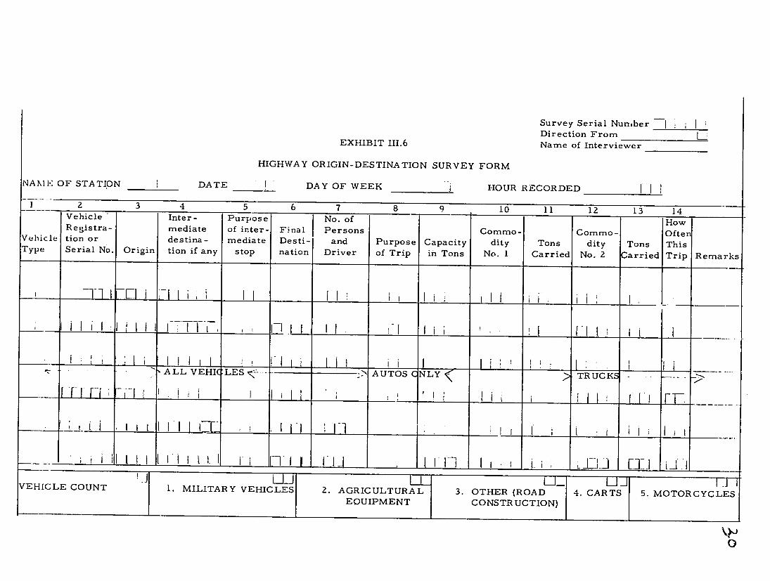
b. Origin and Destination Surveys. For origin and destination
surveys (0 & D), traffic interviewers, who have had at least some briefing on
their tasks, are placed at strategic checkpoints on the transport network
with facilities (and authority) to stop each vehicle, or some percentage sample
of vehicles. The interviewer ordinarily will be instructed to obtain informa
tion on origins and destinations for each commodity hauled, tonnages of each
commodity, type of vehicles, number of passengers, and other information.
Exhibit 111.6 gives a sample format for an origin and destination interview

EXHIBIT 111.5
SAMPLE FORM FOR A TRAFFIC COUNT
SERIAL NO ............. TRAFFIC COUNT ROUTE ...................
TYPE OF VEHICLE
LOCATION ..............
SI I
Heavy Truck & Trailer
i0
Trucks & Buses
I Light Trucks
Landrovers & Cars
ATE
DAY 0600-1800 Hours
Direc-tion From: To:
NIGHT 1800-0600 Hours
DAY 0600-1800 Hours
Direc-tion From:
To:
NIGHT 1800-0600 Hours
DAY 0600-1800 Hours
Direc-tion From:
To:
NIGHT 1800-0600 Hours
Type of Cargo Number of Passengers [ REMARKS
TOTALS_
_______
Survey Serial Number Direction From Li
EXHIBIT 111.6 Name of Interviewer
HIGHWAY ORIGIN-DESTINA TION SURVEY FORM
NANII, OF STATION DATE [ DAY OF WEEK j HOUR RECORDED I ]
1 2 3 4 5 6 7 8 9 10 11 12 13 14Vehicle - Inter- Purpose No. of HowRegistra- mediate of inter- Final Persons Commo- Commo- OftenVehicle tion or destina- mediate Desti- and Purpose Capacity dity Tons dity Tons ThisType Serial No. Origin tion if any stop nation Driver of Trip in Tons No. 1 Carried No. 2 Carried Trip Remarks
__I~-!_ Il , I I I1 I I i i l l , lI, I
____________________________,,_,__ -7**Ii I I I I I i i, 1 I
,i_ il K 1K ii_~~l _ _ALL VEHI LES - AUTOS NLY,-
, TRUCKS
_______--i ai.... Z LJ i F TRil . [I]K . .... ____- _
-IU LVEHICLE COUNT LiI j -.1. MILITARY VEHICLES Z. AGRICULTURAL 3. OTHER (ROAD 4. CARTS 5. MOTORCYCLES EOUIPMENT CONSTRUCTION)
0

31
requiring certain information, all of which can be contained, in coded form,
on a computer card.
(3) Sector Analysis
Analyzing individual industries, major plants, and activities offers an
indirect approach to determining traffic flows which may serve as a supple
ment (or, rarely, an alternative) to direct traffic surveys. There are two
major components of the sectoral approach: interview and questionnaire
surveys, and technical complex analysis.
Well-conceived and properly executed interviews and questionnaires
from major transport users and public carriers can be made to yield reliable
information on transport patterns, sometimes for a large majority of tr ,fic.
They should be so designed as to include internal consistency checks and
permit cross-checking between different sources. Coverage should be as
complete as possible, and where sampling is required, sound statistical tech
niques should be applied.
Industrial complex analysis for traffic studies requires first the deter
mination of levels of industry or plant outputs with location specified. Techni
cal input coefficients, known from engineering technologies or determined
from a census of manufacturing or other industry studies, are then applied
to determine the (physical) amounts of the various inputs required for the
specified levels of output. Knowledge of potential input suppliers and market
outlets are then analyzed using comparative cost and location techniques to

32
determine likely traffic flows. These estimates can then be cross-checked
and reconciled with the results of questionnaires and direct traffic surveys.
Valuable information on the preference of various industries for alternative
sources of supply and modes of transport may be inferred.
Characteristics of Alternative Techniques and Suggested Usage
Traffic information required for transport planning was described in
the opening paragraph of this section; various approaches to the determination
of this information have been outlined above. Each approach is appropriate
for specific purposes, and each has its advantages and disadvantages.
Ideally, the various techniques will be integrated and employed in a
systematic manner to develop a coherent and balanced picture of transport
demands in the area concerned. Present levels of actual flows are most
easily determined using a combination of currently published carriers'
statistics and traffic surveys. Desired commodity flows by origins and
destinations will be determined from examination of carriers' bills of lading
and tickets, and the direct undertaking of origin and destination surveys.
Secular trends will be available from the published carriers' statistics or
can be established from questionnaires (including interviews) to the major
transport shippers and carriers; and, similarly, the patterns of seasonal
fluctuations will be determined frorr the published statistics of the carriers,
highway checkpost records, and industry questionnaires, supplemented on

33
occasion by correlation with statistical series for petrol consumption. Thus
for any one transport study it may prove necessary to use all of these tech
niques, and still others improvised by the analyst to fit the situation, to
provide cross-checks on the various sources of data, and thus obtain a meaning
ful description of traffic.
In some situations this will be a costly and time-consuming task, and
the transport analyst will undoubtedly have to use his judgment to obtain a
rational balance between data requirements on. the one hand and the time and
money costs of compilation on the other.
A summary description of the required information and some of the
methods discussed above is presented in 'Exhibit 111.7.
B. Methods of Traffic Projections
Extrapolation of past traffic growth rates, or equations of the
growth of traffic in small regions with the overall rate of growth of traffic for
the whole nation, are grossly oversimplified techniques which can easily lead
to wholly fallacious traffic projections. Traffic can develop only where the
resources and market potential exists and the necessary investment of capital
and amangerial talent is forthcoming to convert the potential into actual in
creases in agricultural, forestry, mining, and industrial output.
The detailed description of the present economy--the natural resources,
the spatial distribution of industry and population--and the resulting traffic
desires and actual flows over the existing network / combined with a careful
_/ Discussed in Chapters II.B and III.A above.
34
evaluation of governmental and private investment plans, provide the essen
tial basis for sound traffic projections. Indeed the information required
about future traffic is the same as that required for present traffic: mapping
of the level and seasonal pattern for both desired origins and destinations
and actual routings by commodity classifications. J
_ See Chapter III.A above, pp. 17-26.
Moreover, the basic techniques of projecting future traffic is an
extension of the techniques of "sectoral analysis" used in determination of
present traffic patterns. The economic analyst in close cooperation with the
engineer must determine two important pieces of information;
i. The location of each proposed transport facility;
ii. The likely unit haulage costs over each transport link,
Combining this information with a detailed knowledge of the regional
economy--its resource and narket potentials, and its entrepreneur's plans
for investment--it is then possible for the agricultural, mining, and industry
expert to project the likely volume and location of output of each major
industry. By utilizing the technical input relationships for each industry,
the industrial economist can determine the volume of each input or inter
mediate good, required at each location. From his knowledge of the regional
economy--the various sources of supply and the costs of transport to each
point--the economist can then determine the least-cost source of supply for

35
each input requirement for each industry, and therefore the market outlet
for each supplier of industrial inputs. The pattern of future traffic flows of
intermediate goods can easily be inferred.
The analysis of demand for final or consumers' goods is
similar.. Projections of population and income data, broken down into as
small geographical regions as possible (by both urban and rural components),
combined with the best available information on the people's consumption
habits, can be used to specify consumer demands geographically. These can
be juxtaposed with the regional production patterns, supply points for each
market area defined, and future traffic patterns inferred.
It is evident that these detailed projections will ordinarily be feasible
for only a limited number of the most important industries. Fortunately, in
most underdeveloped economies only four or five or even fewer industries
will be profoundly affected by any proposed transport improvement: analysis
of these few will serve to determine most of the change in both income and
traffic flow patterns.
The increase in income which can be expected from a particular trans
port proposal can be computed, using net output methods described in Chapter
V below, from the data which has been derived in developing traffic projections.
This will then represent a measure of benefits of the plan under consideration.
However, in the process of the above projections, which emphasize the
economic potential of the region, the economic and engineering analysts will

36
often perceive possible improvements in the Froposed plan.and the economist
analyzing the response of the economy to the new plan. Ordinarily only a
limited number of such "loops" or "rounds" of analysis will be required
to determine the best practical solution.

EXHIBIT 111.7
SUMMARY: ANALYSIS OF PRESENT TRAFFIC
Required Information: Mapping of actual flows and desired origins and destinations of freight tonnages and numbers of passengers over the transport network concerned [which may consist of ahighway segment, river corridor, port hinterland, administrative region, or a whole country] with seasonal pattern and secular trend defined.
Sources of Information and Techniques of Analysis
Technique or Source Appropriate, -For Advantages Disadvantages
Existing data sources:
Bills of lading and Railroad and airline Detailed information Accurate tabulation mayTicket records freight and passenger available over several be difficult and very costly movements, actual years with seasonal to obtain. and desired, pattern defined.
Port records All intra-coastal and Detailed information May not provide sufficient ocean shipping. available over several detail, with respect to
years with seasonal commodity composition pattern defined in readily of physical flows, etc. accessible form. Espe- Accurate tabulation maycially valuable infor- be difficult to obtain. mation on export and import movements.

EXHIBIT 111.7 - continued
Technique or Source
Highway checkpoints
Traffic surveys:
Vehicle counts
Aerial photography
Origin and destination survey, commodity flow analysis
Appropriate For
Vehicle volumes and perhaps commodity classification of traffic for certain highway segments.
Vehicle volumes and per-haps commodity classifi-cation of traffic for certain highway segments.
(Same as above.)
Volumes of actual and desired highway move-ments of commodities
and passengers.
Advantages
Can sometimes provide the only pre-existing information on highway movements to deter-mine secular trend, Often valuable to esta-blish seasonal patterns,
Can provide limited but still useful information on traffic movements at low cost where use of preferred origin and destination survey is impossible.
Highly accurate
Most effective of limited number of techniques to determine actual and desired flows in quanti-tative terms.
Disadvantages
Data is often unreliable, incomplete, and limited in coverage. Contains only vehicle counts, usually not commodity flows or origin and destination.
Provides little quantitative information on actual and desired commodity and passenger flows. Provides no information on seasonal pattern (unless continued over at least one year), or secular trend.
Requires supplementary
origin and destination studies.
Requires more preparation and more cost to conduct than simple traffic counts; large-scale surveys will require modern data handling techniques; involves some disruption of traffic flows. Provides only "point" estimate, providing no information on seasonal pattern or secular trend.

EXHIBIT 111.7 continued
Technique of Source Appropriate For Advantages Disadvantages
Sector Analysis:
Questionnaire and interview surveys
Actual and desired flows for specific, major
Provides information on present level, seasonal
Difficult to obtain adequate response. Information
commodities via all modes.
pattern and secular trend of flows for specific
supplied may be insufficiently detailed or in
commodities. May yield accurate. valuable insights into transport preferences and modal choice for the various commodities. (Valuable information on future levels of economic activity and transport demands should be included.)
Industrial complex Analysis
Actual and desired flows for specific,
Can provide estimates of present levels and
Requires high inputs of analytical skill and
major commodities seasonal patterns of therefore high costs. via all modes, actual and desired
movements for specific commodities over each mode. Especially valuable to develop and test such methods on present traffic in order to provide sound mechanism for projection
of future traffic.
40
CHAPTER IV
CAPACITY OF AN EXISTING TRANSPORT SYSTEM
While the economic analysis of the region affected by the transport
proposal is being made to determine demands, an assessment of the present
transport system should be undertaken simultaneously in order to learn the
capacity, cost, and performance of each mode in use in the region. Then
present and potential demand may be compared with the existing capacity
to pinpoint actual or potential bottlenecks, whether physical in the form of
traffic saturation, or economic in the form of high costs or poor service.
The appraisal of physical capacity is discussed here, while assessment of
costs and performance is discussed in Chapter VI below.
A. Reouired Information, Sources of Information, and Techniques of Analysis
1. Mappings of existing system. Mappings of the present transport
system must be prepared displaying the existing capacity of each segment
and facility, defined in terms of the amount of freight tonnage and/or passen
ger numbers which can be accommodated on the given facility over a specified
unit period of time, such as net ton-miles per route mile per hour. /
/ A distinction may be made between theoretical (basic) and design
(practical, realized) capacities; the former is the maximal traffic volume
under ideal conditions, the latter the maximal volume which can ordinarily

41
be realized under prevailing conditions. It is the design or practical capacity
which is most useful and whihh is referred to here.
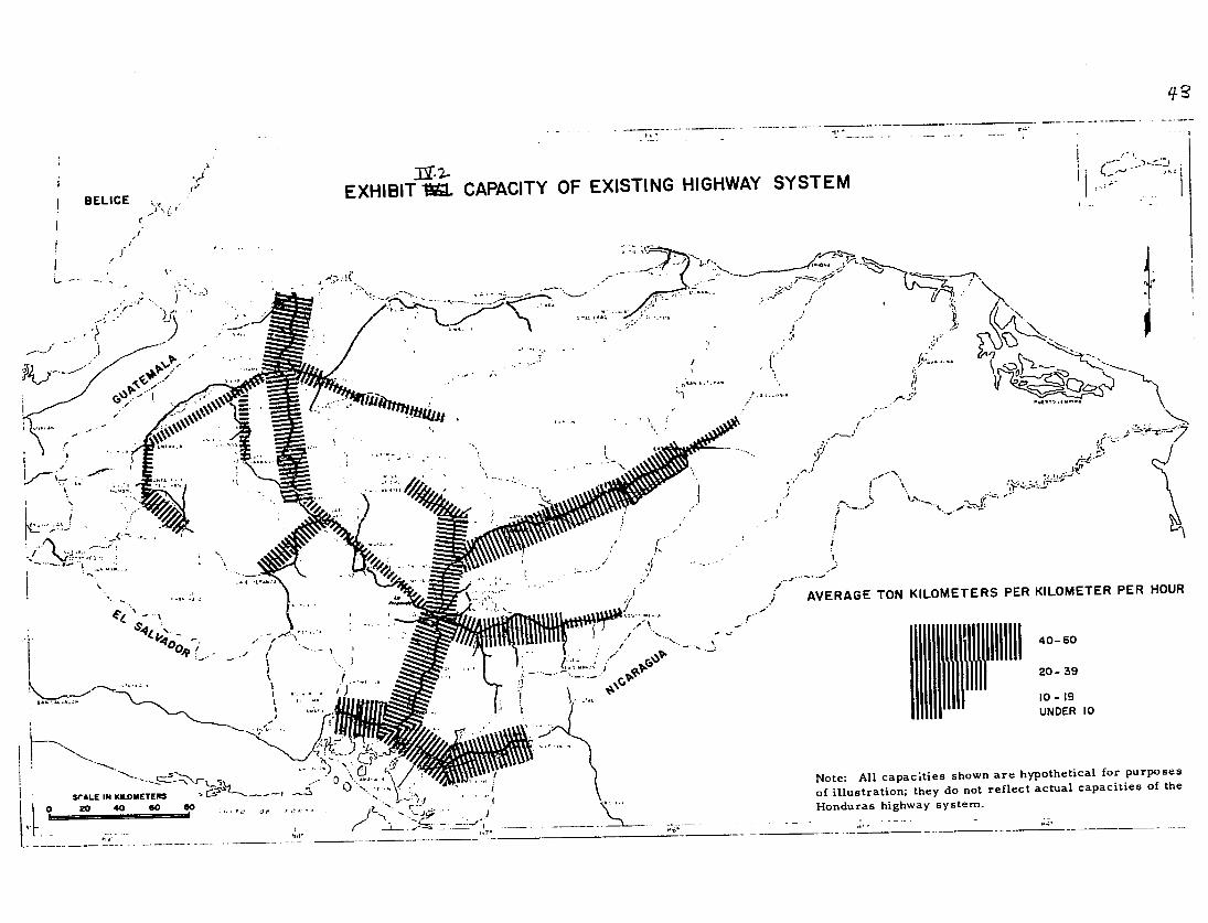
Including some average unit costs for each segment of the system (as dis
cussed in Chapter VI) directly on the map may sometimes be useful. Exhibit
IV.2 presents an example of a capacity mapping, and Exhibit IV.1 (which is a
reproduction of Exhibit 111.3), representing traffic movement, is overlaid on
transparent paper to facilitate comparison of capacity with demand.
Physical capacity of each element of the system will be defined sepa
rately for:
a. Rolling stock or vehicles.
Since rolling stock ordinarily moves from one to another part of the
system, the measure of capacity in this respect is meaningful only for the
whole system.' It refers to the total available capacity within the country
given the existing numbers and present efficiency of utilization. Increase
in capacity ma.y be accomplished by improving operational efficiency or by
increasing the number of units, either by manufactures or by imports from
abroad.
b. Fixed assets: highways, rail lines, ports, airports.
(i) Terminal, warehouses, marshalling yards, etc.
(ii) Line itself, i.e., the rail track, highway, pipeline,
or beltway.
TI
I .E L CE EXHIBIT M HIGHWAY FREIGHT MOVEMENTS CS,,
- LA C 0
I'
0I0•0 Go/o dO FcHo ,jH ndrauhgwaosstm 0-9
. ..
_ - 7 1 ....., ..... . - ..... .... ."r ... AVERAGE TON KILOMETERS PER KILOMETER PER HOUR
0 , o,,i., 'IUNDER
NI CA RA GU A
10
SCALE INKLMEE SCA~
.... INKiu"rTES,,... l"J
CAi.... ":" "'"°'" .....
Note: All volumes shown are hypothetical for purposes of illustration; they do not reflect actual volumes of the Honduras highway system.
0 Golf i0
880Fan-se 8do IsI
I I
-
-
EXHIBIT V CAPACITY OF EXISTING HIGHWAY SYSTEM BELICE
I ~~
44
I
.".-... ....
..........
..... ..... ...
.1:-
J -
......,.... .-- i i,'
.,-.
'....,;
S
.
LT
k?/.
40-60
- -':- K,.... .. "_"_... __ ._ ..
____.... IHIIIIIBII20-39 I 10-19
UNDER
__ _ __" _ _"__ __ __ __. _-
10
_-_ _ _ _ _\_,_
All capacities shown are hypothetical for purposes~I54 0Note: ~ illustration; they do not reflect actual capacities of the~ INKIWETEPS SrAL IN ILOMTERSof
0 . "0 Honduras highway system.__,__.__"_._._..... 60.,
44
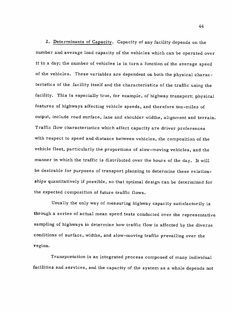
2. Determinants of Capacity. Capacity of any facility depends on the
number and average load capacity of the vehicles which can be operated over
it in a day; the number of vehicles is in turn a function of the average speed
of the vehicles. These variables are dependent on both the physical charac
teristics of the facility itself and the characteristics of the traffic using the
facility. This is especially true, for example, of highway transport; physical
features of highways affecting vehicle speeds, and therefore ton-miles of
output, include road surface, lane and shoulder widths, alignment and terrain.
Traffic flow characteristics which affect capacity are driver preferences
with respect to speed and distance between vehicles, the composition of the
vehicle fleet, particularly the proportions of slow-moving vehicles, and the
manner in which the traffic is distributed over the hours of the day. It will
be desirable for purposes of transport planning to determine these relation
ships quantitatively if possible, so that optimal design can be determined for
the expected composition of future traffic flows.
Usually the only way of measuring highway capacity satisfactorily is
through a series of actual mean speed tests conducted over the representative
sampling of highways to determine how traffic flow is affected by the diverse
conditions of surface, widths, and slow-moving traffic prevailing over the
region.
Transportation is an integrated process composed of many individual
facilities and services, and the capacity of the system as a whole depends not

45
only on the capacity of each element, but also on the synchronous functioning
of each element with every other. The functioning of a port is a clear
example of this. The components of the port operation may be grouped in
three classes: (1) navigational facilities, (2) cargo handling facilities including
berthing, and (3) auxiliary facilities including warehousing and inland transport
to and from the port. The capacity of the entire port complex will be limited
to the lowest common denominator, i.e., the lowest capacity of the individual
links. If cargo handling capacity is adequate, a more limited capacity to
transport the goods away from the port will result in overcrowding of ware
housing--this implies that the capacity of either warehousing or inland trans
port (or both) must be increased, depending on the relative costs in the parti
cular case.
Capacity assessment of any transport facility is a technical matter
which will ordinarily require the services of a qualified engineer. In some
cases, reliable information will be readily available, either in published form
or, upon inquiry, from engineering staffs of railways, port authorities, and
highway research stations. However, information thus obtained may reflect
only some aspired-for capacity, far removed from reality. This is particularly
true for highways where records of traffic movements are not normally
available, as opposed to railroads, ports, and pipelines where accounts of
traffic movements are customarily recorded. An attempt should be made to
verify all such capacity data by direct field surveys.

46
B. The Concept of Capacity and Its Role in Transport Planning
The concept of physical capacity does not by itself lend to the solution
of planning tasks. It is only when the physical variables are translated
into engineering or economic cost terms that they assume an operational
significance and can contribute to the investment planning process.
For any given facility of specified design standards, such as a high
way segment or a rail marshalling yard, as the volume of traffic grows
larger and larger a point will be reached at which average variable costs
(operating, maintenance, and inventory costs) / turn upward and increase
/ See Chapter VI below for a definition of the various cost components.
For some empirical information on the cost functions of different modes of
transport see Richard Heflebower, "Economic Characteristics of Transport
Modes," in Gary Fromm (ed.), Transport Investment and Economic Develop
ment (Brookings Institution: 1965).
with every successive unit of traffic as congestion increases. Obviously a
"trade-off" exists between the increasing variable costs of the congested
facility, on the one hand, and the capital costs for a base facility to higher
design stadnards (and therefore lower variable costs), on the other. The
engineering-economic task is to determine that particular level of capa
city or design standard--the optimal design capacity--which results in the

47
lowest average total unit cost for the volume of traffic which is expected
(taking into consideration, of course, all expected feedback effects of trans
port demand on supply).
The optimal design capacity for any specified volume of traffic will
depend not only on the physical characteristics of alternative facilities and
the flow characteristics of the traffic, but it will depend also on economic
factors--the opportunity values of foreign exchange, skilled and unskilled
labor, the opportunity rate of interest and the investment planning time
horizon. Because these factors will vary widely between countries, stan
dard charts which portray generally applicable design standards in such
high income countries as the United States will usually be entirely inappro
priate for the less-developed countries, and new standard guidelines must
be derived by detailed engineering and economic analyses. /
/ See Chapter VI.
Ouce these guidelines have been derived, the kind of capacity survey
described earlier in this chapter may be undertaken. This survey uses
these guidelines as substitutes or approximations to the more intensive
engineering-economic analyses. The survey serves to define the broad
outlines of the transport system and pinpoint potential trouble spots; it
provides a perspective on the relative importance of the various transport
problems which may arise. Once the outlines of the whole problem are

48
established, the detailed analyses described in Chapters VI and VII must
be implemented to determine the best solutions in each separate case. In
this way the capacity survey can contribute substantially to transport
planning. But it should never be taken as more than an approximation, an
overall reconnaissance method.

Required Information:
Techniques of Analysis:
Source:
EXHIBIT IV.3
SUMMARY: APPRAISAL OF PRESENT TRANSPORT CAPACITY
Economic-engineering determination of guidelines to capacities of alternative design specifications of different transport facilities.
Capacity mapping of each segment of existing transport system, separately for terminal and line facilities.
Tabulation of capacities of vehicle fleets.
Definition of any seasonality in use of facilities.
Engineering traffic flow/speed measurement experiments. Analysis of traffic flow statistics.
Economic -engineering analysis to determine optimal design capacities.
Previous studies by engineering staffs of railways, port authorities, highway research stations, pipeline companies.
Direct undertaking of traffic flow experiments.
Simple statistical analysis of traffic flow data where available. [May be useful, but not ordinarily adequate by itself.]
50
CHAPTER V
ESTIMATING BENEFITS FROM TRANSPORT INVESTMENTS
A. Real National Income as a Measure of Benefits
1. The "National Income Benefits Criterion"
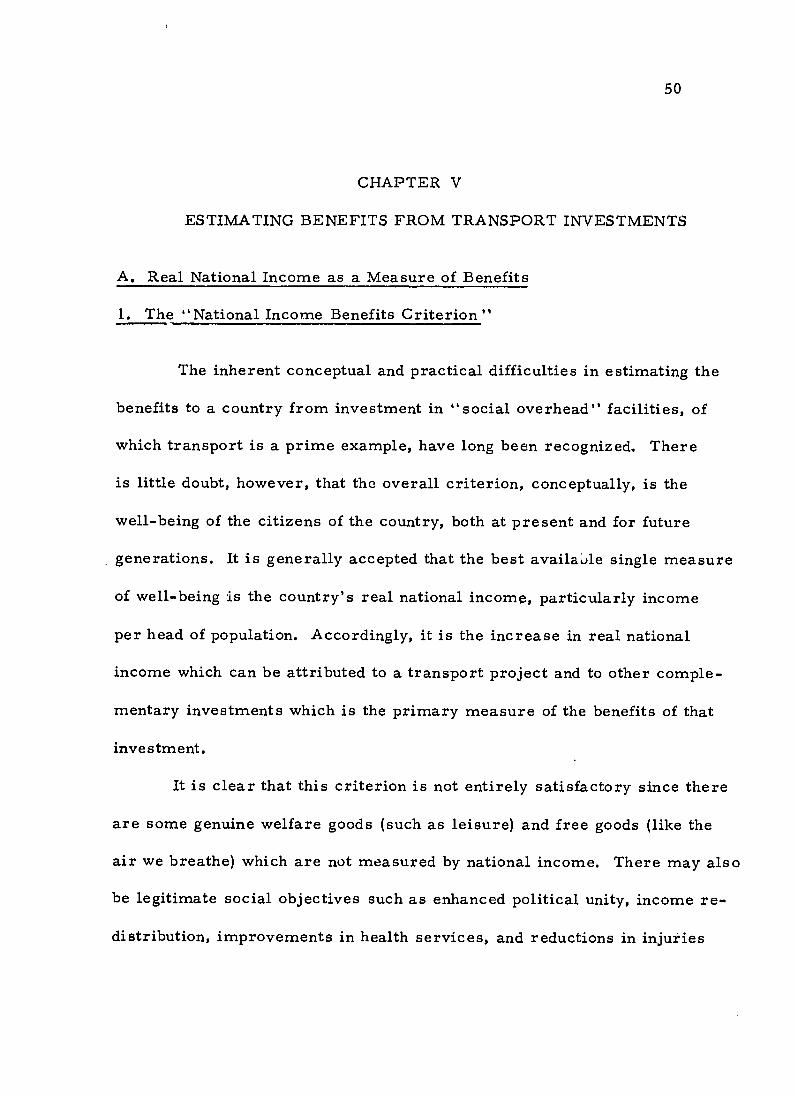
The inherent conceptual and practical difficulties in estimating the
benefits to a country from investment in "social overhead" facilities, of
which transport is a prime example, have long been recognized. There
is little doubt, however, that the overall criterion, conceptually, is the
well-being of the citizens of the country, both at present and for future
generations. It is generally accepted that the best availabile single measure
of well-being is the country's real national income, particularly income
per head of population. Accordingly, it is the increase in real national
income which can be attributed to a transport project and to other comple
mentary investments which is the primary measure of the benefits of that
investment.
It is clear that this criterion is not entirely satisfactory since there
are some genuine welfare goods (such as leisure) and free goods (like the
air we breathe) which are not measured by national income. There may also
be legitimate social objectives such as enhanced political unity, income re
distribution, improvements in health services, and reductions in injuries

51
and deaths due to accidents which are difficult to measure in money terms.
The division between present consumption and real savings and invest
ment, which determines the division of welfare between present and
future generations, may reflect a wealth and income distribution which the
public consensus, as reflected by the governmental decision process,
regards as unjust. A value judgment may be made that it is desirable to
sacrifice some increase in income in order to achieve a preferred distribu
tion of income between different groups of the society--or vice versa.
Because these noneconomic or intangible benefits cannot be
measured in the same terms as the other components of the problem,
there is no obvious criterion which can be used automatically to compare
different projects. However, this situation, which is common not only to
transportation but to nearly all public undertakings, is not entirely intrac
table. In general the analyst should:
(i) Make every attempt to determine that the proposed benefits
actually do exist, quantifying these in money or physical units where
possible. Increased accessibility to medical care and eradication of
disease are real benefits. Political unity can be rather more elusive and
imaginary, but e.. 7blishing law and order, or putting down insurgents in
remote areas can be very real and confirmed to be so.
(ii) Determine the costs of alternative means to achieve the same
kinds of objectives. The costs to achieve these objectives through alterna
tive means can be used as one index of their value.

52
(iii) Where no other procedure is evident, the intangible benefits of
each project alternative can be described in as specific terms as possible
alongside the computation of quantifiable costs and benefits. Broad allusions
to improved economic efficiency or enhanced political unity are, without
substantiation, worthless characterizations.
When noneconomic benefits are portrayed in this way, it is always
possible to compare the economic costs with the proposed benefits and the
decision-maker is in a position to make a judgment on the preferable trade
offs between the economic and noneconomic costs and benefits of alternative
proposals.
In summary, it is the expected increase in real national income which
can be attributed to the investment which constitutes the primary measure of
benefits. In addition, any important noneconomic (intangible) effects--good or
bad--should be described in as specific terms as possible. This, then, is
the national income benefits criterion which is proposed here. In the next
section some alternative measures are evaluated in terms of this criterion,
and in section B following, application of the criterion is discussed.
2. Comparison of National Income Criterion With Costs and Savings and Land
Value Measures
The national income criterion proposed above, even with all its own
conceptual weaknesses, may still represent a relatively high ideal when
53
compared to the time, data, and other limiting circumstances of the practical
planning situation. _/ In this context, one possible approach might be to
_/ But the practical difficulties of using a national income approach can be
exaggerated. Consider the techniques proposed in Section V.B following.
break down the increase in national income into components which could be
more readily observed and measured. This is, of course, in fact the way
that the problem has traditionally been approached, although not without loss
of simplicity which has resulted in a great deal of confusion. Exhibit V.1
presents a comparison and synthesis of four possible approaches.
Measure A is the national income criterion, minus intangibles, which
was discussed above and is developed further below. Measures B, C, and D,
whose components represent commonly used measures of benefits, are
defined so that they are conceptually equivalent to each other and to the in
crease in national income, measure A. Comparison of these measures in
this format makes clear why partial measures such as transport cost savings,
shippers savings and/or land values can so easily be misrepresented as
estimates of the benefits of transport investments. These measures may
eitherignore various effects, such as elements (4), (5), and (6) and sometimes (3)of
Exhibit*V. 1, which would tend to understate the actual increase in natidnal income. Or
they may add together two or more elements, which reflect one and the same
benefit, and thus nverstate the increase in income. For example, it has not

54
EXHIBIT V. 1
Comparison of National Income Measure and Other Measures of Benefits
[All measures are equivalent: Measure A = 'Measure B = Measure C Measure D, and each Measure is composed of separate elements numbered (1), (2), etc.]
Measure A (1) Increase in national income due National Income to investment in transport and Approach complementary activities.
Measure B (2) Transport Cost Savings on Cost Savings Present Traffic Approach
plus
Increase or decrease in economic efficiency of resources which are employed:
(3) Near the transport facility, and (4) Elsewhere in the economy
plus
Employment of formerly idle resources in areas:
(5) Adjacent to transport facility, and,
(6) Elsewhere in the economy
Measure C (7) Increased profits to transport Shippers Savings carriers Approach
plus
(8) Savings to shippers located near the transport facility
plus
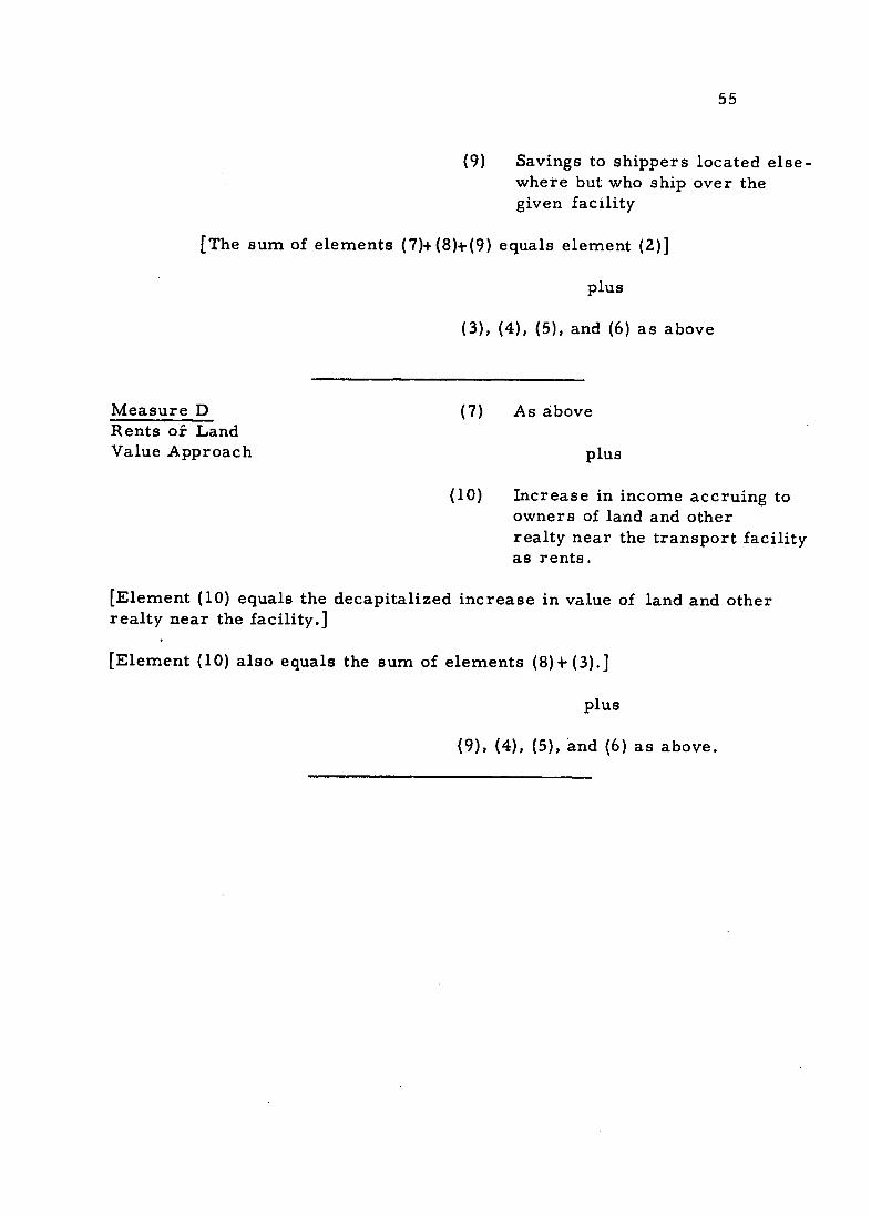
55
(9) Savings to shippers located elsewhere but who ship over the given facility
[The sum of elements (7)+(8)+(9) equals element (2)]
plus
(3), (4), (5), and (6) as above
Measure D (7) As above Rents oi Land Value Approach plus
(10) Increase in income accruing to owners of land and other realty near the transport facility as rents.
[Element (10) equals the decapitalized increase in value of land and other realty near the facility.]
[Element (10) also equals the sum of elements (8)+ (3).]
plus
(9), (4), (5), and (6) as above.

56
been unusual to observe either cost savings (2) or (8) added to (10), the in
crease in land rents which reflect the reduction in transport costs. To use
such a measure represents double counting of actual benefits. A review of
current practices indicates that estimates of benefits of proposed transport
investments in the underdeveloped countries have in several cases overstated
benefits which were ultimately realized. /
/ Overestimation of benefits has been due not only to the type of double
counting error described above, but also to overoptimistic assumptions with
respect to the rate of growth of traffic (see Section II.B above) and, in some
cases, overestimates of savings in operating costs.
3. Advantages and Disadvantages of the National Income Measure
Exhibit V.1 also makes evident some of the advantages and difficulties
of the national income approach. It is difficult to obtain any meaningful
measure of elements (4) and (6). There is commonly no way of isolating an
increase in income from a more effective utilization of resources elsewhere
in the economy which in turn results from a particular transport development.
However, these effects may be of some importance to the investment decision.
There may be no alternative but to leave them as "intangibles" and to note
that the estimate may understate benefits by this (uncertain) amount.
However, element (2), operating cost savings--the measure most often
seen because it is relatively easy to estimate--is inadequate as the single

57
measure of benefits. It excludes what may often be the most important effect:
the increase in efficiency of presently employed resources and new employ
ment of formerly idle resources in the area most directly served by the
transport facility. This brings into focus one major factor which must always
be taken into consideration before estimating the ultimate benefits of an
investment: the form which transport cost savings will take.
Even though an investment may result in a substantial reduction of
transport costs, the impact of these cost savings on the economy may either
be quite important or of little significance.
The greater the amount of the savring through reduced charges to shippers
and the greater the elasticity of supply, the greater will be the response of
the economy in increased output, employment, and income. However, if all
the transport cost reductions serve merely to increase the carriers' profits
and there are no reductions in the rates charged shippers, the beneficial effect
of the investment on the economy may be minimal. On the other hand,
experience has shown that transport operators, particularly small trucking
firms, can be very enterprising in using the increased profits which result
from public transport investments. In some cases they have financed new
equipment, improved service, and other productive investments from increased
profits. Where this occurs, transport cost savings become the source of
sizeable new investments. Perhaps even more important, they create the

58
opportunity for developing a new rational, profit-seeking, and risk-taking
entrepreneurial group which is one of the most effective catalysts of economic
development.
An important advantage of the national income approach is that, in
computing this measure (as described later), it is virtually impossible to
overlook complementary investments. Associated facilities, such as housing,
irrigation, fertilizers, and other private industry, are often necessary if any
transport project is to increase national income. This is especially true for
penetration or development roads in rural areas. In appraising an undertaking
the total necessary investments must be included in costs and the whole
package compared with expected benefits.
These effects are emphasized in the national income approach and can
for the most part be predicted using the simple techniques outlined in the
section immediately following.
B. Application of the National Income Measure of Benefits
1. Definition of the Economic Region Affected by the Proposed Investment
For national transport planning, obviously the whole country is the
appropriate economic region. But for studies at the project level, a smaller,
more manageable economic region--perhaps an economic corridor, or a river
basin--will ordinarily contain the major impact of the proposed transport
improvements.
59
The area affected by a single transport project depends on both the
size of the transport cost reduction and service improvement and the sensiti
vity of output (or elasticity of supply) to cost reductions. In any case, both
of these components, unit cost savings and supply elasticities, must be computed
to determine projections of future output as described earlier in Chapter III.B.
In practice, the economist can determine geographic boundaries beyond which
the effect on output of a given project is so small that its computation is not
worth the cost to the study.
Even for very similar investment proposals, the nature and size of a
region which is appropriate for one case may be quite different from that which
is appropriate for another in a different region or country. For example, the
important effects of constructing one rural road segment may be contained
within an area ten miles on either side of the road, and the effects of another
road built to the same design standards in another region may influence econo
mic activity fifty miles away. Determining the "zone of influence" of
proposed transport improvements is a matter for expert economic consideration
in each case.
2. Projections of the Increase in National Income Which Would Result From
Transport and Complementary Investments
The basic method in estimating benefits is to make two output projec
tions: what output in an economic region would be without the proposed
transport investment and what it would be if the investment were made. The
60
difference between the two estimates is taken to represent the benefit which
is attributable to transport and its complementary investments.
a. Projections of Gross Physical Outputs. The expert economic
analysis of the area affected by the transport investment (described in
Chapters II.B and iII.B) will determine the probable increase in output of all
major products, taking into consideration the feedback effects of the proposed
investment. The analysis is based on a survey of: (1) physical productive
potential, (2) market potential, and (3) investment plans of government and
private industry. If the engineer or transport specialist can specify the loca
tion and expected haulage costs for each proposed transport facility, then the
agriculture, mineral, forestry, and industry experts estimate (at leastcan
within a range) the change in output of each commodity which could be expected
to result from that particular investment. These calculations are identical
with those described earlier in the derivation of traffic projections. (Chapter
III, pp. 33 ff.)
b. Pricing of Projected Outputs. Projected gross outputs of most industries
should be valued at their known or estimated wholesale price at the site of the
farm or plant. This is true of such industries as agriculture, fishing,
forestry, mining, manufacturing, and construction. /
_/ Net output in the transport and trade sectors will ordinarily be determined
not by gross output minus inputs but by direct estimates of depreciation and
factor payments to wages, interest, and rent.

61
Generally, the following principles should be adhered to in adjusting
for price distortions and changes:
(i) Increases in output for export or import substitution should be
valued at the true opportunity cost of foreign exchange, not at realized market
price after taxes. (See Chapter VI, p. 88 below.)
(ii) Changes in foreign prices of imports and exports affect the real
purchasing power of the country's foreign exchange earnings and are a major
determinant of the physical volume of trade. Therefore, it is of great impor
tance that the future course of foreign trade prices be projected as accurately
as possible, and the effects of fluctuations in prices should not be statistically
eliminated. (Because of the great uncertainty of future terms of trade, it will
often be useful to assume a range of possible trends.)
(iii) Equiproportionate changes in the overall domestic prices resulting
from purely monetary inflation or deflation should not affect the investment
decision and should be statistically eliminated by valuing future output at con
stant prices. Decreases in the cost of transportation and of goods which utilize
transport as a result of the proposed investment reflect real benefits to the
economy and should be taken into account by valuing future output at prices
constant at the initial level. /
_/ But changes in the relative prices of inputs affect resource allocation and
should not be eliminated. Current, not constant, prices should be incorporated
in both the economic and financial analysis in this case. See Chapter VI, p. 91.

62
3. Determining Income: Netting out Purchases from Other Sectors and
Regions
The increase in national income for the economy as a whole does not
equal the total or gross increase in the value of production as determined
above since much of the reported increase may simply reflect purchases from
other industries, both within and without the region affected. For example,
gross sales of the food processing industry reflect purchases which have al
ready been included in the gross output of agriculture. There are two basic
methods of netting out purchases of intermediate inputs from gross outputs to
arrive at the net output, value-added, or net income originating in wages,
profits, interest, and rent which can be attributed to each economic sector. _
_/ Refer to any standard treatise on national income (or social) accounting,
such as Paul Studenski, The Income of Nations (New York University Pressi
1958, part II, especially Chapters 17 and 18. Walter Isard (ed.), Methods of
Regional Analysis (The Massachusetts Institute of Technology Pressj 1960),
provides an introductory discussion and a useful bibliography on both national
and regional income accounting in Chapter 4.
The first is directly subtracting EL11 purchases from other sectors from the
gross output of each sector--when this information is available or can be
estimated. The second is multiplying the gross output of each sector by a
63
separately determined percentage which represents the average net value added
in that industry.
Because this is a regional, rather than a national, accounting frame
work, it is necessary to make a second adjustment to account for the loss of
output incurred elsewhere in the economy by the shift of labor and capital
resources to the region affected by the proposed investment. This means
deducting the costs of these resources in their alternative employments. It
is difficult to determine what part of the total increase in resources employed
has actually shifted from outside the region and what part was formerly un
employed and represents no net loss. This is a matter which can be approached
only by expert economic analysis, and even then an approximation may be the
best that can be hoped for, depending upon the individual case.
Thus we have two alternative
sectors or industries:
Deductible Costs Method
Net income adjusted for interregional resource flows.
Percentage-Value-Added Method
Net income adjusted for interregional resource flows.
measures for net income by economic
= Gross output minus purchase of intermediate goods minus wages, profits, interest of resources, shifted into the region from productive employments outside the region.
= (Gross output) x (percentage value added in this sector)
minus wages, profits, interest of resources shifted into the region from productive employments outside the region.
64
Finally, the total benefit of the transport and complementary invest
ments is given by summing the net value added (adjusted for interregional
resource flows) for each sector, to arrive at the increase in national income.
Increase in national income = Sum of increase in net value attributed to investments, added for each sector (adjusted
for interregional shifts of resources) attributed to investments.
C. Examples of Actual Application of National Income Measure
Lest the reader be overwhelmed by real and imagined difficulties in
the income estimation problem, two case studies which actually employed a
national income criterion are presented in some detail here. Because these
are case studies of previous investment decisions, they enjoy the advantage of
hindsight. This eliminates predictions from the problem of estimating the in
crease in national income. However, all other of the problems which face
planners in determining and valuing physical output within the data limitations
of the underdeveloped countries are clearly evident. These examples are
presented not as ideal standards but as heroic attempts to implement a new
methodology within very severe circumstances. The authors of this study
contend that the approach used in these cases, despite the obviously great
limitations, represents a far superior measure of the benefits from invest
ment in transport and ancillary facilities than any of the traditional measures.

65
Example 1: Computing Increase in National Income by Deductible-Cost Method: El Salvador's Littoral Highway _I
_/ This example is largely taken from Leon V. Hirsch, "The Littoral Highway
in El Salvador" (The Brookings Institution, forthcoming). However, some
changes in concept have been introduced to conform with terminology used
here, and the reader should consider the data presented as illustrative only.
MEASUREMENT: IDEAL AND POSSIBLE
Ideally, to measure the agricultural changes that have taken place after the building of the Littoral Highway, present cultivated area and output should be compared with an estimate of what would probably have been the case had the road not been constructed.
Estimating Increase in Gross Agricultural
Output Due to Highway
Available data Unfortunately, no comparative agricultural data by municipalities are presently available. Eventually, figures for the 1961 agricultural census will be obtained and these can be compared with those of the 1950 census. Even if these figures were presently available they would leave something to be desired, since early segments of the road were not completed until 1958, and the final segment until 1962. There was probably a delay in response to the road and therefore the 1961 census would not have recorded all of the effects of the road even in areas where it had been completed.
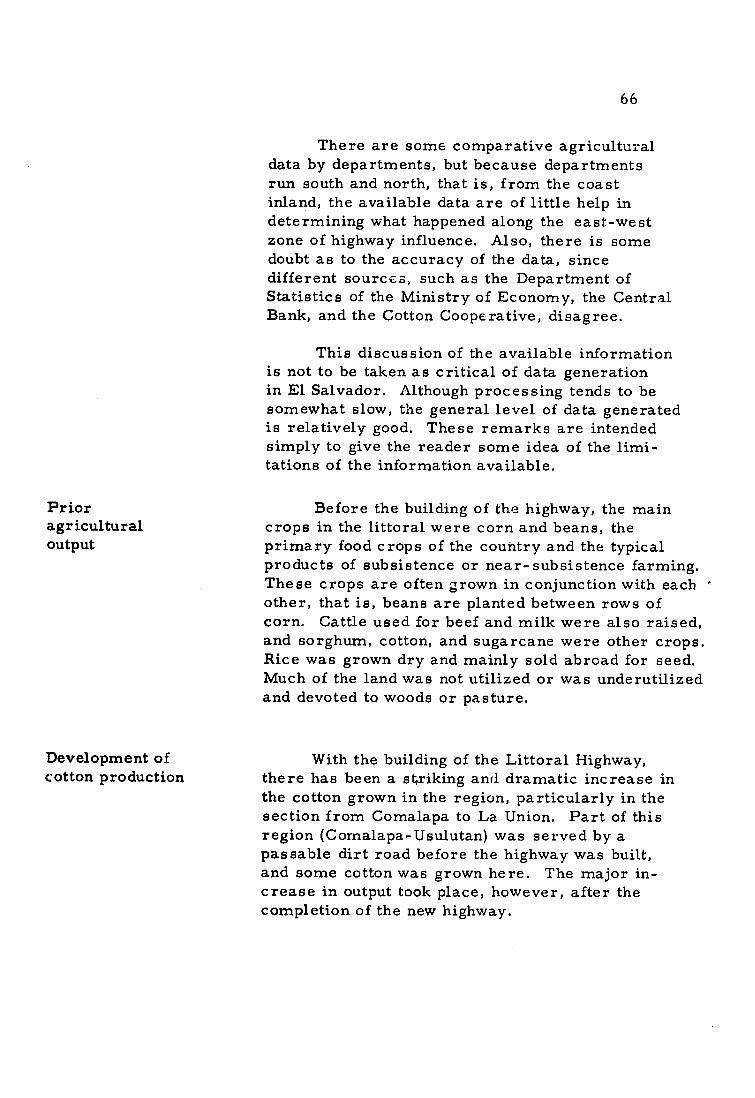
Prior agricultural output
Development of cotton production
66
There are some comparative agricultural data by departments, but because departments run south and north, that is, from the coast inland, the available data are of little help in determining what happened along the east-west zone of highway influence. Also, there is some doubt as to the accuracy of the data, since different sources, such as the Department of Statistics of the Ministry of Economy, the Central Bank, and the Cotton Cooperative, disagree.
This discussion of the available information is not to be taken as critical of data generation in El Salvador. Although processing tends to be somewhat slow, the general level of data generated is relatively good. These remarks are intended simply to give the reader some idea of the limitations of the information available.
Before the building of the highway, the main crops in the littoral were corn and beans, the primary food crops of the country and the typical products of subsistence or near-subsistence farming. These crops are often grown in conjunction with each other, that is, beans are planted between rows of corn. Cattle used for beef and milk were also raised, and sorghum, cotton, and sugarcane were other crops. Rice was grown dry and mainly sold abroad for seed. Much of the land was not utilized or was underutilized and devoted to woods or pasture.
With the building of the Littoral Highway, there has been a striking and dramatic increase in the cotton grown in the region, particularly in the section from Comalapa to La Union. Part of this region (Comalapa-Usulutan) was served by a passable dirt road before the highway was built, and some cotton was grown here. The major increase in output took place, however, after the completion of the new highway.
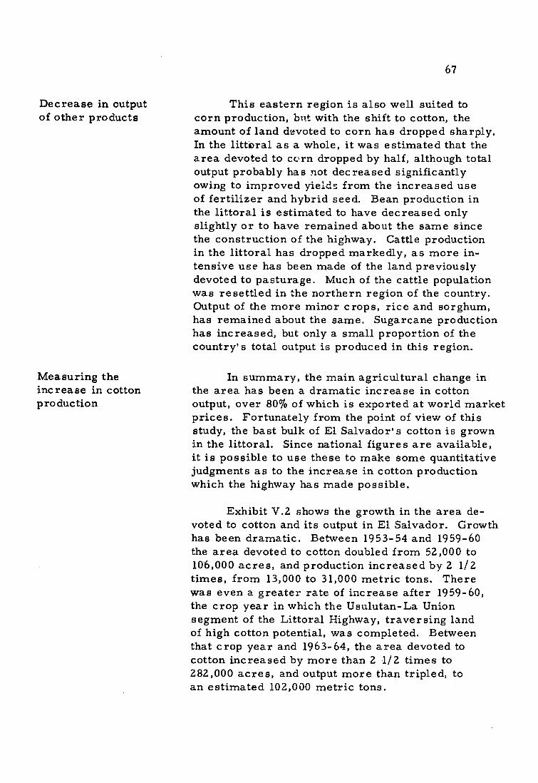
67
Decrease in output of other products
Measuring the increase in cotton production
This eastern region is also well suited to corn production, bit with the shift to cotton, the amount of land devoted to corn has dropped sharply. In the littoral as a whole, it was estimated that the area devoted to cc.,rn dropped by half, although total output probably has not decreased significantly owing to improved yields from the increased use of fertilizer and hybrid seed. Bean production in the littoral is estimated to have decreased only slightly or to have remained about the same since the construction of the highway. Cattle production in the littoral has dropped markedly, as more intensive use has been made of the land previously devoted to pasturage. Much of the cattle population was resettled in the northern region of the country. Output of the more minor crops, rice and sorghum, has remained about the same. Sugarcane production has increased, but only a small proportion of the country's total output is produced in this region.
In summary, the main agricultural change in the area has been a dramatic increase in cotton output, over 80% of which is exported at world market prices. Fortunately from the point of view of this study, the bast bulk of El Salvador's cotton is grown in the littoral. Since national figures are available, it is possible to use these to make some quantitative judgments as to the increase in cotton production which the highway has made possible.
Exhibit V.2 shows the growth in the area devoted to cotton and its output in El Salvador. Growth has been dramatic. Between 1953-54 and 1959-60 the area devoted to cotton doubled from 52,000 to 106,000 acres, and production increased by 2 1/2 times, from 13,000 to 31,000 metric tons. There was even a greater rate of increase after 1959-60, the crop year in which the Usulutan-La Union segment of the Littoral Highway, traversing land of high cotton potential, was completed. Between that crop year and 1963-64, the area devoted to cotton increased by more than 2 1/2 times to 282,000 acres, and output more than tripled, to an estimated 102,000 metric tons.

68
EXHIBIT V.2. El Salvador Cotton Production, Area, Quantity, and Price, 1953-54 to 1963-64
Area Quantity of Lint Average Price (thousands (thousands of (U. S. dollars
Crop Year of acres) metric tons) per metric ton)
1953-54 52.2 12.9 761.9 1954-55 73.1 20.5 734.1 1955-56 113.0 30.8 634.2 1956-57 94.8 32.4 617.5 1957-58 98.7 36.0 593.0 1958-59 132..4 39.7 517.9 1959-60 106.3 31.1 571.9 1960-61 140.1 41.9 584.3 1961-62 202.5 58.7 585.7 1962-63 231.4 72.4 584.3 1963-64 282.1 101.9 (est.) N.A.
Source: Salvadorean Cotton Cooperative, Ltd., Memoria for 1962-63 harvest. (1963-64 data, Ministry of Agriculture and Cattle.)
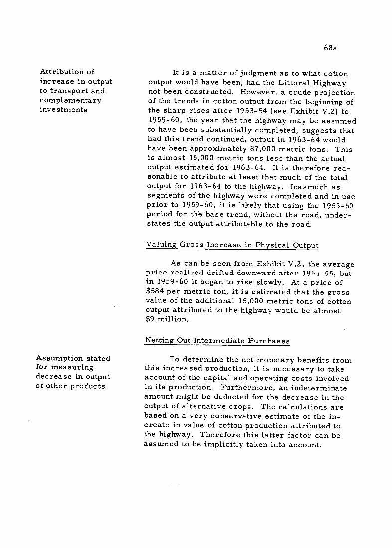
Attribution of increase in output to transport and complementary investments
Assumption stated for measuring decrease in output of other prod-ucts
68a
It is a matter of judgment as to what cotton output would have been, had the Littoral Highway not been constructed. However, a crude projection of the trends in cotton output from the beginning of the sharp rises after 1953-54 (see Exhibit V.2) to 1959-60, the year that the highway may be assumed to have been substantially completed, suggests that had this trend continued, output in 1963-64 would have been approximately 87,000 metric tons. This is almost 15,000 metric tons less than the actual output estimated for 1963-64. It is therefore reasonable to attribute at least that much of the total output for 1963-64 to the highway. Inasmuch as segments of the highway were completed and in use prior to 1959-60, it is likely that using the 1953-60 period for the base trend, without the road, understates the output attributable to the road.
Valuing Gross Increase in Physical Output
As can be seen from Exhibit V.2, the average price realized drifted downward after 1954-55, but in 1959-60 it began to rise slowly. At a price of $584 per metric ton, it is estimated that the gross value of the additional 15,000 metric tons of cotton output attributed to the highway would be almost $9 million.
Netting Out Intermediate Purchases
To determine the net monetary benefits from this increased production, it is necessary to take account of the capital and operating costs involved in its production. Furthermore, an indeterminate amount might be deducted. for the decrease in the output of alternative crops. The calculations are based on a very conservative estimate of the increate in value of cotton production attributed to the highway. Therefore this latter factor can be assumed to be implicitly taken into account.
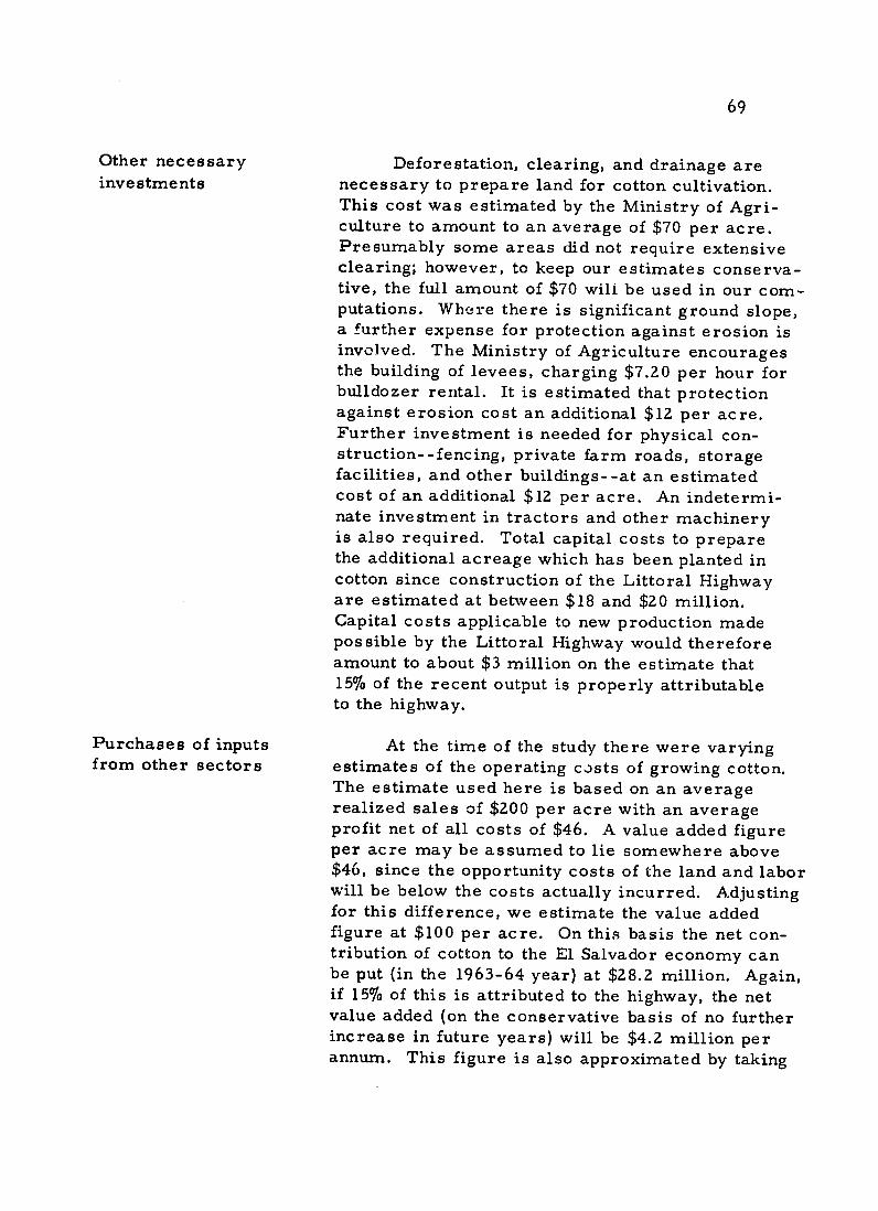
69
Other necessary investments
Purchases of inputs from other sectors
Deforestation, clearing, and drainage are necessary to prepare land for cotton cultivation. This cost was estimated by the Ministry of Agriculture to amount to an average of $70 per acre. Presumably some areas did not require extensive clearing; however, to keep our estimates conservative, the full amount of $70 wili be used in our computations. Where there is significant ground slope, a further expense for protection against erosion is involved. The Ministry of Agriculture encourages the building of levees, charging $7.20 per hour for bulldozer rental. It is estimated that protection against erosion cost an additional $12 per acre. Further investment is needed for physical construction- -fencing, private farm roads, storage facilities, and other buildings--at an estimated cost of an additional $12 per acre. An indeterminate investment in tractors and other machinery is also required. Total capital costs to prepare the additional acreage which has been planted in cotton since construction of the Littoral Highway are estimated at between $18 and $20 million. Capital costs applicable to new production made possible by the Littoral Highway would therefore amount to about $3 million on the estimate that 15% of the recent output is properly attributable to the highway.
At the time of the study there were varying estimates of the operating costs of growing cotton. The estimate used here is based on an average realized sales of $200 per acre with an average profit net of all costs of $46. A value added figure per acre may be assumed to lie somewhere above $46, since the opportunity costs of the land and labor will be below the costs actually incurred. Adjusting for this difference, we estimate the value added figure at $100 per acre. On this basis the net contribution of cotton to the El Salvador economy can be put (in the 1963-64 year) at $28.2 million. Again, if 15%o of this is attributed to the highway, the net value added (on the conservative basis of no further increase in future years) will be $4.2 million per annum. This figure is also approximated by taking

70
half of the gross value ($9 million) of the output attributed to the road in the preceding calculations.
Example 2: Computing Increase in National Income by Percentage-Value-Added Method: The Cochabamba-Santa Cruz Highway /
/ This example is taken from the forthcoming study by Barbara Berman,
"Transportation in the Strategy of Bolivian Development: The Cochabamba-
Santa Cruz Highway:"(The Brookings Institution, forthcoming).
-Agricultural Production
The principal result of the cheaper linkage and other facilities has been the expansion of agricultural production documented in Exhibits V.3 and V.4. Bolivia is now, or will soon be, self-sufficient in sugar and rice, and the Santa Cruz area accounts for all but a small proportion of the country's production of these two products. Sugar, for which we have the most complete time series, increased tenfold in physical volume of production between 1954, the year the Cochabamba-Santa Cruz Highway was open to traffic, and i962. In 1962, domestic production accounted for 83 percent of consumption. Rice production is said to have tripled between 1958 and 1963. Production of rice in 1962 about equalled what national consumption was estimated to be in 1958. /
/ Maldonado San Martin, Gonzalo, The General Agricultural Marketing Report of Bolivia, Servicio Agricola Interamericano (Bolivian government agency), La Paz, 1959.
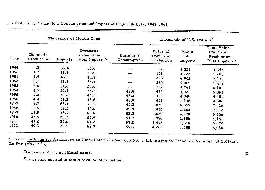
EXHIBIT V.3. Production, Consumption and Import of Sugar, Bolivia, 1949-1962
Thousands of Metric Tons Thousands of U.S. Dollarsa
Total ValueDomestic Value of Value DomesticDomestic Production Estimated Domestic of Production
Year Production Imports Plus Importsb Consumption Production Imports Plus Importsb
1949 .2 33.4 33.6 -- 32 4,321 4,3531950 1.2 36.8 37.9 -- 161 5,122 5,2831951 1.5 43.5 44.9 -- 233 6,905 7,1381952 2.3 33.1 35.4 -- 350 5,069 5,4191953 3.0 51.6 54.6 -- 332 5,768 6,1001954 4.5 50.1 54.5 47.8 439 4,925 5,3641955 4.3 42.8 47.1 48.3 409 4,046 4,4541956 4.4 41.2 45.6 48.8 447 4,148 4,5961957 8.7 66.7 75.5 49.3 859 6,557 7,4161958 15.5 33.5 49.0 49.9 1,550 3,362 4,9121959 17.5 46.1 63.6 52.3 1,629 4,278 5,9061960 24.5 26.5 50.9 54.7 1,996 2,156 4,1511961 41.2 20.0 61.2 57.2 3,412 1,658 5,0701962 49.2 20.5 69.7 59.6 4,205 1,755 5,960
Source: La Industria Azucarera en 1962, Boletin Ec6nomico No. 4, Ministerio de Economia Nacional (of Bolivia), La Paz (May 1963).
aCurrent dollars at official rates.
bRows may not add to totals because of rounding.

72
EXHIBIT V.4. Estimated Rice Production in Bolivia, 1958-1963 (Thousands of metric tons)
Year Amount
1958 12.5
1959 19.5
1960 23.3
1961 24.0
1962 24.0
1963 36.0
Source: Ministerio de Agricultura (of Bolivia), quoted in Economic and Program Statistics (U.S. Agency for International Development/Bolivia,
October 1963).

73
Estimating Gross Output Value
The first step in a numerical estimate of the current flow of benefits is an attempt at arriving at the Gross Regional Product (GRP) of Santa Cruz, as shown in Exhibit V.5. Column (1) of that exhibit gives estimates of the value of production by sector. Some estimates were arrived at by collating published data on local production by type for those categories in which data are available. Other items were estimated by taking percentages of national totals, and some are rather sketchily based on transportation records. One source of error in the estimate is that no allowance is made for products produced and consumed by farmers without recourse to the market place. On the other hand, "other activities" includes commerce, and was estimated to be the same proportion of national activities as the region's population to national population. This category may be overestimated because the capital city, La Paz, probably has much more than its share of the national product.
Netting Out Inputs From Other Sectors and Regions
Since Santa Cruz industries buy goods both from each other and from outside the Department, the values in column (1) include double counting of local productive activity and also include productive activity taking place elsewhere. Hence there is a downward adjustment in the numbers of column (1) made by applying the ratios in column (2) to get an estimate for each sector's contribution to GRP in column (3). The ratios were derived from the 1958 input-output table for Bolivia. The final sum for the 1962 estimate of Santa Cruz Gross Regional Product is $24 million, about 6 percent of Bolivia's Gross National Product.

--
--
EXHIBIT V. 5. Annual Gross Regional Product, and Portion Attributable to the Highway and Other Investments, Santa Cruz Department, 1962 (In millions of current U.S. dollars),
Sector
Sugar Rice Timber
Alcohol Cotton
Other agricultural products
Interurban road transport
Petroleum Other Activities
Physical Volume
49,000 metric tons c
24,000 metric tons d
4,329 thousand board feete
6 million litresc 3,000 metric tonsg
11,000 round trips of. 7,000 ton-kms. each
500 million litresk
(1)
Value of Pro-duction
4.2 c
3.8
.3f 1.0
1 . 5 h
i.0 j
1.9 i
6.01
8 . 0 m
(2)
Value Added per Dollar of Productiona
.85
.85
.85
.85
.85
.85
.66 1.00
.80
(3)
Value Added (GRP)
3.6 3.2
.3
.9 1.3
.8
1.3 6.0 6.4
23.8
(4)
Approximate Value Added Attributable to the
Highway and Other Non-Petroleum Investmentsb
3.2 2.8
.2
.7 1.0
.7
1.2
3.2
13.0
aDerived from the ratio of value added to production shown for 1958 by Planeamiento, 1961, Table 6,
except for petroleum.
bSee text for explanation.
CLa Industria Azucarera en 1962.

75
Footnotes to Exhibit V.5 continued
dPublications giving (conflicting) production estimates include
"Estadisticas Agropecuarias," Ministerio de Agricultura, La Paz, 1962, Datos Estadisticos Del Departamento De Santa Cruz, Oficina de Programas, USAID, La Paz, 1962 (mimeo.), and a CBF memorandum, Influenzia del Camino Cochabamba-Santa Cruz en El Desarrollo Del Pais. The latter also gives a price estimate as do SAI reports, from which Santa Cruz prices have been extracted.
eFrom a tabulation for 1961 made by the Director Forestal for TAMS,
reported in Eric D. Dodge, Preliminary Summary of Bolivian Economy and Transportation, Cochabamba, 1962.
f CBF, op. cit.
gIbid.
hprice on United States markets used in estimation.
iEstimated from data in Barbara R. Berman, Transportation In The Strategy of Bolivian Development: The Cochabamba-Santa Cruz Highway, (The Brookings Institution, forthcoming), Tables 4 and 6.
JEstimated by the author on the basis that about 15 percent of the trucks leaving Santa Cruz for Cochabamba carrying food and raw materials carry cargo in this category. (See Ibid., Table 4.)
kUSAID, "Recent Trends in the Bolivian Economy," (mimeo, undated).
1Estimated by applying to the estimated value of refined petroleum a multiplier equal to the proportion of value added by the petroleum industry attributable to crude production in the United States.
mThe city of Santa Cruz has about 9 percent of the nonrural population
of Bolivia. This figure is derived from taking 9 percent of Bolivian value added, exclusive of agriculture, mining, petroleum, and manufacturing.

76
Allowing for resources shifted from employments elsewhere in the economy
What part of this $24 million gross increase can be considered a net benefit from the national viewpoint? From the income side of the ledger, GRP, or value added, can be broken down into wages, profits, and depreciation._/
/ For purposes of this discussion other shares such as interest, rent, and so on are neglected.
It is a fair assumption that wage payments in Santa Cruz did not replace wage payments which would have been made in other areas of the economy, had the Santa Cruz developments not occurred. This does not mean that the men working in Santa Cruz are assumed to have been unproductive in their previous occupations, but rather that their place was taken by others who were formerly much less productive or non-productive, so that little output was lost on this account. A similar assumption can be made concerning profit, considered as a reward to entrepreneurs. Depreciation assumes that a capital good could produce value equal to its depreciation in any Bolivian region, and therefore an estimate of depreciation is subtracted. Another way of thinking about depreciation is to consider that the wearing away of (imported) capital is a flow import from outside the Santa Cruz economy, and that this stream of imports should be subtracted for the same reason that imported raw materials would be.
It might be argued that such items in the income account as "interurban" transport should show up as a cost rather than as a benefit, but to argue in this way would be to go against the logic of income accounting. The products which are transported include in their value the cost of that transport, but their production, transport, and final purchase means that the benefit derived from them can cover production and transport.

77
Annual maintenance
costs treated as a negative benefit
Attribution of
increase in income to transport and complementary investments
The nonlabor part of the cost of upkeep on the Cochabamba-Santa Cruz highway should be entered as a negative item in our benefit account. Total annual maintenance costs are estimated at $333 thousand per year,_/ once past neglect has been
/ Republica de Bolivia Junta Nacional de Planeamiento, Programa Preliminar de Transportes (1963), Table 237.
made good. Nonlabor costs of maintenance are estimated at 14 percent. / These maintenance
/ Ibid., Table 158.
expenditures are assumed to be sufficient to insure perpetual life to the highway.
Not all of the production in the Santa Cruz area is attributable to the highway and associated investments, so some of it must be subtracted to arrive at the gross benefits of the highway. In column (4) the amount of productive activity attributable to the effect of the highway and other investments has been estimated on a somewhat arbitrary basis. For example, none of the value added in petroleun has been included, on the ground that this activity would have occurred without the highway. Similarly, about half of the residual category "other activities" (mainly services of all sorts rendered by the urban population) has been excluded.
These calculations are summarized in Exhibit V.6. The net benefits. which we have calculated as currently running at $11.3-$11.8 million per annum cover benefit categories both (1) and (2) above, since no loss of prodv :tion in other regions has been assumed.

78
EXHIBIT V.6. Capital Costs and Current Flow of Benefits, Cochabamba-Santa Cruz Highway and Associated Investments, Bolivia (Millions of 1962 U.S. dollars)
Investment
Building of Cochabamba-Santa Cruz Highway $ 50
Other Investments in Santa Cruz Area
U.S. dollar aida 10U.S. aid given in bolivianos 12-22 Trucks 1
$ 7 3 8 3 b
Current Annual Benefits
Net Benefits Relatively Easily Estimated: Annual value added attributable to highway and other investment 13.0
Less estimated nonlabor cost of annual upkeep of Cochabamba-Guabir.1 highway c
Depreciationd 1.2-1.7
Total 11.3-11.8
B2. e-ts Difficult t,,, .2stimate
Coloniza r benefits Now moderate, but potentially enormous.
Improvement in demand and Now small, but poin raw material supply for tentially large. manufacturing industries.
Balance of payments benefits Approximately nil.

79
Footnotes to Exhibit V.6
a Includes sugar mill, rice processing facilities, experimental
farms, access roads, industrial and agricultural credit, expenses of establishing colonies, etc. The source of investment data is United States Contribution to the Development of the Santa Cruz Area, Program Office, USAID/Bolivia, La Paz, June 1962. This publication has some ambiguities concerning the size of aid in local currency. Hence the range shown in table.
bExcept for the included investment in trucks, all of the investment included was with funds lent or given by the United States. Thus some investment by the Bolivian government, international agencies, or by private citizens is not included.
cLess than 0.05 million (14 percent of $.333 million).
dComputed as 5 percent of "Other Investments in Santa Cruz Area"
shown above.

80
The extra-economic benefit that Bolivia now derives from the general improvement of the lot of the colon.sts and from their example to others is difficult to calculate in a way Which would gain general agreement. But, as noted above, the difficulty of calculation should not be resolved by the implicit assumption that the best estimate of the colonization benefits is zero. The future benefits from this source will Aepend, of course, on the extent of the colonization.
D. Summar,
A summary of the procedures used in the national income benefits
criterion is presented in table form. (Exhibit V.7, pages 81-82.)
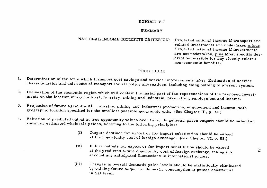
EXHIBIT V.7
SUMMARY
NATIONAL INCOME BENEFITS CRITERION: Projected national income if transport and related investments are undertaken minus Projected national income if investments are not undertaken, plus Most specific description possible for any closely related non-economic benefits.
PROCEDURE
1. Determination of the form which transport cost savings and service improvements take: Estimation of service characteristics and unit costs of transport for all policy alternatives, including doing nothing to present system.
2. Delineation of the economic region which will contain the major part of the repercussions of the proposed investments on the location of agricultural, forestry, mining and industrial production, employment and income.
3. Projection of future agricultural, : forestry, mining and industrial production, employment and income, with geographic location specified for the smallest possible geographic unit. (See Chapter III, p. 34.)
4. Valuation of predicted output at true opportunity values over time: In general, gross outputs should be valued atknown or estimated wholesale prices, adhering to the following principles:
(i) Outputs destined for export or for import substitution should be valued at the opportunity cost of foreign exchange. (See Chapter VI, p. 88.)
(ii) Future outputs for export or for import substitution should be valued at the predicted future opportunity cost of foreign exchange, taking into account any anticipated fluctuations in international prices.
(iii) Changes in overall domestic price levels should be statistically eliminated by valuing future output for domestic consumption at prices constant at initial level.

EXHIBIT V. 7 continued
5. Netting-out intermediate purchases and shifts of productive resources from other regions. For each economic sector determine net income or value added in wages, interest, and profits by either or both methods:
(i) Deductible costs method:
Net sector income = gross output minus purchase of intermediate goods minus wages, profits, and interest of resources shifted into the region from productive employment outside the region.
(ii) Percentage -value -added-method:
Net sector income (Gross output value) x (percentage-valueadded in this sector) minus wages, profits, interests of resources shifted into the region from productive employment outside the region.
6. Increase in national income = sum of increases in net value added for each sector.
0,
83
CHAPTER VI
APPRAISAL OF COSTS AND DETERMINATION OF ALTERNATIVE TECHNICAL SOLUTIONS
The terrain and prospective traffic in any large area usually call
for a transport system made up of two or more modes. A transport
system can be said to have one or more "backbones" or main routes,
from which "ribs" or feeder routes run off in various directions. The
backbone usually will have a higher capacity and a longer average length
of haul than the ribs. Often the backbone will be one mode and the ribs
another in order to minimize capital costs for smaller traffic volumes.
Modes and capacities should vary to suit the traffic and terrain of the
sections they serve. In an integrated transport system, the trunk network
should be of such size, length, and direction to ensure that all parts of the
economy with traffic enough for a small rib can be tied by transport to all
other parts.
The transport systems of developed economies include all modes
(except pipelines in some cases), but only to a limited degree have the
roles of various modes resulted from central planning. Typically, some
parts of a system were built by private enterprise and others by public
funds without coordination among the various agencies. For developing

84
nations today, the efficient approach to integrating a system of various
modes and capacities is investment planning to develop a coordinated
transport system.
The goal of long-run transportation planning is a solution which
minimizes the total social costs of accommodating the expected future
demand for transportation when the repercussions, or feedback, on
demand from changes in transport are fully accounted for. Over a long
time horizon it is possible to plan changes in the basic plant and capacity
of the transport industry; the optimal scale of plant and the latest tech
nology appropriate for the expected demand and availability of scarce
resources can be taken into consideration and implemented.
Transport planning must take advantage of the best information
obtainable on technology, on the relation between costs per ton-mile and
present or expected traffic volume, and on types of traffic and routes.
The basis for a technically sound solution exists when, in addition to in
formation on demand relationships there are data on the cost characteris
tics of the five basic transport modes (road, rail, water, air and pipeline),
as well as any less conventional modes, and when the service differentials
between modes are either unimportant or can somehow be measured in
cost terms.
Unfortunately, little is known about the general cost behavior of
different transport modes under varying topographical, climatic, and
85
geologic conditions. Virtually no systematic effort has been made to
integrate what information is available, categorizing the various techno
logical possibilities to specify in even a general way the conditions under
which each is most feasible. _/ What we now know indicates that the
_/ There is research underway in this general area by the Battelle
Memorial Institute under contract with the Agency for International
Development. A lucid discussion and survey of existing information on
the alternative cost characteristics of the five basic modes is given in
Richard B. Heflebower, "'Economic Characteristics of Transport Modes,"
in Gary Fromm (ed.), Transport Investment and Economic Development
(The Brookings Institution, 1965).
circumstances peculiar to any case are of overwhelming importance and
must be carefully determined: each case must be decided on its own
merits.
Thus, an investigation of the social costs of each separate mode of
the present transport system is one of the most important and difficult
facets of transportation planning. The function of the study is twofold.
First, it reveals both the total level of transport costs and the
relative costs of each of the alternative media. So it can help to determine
if the overall expenditure on transportation is unecessarily high in light
of available technology and resources, that is, if new investment in
86
transport (for physical facilities or for better administration, training
of operating personnel, etc.) appears warranted. Such a cost study can
also indicate whether a high level of total costs could be reduced by
more efficient allocation of traffic between the existing modes by means
short of (or complementary to) investment; for example, through rational
rate-making and taxation policies. Second, an analysis of present costs
serves as the basis for projecting operating costs of the future transport
system. Of course, the extrapolation of present-day costs to predict
future costs must be done carefully, anticipating- -as much as possible-
all changes over time in the underlying determinants of cost. /
_/ General equiproportionate inflation of all prices over time presents
no problem in economic costing- -future costs should be valued in constant
money terms, that is, at present opportunity prices. Financial costing
must be based on current prices, and therefore entails the need to make
some projection of any expected inflation. Any expected changes in
relative prices of transport inputs are relevant, and must be anticipated
to the extent possible, and incorporated into the analysis. Costs for
entirely new modes not presently in operation must necessarily be pro
jected from engineering analysis. For a distinction between financial
and economic appraisal, see p. 87 and especially pages 95-96 below.

87
In the sections that follow a framework for analyzing the costs
of alternative solutions to "transport problems" is presented. The trans
port problem may vary greatly. In one case it may be the need for road
connection and with no alternative media (although there are still the
important alternatives of location, design standards, staging, etc.). Other
cases may involve broad-scale transportation plans for regions, nations,
or even groups of nations. But the underlying cost appraisal is the same:
determining the effective engineering alternatives and estimating the costs
of each alternative to determine the least-cost solution. /
_/ Of course, the services of even very similar alternatives will differ
in greater or lesser degree. This means that a solution cannot be
reached on the basis of costs alone and the analysis must also take into
account the different benefits of each alternative. For this final compo
site analysis, see Chapter VII.
A. Principles of Economic Costing
It is investment planning, the purpose of which is the efficient
allocation of resources to maximize the social and economic objectives
of the country, which concerns us here. Financial planning, which deals
with problems of collecting capital, interest, and operating costs of the
project and securing necessary loans or grants, is not discussed in any

88
detail here. / Six principles, derived both from economic analysis and
/ See pp. 110-113 below.
engineering field experience, apply to transport investment planning:
1. Divergence of input prices from opportunity costs. There are four major instances in which the market prices of production inputs may diverge from their opportunity costs: inputs of skilled and unskilled labor, inputs of capital, inputs which utilize foreign exchange, and inputs upon which sales and other indirect taxes are imposed. For economic planning and thq efficient allocation of the country's scarce resources, these resources should be valued at their opportunity costs; for financial planning and administration they should be valued at their market prices. Ordinarily both calculations should be made.
The opportunity cost of any factor of production in a given use is
the value of the output of the factor in its next-best use which is foregone
when that resource is employed in one use rather than the other. The
opportunity cost of $1 million in capital funds used to build a road is
the value of output which that amount could earn in its next best use, say
a cement plant which is not built because of the lack of funds. Ordinarily
it is assumed that the market price of any factor reflects, or is more or
less equal to, its opportunity costs; this is a basic and necessary tenet
of the free enterprise or competitive economy. Where this relationship
breaks down, evaluation o:" capital projects on the basis of market prices
will not ordinarily lead to selection of that group of projects which contributes

89
the maximum amount to national income. In underdeveloped countries
market prices of some factors may diverge from their true opportunity
costs. Wages of skilled labor, market prices of capital, and foreign
exchange cost components are often undervalued, and the wages of unskilled
labor overvalued. When this situation exists, approximations of opportunity
costs of factors should be provided by the international lending agency
concerned, not by the transport consultants; but if the figures are not
already available from these sources, it will be necessary for the analyst
to estimate them directly. _/ Sales taxes, license fees, and import duties
_/ For further discussion of the concept of opportunity costs (or "account
ing prices"), their relevance to project evaluation, and practical field
techniques of estimation, see Jan Tinbergen, The Design of Development,
Economic Development Institute of the International Bank for Reconstruction
and Development (Johns Hopkins Press, 1958), pp. 35-41, 76-90;
and, especially, Gustav F. Papanek and L%4oeen A. Qureshi, "Use of Account
iig in Prices in Planning," Organization. Planning and Programming for
Economic Development, Vol. VIII of United States papers prepared for the
United Nations Conference on the Application of Science and Technology
for the Benefit of the Less Developed Areas, 1963; and Hans Adler,
"Economic Evaluation of Transport Projects," in Gary Fiomm (ed.),
op. c it.
90
on cost components of the project, which do not reflect opportunity costs,
should be excluded from the estimate of costs for economic appraisal.
2. Sunk Costs. Investments which have already been made and which have little or no value (net of salvage costs) in alternative uses, involve no opportunity cost to the economy; they are either employed in the fixed use or lie idle. Hence they are irrelevant to the new investment decision and are to be ignored. For example, capital costs of an existing railway are to be ignored in considering the profitability of current operation of the present facilities.
Investment planning, even in developing countries, is often con
cerned with additional capacity and extension of existing facihL.,, %. Where
usable facilities exist--even cleared rights-of-ways for a very low quality
rail line or road--only capital charges (depreciation and interest) and
maintenance expenses for the added investment in the new facilities are
relevant. Nevertheless, replacement of the establisheCd mode may be better,
either because of technological advance in this mode or because actual
volume has proved to be so small that relevant out-of-pocket costs of the
established mode would exceed the entire extra costs of the substitute
mode. For example, one study of Argentine railroads concludes that to
rehabilitate and maintain the basic facilities and operating equipment of
a number of existing light-traffic rail lines would involve new-expenditure
costs per ton-kilometer in excess of the total cost of abandoning the rail
road and utilizing parallel highways and operating trucks over them.
91
3. System-wide costs. An estimate of costs for a proposed solution should include all costs to the economy necessary to implement the proposal. A proposed solution may entail necessary expenditures on feeder roads and vehicle fleets and virtually always implies
future maintenance expenditures of some form. The danger of necessary complementary investments being overlooked is greater in the case of the single project appraisal than for overall transportation surveys and planning.
4. Alternative solutions. Investment decisions refer to choices between alternatives; if there were no alternatives, there would be no purpose of investment analysis. There always exists the important alternative between doing something and doing nothing. Therefore, the investment analyst will bear the burden of proof that the recommended project is actually the preferred one considering all circumstances.
Many alternative solutions to any given transportation problem
may exist. There are fundamental alternatives among modes or combina
tions of modes--whether road, rail, water, pipeline, or air. In many
cases, choice among modes will not be an issue because terrain, traffic
characteristics, nearness to existing facilities (in rail and water systems),
and other factors make the solution self-evident; in other cases, a choice
among alternative modes will constitute the primary issue. In any case,
the investment study must explicitly demonstrate that the proposed
solution is the preferred one. A major weakness of many earlier transport
studies was their failure to analyze the prospects of intermodal, substitu
tabilities and complementarities.

92
Important nontransport alternatives may exist. Various ways
of processing the goods which constitute the potential traffic may be
alternatives to transport. This is true for many agricultural and other
raw materials. Another alternative is the substitution of long-distance
high-voltage transmission of power from hydroelectric sources for hauling
coal from collieries to thermal power plants. In some situations a choice
of location of industry may be preferred to improved transport. Plant
locations involve a trade-off between the economies of scale in plant con
centration and the increased cost of transport to the wider markets
necessary to support a large plant. When economies of large scale are
relatively important, the demand for transportation will be greater, and
vice versa. India is one country in which increasing attention is being
devoted to the trade-offs between plant scale and transport costs.
Another major group of alternatives for appraisal centers on the
choice of design standards and spacing over time. Even if the future
traffic is completely certain, there are important trade-offs between
present capital expenditures and future capital and maintenance expendi
tures.
If a rapid rate of traffic growth is expected, it may be efficient
to incur high present capital costs by building to high standards in order
to avoid the much higher costs of expanding lower standard facilities in
the near future when traffic demands exceed their capacity. For example,
93
it may be much cheaper to build a four-lane bridge now rather than one
two-lane bridge now and another two-lane bridge within ten years.
However, for a rural road with small present traffic volume it may be
best to build the road base to high standards, but provide only a low
grade bituminous surfacing until traffic growth warrants a heavier
surface. Although higher user costs may be incurred now, these may be
more than offset by savings on capital costs.
The opportunities for such "staged construction," increasing
capacity by small increments over time to accommodate only actual
traffic increases, should never be overlooked. By building to high standards
now and incurring high present capital costs, much future expenditure on
maintenance can be avoided; or by building to low standards, much
present capital cost can be (not avoided but) postponed in the form of
high future maintenance costs. In general, the best solution depends on
three factors: (1) the relationship between design standards, volume of
traffic, and maintenance costs; (2) the relationship between the costs of
constructing high capacity now and expanding capacity later; and (3) the
rate of interest at which future costs are discounted to compare with
present costs.
Uncertainties, which are bound to be great, require policies which
tend to minimize the impact of surprises. Ordinarily, this will have the
effect of discouraging high present standards and postponing outlay wherever
94
possible. The American engineer .;ho is conditioned by highway trans
port in the United States, where it makes sense to build to high standards
well ahead of a rapidly growing demand, must understand at least two
circumstances which are different in the less developed countries.
The expected rate of traffic growth is often much lower and the
uncertainties are always much greater. While there are examples where
the building of modern high-capacity transport facilities resulted in
dynamic new economic growth with a proportional increase in traffic,
there are also many examples of new transport developments lying waste
fully idle.
The opportunity cost of capital (rate of interest) may be much
higher than in the United States, which means that future costs are
valued less highly relative to present costs. This implies, for example,
that standard charts which portray the optimal trade-offs between present
design and user costs and future maintenance costs based on experience
in the United States are wholly inapplicable to the underdeveloped countries. /
_/ No such tables which are applicable under a completely general range of
conditions are known to exist. See footnote on page 85.
5. Time profile of costs. Some costs, such as capital costs, are incurred immediately, while others, such as
95
maintenance costs, are incurred at a later date.
Since we know that a dollar expended today is worth
more than a dollar expended ten years from today
it is vitally important to identify the specific form
of the costs flow over time. The point in time at
which each expenditure is expected to occur must be
noted, and the entire stream of anticipated expendi
tures should be in the form of the "time" profile
diagram illustrated in Exhibit VI.l. Note that no
amortization or depreciation payments should be
included in the economic analysis, only the actual
capital cost, maintenance, operating cost, and inven
tory costs as they are incurred. Of course, it is essential that the anticipated amortization and depreciation schedules be presented explicitly in the financial analysis.
6. Confidence limits for cost estimates. Past experience
indicates that estimates of construction costs for capital projects are subject to wide errors, usually understating
the actual costs which are ultimately incurred. The
costs estimator should determine both a single most probable estimate and confidence limits, an outside high
and an inside low estimate within which actual costs
may reasonably be expected to fall. The analyst should consult with the international lending agencies so as to
benefit from previous cost experience within that country.
B. Transport Cost Components
It is necessary to determine the time profile of economic costs for
each possible investment considered, always including the alternatives of
undertaking no invrestment or even abandoning present transport services.
It is social cost as distinct from financial outlay or outlay of the carrier
which is relevant to the economic analysis. Social cost of transportation
is the value of resources which are actually consumed in the transport of
96
the traffic from the door of the shipper to the door of the receiver.
Social cost thus includes not only carrier costs but also those costs
which are incurred directly by the shipper; for example, the costs of
packaging for transport and interest charges on inventory.
The financial analysis will define costs from the point of view of
the carrier company or public transport authority, including all money
outlays but nothing more.
Here we refer exclusively to the economic or social costs. The
necessary degree of refinement in costs information will vary from case
to case. It need never go beyond the point at which it is possible to
make a conclusive determination of the preferred solution. Of course,
the main consideration will usually be the scarcity of data available to
make a scientific determination of costs within any acceptable limits of
confidence.
1. Capital Costs
Capital costs are the costs of the basic facilities and equipment.
Basic facilities such as terminals, highways, railroad tracks, and
related structures ordinarily have a much longer life span than the
equipment, such as trucks, rail rolling stock, or cargo handling equipment.
(See Exhibit VI.l[aj.)
Estimation: Cost all nonrenewable existing facilities at net
salvage value, if any. This will ordinarily exclude a large part of the
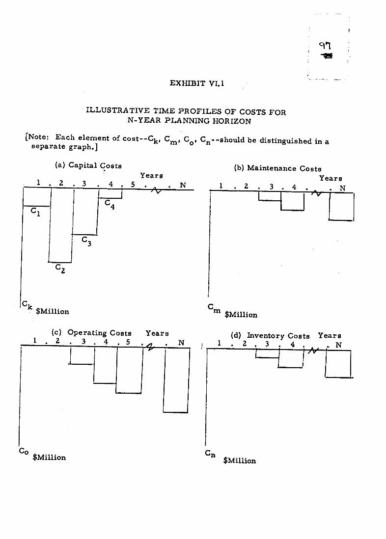
EXHIBIT VI.1
ILLUSTRATIVE TIME PROFILES OF COSTS FOR N-YEAR PLANNING HORIZON
[Note: Each element of cost--Ck, Cm, C I C- -should be distinguished in a separate graph.]
(a) Capital Costs (b) Maintenance Costs Years Years1 2 .3 4. N 1. 2 .3.4 N
C 1 C Cl
C 3
C2
$kMillion mr $Million
(c) Operating Costs Years (d) Inventory Costs Years I .2 3 4 5 * N 1 2.n N
Co $Million Cn$Million
98
capital costs of the present basic facilities, such as highways and
structures, rail beds and structures, and port structures. On the other
hand, terminal buildings, warehouses, and equipment will usually have
some net salvage value.
The time profile of capital costs of new construction and equip
ment (including costs of future capital replacements for the present
system) will be determined by standard engineering practices. (See
Exhibit VI.l[a] )
2. Maintenance Costs
Maintenance costs are the outlays necessary to keep the basic
facilities and equipment in operation. Maintenance is in part a function
of the amount of usage and in part a function of aging.
Estimation: The time profile of annual maintenance costs for
proposed facilities and equipment will be determined by engineering tech
niques; maintenance costs of existing facilities and equipment may be
determined either by engineering estimates, or by any of the methods
of estimating operating costs discussed below. (See Exhibit VI.l[b].)
3. Operating Costs
Operating costs are those costs necessary to carry the traffic
over the basic facilities. They are incurred mainly by the carrier
companies and they vary in response to the volume of traffic over the
basic facility.

99
The operating costs of each different mode of transport will
respond in a different way to varying traffic characteristics (such as
average length of-haul, size of shipment, passenger and commodity mix,
speed and frequency of service) and physical circumstances (such as
terrain and climate). Broad averages based on system-wide totals of
operating costs and gross ton-miles of traffic reflect the net effect of
these many varying and sometimes opposing tendencies. They are un
satisfactory to use for estimating costs in any specific investment
situation, except where it can be shown that the various cost determining
factors are quite similar in the specific case.
Estimation: It is important, first of all, to identify the funda
mental cost-determining factors in the specific planning situation so that
the analysis can be directed toward the relevant circumstances.
The estimates of annual operating cost should be derived in the
following way: for proposednew facilities determine average operating
costs on comparable facility under similar conditions elsewhere in the
same country by standard engineering practices or other costing
techniques, discussed below; J estimate present costs over existing
/ See section C, pp. 102ff.
facilities directly if possible, otherwise estimate on the basis of compa
rable facility including allowance for increasing unit costs due to
100
congestion where necessary. Multiply expected traffic volume for each
year by the estimated average costs to determine the time profile of
annual operating costs as shown in Exhibit VI.l(c).
4. Inventory and Other Costs.
Inventory costs reflect the time consumed in and the uncertainty
of, transport. Ordinarily the shipper must tie up capital funds in the
volume of goods being transported, and the interest charges on these
funds represent an inventory cost which is greater the longer the time
required in transport. Similarly, if transport service to any specific
location is infrequent, then business firms there must invest in inven
tories of the products which they buy and sell, and the less frequent the
service the greater the interest costs. Again, regardless of the average
length of transport time and the average frequency of scheduled service,
if the service is not reliable, then larger inventories and inventory costs
will result. Closely related costs are due to spoilage losses which may
occur when perishable commodities are detained too long in transit; we
include these under inventory costs here. Transport modes vary with
respect to speed, frequency, and dependability. These service charac
teristics can assume pivotal importance in determining the best means
of transport. (See Exhibit VI.l [d].)
Estimation: Inventory costs may be approximated by the following

101
formula:
Annual Inventory Costs = (V) x (D) x (i) x (t/365)
where:
V = Average value per ton of existing or projected traffic.
D = Number of tons originating of existing or projected traffic, i.e., annual number of tons shipped.
i . (Opportunity) annual rate of interest.
t a Average number of days in transit, from door of shipper to door of receiver.
Because this measures only interest charges on goods in transit,
it is not an all-inclusive measure of inventory costs, but an underestima
tion of the actual. / However, it may often be such a large component
/ For a discussion of the concepts of inventory costs in transportation
and an important application thereof, see John R. Meyer, Merton J. Peck,
John Stenason, and Charles Zwick, The Economics of Competition in the
Transportation Industries (Harvard University Press, 1959), pp. 189-193,
348-353.
of inventory costs that the study costs of deriving more refined estimates
are unwarranted.
Losses due to damages in handling freight are costs of transport
and may be important in some phnning situations. Damage claims paid

102
by the carrier may provide a major source of data, but they may also
understate actual losses considerably. A survey of shippers or possibly
insurance companies, may provide enough supplementary information
for a more statisfactory estimate. The estimate should be defined for
each year of the planning horizon.
Exhibit VI.l(d) illustrates a time profile of inventory and associated
costs.
C. Estimation of Operating Costs: Sources of Information and Techniques
of Analysis
Estimating transport operating costs is important and difficult.
Four approaches to cost estimation are outlined below. They are not
alternative techniques but complementary tools to be used jointly
wherever possible in attempting to construct a factual profile of this
elusive subject. Each estimate can be used as a cross-check against
every other estimate and in this way a much firmer estimate can be had than
by using any single approach. The four basic approaches discussed
below are: (1) rate surveys, (2)conventional cost accounting, (3)
engineering costing and controlled cost accounting, and (4) statistical
costing.
1. Highway rates surveys. The basic tenet of the rates survey
is that, in certain circumstances, the rate charged by highway carriers
(and sometimes inland water carriers) for a particular movement reflect
quite closely the costs incurred in that movement; any profit is small,
103
reflecting only risk-taking and the "normal wages" of management. This
tenet is generally true, and the method is appropriate for highway
carriers in a highly competitive situation where there are many small
carriers, such as one-truck operators, and no collusive rates agree
ments are in effect.
Rates charged will reflect some allowance for depreciation of
vehicles, other equipment, and facilities incurred by the carrier firm.
(No allowance may be included in unusual and extremely competitive
situations.) These charges must be subtracted from the rates since they
are already included under capital costs. They may be estimated by any
of the other three costing approaches.
Rates actually charged, as distinct from quoted or published
tariffs, must be used. These can be ascertained by an interview survey
including carriers, shippers, and traffic brokers (if any).
2. Conventional cost accounting. This approach may be used in
larger transport companies to determine average unit costs of particular
operations under varying conditions. These accounts may be available
privately, or from carriers' associations or regulatory authorities; and
total costs of specific movements can be built up from them. Again,
any allowance for depreciation of vehicles and equipment included else
where should be excluded here.
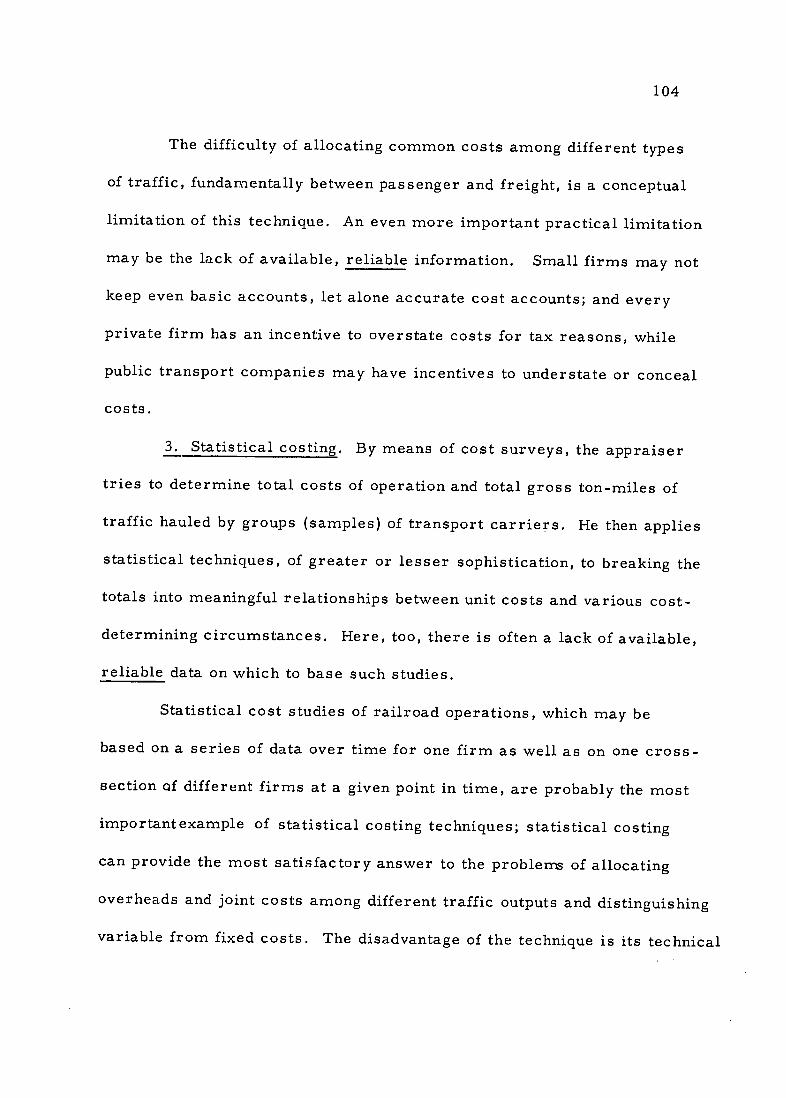
104
The difficulty of allocating common costs among different types
of traffic, fundamentally between passenger and freight, is a conceptual
limitation of this technique. An even more important practical limitation
may be the lack of available, reliable information. Small firms may not
keep even basic accounts, let alone accurate cost accounts; and every
private firm has an incentive to overstate costs for tax reasons, while
public transport companies may have incentives to understate or conceal
costs.
3. Statistical costing. By means of cost surveys, the appraiser
tries to determine total costs of operation and total gross ton-miles of
traffic hauled by groups (samples) of transport carriers. He then applies
statistical techniques, of greater or lesser sophistication, to breaking the
totals into meaningful relationships between unit costs and various cost
determining circumstances. Here, too, there is often a lack of available,
reliable data on which to base such studies.
Statistical cost studies of railroad operations, which may be
based on a series of data over time for one firm as well as on one cross
section of different firms at a given point in time, are probably the most
importantexample of statistical costing techniques; statistical costing
can provide the most satisfactory answer to the problems of allocating
overheads and joint costs among different traffic outputs and distinguishing
variable from fixed costs. The disadvantage of the technique is its technical

105
sophistication and high costs. /
_/ For a discussion of the techniques, their suitability, and an important
application to U.S. Railroads, see Meyer, et. al., op. cit., pp. 27-63,
277-327. See also A. A. Walters, "Production and Cost Functions: An
Econometric Survey," Econometrica, V. 31 (January-April, 1963), pp.
39-52.
4. Engineering costing and "controlled" cost accounting. By
these techniques an attempt is made to determine technical input coeffi
cients of each operation of the transport movement, such as the input of
fuel required to move one gross ton-mile of freight over a road of a
specified gradient and surface type, all other factors being held constant.
Total costs of any specified movement are then built up from these
coefficients. This approach involves some form of 'engineering experi
ment or cost accounting in an actual transport operation with controlled
conditions. The methods can be used to allocate joint costs among
different traffic types and yield more reliable information than conven
tional techniques. However, since they are rarely, if ever, available
from the carriers' own accounting operations, these techniques involve
significant study costs.

106
D. Summary
A summary of the basic principles, required information, sources
of data, and techniques of analysis for costs appraisal is presented in
Exhibit VI.2.
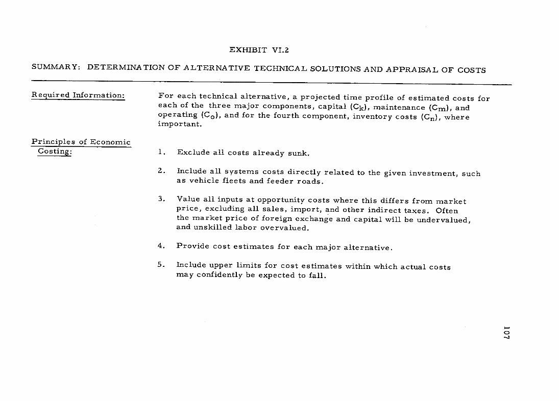
EXHIBIT VI.2
SUMMARY: DETERMINATION OF ALTERNATIVE TECHNICAL SOLUTIONS AND APPRAISAL OF COSTS
Required Information: For each technical alternative, a projected time profile of estimated costs for each of the three major components, capital (Ck), maintenance (Cm), and operating (Co), and for the fourth component, inventory costs (Cn), where important.
Principles of Economic Costing: 1. Exclude all costs already sunk.
2. Include all systems costs directly related to the given investment, such as vehicle fleets and feeder roads.
3. Value all inputs at opportunity costs where this differs from market price, excluding all sales, import, and other indirect taxes. Often the market price of foreign exchange and capital will be undervalued, and unskilled labor overvalued.
4. Provide cost estimates for each major alternative.
5. Include upper limits for cost estimates within which actual costs may confidently be expected to fall.
-

EXHIBIT. VI.2 - continued
Mode Required Information
Highway Rates survey for conditions similar to cost determinants of problem at hand to estimate both:
(i) present costs (ii) costs on pro-
posed facility,
Highway Costs estimate as specific as possible with respect to the cost determinants of problem at hand for both:
(i) present costs. (ii) costs of pro
posed facility
Source of Data
Survey of truck carriers, shippers, and traffic brokers,
Caution: actual rates may differ from published or "quoted"rates
Trucking firms. Trucking asso-ciation. Regulatory boards.
Highway research organizations or direct experiment,
Techniques of Analysis
Direct determination of rates over given route or routes with similar cost circumstances to case being studied.
Conventional cost accounting.
Simple statistical analysis of sample conventional cost accounting.
Engineering experiment and controlled cost accounting.
Advantages
Low cost. Available in detail for different
circumstances. Can be quite reliable
Low cost. Most readily available, simple to understand.
Can determine representa-tive costs
under wide range of cost circumstances.
Accurate information, Experiment
can be tailored for specific problem at hand.
Disadvantages
Inappropriate for noncompetitive situation, where carriers are few or rates
agreements exist.
Inaccuracy of reported data.
Moderate cost. Inaccuracy of reported data. Possible errors
of statistical analysis
Moderate to high cost. o
CO

EXHIBIT. VI.Z -'continued
Mode Required Information Source of Data
Railway (same as for highways) Railway Co.: Published or internal data. Regulatory authority reports.
(Same as above)
Techniques of Analysis Advantages Disadvantages
Conventional cost Most readily (i)Averages for accounting. available, different types of
Relatively passenger and inexpensive. freight services,
different lengths of haul, different parts of the system conceal important variations. (ii) Difficult to allocate overheads among joint output.
(iii) Difficult to distinguish variable from fixed capital costs, and distinguish
incremental costs from average costs.
Controlled cost experi- Can break Difficult to mentation distinguishing down allocate between operational cost averages passenger and components. to distin- freight services.
guish among Also same as different freight
(ii) and (iii) of conventional
o
services and cost accounting.
different lengths of haul.
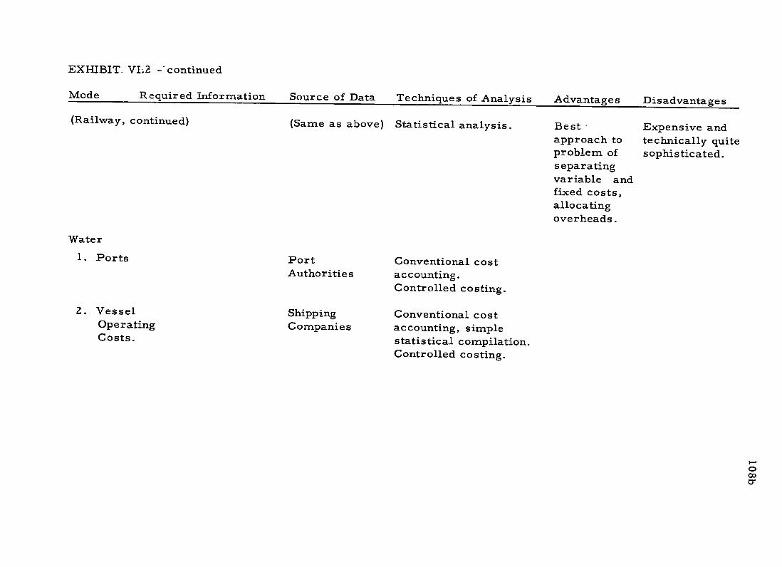
EXHIBIT. VL2 -'continued
Mode Required Information Source of Data
(Railway, continued) (Same as above)
Water
1. Ports Port
Authorities
Z. Vessel Shipping Operating Companies Costs.
Techniques of Analysis
Statistical analysis.
Advantages
Best-
approach to problem of
separating
variable and fixed costs, allocating overheads.
Disadvantages
Expensive and
technically quitesophisticated.
Conventional cost
accounting.
Controlled costing.
Conventional cost accounting, simple statistical compilation.
Controlled costing.
300 Cr

109
CHAPTER VII
DECISION CRITERIA FOR CHOOSING AMONG ALTERNATIVE INVESTMENT POSSIBILITIES
The purpose of the pre-investment appraisal is three-fold: (1) to
establish the engineering feasibility of proposed projects and to determine
all technical and administrative requirements necessary to provide a
viable, effective transport service; to provide(2) cost estimates upon
which necessary financial arrangements can be based; and (3) to choose
from a broad range of alternatives that particular solution which will
result in the maximum possible gain to the country concerned. It is
primarily this choice of the "best" project from the point of view of
national welfare to which this manual is directed.
Previous chapters have discussed individual components of the
investment analysis: the resource and industrial base, the demand and
supply of transport services, and the benefits and the costs of individual
transport projects. In the present chapter these various factors are
brought together and integrated into a formal framework for comparison
and choice between alternatives.

110
A. Financial Versus Economic Criteria /
/ Refer to Robert Sadove and Gary Fromm, "Financing Transport
Investment,"' in Gary Fromm (ed.), Transport Investment and Economic
Development (Brookings Institution, 1965), pp. 224-241.
A maximum contribution to the national welfare is indicated pri
marily by the expected increase in national income, but it also includes a
contribution to other economic and social goals, such as more equal income
distribution, improved medical care, political unity, and similar objectives.
The national welfare goal specifies basically economic criteria for decision
making. Projects chosen on the basis of these criteria may differ from
those which would be chosen on some other basis.
Projects are also appraised on the basis of financial criteria--by
their ability to generate revenues equal to the expenses of the undertaking
plus a "fair return." Conceptually, four policy situations can be distin
guished when both criteria are employed: (1) both criteria agree to reject
the proposal; (2) the economic criterion rejects the proposal while the
financial criterion accepts it; (3) the economic criterion accepts the
proposal while the financial criterion rejects it; and (4) both criteria agree
to accept the proposal.
There is no conflict in cases (1) and (4), since economic and finan
cial criteria agree. In case (2) the two criteria conflict but no policy

dilemma is presented since it is ordinarily easy to reject a proposal, to do
nothing. The main cause of such a situation is the existence of important
divergences between the market prices and the true opportunity costs of
various inputs. This is particularly true of inputs with market or financial
prices which understate their true economic cost, such as scarce foreign
exchange, capital, and skilled labor. The project may also have undesirable
effects ("external diseconomies") which the economic analysis will include
and the financial analysis ignore. An example would be increased costs in
other industries which use the same inputs as transport. If the objective
is the economic development of the country, it is clear that any project
which is unjustified by economic criteria, even though it may be financially
attractive, must be rejected.
It is only in case (3), where a project meets the economic criteria
but cannot pay its own way, that an important policy problem arises: a
subsidy must be raised to support the project if it is undertaken. Before
such a course is rejected, there are certain possibilities which should be
examined. First, a project which cannot raise its own expenses and interest
may have important favorable effects ("external economies") on the profit
ability of other enterprises. These effects may not be reflected in transport
revenues but may serve to increase the national income. Second, a project
may be financially unattractive but still represent the maximum contribution
to the national income because it is forced to pay out the market prices of

112
some factors (particularly unskilled labor) which do not reflect their true
scarcity value to the economy. Thus in the extreme case where labor is
otherwise unemployed, the economic opportunity cost of the labor is nil,
while the financial costs in wages paid out can still be considerable.
However, when a subsidy is necessary to an enterprise, the funds
must be raised either by additional taxation, government borrowing, or
by reducing expenditures on other public undertakings which may be
economically just as good or better than the given proposal. Therefore:,
it will be necessary to undertake careful, broader studies to determine the
sources of subsidy funds and the return on any projects, public or private,
which would be reduced or abandoned by reallocation of public funds or
forestalled by taxation. This will, in effect, determine the true opportunity
cost of the investment funds (see Chapter VI, pp. 87-89). The economic
profitability of each proposal can then be recomputed, using the new oppor
tunity cost of the funds, depending on the source from which they are
derived. The highest ranking project can then be chosen for implementa
tion.
Of course, this analysis will not ordinarily be an easy undertaking.
It is necessary only when financial and economic criteria conflict and the
capital sums involved are large. In view of the high costs of such studies,
the sensitivity of the decision to different costs of public subsidy funds
should first be examined by assuming a plausible range of different values
113
of these funds and then observing the effect on the choice of the project. (See
pages 148- 150.) Only if the decision is strongly affected by variations in the
value assumed by the subsidy funds will it be necessary!to proceed with
intensive analyses to determine the true opportunity costs of those funds.
Then it will require the most expert economic consideration.
Despite all these considerations, a financial analysis of every capital
project proposal given serious consideration is important. An analysis of
the anticipated income and expenditures profile of the project is the only
basis upon which necessary financial arrangements car. be secured. The
point here is that financial analysis is not relevant to the choice of one
project rather than another. This is a matter to be determined by economic
analysis.
B. Formulating the Problem Correctly
The "optimal" solution chosen can only be as good as the alterna
tives that are considered; the best criteria cannot lead to good projects if
only poor ones are considered. Thus, much of the difficult task lies in the
specification of effective technical and administrative alternatives in the
problem under consideration. There can be no substitute for the specialized
knowledge of the combined team of engineering and economic experts.
The range of alternatives which the investment appraisal entertains
will profoundly affect the wisdom of the final selection. For example, if
114
the problem is transporting coal, a large part of which is for thermal
production of electricity, the possibility of hydroelectric production and
transmission by high-tension power lines to markets should be considered.
If it is arbitrarily ruled out, a less-than-optimal solution may be proposed.
At least six different types of alternative actions can be distinguished in
transportation planning:
1. Allocation of investment funds between transport and
other industries.
2. Allocation of investment funds between transport and
transport substitutes.
3. Choice among different transport modes.
4. Choice among different scales or design standards for
each project and their spacing over time.
5. Improvements in regulations and administrative and
operational efficiency which would increase the effective
capacity of the existing system.
6. Rationalization of rate and tariff structures toward
more efficient utilization of present transport services.
In nny planning situation, the analyst must carefully weigh the
aavantages and disadvantages of expanding the range of alternatives
which he considers. Ordinarily, the transport analyst does not confront
alternative (1) directly. He may approach it indirectly by comparing the

115
rate of return on transport investments with the "going market rate" on
similar investments in public utilities or large-scale industry or agricul
ture. He may deal with at least that part of alternative (2) which involves
a comparison of additional investment in transport capacity with, fo:.'
example, the most obvious alternatives in storage facilities, processing
plants, and containerization. However, his responsibility may not encom
pass the relocation of industrial development. The analyst must compare
the importance of expanding the study with the costs of doing so.
The sphere of interest of the transport study will always include
alternatives (3), (4), (5), and (6), which are now discussed.
If an alternative transport mode (3) is feasible, perhaps because a
navigable river or an existing trunk rail line lies on or near the route,
choice between the modes is a question which must be considered. Perhaps
a single mode or a combination of modes will be warranted. Since the
services which different transport modes produce may differ substantially,
it will be necessary to ccompare careflly the different costs and benefits
of each. For example, the speed of service will be different between road
and rail, and between rail and water. The interest charges on the goods
while in transit, which will vary also with the value of the cargo, must be
taken into account.
One of the most important alternatives which must be considered is
the choice of the optimal scale or design standard of the particular facility

116
is chosen, and its spacing in time (4). Ordinarily the very minimum
facility capable of handling the present traffic should be adopted as a
base for comparison, and any expansion in scale or other enhancement
in design standard must be appraised on its own worth; each increment
in expenditure must be considered as an alternative project and must be
separately appraised.
Example 1:
(Detailed numerical calculations for this case are given on pages 144- 147.) There is a proposal to bdild a new quay with berthing space for two ships to relieve congestion and delay in a crowded port. Calculation shows that the whole project, which costs $10 million, yields a positive rate of interest in the country concerned, and the project is approved.
However, if separate calculations were made for each additional berthing space,'it would be revealed that the first space, costing $6 million yields a return far in excess of the opportunity rate of interest. However, the second space which costs $4 million but will be used much less, yields a negative present value when evaluated at the opportunity rate. Clearly, the first space, but not the second, should be built.
Example 2:
A proposal is made to construct an 18-foot wide paved road into a major new colonization area. Combining the costs of the proposed highway with the other inputs in housing, irrigation, and fertilizer (since all inputs are necessary to produce the given output) and comparing costs with the net increase in national income reveals a positive present worth at the given opportunity rate of interest. The project is approved.

117
However, traffic in the first five years of the project will be very light, and the opportunity cost of capital investment in the highway will be high. A comparison of the plan that was adopted with an alternative identical in all respects except for construction of a two-lane gravel road at first and reconstruction five years later into a paved highway (commensurate with the increased volume of traffic at that time), reveals a much higher net present worth for the latter plan, which should be adopted.
The circumstances within which the transport system is to
function- -particularly the legal regulation, efficiency of administration,
availability of technically skilled people, and availability of adequate main
tenance funds and spare parts (5)--must be considered in the final deter
mination. While investments in competent admiiiistration, technical
training, and proper maintenance usually return high dividends, these
complementary resources are not automatically guaranteed; and new
arrangements in this respect may require long gestation periods before
yielding output. The transport planner must either make sure that the
complementary resources are available or outline the appropriate policies
necessary to secure them for the particular transport solution which he
recommends.
Transport rates (6) for different types of traffic may not reflect
the actual costs of hauling that traffic. There are circumstances in which
distortions between rates and costs are economically sound. However, these
distortions often arise because of government regulation of rates which
favors particular classes of users--such as passengers against freight or
118
vice versa. Discriminatory regulations may be due to implicit value
judgments, tradition, or (most commonly) ignorance of actual costs. In
such cases, more rational rate making, by reallocating various traffics
to the lowest cost media, or by choking off entirely wasteful, uneconomic
movements can result in impressive reductions in a nation's total transport
expenditures and actually increase the capacity of the system. Th' cost is
extremely modest compared to investment in additional physical facilities. J
_/Cf. Edwin T. Haefele, Government Controls on Transport: An African Case
(Brookings Institution, forthcoming).
In any case, the issues involved are quite complex and where evidence exists
that rates are an important issue, employment of an expert is indicated.
C. Uncertainties and Risks in Evaluating Costs and Benefits.
Experience has shown that there is a great deal of uncertainty in
predicting the benefits and costs of a proposed project. The passage of
time has often revealed wide divergences of actual costs and benefits from
those originally predicted in the pre-investment appraisal. More often than
not, the passage of time reveals errors which underestimate costs and over
estimate benefits. This creates a bias favorable toward the project.
More careful application of more expert methods of estimating bene
fits and projecting costs and benefits will eliminate many errors. However,

119
a great degree of uncertainty will always remain in such projections. The
traditional method of handling these uncertainties has been to allow for
"contingencies" by increasing the estimates of costs and/or decreasing
the estimates of benefits by an arbitrary amount based on previous experi
ence, intuition, random guess.or a Such a procedure is conceptually sound
and can be of great practical value when it has some logical basis such as
previous experience under similar conditions carefully interpreted. Uncer
tainties have also been handled by applying a high rate of interest as a
discount of the risk involved in such investments. This is, of course, one
function of the rate of interest in a free-enterprise economy. It is reflected,
for example, in the difference between the rate which is charged a small
borrower and that charged a larger and safer borrower.
The method for coping with uncertainties recommended here involves
a combination of techniques. It includes the use of an appropriate rate of
interest for discounting risks and a "sensitivity analysis"--making various
contingency assumptions with respect to the main variables to determine
those which most importantly affect the analysis. First, the rate of interest
used in the investment analysis should be the market rate of interest on the
most similar type of private investmeint in the economy-. (See pp. 138 141.)
This in effect assumes that the predictive ability of the transport planners is
no better or worse than that of the private investor in the economy; if it is
worse, the rate charged should be higher, and if the risk of the public invest

120
ment is less, the rate of discount should be less. Second, a range of
assumptions--at least an optimistic and a conservative extreme--should
be assumed for each major variable affecting costs and benefits. These
can then be "tried out" on the investment calculations to determine their
effect on the decision of what project to adopt, if any. (See pp. 148-150.)
Obviously, if the choice of the project is not much affected by the variations
in the value assumed by a given variable, it is not important to obtain a
more accurate estimate of that variable. In some rare situations, one
project will be preferred under one realistic set of assumptions, and another
project will be preferredon the basis of another set of realistic assump
tions--and no amount of expert analysis at the present time can narrow the
probable range of behavior of the variable(s) involved. In these circum
stances, experienced judgment, with an awareness of the importance of the
various assumptions, must be exercised.
D. The Investment Decision
1. Computing present values of future benefit and cost streams.
All criteria for public investment choice are based on a comparison
of the discounted present value of the future stream of social benefits, B0 ,
with the discounted present value of the stream of social costs, C0 , of each
project in relation to every other alternative project. Here only a definition
and a brief description of the computational method for discounting future
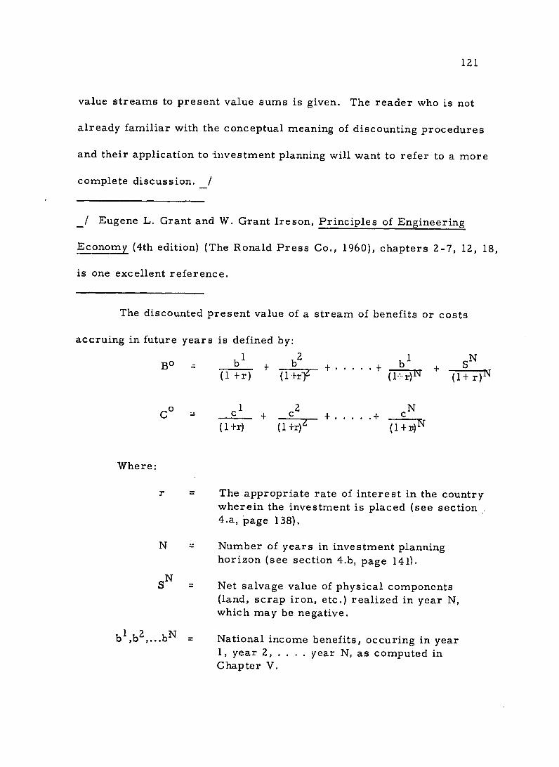
121
value streams to present value sums is given. The reader who is not
already familiar with the conceptual meaning of discounting procedures
and their application to investment planning will want to refer to a more
complete discussion. /
_/ Eugene L. Grant and W. Grant Ireson, Principles of Engineering
Economy (4th edition) (The Ronald Press Co., 1960), chapters 2-7, 12, 18,
is one excellent reference.
The discounted present value of a stream of benefits or costs
accruing in future years is defined by:
BO b 1 b ..... + b1 SN
(1 +r) (l+r) +.-.-r+ (1+ r)'
° b1B .. b Nir~ (1r 2 cNc +......+c +
)N (1+r) (I +r
Where:
r The appropriate rate of interest in the country wherein the investment is placed (see section 4.a, page 138).
N Number of years in investment planning horizon (see section 4.b, page 141).
S N Net salvage value of physical components (land, scrap iron, etc.) realized in year N, which may be negative.
bl,b2,...bN National income benefits, occuring in year 1, year 2, .... year N, as computed in Chapter V.

122
c1 c .... N Total of all capital, maintenance, operating,
and inventory costs occurring in year 1, year 2, . . .year N, as computed in Chapter VI.
The present worth factors 1 1 , . . can, of course, (l+r) (1 +r)
be determined for any rate from any standard interest tables.
This formulation implicitly assumes that the benefits or cost values
which may actually accrue continuously over each day of any given year,
fall due or are collected on the last day of that year. This approximation
rarely introduces any consequential error. It should also be noted that a
present value comparison of this nature between any two investment projects
must be based on an equal time horizon, N. It is not correct to compare
one project with a 15-year horizon of benefits and costs, say, with another
project with a 10 year horizon; the comparison must be expanded to a common
denominator, for example, 30 years._/
_/ For elaboration on these and other matters see the text by Grant and Ireson, op. cit.
2. Problems in the choice of a decision criterion. In investment
planning commonly there are a number of mutually exclusive alternatives
from which only one investment project must be selected, and often also
there are not enough investment funds available to undertake every indepen
dent project which would yield some net gain (with a benefit/cost ratio
greater than one). Therefore, there must be some way of choosing the
project or projects that would result in a greater net gain to the economy

123
of the country concerned than some other project or set of investment
projects.
The basic criterion for choosing the best capital project from
among alternatives is the anticipated benefits and costs of each project
compared with those of every other alternative. In practice, there has
been much confusion over the last several years about the precise form
which this comparison should take, whether it should be the difference
between discounted benefits and costs, B 0 - C0 ; a ratio of discounted bene
fits to costs, BO/CO; the internal rate of return, IRR, of each project; or
some other form. Fortunately, careful studies have now yielded conclu
sive answers to this question. A simple benefit -cost ratio will often lead
to the erroneous implementation of investments which do not result in
the largest net gain or benefit to the economy. Unfortunately, the same
statement is applicable to the recently fashionable internal-rate-of-return
criterion. These matters are briefly discussed here and references to the
relevant literature are provided for those interested in a fuller treatment.
V0a. Net Present Value, = BO- C0
Since the overall objective is to maximize net benefits, as described
in Chapter V, it would seem immediately apparent that one correct pro
cedure would be to choose that project (or group of projects) with the
largest discounted net benefit, VO. Indeed, it is true that a decision rule
based on the difference between the discounted present value of future

124
°benefits and costs, BO- C , invariably points to that project which will
make the maximum contribution to benefits under the same circumstances.
It is also true that this rule is ordinarily the simplest criterion to com
pute and apply in actual investment planning. Therefore, it is this criterion,
V° = B 0net present value or - C° , which is devclcped here and which should
be used in evaluating capital projects in transport. _/ An example will
_/ The net-present-value criterion is discussed more fully below, pp. 135- 144.
For both conceptual and practical justifications of the criterion proposed
here see Roland N. McKean, Efficiency in Government Through Systems
Analysis (John Wiley & Sons, Inc., 1958), pp. 76-92, 116, 124; and
J. Hirshleifer, J. G. DeHaven, and J. W. Milliman, Water Supply: Economics,
Technology and Policy (University of Chicago Press, 1960), Chapters VI
and VII.
The annual-net-benefits and annual-net-cost rules, when correctly
applied, are logically equivalent to the net-present-value rule proposed
here, and thus yield the correct decision, but they involve one additional
computational step. They may be used where the individual is so familiar
with this way of thinking that this convenience offsets the additional com
putational burden.
help to make this clear.
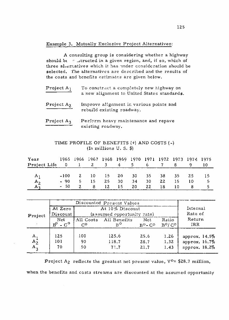
125
Example 3. Mutually Exclusive Project Alternatives:
A consulting group is considering whether a highway should b " .. tructed in a given region, and, if so, which of three alucrnatives which it has -inder ccrisideration should be selected. The alternatives are described and the results of the costs and benefits estimates are given below.
Project A1 To constract a completely new highway on a new alignment to United States standards.
Project A 2 Improve alignment in: various points and rebuild existing roadway.
Project A 3 Perform heavy mairitenance and repave existing roadway.
TIME PROFILE OF BENEFITS (+) AND COSTS (-) (In millions U. S. $)
Year 1965 1966 1967 1968 1969 1970 1971 1972 1973 1974 1975 Project Life 0 1 2 3 4 5 6 7 8 9 10
A 1 -100 2 10 15 20 30 35 38 35 25 15 A 2 - 90 5 15 25 30 34 30 z 15 10 5 A3 - 50 2 8 12 15 20 22 18 10 8 5
Discounted Presenit Values
At Zero At 1076 Discount Internal Project Discount (assumed opportunity : ate) Rate of
Net All Costs All Benefits Net Ratio Return C °B - Co Bo B - CO BO/CO iRR
A 1 125 100 125.6 25.6 1.26 approx. 14.5% A 2 101 90 118.7 28.7 1.32 approx. 16.7% A 3 70 50 7J..7 21.7 1.43 approx. 18.2%
° =Project A 2 reflects the greatest net present value, V $28.7 million,
when the benefits and costs streams are discounted at the assumed opportunity
126
rate of interest of 10 percent. Assuming that non-quantified benefits, un
certainties and all other things are equal among all the projects, Project
A2 should, according to the net-present-value criterion, be adopted.
°b. Benefit-cost ratios, B°/CO, A B°/AC /
/ See Roland N. McKean, op. cit., pp. 107-114, and also Grant and Ireson,
op. cit., pp. 439-442.
Various forms of benefit-cost ratios are observed in actual prac
tice, but most variants can be shown to take one or the other of two basic
types: (1) a ratio of total discounted benefits to total discounted costs; or
(Z) the ratio of an increment in discounted benefits to r increment in
discounted costs when a comparison is made between projects of different
scale.
(1) The commonly used total benefit-cost ratio criterion which
proposes that any project for which the raio of total discounted benefits to
total discounted costs exceeds unity (or, in mutually exclusive cases, the
project with the highest ratio) should be adop'ed, is a particularly mislead
ing guide to investment choice. The example given above will help to make
this clear.
Project A 3 has the highest1benefit cost ratio, 1.43, but it would be
wrong to adopt Project A3. It does have the highest average return per
dollar invested. But the objective is to choose that project with the largest
127
net profit to the country. Thus, it pays to invest more than the $50 million.
necessa--r roject-A3 , because the additiona Wdiscounted cost,-$100-Sb -..
million = $50 million, necessary for Project A 3 . This makes clear one of
the major defects of the simple benefit-cost-ratio criterion: it would
choose that project with the highest average rate of return, not the highest
amount of return.
Obviously, if the project with the highest benefit-cost ratio could be
expanded in the same benefit-cost proportions, it would always be best to
choose that project and make it as large as possible. In this example, if
Project A 3 could be doubled with discounted costs C0 - 100 million and
B0discounted benefits, -'143.4 million, then the net present value would be
$143.4-100 million'- $43.4 million and it would clearly be the best project.
The point of the matter is that what we know about investment projects in
general suggests that they cannot be linearly expanded in this way, and, of
course, if the engineers have correctly stated the alternatives in the first
instance, this cannot take place.
But suppose there exists another project, B, unrelated to the three
projects we have been discussing. If Project B's discounted benefits and
(C0 B0costs were precisely those of Project A 3 - $50, = 71.7 million) and
if the development authority had only $100 million to invest, which project
or projects among the four should it choose? Under these specially
assumed circumstances both the benefit-cost ratio criterion and the net

128
present-value criterion would select Projects A 3 and B. Were the level of
the capital budget constraint assumed to be different, however--$90 or
140 million, for example--the benefit-cost-ratio criterion would no longer
give unequivocal answers while the net-present-value criterion still (and
always) yields the correct conclusions: As is immediately apparent from
the net present values, the correct project choice in the former case is
Project A 2 , and in the latter case Projects A 2 and B. We conclude that
only in very special circumstances will a total benefit-cost ratio criterion
happen to lead to correct project choice and it is therefore strongly
recommended that this criterion not be used.
(2) The incremental form of the benefit-cost-ratio criterion can
avoid some deficiencies of the total benefits--total cost-ratio -criterion
and can lead to the correct choice, i.e., the project with maximum net
present value, when it is properly applied. This is demonstrated above
where we compare thie incremental benefit of Project A2 relative to
Project A 3 , $53.9 million, with the incremental cost $50 million. However,
since this procedure may involve pitfalls, always involves a greater com
putational burden, and never leads to better results than the net-present
value criterion, it is not recommended here. J
_/ Consider the example given below, pp. 144-146 and especially p. 147,
which does describe a net-present-value form of a-n incremental benefit-cost
analysis. See Grant and Ireson, op. cit., pp. 441-442.
129
c. The internal rate of return, IRR I
/ See J. Hirshleifer, "On the Theory of Optimal Investment Decision,"
Journal of Political Economy, V. LXVI, No. 1 (February 1958), pp. 329
352, and Pierre Mass6, Optimal Investment Decisions (English transla
tion)(Prentice Hall, Inc., 1962), Chapter 1.
Since the net-prisent-value criterion requires a measure of the
opportunity rate of discount, and since an estimate of the true opportunity
rate of discount in an underdeveloped country is very difficult to obtain,
many practitioners _/ have seized upon the internal rate of return (IRR)
_/ See, for example, Hans Adler, "Economic Evaluation of Transport
Projects," in Gary Fromm (ed), Transport and Economic Development
(Brookings Institution, 1965).
criterion as a supposedly logical solution to investment choice which
avoids the need for determining the opportunity rate of interest. Unfor
tunately, the solution is more apparent than real. The IRR criterion is
defined and its major deficiencies discussed below.
The internal rate of return of a project is defined as that rate of
discount which will just make the discounted present value of benefits

130
equal to the discounted present value of costs, or as defined by the equation:
B 1 B 2 + + B N [_ + C2
0= (1+p) + ((+f)" + + (+p) (l+R0) 1i+ )6+..
(l+ )N+ (+
where the internal rate of return,f, is the only unknown. In selecting an
investment program consisting of several independent projects the proposed
decision rule is to rank each project in order of its IRR and to adopt all
projects with a higher IRR than the opportunity rate of interest (if there
is capital budgeting, until the budget is exhausted). Among mutually exclu
sive projects the rule is to choose that project with the highest IRR.
'(i) It should be immediately apparent that the above remarks
directed against using the simple benefit-cost ratio criterion in the choice
of scale of project are equally applicable to the IRR criterion. This rule,
too, results in the choice of a form of the project with the highest rate
but not highest amount of social profit. Masse has provided a lucid dis
cussion of this point directed specifically to the use of the internal rate of
return in investment analysis and the reader is referred to Mass&'s work
for further discussion. /
_/ Mass6, op. cit., pp. 23-25, and also Grant and Ireson, op. cit., pp. 214
216.

131
(ii). Where investment alternatives involve projects with different
time profiles of costs and benefits, the internal rate of return criterion
may yield quite erroneous conclusions. Practical examples may include
choice among different standards of a highway which involves a tradeoff
between present capital costs and future maintenance expenditures; choice
between road and rail solutions where a relatively greater part of the
railroad's benefits will occur in the future; and choice between thermal
and hydroelectric plants in energy planning, which is a particularly im
portant example of this nature.
The numerical example given above, which involves a comparison
between three mutually exclusive projects, will serve to make this point
clear. The internal rate is approximately 18.2 percent for Project A 3 , 16.7
percent for Project A 2 , and 14.5 percent for Project A1 . Assuming that
uncertainties, nonquantified benefits and everything else are equal among
the three projects, the IRR rule tells us unqualifiedly to reject Projects
A1 and A 2 and adopt Project A 3 as long as it can safely be assumed that
the true opportunity rate of interest in the economy is no greater than 18.2
percent, regardless, if we may repeat at risk of redundancy, of the precise
value below 18.2 percent which the true opportunity rate does assume.
But there is something wrong here. If the rate of interest were
actually very near to zero, we can see by inspection that Project A 1 would

132
° °have a higher net present value, B - C , than either Project A 2 or A 3
since we are really just adding up all benefits and costs as shown in the first
column of the table of discounted present values, p. 125. Equally clearly, if allthree
projects were discounted at 18.2 percent Project A 3 's net present value
of zero would be in excess of the negative net present value of both
Projects A 1 and A 2 . In fact, if we discount all three projects at varying
rates of interest we can define a net present value schedule for each
project as portrayed in Exhibit VII.l, which shows (1) that at an opportunity
rate of interest between zero and approximately 8.2 percent the net present
value of Project A1 exceeds the net present value of Projects A 2 and A3,
(2) that at a rate between 8.2 and 14.6 percent, the net present value of
Project A 2 exceeds that of Projects A 1 and A, and (3) that at an opportunity
rate between 14.6 and 18,2 percent, the net present value of Project A3 is
positive and exceeds the negative net present values of Projects A 1 and A 2 .
What is the conclusion to be drawn from this analysis ?
The major point, of course, i:s that if the true opportunity rate of
interest in the economy lies between zero and 8.2 percent, Project A1 , whose
benefits occur relatively farther away in the future, is a better investment
than Projects A 2 and A3. Similarly, Project A 2 is the best investment when
the opportunity rate lies between 8.2 and 14.6 percent. Only when the
opportunity rate lies between 14.6 and 18.2 percent is Project A 3 a good
choice. To follow the IRR criterion by adopting Project A 3 when the true

Lqet Present Value C ° (BO- ) EXHIBIT VI.I1. Net Present Value of Projects Al, A 2 , A3, At Various Discount Rates
7 0, I I I
1 N I. e 1';60 T-1 .... ~ ~ ~ - LJ ", C L ... .
'' .. ... FTTT '--7
!A 1 I if 1
1 i
01 . ...040 01 -T,-1I 1 NI NI. d;.. X 0
'II I ' -I- - - + ' i40F-.T-.-.-.kIi" H i - -II II t I' 1 i 77..... i -I-.-'NI i-:::- ~ , --II I Ii as~ng c .... proj.. 7,--7-\
~#7i VF7 - L T-. , KH1-,-TK~-T - VVT T10 rim I%_IIot, atelyo I s -ap proxim !ia-1l T -_ .L: _l
i- -I-* - j.. -r ? -I I--- I TI a > e o r l o -5 -- 1 i! t ; L -- t I
!I T- 4 1
-T I,-_ I -[F II 7,1, r :) F;- F , t l ' -
4 l0- -F -I |T - ] - i-- t-?; : I - [ .. . - " l ------ . . ' - II
-- I'--F -T -T- --- -"' -7,-- -
-7 7 F il I-,' - -- -
f l----it- ; - , [t T -- : , . A. .. 10T .0 0 0 0 0 0 8 0 I I 1 1 " 1 1 '.~ 1 aeo
IRN "I "H a N N 3 LX
134
opportunity rate of interest in the economy is less than 14.6 percent will
result in a net social loss defined in Exhibit VII.l by the vertical difference
between the net present value schedules of Projects A 2 and A 1 , respectively
and Project A 3 . This phenomenon, of course, is not limited to a specific
example but applied to a broad class of investment situations in which the
time profile of costs and benefits differ among project alternatives. We
conclude that the IRR criterion does not, unfortunately, do away with the
necessity to attempt an estimate of the true opportunity rate of interest,
and that investment decisions involving mutually exclusive alternatives
based on this mistaken notion may very well be mistaken themselves.
(iii) Finally, these are not all, but only the two most important
objections which can be cited against use of the internal rate of return
criterion. The IRR equation may have no solution, several solutions, and
even negative solutions under various special circumstances which
occasionally do arise in practical planning problems. / However,
_/ Mr. Christopher Edwards of the Economist Intelligence Unit relates
that the British Coal Board at least once encountered a coal mining
project with two different rates of return--one which indicated adoption
and the other rejection of the investment proposal.
enough evidence has been presented to indicate, we feel, that the IRR should
not be used as an investment decision rule and we refer the reader to the

135
relevant literature for a more complete discussion. /
_/ See the references to Hirshleifer and Masse on p. 129, and in addition
Hirshleifer, DeHaven, and Milliman, op. cit., Chapter VII.
3. Interdependencies, Alternatives, and the Formulation of an Investment Program.
Planning an investment program for a broad region or a whole country
involves the selection of that particular combination of projects which will
result in a greater net gain to the national income that any other feasible
set of projects. In preparing an investment program for transport or
any other public sector it is first of all necessary, after various prelim
inary project analyses have been completed, to identify all interdependen
cies between the various projects. These will be not only physical
alternatives, such as different design standards, Al, A2 , A 3 , etc., for a given
highway Project A, but also projects which are interrelated in the
sense that one will affect the benefits or costs of the other, but are not
by themselves mutually exclusive. All interrelated projects should be
combined in every possible way to form a group or plan of "system alter
natives" which are mutually exclusive. For example, the benefit of the
highway, Project A, will be quite different if an irrgation scheme, Project
B, is also implemented, and it would be something quite different again if

136
both Project B plus another Project C, say a fertilizer plant, were under
taken. Thus there are a number of mutually exclusive system alternatives
(which increases rapidly with the number of interdependencies) from which
only one project can be chosen: Projects A,; B;. C; A 1 + B; A,+ C; A1 + B +
C; A 2 + B; A 2 +C; A2 + B + C; etc.
The whole set of interrelated projects thus composes one investment
plan, Plan I, which is logically independent of all other investment plans, II,
III, etc., which are, in turn, each composed of one or more mutually exclu
sive alternatives. Independence means that the benefits and costs
of any project in Plan I will not be affected by the decision to adopt
or reject Plan II, III, IV, or any other. The decision rule which we employ
must distinguish between mutually exclusive projects and independent
projects or plans..
Furthermore, it must be noted that the particular alternative chosen
within any one investment plan may vary as the opportunity rate of interest
varies--at 6 percent Project Al, say, w;.il be preferable, while at 10 percent
Project A 2 I B will be preferred. Moreover, at a high enough rate of
interest no project alternative in the given investment plan will have a
positive net present value, and that plan will drop out of the potential invest
ment program. The point here is that alternatives which are relevant at
one rate will no longer be relevant at another rate of interest. When the
137
rate of interest varies, not only the level of profitability of the investment
program, but also its composition alters and project selection procedures
must take accotunt of this shift.
The investment decision rule given below does take account of
these considerations and suggests practical ways of incorporating them
in actual planning. It should be evident that determination of the "appro
priate" rate of interest is a vital part of the decision rule itself, and
determination of the appropriate rate of interest will depend importantly
on whether the investment planning situation is or is not one of capital
budgeting where the return on marginal public investment which must be
forgone exceeds the rate of return on similar kinds of investment in the
private sector.
4. The Decision Rule
When future benefits and costs are discounted at the appropriate
rate of discount (as defined in section (b) immediately below):
RULE A: For mutually exclusive projects, adopt that project
(i) with the highest ret present social value- -that project for o 0o
which V i is greater than V where V9 is the net present social
value for any other mutually exclusive alternative.
RULE B: Adopt each independent project or plan if, and only
if, its net present social value is positive--those projects for
which Vo0 B 00 - Co is greater than zero.
138
a. Determination of the Appropriate Rate of Interest, r
The choice of projects for implementation will often vary pro
foundly with the rate of interest used for discounting future costs and
benefits to the present time period. In a given country at any point in
time the rate of interest appropriate for discounting may in itself vary
importantly between planning situations where (i) there is no arbitrarily
fixed limit on the amount of investment funds available, and (ii) where
there is a specified limit (budget) on the amount of capital funds available
for investment.
(1) Without a fixed capital budget. In these cases, the rate of
interest, r, to be employed in the investment calculations should be an
estimate of the true opportunity rate of interest in the economy wherein
the investment is to be made. The transport analyst should ordinarily
refer to the international lending agency or development planning authori
ties in the country for determination of the rate which is to be applied.
The opportunity rate of interest may be approximated by the before-tax
yield of comparable investment within the country concerned, plus allow
ance for any market imperfections. _/ The rate of interest charged on
_/ For a discussion of the concept of opportunity costs and practical
methods of estimation, see Chapter VI, pp. 88-90, and the references
cited there.

139
the development assistance funds, if any, or the rate on these funds within
the donor or lender country, is entirely inappropriate and will lead to
erroneous investment decisions.
(2) Where the amount of available capital funds is strictly limited.
In certain cases there will be only a limited amount of funds available to
economic development projects in general, or to transport projects in
particular. The capital budget is fixed--total investment can fall short
ol the limit, but they cannot exceed it. In some of these cases the rate
of return on the most attractive project which is not adopted will exceed
the rate of return on comparable investments in the private sector. If the
government, or the transport authority, could borrow funds at the economy's
opportunity rate of interest and undertake additional investments until
another investment in transport would yield just the same return as the
return on all other investments in the economy, it would increase the
national income if it did so. However, its capital budget is fixed by
political determination, by the high costs of raising additional funds through
taxation, or whatever; and it cannot borrow or otherwise procure more
investment funds. The essential characteristic of this situation is that the
rate of return which could be earned on the marginal project which must
be abandoned or postponed exceeds the market rate of interest.
In this situation it is the return on that marginal project which re
presents the true opportunity cost of investment funds, and it is this rate
140
which must be used in the net-present-social-value calculations in
making decisions. Since the rate of discount affects the choice of projects,
and the choice of projects determines the marginal rate of return to be
used as a discount, a formally correct solution involves some moderately
complicated and time-consuming calculations. The practical solution to
this problem recommended here is simply to first estimate (or guess at)
the rate of return on the marginal project which will ultimately be deter
mined. If the estimate / is very close to that "correct" rate, the results
_/ Which may vary from one year to the next. Where procedures for
handling non-constant interest rates exist, and this situation can be fore
seen, it involves only an increase in the computational burden. See
Hirshleifer, DeHaven, and Milliman, op. cit., p. 157.
yielded by the two-part decision rule given above will correspond quite
closely to the results of a much more expensive formal solution. /
/ A formal solution involves computing, in effect, a marginal efficiency
of capital schedule. This as well as a justification of the above approxi
mative procedures, is given in McKean, op. cit., pp. 88-92.
Note that it is only if the marginal return to investments from .he
fixed budget is likely to exceed the market opportunity rate of interest
(defined above) that it is necessary to undertake the further computations

141
of the marginal rate of return. If it is anticipated that investment funds
are large enough so that the marginal return which would be earned (if all
available funds were utilized) would be below the market opportunity rate,
it is is the market rate which should be used in discounting. The result
will be that some of its budgeted funds will be withheld from investment in
this sector, and can be made available for more productive purposes in
other sectors.
b. Choice of Planning Time Horizon, N
Effectiveness of action over time is the main criterion. The
shortest time span, considering the following constraints, should be
selected:
(1) Technical, managerial, and administrative abilities of less
developed nations to construct and operate projects in accordance
with specifications.
(2) Physical life of project, if limited; that is, the expected
''supply life."
(3) Functionaluse life of project, considering obsolescence,
innovation, competitive substitutes, changes in consumers'
tastes, etc., that is the expected "demand life."
To give a concrete example, consider a highway investment in a
developing country. Technically, roadways can be made to last forever
14Z
by seal coats every few years, rebuilding of structures and diligent main
tenance throughout. The functional life of the highway if probably also
rather long, provided it is sensibly located in relation to traffic needs. This
is not a limitation.
The real determinant will consequently be the ability of the govern
ment to carry out the project successfully and to operate it is such a
fashion that the benefits claimed in the investment analyses are, if fact,
realized. Anybody with field experience will confirm that there are great
differences in the competence of governments and highway departments in
various parts of the world. Without adequate maintenance budgets, or
equipment and performance standards, a road may deteriorate completely
in five to ten years after the day of opening. If this situation is foreseen
by the field analysts, then five or ten years should also be the length of the
investment planning horizon. If there is evidence o,' certain salvage
values, such as right-of-way and structures, these should be incorporated
into the analyses. If, on the other hand, a competent highway maintenance
division does exist, complete with professional staff, good equipment, and
a record of adequate budget allocations, then long time spans and/or full
salvage values can safely be imputed. The same arguments apply, of course,
to railway, pipelines, and water transport organizations, airlines, airport
and harbor authorities, power and communications agencies. A realistic
assessment of the operating capabilities of the enterprise in question is a
vital part of the investment analysis.

143
It should be recognized that application of a discount rate serves to
de-emphasize the future and provides a kind of substitute for a time
horizon. Exhibit VII.2 depicts the present worth factors (or "analytical
weight") for different years at various rates of interest. It shows that at
a rate of interest of 12 percent, benefits or costs beyond 25 years are
valued at less than 5 percent of face value; beyond 40 years at 1 percent
or less. Thus, in countries with high opportunity rates of interest, the
problem of choosing the appropriate time horizon will for practical pur
poses be avoided by --'qe of that high rate of discount.
Example 5: A Port Investment Problem.
There is a proposal to build a new quay with additional berthing space for two ships to relieve congestion and delay in a crowded port. Engineers have calculated capital costs and the anticipated reduction in unit transport costs for each of the major commodities. Economists first confirmed that cost reductions will be reflected in rate reductions and have now estimated the effects of the reduction in transport rates on the output of the economy.
The data given here are greatly oversimplified for convenience in the calculations. it is assumed that there is one large capital outlay, C, which is incurred immediately, and that operating and maintenance expenses, Co and Cm, occur at an unchanging level each year, neither rising nor falling from one year to the next.
The following information has been determined:
Planning Horizon: N = 40 years
Opportunity Interest Rate: r = 10 percent

- -
EXI-BIT V±I....
COSTS ATANALYTICAL WEIGHT OF FUTURE BENEFITS AND VARICUS INTEREST RATESVARIOUS POINTS OF TIME AND
(Present worthlfactors)
ANALYTICAL WEIGHT _L L 77-L,-L-I ------- - _..-I - L
I " T I I- I
117,-r-j ... v-1iL,,i--,_L24," -- 144
I I ii I II' ir I P I
--, I I 1- 17 1 -
1 1 1 -1 7 : 7 LI -i*, - - -
I Ii\1 I I --- IT- 1 I I II , ,,;| i, J IL' il I i !-;"
1 1 I I ..i1T_1 _1-7I \ 1__ I I lI I I 11ki . I II f II 1 1 11 1 ,,V,111 ; 1 1 -I --11 ,MLIII II :,F LII F,-II2,HZ,
1-r-1 ]71 11 FI I--I
\, q-1 __L '__J -' fiL4 LZf , I WLJ IA~_::.:__'r , ..... ___ IN 11 .......
-. 1--- -7- - 1,-1,
I - -, r-- Hi- IF' I I I l- iri-'- - -T I I 1 -I1- 1 .. f-f
"--L--I-,L-L---> ,i-F -K-i-i-!-F-__LT ~- n- -f-j'q-r ,LLIII
i, I -E-' _ I
-- -I+-IT IF IVI-I - I----F --- L I T7 LF---L I I IIII+ I if I I
i- , --i---i -
III F 77 71'1i t I ____TI__
_i______-________........___,__________-______-__. .....
- TIME HORIZON-YEARS_- 11 'I

145
Annual Operating Plus Annual Capital Costs Maintenance Costs National
Project Ck Co + Cm Income
Doing nothing $1,500,000 $50,000,000 Project A (two
berths) $10,000,000 1,000,000 51,500,000
WRONG
The following analysis, which satisfies U. S. foreign aid statutory requirements, might be presented to justify the project.
Ck Change in Uniform Change in Annual Annual Co + Cm National Income
Project A 1 compared
with doing nothing 10,000,000 -500,000 1,500,000
where: 0
C 1 = P-esent worth of all future costs, project A10
B 1 = Present worth of all future benefits.
then,
Co = $10,000,000 plus present worth uniform annual stream (-500,000) for 40 years at 10 percent.
= 10,000,000 + 9.779 (-500,000) = $5,110,500. 0
B = Present worth uniform annual stream (1,500,000) for 40 years, at 10 percent.
= 9.779 (1,500,000) = $14,668,500. 0
V 1 = BA- CA = $14,668,500 - 5,110,500 = $9,558,000.
Conclusion: Vol > 0. Therefore adopt project A 1
COMMENT
What is wrong with this analysis? Answer: Important alternatives
in the scale of the project may have been neglected.

146
Suppose that the following data could be determined for a quay involving only one berthing space:
Annual Annual +Ck Co Cm National Income
Project A2 (quay with one berth) $6,000,000 $1,100,000 $51,200,000
CORRECT
Consider project A1 compared to doing nothing and project A2 com
pared to doing nothing as mutually exclusive alternatives. Then the decision
rule tells us to choose that project with the higher net present value. We
need only the following additional computations:
Change in Uniform Change in Annual Ck Annual Co + Cm National Income
Project A 2 compared
with doing nothing $6,000,000 -400,000 1,200,000
Therefore:
C2 = $6,000,000 9.779 (-400,000) = 2,088,400
B2 = 9.779 (1,200,000) = $11,734,800
V2 0 = B2 0 C0=
2 = $11,734,800 - 2,088,400 = $9,646,400
With the calculations already given above we now have:
Project A1 compared with doing nothing: 1~ =$9,558,000 Project A2 compared with doing nothing: V 1 = $9,646,400
Conclusion: V V2 VoV0 . Therefore adopt project A 2 .

147
CORRECT (Incremental Benefit-Cost Approach)
Once the net present value of project Az had been computed, the
analyst might have elected, at a slight increase in computational burden,
to compare one increment in benefits to the necessary increment in costs
associated with project A1 compared to A 2
This comparison of project A I to build two
berths with project A2 to build only one berth reveals the following differences:
Project A 1 compared
Additional Ck
Change in Uniform Annual Co + Cm
Change in Annual National Income
with project A2 $4,000,000 -100,000 +300,000
A C 1 = 4,000,000 + 9.779 (-100,000) = $3,022,100
A B A = 9.779 (300,000) = $2,933,700
,8 VA = ABA - 6CA = 2,933,700 - 3,022,100 = -88,400
Conclusion: AV A / 0. Therefore, reject projectA I .
In this formulation it is explicit that a second berthing space involves more additional costs than the additional benefits which it generates and should obviously be rejected.
148
E. Alternative Assumptions and Sensitivity Analysis
Because of the limitations on cost and time in the appraisal study,
it is always necessary to accept a great deal of information based on broad
averages and subject to a wide degree of uncertainty. However, it must
be realized that as the scope and depth of the analysis is restricted and
increasingly broad assumptions are introduced as a consequence and the
chance of reaching erroneous conclusions is increased in some degree.
The importance to the conclusions of various components of the analysis
will vary from one to the other. Clearly it is more important that those
assumptions and estimates which affect the outcome of the analysis
greatly be more carefully considered than those which do not have much
effect on the outcome.
Very simple techniques can be used to yield important insight
into these issues: By assuming various values for the different variables
and observing the effect on the overall costs and benefits of the project,
a determination of the most important variables, those to which the so
lution is most "sensitive" can be made. The estimates of these particu
lar variables can then be subjected to careful review, and additional study
time devoted to improving those which seem to be most uncertain.
As a minimum, the value of the decision criterion for each alterna
tive must be computed on the basis of both (A) the most conservative (least

149
favorable) set of assumptions, and (B5) the most optimistic (most favorable)
set of assumptions with respect to:
1. Costs of the project.
2. Traffic projections and associated economic development.
3. Shadow values of foreign exchange, rate of interest, wages
of unskilled and skilled labor.
Where other variables appear crucial, these should also be esti
mated on both conservative and optimistic assumptions.
Where, in a choice between two mutually exclusive projects, one
appears most favorable under one set of realistic assumptions and the
other most favorable under another, experienced judgment, informed of
the importance of particular assumptions, must be exercised.
Example 6:
Let us consider how the investment decision given in Example 1 above is affected by variations in the capital cost components on the analysis.
Consider what happens if the capital costs of the project given in the original estimate were to understate the costs which would actually be incurred by various percentages. By arbitrarily assuming various increases in costs, and repeating the simple calculations given in Example 1, the following results are obtained.

150
Original Estimates of Capital Costs:
Plan A $10 million Plan B 6 million
(All other variables assumed unchanged)
Assumed Excess of Actual Capital Costs Over
Estimated Costs Assumed Value
Actual Costs of Net Present
Worth, V0
25 percent Plan A Plan B
$12,500,000 7,500,000
$7,058,000 8,146,400
50 percent Plan A Plan B
15,000,000 9,000,000
4,558,000
6,646,400
100 percent Plan A Plan B
20,000,000 12,000,000
-(442,000)
3,646,400
150 percent Plan A Plan B
25,000,000 15,000,000
-(5,,442,000) 646,400
This is obviously a very profitable (as well as oversimplified) project--if the original costs estimates were anywhere close to the right order of magnitude. It has been revealed by a few minutes computation that a decision to implement Plan B will not be affected by an expected excess of actual costs over the original estimates unless that excess approaches 150 percent or more. Unfortunately, it has not been uncommon in the past actually to observe errors in cost estimates for transport projects in underdeveloped countries of this order of magnitude and even more. In this case, a supposed port development project, previous experience in planning similar investments under similar conditions might be considered. If realized costs on previous projects have approached the order of two and one-half times the original estimates (a 150 percent increase), this would be ample reason for the investment analyst to require his engineers to provide firm evidence to support their estimate.
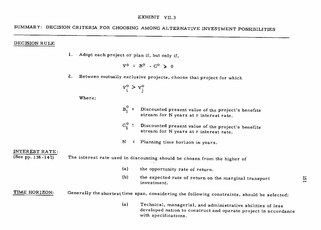
EXHIBIT VII. 3
SUMMARY: DECISION CRITERIA FOR CHOOSING AMONG ALTERNATIVE INVESTMENT POSSIBILITIES
DECISION RULE
1. Adopt each project 6r plan if, but only if,
° V = B° -C ° > 0
2. Between mutually exclusive projects, choose that project for which
V 0 > V?1 J
Where:
* Discounted present value of the project's benefits stream for N years at r interest rate.
00 Discounted present value of the project's benefits stream for N years at r interest rate.
N = Planning time horizon in years.
INTEREST RATE: (See pp. 138 -'141) The interest rate used in discounting should be chosen from the higher of
(a) the opportunity rate of return.
(b) the expected rate of return on the marginal transport investment.
TIME HORIZON: Generally the shortest time span, considering the following constraints, should be selected:
(a) Technical, managerial, and administrative abilities of less developed nation to construct and operate project in accordance with specifications.
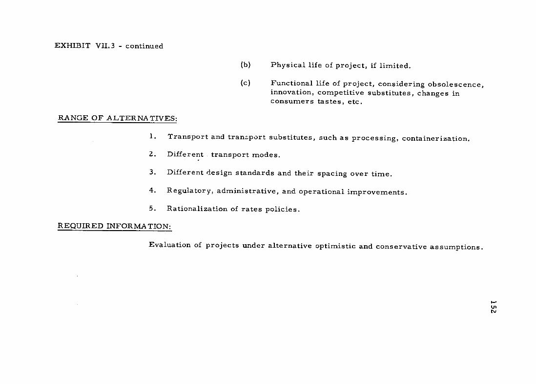
EXHIBIT VII.3 - continued
(b) Physical life of project, if limited.
(c) Functional life of project, considering obsolescence, innovation, competitive substitutes, changes in consumers tastes, etc.
RANGE OF ALTERNATIVES:
1. Transport and transport substitutes, such as processing, containerization.
2. Different . transport modes.
3. Different design standards and their spacing over time.
4. Regulatory, administrative, and operational improvements.
5. Rationalization of rates policies.
REQUIRED INFORMATION:
Evaluation of projects under alternative optimistic and conservative assumptions.
U11N~

PART II
CRITIQUE OF TRANSPORT
PLANNING PRACTICES
by
Tillo E. Kuhn

153
CHAPTER VIII
ANALYSIS OF PRE-INVESTMENT STUDIES_/
/ This analysis is based on work done by Tillo E. Kuhn, Clell G. Harral,
GraceW. Finne,andEleanorB. Steinberg. Mrs. Steinberg's draft is here
used in extenso.
This analysis of pre-investment studies completed in recent years
under the sponsorship of the major aid-giving agencies is concerned chiefly
with weaknesses in previous studies. No attempt is made to "second
guess" the recommendation of any study; instead the focus is on techniques
of analysis and their inadequacies.
The authors of many of the studies analyzed are fully aware of the
weaknesses of presently accepted techniques; indeed in some case the
suggestion to use the study came from them. Because examples do not
fairly represent the studies in their entirety, most references have been
deliberately obscured to avoid their identification.
Eighty-one reports concerned with economic development problems
of nearly forty countries were reviewed. Most of the studies were made
by private economic or engineering consulting firms under contract with
the various aid agencies, although some of the reports were written by
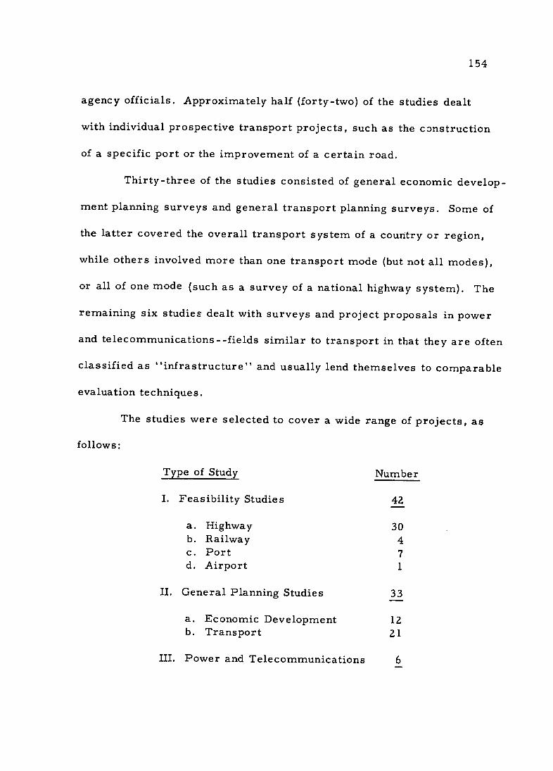
154
agency officials. Approximately half (forty-two) of the studies dealt
with individual prospective transport projects, such as the construction
of a specific port or the improvement of a certain road.
Thirty-three of the studies consisted of general economic develop
ment planning surveys and general transport planning surveys. Some of
the latter covered the overall transport system of a country or region,
while others involved more than one transport mode (but not all modes),
or all of one mode (such as a survey of a national highway system). The
remaining six studies dealt with surveys and project proposals in power
and telecommunications--fields similar to transport in that they are often
classified as "infrastructure'' and usually lend themselves to comparable
evaluation techniques.
The studies were selected to cover a wide range of projects, as
follows:
Type of Study Number
I. Feasibility Studies 42
a. Highway 30 b. Railway 4 c. Port 7 d. Airport 1
II. General Planning Studies 33
a. Economic Development 12 b. Transport 21
III. Power and Telecommunications 6

155
Of the eighty-one studies, twenty-seven were sponsored by the
Agency for International Development (AID), or its predecessor agencies,
and thirty-one by the International Bank for Reconstruction and Develop
ment (IBRD or World Bank). The remaining twenty-three reports had
various sponsorships, including some governments of developing countries.
Only one of the twenty-three was privately sponsored.
The research team reviewedtwenty of the eighty-one studies in
great deta".1, in accordance with an established survey format. (See
Exhibit I at the end of this chapter). The survey format is essentially a
list of key questions which an official of an aid-giving agency would want
answered by a pre-investment study. If all of the questions were answered
fully, a study would then be regarded as highly satisfactory. Since highway
development projects were more numerous than other types of transport
projects, the format was drawn up with particular regard to the problems
of highways, but, in general, it is applicable to all transport and other
infrastructure projects.
These twenty studies constituted the primary basis for this
chapter, and nearly all of the examples cited are drawn from them. The
remaining sixty-one studies, although read in entirety, were reviewed
only in terms of Part I of the format. Although these studies were
analyzed in less detail than the others, the research team felt that their
156
conclusions concerning the twenty were definitely corroborated by their
review of the other sixty-one.
THE ROLE OF PRE-INVESTMENT STUDIES IN PROJECT APPRAISAL
A potential transport investment goes through many stages of
project preparation and evaluation before a decision is reached as to
possible financing and execution. These steps are not always the same
for all projects and vary greatly among the various aid agencies.
Project Preparation and Evaluation in IBRD
Any classification of the steps involved in project preparation and
evaluation at the World Bank must be somewhat arbitrary because no two
loans are handled in precisely the same way. However, the basic phases
can be outlined roughly as follows: (1) loan application or request; (2)
preliminary or reconnaissance report; (3) detailed consultant report; (4)
final appraisal report.
Reconnaissance Report. A reconnaissance study is frequently a
brief and usually a low-cost report, the product of a short field trip by
outside consultants or agency officials to assess a project on a preliminary
basis. After receiving a request from a member country to consider a loan
for a given project, the IBRD generally sends a reconnaissance mission
to the field to prepare a report for internal use. This reconnaissance
report, which typically focuses almost entirely on the economic aspects
157
of a proposed project, is often the basis for a decision by IBRD to "go
ahead" with a project in existing form, to recommend changes in the
project, or to shelve a project temporarily or indefinitely.
Consultant Report. The World Bank sometimes, but not always,
engages private consulting firms to undertake economic and engineering
studies for prospective loan projects. Broadly speaking, those consultant
reports focusing on the economic aspects of a project deal with the antici
pated effects of the project on the economy of the country in question.
Engineering studies are concerned primarily with engineering specifi
cations and costs of the projects. (These studies are counterparts of the
"feasibility study" in AID project preparation procedures.) The main
points and principal findings of the consultant reports are generally in
cluded in the IBRD "appraisal reports." However, if a private consulting
firm is not hired and the work is undertaken principally by IBRD officials,
this entire phase is merged into the appraisal report stage.
Appraisal Report. The appraisal report, the final report in the
World Bank project preparation process, includes the principal findings of
the economic, financial, and engineering studies of a specific project.
Frequently a very detailed report, it is prepared by the staff of the Technical
Operations Department. Each division of the department is responsible for
the preparation of reports in a specific field. The transport division

158
prepares reports on roads, railroads, ports and waterways with the help
of engineers, economis-ts, financial specialists and other technicians who
specialize in a certain mode of transportation. The appraisal report is
addressed to the President of the World Bank, who presents it, together
with his own comments and recommendations, to the Board of Directors.
The recommendations are nearly always positive and invariably result in
the granting of a project loan. The reconnaissance stage is normally the
point at which a project is rejected if it is going to be.
Project Preparation and Evaluation in AID
The basis steps in the project preparation and evaluation process
in AID are: (1) "field generation;" (2) detailed feasibility study; (3)
loan approval.
The idea for a project is typically generated in the field by AID
officials stationed in a particular country or, in some cases, by the host
government. If the idea for the proposed projectis favorably received in
Washington, the next step usually has been a feasibility study. In the past,
a preliminary or reconnaissance type of report was not made by AID prior
to the feasibility study. Recently, however, the reconnaissance report has
begun to be incorporated into the agency's process for project analysis.
The lack of reconnaissance studies has been a weakness in AID
procedures in the past, and this in turn has often contributed to the weakness
159
of many feasibility studies. Because of the preliminary character of
these studies they have a certain neutral "no obligation" tone, and there
by offer an opportunity for rejecting or postponing a potential project
before the hopes of the host country are raised too high and before the
agency has become so involved that it feels committed.
Feasibility Study. The feasibility study is the basic source of infor
mation in AID pre-investment project analysis. The Foreign Assistance
Act of 1961, Section 611, requires a technical and economic feasibility
study for all capital projects in excess of $100,000 to receive U.S. fi
nancing under the provisions of the Act. / To implement this provision,
_/ Legislation on Foreign Relations with Explanatory Notes, Joint
Committee Print, Publication No. 93389, 88 Cong. 1 sess. (March 1963),
pp. 30-31.
consulting firms under contract with AID have been advised to prepare
their reports along the guidelines sec forth in the AID manual entitled,
Feasibility Studies, Economic and Technical Soundness Analysis, Capital
Projects. /
/ Issued June 1, 1962, and revised September 1, 3963.
The feasibility study is similar to the consultant reports described
earlier under IBRD procedures. The end result is intended to be a

160
determination of the economic and technical "feasibility" or "desirability"
of the proposed project. Frequently, the feasibility study is the first
formalized report in the preparation of a project. For example, an AID
loan of over $7 million to a South American country, which was announced
in August 1963, for the improvement of three roads and a bridge was based
on feasibility studies without any prior reports.
Loan Approval. The final stage in AID procedures is that of loan
approval. This is an administrative procedure in which the loan is either
disapproved or approved, theoretically on the basis of the feasibility study.
Although the recommendations of virtually every feasibility study are
positive, the loan is not approved in every case.
Cost of Pre-Investment Studies
The most important factor determining the cost of a pre-investment
study is the amount of engineering involved. As a result, there is a wide
variation in the outlays for diffr#-rent types of studies.
A recent reconnaissance study sponsored by AID that involved no
engineering cost only $31,000. The contract paid for two economists each
working two man-months in the field, local technicians and secretarial help,
and one man-month for each of the two economists to complete the report
in the home office. The $31,000 also covered the cost of reproducing fifty
copies of the report and a fixed fee for the contractor.

161
By contrast, an economic and technical feasibility study which
included preliminary engineering for the improvement of an 85-mile high
way was estimated to cost $150,000 and required about six months to
complete. /
_/ Foreign Assistance Act of 1963, Hearings before the Committee on
Foreign Affairs, House of Representatives, on H.R. 5490, 88 Cong. 1 sess.
(1963), p. 264.
AID funds obligated for a feasibility study of a bridge, including
studies and cost estimates of connecting roads, amounted to $250,000 for
a six-month study, _/ while an economic and engineering feasibility study
/ Ibid., p. 258.
for a proposed 957-kilometer road, including preliminary engineering and
with a four-months time constraint, cost $900,000.
A complex economic and technical feasibility report dealing with
the siltation problem of a port and the feasibility of locating an alternate
port in another city was sponsored by the United Nations Special Fund,
with IBRD as executive agent. The study was completed in one year at a
total cost of $1,365,000, of which the Special Fund paid $1,015,000 and the
host government the equivalent of $350,000. _/ Special Fund financing calls
_/ United Nations Special Fund, Report 1963: Target: An Expanding
162
World Economy, p. 44.
for at least partial matching by the host government, a practice which is
not normally followed by other aid agencies.
TERMS OF REFER] NCE FOR PRE-INVESTMENT STUDIES
The terms of reference for pre-investment studies are essentially
instructions to consultants with regard to data which should be obtained
through field investigations and the desired analysis of the data. The terms
of reference are normally included in the contract between the aid institu
tion and the consultants and are frequently included, in full or in summary,
in the final report.
The terms of reference are very important because they affect the
orientation of the consultants and determine the framework of the report.
In some cases, the terms of reference are extremely detailed; in others,
they are short and not very specific. However, the terms of reference for
AID surveys are often written in such a manner as to influence the con
clusions of the final report. In numerous reports, it appeared that the
aid institution had already determined to build a certain road or rehabili
tate a railroad (perhaps for political reasons) and regarded the consultants'
report as merely a means of justifying the project in question.
It should be noted that there is a difference between project justi
fication and project appraisal. When an aid agency has already, in fact,
committed itself to a project before the investment analyses are made, it
163
is generally felt by agency officials that the conclusions of the studies
are not supposed to be negative with regard to the project loan, and the
task of consultants becomes that of presenting a rationale for the project.
Project appraisal, on the other hand, implies a genuine economic
analysis of the project. Its conclusions about the economic desirability
of implementing a proposed project may be either favorable or unfavor
able. There is always good re, son for honest appraisal even in situations
where the final result is predetermined because only the appraisal can
reveal the economic costs of pre-determined objectives. Unfortunately,
project justification and project appraisal in practice are often intertwined,
and a positive bias in the terms of reference is frequently found in AID
sponsored studies. An illustration of terms of reference with an inherent
but perhaps unintended positive bias may be found in those drawn up for
a port feasibility study:
"Conduct such studies, investigations and surveys as may be necessary to determine and recommend a technically sound and economically feasible long-range general plan for the development of the port area.
"The construction increment which is recommended for initial implementation shall be so planned so as to afford a port facility which will most efficiently and economically serve present and reasonably projected traffic." [Italics ours.]
To render a more objective flavor, these terms of reference might
have been written as follows:
"Conduct such studies, investigations and surveys as may be necessary to determine whether or not it may be
164
technically or economically sound" etc. and to conclude "if construction is not deemed advisable at the present time, state what other measures may be initiated so as to afford an operable port facility which will most efficiently and economically serve present and reasonably projected traffic."
In the past two or three years, AID has initiated a limited number
of reconnaissance studies. In some cases, the terms of reference for
the consultants undertaking these missions have been less biased in tone
and far more complete than those for most feasibility studies. In 1963,
AID contracted for-a reconnaissance study of a proposed road project in
Africa. The consultants were requested to investigate the economic
benefits of the road, which was to constitute "Phase I" of the reconnaissance.
If the economic report proved favorable, "Phase II," or the engineering
side of the project, was to be covered by a subsequent mission. The text
of the terms of reference for the "Phase I" consultants are shown in
Exhibit II at the end of this chapter. Briefly, the terms of reference for
this project covered the following major topics: (1) effect on development
in project area; (2) position of project in overall program; (3) relation to
other transport systems; (4) anticipated economic benefits; (5) present and
future traffic generating activities; (6) traffic capacities; (7) justification
of the scope of improvement; (8) indigenous capabilities.
The very comprehensive terms of reference resulted in an
equally comprehensive report in which the consultants took the intiative

165
to go beyond the actual wording of the terms of reference and suggest an
alternate route for part of the project. Such an alternate solution might
have been incorporated in the original terms of reference under Section I,
"Effect on Development in Project Area," by inserting "(d) if an alternate
route for the road or part thereof seems more beneficial to the development
of the area, include the alternative solution and state reasons why.
preferable.
It may be questioned, however, whether a project can be evaluated
without taking the estimated investment into account. Benefits must be
considered in relation to costs, and even with preliminary cost figures,
the conclusions of a study may require further engineering findings. Local
construction costs per mile in similar terrain and bridge construction costs
per foot of bridges with similar spans may be used as rough estimates, and
the terms of reference should have required such preliminary cost estimates,
with an estimate as to the probable range of error.
THE PROJECT IN RELATION TO THE ECONOMY
After the terms of reference, or purposes, are set forth, the next
section of a pre-investment study is usually a description of the economy of
the country. The major weakness of this phase of pre-investment studies
tends to be a failure to relate the general economic information to the
proposed project.

166
One highway feasibility report from a developing country included
fifty-two pages of general economic and geographic data covering location
and external connections, terrain and soils, geology, climate, water supply,
natural vegetation, population, education, labor force, agriculture and
forestry, mineral resources, energy resources, industry, foreign trade,
and national financial position. This extensive coverage, however, was
poorly integrated with the analysis of the road project. While the economic
analysis pointed out the importance of a major crop to the economy, there
was no discussion of the current marketing practices of this main crop
and how the road project might affect them.
In another feasibility study of a road project, twenty-three pages
were devoted to general economic analysis and to the importance of highway
transport in the economy. Included were such subjects as location,
physical features, economic features, geology, meteorology and hydrology,
temperature and wind, gross national product, principal commodities,
technical skills, land values, truck transport profits and road accidents.
Additional economic information was brought into the report in the form
of interviews with government officials. None of this information was
specifically related to the proposed project. In addition, the amount and
nature of other investments contemplated for the area affected by the
road project were not covered.

167
In contrast to the extensive coverage in the reports cited, another
feasibility report on a highway project stated that the economic information
for the area covered was too voluminous to be included in detail in the
report; consequently, the general economic coverage was confined to
one paragraph.
In sharp contrast to these typical examples is a study for a
comprehensive highway program for a country in Central America, where
a comparatively successful effort was made to relate the proposed high
way system to the national economy. The entire study and its recom
mendations were derived from the development potential of the country
and the policy goals of the government. Not only were detailed population
and other data included by region and by type of economic activity, but
the information was made the basis for transport planning and traffic
forecasts. Other studies also presented demographic information (although
rarely in such detail), but the difference between these studies and the
Central American study was that the latter actually used the population
projections in order to project domestic food requirements. The
remainder was assumed to be available for export, and this information
was in turn used in determining transport requirements.
THE PROJECT IN RELATION TO OTHER TRANSPORT FACILITIES
The major reason for relating a proposed project to existing
regional transport facilities is the possibility that what appears to be
168
optimal from a project standpoint may be less than optimal from a regional
standpoint. For example, one feasibility study for a road project dealt
exclusively with the proposed highway, and almost completely ignored the
effect of the new road on existing water, rail and air connections for the
same route. In a study for a highway project which involved an international
connection no discussion was included of other components of the inter
national connection and their implications. In contrast, another railway
study devoted an entire chapter to related problems of road transport.
Relating the proposed project to transport facilities outside the
region immediately affected by the new or improved facility is important
for two main reasons. First, there is the question of technical compati
bility of the new facility with connecting transport media. For example,
if a study concluded that a transport facility was required in province X
and that the most economical facility would be a road, consideration should
be given as to whether goods moving over the new road would, in order to
reach their final destination, have to be transshipped to an inland water
facility or to a railroad, thus involving costs not included in the initial
calculations.
Second, there is the problem of economic compatibility of the
proposed facility with other transport facilities outside the immediate
area of influence. In one overall transport study it was discovered that
169
a local marketing board had authorized a certain amount of the major
crop of the northern section of the country to be hauled to a southern port
by road. This traffic had previously been hauled by the national railway
system (which the report considered to be the low-cost carrier). The
diversion of export-traffic from rail to road resulted in the loss of a
considerable amount of the higher rated import traffic. Traffic diversion
resulting from a new facility in one region of a country can have conse
quences for the entire transport system.
INVESTMENT ANALYSIS: COSTS AND BENEFITS
Benefit-cost analysis was the principal technique for investment
analysis in the majority of the project-oriented studies. This technique
generally consists of adding up the estimated benefits and costs expected
to accrue from a proposed project. Only one of the studies made any
attempt to discount benefits or costs. (See the later section, "Other
Problems of Benefit-Cost Analysis.") A ratio of benefits over costs was
then computed. If the ratio was 1 or greater than 1, the results of the
investment analysis were considered positive; the project was considered
worthwhile and in many cases was undertaken by the aid agency which
financed the feasibility study.
The conceptual difficulties inherent in the benefit-cost technique
are dealt with in Part I of this volume. Since this technique was in fact
170
used in most of the pre-investment studiea, attention in this paper is focused
on chronic errors in benefit-cost calculations rather than on the method
itself. The line between theoretical and practical difficulties is not sharp,
however. Some of the errors of the benefit-cost calculations included in
the feasibility studies stemmed directly from conceptual difficulties.
In general, the outstanding weaknesses of the benefit-cost analysis
in the project studies were the overestimation of benefits and the equally
serious underestimation of costs. This meant that the benefit-cost ratio
in virtually every study turned out to be 1 or greater than 1. The consis
tently positive results of the investment analyses fit in very well with
the frequently positive bias of the terms of reference which was discussed
earlier. Here again, project appraisal and project justification were not
kept separate.
Problems in Measuring Benefits
Broadly speaking, all benefits which derive from transport projects
are in fact net increases in production of final goods and services. These
net increases in production come about in one or two of the following three
ways: (1) where there was no transport facility at all prior to the invest
ment in question, agricultural industrial or other types of production may
be stimulated by the new facility; (2) where there is an improvement of an
existing facility, new production may be stimulated by reduced costs or

171
increased capacity; (3) when an old facility is improved, there is also
a release of resources due to reduced costs which may be transferred to
other uses.
Defining Benefits. Although there are a number of conceptual
difficulties, the practical implications of which led to gross errors in
estimating benefits, special mention must be made of two frequently
recurring problems. Both of these problems derive from a failure to
define precisely the term "benefits"--to determine what should legiti
mately be counted in a benefit-cost analysis and what should not.
The first problem was failure to distinguish between financial
benefits and economic benefits. Briefly, financial benefits are those which
have a monetary value and which a banker or accountant would consider
when investigating a loan. These include, for example, revenues which
would accrue to a government from gasoline taxes generated by new or
improved road, or from port dues levied on users of a new port. It is
necessary for an aid agency to undertake a financial analysis of a specific
project (or of the national budget, if the project is not expected to be self
liquidating) in order to determine whether or not a loan will be repaid.
But this type of analysis should be kept entirely separate from the econo
mic feasibility study of a transport project, or any other developmental
project. The purpose of the economic as distinct from financial appraisal
172
is to allocate resources efficiently--to choose the right investments. The
primary concern should be the developmental impact of the investment.
The criterion to use in determining whether or not a particular item
should be counted as a benefit is whether it contributes to raising the
output of the economy.
One study of a road project provides an example of confusing the
economic with financial benefits. In this case, the only benefits which
the consultants used in the benefit-cost ratio were government revenues.
These included direct revenues generated from user taxes on vehicles,
tires, fuel, etc., plus indirect revenues computed as the percentage of
Gross National Product represented by highway transport multiplied by
total government revenues minus the direct transport taxes on vehicles,
fuel, tires, etc., mentioned above. A total annual anticipated tax receipt
per vehicle-mile was then multiplied by annual projected traffic estimates
in order to arrive at total tax revenues, or total benefits. A number of
traffic projections were made. One method involved estimating population
and GNP and correlating traffic growth with that of GNP. Another esti
mate was based on the assumption that the traffic growth on this particular
road would approximate the average traffic per square mile in the broad
geographical region within which the road would be located.
In this example, the estimation of benefits suffered from at least
three shortcomings: (1) The method of estimating the indirect tax
173
revenues was highly questionable. The existence of indirect tax revenues
was simply assumed. No specific levies of this type were mentioned, and
it is conceivable that there were no sources in indirect revenues. Further
more, there was no valid reason to assume that whatever indirect tax
receipts might have existed were equivalent to the proportion of GNP
comprised by highway transport. (2) Future traffic was not estimated
on the basis of projected increases in real output or on population shifts
which would result in part from the new transport facility. Instead
traffic estimates (like indirect tax receipts) were made on the basis
of aggregate projections, such as GNP and population. The correlation
of future traffic, future vehicle registrations, and other transport data
with projections for GNP or other national aggregate figures was a
common error found in pre-investment studies. This type of correla
tion is valid only for aggregate traffic projections and even then the rela
tionship cannot be assumed to be stable. (3) By taking government
revenues as the sole measure of benefits, emphasis was placed on the
financial merits of the project and no way was provided for integrating
the economic benefits into the benefit-cost analysis.
The second problem resulting from failure to define benefits
precisely concerns "indirect" benefits. In some studies, an attempt was
made to distinguish between direct and indirect benefits and to include both

174
categories in the benefit-cost calculations. Although there was no con
sensus as to what indirect benefits actually were, most of the studies
treated them according to one of two definitions: (1) Indirect benefits
are those "intangible" nonmarketed, and nonquantifiable benefits of a
social, political, or military character. (2) Indirect benefits are those
which accrue to others than users of the project.
Often, the intangible, nonquantified benefits were introduced to
increase the benefit side of the benefit-cost ratio and to insure a ratio
greater than unity. Sometimes these benefits were simply alluded to as
an additional argumeat on behalf of the proposed project. For example,
one study of a proposed road project included such questionable benefits
as general enhancement of road transport (this "benefit" could be obtained
from any project) and stimulation of tourism (although the resort area in
question was already connected with the national railroad system by a
hard-surfaced road). These alleged "benefits" although not quantified,
were regarded as sufficient to offset a higher cost of moving the potential
freight by the proposed road rather than by the existing railway.
The indirect benefits implied by the second definition- -benefits
to nonusers--are usually not legitimate benefits in that they almost in
variably involve double-counting. These benefits are typically the same
ones passed along from one person to another. In the same study of a road
project, the reductions in total operating costs were counted as a direct

175
benefit and increases in land value as an indirect benefit. This is, however,
the same benefit since savings in transport costs increase net profits in
agriculture which in turn raise land values; the transport operator's
benefit is being passed along to the farmer or land owner.
It is possible, however, that an investment will result in external
economies or diseconomies accruing to other sectors vhich should be
added to or subtracted from the other measured benefit,. Whether or
not there can be such externalities depends upon whether the project is
being analyzed from a national, regional, or strictly project point of view. /
/ See page 58.
Estimating Legitimate Benefits. The broad categories of benefits
which should be included in a benefit-cost calculation are: expected new
production, stimulated partly or entirely by a new or improved transport
facility, and resources released by reductions in costs of handling existing
traffic.
A major criticism of the pre-investment studies was that very few
of them attempted to estimate anticipated increases in real output. Some
studies undertaken for "penetration," "developmental" or feeder roads
failed to project estimates of increased agricultural production stimulated
by the proposed facility. Instead, the main emphasis was on reduced
operating costs to transport users--not only to present users in cases where
176
there was some sort of existing primitive road or track, but to future
users as well. In order to estimate savings to potential users of the
proposed facility, traffic forecasting was required. Thus, a central
feature of many of the studies was an analysis of current and future
demand for transport in the region to be served by the facility.
The method generally used in the surveys studied was, first, to
estimate savings in transport costs. Broadly speaking, a cost savings
estimate is computed by calculating reductions in wear and tear on
tires and vehicles, lower fuel costs, and reduced labor costs. / The
/ Savings in maintenance costs are omitted here. It should not be,
assumed that maintenance costs are lower on an improved road than on
an unimproved road.
savings are then compared with present operating costs. The savings
estimate was then applied to forecasts of average daily traffic, in order
to assess the benefits which could be expected from the new facility.
Average daily traffic figures, in many cases, were based on estimates
of growth in GNP and past traffic trends, instead of on projections of
increases in agricultural and industrial production in the region to be
served by the facility.
This technique of basing benefit estimates on reduced transport
operating costs, combined with traffic forecasts, was borrowed from the

177
United States and other developed countries. Such analysis is more
appropriate in the United States and Europe, where improvements to
existing highways generally involved benefits that accrue predominantly
to users of the facility. The technique is less applicable in the develop
ing countries, however, except in such cases as ports and urban roads
where traffic congestion is already a serious problem.
In rural areas of underdeveloped countries, however, it is frequently
a developmental or feeder road that is being studied for a region which
is presently served by no road, except possibly a track. The principal
benefits cannot be assessed in terms of savings to users since there are
few or no present users. Benefits must instead be assessed in terms of
the increases in real output which can be expected to result in part from
the new facility. In cases where a road of some sort exists with a small
amount of vehicle traffic, the main emphasis still must be on projections
of increases in production, although this should be supplemented by esti
mates of reduced operating costs to present users. In other words, the
primary beneficiaries will not be the present users in either case.
It should be noted that, after projections of increases in production
are made on a commodity-by-commodity basis, these estimates must
be translated into actual traffic forecasts in order to determine design
standards for the road and to estimate future maintenance costs.
178
Estimating Increases in Real Output. A study of a highway system
for a Central American country provided a rare exception to the absence
of forecasts of increases in real output and to the gross inadequacies of
traffic forecasts characteristic of most of the pre-investment studies.
In this study, agricultural production over the next few years on a
commodity -by-commodity basis was projected. The production projections
were then broken down according to amounts which would be consumed
locally and amounts which would be transported. Projections of output
in the forestry and manufacturing sectors of the economy were also
included. The quantities and kinds of commodities which would be pro
duced were, in turn, based on estimates of local food requirements,
population projections, estimates of future world demand for various
commondities, suitability of soil and climate to various crops, and ex
pected development of particular food processing and other manufacturing
plants. The output projections were then translated into traffic projections
which, along with extensive origin and destination survey data, were used
to determine road location and design standards.
Total projections of freight and passenger volumes for the 10
year period were ultimately used in the sample benefit-cost analysis.
Even here, many assumptions were required but the method was appro
priate.

179
The Attribution Problem. One of the knottier conceptual problems
arising in connection with estimating increases in real output in the so
called "attribution problem." One aspect of this problem is, briefly:
how much of the increase in real output associated with a given project,
such as a new highway, is attributable to the highway and how much to other
investments? If there is an increase in agricultural output on land near
the highway, this increase was stimulated not only by the new transpoTt
facility but also by certain investments in agriculture. In most of the
feasibility studies all of the increases in output were attributed entirely
to the new transport facility or a certain percentage was attributed on an
arbitrary basis. This practice, as well as that of counting unquantified
or illusory indirect benefits and financial (in addition to economic) bene
fits, helps to explain why the benefit side of the benefit-cost ratio was
frequently overstated.
A general transport survey for a developing country "solved"
the attribution riddle by counting as a highway benefit the full value of
projected increases in living standards. The consultants recommended
that, for each proposed road, the benefit calculation include the projected
increases in income for all families living within 10 miles of the road and
at the terminus, based on the monetary value of expected increases in the
marketable agricultural production of the families. It was assumed that
the full increase in agricultural production would be stimulated solely by

180
the road and that no other investments would be necessary to bring about
a rise in production or in farm income.
Occasionally, project analyses avoided this problem by correctly
considering a proposed road and associated development projects as one
package. In one road project feasibility study, the benefits of the proposed
roads were not separated from the estimated net income of the farms to
be served by the roads. The net farm income for a 15-year period was
estimated. Behind these estimates of the value of agricultural production
were a number of basic assumptions as to the rate of colonization, the
amount of marketable production, obtainable prices for agricultural
products, the foreign exchange rate and the relationship of gross sales
value to net income. The benefit analysis was one of "joint" benefits,
subsequently compared with the cost of the farm scheme plus the esti
mated cost of the roads.
Estimating Benefits in Terms of Cost Savings. An example of the
more typical method for estimating benefits found in the feasibility studies
is provided by a study of three roads in country. In this case,one
benefits were estimated on the basis of reduced operating costs. The
steps of the analysis were as follows:
1. Estimates were made of average operating costs for main
categories of vehicles on different types of roads. (Operating costs

181
included depreciation, repairs, fuel, lubrication, tires, and driver's salary.)
2. Weighted averages were calculated for vehicle operations on
unimproved roads and on paved roads. The savings on the proposed roads
were assumed to be identical with the difference of the two weighted
averages.
3. The estimated traffic on each proposed road as expressed in
number of vehicles per day (average daily traffic, or ADT) was reduced
by a factor derived from an estimate of how many vehicles would travel
the whole length of each road. How these average trip assumptions were
arrived at was not explained. The adjusted figures then represented the
number of vehicles traveling the full length of the road.
4. The estimated weighted savings per vehicle-kilometer for each
road were multiplied by the adjusted average daily traffic data and the
length of the respective roads, and projected on an annual basis for each
year of the 20-year forecast period. The assumption that the traffic
composition would remain the same over the 20-year period to justify
the use of the weighted average operating cost saving of the initial year
was explicitly stated. The assumption of identical trip lengths during the
20-year period was, however, not explicitly stated.
The classic problem of methodology illustrated by this example
is that the consultants applied the cost savings figures not only to existing
traffic but to additional future traffic as well. In this situation future

182
traffic estimates are used as substitutes for estimates of increases in real
production. This is an inadequate measure because estimates of savings on
traffic which did not exist before the road improvements do not necessarily
reflect the real benefit from new production. The factors which should be
taken into account are: (1) the amount of resources released by reductions
in operating costs; and (2) the amount of additional output generated in
part by the highway improvements.
Apart from this fundamental error, the study ran into trouble with
such problems as estimating average trip length and projection of traffic
composition over the next 20 years. On these matters, resort was made
to arbitrary assumptions as to average trip length, which, of course, yield
a wide range of annual vehicle utilization figures.
Absence of Stated Assumptions Underlying Projections: The matter
of using arbitrary assumptions as bases for projections of various kinds
leads directly to another persistent weakness in pre-investment studies as
a whole. This was failure to make explicit the assumptions on which pro
jections were based. Thus, in addition to depending on inadequate available
data, projections were further weakened by the fact that the users of the
studies could not follow the logic of methodology on which the projections
were made.
Other Methods of Calculating Benefits. Conceptually, the method
of estimating savings in terms of increased profits to truck operators is
183
very similar to that of making the calculation in terms of reduced trans
port rates. The basic difference between the two is that, in the case of
the former, the savings are retained by the transport operators; in the
latter, they are passed along to users.
The basic method used in determining this type of savings was:
(1) to estimate what either the profits or rates would be after the road
improvement was made; (2) to multiply this figure by a projected annual
average traffic estimate. In virtually every study in which this kind of
calculation was made, assumptions as to present rates or profits, future
rates or profits, average length of haul, and average annual traffic were
made on an essentially arbitrary basis. Very often, the bases for the
assumptions were not elucidated.
Calculations of reduced rates or profit increases are not usually
good benefit indicators. In the first place, whether the savings are retained
by the transport operators or passed along to the users depends in large
measure on the degree of transport monopoly or competition involved. If
the situation is one of total monopoly or near monopoly, the truckers are
likely to retain the savings as profits. If there is considerable transport
competition, the saving may well be translated into lower rates. The pro
blem here is that, in the latter case, it is very difficult to know whether or
not all of the savings were in fact translated into lower rates. Furthermore,
in cases where there are few or no effective restrictions on entry of new
184
trucking firms, it is hard to know whether the lower rates result from
lower operating costs or from an increased supply of trucks in relation
to freight offered.
Whether cost savings are retained as profits or passed along as
rate reduction,, the main point is that an estimate must be made of the
effects that the savings will have on economic development.
A Special Case: A New Highway Parallel to a Railway. Occasionally,
a pre-investment study of a proposed highway to be built parallel to Zn
existing railroad is undertaken. In such cases, the savings benefit is
estimated by comparing the projected operating costs of the highway with
the present operating costs of the railway. Although such a comparison is
theoretically conceivable, it is extremely difficult and complicated to carry
out in practice. In order for the comparison to be valid, it is necessary,
for example, to evaluate whether or not the present rail costs are "true
costs"; existing rail rates cannot automatically be accepted as valid basis
for comparison.
In one road feasibility study the relative benefits of the proposed
highway were estimated as the difference between direct operating costs
of providing services on the new highway and continuing to rely on rail
service with various improvements. Certain variations of the two basic
solutions were also compared.
185
A "freight benefit" was calculated as the difference in total
operating costs of the two facilities. (The present rail costs were taken
as given.) The result came out negatively for the road; the railroad solution
was given the comparative advantage.
Subsequently, highway passenger benefits were computed at "about
20 percent of direct operating expenses by highway," which elsewhere in
the report was estimated for heavy truck trailers. The relationship
stipulated between the operating costs of passenger vehicles and truck
trailers was not in any way ,ubstantiated. The passenger "benefit" per
mile turned out, not surprisingly, to be the highest for the longest route,
since it was based on a kilometer cost rate. No passenger benefit was
computed for the railway solution, but the positive "road passenger benefit"
was added to the negative road "freight benefit" to get a slim positive road
benefit, termed "irnputed benefit."
Nonmonetized Cost Reductions. Among the mo-e serious errors
in calculating benefits resulting from cost savings was that of attempting
to assign values to nonmonetized cost reductions, such as time savings
and accident reduction. In specific cases it may be possible to assign an
accurate monetary value to savings resulting from reduced accidents or
wage costs whtn transit times are reduced. In some of the studies, how
ever, these categories were useii to improve the benefit-cost ratio without
evidence that the savings did exist.

186
Problems of Cost Calculations
As indicated earlier in this paper, the main weakness in estimating
costs was underestimation. In only a few cases was it possible to find
both original cost estimates and final costs for projects which involved
construction. / In case one (highway construction), the original estimate
/ Most of the loans by U.S. aid agencies, until the last three or four
years, were for transport equipment only, and not for construction of
new or improved facilities. While a number of transport development
loans involving construction have been made in the 1960's, these projects
are not yet completed, so that it is impossible to obtain final cost
figures. (Estimates for equipment costs, are, of course, quite straight
forward.)
was $16 million and the final cost $27.4 million; in case two (highway
construction), the figures were $19.5 million and $47 million; for case
three (airport improvements), $1.5 million and $2.7 million; for case
four (highway construction, $5.3 million and $8.0 million. (In the last
example, the figures covered only the foreign exchange costs of the
project.)
Omission of Cost Items. This chronic underestimation of the
actual monetary costs was attributable mainly to the fact that in nearly
every study, important cost items were omitted from the cost estimates.

187
One of the chief omissions was maintenance costs. For example, one study
presented estimates of the costs of construction of maintenance stations
and repair shops and of the equipment needed for these shops, but it
completely omitted these estimates from the benefit-cost analysis.
Although rough estimates of maintenance costs over the first five years
(instead of for the assumed life of the road) were included, the estimates
were unsubstantiated and were much lower than per-kilometer mainten
ance costs for roads in a nearby country. Other omissions included
"system costs," such as feeder roads and vehicles which have to be
imported, and labor and administrative costs.
Not only were the monetary costs underestimated in the majority
of the reports but the full economic costs were also usually underestimated.
The attribution problem discussed earlier in regard to estim2ting benefits
resulting from increases in real output arises again in connection with
estimating costs. Many studies counted all or a large percentage of
increases in output (agricultural output, for example'i as a benefit attri
butable to the new transport facility. However, they seldom included the
additional costs of increasing output--such as fertilizer, new farm
machinery, or the services of agronomists and soil scientists--on the
cost side of the calculations.
A common weakness in the cost estimates which may or may
not contribute to the underestimation of costs, but certainly detracts
188
from the practical usefulness of the estimates, was failure to present
costs in terms of quantities and unit prices. Instead, cost figures were
commonly presented only in terms of the final figure, with no item-by
item breakdown. In some cases, the source of price quotations was not
indicated. In one study, for example, prices appeared to be factory prices
in the United States, rather than F.O.B. prices in the port of entry of the
country for which the project was planned.
Overemphasis on Engineering and Cost Calculations. While the
benefit side of the benefit-cost calculation is largely derived from
economic analysis, the cost side is essentially based on engineering
studies. One of the major weaknesses of the pre-investment studies
was the lack of balance between the economic and engineering sections.
In many studies, much more of the report was devoted to the engineering,
or costs, aspects than to the economic analysis.
The reason for this is, possibly, that engineering techniques are
more developed and straightforward than those of economics. If the
reconnaissance study became an established part of project evaluation
procedures, a good deal of the costly engineering studies could be eliminated.
This preliminary report focuses on the economic aspects of a project, and
a rough estimate of costs is all that is needed. Only those projects for
which the reconnaissance reports came out with favorable recommenda
tions would require an extensive engineering study.
189
Other Problems of Benefit-Cost Analysis
In estimating benefits and costs, two quesions invariably arise:
What time period should be used in estimating the benefits--that is,
how long will the benefit be expected to last? Over what time period
will the costs be incurred? These questions were ignored in many of the
studies. Occasionally, an arbitrary life expectancy of the transport facility
was assumed, and, also occasionally, a rate of interest (usually the interest
rate set by the loan agreement with the loan agency) was assumed. In
only one case was the assumed time horizon and interest rate explained
or selected on any particular basis. Yet, obviously, these two factors are
essential to the economic evaluation of a project and alternative project
possibilities.
One last weakness in the benefit-cost calculations in most of the
pre-investment studies was the fact that they were expressed in terms
of a ratio rather than in terms of a "gap" or difference between benefits
and costs. Some items could well. be considered as either a negative cost
or a positive benefit (such as reduced maintenance), and how they are in
troduced into the fraction can have a substantial effect in the final ratio
but no effect in a measurement of the difference or gap between benefits
and costs. Finally, a ratio is not as meaningful as an absolute value
figure. /
_ See page 123.
190
CONC LUSIONS
The deficiencies of the present system of evaluating proposed
transport projects are outlined below.
1. Project Justification
Many of the transport studies sponsored by AID in effect seek
justifications of predetermined decisions as opposed to "evaluations" of
meaningful alternatives. The former attempts to justify a particular pro
posal, ordinarily by demonstrating that benefits, measurable and non
measurable, exceed costs, that the ratio of benefits to costs exceeds
unity. The latter seeks to choose a preferred plan from a range of feasible
alternatives by evaluation and comparison in terms of specified objectives.
In addition to estimating the benefits and costs expected from each individual
project, good project evaluation answers two questions: "Why do anything?"
and "Why this way?" The project justification criteria provide only
necessary but not sufficient conditions for choosing projects and are in
adequate for economic planning.
Of course there are various factors, such as legal obligations and
past political commitments which can in fact predetermine certain projects.
In these cases, the need for evaluating alternatives is less clear, although
it can still be useful as an economic costing of political objectives.
However, there can be no excuse for a narrowly conceived and poorly
executed "project justification" for those projects to be assessed solely

191
or largely on the basis of their expected contribution to economic develop
ment or other specified objectives.
Fundamental deficiencies in the overall approach to project
planning which originate in a bias toward project justification include the
following:
a. Failure to carry out effective pre-appraisal.. AID currently
does not sponsor effective reconnaissance or pre-appraisal studies as a
routine procedure in the sequence of steps by which projects are appraised.
But it is very difficult for the agency to refuse support to a project once it
has mounted a major research study of the scale of its present feasibility
studies. In practice the agency often becomes committed to a project
when it agrees to a feasibility study, and any opportunity to influence the
decision at hand, in detail or in substance, is lost.
Furthermore, present feasibility studies encompass large inputs
of preliminary engineering design work. This expensive work cannot and
need not be undertaken for a wide range of alternatives.
Thus, the agency is reluctant to undertake a feasibility study until
its own staff is convinced by their analysis that AID should finance the
proposed project. However, the agency does not have the specialized and
expert staff that can independently accomplish an effective appraisal of the
complex range of technical alternatives for almost any given transport
proposal. The result is that one particular alternative (or limited number
192
of alternatives) is "locked in" as the project at a premature stage. Often
the only thing left for the expert consultants to do, as one disappointed
official remarked, is to provide "a good study to justify a bad decision."
b. Narrowly defined study specifications. The contract specifications
or terms of reference for the feasibility studies reviewed were often
written in such a way as to limit the range of alternatives narrowly. More
over, the wording of the specifications was often favorably biased toward
the proposed project.
c. Biased format of the decision criterion. The decision criterion
which AID specifies is that benefits of the project exceed costs over time.
That this, and those more advanced variations of the benefit-cost ratio
approach, constitutes a defective criterion was demonstrated several years
ago in discussions of water resource development. / There are many
/ J. Hirshliefer, J. G. DeHaven, J.W. Milliman, Water Supply: Economics,
Technology and Policy (University of Chicago Press, 1960), Chapters VI
and VII.
projects which satisfy this criterion which cannot satisfy other economic
and social criteria.
Furthermore) the study revealed evidence of a strong tendency in
practice to underestimate ultimate project costs and to overestimate
probable economic benefits. The net effect, of course, is to reflect a
favorable bias toward the particular project proposed.
193
2. Failure to Relate Proposed Project to the Economy
Undoubtedly due in part to the justification-oriented framework
within which the studies took place, a characteristic of the feasibility
studies reviewed was the lack of depth and perfunctory nature of the
"economic analysis," in marked contrast to the specificity and detail of
the average engineering analysis.
Frequently compiling available statistics for the country as a
whole was substituted for marshalling logic and evidence to provide a for
mal case in support of the project. The arguments relating the given
statistics to the proposed project were often naive or omitted altogether.
There were few attempts to relate the proposed project to the overall
transport network and to the natural resources, agriculture, industry, and
private as well as public investment plans of the economy. Under these
circumstances, efforts to determine the effects of the proposed invest
ment and to compute its benefits were necessarily less than satisfactory.
3. Underestimation of Project Costs
While the current study was not able to investigate the matter in
detail, underestimation of actual costs of construction was found to be a
common characteristic of pre-investment studies. This occurred despite
the detailed and expensive engineering reports in the studies.
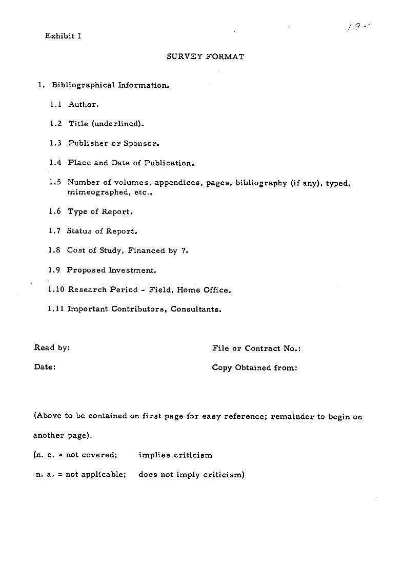
Exhibit I
SURVEY FORMAT
1. Bibliographical Information.
1.1 Author.
1.2 Title (underlined).
1.3 Publisher or Sponsor.
1.4 Place and Date of Publication.
1.5 Number of volumes, appendices, pages, bibliography (if any), typed, mimeographed, etc..
1.6 Type of Report.
1.7 Status of Report.
1.8 Cost of Study, Financed by ?.
1.9 Proposed Investment.
1.10 Research Period - Field, Home Office.
1.11 Important Contributors, Consultants.
Read by: File or Contract No.:
Date: Copy Obtained from:
(Above to be contained on first page for easy reference; remainder to begin on
another page).
(n. c. = not covered; implies criticism
n. a. = not applicable; does not imply criticism)

Exhibit I /9 )
2. Related Reports (list exact references).
2.1 Studies directly related to project, including preceding and succeeding reports.
2.2 Background studies taken into account.
2.3 Other references, research of interest; reviews, criticisms.
3. Data of Interest:
a) Typical road (rail, harbor, runway, etc.) construction and maintenance costs, in $ per mile or km., specify gravel or paved, number of lanes or tracks, possibly type of terrain; exclude major structures.
b) Typical freight rates (rail, air, road, water) in $ per ton-mile or ton-km.
c) Typical passenger rates, $ per passenger-mile or pass.-km.
d) Load factors, utilization factors of trucks, buses, etc.
e) Typical traffic volumes (in ADT =
average daily traffic); specify proportion of trucks, buses, autos.
f) Other data of interest.
4. Identification of Policy Objectives, Teerms of Reference, Instructions, Constraint., Prior Commitments.
4.1 Specified by Developing Nation.
4.2 Specified by Sponsor.
5. The Study in Relation to the Whole Economy, the Social, Political, Institutional Environment, National Development Plan.
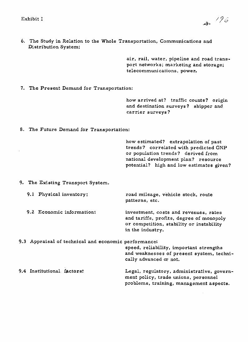
/9Exhibit I A-¢
6. The Study in Relation to the Whole Transportation, Communications and Distribution System:
air, rail, water, pipeline and road transport networks; marketing and storage; telecommunications, power.
7. The Present Demand for Transportation:
how arrived at? traffic counts? origin and destination surveys? shipper and carrier surveys?
8. The Future Demand for Transportation:
how estimated? extrapolation of past trends? correlated with predicted GNP or population trends? derived from national development plan? resource potential? high and low estimates given?
9. The Existing Transport System.
9.1 Physical inventory: road mileage, vehicle stock, route patterns, etc.
9.2 Economic information: investment, costs and revenues, rates and tariffs, profits, degree of monopoly or competition, stability or instability
in the industry.
9.3 Appraisal of technical and economic performance: speed, reliability, important strengths and weaknesses of present system, technically advanced or not.
9.4 Institutional. fx.ctors.e. Legal, regulatory, administrative, government policy, trade unions, personnel problems, training, management aspects.

Exhibit I
10. The Proposed Future Transport System and its Costs.
10.1 Physical description:
10.2 Engineering cost estimates:
10.3 Consideration of alternatives:
how much detail? where do technical standards come from? are technical alternatives considered?
how inclusive? are capital investment as well as maintenance and operating costs included? are roads as well as vehicles, airports as well as aircraft, etc. considered? are complementary investments taken into account, for example highway as well as warehouses and harbour costs? are high and low estimates given? is derivation of engi
neering cost estimates, from quantities and unit costs, shown? general documentation and technical support for cost estimates good?
Are alternative project proposals, involving different locations, different technical solutions, different time patterns and sequences, different engineering standards, considered?
10.4 Final technical recommendations: are they firm? well supported by analysis and technical evidence? can they be followed without further study by sponsors of study and developing nation?
11. Benefits:
how estimated? documentation? technical and economic evidence? what categories are included in benefits? monetary? role of user taxes in benefit assessment? non-monetary? vehicle operating cost savings? broad national benefits? social, political, etc. aspects?
12. Investment Analysis.
12.1 Identify investment methodology and criteria used: benefit-cost ratio? maximization of net benefits? other?
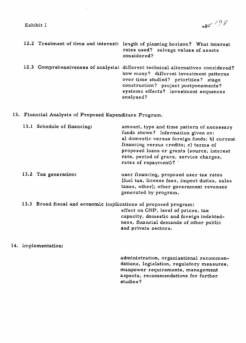
Exhibit I
12.2 Treatment of time and interest:
12.3 Comprehensiveness of analysis:
length of planning horizon? What interest rates used? salvage values of assets considered?
different technical alternatives considered? how many? different investment patterns over time studied? priorities? stage construction? project postponements? systems effects? investment sequences analysed?
13. Financial Analysis of Proposed Expenditure Program.
13.1 Schedule of financing:
13.2 Tax generation:
amount, type and time pattern of necessary funds shown? Information given on: a) domestic versus foreign funds; b) current financing versus credits; c) terms of proposed loans or grants (source, interest rate, period of grace, service charges, rates of repayment)?
user financing, proposed user tax rates (fuel tax, license fees, import duties, sales taxes, other); other government revenues generated by program.
13.3 Broad fiscal and economic implications of proposed program: effect on GNP, level of prices, tax capacity, domestic and foreign indebtedness, financial demands of other public and private sectors.
14. Implementation:
administration, organizational recommendations, legislation, regulatory measures, manpower requirements, management aspects, recommendations for further studies ?

Exhibit I ,.6 . ,
15.. Evaluation of Report.
15.1 Balance: between engineering and economics? data collection and analysis? past and future? analysis and action recommendations?
15.2 Does it follow current AID Manual?
15.3 Outstanding strengths and weaknesses: in field work? methodology? documentation? engineering aspects? economic analysis? benefit assessment? cost estimates? transport demand forecasting? investment analysis? financial analysis? choices put forward? action recommendations? implementation?
15.4 General assessment of study: complete? honest? excellent? very good? good? mediocre? poor? very poor? If you were the decision-maker, would you invest money on the basis of the evidence presented in the report?

Exhibit II
Terms of Reference for East African Road Project
"With the objective of ascertaining the economic feasibility of the proposed "X" road, the Contractor will (a) place emphasis on the collection of data an(, evaluation of economic conditions and potential of the areas to be served by the proposed route; (b)assess the proposed route and the natural segments of the route in terms of national development prospects taking full account of all communication facilities under construction or planned; and (c) provide the degree of analysis and evaluation of the foregoing which will produce monetary benefits to "Y" for segments of the route."
After a section on cooperation with the local authorities and the
local AID mission, the terms of reference continue:
"In performing the economic feasibility survey the Contractor shall develop the following information:
1. Effect on Development in Project Area
(a) General description of the area to be served by the proposed "X" road (physical and economic geography, including agriculture, processing, manufacturing, centers of population, topography, geology, vegetative cover, and climate as related to traffic generating economic activity).
(b) Estimate of volume of exportable surpluses of commodities available in the area and requiring transport to outside markets.
(c) General economic effect of additional commerce on the area anticipated as a result of the proposed "X" road.

Exhibit I
2. Position of Project in Overall Program
(a) Present highway system in the area.
(b) Present transport systems other than highway (rail, air, water, pipeline, etc.)
(c) Extent to which inadequacies of transport in the area are retarding economic growth.
(d) Nati.onal program for highway development and priority of the proposed "X" road within the program.
3. Relation to Other Transport Systems
(a) Present distribution of traffic among the various types of transport in the project area.
(b) Anticipated effect of project on such distribution and on economics of other transport systems.
(c) Relative availability of vehicles, operating personnel., fuel, servicing, etc.
(d) Estimated or actual comparable transportation costs for the various systems.
4. Anticipated Economic Benefits
(a) Increase in special tax receipts (gasoline, road and bridge tolls, local customs duties, etc.)
(b) Increase in general tax receipts, which will result from increased economic activity.
(c) Reduction in transportation costs, including vehicle operating and maintenance costs.
(d) Increased income to the area served.
(e) Lower costs of l-er planned development projects which will be served by "X" road.
Exhibit II
(f) Gains by opening new lands for settlement by outside population presently unemployed or underemployed.
5. Present and Future Traffic Generating Activities
(a) Size, distribution, and economic activities of the population.
(b) Nature and tonnages of cargo imported into, exported from, and passing through the area.
(c) Schools.
(d) Population trends.
(e) New types and amounts of traffic expected to develop as a result of the project.
(f) Projections of present traffic without and with the proposed project.
6. Traffic Capacities
(a) Theoretical capacity of present highway system in the area (number of vehicles, tonnage, and maximum loads).
(b) Present use of highway system (based on traffic counts or other means of estimating).
(c) Estimated future use for a twenty (20) year period.
(d) Relation of present and estimated future use to present and future theoretical capabilities.
7. Justification of the Scope of Improvement.
(a) Skilled and unskilled labor, including "trainability'.'

Exhibit II
(b) Technical and supervisory personnel.
(c) Major construction materials -- cement,
aggregates, water, base course materials, steel,
pipe.
(d) Housing, food, fueland lubricants, repair
shops, etc.
(e) Suitable sites for construction yards or
camps..
(f) Description of "Y's" present and proposed
maintenance organization.
(g) Ability of "Y" to provide the necessary
level of maintenance for new highway when completed.
(h) Availability of equipment and trained main
tenance personnel.
(i) Plan for recruiting and training.
(j) "Y's" ability to finance additional maintenance
work, and plans for providing funds at proper time."
204
CHAPTER IX
TIME LAGS IN TRANSPORT PLANNING./
_ The author is indebted to G. Lincoln Sandelin, Director oftthe Loan Division,
South Operation Department, and Robert Sharood, Engineer in Communications
and Transportation, Project Analysis Division, both of the Inter-American
Development Bank; to William G. Welk, Chief, Near East and South Asia
Division, Export-Import Bank of Washington, and to D. A. FitzGerald, former
Deputy Director for Operations of the International Cooperation Administration
and Consultant to AID, now with The Brookings Institution. They provided
valuable insights in the decision-making processes of these three development
agencies. The descriptions offered here are grossly simplified.
The investment process is a highly complex phenomenon. It is most
important to understand the chain of events that typically takes place from
the time an investment opportunity is recognized until investment action is
completed, for it appears that technology, planning, and decision-making
impose their own pace upon economic development progress-and a stately
one it may be at times.
The Model
A simplified model of the development project planning and action
process is sketched in Exhibit IX. 1. It can be used as a framework by which

205
EXHIBIT IX. I
THE DEVELOPMENT PROJECT PLANNING AND ACTION PROCESS:
A GENERALIZED PRESENTATION
Stage Inve stment Reconnaissance, Recognition A of Promising Investment Opportunities, I -Preliminary Field Work.
Stage Consultations between Developing Nation B and Development Agency. Preliminary
Screening of Proposals. Agreement to Proceed with Analysis.
Stage Setting-up of Study: Objectives, Terms C of Reference, Consulting Contract ISpecifications, Study Financing.
Stage Investment Analysis Proper, Extending from Field Investigations to Submission of Final Report to Decision Makers and its Acceptance.
Develop- Stage Develop- Deliberations on Final Report: Staff ing EComments, Committee Recommendations.
Nation AFinal Decision by Government, Board of Directors, or Equivalent Body.
Stage Agreement on Action by Development F Agency and Developing Nation: Loan or
Assistance Contract Signed and Ratified.
Stage Investment Action Stage; Field Surveys, G Design, Specifications, Bidding, Contract
Letting, Construction Work, Quality Control, Completion Check.
Stage Operating Phase and Possible Expansion
H and Reinvestment Cycles.
206
to judge development projects. It may also help evaluate the way projects
are currently carried out and suggest new ways of approaching them.
The chain of events starts with the recognition of a promising in
vestment possibility (Stage A). This is a fascinating first step, often
haphazardly taken, sometimes made possible by a fortunate combination
of circumstances akin to those accompanying an invention or a creative
discovery. In one case, a water resource expert, while flying over desolate
country in the Middle East, spotted a good site for an irrigation scheme
from the air. It became a successful project.
Quite frequently previous investment studies prepare the ground for
current project possibilities. The phrase that is often found in reports,
namely that ':'further research should be carried out" on this problem or that,
may give valuable clues to new development opportunities. In addition, general
reconnaissance missions, composed of a variety of professional talent, are
often sent into the field to determine the requirements for sound economic
growth, including key investments. The Internaitional Bank has been particu
larly active in this respect.
The second step consists of consultations between developing nation and
the international development agency (Stage B). The first communications may
start quite modestly and informally: in one case a single-page letter of enquiry
from a developing nation's government ultimately resulted in a $20 million
joint program extending over several years. There will be some screening
at this stage. If the investment proposal prima facie looks promising, there
will be a decision by the parties to commission an investment analysis.
207
This is followed by the framing of objectives and terms of reference
for the study, preparation of specifications for the consulting or staff work,
selection of study personnel or consulting team, completion of financial
arrangements, and similar details (Stage C). The investment analysis begins
with assignment of a study group from the development agency's own staff, the
more common procedure in IBRD and its affiliates, or the signing of a contract
with outside consultants, the more common procedure in AID. This stage ends
with the submission of the final report and its acceptance. As can easily be
imagined, numerous complications may arise during Stage D: terms of refer
ence are modified, the political circumstances in the developing nation change,
revisions of findings may be necessary, recommendations prove unacceptable
to one party or the other, the analysts find it impossible to meet the deadlines
or keep within the study budget. All these difficulties have to be resolved.
Sometimes also a slightly different sequence will be followed. For
example, the developing nation may commission the investment study (Stage D)
more or less on its own. It will then use the results of the consultants' work
to back up applications for loans or assistance which may be submitted to
several development agencies. Considerable skill is required to "shop
around" for the most advantageous loan or assistance funds. At least one
developing nation has a special ministry for this purpose.
The processes of deliberation on the report itself (Stage E) will
differ from agency to agency, and from country to country. Among

208
international development organizations they are formalized. A desk or
country officer, with special knowledge of the area in question, will make
his recommendations after reading the report. The technical staff will
pass judgment on the competence of the work and the soundness of the
conclusions. A loan assistanceor committee will look into the credit
worthiness of the recipient, whether the project meets economic growth
and other broad criteria, and whether it conforms with the policies of the
agency itself. All these recommendations, together with an abstract of
the investment analysis findings, will then go before the administrative head of
the agency, an oradvisory committee board of directors for final decision.
Numerous additional complications arise in the case of government
development agencies, partly because of the dispersal of decision-making
powers among several authorities. Furthermore, the project investment
decisions, singly and in the aggregate, somehow have to be reconciled
with the budget process, in itself a complex affair.
While these decision-making and budgeting phases are going on at
AID or other international agency, the government of the developing nation
also has to come to definite conclusions on the investment proposals. It
has a box E of its own, paralleling that of the donor agency (Exhibit IX.l)
with all the delays and problems this implies. If positive, this nation will
typically submit a formal loan or assistance application to the development
agency, supported by the technical study. Supposing that both parties reach
favorable decisions on the investment proposals, then detailed financing

209
and action measures have to be agreed upon by the decision makers (Stage F).
This again can take considerable time, particularly when official ratification
by governments is involved.
The investment action phase (Stage G), especially in the case of large,
complex projects, poses many technical, financial, and administrative problems
of its own. There must be field surveys, engineering design, invitations for
bids with detailed technical specifications, the physical construction work,
and so on right through to the completion of the project. The operating phase
(Stage H) follows, and is no longer directly subject to the initial decision-making
process. Of course this phase was projected in the earlier stages of the in
vestment analyses, and very often the formal commitments of the development
agency and the recipient government extend right through to the end of Stage H.
For example, the developing nation may be required to operate and maintain
the project in accordance with specified levels of performance. Stage H, with
possible expansion and reinvestment cycles, lasts until the project finally
expires--either through physical deterioration or through economic obso
lescence, whichever causes the demise first.
Is the Investment Planning Process a Bottleneck?
Over the years writers have offered different explanations why
economic development progress did not match expectations. Crucial in
gredients were missing and bottlenecks developed, it was said, and these
were identified at one time or another as follows: a few years ago, shortage

210
of foreign capital, especially dollars; now often shortage of domestic funds in
the developing country, particularly tax revenues; earlier, shortage of plant
and equipment; now lack of managers, skilled personnel; earlier, lack of
physical investments in general; now inadequacies of institutions, education,
social legislation, the governmental machinery; and throughout, "limited
absorptive capacity," i.e., diminishing returns to capital inflow, in some
less developed countries.
It is significant that the investment planning process itself--from
project reconnaissance to submission of concrete proposals to the decision
makers--is increasingly being regarded as a key problem. In some countries
it is difficult even to find suitable projects. In the words of the World Bank
President: "We are becoming more and more concerned . . . that progress
in both the formulation and execution of over-all development programs will
be impeded by the lack of sufficient well-designed projects necessary to make
these programs a concrete reality."_/
/ Address by George D. Woods, President, International Bank for Recon
struction and Development, to the Economic and Social Council of the United
Nations, New York, December 18, 1963, Press Release,.p. 3 (emphasis supplied).
The missing ingredient in the development process may not be the
supply of investment funds but the demand for them, the root causes being
planning, analytical and entrepreneurial bottlenecks: "The rate of productive

211
capital formation in underdeveloped economies is frequently inhibited not
by a shortage of resources in the aggregate, or by a lack of profitable
opportunities for the use of capital, but rather by the shortage of a
particular key or strategic resource: entrepreneurship, the function of
perceiving and effectuating new combinations of factors of production in
order to take advantage of existing or anticipated market situations." /
_/ Charles Wolf, Jr., and Sidney C. Sufrin, Capital Formation and Foreign
Investment in Underdeveloped Areas, Syracuse University Press, 1958, p. 21.
Here we will interpret the functions of the entrepreneur quite broadly: the
bringing together of available resources and investment opportunities. The
distinction between the private and public sector is irrelevant in the context:
loan officers in a development agency, government officials in the developing
nations are entrepreneurs just as much as private investors and business
leaders. A prime function of pre-investment appraisal is to help aspiring
entrepreneurs- -whatever their rank and office--to become successful ones.
Numerous projects are under way to help remove investment planning
bottlenecks. Helping member countries to prepare projects and programs,
through comprehensive economic surveys, through its Development Advisory
Service and other means, has always been one of the most important activities
of the International Bank. In addition, study courses on project evaluation
212
have been introduced in recent years at the Economic Development Institute,
precisely to "help increase the capacity of member countries to appraise
and prepare development projects."_/ The Special Fund of the United
_/ International Bank for Reconstruction and Development, Eighteenth Annual
Report, 1962-1963, pp. 7, 9. The author and his colleagues are grateful to
Michael Sapir of the U. N. Economic Commission for Latin America and EDI
for opportunities to attend highly interesting sessions of the "First Project
Evaluation Course in Spanish, 1963" at the Economic Development Institute,
Washington, D. C.
Nations also assists developing nations "to make pre-investment surveys"
and by "demonstrating where investment is feasible." /
/ United Nations Special Fund, Target: An Expanding World E:onomy,
New York, 1963, pp. 5, 6.
Time Consumed in the Investment Process. Concern has been voiced
over the slowness of the investment planning and action process. The OECD,
for example, comments on the "growing lag between commitments and
disbursements", i.e., the interval between the ends of Stages F and G in
Exhibit IX.l, and reports: "The amount of money in the commitments'
213
'pipeline' (funds committed, but not yet disbursed) has increased in the
last three years by an amount equal to more than half the annual net
official capital flow."_/ The OECD report goes on to say that disbursement
/ Organisation for Economic Co-operation and Development, Development
Assistance Efforts and Policies: 1963 Review, Paris, September 1963, p. 2 5 .
depends, of course, on the physical progress of construction and that therefore
the lag is greater for project assistance (e.g., for power plants and irrigation
schemes) and loans, than for non-project assistance (e.g., for commodity
purchases) and grants, as one would expect. Consequently, "shifts in emphasis
within total programmes can increase or reduce the pipeline", as can the
inumber of conditions and administrative requirements attached to a
particular contribution." The OECD review urges in conclusion: "When
funds are available, they should be put to productive use as quickly as
possible consistent with the need for careful planning and execution." /
/ Ibid., p. 26.
TIME LAGS IN THE INVESTMENT PROCESS: EMPIRICAL EVIDENCE
There is general interest in time lags, or "slippages" as they are
sometimes called. Tinbergen urges analysts to take account of them when
planning investment projects: "This is of particular importance when a
long period of construction is involved as, e.g., in the case of large dams

214
or mine pits. In the stage of macro-planning, it may be sufficient to adopt
an average time lag for all investment activity. Later on, in the stage of
micro-planning, a more precise calculation, depending on the type of
investment activity, will be needed." /
_/ Jan Tinbergen, The Design of Development, published for the Economic
Development Institute, International Bank for Reconstruction and Development,
by The Johns Hopkins Press, Baltimore, 1958, p. 15.
Duration of Investment Planning Studies
Exhibit IX. 2 gives information on a sai-ple of'23 investment planning
reports. This list comprises only studies that were done by indep.ndent
consultants for international agencies or developing nations. When such a
contractual arrangement exists it is possible for the outside researcher to
get the exact dates for the start and finish of the studies; for internal
studies of international agencies this information is not available. The
total investments proposed in the reports are shown and also the study
costs whenever they could be ascertained.
There are great variations in study length, and the range is from
2 to 23 months. It is hard to offer general explanations for these variations,
above all because the technical-economic scope of the field research efforts
may differ greatly. Detailed location studies, soil borings, design work,
for example, are quite time consuming. General economic and traffic
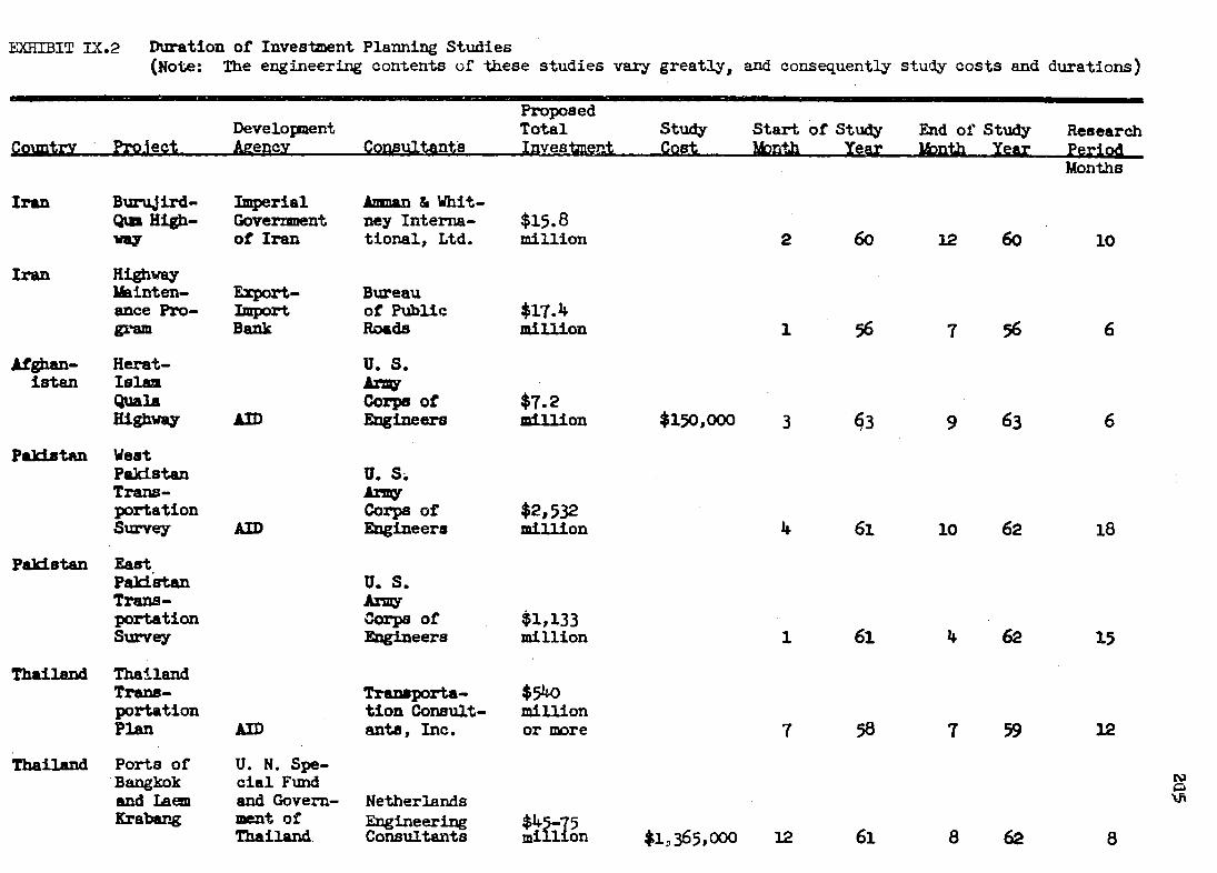
L=GI'hIT IX.2 Duration of Investment Planning Studies (Note: The engineering contents of these studies vary greatly, and consequently study costs and durations)
Proposed Development Total Study Start of Study End of Study Research
Country Proiect Azency Consultants Investent Cost Month Year Ionth Year Period Months
Iran Burujird- Imperial Amman & Whit-Qum High- Government ney Interna- $15.8 way of Iran tional, Ltd. million 2 60 12 60 10
Iran Highway Ibinten- Export- Bureau ance Pro- Import of Public $17.4 gram Bank Roads million 1 56 7 56 6
Afghan- Herat- U. S. istan Islam Arsw
Quala Highway AID
Corps of Engineers
$7.2 million $150,000 3 63 9 63 6
Pakistan West Pakistan U. S. Trans- Army portation Corps of $2,532 Survey AID Engineers million 4 61 10 62 18
Pakistan East Pakistan U. S. Trans- Aray portation Corps of $1,133 Survey Engineers million 1 61 4 62 15
Thailand Thailand Trans- Tranaporta- $540 portation Plan AID
tion Consult-ants, Inc.
million or more 7 58 7 59 12
Thailand Ports of U. N. Spe-Bangkok cial Fund and Laem and Govern- Netherlands KrabTlg ment of
Thailand. Engineering Consultants
$4 7 million
15 $1, 365,000 12 61 8 62 8
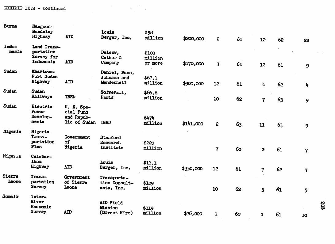
EXHIBIT IX.2 - continued
Bura Rangoon-IbndalayHighway
Ido- Land Transnesia portation
Survey for Indsaia
Sudan Mlahtom-Part SudanHighway
Sudan Sudan Railways
Sudan Electric Power Develop-ments
Nigeria Nigeria Trane-portation Plan
Nigeria Calabar-Ikcm Highway
Sierra Trans-Leone portation
Survey
SmalJa Inter-River
Econcmic Survey
AID
AID
AID
IBRD
U. N. Special Fund and Repub-lic of Sudan
Government of Nigeria
AID
Government of Sierra Leone
AID
LouisBerger, InC.
DeLeuw, Cather & CcMrpeny
Daniel, Mann, Johnson and1endenha11
Sofrerail, Paris
IBRD
Stanford Research Institute
Inuis Berger, Inc.
Transportation Consult-ants, Inc.
AID Field EUAsion (Direct Hire)
$58million
$100 million or mre
$67.1million
$86.8 million
$474 million
$220 million
$11. 1 million
$109 million
$119 million
$200,000
$170,000
$900,000
$141,000
$350,000
$76,000
2
3
12
10
2
7
12
IO
3
61
61
61
62
63
60
61
62
60
12
12
4
7
11
2
7
3
1
62 22
61 9
62 4
63 9
63 9
61 7
62 7
61 5
61 10

EXHIBIT IX.2 - continued
Somalc a
Libaria
Port of kzffdiBcio
Liberia Tr-portationSurvey
AID
AID
U. S. Army Corpa ofEngineers
BrownEngineers
$8million
$23 million or more i82,00
4
4
63
63
8
8
63
63
4
Tangan-yika
Honduras
Argentinn
Bolivia
Bolivia
Highway Reconnais-sance
Hor-uraa Ten-Year HighwayProgram
Argentina Trans-portation Plan
Three High-ways in Guabir Region
Yapaceani Highway Brd Bridge
AID
IDA and Republic ofHonduran
U. N. Special Fund and Republic of Argentina
AID
m AID
Tudor EngineeringCo.
Stanford ResearchInstitute
IBRD
Tippetts-Abbett-
WCarthy-Stratton
Tippetts-Abbett
cartby-Stratton
$135million
$900 million
$6 million
$3.1 million
$200,000
$1,045,0OO
$85,500
$171,000
8
3
3
7
7
62
62
60
62
62
10
1
2
4
62
63
62
63
63
2
10
23
10
9
Range of Observed Research Periods (Jbntha):Average Research Period (Months): 9.5
2 to 23
218
analyses can be accomplished faster if enough personnel are put on the job.
The highway reconnaissance study in Tanganyika was of that latter type and
was also, with only two months' duration, the fastest.
Looking at the other extreme, the four studies dealing with the biggest
investments, ranging from $0.5 billion to $2.5 billion, all required preparations
of a year or more. The Argentine Transportation Study was the most ambitious
effort in terms of methodology, had the highest cost ($1 million) and, with 23
months' research period, took the longest time to prepare. There is also a
rough correspondence between study length and size of proposed investment
of the other three large-scale efforts: the West Pakistan Transportation Plan
(with contemplated investment of $2.5 billion), took 18 months; the East Pakistan
one (with contemplated investment of $1.1 billion) took 15 months, and the
Thailand one (with contemplated investment of $540 million or more) took 12
months.
But looking at the remaining array of studies by size of investment,
it is impossible to detect any logical pattern for the remaining 18 reports.
One can only conclude that the four most ambitious pre-investment reports
took rather long to prepare, but that the rest display a great diversity of
research periods. The "average" time taken is 9 1/2 i-nonths, but because
of the great dispersion of the values around the mean not athis is very
meaningful figure. However, 17 out of 23 studies fall into the range of 4
to 10 months, and this is a useful finding.
219
rime Intervals in AID Investment Process
Exhibits IX.3 and IX.4 give the life histories of 18 AID projects,
from the completion of the last investment study relating to each particular
one, through loan authorization, to first money disbursement and, in some
instances, to final money disbursement. It was unexpectedly difficult to
get this information- -much of it had to be obtained by personal interviews,
or by tracing project files- -resulting in the present small sample. A few
methodological problems should be noted:
1. The projects could not be selected in any random or systematic
manner, but the attempt was made to get some from each of AID's geo
graphic regions and to emphasize transportation projects.
2. The completion of project appraisal is often hard to pinpoint.
There can be entire chains of studies, with the second re-evaluating the
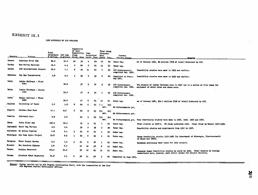
EXHIBIT 1X.3
LmFnHISlS OF AID PROJECTS
Completionof last First Ibney
Total Feasibility loan Disburse-Investment AID loan Study Authorized ment Current
o~ntry ec% ......ton -' Lnth Year a ' e Ao re Q $8 , Greece Acheloos River Dam 82.0 31.0 10 59 Ii 60 10 60 Under way. As of Janur l96, * million (% of tota) disbused by AID. Turkey Ms-Tatvan Railroad 18.0 4.3 2 60 6 60 12 63 Under way. Israel LD International Airport 19.0 1.1 6 59 11 60 4 63 iD disburements Feasibility studies were made in 1959 and earlier.
completed Jan. 1964.Padstan sd can Transmission 2.8 2.0 591 3 59 6 60 Completed in Febru- Feasibility studies were made in 1959 and earlier.
ary 1961.Inda Idia Railwys. First Inn3.0i 5In 2an AID dlbursement Teo studies of Indian Ralwa done in 1957 led to a series of five loans for
completed Jan. 196. equjiment of which three are shown here. India indian Railwaya - Second
loan 35.0 57 5A9 1 59 AID disbursement copleted Jan. 1961.
India" Indian Ulailrays - Third 50.0 57 6 60 1oIQn 61 Under way. As or ji.umam196., $1,2.7 mion (85% of total) disbursed by AID.
.Tumisia University or unis 3.2 1.8 6 60 6 63 (1 65) eat. No disbursements yet.Nigri.a alabar-I- Road fl.1 8.6 6 62 a 63 (1 64)
est. No disbursements yet.5s tla ( isim o Port 3.9 3.6 60o 63 (10 -61)eat. No disbursements yet. Four feasibility studies were mde in .1954, 1959, 1960 and 1960.0.a Volta River Dom 196.0 20.0 59 5 61 1 63 Under way. Firat studied in 1920,s. UX study published 1956. Final study bytalser 1957-1959. uatemala Kenf Bag Factory 0.9 0.4 5 2 59 9 59 Under way. Feasibility studies and experiments from 1952 to 1958.
Guatmala El iblino Higheay 4.8 2.1 3 60 8 60 5 62 Under way. Nicaragua Rio Tuma Fydro Project 20.8 2.5 1 60 6 60 5 61 Under way. Three feasibility studies 1955-1960 (by Government of Nicaragua, Ilectroconsult
of Milan "d mm).Paraguay Water Supply System 9.5 1.0 3 55 6 58 1 59 Under way. Eisbank previously made loans for this project. Ecuddor Pan imerican Highway 5.4 1'7 57 12 58 8 59 Under way. Taiwan Tachlen Reservoir 109.7 10.0 58 12 * 60 10 61 Under way. Japanese began feasibility studies as early as 1935. Other reports by foreign
consultants were, however, more direct causes for project decision. Taian Alumnum Plant ]epension 8&.8 1.3 6 1158 58 3 60 Complsted in June 1963.
Source: SuTey carried cut by AID Program Coordination Staff, with the cooperation of the fourAD Regional Capital Development Ofices.
221
first, and the third building up or, the second. For the present survey, the
date of completion of the last known project study was used, since interest
here is centered on the length of the decision-making and action processes
and these are presumably set into motion by the last study document.
3. Conversely, one feasibility study can start off a series of projects
extending over several years. This is so in the case of the Indian railway
equipment loans, where the report was completed in 1957 and the money dis
bursements extend from 1958 through to the present time. Here long time
intervals are to be expected, with the borrower drawing on funds as railway
rolling stock, for example, gradually wears out and has to be replaced.
So-called stage construction, again based on a single project appraisal,
would have similar effects.
4. In the course of the survey it also became apparent that due to
frequent organizational changes in the past and many transfers of personnel,
among other causes, the records of the Agency often did not reach back very
far. Numerous projects had no records of any feasibility study as such, while
others had records of more than one.study." Again, a number of studies were not
done specifically for AID. Complete, well-documented life histories were
therefore rare.
The results drawn from this admitiedly small and unrepresentative sample
are shown in Exhibit IX.4. There is a great variation in the time con
sumed by AID in moving from one stage in the investment cycle to the next.

EXHIBIT IX.4
TAL9 I AID N PR
From Com- Total Time Time Consumption frompletion Interval Feasibility Study toof Last From "an from Last Project Completion,Feasibil- Authori- Feasibili- where Applicable.ity Study zation ty Study (In brackets: For proto Loan to FirstTotal to FirstAuthori- Money Dis- Money Dis-jects still under way,
Investment Time already ConsumedAID loan zation bursemente2Mliin bursementsMillio Months as of June 30, 1964).Months nthsGreece Acheloos River Dam 82.0 31.0 66 12 (56+)Turkey Mus-Tatvan Railroad 18.0 4.3 4 42 46 (52+)Israel LOD International Airport 19.0 1.1 17 29 46 55Pakistan Sul Gas Transmission 2.8 2.0 2 15 17 25 India Indian Railways - FirstLoan
30.0 II 9 20 79 India Indian Railways - Second a/Loan
35.0 15 4 19 79 India Indian Railways - Thirdloan Tunisia University of Tunis
50.0 36 16 52 (V4)3.2 1.8 369 1/1- 51/55 No disbursements yet.Nigeria Calabar-lkom Road Ii.i 8.6 14 15 29 No disbursements yet.Somalia Chisimrio Port 3.9 3.6 35 17 52 No disbursements yet.
Ghana Volta River Dam 196.o 20.0Guatemala 20Kenof Bag Factory
23 43 (6c)0.9 0.4 53 7 15 (72+-)Guatemala El Molino Highway 2.14.8 5 21 2 (51+)Nicaragua Rio Tlur Hydro Project 20.P 2.5 5. 11 Paraguay Water
16 531)Supply System 9.5 1.0 39" , frf-)

E RHIBIT EA.4 - continued
Ectador Pa Amrican Highw 5.4 L7 is :6 (84+)
Taiwan Tamhien Reservoir 109.7 40.0 0 10 40 (72+)
Taiwan Aluminum Plant Expansion P4.8 1.3 5 16 .21 60
Observed Range (Months) 2 to 39 6 to 42 12 to 55 25 to (111+)
Average (Months) 16.6 15.1 31.7
Va Mid-year assumed for completion of last feasibility study, when exact m=th not known.
A/ Estimates of loan officers.
Source: Derived from Exhibit IX.3.
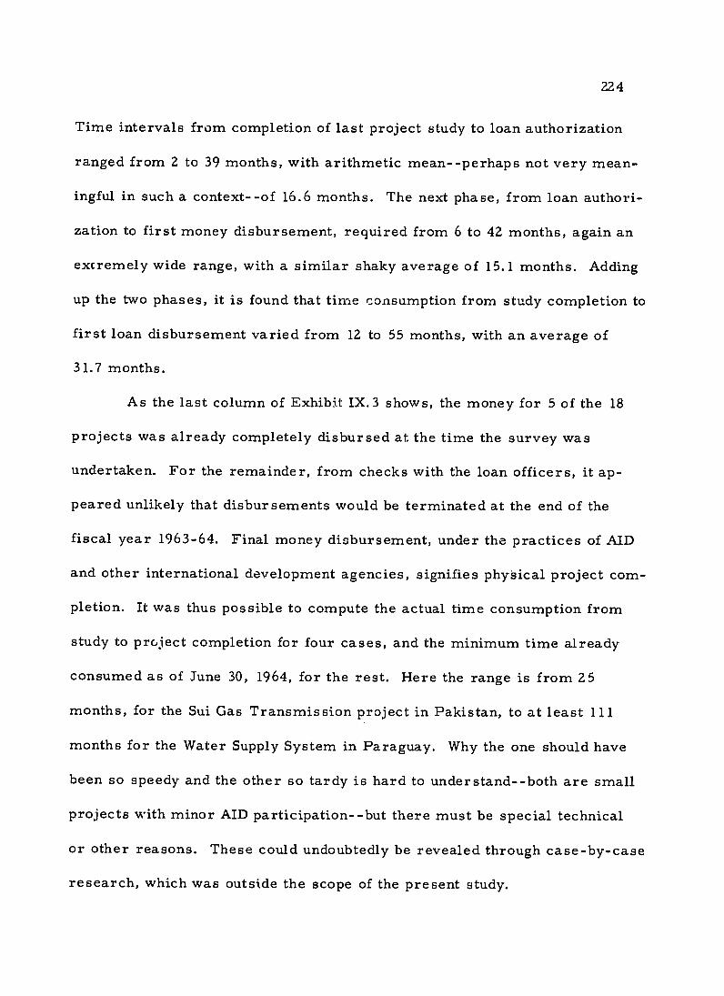
224
Time intervals from completion of last project study to loan authorization
ranged from 2 to 39 months, with arithmetic mean--perhaps not very mean
ingful in such a context--of 16.6 months. The next phase, from loan authori
zation to first money disbursement, required from 6 to 42 months, again an
excremely wide range, with a similar shaky average of 15.1 months. Adding
up the two phases, it is found that time consumption from study completion to
first loan disbursement varied from 12 to 55 months, with an average of
31.7 months.
As the last column of Exhibit IX.3 shows, the money for 5 of the 18
projects was already completely disbursed at the time the survey was
undertaken. For the remainder, from checks with the loan officers, it ap
peared unlikely that disbursements would be terminated at the end of the
fiscal year 1963-64. Final money disbursement, under the practices of AID
and other international development agencies, signifies physical project com
pletion. It was thus possible to compute the actual time consumption from
study to prcject completion for four cases, and the minimum time already
consumed as of June 30, 1964, for the rest. Here the range is from 25
months, for the Sui Gas Transmission project in Pakistan, to at least 111
months for the Water Supply System in Paraguay. Why the one should have
been so speedy and the other so tardy is hard to understand- -both are small
projects with minor AID participation- -but there must be special technical
or other reasons. These could undoubtedly be revealed through case-by-case
research, which was outside the scope of the present study.

225
Can some generalizations be made on these 18 project life histories?
If the three slowest and the three fastest projects are left out in each case,
the following ranges result for the remaining twelve:
1. From completion of study to loan authorization: 5 to 35 months.
2. From loan authorization to first money disbursement: 7 to 20
months.
3. Combined, from study completion to first money disbursement:
17 to 46 months.
If the Pakistani Gas Transmission project, as an exceptionally speedy
one, is left out, one observes that the remaining 17 projects took at least 51
months, or well over four years, to move from investment analysis to physical
project completion. If we add to that the 4 to 10 months typically required to
carry out the investment analyses themselves, we find that 55 to 61 months of
minimum time consumption, from start of feasibility study to project com
pletion, can be put down as a tentative first result. It is readily appreciated
that the length of the "pr6ject pipeline," from research through action com
pletion--at least 4 1/2 to 5 years--has great implications for economic arid
financial planning.
Time Intervals Between First and Final AID Disbursements
To get further evidence on project life histories, an additional
survey on loan disbursement patterns was carried out in coordination
with Agency personnel. The research technique was to select
projects shown as 100 percent completed in recent AID

226
progress reports and then to work back over the years to the time of the
very first disbursement. By using quarterly and bi-annual AID progress
reports in preference to annual ones, whenever possible, it was possible to
date the first and last disbursements fairly accurately. Much better docu
mentation was available on the disbursement phases and a sample of 31
projects was obtained (Exhibit IX.5).
Money disbursement is a good indicator for physical project progress
because the last payments are usually held up until there has been a check
that the contractor has lived up to his obligations and the factory, electric
power plant, highway or whatever it may be really conforms to specifications.
It often happens in the case of AID projects,( and IBRD has had similar experi
ences) that the great bulk of expenditures is met fairly early during project
construction and that then there is a "trickle effect," which may go on for
several years, with rather small sums of money being disbursed as the
contractors finish up minor details. The projects with special remarks in Ex
hibitIX.5 are of this type; although 80 or 90 percent of the total costs have
already been met, they may yet go on for quite some time.
Looking at the results as a whole, the great variations in disbursement
patterns are remarkable. The range from loan agreement to first disburse
ment is from 1 to 41 months, with a questionable average of 10.8 months.
The next phase, from the first to the last money disbursement, takes from
5 to 55 months or more; the average for completed projects is 19.9 months,

Er-'TBIT iX.5 RadUa S mple of AID Loans Showing Time Span Between Loan Agreements and First and Final Disbursements
cndI& and N'uber
Nigeria DI 75
Nigeria DIF 161
Ethiopia. DIF 88
LibyaDLF 24
Tumisia DIF 136
ProLect
Nigeria Port AuthorityWarehouseCowatruct0on
Nigeria Railway Corpora. tion TrackRelaying
Sviluppo Apicolo Industriale del ]rit2re-Cotton Tex-tile n.f
Govt. ofLibya Else-tric PowerPlant
Societe Nationaledes Cheuins
Ra ti ay Rala
Date of Xoan Agree-ment and Amount ( l/
12-Wr059
8-31-61$3.0
8-6-59*0.5
62.59*5.0
$ 2 .8 92.
Date of First Dis-bursent
7-60
9-61
3-60
3-60
9 -61b-1(12-63)
Date of Last Dis-buraeent
V]
12-6o
-62
9-61
(12-63)
Time Interval
froM Loan Agreementto First Disburse-mnt (Months)
7
1
7
9
28
Interval fr= First Disburse-ment toLast Dis-bursement
l (IMnths)
5
U-,
18
(4i5+)
(2.7+)
Time Interval frcx Loan Agreementto Last Disbursemoet (Ibnths) Remarks
12
12
25
8 millio
(51rs) d as of
2. zdi..UM ur s ed as o f
(55+) date Shown
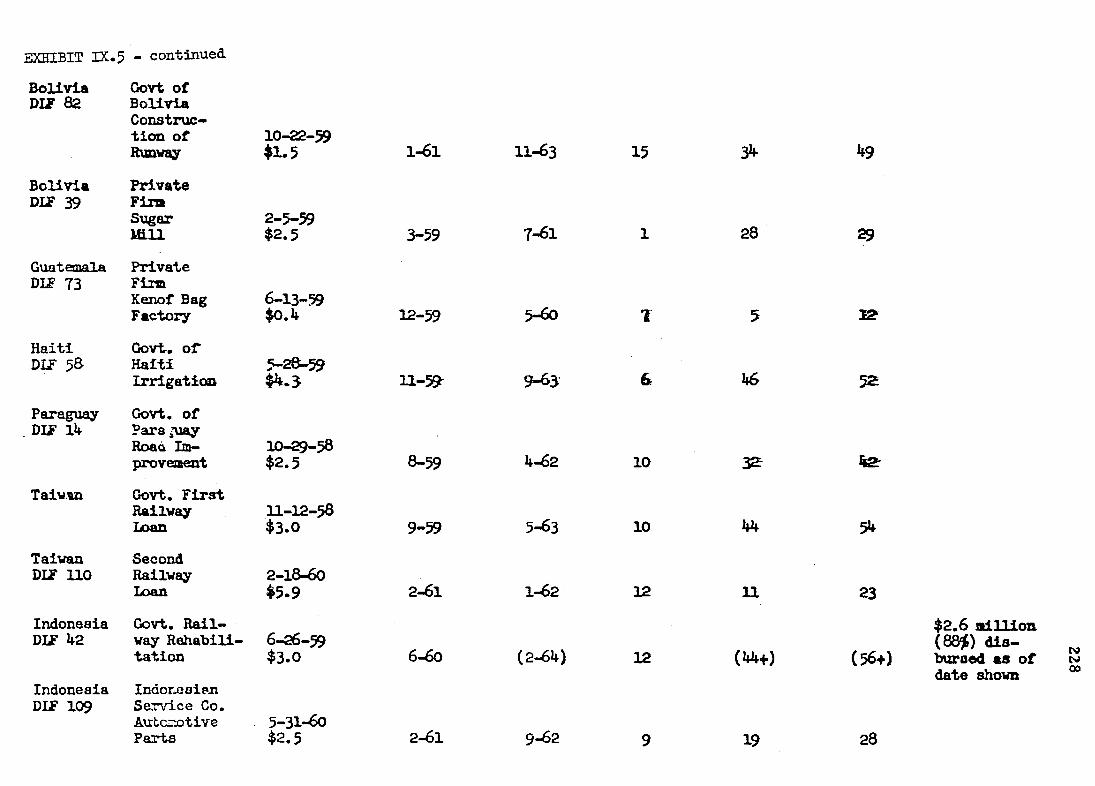
EXHIBIT IX.5 - continued
Bolivia Govt of DIF 82 Bolivia
Construction of 10-22-59 RMWV $1.5 1-61 11-63 15 34 49
Bolivia Private DL 39 Firm
Sugar 2-5-59 $2.5 3-59 7-61 1 28 29
Guatemala Private DIF 73 Firm
Kenof Bag Factory
6-13-59 $0.4 12-59 5-60 1 5 32
Haiti Govt-. of DLF 58 Haiti 5-28
Irrigation $4.3 U-59 9-63 & 46 5Z
Paraguay Govt. of DIF 14 Pars ua"y
RoadL Im- 10-29-58 provement $2.5 8-59 4-62 10 -i ra
Taiwin Govt. First Railway 11-12-58 Loan $3.0 9-59 5-63 10 44 54
Taiwan Second DIF iiO Railway 2-18-60
Loan $5.9 2-61 1-62 12 11 23
Indonesia DIE 42
Govt. Rail-way Rehabili- 6-26-59
$2.6 million(88.) i- n
ttion $3.0 6-60 (2-64) 12 (14+) (56+) burned as of date shown
, o
Indonesia Indoresid
DIF 109 Sea-vice Co. Autrotive 5-31-60 Parts $2.5 2-61 9-62 9 19 28
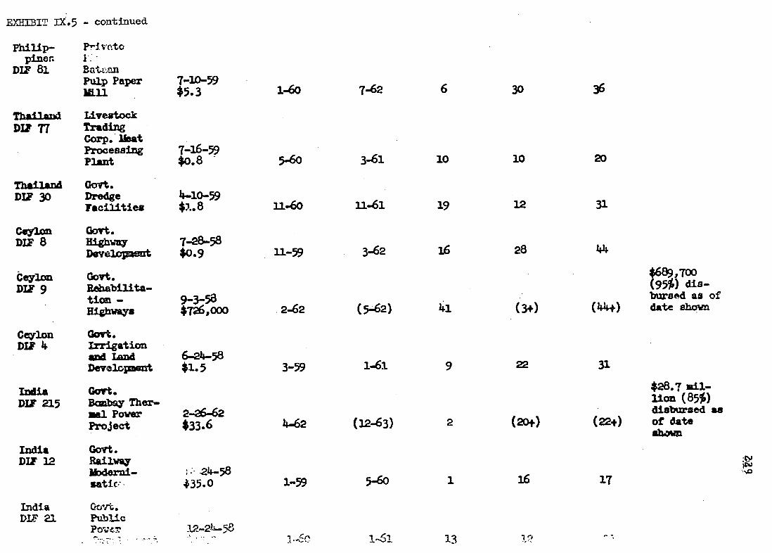
EXHIBIT IX.5
Philip-pinery
DI 81
Thai d DLF 77
Thailand DII 30
Ceylon DII 8
Ceylan DIF 9
Ceylon DIF 4
India DL? 215
India DIF 12
India DIF 21
- continued
P'I nte 1. * BatLz-an Pulp Paperm
Livestock Trading Corp. That Processing plant
Govt. Dredge Facilities
Govt. Highway Develoyimt
Govt. Rehabilita-tim -Higways
Govt. irrigation an Land Development
Gort. Bdb ay Ther-mal Power Project
Govt. Railway Moderni-satic-
Got. PublicP ov• -. 'p . . .. .
7-10-59$5.3 1-60
7-16-59 $0.8 5-60
4-10-59 V. 8 11-60
7-28-58 $0.9 11-59
9-3-58 $726,000 .2-62
6--24-58 $1.5 3-59
2-26-62 $33.6 4-62
;- 24-58435.0 1-59
-'22l .5 8 . .w.,c,,
7-62
3-61
11-61
3-62
(5-62)
1-61
(12-63)
5-6o
-r1
6
10
19
16
41
9
2
1
30
10
12
28
(3+)
22
(20+)
1.6
.."'
36
20
31
44
(44+)
31
(22-)
17
68700 ) dis
bureed a of date ehoim
$28.7 llion (85%) disbursed as of date

EXHIBIT IX.5 - continued
India Govt. DIF 131 Road 6-30-60
Transport $13.1 3-61 7-62 9 16 25
Iran Plan DII' 97 Organization
HighwayConstrution
10-7-59 $25.0 6-60 6-61 8 12 20
0 A 10-7-59
$26.2 6-61 5-63 20 23 43
a B 10-7-59
$12.0 8-61 u-62 22 15 37
Pakistan Sui Gas Co. .DIF 74 Expansion
of Gam Treating 1-16-60 Plant $2.0 6-60 2-61 5 8 13
Pakistan Govt. DLF 186 Third 6-14-61
Railways $6,500,000 12-61 7-63 6 19 25
Pakistan Govt. DIF 86 jet 1l-3-59
Rimm7 43.0 4-60 1-62 5 21 26
Pakistan Govt. #9.0 million DIF 20 Railway
Rehabili- 2-18-59 burse) aisofbrsed as ef tation $9.1 8-59 (2-64) 6 (54) (6+) date n 0
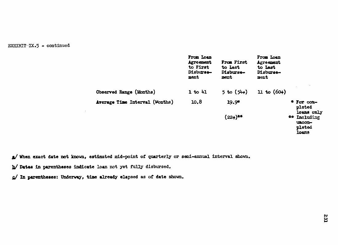
EXHIBIT IX.5 - continued
Frcm Loan Agreement to First Disburse-ment
Fro First to Last Disburse-nent
From IAmn Agreeent to Last Disburemert
Observed Range (lMths) 1 to 41 5 to (5+) 31to (600)
Average Time Interval (Months) 10.8 19.9*
(22+)**
* For ccmpleted loans Caly incl.tng
pleted loans
/ When exact date not known, estimated mid-point of quarterly or semi-annual interval shown.
]j/ Dates in parentheses indicate loan not yet fully disbursed.
g/ In parentheses: Underwa., time already elapsed as of date shown.

232
but when those are included which were not finished when the survey was
taken, this average rises to at least 22 months. Combined, the 31 projects
took between 11 months to 60 months and more from loan agreement to last
disbursement.
Looking at individual cases in Exhibit IX.5, one may venture to say that
some of the speedy projects are also very straightforward, small ones: Nigeria
Warehouse Construction ($0.7 million, 12 months from agreement to completion);
Nigeria Railway Track Relaying ($3.0 million, 12 months); Guatemala Bag Factory
($0.4 million, 11 months); Pakistan Gas Treating Plant ($2.0 million, 13 months).
Conversely, as one would expect, some of the large, complex projects take
longer to complete: three Iran Highway Construction Projects (20 months,
43 months, 37 months); rehabilitation and re-equipment of rail vays in Tunisia
(55 months and up), Taiwan (54 and 23 months), Indonesia (56 months and up),
India (38 months and up), Pakistan (25 months, 60 months and up).
And yet, there are some odd cases which are hard to explain on the
basis of the facts on hand. Bolivia Runway Construction, for which AID lent
$1.5 million and which one would think to be a rather simple technical undertaking,
took 49 months from loan agreement to completion. The $4.3 million Haiti
Irrigation Project consumed 52 months in all; but the "trickle effect" applies,
in this case, since $4.0 million, or 94 percent of the total, was already dis
bursed by June 30, 1962, or 37 months after the loan agreement. Seemingly
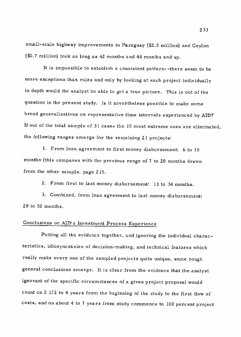
233
small-scale highway improvements in Paraguay ($2.5 million) and Ceylon
($0.7 million) took as long as 42 months and 44 months and up.
It is impossible to establish a consistent pattern--there seem to be
more exceptions than rules and only by looking at each project individually
in depth would the analyst be able to get a true picture. This is out of the
question in the present study. Is it nevertheless possible to make some
broad generalizations on representative time intervals experienced by AID?
If out of the total sample of 31 cases the 10 most extreme ones are eliminated,
the following ranges emerge for the remaining 2 1 projects:
1. From loan agreement to first money disbursement: 6 to 15
months (this compares with the previous range of 7 to 20 months drawn
from the other sample, page 2 15.
2. From first to last money disbursement: 11 to 34 months.
3. Combined, from loan agreement to last money disbursement:
20 to 52 months.
Conclusions on AID's Investment Process Experience
Putting all the evidence together, and ignoring the individual charac
teristics, idiosyncrasies of decision-making, and technical features which
really make every one of the sampled projects quite unique, some rough
general conclusions emerge. It is clear from the evidence that the analyst
ignorant of the specific circumstances of a given project proposal would
count on 2 1/2 to 4 years from the beginning of the study to the first flow of
costs, and on about 4 to 7 years from study commence to 100 percent project

234
completion. These lead times would have to-be increased for exceptionally
large, technically complex projects which do not seem to fit well in'to usual
AID procedures and plans, or for projects located at remote sites in
politically unstable countries of small abso: ptive capacity and with supply
and labor problems. Conversely, these potential time lags could be reduced
wherever the opposite conditions prevail.
239
GENERAL CONCLUSIONS
The pilot studies demonstrate quite vividly the very long lead times-
five to seven or more years from start to finish--with which one has to reckon
in investment planning in developing countries. This is something which policy
makers, scholars and field analysts have perhaps not fully appreciated previously.
A few general conclusions can be offered:
1. The frequent failures of national development plans to live up to
expectations may partly be due to the extremely long gestation periods be
tween idea, plan, decision, action and the harvesting of benefits.
2. Comparing the average time taken by the various stages in the
investment process, it seems that the field studies have perhaps been un
necessarily rushed relative to the deliberation and decision-making stages.
A study period in the field of four or five months to appraise a $50 or $100
million investment appears far too short.
3. Regardless of whether or not there is an imbalance between the
efforts going into investment studies, on the one hand, and into investment
decisions and actions, on the other, structural changes in the investment
process for economic development must be considered. For example, the
sequence might run as follows:
a. Sectoral studies which analyze the entire range of investment
alternatives within a sector and indicate broadly the optimum allocation of
resources there.
240
As a practical matter, it is not possible to compare all
possible investment alternatives in arriving at a decision concerning a
single project. But external effects of various sorts and inter-dependencies
among projects and over time are very important in the developing countries.
Project studies, by their very nature, are too narrowly framed to consider
such matters.
b. Pre-investment reconnaissance, with preliminary findings being
submitted to the international agency and the government of the less developed
nation after three or four months.
This would be a small-scale expert appraisal of a broad range
of alternatives. Its purpose would be to determine whether the productive
potential, market potential, and investment plans for the economy concerned
warrant an improvement of any kind, and, if so, what, where and when. Only
the broadest questions about the project alternatives under study would be
answered at this stage.
c. If the first crude findings are encouraging, the decision-making
machinery in both the developing country and the development agency could start
to move, and the field analysts could be given the green light to embark upon
the more detailed and costly phases of their studies. But if investment pros
pects are not good, the planners can immediately turn away to more fruitful
inve stigations.
d. As more precise results become available from the field perhaps
five to eight months later, they could be used immediately for final decision

241
making purposes. This would have the advantage that the research information
before the executives at that crucial moment would be up-to-date.
e. Assuming that there is a favorable decision on the basis of
fresh evidence, the detailed analytical work might very naturally merge right
into the final engineering, location, design and contract-letting phases.
What is visualized here are, in effect, two parallel chains--one of
planning and analysis, the other of decision-making, budgeting and the like-
rather than one consecutive chain of discrete investment phases as seems to be
the general practice now. In terms of Exhibit IX.1, the suggestion is to let
Stage D (the investment analyses) continue at the same time as Stages E and F
(decision-making up to action agreement) progress. In the end, this expanded
Stage D might be connected up with Stage G, the investment action phase, which
has a strong field survey content of its own (see Exhibit IX.6). The engineering
emphasis should become greater and greater as it approaches Stage G.
It is possible that such a double chain of investment stages would re
sult in shorter duration for the process as a whole, superior functional conti
nuity and the provision of fresher information to the decision makers. In fact,
such schemes already exist-- continuous long-range planning practices in some
parts of the world and by some international agencies is basically of this nature.
It would be worthwhile to investigate how the discrete phases of project invest
ment planning could best be fitted into the continuous sector and economy-wide
development plans of the future. Critical path diagramming and related
analytical techniques could be used to advantage to tackle these problems.
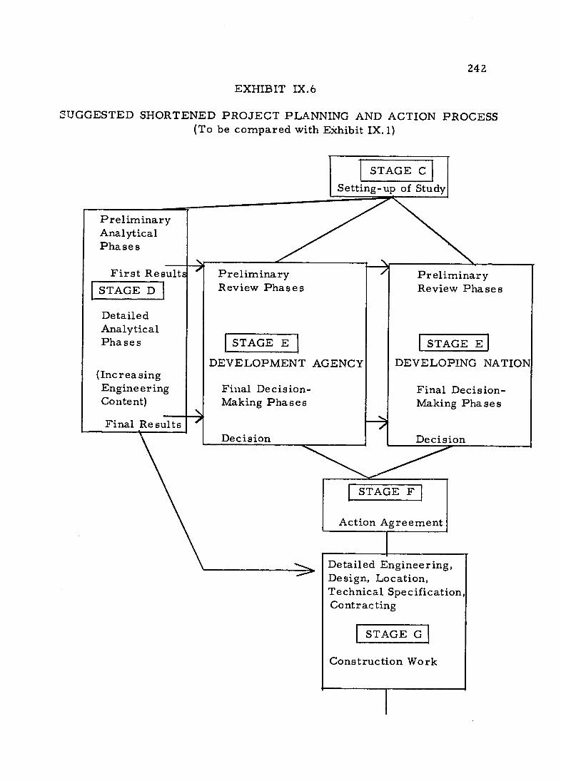
242
EXHIBIT IX.6
OUGGESTED SHORTENED PROJECT PLANNING AND ACTION PROCESS (To be compared with Exhibit IX. 1)
Setting-up of Study
Preliminary
Analytical Phases
First Result Preliminary Preliminary
STAGE D Review Phases Review Phases
Detailed Analytical
Phases iSTAGE STAGE E
DEVELOPMENT AGENCY DEVELOPING NATION (Increasing Engineering Final Decision- Final Decision-Content) Making Phases Making Phases
Final Results Decision Decision
Action Agreement
Detailed Engineering, Design, Location, Technical Specification, Contracting
Construction Work