pdfs.semanticscholar.org · 2017-05-15 · AFRL-RQ-WP-TR-2015-0151 . HIFiRE-5 BOUNDARY LAYER...
68
AFRL-RQ-WP-TR-2015-0151 HIFiRE-5 BOUNDARY LAYER TRANSITION AND HIFiRE-1 SHOCK BOUNDARY LAYER INTERACTION Roger L. Kimmel, Matthew P. Borg, and Joseph S. Jewell Hypersonic Sciences Branch High Speed Systems Division James H. Miller Vehicle Technology Branch High Speed Systems Division Dinesh Prabhu NASA Ames Research Center OCTOBER 2015 Interim Report Approved for public release; distribution unlimited. See additional restrictions described on inside pages STINFO COPY AIR FORCE RESEARCH LABORATORY AEROSPACE SYSTEMS DIRECTORATE WRIGHT-PATTERSON AIR FORCE BASE, OH 45433-7541 AIR FORCE MATERIEL COMMAND UNITED STATES AIR FORCE
Transcript of pdfs.semanticscholar.org · 2017-05-15 · AFRL-RQ-WP-TR-2015-0151 . HIFiRE-5 BOUNDARY LAYER...
AFRL-RQ-WP-TR-2015-0151
HIFiRE-5 BOUNDARY LAYER TRANSITION AND HIFiRE-1 SHOCK BOUNDARY LAYER INTERACTION Roger L. Kimmel, Matthew P. Borg, and Joseph S. Jewell Hypersonic Sciences Branch High Speed Systems Division James H. Miller Vehicle Technology Branch High Speed Systems Division Dinesh Prabhu NASA Ames Research Center OCTOBER 2015 Interim Report
Approved for public release; distribution unlimited.
See additional restrictions described on inside pages
STINFO COPY
AIR FORCE RESEARCH LABORATORY AEROSPACE SYSTEMS DIRECTORATE
WRIGHT-PATTERSON AIR FORCE BASE, OH 45433-7541 AIR FORCE MATERIEL COMMAND
UNITED STATES AIR FORCE

NOTICE AND SIGNATURE PAGE
Using Government drawings, specifications, or other data included in this document for any purpose other than Government procurement does not in any way obligate the U.S. Government. The fact that the Government formulated or supplied the drawings, specifications, or other data does not license the holder or any other person or corporation; or convey any rights or permission to manufacture, use, or sell any patented invention that may relate to them. This report was cleared for public release by the USAF 88th Air Base Wing (88 ABW) Public Affairs Office (PAO) and is available to the general public, including foreign nationals. Copies may be obtained from the Defense Technical Information Center (DTIC) (http://www.dtic.mil). AFRL-RQ-WP-TR-2015-0151 HAS BEEN REVIEWED AND IS APPROVED FOR PUBLICATION IN ACCORDANCE WITH ASSIGNED DISTRIBUTION STATEMENT. *//Signature// //Signature// ROGER L. KIMMEL MICHAEL S. BROWN, Chief Project Manager Hypersonic Sciences Branch Hypersonic Sciences Branch High Speed Systems Division High Speed Systems Division Aerospace Systems Directorate //Signature// THOMAS A. JACKSON Deputy for Science High Speed Systems Division Aerospace Systems Directorate This report is published in the interest of scientific and technical information exchange, and its publication does not constitute the Government’s approval or disapproval of its ideas or findings. *Disseminated copies will show “//Signature//” stamped or typed above the signature blocks.
REPORT DOCUMENTATION PAGE Form Approved OMB No. 0704-0188
The public reporting burden for this collection of information is estimated to average 1 hour per response, including the time for reviewing instructions, searching existing data sources, searching existing data sources, gathering and maintaining the data needed, and completing and reviewing the collection of information. Send comments regarding this burden estimate or any other aspect of this collection of information, including suggestions for reducing this burden, to Department of Defense, Washington Headquarters Services, Directorate for Information Operations and Reports (0704-0188), 1215 Jefferson Davis Highway, Suite 1204, Arlington, VA 22202-4302. Respondents should be aware that notwithstanding any other provision of law, no person shall be subject to any penalty for failing to comply with a collection of information if it does not display a currently valid OMB control number. PLEASE DO NOT RETURN YOUR FORM TO THE ABOVE ADDRESS.
1. REPORT DATE (DD-MM-YY) 2. REPORT TYPE 3. DATES COVERED (From - To)October 2015 Interim 31 October 2014 – 15 October 2015
4. TITLE AND SUBTITLEHIFiRE-5 BOUNDARY LAYER TRANSITION AND HIFiRE-1 SHOCK BOUNDARY LAYER INTERACTION
5a. CONTRACT NUMBER In-house
5b. GRANT NUMBER
5c. PROGRAM ELEMENT NUMBER 61102F
6. AUTHOR(S)
Roger L. Kimmel, Matthew P. Borg, and Joseph S. Jewell (AFRL/RQHF) James H. Miller (AFRL/RQHV) Dinesh Prabhu (NASA Ames Research Center)
5d. PROJECT NUMBER 3002
5e. TASK NUMBER N/A
5f. WORK UNIT NUMBER
Q1FN 7. PERFORMING ORGANIZATION NAME(S) AND ADDRESS(ES) 8. PERFORMING ORGANIZATIONHypersonic Sciences Branch (AFRL/RQHF) Vehicle Technology Branch (AFRL/RQHV) High Speed Systems Division Air Force Research Laboratory, Aerospace Systems Directorate Wright-Patterson Air Force Base, OH 45433-7541 Air Force Materiel Command, United States Air Force
NASA Ames Research Center Moffett Field, CA 94035
REPORT NUMBER
AFRL-RQ-WP-TR-2015-0151
9. SPONSORING/MONITORING AGENCY NAME(S) AND ADDRESS(ES) 10. SPONSORING/MONITORINGAir Force Research Laboratory Aerospace Systems Directorate Wright-Patterson Air Force Base, OH 45433-7541 Air Force Materiel Command United States Air Force
AGENCY ACRONYM(S)AFRL/RQHF
11. SPONSORING/MONITORINGAGENCY REPORT NUMBER(S)
AFRL-RQ-WP-TR-2015-0151 12. DISTRIBUTION/AVAILABILITY STATEMENT
Approved for public release; distribution unlimited.13. SUPPLEMENTARY NOTES
PA Case Number: 88ABW-2015-4531; Clearance Date: 22 Sep 2015.The U.S. Government is joint author of the work and has the right to use, modify, reproduce, release, perform, display, ordisclose the work.This is a work of the U.S. Government and is not subject to copyright protection in the United States.
14. ABSTRACTSeveral advances were made under this task during FY15, the first year of this effort. A portion of the task effort focusedon HIFiRE-5. For this work, new capabilities in ground test and in flight data analysis were developed. Also, as anecessary precursor to wind tunnel tests on boundary layer transition on the leeside of a cone at angle of attack, extensivecomputations were undertaken to understand the zero angle of attack instability behavior. Although not directly relatedto the topic of boundary layer transition, final analysis of the HIFiRE-1 shock boundary layer interaction experiment wascompleted.
15. SUBJECT TERMSboundary layer transition, hypersonic, flight test
16. SECURITY CLASSIFICATION OF: 17. LIMITATIONOF ABSTRACT:
SAR
18. NUMBEROF PAGES
68
19a. NAME OF RESPONSIBLE PERSON (Monitor) a. REPORT Unclassified
b. ABSTRACTUnclassified
c. THIS PAGEUnclassified
Roger L. Kimmel 19b. TELEPHONE NUMBER (Include Area Code)
N/A Standard Form 298 (Rev. 8-98) Prescribed by ANSI Std. Z39-18

i Approved for public release; distribution unlimited.
TABLE OF CONTENTS Section Page
LIST OF FIGURES ........................................................................................................................ ii LIST OF TABLES ......................................................................................................................... iv Acknowledgments........................................................................................................................... v 1. Summary ................................................................................................................................. 12. Introduction ............................................................................................................................. 33. Infrared and Pressure Measurements of Crossflow Instability ............................................... 7
3.1. Background and Experimental Overview ........................................................................ 7 3.2. Tunnel Freestream Characterization .............................................................................. 10 3.3. Quiet Flow ...................................................................................................................... 10
3.3.1. Stationary Crossflow Instability ............................................................................. 10 3.4. Traveling Crossflow Instability ...................................................................................... 16 3.5. Noisy Flow ..................................................................................................................... 20
3.5.1. IR Images ................................................................................................................ 20 3.5.2. Pressure Sensors...................................................................................................... 21
3.6. Summary and Conclusions ............................................................................................. 22 4. Correlation of HIFiRE-5 Flight Data with Computed Pressure and Heat Transfer .............. 23
4.1. Background .................................................................................................................... 23 4.2. Computations ................................................................................................................. 24 4.3. Pressure Distribution RMS Analysis and Comparison With CFD ................................ 28 4.4. Heat Transfer Distribution Analysis and Comparison with CFD ................................... 31 4.5. Axisymmetric Shell Heat Conduction Computations ..................................................... 32 4.6. Conclusions .................................................................................................................... 35
5. Boundary Layer Stability Analysis for Stetson’s Mach 6 Blunt Cone Experiments ............ 365.1. Background .................................................................................................................... 36 5.2. Computational Methods ................................................................................................. 36 5.3. Stability Computations ................................................................................................... 40
6. HIFiRE-1 Turbulent Shock Boundary Layer Interaction – Flight Data and Computations . 436.1. Background .................................................................................................................... 43 6.2. Instrumentation............................................................................................................... 45 6.3. Computations ................................................................................................................. 46 6.4. Pressure .......................................................................................................................... 49 6.5. Heat Transfer .................................................................................................................. 52 6.6. Conclusions and Future Work ........................................................................................ 53
7. References ............................................................................................................................. 54List of Acronyms, Abbreviations, Symbols .................................................................................. 59
ii Approved for public release; distribution unlimited.
LIST OF FIGURES Figure Page
Figure 1 Rollup of Boundary-layer into Streamwise Vortex on 2:1 Sharp Elliptic Cone, Similar to HIFiRE-5 (from Ref. ) .................................................................................4
Figure 2 Transition on the HIFiRE-5 Configuration in the Purdue Quiet Flow Ludwieg Tube at AoA=0 (left) and the Windward Surface at AoA=4 deg (right) (from Ref 10) ...........5
Figure 3 Filtered Rayleigh Scattering Image of Centerline Bulge of 2:1 Elliptic Cone13 ..............6 Figure 4 Photograph of Model ........................................................................................................8 Figure 5 Schematic of Pressure Sensor Locations ..........................................................................9 Figure 6 Freestream Pitot Noise ...................................................................................................11 Figure 7 IR Images in Quiet Flow.................................................................................................12 Figure 8 Spanwise Temperature Profiles and DFTs at x=305.1 mm ............................................14 Figure 9 IR Images for Instrumented and Smooth Shells, Re=12.3x10⁶/m .................................15 Figure 10 Spanwise Temperature Profiles and DFTs at x=305.1 mm ..........................................16 Figure 11 PSDs for Sensor 20 .......................................................................................................17 Figure 12 PSDs for Sensors 2, 8, 14, and 20 ................................................................................18 Figure 13 Wave Angles and Phase Speeds at Sensors 13-15 .......................................................19 Figure 14 PSDs for Sensors 20 and 43 .........................................................................................20 Figure 15 Difference of IR Images in Noisy Flow .......................................................................21 Figure 16 PSDs for Sensors 2, 8, 14, and 20 ................................................................................22 Figure 17 Surface Grid Structure for Fine, Medium, and Coarse Grids .......................................25 Figure 18 Computed and Measured Flight Pressures for Mach 2.5 Condition ............................25 Figure 19 Heat Transfer along Centerline and ϕ = 90 Ray for Mach 2.5 Condition ....................26 Figure 20 Heat Transfer for x = 0.4 m, 0.8 m at Mach 2.5 Condition ..........................................26 Figure 21 Heat Transfer at Mach 2.6 Condition along ϕ = 0 (centerline) and ϕ =90 Rays ..........27 Figure 22 Heat Transfer at Mach 2.6 Conditions at x = 0.4 m and 0.8 m ....................................28 Figure 23 Contour Plot of Percent RMS Differences between the Interpolated Pressure CFD
and the Measured Pressure at t = 18.4827s ................................................................29 Figure 24 AoA and Yaw Results for the Ascent Portion of the Trajectory from the
Interpolation/RMS Minimization Routine Compared with the IMU Values .............30 Figure 25 Computed Laminar and Turbulent Heat Transfer Results for the Reentry Portion of
the Trajectory Combined with Flight Data .................................................................32 Figure 26 Measured and Computed Temperature History near the HIFiRE-5 Leading Edge at
x=400 mm ...................................................................................................................33 Figure 27 Input and Derived Heating Rates for the Elliptic Cylinder ..........................................34 Figure 28 Input and Derived Heating Rates for the Circular Cone at x=400 mm ........................35 Figure 29 Grid for the Sharp Cone Case with 361 Streamwise and 359 Wall-normal Cells .......37 Figure 30 Sharp and Blunt Unit Reynolds Number Contours (detail) for the p0 = 1400 psi
Inflow Case .................................................................................................................38 Figure 31 Effect of Nosetip Bluntness (Normalized by the Swallowing Length of Rotta39 in
Terms of the Transition Reynolds Number Ratio ......................................................39 Figure 32 Effect of Nosetip Bluntness (Normalized by the Swallowing Length of Rotta7 in
Terms of the Transition Reynolds Number Ratio ......................................................40 Figure 33 LST Contours of −αi for rN = 1.016 mm (2%) for the p0 = 1400 psi Inflow Condition41 Figure 34 Computed N-factor at Experimental Transition Location Reported in Stetson33, 34 .....42

iii Approved for public release; distribution unlimited.
Figure 35 HIFiRE-1 Payload Configuration, Dimensions in mm ................................................44 Figure 36 HIFiRE-1 as-flown Trajectory .....................................................................................45 Figure 37 SBLI Transducer Layouts.............................................................................................46 Figure 38 Computation of CUBRC Run 30 with Varying Transport Models and Boundary
Conditions ..................................................................................................................47 Figure 39 Measured and Computed Cone Heat Transfer at Various Times .................................48 Figure 40 Measured Smooth and Rough-side Temperatures on the Flare during Ascent ............49 Figure 41 Measured and Computed SBLI Pressure Distributions during Ascent ........................50 Figure 42 Effect of Surface Temperature on SBLI Pressure ........................................................51 Figure 43 Measured and Computed Pressures Compared to Expected Inviscid Flare Pressures .52 Figure 44 Measured and Computed Heat Transfer .......................................................................53

iv Approved for public release; distribution unlimited.
LIST OF TABLES Table Page Table 1 Instrumentation Locations and Notation........................................................................... 9 Table 2 Flight Conditions Used for Grid Refinement Studies ..................................................... 24 Table 3 Summary of Inflow Conditions Computed for Each Bluntness Value ........................... 36 Table 4 Summary of Grids Generated for the Present Study, Each Corresponding to a
Different Sharp or Blunt Nosetip Used by Stetson ................................................... 37

v Approved for public release; distribution unlimited.
Acknowledgments The HIFiRE-1 flight test was supported by the United States Air Force Research Laboratory and the Australian Defence Science and Technology Organisation and was carried out under Project Agreement AF-06-0046. Many thanks are extended to RANRAU, AOSG, WSMR/DTI/Kratos and all members of the DSTO AVD Team Brisbane. The BEA was provided by Mary Bedrick of Detachment 3 Air Force Weather Agency. Scott Stanfield of Spectral Energies / ISSI assisted in data analysis. Mark Smith of NASA DFRC developed the BET.
HIFiRE flight 5 was supported by the United States Air Force Research Laboratory and the Australian Defence Science and Technology Organisation and was carried out under Project Agreement AF-06-0046. The authors thank Dr. Thomas J. Juliano for his helpful advice on HIFiRE-5 data reduction. Many thanks are extended to the Andøya Rocket Range of Norway and DLR/Moraba, and all members of the DSTO AVD Team Brisbane. The HIFIRE-5 first-stage rocket motor was procured from CTA Instituto de Aeronáutica e Espaço (IAE, Brazil) by the DLR.
The authors gratefully acknowledge the efforts and support of Douglas Dolvin (AFRL/RQHV), Rengasamy Ponnappan (Air Force Office of Scientific Research), Steven Schneider (Purdue University), and Dr. Ross Wagnild (Sandia National Laboratories). Author J. S. Jewell held a National Research Council Research Associateship Award at the Air Force Research Laboratory.

1 Approved for public release; distribution unlimited.
1. Summary This interim technical report summarizes technical activity on AFRL 6.1 laboratory task LRIR 15RQCOR102 during fiscal year 2015. The objective of this task is to better understand boundary layer transition in hypersonic flowfields with spanwise nonuniformity. Several advances were made under this task during FY15, the first year of this effort. A portion of the task effort focused on HIFiRE-5. For this work, new capabilities in ground test and in flight data analysis were developed. Also, as a necessary precursor to wind tunnel tests on boundary layer transition on the leeside of a cone at angle of attack, extensive computations were undertaken to understand the zero angle of attack instability behavior. Although not directly related to the topic of boundary layer transition, final analysis of the HIFiRE-1 shock boundary layer interaction experiment was completed.
Tests at the Purdue University Mach 6 quiet wind tunnel demonstrated a new capability to obtain boundary layer transition measurements using infrared thermography. This capability required the development of a high-pressure calcium-fluoride window and a new wind tunnel model consisting of a steel forebody and a PEEK plastic shell. This model contained a large number of high-bandwidth pressure transducers to measure the spatial evolution of traveling crossflow instabilities. Preliminary results showed that stationary cross flow instabilities developed upstream on the model, and grew in the downstream direction. These instabilities were insensitive to details of the PEEK shell, indicating possibly that the stationary instabilities were spawned upstream of the shell on the steel forebody. Traveling crossflow instabilities coexisted with the stationary instabilities and amplified with Reynolds number in an orderly manner. Upcoming analysis and tests will quantify the growth of both types of instability.
Detailed analysis of the HIFiRE-5 supersonic flight data obtained in 2012 provided improved estimates of vehicle attitude and boundary layer transition times. A novel approach to assess vehicle attitude used measured surface pressures as a flush-air data system. This approach iterated on the vehicle orientation that minimized the least-squares difference between measured and computed surface pressures to arrive at a most-likely payload orientation. These results confirmed and provided an error-bound on IMU attitude measurements. Computed laminar and turbulent heating levels provided high-fidelity transition times. Also, a detailed thermal analysis of the payload shell quantified heating measurement errors due to lateral conduction. This effort, in addition to better-quantifying the 2012 flight data, provides an improved framework for analysis of upcoming flight data.
Boundary-layer stability calculations for tests carried out previously in the AFRL Mach 6 high-Reynolds number wind tunnel shed new light on transition in this facility. These calculations on blunt cones at zero angle-of-attack were precursors to experiments on a cone at angle-of-attack in this wind tunnel. Results showed an unusually high N-factor for sharp and small bluntness cones, and a precipitous drop in correlating N-factor when transition occurred near or downstream of the entropy swallowing location. These results indicate a possible change in the transition mechanism for moderate to large bluntness cones.
A comparison of CFD to flight data completed analysis of the HIFiRE-1 shock-boundary layer interaction flight experiment. RANS turbulence models were tuned to provide the best agreement with hypersonic wind tunnel data. These models were then applied to the supersonic

2 Approved for public release; distribution unlimited.
ascent phase of the HIFiRE-1 flight. Even though the flight data were acquired at lower Mach number and higher Reynolds number than the wind tunnel data, agreement between measured and computed pressure and heat transfer was generally good. At later times during the ascent, anomalous pressure overshoots developed on the flare. These overshoots did not appear physical and were ascribed to undetermined instrumentation problems. At all times during the flight, the tuned RANS models predicted upstream influence well. These results lend confidence to the approach of calibrating RANS models with wind tunnel data before applying them to flight conditions.
This report is compiled from previously published abstracts and conference papers. HIFiRE-5 ground testing1 and analysis of Mach 6 blunt cone experiments2 were submitted to the AIAA Scitech 2016 meeting. HIFiRE-53 and HIFiRE-14 flight test data were presented at the AIAA Aviation 2016 meeting.

3 Approved for public release; distribution unlimited.
2. Introduction Laminar-to-turbulent boundary-layer transition produces drastic changes in hypersonic vehicle heating and aerodynamics. The first-flight loss of the DARPA HTV-2 vehicle was attributed to the effect of boundary layer transition on the vehicle aerodynamics.5 Designers must be able to predict and control transition to assure the success of future DoD hypersonic vehicles.
Our most fundamental and rational methods for transition prediction rely on the modal assumption, as described below. Although the modal approach for hypersonics is still being refined, it has been shown to describe basic transition mechanisms in two- and three-dimensional boundary layers with small streamwise and spanwise variations. The success of the modal approach for these largely homogeneous flows has led some to ask if it can be applied to flowfields of greater complexity. However, our confidence level is much lower when applying modal approaches to these more complicated flows. This motivates us to ask how severe boundary layer distortion must be before modal approaches are not applicable.
Boundary-layer transition is characterized by the amplification of small disturbances by the laminar boundary layer into full-blown turbulence. It is characterized by high sensitivity to initial and boundary conditions. The high amplification of very small scale disturbances makes it a difficult computational problem. High-fidelity Navier Stokes calculations of the HIFiRE-1 trip by Gronvall required nearly half a billion cells.6 Because of the difficulties in computing transition directly, transition prediction methods rely on modeling and some degree of empiricism.
Two widely-applied prediction techniques are LST and the PSE method. Both methods describe “normal mode” growth in the boundary layer. In this approach, disturbances are described as waves that are periodic in two space dimensions, with some type of “shape function” or eigenfunction describing the disturbance in the remaining dimension. Typically, the shape function describes the y-variation of disturbances through the boundary-layer, normal to the wall. In practical application of these methods, the integrated disturbance growth is correlated to a transition location.
In LST, the governing equations are linearized, and the parallel flow assumption (the boundary layer changes only slowly in the streamwise and spanwise directions) is invoked to produce a set of ordinary differential equations. Eigenfunctions describe the amplitude and phase of disturbances normal to the wall. In the PSE method, the governing equations are developed as parabolic partial differential equations that are solved by a marching procedure. The equations may be linearized or nonlinear. The parallel flow assumption is relaxed somewhat, and the eigenfunctions are replaced by “shape functions” that evolve slowly downstream.
The assumption behind these methods is that the boundary layer is largely homogeneous in two dimensions, and can be represented as a periodic wave in these directions. This is a good approximation for many flows. Two-dimensional or axisymmetric configurations with mild or no streamwise pressure gradient constitute one example. Three-dimensional bodies with large acreage crossflow, such as swept wings or the shoulders of a cone at angle of attack are another example. LST / PSE have generally been successful in describing instability growth and transition in these flows.

4 Approved for public release; distribution unlimited.
Given the success of the LST / PSE approach in homogeneous flows, it is natural to consider the application of these methods to more complicated flows. Many configurations display regions where the boundary layer properties vary strongly however, and the modal assumption is questionable or even invalid. A very common type of boundary layer distortion is a bulge in the boundary layer with a streamwise-oriented vortex. This type of flow occurs in engine inlets, nose-body junctures, lifting configurations with spanwise pressure gradients, control surface/body junctures, vehicle leeward sides and downstream of boundary-layer trips. The magnitude of distortion ranges from a thickened boundary layer with little streamwise vorticity, to a lifted-up boundary layer with well-developed streamwise vortices. Often, these regions are more unstable and transition earlier than the surrounding flow. Given the prevalence of this type of flow and its trend to early transition, it is a good candidate for detailed study.
An example of this type of flow with high distortion is the centerline boundary layer on the HIFiRE-5 vehicle.7 This vehicle is a cone with elliptic cross section. Inflow from the higher-pressure sides of the configuration (semi-major axis) creates a thick bulge in the boundary layer on the vehicle centerline (semi-minor axis), with two very elongated vortices8 (Figure 1).
Figure 1 Rollup of Boundary-layer into Streamwise Vortex on 2:1 Sharp Elliptic Cone,
Similar to HIFiRE-5 (from Ref. 9) (Contours are fluid density.)
Figure 2 shows an example of early transition due to the very unstable nature of this centerline bulge.10 The image in Figure 2 on the left shows transition on the model at AoA=0 deg under quiet flow conditions. In this case, centerline transition occurs at about the same location as it does in the crossflow-induced sidelobes above and below it. The right hand side of this figure

5 Approved for public release; distribution unlimited.
shows how placing the model at AoA=4 deg delays crossflow transition by reducing the spanwise pressure gradient. The centerline transition is only slightly delayed.
Figure 2 Transition on the HIFiRE-5 Configuration in the Purdue Quiet Flow Ludwieg
Tube at AoA=0 (left) and the Windward Surface at AoA=4 deg (right) (from Ref 10)
Calculations of the HIFiRE-5 centerline flow bear out the suspicion that PSE is inadequate to predict its stability. Choudhari8 and Paredes11,12 calculated the instability behavior in this region. Both investigators used PSE and the “global eigenvalue” approach. In the global eigenvalue method, the assumption of disturbance periodicity in two spatial dimensions is relaxed, and the disturbance is modeled using a shape function in two dimensions instead of one. These analyses showed familiar first and second Mack modes in the rollup region. In addition, the global eigenvalue analyses showed “shear layer modes” near the edge of the rolled-up boundary layer. These shear layer modes were only accessible via the global eigenvalue analysis.12
Figure 3 illustrates the complex nature of the centerline bulge structure. This is an FRS image of the centerline bulge on a 2:1 elliptic cone (identical to HIFiRE-5 except that the nose is sharp instead of blunt) taken from Ref. 13. The laser light sheet is tangent to the model surface and 3 mm above it. Flow is from left to right. The irregular dark streak in the center of the image is a section through the centerline bulge. The flow in this image is not yet fully turbulent. Regularly occurring structures hint at possible instabilities developing in the bulging vortex.

6 Approved for public release; distribution unlimited.
Figure 3 Filtered Rayleigh Scattering Image of Centerline Bulge of 2:1 Elliptic Cone13
Difficulties encountered in applying 2D PSE to HIFiRE-1 may hint at limitations in describing flows with spanwise inhomogeneity. The PSE method was successfully applied to correlate transition on the HIFiRE-1 configuration at low angle of attack for both flight and wind tunnel conditions.14,15 PSE was less successful at correlating transition at AoA, even for angles of attack as low as three degrees. Some of this difficulty was undoubtedly due to the necessity of using a 2D PSE solver on the plane of symmetry, since this analysis neglects the interaction of off-axis crossflow with the centerline flowfield. However, an additional source of difficulty may also have been the presence of spanwise inhomogeneity that invalidated the PSE assumption.
7 Approved for public release; distribution unlimited.
3. Infrared and Pressure Measurements of Crossflow Instability
3.1. Background and Experimental Overview
The elliptic cone configuration was chosen as the test-article geometry based on previous testing and analysis for elliptic cones.16-18 This prior work demonstrated that the 2:1 elliptic cone would generate significant crossflow instability at the expected flight conditions. In order to exploit this prior body of work and expedite configuration development, the 2:1 elliptical geometry was selected as the HIFiRE-5 test article. Prior experimental work on the HIFiRE-5 geometry revealed a number of interesting features as well as several limitations of both the experimental methods and model.19-21 For noisy and quiet flows, stationary crossflow vortices were readily detected with oil flow visualization. However, temperature sensitive paint (TSP) did not show any vortices in noisy flow, and only revealed vortices in quiet flow for a subset of the Reynolds numbers for which they were detected with the oil flow. Additionally, the model used in these past experiments was not originally designed for surface instrumentation. Thus, pressure sensors were mounted flush with the model surface in only one grouping near the back of the model with no feasible way of adding more instrumentation farther forward on the model.
In an attempt to obviate some of the experimental difficulties, a new HIFiRE-5 model was designed and used for the work presented in this paper. The new model maintains the same outer mold line as the previous model, but was designed to allow surface-flush instrumentation to be mounted much farther forward. The model, shown in Figure 4, is a 38.1% scale model of the flight vehicle. It is 328.1 mm long and has a base semimajor axis of 82.3 mm. The half-angle of the elliptic cone test article in the minor axis plane is 7.00◦, and 13.80◦ in the major axis (x-y plane). The nosetip cross-section in the minor axis plane is a 0.95 mm radius circular arc, tangent to the cone ray describing the minor axis, and retains a 2:1 elliptical cross-section to the tip.
The model from the nose to 45.8% of its length is made of solid 15-5PH H-1100 stainless steel with an RMS surface finish of 0.4 µm (16µin). Due to poor machining practice, the model manufacturer over-cut portions of the nose. The overcut was backfilled with solder and then re-machined. Unfortunately, this resulted in some portions of the nose with discrete roughness patches and/or steps. A more thorough characterization of these discrete roughness areas will be made with a surface stylus profilometer and reported in the final paper. The upper portion of the model from 45.8% downstream of the nose to the back of the model is a shell made of unfilled PEEK, a high emissivity, high temperature plastic. The surface-normal thickness of the PEEK is 10.0 mm, except along the leading edges. The use of a shell enables the installation of surface-flush pressure sensors in many locations and much farther forward than in the previous model. The instrumented shell has forty-four holes for instrumentation. Since the shell has a high emissivity, it is also well-suited for IR thermography.

8 Approved for public release; distribution unlimited.
Figure 4 Photograph of Model
The experiments described in this paper aimed to test the new model in freestream conditions that were identical to the previous experiments. The model was always held at 0 degrees in pitch and yaw. All data were obtained in the BAM6QT at Purdue University. In an attempt to determine the effect of freestream noise on crossflow instability modes, the current experiments were performed with both quiet and noisy freestreams. Quiet flow was realized for freestream Reynolds numbers (Re) up to 13.1×10⁶/m. The Purdue tunnel achieves quiet noise levels by maintaining a laminar boundary layer on the tunnel walls.22 A laminar boundary layer is maintained by removing the nozzle boundary layer just upstream of the throat via a bleed suction system. A new, laminar boundary layer begins near the nozzle throat. The boundary layer is kept laminar by maintaining a highly-polished nozzle wall to reduce roughness effects. The divergence of the nozzle is very gradual to mitigate the centrifugal Görtler instability on the tunnel walls.
For the current experiments, twenty-two pressure sensors were used. Table 1 lists the locations of the sensors relative to the nosetip. Here, x and y are the streamwise and spanwise coordinates, respectively. Figure 5 shows a sketch of the model and sensor locations. Seven groups of three sensors were located 25.4 mm apart along a line inclined 5◦ with respect to the centerline.23 This is the approximate angle between an inviscid streamline and the centerline. The middle sensor of the most downstream group of sensors (sensor 20) has coordinates identical to one of the sensors on the previous model. In these experiments, sensor 43 was located at the same coordinates as sensor 20, but reflected across the model centerline. Sensor holes that did not have sensors installed were plugged with nylon rods that were flush with the model surface.

9 Approved for public release; distribution unlimited.
Table 1 Instrumentation Locations and Notation
Sensor x (mm) y (mm) Sensor x (mm) y (mm)
1 163.6 26.5 12 244.8 32.0
2 166.4 26.5 13 264.8 35.3
3 168.9 25.3 14 267.6 35.3
4 188.9 28.7 15 270.1 34.2
5 191.7 28.7 16 290.1 37.6
6 194.2 27.5 17 292.9 37.6
7 214.2 30.9 18 295.4 36.4
8 217.0 30.9 19 315.4 39.8
9 219.5 29.8 20 318.2 39.8
10 239.5 33.1 21 320.7 38.6
11 242.3 33.1 43 318.2 -39.8
Figure 5 Schematic of Pressure Sensor Locations
(Dashed red line denotes approximate field of view of IR camera.)
Kulite XCQ-062-15A and XCE-062-15A pressure transducers with A screens were mounted flush with the model surface to detect traveling crossflow waves. The Kulite sensors are mechanically stopped at about 100 kPa so that they can survive exposure to high pressures but still maintain the sensitivity of a 100 kPa full-scale sensor. These sensors typically have flat frequency response up to about 30–40% of their roughly 270–285 kHz resonant frequency.24
In addition to the pressure transducers, the PEEK shell of the model was imaged with a Xenics Onca IR camera. The camera is a mid-wave, 14-bit camera which is sensitive to IR radiation from 3.7–4.8 µm. The sensing array is 640 x 512 pixels. Images were acquired at about 80 Hz.
In an attempt to study traveling crossflow waves in both conventional “noisy” and quiet freestream environments, previous experiments were performed on the HIFiRE-5 elliptic cone geometry in Purdue University’s BAM6QT and Texas A&M University’s ACE hypersonic wind

10 Approved for public release; distribution unlimited.
tunnels.19-21 The results of these experiments motivate the current work. Traveling crossflow waves and transition were clearly measured in the quiet freestream environment. Since the traveling mode is conventionally thought to dominate crossflow transition in noisy environments, traveling waves were also expected in noisy flow. However, there was no evidence of traveling crossflow waves with a noisy freestream, even though the spectra of the surface pressure signals showed an expected progression from laminar to turbulent as the Reynolds number was increased.22 It was thought that perhaps the very noisy freestream environment of the BAM6QT when run noisy caused transition apart from the traveling crossflow mode. Thus, the model was also tested in ACE at similar freestream temperatures and pressures, but with lower noise levels. Again, even though transition was observed, the traveling crossflow instability was not. The new model and IR capability were utilized to examine these outstanding questions.
3.2. Tunnel Freestream Characterization
In order to more fully understand the response of the model’s boundary layer to the freestream disturbance field, attendant freestream Pitot surveys were completed on the tunnel centerline for the Reynolds numbers tested during the experiments. The Pitot sensor was positioned at the approximate location of the model nosetip.
In order to use the IR camera for these experiments, a new IR-clear window was designed and used in the wind tunnel. Due to affordability constraints, the window is flat, rather than conformal to the axisymmetric nozzle contour as the typical Plexiglas windows are. The freestream Pitot surveys are also used to determine if the IR window has any upstream influence on the tunnel flow quality. There was some concern that the sudden contour change over the window would cause the nozzle wall boundary layer to separate and feed disturbances upstream, contaminating the core flow. Figure 6 shows noise levels without the IR window (stars) and with the IR window (circles). There is no appreciable or systematic effect of the window.
Here, the noise level is defined as the Pitot RMS pressure normalized by the mean Pitot pressure. The Pitot RMS pressure was found by high-pass filtering the pressure signal at 0.15 kHz, computing the PSD, and then integrating the PSD from 0–276 kHz. These integration bounds ensure that the Kulite resonance at 295 kHz does not contribute to the reported RMS Pitot pressure. The various colors correspond to different individual tunnel runs. As can be seen, the noise levels for quiet flow are always less than 0.03%.
3.3. Quiet Flow
3.3.1. Stationary Crossflow Instability
A freestream Reynolds number sweep was performed for Re=5.8–12.3×10⁶/m. IR images for select Reynolds numbers are shown in Figure 7. With the current IR camera optics and the dimensions of the tunnel and IR window, it was not possible to image the entire PEEK shell at once. The PEEK shell extends approximately 66 mm upstream of the upsteam extent of the images presented. The dashed red line in Figure 5 shows the approximate field of view of the IR camera. These images are uncalibrated, and are presented as the difference between the intensity count minus the average of the intensities of the images taken in quiescent air prior to the tunnel run. Subtracting this pre-run image largely removed a noticeable top-bottom gradient in the

11 Approved for public release; distribution unlimited.
images. The intensity scales in Figure 7 change with each Reynolds number and are selected to best highlight the salient features.
Figure 6 Freestream Pitot Noise
(Stars are no IR window, circles are with the IR window installed.)

12 Approved for public release; distribution unlimited.
Figure 7 IR Images in Quiet Flow
In each image, streaks that are oriented in nearly the streamwise direction are apparent. These streaks are due to stationary crossflow vortices. As the freestream Reynolds number increases, the maximum intensity that the streaks reach increases as well. This is likely reflective of both

13 Approved for public release; distribution unlimited.
the higher heat transfer levels for higher Reynolds number flows, and also transition along the streaks.
There is some apparent top/bottom asymmetry in the pattern of the vortices. The primary reason for this discrepancy may be a small patch of noticeable roughness along the leading edge on the sensor side of the model near x=50 mm.
Of note are the high-intensity regions surrounding the pressure sensors for Re=8.2, 9.3, and 10.3×10⁶/m. It was discovered that these fully-active sensors actually heat the model appreciably while they are powered. Such localized heating is especially evident for the lower Reynolds number cases where the range of intensities displayed is considerably less than for higher Reynolds numbers. In order to mitigate this heating as much as possible, the sensors were powered off immediately following a run. They were not turned back on until just before the next run. These higher-temperature regions introduce some difficulty in analyzing the IR data near the sensors.
In order to draw some quantitative conclusions from the IR data, a spanwise cut was taken at x=305.1 mm for each Reynolds number. These spanwise cuts are shown in Figure 8a. Each spanwise cut is artificially offset in order to unambiguously see the results for each Reynolds number. For each spanwise cut, a running mean of 3 pixels is subtracted from each pixel to high-pass filter the data. Additionally, some smoothing was used; the intensity for a given pixel is the mean of the 5 pixels including and surrounding the given pixel. DFTs were calculated for each spanwise cut for both the smooth (negative y values) and instrumented (positive y values) halves of the model. These are shown in Figure 8b and Figure 8c, respectively.

14 Approved for public release; distribution unlimited.
Figure 8 Spanwise Temperature Profiles and DFTs at x=305.1 mm
As can be seen from the spanwise cuts of intensity and the DFTs, the stationary crossflow vortices become noticeable at Re=10.1×10⁶/m. They are considerably larger for Re=11.3–12.3×10⁶/m. On the smooth side of the model, two wavelengths are prominent, approximately 2.6 and 3.6 mm. The instrumented side of the model also shows spectral peaks at approximately 2.5 and 3.5–4.0 mm for Re=10.1–12.3×10⁶/m. Additional peaks are present, depending on the Reynolds number, as well as more broadband content. There is a clear asymmetry. Since stationary crossflow vortices are seeded by surface roughness, this asymmetry suggests that the surface roughness on the instrumented side of the model is different than on the smooth side.
In order to assess whether the pressure transducers were responsible for the asymmetry in the stationary crossflow vortices, the instrumented shell was removed and an uninstrumented shell was tested at Re=12.3×10⁶/m. IR images for the instrumented and uninstrumented shells are shown in Figure 9a and Figure 9b, respectively. A cursory examination shows very similar stationary crossflow vortex patterns on both shells. Some top/bottom asymmetry is still evident.

15 Approved for public release; distribution unlimited.
Figure 9 IR Images for Instrumented and Smooth Shells, Re=12.3x10⁶/m
Figure 10 shows spanwise cuts at x=305.1 mm for both the smooth and instrumented shells. DFTs for both the top and bottom sides of each shell are also shown in Figure 10b and Figure 10c, respectively. The spanwise cuts for the lower half of the model (the left side of Figure 10a) have nearly the same phase and amplitude for both shells. The DFTs for the lower half of the model show distinct peaks at 2.7 and 3.7 mm. The peak at 3.7 mm for the uninstrumented shell has a higher amplitude than for the instrumented model. Nevertheless, the stationary crossflow vortex patterns show good agreement for the two shells on the bottom half of the model.
The agreement between the shells is not as good for the top half of the model. The spanwise cuts for the top halves appear to have very similar patterns, but offset slightly in space. The DFTs show prominent peaks at 2.5 and 3.6 mm. A smaller amplitude peak is also visible at 2.0 mm.
Due to the excellent agreement in the stationary crossflow vortex pattern on the lower half of the model, it appears that the vortex pattern is dominated by surface roughness on the steel nose. The moderate agreement on top half of the model suggests that the vortex pattern is governed by roughness on the nose, but is modulated in some way by the pressure transducers in the instrumented model.

16 Approved for public release; distribution unlimited.
Figure 10 Spanwise Temperature Profiles and DFTs at x=305.1 mm
3.4. Traveling Crossflow Instability
Pressure sensors mounted flush with the model surface are used to detect the traveling crossflow instability. Figure 11 shows PSDs for sensor 20 for freestream Reynolds numbers ranging from 6.6 to 12.8×10⁶/m. In each case, the pressure signal is normalized by the freestream static pressure. For Re=6.6×10⁶/m, no distinct peaks are observed. As the Reynolds number is increased, a peak centered on about 45 kHz is observed to grow. This peak is attributed to the traveling crossflow instability. For Re>8.9×10⁶/m, spectral broadening is observed, indicating the onset of transition. For Re=11.2×10⁶/m, the boundary layer is nearly turbulent. As Re increases further, a fully turbulent boundary layer is indicated. In the final conference paper, further analysis will be presented. These spectra will also be compared with what was measured in previous work on the old model.

17 Approved for public release; distribution unlimited.
Figure 11 PSDs for Sensor 20
Figure 12 presents PSDs for sensors 2, 8, 14, and 20 for freestream Reynolds numbers of 6.6, 8.9, 9.9, and 12.8×10⁶/m. For Re=6.6×10⁶/m, no traveling crossflow is observed for any sensors. As Re is increased to 8.9×10⁶/m, peaks in the PSD due to traveling crossflow are present for sensors 14 and 20. The spectra for these sensors reflect a perturbed laminar boundary layer. Since the power levels for higher frequencies relax back to the unperturbed spectra, the traveling crossflow at this Reynolds number is growing linearly. When Re is further increased to 9.9×10⁶/m, traveling crossflow is now seen for sensors 8, 14, and 20. Traveling crossflow at sensor 8 appears to be growing only linearly. At sensor 14, significant spectral broadening is observed, indicating the onset of nonlinear processes. At the highest Reynolds number, 12.8×10⁶/m, the boundary layer at sensor 14 is nearly turbulent. Traveling crossflow is still present at sensor 8, with significant broadening of the spectrum. There may be a small spectral peak for sensor 2, but it is not obvious that traveling crossflow is present.
The spectra in Figure 12 tell a consistent story. For a given sensor, traveling crossflow first grows linearly. As is increased, nonlinear processes become evident. For still larger Reynolds numbers, the boundary layer breaks down. This progression occurs farther upstream with each increase in freestream Reynolds number.
The pressure sensors were installed in groups of three in the model so that wave angles and phase speeds of the traveling crossflow instability could be calculated. Unfortunately, such wave properties could only be calculated for one sensor group. As seen in Figure 12, sensor group 1-2-3 did not detect traveling crossflow waves for even the highest quiet freestream Reynolds number that was achievable. Sensor groups 4-5-6, 10- 11-12, and 16-17-18 were all conditioned with new electronics that proved to have high electronic noise levels. The electronic noise was such that the signatures of the traveling crossflow waves were largely obscured, and not suitable

18 Approved for public release; distribution unlimited.
for the calculation of wave properties. The sensors in sensor group 7-8-9 were each connected to different oscilloscopes. Exact synchronization of all three oscilloscopes was not achieved. This resulted in relative phase shifts among the signals from sensors 7, 8, and 9 that were not related to the propagation of traveling crossflow waves. There is no way to correct for these synchronization errors. Sensor 21 broke early into the test campaign. Thus wave properties cannot be determined from sensor group 19-20-21. This leaves only sensor group 13-14-15 for the determination of traveling crossflow wave properties.
Figure 12 PSDs for Sensors 2, 8, 14, and 20
Wave angles and phase speeds for traveling crossflow waves at sensor group 13-14-15 are shown in Figure 13 for freestream Reynolds numbers ranging from 8.4 to 9.9×10⁶/m. The wave angles for the peak frequency near 50 kHz are between 70 and 80◦for Re=8.4–9.1×10⁶/m. For larger Reynolds numbers, the wave angles diverge sharply from what was observed for smaller Reynolds numbers. Phase speeds were found to be between 200 and 250 m/s for 50 kHz traveling crossflow waves for Re=8.4–9.1×10⁶/m. Calculated phase speeds also diverge sharply for higher Reynolds numbers. These values and trends are very similar to what was measured on the previous model at a location approximately 25.4 mm downstream of sensor group 13-14-15.22

19 Approved for public release; distribution unlimited.
Figure 13 Wave Angles and Phase Speeds at Sensors 13-15
In addition to the seven groups of three pressure sensors on the “instrumented” half of the model, one sensor was located in the same location as sensor 20, but reflected over the model centerline. Figure 14 shows PSDs for both sensors at three different freestream Reynolds numbers. Although the spectra from the two sensors bear some resemblance to each other, they do not match to the degree that would be expected if the flow over the model was truly symmetric about the model centerline. Traveling crossflow waves appear to be present at both sensors, but the peaks are not generally as pronounced for sensor 43 as they are for sensor 20. It may be that the differences in the stationary crossflow vortex pattern on the two halves of the model modulate the traveling crossflow waves. In previous work, discrete roughness elements were used to modify the stationary crossflow vortex pattern. The traveling crossflow waves were also significantly modified, being almost entirely suppressed for one DRE configuration.19 Additionally, the model may have a small, non-zero yaw, the model geometry may be slightly different on the different halves, or the tunnel flow may be slightly non-uniform. The final conference paper will present further analysis and discussion.

20 Approved for public release; distribution unlimited.
Figure 14 PSDs for Sensors 20 and 43
(Solid lines are sensor 20, dashed are sensor 43.)
3.5. Noisy Flow
3.5.1. IR Images
Previous work utilizing oil flow visualization in noisy flow revealed stationary crossflow vortices.19 However, temperature-sensitive paint (TSP) never showed such vortices. It was hoped that the more sensitive IR technique would be able to detect stationary crossflow vortices in noisy flow. The BAM6QT was intentionally run with elevated freestream noise levels. IR images for noisy flow are shown in Figure 15. Here, the IR images are shown as the difference between frames 197 and 157, and are normalized by the elapsed time between the two frames, 0.5 s. Displaying the images in this manner removes much of the ambiguity introduced by the heating of the PEEK by the pressure sensors. This also presents data that correspond to heat transfer. For Re=1.7×10⁶/m, the two streaks adjacent to the model centerline undergo transition, while the boundary layer remains laminar farther outboard. As the Reynolds number is increased to 2.8×10⁶/m, turbulent lobes are observed outboard of the near-centerline streaks. For further increases in the Reynolds number, the outboard turbulent lobes move farther upstream and spread outboard. The location at which the near-centerline streaks transition also moves upstream. Stationary crossflow vortices are not visible in any of the IR images.

21 Approved for public release; distribution unlimited.
Figure 15 Difference of IR Images in Noisy Flow
3.5.2. Pressure Sensors
PSDs for pressure sensors 2, 8, 14, and 20 are shown in Figure 16. For sensors 8, 14, and 20, the spectra indicate that the boundary layer moves from laminar to fully turbulent as the Reynolds number increases. Sensor 2 never indicates a fully turbulent boundary layer, even at the highest

22 Approved for public release; distribution unlimited.
Reynolds number shown. The spectra from all four sensors show small, low-frequency peaks. This is very similar behavior to what was reported in Ref. 20. No peaks due to the traveling crossflow instability are seen.
Figure 16 PSDs for Sensors 2, 8, 14, and 20
3.6. Summary and Conclusions
A 38.1% scale model of the 2:1 elliptic cone HIFiRE-5 geometry was tested in both the noisy and quiet flows of the BAM6QT. Stationary and traveling crossflow vortices were concurrently observed in quiet flow. Wave angles and phase speeds for traveling crossflow waves were calculated for one location on the model and were found to between 70–80◦and 200-250 m/s, respectively, for the peak frequency. The stationary vortex pattern appeared to be determined by surface roughness upstream of the PEEK shell on the half of the model without pressure sensors. The stationary vortex pattern on the half of the model with pressure sensors appeared to be mostly determined by roughness upstream of the PEEK shell, but was somewhat modulated by the presence of the pressure sensors. Two predominant wavelengths were observed for the stationary vortices on the smooth half of the model, 2.6 and 3.6 mm, with only minor changes with Reynolds number. Neither crossflow mode was observed in noisy flow, even though the boundary layer over most of the model was observed to transition from fully laminar to fully turbulent as the freestream Reynolds number was increased.

23 Approved for public release; distribution unlimited.
4. Correlation of HIFiRE-5 Flight Data with Computed Pressure and Heat Transfer
4.1. Background
The HIFiRE-5 test article was an elliptic cone with a 2.5-mm nose radius and 2:1 aspect ratio and a 7-degree minor-axis half-angle. The vehicle was flown in April 2012. The upper stage of the sounding rocket failed to ignite, resulting in a peak Mach number of about 3 instead of the target of 7. Previous analysis of HIFiRE-5 flight one compared measured data to preliminary heating and pressure estimates. 25, 26 Since those results were published, detailed CFD calculations at actual flight conditions have become available. Detailed calculations provide both an assessment of measured and computed quantities, and a means of reconstructing the flight. Flight heat flux and pressure data (reduced from almost 300 thermocouples and 50 pressure transducers) have been compared to α- and β-dependent CFD results for pressure distribution, as well as laminar and turbulent heat-transfer results.
The first objective of the current work was to assess the accuracy of the computed pressures and heating rates. With confidence established in the computations, the computed pressures may then be used to back-calculate the vehicle attitude to establish a check of the attitude measured by the on-board IMU and GPS. Also, measured heating rates are subject to a number of uncertainties in terms of noise, boundary conditions, and lateral conduction effects. Plausible computed heating rates permit a quantification of these error sources. The final product of this effort will be a methodology for reconstructing flights of hypersonic vehicles, including the upcoming re-flight of HIFiRE-5.
Computations were performed at three time points in the ascent trajectory. At each time point, five values each of angle of attack and yaw, ranging from -5.0° to 5.0°, were computed. CFD pressures, normalized with p∞, were interpolated to the flight Mach numbers at specified times throughout the ascent and descent trajectories. At each flight time, α and β were estimated from measured pressure by determining the α-β combination that minimized the RMS difference between the measured and computed pressures. The vehicle attitude, as determined from measured pressure, was compared to the vehicle attitude derived from Inertial Measurement Unit (IMU) results for α and β from the flight. The two methods showed excellent agreement for the entirety of the ascent and reentry portions of the trajectory. A similar normalization of the laminar and turbulent heat transfer CFD results with St was compared to flight heat transfer measurements, and transition locations were inferred. Finally, a computational heat conduction analysis was made to verify assumptions inherent in the calculation of heat flux from temperature. The HIFiRE-5 vehicle flew a ballistic trajectory, with no active attitude control. The elliptic cone test article remained attached to the second stage booster at all times, and relied on aerodynamic stability to minimize angle of attack. The payload spun at about 2 Hz to minimize trajectory dispersions. Since the payload was generally at some small angle of attack and spinning, any given point on the payload showed an oscillatory angle of attack and yaw (or equivalently, total angle of attack and roll) relative to the wind. Since the transition location is a function of vehicle attitude, it is important to determine accurately both the attitude and the time-dependent transition location.

24 Approved for public release; distribution unlimited.
4.2. Computations
The flow solver used for the present CFD calculations is a modified version 27, 28 of NASA’s upwind parabolized Navier-Stokes (UPS) code.29 Turbulence was modeled with the Baldwin-Lomax30 turbulence model. To establish confidence that computational pressures could be used to determine the vehicle attitude independently of the on- board IMU and GPS, a grid refinement study was performed for three flight conditions. These conditions are listed in Table 2.
Table 2 Flight Conditions Used for Grid Refinement Studies
Time (s) Mach Re/m Alpha (deg)
Beta (deg) Velocity (m/s)
Density (kg/m^3)
Freestream Temp (K)
Wall Temp (K)
15.28289 2.01 3.0522 x 10⁷ 0.0694 0.0545 629.8897 0.760501 244.2351 293.15
18.48271 2.51 3.0232 x 10⁷ -1.4527 -1.2191 761.0839 0.592388 229.454 308.15
23.59236 3.11 1.9753 x 10⁷ 0.7919 -2.0820 937.6307 0.311079 226.7277 333.15
These three times were all during the ascent phase of the flight and the measured heat transfer data indicates the flowfield is fully turbulent. The wall temperatures for each case were selected to best match the measured surface temperature on the vehicle which varies over the surface of the vehicle. Downstream of the nose, the surface temperature was largely uniform. The finest grid used in the present study consisted of 97 circumferential and 90 wall-normal nodes (97 × 90) per plane. Grid convergence for pressure and heat transfer for this grid has been confirmed through comparison with similar grids of 25 × 23 and 49 × 45 nodes (Figure 17). The first cell height above the wall for the turbulent cases was 1.0 x 10⁻⁶ m. The average nondimensional wall distance, y+, was less than one for all turbulent computations. The laminar grids utilized a cell height of 1.1 x 10⁻⁷ m ensuring that boundary layer details were captured. The turbulence model was started at 6 millimeters downstream of the nose. The number of steps in the x (axial) direction in each of three cases varied based on the velocity of the inflow, with more steps required to resolve higher u∞ flows. The number of streamwise steps was 2884, 3486 and 5776 for Mach number conditions of 2.01, 2.51 and 3.11, respectively. The majority of cases utilized a linear increase in streamwise stepsize over 40-100 steps at the beginning of the computations and then maintained a constant stepsize thereafter. Default stability parameters were used for the UPS code, with EPSA, UWMACH set to 0.1 and 1.12, respectively for the majority of cases. The entropy smoothing parameter, EPSS, was set to 2 x 10⁻⁵. Based on previous computational analyses, these parameters do not affect computational pressure results or heat transfer, but they can affect numerical stability.

25 Approved for public release; distribution unlimited.
Figure 17 Surface Grid Structure for Fine, Medium, and Coarse Grids
Computations were performed at five values of α and β (-5.0°, -2.5°, -0.0°, 2.5° and 5.0°) for a total of 25 angle of attack/yaw combinations at each of the three conditions. The majority of cases were run for turbulent conditions, but some limited laminar computations were performed. Surface pressures did not show tangible differences between laminar and turbulent cases. Note that the definition of β for the UPS code results in a negative velocity component for a positive β therefore the circumferential angle, ϕ, was mirrored to be consistent with the flight data which utilizes a coordinate system where a positive β results in a positive velocity component.
Some of the computational results developed for the Mach 2.51 condition are presented in Figure 18 through Figure 20. In Figure 18, the computed streamwise pressures are compared to measured flight pressures for the ϕ = 0 and ϕ = 90 rays. The agreement is good, with the computed pressures varying less than 5% from the measured flight pressures on the 90 degree ray. It should be noted that the pressure-derived values for α and β are -0.85o and -0.45o respectively for this flight condition (see Section 4.3). Although the pressure-derived values have not been used in computations at the time of writing, it is expected that the computational and experimental pressures presented in Figure 18 would show greater agreement if the CFD were performed with pressure-derived values for attitude, instead of the raw flight values shown in Table 2. (Indeed, this is a trivial conclusion as the corrected attitude is derived by minimizing the deviation between measured and computed pressures.)
Figure 18 Computed and Measured Flight Pressures for Mach 2.5 Condition

26 Approved for public release; distribution unlimited.
Figure 19 Heat Transfer along Centerline and ϕ = 90 Ray for Mach 2.5 Condition
Figure 20 Heat Transfer for x = 0.4 m, 0.8 m at Mach 2.5 Condition
In Figure 18, the computed circumferential pressures for laminar and turbulent results are compared to measured flight data. It is interesting to note that the measured flight pressures at 180 and 200 degrees have a difference of about 3% which could be taken as a representative uncertainty in the measured pressures. More details on the effects of grid refinement on pressures are presented in Ref. 27.
In Figure 19, the computed heat transfer rates are compared to measured flight data for laminar and turbulent conditions. The flow is turbulent within the locations of the instrumentation. Additionally in Figure 19, the effects of grid resolution are more apparent for turbulent flow than for laminar flow. The uncertainty for the flight data is about 15% for the ϕ = 0 location and 10% for the ϕ = 90 location. The change in grid density results in a percent change of similar magnitude for the coarse and fine grids for turbulent computations.
In Figure 20, the computed heat transfer rates are compared to measured flight data at two axial stations, x = 0.4m and x = 0.8m. The uncertainty in the flight data is of similar magnitude as in Figure 19. The percent change in turbulent heat transfer due to grid density is also similar. Note that for the present sideslip angle, the ϕ =270 location has higher pressures and heat transfer than the ϕ =90 location. However the area around the ϕ =90 location has more instrumentation than

27 Approved for public release; distribution unlimited.
the ϕ =270 ray and so is better suited for detailed comparisons to the computational data. It should also be noted that multi-dimensional conduction effects, not accounted for in the flight data analysis led to flight heat transfer being overestimated near ϕ =0o, and underestimated near ϕ =90o. These effects are discussed in Section 4.4.
In addition to the three conditions during ascent, an additional flight condition was computed during the descent portion of the flight. This was done to enable comparisons between laminar and turbulent heat transfer results obtained during flight. These conditions correspond to a flight time of t = 193s: Mach = 2.64, T∞ = 212.51 K, Twall= 332.2 K, ρ∞ = 0.1186 kg/m3, α = -1.47o and β = 0.1754o . These conditions result in a freestream unit Reynolds number per meter of 6.54 x 10⁶. The grids used for the Mach 2.51 case were also used for the present case. Figure 21 includes results for the laminar and turbulent computations for the 0 and 90 degree rays. The agreement with laminar flight results is excellent, but the measured turbulent results appear to overshoot the computed turbulent results. Section 4.5 discusses a possible explanation for this observed discrepancy. In Figure 22, the results for x = 0.4m and x = 0.8m show that the computed turbulent results are about 30% less than the measured flight data. It should be noted that, in order to obtain a transitional heating distribution, a flight condition with low Reynolds number and low heating had to be selected. The low heating led to larger scatter and uncertainty in the flight heating data at t = 193 seconds, compared to the ascent case of t = 18.48 seconds. In any case, it should be noted that the transition between laminar and turbulent flow is unambiguous, especially at x = 800 mm.
Figure 21 Heat Transfer at Mach 2.6 Condition along ϕ = 0 (centerline) and ϕ =90 Rays

28 Approved for public release; distribution unlimited.
Figure 22 Heat Transfer at Mach 2.6 Conditions at x = 0.4 m and 0.8 m
4.3. Pressure Distribution RMS Analysis and Comparison With CFD
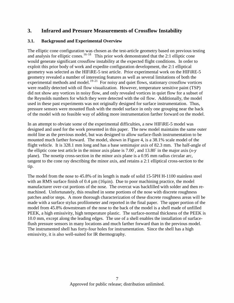
Kulite pressure transducers measured local static pressures. Additionally, several pressure transducers were operated in differential mode to measure differential pressures 180 degrees apart on the vehicle to aid in attitude determination. Details of the HIFiRE-5 pressure transducers are found in Reference 25. Although directly computed CFD results are available at each freestream condition only at 25 discrete values of α and β, they may be smoothly interpolated to provide computational pressure information at intermediate values of α and β as well. A similar approach, utilizing a matrix of CFD solution points, has recently been used for the implementation of Flush Air Data Sensing (FADS) algorithms for reconstructing the Mars Science Laboratory entry, descent, and landing trajectory.31 These interpolated CFD p values at the locations of 15 pressure transducers are calculated. The percentage root mean square differences between the set of transducers and the CFD results are presented in Figure 23 for the M=2.51 case. Results are shown for 15 pressure transducers distributed circumferentially around the HIFiRE-5 surface at t = 18.4827s. The RMS value is minimized at the value of α and β where the interpolated CFD results are most like the flight data. This minimum is indicated with a white dot. The IMU value for the same time is indicated with a white ×.The RMS value is minimized at the value of α and β where the interpolated CFD results are most like the flight data, and this reconstructed angle of attack and yaw information is compared to the recorded IMU trajectory data from the same point in time. Good agreement is found for all three inflow conditions.
29 Approved for public release; distribution unlimited.
Figure 23 Contour Plot of Percent RMS Differences between the Interpolated Pressure
CFD and the Measured Pressure at t = 18.4827s
It was infeasible to perform an array of 25 CFD cases for each time-step in the flight data set. However, normalizing each of the 25 cases for the three available pressure CFD conditions with p∞ permits interpolations in Mach number to produce synthetic CFD results at time points other than the three discrete trajectory points for which CFD was actually performed. The RMS minimization procedure described above is then performed at each timepoint (at intervals of 0.01 s) for which there is sufficient pressure data over the entire ascent and reentry trajectory. These reconstructed results, when correlated with the IMU results for α and β from the flight, show excellent agreement for the entirety of the ascent and reentry portions of the trajectory. Results from the ascent portion of the flight are presented in Figure 24. While the amplitude of α and β cyclic oscillations found in the reconstructed trajectory are larger in the IMU data for the first portion of the ascent, good agreement with the mean values is observed, and excellent agreement with both the mean and oscillating α and β values for the latter portion of the ascent. Good agreement is also observed for the frequency of oscillation in both data sets.

30 Approved for public release; distribution unlimited.
Figure 24 AoA and Yaw Results for the Ascent Portion of the Trajectory from the
Interpolation/RMS Minimization Routine Compared with the IMU Values (The trajectory times corresponding to the three computed CFD cases are indicated by the dashed black
vertical lines on each plot.)
This analysis of the vehicle attitude, inferred independently from pressure measurements, increases confidence in the attitude inferred from the IMU and GPS. This was the first HIFiRE flight using this GPS and IMU. The analysis indicates that, at least over these flight times and conditions, the GPS and IMU were able to measure vehicle attitude within 1 degree, with agreement generally better than that. The final version of this paper will include an estimate

31 Approved for public release; distribution unlimited.
of the error associated with the payload attitude measurements, and additional analysis of attitude based on differential pressures.
4.4. Heat Transfer Distribution Analysis and Comparison with CFD
The primary aerothermal instrumentation for HIFiRE-5 consisted of Medtherm Corporation coaxial thermocouples. The values for heat flux q̇ presented in this work were calculated, under an adiabatic assumption for the back-face temperature, from the front-face thermocouple temperatures by solving the transient 1-D heat equation. The FORTRAN QCALC subroutine was translated to Matlab for this purpose. QCALC assumes one- dimensional heat transfer and uses a second-order Euler explicit finite difference approximation to solve for the temperature distribution through the vehicle shell; heat flux is obtained from a second-order approximation to the derivative of the temperature profile at the outer surface.32
Laminar and turbulent heat transfer calculations at the three time points described in Section 4.2 were normalized by Stanton number based on the wall and stagnation temperatures:
𝑆𝑆𝑆𝑆 =�̇�𝑞
(𝑇𝑇0 − 𝑇𝑇𝑤𝑤)𝜌𝜌∞𝑢𝑢∞𝐶𝐶𝑝𝑝
Stagnation temperature is used in the data reduction, since it is easier to define than recovery temperature, and wall temperatures were well away from recovery temperatures. As described in Section 4 . 3 for the pressure results normalized by p∞, this St normalization permits α- and β-dependent interpolations in Mach number to produce synthetic laminar and turbulent heat transfer CFD results at time points other than the three discrete trajectory points for which CFD was actually performed. This analysis is performed (at intervals of 0.01s) at every time point for which there is sufficient heat transfer data over the entire ascent and reentry trajectory. Results for the location of one thermocouple (x=0.8m, φ=90o), from which the time of laminar-turbulent transition at this location may be inferred, are presented in Figure 25.
The results in Figure 25 indicate good agreement between the measured and computed heat transfer, both taken at the location of one thermocouple. Note that small values for heat transfer at the beginning of reentry result in large variation, for a given experimental uncertainty, in St terms. Laminar to turbulent transition is clearly observed in this location at t = 197s. The oscillations in the interpolated CFD curves are the result of changing angle of attack and yaw. Continued analysis, to be presented in the final version of this paper, will include assessment of the measured and computed heating uncertainties, and a reassessment of transition times and Reynolds numbers, as based on computed heating rates.

32 Approved for public release; distribution unlimited.
Figure 25 Computed Laminar and Turbulent Heat Transfer Results for the Reentry
Portion of the Trajectory Combined with Flight Data (Left: Stanton number, right: dimensional variables.)
4.5. Axisymmetric Shell Heat Conduction Computations
Although measured heat transfer generally agreed well with computed heat transfer, some discrepancies existed, especially at lower heating levels. Since the heat transfer data reduction used a one-dimensional conduction assumption, it was possible that some discrepancies arose from multi-dimensional conduction effects. In order to investigate this, the TOPAZ unsteady conduction code was used to assess multi-dimensional heating. TOPAZ had been used previously to examine lateral conduction effects, but realistic heating distributions were not available when this prior effort was accomplished.25
The methodology for this analysis was to calculate time-dependent heating temperatures in the aeroshell, including convective heating and conduction, and then analyze these temperatures as if they were experimental thermocouple data. In this way, the input convective heating would be exactly known, and the heating rates inferred from the computed shell temperatures would be subject to realistic conduction effects. The computed PNS convective heat transfer rates served as convective boundary conditions to TOPAZ. TOPAZ calculations then provided the outer and inner surface aeroshell temperatures. These computed temperatures then served as inputs to the same QCALC inverse solver that was used to derive heat transfer from the flight thermocouple data. This analysis thus provided a semi-quantitative assessment of lateral conduction errors in the flight data analysis.
This analysis was semiquantitative for two reasons. First, the actual flight heating was unknown. The computed convective heating however, was at least a plausible approximation of flight heating. Secondly, only a 2D/axisymmetric version of TOPAZ was available, and turbulent-laminar transition was only approximately modeled. Nevertheless, separate calculations could approximate axial and circumferential conduction effects. These

33 Approved for public release; distribution unlimited.
approximations were not objectionable, since the objective of the study was not to recreate or calibrate the data reduction, but to provide some bounds on lateral conduction errors.
In the current study, the aeroshell was modeled first as an elliptic cylinder to model circumferential conduction. The grid for this analysis was a 90o arc of an elliptic cylinder with the same dimensions as HIFiRE-5 at x=400mm. Computed heat transfer rates were applied as convective boundary conditions on the outer surface of the shell. Transition was modeled as a simple step change from turbulent to laminar heating at the appropriate time at each angular location. The flight data in some cases displayed multiple excursions between fully laminar and fully turbulent heating over a period of time during transition. Given the approximate nature of the analysis, this was not deemed to be a significant source of error. In the second step of the analysis, a streamwise section of a 7o circular cone was used to model axial conduction. Streamwise centerline and leading edge heating distributions were imposed as boundary conditions in two separate calculations. The backface boundary condition was adiabatic in all cases.
Figure 26 shows isotherms for the elliptic cylinder at x=400mm for t=20 seconds, near the time of maximum ascent heating, and t=32 seconds, when convective heating had dropped sharply. At t=20 seconds, the dominant temperature gradient is normal to the surface, indicating that the assumption of 1D conduction into the aeroshell was largely valid. By t=32 seconds, the dominant temperature gradient is in the circumferential direction, indicating that lateral conduction at this time likely dominated over convective heating and conduction into the shell.
Figure 26 Measured and Computed Temperature History near the HIFiRE-5 Leading
Edge at x=400 mm
Figure 27 compares the input and derived heating histories for the elliptic cylinder at the centerline (φ=0o) and leading edge (φ=90o). The green lines indicate the heating rates that were input to TOPAZ as convective boundary conditions. The red lines indicate the heating rates that were inferred using the QCALC inverse solver, with the TOPAZ-calculated temperature histories as input. The effect of circumferential conduction is apparent at both locations.
yy
z z
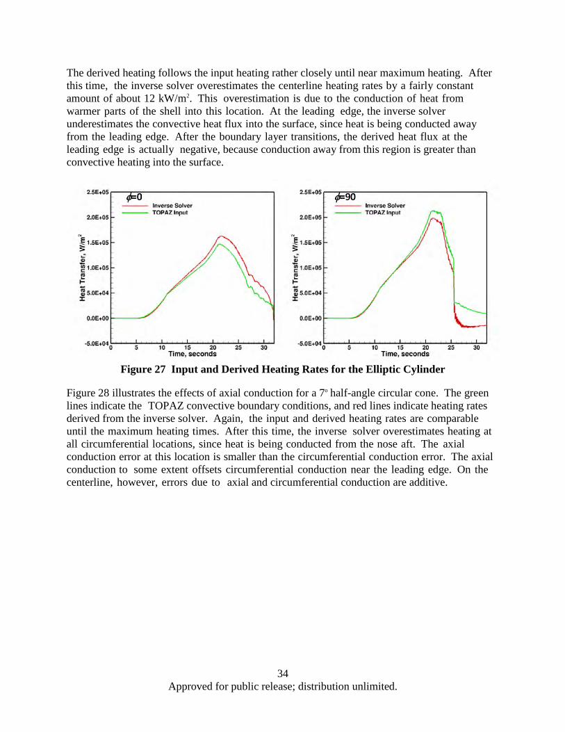
34 Approved for public release; distribution unlimited.
The derived heating follows the input heating rather closely until near maximum heating. After this time, the inverse solver overestimates the centerline heating rates by a fairly constant amount of about 12 kW/m2. This overestimation is due to the conduction of heat from warmer parts of the shell into this location. At the leading edge, the inverse solver underestimates the convective heat flux into the surface, since heat is being conducted away from the leading edge. After the boundary layer transitions, the derived heat flux at the leading edge is actually negative, because conduction away from this region is greater than convective heating into the surface.
Figure 27 Input and Derived Heating Rates for the Elliptic Cylinder
Figure 28 illustrates the effects of axial conduction for a 7o half-angle circular cone. The green lines indicate the TOPAZ convective boundary conditions, and red lines indicate heating rates derived from the inverse solver. Again, the input and derived heating rates are comparable until the maximum heating times. After this time, the inverse solver overestimates heating at all circumferential locations, since heat is being conducted from the nose aft. The axial conduction error at this location is smaller than the circumferential conduction error. The axial conduction to some extent offsets circumferential conduction near the leading edge. On the centerline, however, errors due to axial and circumferential conduction are additive.

35 Approved for public release; distribution unlimited.
Figure 28 Input and Derived Heating Rates for the Circular Cone at x=400 mm
Of the three vehicle stations where thermocouples were arrayed around the circumference, the x=400 mm station would have possessed the maximum axial and circumferential conduction errors, since the temperature gradients were at a maximum. This analysis indicates that near the centerline, flight heating rates were overestimated at t=25 seconds by approximately 27 kW/m2. On the leading edge at this time, flight heating rates would have been underestimated by about 16 kW/m2. During reentry, lateral conduction errors would have been less since the payload temperature had largely equilibrated prior to reentry, minimizing temperature gradients in both directions. This analysis is only approximate in nature, but it indicates the feasibility of more sophisticated thermal analysis of configurations like HIFiRE-5, either using a 3D inverse solver, or multiple iterations with a 3D unsteady conduction solver.
4.6. Conclusions
It has been demonstrated that normalized pressure CFD results may be used to infer angle of attack and yaw from a set of pressure transducers distributed over the body of the HIFiRE-5 flight test article. Interpolations in Mach number have been correlated with the Inertial Measurement Unit results for α and β from the flight, with excellent agreement for the entirety of the ascent and reentry portions of the trajectory. A similar normalization of the laminar and turbulent heat transfer CFD results with St has been compared to flight heat transfer measurements, and transition locations have been inferred. Computational heat conduction analysis has demonstrated that the assumptions inherent in the calculation of heat flux from temperature are reasonable for much of the HIFiRE-5 trajectory, and may account for discrepancies between measured and computed laminar and turbulent heat transfer levels. If so, further work to characterize lateral and axial conduction would enable a correction factor to be applied to the thermocouple-derived measurement of q̇ for the portions of the trajectory where this effect is significant.
The analysis presented in this paper indicates that is feasible to reconstruct the HIFiRE-5 flight using a synthesis of measured and computed data. It may be possible to extend this type of analysis to future flights of HIFiRE and other hypersonic vehicles.

36 Approved for public release; distribution unlimited.
5. Boundary Layer Stability Analysis for Stetson’s Mach 6 Blunt Cone Experiments
5.1. Background
Between 1978 and 1982, K. F. Stetson performed a total of 196 sharp- and blunt-cone experiments on an 8o half-angle, 4 in. base cone in the Air Force Research Laboratory Mach 6 High Reynolds Number facility.33 These experiments were reported in a 1983 paper along with results from AEDC Tunnel F with a larger cone at Mach 9.34 While the AEDC Mach 9 results have received computational analysis,35 the AFRL Mach 6 results have not, to date.
The AFRL Mach 6 facility operates at stagnation pressure p0 from 700 to 2100 psi. Presently, computations for three representative conditions spanning the operating envelope have been completed. These conditions, which are presented in Table 3, cover 34 out of the 196 experiments33 and cover a significant portion of the Stetson Mach 6 results34 (see Section 5.3). Computations for the remaining 162 experiments, which actually encompass only 88 independent simulations due to repeated conditions, are underway and on the present computational setup are completed at a rate of about 6 per 24 hours.
Table 3 Summary of Inflow Conditions Computed for Each Bluntness Value
[psi]
p0
[MPa] unit Re∞
×106/m M∞
- ρ∞
[kg/m3] P∞
[kPa] T∞
[K] U∞
[m/s] Tw/T0
- 700 4.83 30.7 5.9 0.154 3.40 76.7 1038 0.56
1400 9.65 61.4 5.9 0.308 6.80 76.7 1038 0.56 2100 14.5 92.1 5.9 0.461 10.2 76.7 1038 0.56
5.2. Computational Methods
The mean flow over the cone is computed by the reacting, axisymmetric Navier-Stokes equations with a structured grid, using a version of the NASA Data Parallel-Line Relaxation (DPLR)36 code which is included as part of the STABL software suite, as described by Johnson37 and Johnson et al.38 This flow solver is also based on the finite-volume formulation. The use of an excluded volume equation of state is not necessary for the boundary layer solver because the static pressure over the cone is sufficiently low (typically, 10–50 kPa) that the gas can be treated as ideal. The mean flow is computed on a single-block, structured grid (see Figure 29) with dimensions of 361 cells by 359 cells in the streamwise and wall-normal directions, respectively. Grids for the sharp 8 o half-angle cone and each of the 10 bluntness conditions (see Table 4) were generated using STABL’s built-in grid generator, and mean flow solutions examined to ensure that at least 100 points were placed in the boundary layer for each stagnation pressure. The boundary-layer profiles and edge properties are extracted from the mean flow solutions during post-processing. The wall-normal span of the grid increases down the length of the cone, from 0.25 mm at the tip to 50 mm at the base, allowing for the shock to be fully contained within the grid for all cases tested. The grid is clustered at the wall as well as at the nose in order to capture the gradients in these locations. The Δy+ value for the grid, extracted from the DPLR solution for each

37 Approved for public release; distribution unlimited.
case, is everywhere less than 1, where Δy+ is a measure of local grid quality at the wall in the wall-normal direction.
Figure 29 Grid for the Sharp Cone Case with 361 Streamwise and 359 Wall-normal Cells
(For clarity, every fifth wall-normal cell is shown.)
Table 4 Summary of Grids Generated for the Present Study, Each Corresponding to a Different Sharp or Blunt Nosetip Used by Stetson
rN
in. mm Bluntness
% 0 0 0.02 0.508 0.04 1.016 0.06 1.524 0.08 2.032 0.10 2.540 0.20 5.080 0.30 7.620 0.40 10.16 0.50 12.70 0.60 15.24
0 1 2 3 4 5
10 15 20 25 30
Stetson34 reported results by “normalizing” the transition Reynolds numbers for blunted cones by the transition Reynolds numbers for sharp cones at the same inflow conditions, which are calculated as:
𝑋𝑋𝑇𝑇𝑇𝑇𝐵𝐵𝑋𝑋𝑇𝑇𝑇𝑇𝑠𝑠
=(𝑅𝑅𝑅𝑅𝑋𝑋)𝑇𝑇𝑇𝑇𝐵𝐵(𝑅𝑅𝑅𝑅𝑋𝑋)𝑇𝑇𝑇𝑇𝐵𝐵
(𝑅𝑅𝑅𝑅𝑢𝑢𝑢𝑢𝑢𝑢𝑢𝑢)𝑒𝑒𝑆𝑆(𝑅𝑅𝑅𝑅𝑢𝑢𝑢𝑢𝑢𝑢𝑢𝑢)𝑒𝑒𝐵𝐵
Here, subscript “S” indicates values for a sharp tip, “B” values for a given blunt tip at the same condition, and “e” conditions at the boundary layer edge. Stetson34 performed selected computations with two boundary layer codes and used some interpolations to find the unit Reynolds number and Mach number at the boundary layer edge and throughout the entropy layer, but notes that “it was not considered practical to make boundary layer calculations for all of the geometric and flow variations of the present investigation.” This is now possible; two examples for a sharp and blunt case are presented in Figure 30. The swallowing length estimate
x
z

38 Approved for public release; distribution unlimited.
of Rotta39 is also used to correlate the results. While the freestream unit Reynolds number is 61.4×10⁶/m for both cases, the large “swallowing length” of the blunt case is evident.
Figure 9 in Stetson34 summarizes his results, and is digitized from Stetson33 below as Figure 31 and Figure 32, with the cases already computed shown as red solid circles, and the other cases shown as blue hollow circles.
Figure 30 Sharp and Blunt Unit Reynolds Number Contours (detail) for the p0 = 1400 psi
Inflow Case
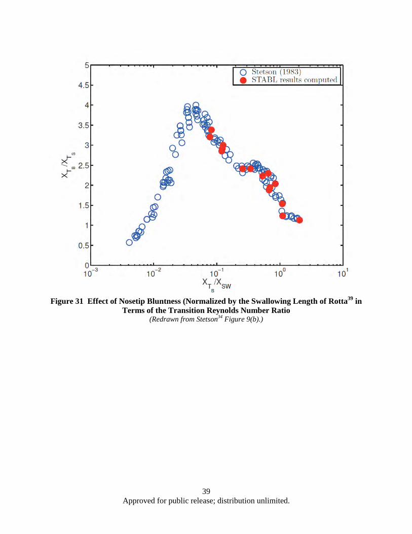
39 Approved for public release; distribution unlimited.
Figure 31 Effect of Nosetip Bluntness (Normalized by the Swallowing Length of Rotta39 in
Terms of the Transition Reynolds Number Ratio (Redrawn from Stetson34 Figure 9(b).)

40 Approved for public release; distribution unlimited.
Figure 32 Effect of Nosetip Bluntness (Normalized by the Swallowing Length of Rotta7 in
Terms of the Transition Reynolds Number Ratio (Redrawn from Stetson34 Figure 9(b).)
5.3. Stability Computations
The stability analyses are performed using the PSE-Chem solver, which is also part of the STABL software suite. PSE-Chem40 solves the reacting, two-dimensional, axisymmetric, linear parabolized stability equations (PSE) to predict the amplification of disturbances as they interact with the boundary layer. The PSE-Chem solver includes finite-rate chemistry and translational-vibrational energy exchange. The parabolized stability equations predict the amplification of disturbances as they interact with the boundary layer.
The band of amplified frequencies within the boundary layer is presented on contour plots in terms of amplification −αi in Figure 33. The most amplified frequency predicted by a simple model based on edge velocity and boundary layer thickness is also plotted for each case, and shows generally good agreement with the detailed computations.
For the cases computed so far (i.e., for the red circles in Figure 31 and Figure 32), computed N-factors at the experimental transition location are presented in Figure 34. Note that the sharp data points are located at infinity on the x-axis and appear to be the asymptotic value for N-factor at transition with decreasing nose tip bluntness.

41 Approved for public release; distribution unlimited.
Figure 33 LST Contours of −αi for rN = 1.016 mm (2%) for the p0 = 1400 psi Inflow
Condition

42 Approved for public release; distribution unlimited.
Figure 34 Computed N-factor at Experimental Transition Location Reported in Stetson33, 34
A strong trend in transition N-factor for both nose tip bluntness and swallowing length ratio is observed in the results computed so far (see Figure 34), which cover a substantial portion of the Stetson conditions.34 The remaining conditions will be computed at a later date. As bluntness increases and the calculated swallowing distance lengthens, the computed N-factor at the experimentally-observed transition location drops below the level at which Mack’s second mode would be expected to lead to transition.41, 42 These results indicate that the dominant instability mechanism for the bluntest cases is likely not the second mode.
Based upon the computed second-mode amplification factors eN , transition onset in the AFRL Mach 6 High Reynolds Number facility is estimated to correspond to N ≈ 7 for the sharp and nearly sharp cases. These amplification values are high as compared to the more typical value of N ≈ 5–6 usually characterizing a “noisy” tunnel.43 However, recent results have found relatively high transition N-factors in noisy tunnels for cases where there is a mismatch between the strongest free stream noise frequencies and the most unstable boundary-layer frequencies.44- 46 Measurements of free stream instability in the Mach 6 tunnel would be essential for confirming whether this is the case in the present study.

43 Approved for public release; distribution unlimited.
6. HIFiRE-1 Turbulent Shock Boundary Layer Interaction – Flight Data and Computations
6.1. Background
HIFiRE-1 launched 22 March 2010 at the Woomera Prohibited Area in South Australia at 0045UTC (1045 local time). The primary objective of HIFiRE-1 was to measure aerothermal phenomena in hypersonic flight. The primary experiment consisted of boundary-layer transition measurements on a 7-deg half angle cone with a 2.5 mm radius nose. The secondary aerothermal experiment was a shock-boundary-layer interaction created by a 33-deg-flare / cylinder configuration. HIFiRE-1 ground test and computation created an extensive knowledge base regarding transition and SBLI on axisymmetric bodies. This research has been summarized in numerous prior publications.47,48,49,50,51,52,53,54,55,56,57
Preliminary results from the HIFiRE-1 aerothermal experiments have been previously published.58 Ref. 58 presented preliminary results from both the BLT and SBLI experiments during ascent and descent. Although the vehicle was at a higher angle of attack than intended during descent, the payload instrumentation scheme permitted acquisition of interesting and useful high angle-of-attack (AoA) transition data. 59,60 Analysis of the high AoA reentry SBLI experiment is considerably more difficult, so the current paper focuses only on the ascent-phase SBLI. A prior publication expanded on the SBLI experiment focused on unsteady pressure measurements.61 The current publication focuses on comparing computations of the SBLI to flight measurements for the ascent phase of flight.
HIFiRE-1 presents an unusual test case for CFD, since highly-detailed surface measurements were made on a relatively simple configuration. Although the flight conditions were relatively benign, with a maximum Mach number of seven during reentry, computation of the turbulent SBLI is not trivial. Although CFD codes can be calibrated against wind tunnel results prior to applying them to flight conditions, it is generally not possible to match flight conditions exactly in ground test. HIFiRE-1 showed significant variations in flight conditions and wall temperatures during ascent. Freestream unit Reynolds numbers ranged from 0 to 60x106 per meter during ascent, and ascent Mach number varied from subsonic to approximately 5.5. Flare temperatures ranged from approximately 300 K to a peak of 540 K during ascent, and at any time varied significantly through the interaction. Computation of the HIFiRE-1 ascent turbulent SBLI provides an interesting test of a computer code calibrated against a point condition in a wind tunnel.
The HIFiRE-1 vehicle has been described in several prior publications, most notably in Ref. 57. The overall payload dimensions and the different payload modules are shown in Fig. 35. The experiments were carried out on the forward sections of the payload including a cone, a cylinder, and a flare that transitioned to the diameter of the second stage motor (0.356 m). The nose tip consisted of an iridium-coated, titanium-zirconium-molybdenum (TZM) alloy. The surface finish of the nose tip after coating was measured to be 6-8 microinches (0.15-0.2 microns) RMS (root mean square). The aluminum cone shell was finished to a 0.8 micron Ra finish (Ra is the arithmetic average of roughnesses). The cone half angle of seven degrees was chosen to match configurations used in preceding ground tests and analytical/numerical work. The aft-portion of the cylinder and the flare consisted of AISI 1045 steel.

44 Approved for public release; distribution unlimited.
The payload contained duplicate instrumentation on rays 180o apart, permitting a cross-check between instrumentation on these two rays. One ray of instrumentation contained a diamond-shaped trip to produce a roughness-induced transition. The payload incorporated this feature to ensure that turbulent data might be obtained even if the reentry portion of the flight terminated before natural transition occurred. Pressures and temperatures on the flare on this ray were recorded throughout flight. The circuit board that conditioned SBLI pressures on the cylinder on this ray failed at approximately t=6 seconds, therefore no data were recorded from these instruments after this time.
The ray of instrumentation 180o opposite of the trip contained no intentional trip element. However, backward-facing steps on the nosetip of the vehicle tripped transition for t<11.5 seconds. For t>11.5 seconds, transition moved aft with time over the conical portion of the vehicle, until about t=21.5 seconds. At this point, flow over the cone was entirely laminar. The SBLI began to take on characteristics of a transitional interaction at about this time.
Figure 35 HIFiRE-1 Payload Configuration, Dimensions in mm
The payload flew a ballistic trajectory similar to those employed for the HyShot62 and
Hypersonic Collaborative Australia/United States Experiment (HyCAUSE)63 flights. The as-
flown trajectory is shown in Fig. 36. The Terrier first stage burnt for 6.3 seconds and was then drag-separated from the second stage. The Orion/payload combination coasted until the second stage ignited at 15 seconds. Orion burnout occurred at 43 seconds. The payload remained attached to the second stage throughout the entire flight to provide stability as the payload
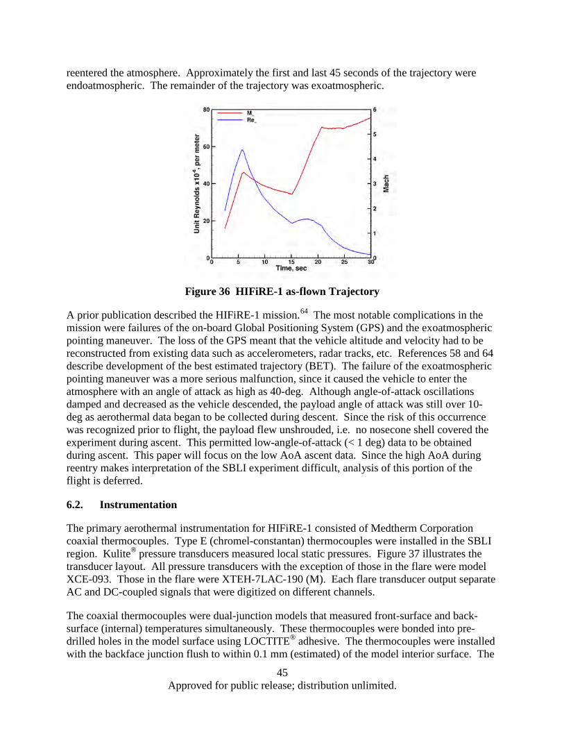
45 Approved for public release; distribution unlimited.
reentered the atmosphere. Approximately the first and last 45 seconds of the trajectory were endoatmospheric. The remainder of the trajectory was exoatmospheric.
Figure 36 HIFiRE-1 as-flown Trajectory
A prior publication described the HIFiRE-1 mission.64 The most notable complications in the mission were failures of the on-board Global Positioning System (GPS) and the exoatmospheric pointing maneuver. The loss of the GPS meant that the vehicle altitude and velocity had to be reconstructed from existing data such as accelerometers, radar tracks, etc. References 58 and 64 describe development of the best estimated trajectory (BET). The failure of the exoatmospheric pointing maneuver was a more serious malfunction, since it caused the vehicle to enter the atmosphere with an angle of attack as high as 40-deg. Although angle-of-attack oscillations damped and decreased as the vehicle descended, the payload angle of attack was still over 10-deg as aerothermal data began to be collected during descent. Since the risk of this occurrence was recognized prior to flight, the payload flew unshrouded, i.e. no nosecone shell covered the experiment during ascent. This permitted low-angle-of-attack (< 1 deg) data to be obtained during ascent. This paper will focus on the low AoA ascent data. Since the high AoA during reentry makes interpretation of the SBLI experiment difficult, analysis of this portion of the flight is deferred.
6.2. Instrumentation
The primary aerothermal instrumentation for HIFiRE-1 consisted of Medtherm Corporation coaxial thermocouples. Type E (chromel-constantan) thermocouples were installed in the SBLI region. Kulite® pressure transducers measured local static pressures. Figure 37 illustrates the transducer layout. All pressure transducers with the exception of those in the flare were model XCE-093. Those in the flare were XTEH-7LAC-190 (M). Each flare transducer output separate AC and DC-coupled signals that were digitized on different channels.
The coaxial thermocouples were dual-junction models that measured front-surface and back-surface (internal) temperatures simultaneously. These thermocouples were bonded into pre-drilled holes in the model surface using LOCTITE® adhesive. The thermocouples were installed with the backface junction flush to within 0.1 mm (estimated) of the model interior surface. The

46 Approved for public release; distribution unlimited.
portion of the thermocouple which extended beyond the model external surface was removed using files and abrasives so that the final thermocouple contour matched the model surface contour. This finishing process created a “sliver junction” between the center-wire and annular thermocouple materials, in which whiskers of one conductor are dragged over the other to create the thermocouple junction.
Figure 37 SBLI Transducer Layouts
6.3. Computations
The computations proceeded in two stages. The first stage of computations consisted of calculations for test results from the CUBRC LENS wind tunnel. This permitted several
PLBW Flare
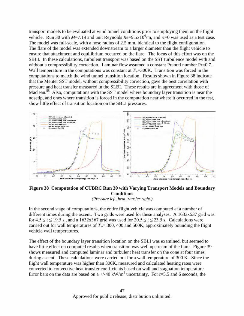
47 Approved for public release; distribution unlimited.
transport models to be evaluated at wind tunnel conditions prior to employing them on the flight vehicle. Run 30 with M=7.19 and unit Reynolds Re=9.5x10⁶/m, and α=0 was used as a test case. The model was full-scale, with a nose radius of 2.5 mm, identical to the flight configuration. The flare of the model was extended downstream to a larger diameter than the flight vehicle to ensure that attachment and equilibrium occurred on the flare. The focus of this effort was on the SBLI. In these calculations, turbulent transport was based on the SST turbulence model with and without a compressibility correction. Laminar flow assumed a constant Prandtl number Pr=0.7. Wall temperature in the computations was constant at Tw=300K. Transition was forced in the computations to match the wind tunnel transition location. Results shown in Figure 38 indicate that the Menter SST model, without compressibility correction, gave the best correlation with pressure and heat transfer measured in the SLBI. These results are in agreement with those of Maclean.55 Also, computations with the SST model where boundary layer transition is near the nosetip, and ones where transition is forced in the computation near where it occurred in the test, show little effect of transition location on the SBLI pressures.
Figure 38 Computation of CUBRC Run 30 with Varying Transport Models and Boundary Conditions
(Pressure left, heat transfer right.)
In the second stage of computations, the entire flight vehicle was computed at a number of different times during the ascent. Two grids were used for these analyses. A 1633x537 grid was for 4.5 ≤ t ≤ 19.5 s., and a 1632x367 grid was used for 20.5 ≤ t ≤ 23.5 s. Calculations were carried out for wall temperatures of Tw= 300, 400 and 500K, approximately bounding the flight vehicle wall temperatures.
The effect of the boundary layer transition location on the SBLI was examined, but seemed to have little effect on computed results when transition was well upstream of the flare. Figure 39 shows measured and computed laminar and turbulent heat transfer on the cone at four times during ascent. These calculations were carried out for a wall temperature of 300 K. Since the flight wall temperature was higher than 300K, measured and calculated heating rates were converted to convective heat transfer coefficients based on wall and stagnation temperature. Error bars on the data are based on a +/-40 kW/m2 uncertainty. For t=5.5 and 6 seconds, the

48 Approved for public release; distribution unlimited.
measured heat transfer correlates well with predicted turbulent values. For t=15.5 and 21.5 seconds, the transition from laminar to turbulent heating on the cone is apparent.
Even though the cone contains a region of turbulent flow over its aft portion at t=21.5 seconds, measurements on the smooth-side SBLI begin to deviate from the tripped side slightly before this time. This departure is evident in Figure 40, which shows smooth and rough-side temperatures on the first transducer on the flare downstream of the corner. Temperatures on both sides of the payload agree well until t=20 seconds. At this point, temperatures on the smooth side begin to rise and spike at approximately t=22 seconds. After this, temperatures decay. It is surmised that this behavior was due to the transitional nature of the flow over the smooth side of the payload. Therefore, comparisons between measured and computed SBLI quantities will be constrained to times less than 20 seconds when transition occurs well upstream on the cone.
Figure 39 Measured and Computed Cone Heat Transfer at Various Times
Conv
ectio
n Co
effic
ient
h, W
/m2 /
KCo
nvec
tion
Coef
ficie
nt h
, W/m
2 /K
Conv
ectio
n Co
effic
ient
h, W
/m2 /
KCo
nvec
tion
Coef
ficie
nt h
, W/m
2 /K
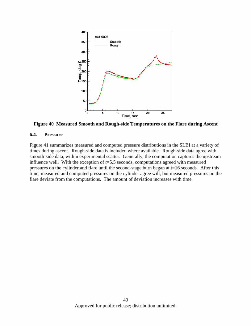
49 Approved for public release; distribution unlimited.
Figure 40 Measured Smooth and Rough-side Temperatures on the Flare during Ascent
6.4. Pressure
Figure 41 summarizes measured and computed pressure distributions in the SLBI at a variety of times during ascent. Rough-side data is included where available. Rough-side data agree with smooth-side data, within experimental scatter. Generally, the computation captures the upstream influence well. With the exception of t=5.5 seconds, computations agreed with measured pressures on the cylinder and flare until the second-stage burn began at t=16 seconds. After this time, measured and computed pressures on the cylinder agree will, but measured pressures on the flare deviate from the computations. The amount of deviation increases with time.

50 Approved for public release; distribution unlimited.
Figure 41 Measured and Computed SBLI Pressure Distributions during Ascent
Several possible causes for the large flare pressure overshoots during second-stage burn were examined. The pressure transducers were temperature and acceleration-compensated, so the increased flare temperature or the acceleration during boost was unlikely to have produced the overshoot. Also, even though the Orion second-stage thrust dropped at about 19.3 seconds as the motor entered a sustain-burn phase, causing the payload axial acceleration to drop, the flare pressure overshoot remained high. The temperature boundary condition was examined as another possible cause. Figure 42 shows the effect of increasing the surface temperature from 300 K to 500 K in the computation. As expected, this has little effect on the surface pressures. Increased temperature causes a slight reduction in the computed surface pressure. The increased temperature causes a slight expansion of the upstream influence, probably due to the increase in boundary layer thickness attendant with the higher wall temperature.

51 Approved for public release; distribution unlimited.
Figure 42 Effect of Surface Temperature on SBLI Pressure
In order to understand the high pressures seen on the flare, the measured and computed pressures were compared to expected inviscid flare pressures. The inviscid flare pressures were derived from the Taylor-Maccoll solution for a 33o half-angle cone. For the times examined, the computations show undershoots of the inviscid pressure. For t≤17.5 seconds, the experimental data show either an undershoot or a modest overshoot of inviscid pressure. At later times, the measured pressures overshoot the inviscid levels by large amounts. Although some pressure overshoot is expected at reattachment in a SBLI, the measured flight pressures far exceed any overshoot amounts observed in ground test. For this reason, measured pressures on the flare for times greater than 17.5 seconds must be viewed with skepticism. Although some transitional effects may come into play for t≥20 seconds, the mechanism behind these large overshoots remains unknown. Therefore, it can only be concluded that the large pressure overshoots on the flare were spurious and non-physical. Although the transducers were temperature and acceleration compensated, it may be possible that some factors caused this compensation to be ineffective. Another possibility is that boost acceleration caused mechanical strain in the transducers, leading to erroneous results.
Pres
sure
, kPa
Pres
sure
, kPa
x, meters x, meters

52 Approved for public release; distribution unlimited.
Figure 43 Measured and Computed Pressures Compared to Expected Inviscid Flare
Pressures
6.5. Heat Transfer
Figure 44 illustrates the comparison between measured and computed heat transfer in the SBLI after first-stage burnout. Since the CFD was computed at a constant wall temperature, and the experimental wall temperatures varied in space and time, the heating is compared on the basis of the convective heat transfer coefficient, h. The convective heat transfer coefficient h is evaluated based on the measured or computed temperature and the stagnation temperature, ℎ =�̇�𝑞/(𝑇𝑇0 − 𝑇𝑇𝑤𝑤). Although the heat transfer coefficient is better evaluated using the recovery temperature, this quantity is difficult to evaluate, and the impact on heat transfer coefficient is minimal unless the wall temperature approaches the recovery temperature. The agreement between the measured and computed heat transfer is fair, and this is due mostly to the large scatter in the measured heat transfer. This is especially true for t=15 and 17.5 seconds, when the heating rates were very low.

53 Approved for public release; distribution unlimited.
Figure 44 Measured and Computed Heat Transfer
6.6. Conclusions and Future Work
The DPLR code using the SST turbulence model with no compressibility correction performed well in predicting the SBLI pressure and heat transfer over most of the HIFiRE-1 ascent. This performance is in agreement with expectations based on experimental / computational comparisons with ground tests at CUBRC at Mach 7. Flight data during the second-stage boost showed significant pressure overshoots on the flare. The mechanism behind these overshoots, or whether they are even physical or due to sensor malfunction, is unknown. Overall, the good agreement between the measured flight data and the computations helps to validate the strategy of calibrating CFD against wind tunnel tests prior to exercising codes at flight conditions.

54 Approved for public release; distribution unlimited.
7. References
1 Borg, M. P., “Simultaneous Infrared and Pressure Measurements of Crossflow Instability Modes for HIFiRE-5,” abstract submitted to AIAA Scitech 2016 meeting, January 2016.
2 Jewell, J. S. and Kimmel, R. L., “Boundary Layer Stability Analysis for Stetson’s Mach 6 Blunt Cone Experiments,” abstract submitted to AIAA Scitech 2016 meeting, January 2016.
3 Jewell, J. S., Miller, J. H., Kimmel, R. L., “Correlation of HIFiRE-5 Flight Data With Computed Pressure and Heat Transfer,” AIAA paper 2015-2019, June 2015.
4 Kimmel, R. L. and Prabhu, D., “HIFiRE-1 Turbulent Shock Boundary Layer Interaction –Flight Data and Computations,” AIAA paper 2015-2639.
5 Warwick, G., “Uncertain Flight – DARPA hopes more robust flight control will keep hypersonic HTV-2 on track,” Aviation Week and Space Technology, August 1, 2011, p. 14.
6 Gronvall, J. E., Bisek, N. J. and Poggie, J., “High Fidelity Computational Study of the HIFiRE-1 Boundary Layer Trip,” AIAA paper 2014-0433, January 2014.
7 Kimmel, R. L, Adamczak, D., Berger, K., and Choudhari, M., “HIFiRE-5 Flight Vehicle Design,” AIAA paper 2010-4985, June 2010.
8 Choudhari, M., Chang, C.-L., Jentink, T., Li, F., Berger, K., Candler, G., and Kimmel, R., “Transition Analysis for the HIFiRE-5 Vehicle,” AIAA paper 2009-4056, June 2009.
9 Gosse, R., Kimmel, R., “CFD Study of Three-Dimensional Hypersonic Laminar Boundary Layer Transition on a Mach 8 Elliptic Cone,” AIAA paper 2009-4053, June 2009.
10 Juliano, T. J., Schneider, S., “Instability and Transition on the HIFiRE-5 in a Mach 6 Quiet Tunnel,” AIAA paper 2010-5004, June 2010.
11 Paredes, P. and Theofilis, V., “Spatial linear global instability analysis of the HIFiRE-5 elliptic cone model flow,” AIAA paper 2014-0075, January 2014.
12 Paredes, P. and Theofilis, V., “Traveling Global instabilities on the HIFiRE-5 elliptic cone model flow,” AIAA paper 2013-2880, June 2013.
13 Huntley, M. B., “Transition on Elliptic Cones at Mach 8,” Ph. D. thesis, Princeton University Department of Mechanical and Aerospace Engineering, Princeton, NJ, November 2000.
14 Li, F., Choudhari, M., Chang, C.-L., Kimmel, R., Adamczak, D., and Smith, M., “Transition Analysis for the HIFiRE-1 Flight Experiment,” AIAA paper 2011-3414, June 2011.
15 Alba, C. R., Johnson, H. B., Bartkowicz, M. D., Candler, G. V., and Berger, K. T. “Boundary-Layer Stability Calculations for the HIFiRE-1 Transition Experiment,” AIAA Journal of Spacecraft and Rockets, vol. 45, no. 6, November-December 2008, pp. 1125-1133.
55 Approved for public release; distribution unlimited.
16 Kimmel, R. L. and Poggie, J., “Transition on an Elliptic Cone at Mach 8,” American Society of Mechanical Engineers ASME FEDSM97-3111, June 1997.
17 Kimmel, R. L. and Poggie, J. J., “Three-Dimensional Hypersonic Boundary Layer Stability and Transition,” WL-TR-97- 3111, Air Force Research Laboratory Technical Report, Wright-Patterson Air Force Base, Ohio, Dec. 1997.
18 Kimmel, R. L., Poggie, J. J., and Schwoerke, S. N., “Laminar-Turbulent Transition in a Mach 8 Elliptic Cone Flow,” AIAA Journal, Vol. 37, No. 9, September 1999, pp. 1080–1087.
19 Borg, M. P., Kimmel, R. L., and Stanfield, S., “Crossflow Instability for HIFiRE-5 in a Quiet Hypersonic Wind Tunnel,” Paper 2012-2821, AIAA, June 2012.
20 Borg, M. P., Kimmel, R. L., Hofferth, J. W., Bowersox, R. D., and Mai, C. L., “Freestream effects on boundary layer disturbances for HIFiRE-5,” Paper 2015-0278, AIAA, January 2015.
21 Borg, M. P., and Kimmel, R. L., “Traveling Crossflow Instability for the HIFiRE-5 Elliptic Cone,” AIAA Journal of Spacecraft and Rockets, vol. 52, no. 3, May-June 2015.
22 Schneider, S. P., “Design of a Mach-6 quiet-flow wind-tunnel nozzle using the e**N method for transition estimation,” AIAA paper 98-0547, January 1998.
23 Li, F., Choudhari, M., Chang, C.-L., White, J., Kimmel, R., Adamczak, D., Borg, M., Stanfield, S., and Smith, M., “Stability Analysis for HIFiRE Experiments,” AIAA paper 2012–2961, June 2012.
24 Beresh, S. J., Henfling, J., Spillers, R., and Pruett, B., “Measurements of Fluctuating Wall Pressures Beneath a Supersonic Turbulent Boundary Layer,” Paper 2010-0305, AIAA, January 2010.
25 Kimmel, R. L., Adamczak, D., Juliano, T. J., and the DSTO AVD Brisbane Team. “HIFiRE-5 Flight Test Preliminary Results,” AIAA Paper 2013-0377, January 2013.
26 Juliano, T. J., Adamczak, D., and Kimmel, R. L. “HIFiRE-5 Flight Test Heating Analysis,” AIAA paper 2014-0076, January 2014.
27 Miller, J.H., Adamczak, D.W., and Tancred, J.A., “Flight Data Reduction for HIFiRE Flight 5,” DCASS-129 presentation, Dayton-Cincinnati Aerospace Sciences Symposium, Dayton, OH, March 2013.
28 Tannehill, J.C., Miller, J.H., and Lawrence, S.L., “Development of an Iterative PNS Code for Separated Flows,” AIAA Paper 99-3361, June 1999.
29 Lawrence, S.L., Chaussee, D.S., and Tannehill, J.C., “Application of an Upwind Algorithm to the Three-Dimensional Parabolized Navier-Stokes Equations,” AIAA Journal, Vol. 28, No. 6, 1990, pp. 971,972.
30 Baldwin, B.S. and Lomax, H., “Thin Layer Approximation and Algebraic Model for Separated Turbulent Flows,” AIAA Paper 78-257, Jan. 1978.

56 Approved for public release; distribution unlimited.
31 Karlgaard, C. D., Kutty, P., Schoenberge, M., Munk, M. M., Little, A. and Kuhl, C. A., “Mars Science Laboratory Entry Atmospheric Data System Trajectory and Atmosphere Reconstruction,” AIAA Journal of Spacecraft and Rockets, vol. 51, no. 4, 2014, pp. 1029-1047.
32 Boyd, C. F. and Howell, A., “Numerical investigation of one-dimensional heat-flux calculations,” Technical Report NSWCDD/TR-94/114, Dahlgren Division Naval Surface Warfare Center, Silver Spring, MD 20903-5640, October 1994.
33 Stetson, K. F., “Notes related to previous AIAA papers on blunt cones,” Personal communication to S. P. Schneider, December 2001, Purdue University.
34 Stetson, K. F., “Nosetip Bluntness Effects on Cone Frustum Boundary Layer Transition in Hypersonic Flow,” Proceedings of the AlAA 16th Fluid and Plasma Dynamics Conference, AIAA-83-1763, Danvers, Massachusetts, 1983.
35 Robarge, T. W. and Scheider, S. P., Laminar boundary-layer instabilities on hypersonic cones: Computations for benchmark experiments, AIAA-2005-5024, Toronto, ON, 2005.
36 Wright, M. J., Candler, G. V., and Bose, D., “Data-parallel line relaxation method for the Navier-Stokes equations,” AIAA Journal, Vol. 36, No. 9, 1998, pp. 1603–1609.
37 Johnson, H. B., Thermochemical Interactions in Hypersonic Boundary Layer Stability, Ph.D. thesis, University of Minnesota, Minneapolis, MN, 2000.
38 Johnson, H. B., Seipp, T. G., and Candler, G. V., “Numerical study of hypersonic reacting boundary layer transition on cones,” Physics of Fluids, vol. 10, 1998, pp. 2676–2685.
39 Rotta, N. R., “Effects of nose bluntness on the boundary layer characteristics of conical bodies at hyp2703ersonic speeds,” New York University Report NYUAA-66-66, 1966.
40 Johnson, H. B. and Candler, G. V., “Hypersonic boundary layer stability analysis using PSE-Chem,” 35th Fluid Dynamics Conference and Exhibit, AIAA, 2005, AIAA-2005-5023.
41 Fedorov, A. V., “Receptivity of a High-Speed Boundary Layer to Acoustic Disturbances,” Journal of Fluid Mechanics, vol. 491, 2003, pp. 101–129.
42 Fedorov, A. and Tumin, A., “High-Speed Boundary-Layer Instability: Old Terminology and a New Framework,” AIAA Journal, vol. 49, 2011, pp. 1647–1657.
43 Schneider, S. P., “Effects of High-Speed Tunnel Noise on Laminar-Turbulent Transition,” AIAA Journal of Spacecraft and Rockets, vol. 38, no. 3, 2001, pp. 323–333.
44 Jewell, J. S., Wagnild, R. M., Leyva, I. A., Candler, G. V., and Shepherd, J. E., “Transition Within a Hypervelocity Boundary Layer on a 5-Degree Half-Angle Cone in Air/CO2 Mixtures,” 51st AIAA Aerospace Sciences Meeting including the New Horizons Forum and Aerospace Exposition, AIAA-2013-0523, Grapevine, TX, 2013.
45 Jewell, J. S., Boundary-Layer Transition on a Slender Cone in Hypervelocity Flow with Real Gas Effects, Ph.D. thesis, California Institute of Technology, Pasadena, CA, 2014.
46 Parziale, N. J., Jewell, J. S., Leyva, I. A., and Shepherd, J. E., “Effects of Shock-Tube Cleanliness on Slender-Body Hypersonic Instability and Transition Studies at High Enthalpy,”

57 Approved for public release; distribution unlimited.
Proceedings of 53rd AIAA Aerospace Sciences Meeting, AIAA-2015-1786, Orlando, FL, 2015.
47 Kimmel, R. L., Adamczak, D., Gaitonde, D., Rougeux, A., Hayes, J. R., “HIFiRE-1 Transition Experiment Design,” AIAA paper 2007-0534, January 2007.
48 Wadhams, T. P., MacLean, M. G., Holden, M.S., and Mundy, E., “Pre-Flight Ground Testing of the Full-Scale FRESH FX-1 at Fully Duplicated Flight Conditions,” AIAA paper 2007-4488, June 2007.
49 Johnson, H. B., Alba, C. R., Candler, G. V., MacLean, M., Wadhams, T, and Holden, M. “Boundary Layer Stability Analysis of the Hypersonic International Flight Research Transition Experiments,” AIAA Journal of Spacecraft and Rockets, Vol. 45, No. 2, March-April 2008, pp 228-236.
50 Holden, M. S., Wadhams, T. P., MacLean, M., “Experimental Studies in the LENS Supersonic and Hypersonic Tunnels for Hypervelocity Vehicle Performance and Code Validation,” AIAA paper 2008-2505, April 2008.
51 Kimmel, R. L., “Aerothermal Design for the HIFiRE-1 Flight Vehicle,” AIAA paper 2008-4034, June 2008.
52 Casper, K. M., Johnson, H. B., and Schneider, S. P., “Effect of Freestream Noise on Roughness-Induced Transition for a Slender Cone,” AIAA Journal of Spacecraft and Rockets, vol. 48, no. 3, May-June 2011, pp 406-413.
53 Kimmel, R. L., “Roughness Considerations for the HIFiRE-1 Vehicle,” AIAA Paper 2008-4293, June 2008.
54 Wadhams, T. P., Mundy, E., MacLean, M. G., and Holden, M. S., “Ground Test Studies of the HIFiRE-1 Transition Experiment Part1: Experimental Results,” AIAA Journal of Spacecraft and Rockets, Vol. 45, No. 6, November-December 2008, pp. 1134-1148.
55 MacLean, M., Wadhams, T., Holden, M., and Johnson, H., “Ground Test Studies of the HIFiRE-1 Transition Experiment Part 2: Computational Analysis,” AIAA Journal of Spacecraft and Rockets, Vol. 45, No. 6, November-December 2008, pp. 1149-1164.
56 Berger, K. T., Greene, F. A., Kimmel, R. L., Alba, C., and Johnson, H., “Erratum on Aerothermodynamic Testing and Boundary-Layer Trip Sizing of the HIFiRE Flight 1 Vehicle,” AIAA Journal of Spacecraft and Rockets, Vol. 46, No., 2, March-April, 2009, pp. 473-480.
57 Adamczak, D., Alesi, H., Frost, M., “HIFiRE-1: Payload Design, Manufacture, Ground Test, and Lessons Learned,” AIAA paper 2009-7294, October 2009.
58 Kimmel, R. L., Adamczak, D., and Brisbane DSTO-AVD Team, “HIFiRE-1 Preliminary Aerothermodynamic Measurements,” AIAA paper 2011-3413, June 2011.
59 Stanfield, S. A., Kimmel, R. L., and Adamczak, D., “HIFiRE-1 Data Analysis: Boundary Layer Transition Experiment During Reentry,” AIAA paper 2012-1087, January 2012.

58 Approved for public release; distribution unlimited.
60 Kimmel, R., L., Adamczak, D., Stanfield, S., Borg, M., “Analysis of HIFiRE-1 Transition Data,” NATO Research and Technology Agency, Specialists Meeting AVT-200/RSM-030 on Hypersonic Laminar-Turbulent Transition, paper MP-AVT-200-02, San Diego, CA, 14-17 May 2012.
61 Stanfield, S., Kimmel, R. L., and Adamczak, D., “HIFiRE-1 Flight Data Analysis: Turbulent Shock-Boundary-Layer Interaction Experiment During Ascent,” AIAA paper 2012-2703, June 2012.
62 Smart, M. K., Hass, N. E., and Paull, A., “Flight Data Analysis of the HyShot 2 Scramjet Flight Experiment,” AIAA Journal, vol. 44, no. 10, October 2006, pp. 2366-2375.
63 Walker, S., and Rodgers, F., “The Hypersonic Collaborative Australia/United States Experiment (HyCAUSE),” AIAA paper 2005-3254, May 2005.
64 Adamczak, D., Kimmel, and Brisbane DSTO-AVD Team, “HIFiRE-1 Flight Trajectory Estimation and Initial Experimental Results,” AIAA paper 2011-2358, May 2011.

59 Approved for public release; distribution unlimited.
List of Acronyms, Abbreviations, Symbols A = disturbance amplitude, dimensionless Cp = specific heat, J/kg/K h = heat transfer coefficient, W/m2/K I = intensity, arbitrary units N = disturbance amplitude, nondimensional p’ = static pressure fluctuation, Pa pstat = mean static pressure, Pa �̇�𝑞 = heat flux, W/m2 Re = unit Reynolds number based on freestream quantities, per meter rN = nose radius, units as noted
St = Stanton number based on freestream quantities and total temperature, 𝑆𝑆𝑆𝑆 =�̇�𝑞 (𝑇𝑇0 − 𝑇𝑇𝑤𝑤)𝜌𝜌∞𝑢𝑢∞𝐶𝐶𝑝𝑝⁄
T = temperature, K t = time, seconds
u∞ = freestream velocity, m/s u* = friction velocity, �𝜏𝜏𝑤𝑤 𝜌𝜌⁄ , m/s x = streamwise coordinate, dimensions as noted y = spanwise coordinate or distance from model wall, dimensions as noted y+ = distance from model wall, yu*/ν, nondimensional z = vertical coordinate, dimensions as noted α = angle of attack, degrees αι = amplification rate, nondimensional β = yaw angle, degrees ∆ = grid point spacing, nondimensional φ = HIFiRE-5 angular coordinate, degrees. 0 on top centerline, increasing counter-clockwise as viewed from aft of payload looking forward ν = kinematic viscosity, m2/s ρ = density, kg/m3
τ = skin friction, Pa Subscripts
0 = stagnation conditions e = edge conditions B = blunt S = sharp Sw = swallowing t = total pressure Tr = transition w = wall ∞ = free stream, upstream of model bow shock Acronyms ACD Actively-Controlled Expansion

60 Approved for public release; distribution unlimited.
AoA Angle of Attack AOSG Aerospace Operations Support Group BEA Best Estimated Atmosphere BET Best Estimated Trajectory CFD Computational Fluid Dynamics BAM6QT Boeing/AFOSR Mach 6 Quiet Wind Tunnel DARPA Defense Advanced Research Projects Agency DFT Discrete Fourier Transform DoD Department of Defense DRE Distributed Roughness Element DSTO Defence Science and Technology Organisation FRS Filtered Rayleigh Scattering GPS Global Positioning System HIFiRE Hypersonic International Flight Research Experiments HTV Hypersonic Technology Vehicle HyCAUSE Hypersonic Collaborative Australia/United States Experiment IMU Inertial Measurement Unit IR Infrared LRIR Laboratory Research Initiation Request LST Linear Stability Theory PEEK polyether ether ketone PNS Parabolized Navier-Stokes PSD Power Spectral Density PSE Parabolized Stability Theory RANRAU Royal Australian Navy Ranges Assessment Unit RANS Reynolds-Averaged Navier Stokes RMS Root Mean Square SBLI Shock Boundary Layer Interaction TSP Temperature Sensitive Paint TZM Titanium Zirconium Molybdenum UTC Universal Coordinated Time