RESERVE D1.3 v1 D1.3 v1.0 Page 3 (89) Authors Partner Name Phone/ e-mail EDD Steffen Bretzke Phone:...

(89)

RESERVE

D1.3 v1.0

ICT Requirements

The research leading to these results has received funding from the European Union’s Horizon 2020 Research and Innovation Programme, under Grant Agreement no 727481.

Project Name RESERVE

Contractual Delivery Date: 30.09.2017

Actual Delivery Date: 30.09.2017

Contributors: Steffen Bretzke (EDD), Miguel Ponce de Leon (WIT), Aysar Musa (RWTH), Lucian Toma (UPB), Conor Murphy, Sriram Gurumurthy

Workpackage: WP6 -

Security: PU

Nature: R

Version: 1.0

Total number of pages: 89

Abstract

This document is the first report of the Information and Communications Technology Requirements for RE-SERVE. This document provides a summary of these requirements, as collected from the other work packages and streams in this project. The requirements are based on the scenarios identified in D1.1 for future 100% RES penetration. As the project progresses, D2.4 and D3.6 will specify the ICT requirements on more detailed levels.

Keyword list

Information and Communications Technology Requirements, 100% RES Energy Networks

Disclaimer

All information provided reflects the status of the RESERVE project at the time of writing and may be subject to change.

RESERVE D1.3 v1.0

(89)

Executive Summary

This Deliverable (D) 1.3 presents the work of Task (T) 1.3 within the wider context of Work

Package (WP) 1 and RESERVE. WP1 focuses on the system-level work for integrating all

relevant aspects of energy networks with 100% renewable energy sources (RES). With this aim,

the following objectives are chased in WP1:

• To define the system level requirements which the transition to up to 100% RES integration

will generate,

• To define the architectural and functional implications of the requirements,

• To define the starting points of work on the technical solutions to maintaining stability of voltage

and frequency, and

• To relate our research and architecture to the test-beds to be implemented by the project in

WP 5.

This deliverable is the intermediate report of the work in Task 1.3, collecting the essential

requirements on scalable Information and Communications Technology (ICT) systems, including

infrastructure and interfaces. To successfully manage energy networks with 100% RES, it is

essential that the communications and IT equipment supports the new power grids with fast,

reliable, and secure transmission of wide-area field measurements and control commands for

managing voltage and frequency in all parts of the network.

This document is also a report on project Milestone M1.1, Preliminary Requirements and Scenario

Definitions, and vital input for the coming Milestone M1.2, Final Requirements and Scenario

Definitions (due M18).

Note the later deliverables in RESERVE will discuss further detailed aspects of these ICT

requirements, and suggest some solutions:

D2.4 Definitions of ICT Requirements for Linear Swing Dynamic Operations

D3.6 Report on Requirements on Scalable ICT to implement Voltage Control Concepts

Future power networks will generate energy from renewable sources such as solar and wind

power. PV power plants and wind turbines do not generate the necessary inertia to keep the

frequency and the voltage at stable levels. Therefore, advanced ICT concepts are needed to

monitor and to control the networks, by continuously collecting measurements from all parts of

the network, and by quickly responding to any disturbances in the grid.

The stakeholders in future power grids will change significantly. New sector actors such as

microgrids, virtual power plant operators, aggregators, and various service providers will play vital

roles in the stabilisation of their part of the energy network, and need their individual ICT

infrastructure to control their own systems, as well as to interact with their peers and supervisors

in the electrical infrastructure.

This deliverable includes an overview of the major stakeholders, the main scenarios and their

options in Chapter 2. This chapter also includes descriptions of the relevant concepts to be

investigated by this project, as they are relevant for the ICT requirements.

On a detailed level, Chapter 3 presents each scenario variant on an individual and more detailed

level, followed by a summary of the relevant ICT requirements for each variant. Later chapters of

the report include references (Chapter 4), open issues and items for future research (Chapter 5),

a conclusion (Chapter 6), and further technical details (Chapter 7, Appendix).

This deliverable shows that some scenarios have demanding requirements for strong, reliable,

secure, and extremely fast communications networks, to ensure that the frequency control

algorithms can instantly respond to any deviations in the grid. As the number of end-points and

control units in the network is growing drastically, it is highly recommended to consider future

mobile networks for this challenge, which will provide effective and cost-efficient solutions for the

requirements discussed in this publication.

RESERVE D1.3 v1.0

(89)

Authors

Partner Name Phone/ e-mail

EDD

Steffen Bretzke Phone: +49 173 5431962

e-mail: [email protected]

WIT

Miguel Ponce de Leon Phone: +353 51302952


UPB

Lucian Toma Phone: +40 724 711 661


mailto:[email protected]



RESERVE D1.3 v1.0

(89)

Table of Contents

1. Introduction ................................................................................................. 6

1.1 Task 1.3 ......................................................................................................................... 6

1.2 Objectives of the Work Report in this Deliverable ......................................................... 6

1.3 Outline of the Deliverable ............................................................................................... 6

1.4 How to Read this Document .......................................................................................... 6

1.5 Approach used to Undertake the Work .......................................................................... 7

2. Main Scenarios and their Options ............................................................. 8

2.1 Sector Actors in Future Energy Networks ...................................................................... 8

2.2 Frequency Control Scenarios ........................................................................................ 8

2.2.1 Time Scales in Frequency Control ......................................................................... 8

Inertial Control .............................................................................................. 8

Primary Control ............................................................................................ 9

Secondary Control ....................................................................................... 9

2.2.2 Control Architectures in Frequency Control ........................................................... 9

Centralised Architecture in Frequency Control ............................................ 9

Decentralised Architecture in Frequency Control ...................................... 10

Distributed Architecture in Frequency Control ........................................... 11

2.2.3 Two frequency control scenarios in RESERVE: Sf_A and Sf_B ......................... 12

Sf_A – Mixed Mechanical-Synthetic Inertia ............................................... 12

Sf_B – Synthetic Inertia ............................................................................. 12

Comparison between Sf_A and Sf_B ........................................................ 12

2.3 Voltage Control Scenarios ........................................................................................... 13

2.3.1 Use Case Voltage Control Sv_A: Dynamic Voltage Stability Monitoring ............. 14

2.3.2 Use Case Voltage Control: Sv_B, Active Voltage Management .......................... 15

2.3.3 Comparison of Scenarios Sv_A and Sv_B........................................................... 15

Sv_A: Dynamic voltage stability monitoring ............................................... 15

Sv_B: Active voltage management ............................................................ 16

2.4 Overview ...................................................................................................................... 16

3. Scenarios and ICT Requirements ............................................................ 18

3.1 Frequency Control Scenarios ...................................................................................... 18

3.1.1 Inertial Control ...................................................................................................... 18

TSO, Decentralised Control, Sf_A ............................................................. 18

TSO, Decentralised Control, Sf_B ............................................................. 19

TSO, Distributed Control, Sf_A .................................................................. 20

TSO, Distributed Control, Sf_B .................................................................. 22

DSO, Decentralised Control, Sf_A ............................................................. 23

DSO, Decentralised Control, Sf_B ............................................................. 25

DSO, Distributed Control, Sf_A .................................................................. 25

DSO, Distributed Control, Sf_B .................................................................. 27

3.1.2 Primary Control .................................................................................................... 29

TSO, Decentralised Control, Sf_A ............................................................. 29

TSO, Decentralised Control, Sf_B ............................................................. 31

TSO, Distributed Control, Sf_A .................................................................. 32

TSO, Distributed Control, Sf_B .................................................................. 32

DSO, Decentralised Control, Sf_A ............................................................. 33

RESERVE D1.3 v1.0

(89)

DSO, Decentralised Control, Sf_B ............................................................. 34

DSO, Distributed Control, Sf_A .................................................................. 35

DSO, Distributed Control, Sf_B .................................................................. 37

3.1.3 Secondary Control ................................................................................................ 39

TSO, Centralised Control, Sf_A ................................................................. 39

TSO, Centralised Control, Sf_B ................................................................. 42

DSO, Centralised Control, Sf_A................................................................. 44

DSO, Centralised Control, Sf_B................................................................. 45

3.2 Voltage Control Scenarios ........................................................................................... 47

3.2.1 DSO, Dynamic Voltage Stability Monitoring (Sv_A) ............................................. 47

3.2.2 DSO, Decentralised Control, Sv_B ...................................................................... 51

4. References ................................................................................................. 54

5. Open Issues and Items for Future Research .......................................... 55

6. Conclusion ................................................................................................ 56

7. List of Abbreviations ................................................................................ 57

8. Appendix .................................................................................................... 59

SGAM Information Layer: Business Context ............................................. 59

SGAM Information Layer: Data Model ....................................................... 70

Detailed IT Requirements .......................................................................... 72

Detailed Communications Requirements .................................................. 72

Summary .................................................................................................... 72

SGAM Information Layer: Business Context for Sv_A .............................. 75

SGAM Information Layer: Data Model for Sv_A ........................................ 80

SGAM Information Layer: Business Context for Sv_B .............................. 83

SGAM Information Layer: Data Model for Sv_B ........................................ 88

RESERVE D1.3 v1.0

(89)

1. Introduction

Renewables in a Stable Electric Grid (RE-SERVE) is a three-year project funded by the European

Commission in the Work Programme Horizon 2020 – Competitive Low-Carbon Energy (LCE)

2016-2017. The project officially started in October 2016.

1.1 Task 1.3

This deliverable is the first major output of Task 1.3 in WP1. This task collects and analyses the requirements for scalable Information and Communications Technology for energy systems with 100% RES. Under the framework of the control architectures and the system level requirements, corresponding ICT infrastructures will be required to fast, reliably, and securely transmit the wide-area field measurements and commands for voltage and frequency management system. This task will define the requirements of the ICT infrastructure.

1.2 Objectives of the Work Report in this Deliverable

• To provide a systematic analysis of the energy scenarios from the ICT perspective,

• To provide the basis for future experimentation in RESERVE using simulation with communications systems as hardware in the loop,

• To provide the basis for investigating the potential role of new 5G-based ICT systems can play in supporting new management techniques in the power infrastructure,

• To establish a basis for providing input to 5G standardisation processes in relation to the requirements of the stakeholders as we move towards 100% RES.

• To contribute to the preparation of field trials in RESERVE,

• To provide the basis for investigating solutions meeting the ICT requirements of the power sector in the 100% RES context,

• To investigate the most relevant data interfaces and coding implications of existing network codes in RESERVE on voltage as a basis for work on defining new harmonised network codes and potential modifications to existing codes.

1.3 Outline of the Deliverable

The present deliverable covers the first version of the Information and Communications

Technology Requirements Specification. It was mainly defined by gathering relevant input from

the ongoing research in work packages WP2, Frequency Stability by Design, and WP3, Voltage

Stability by Design. The document will describe the different scenarios developed by the project,

and present the ICT requirements for each of these scenarios, see Chapter 3 below.

1.4 How to Read this Document

This document can be read on its own, but should the reader desire to learn about the details of the scenarios from the electrical point of view, we suggest reading deliverable D1.2 in parallel.

Overall, this deliverable (D1.3) is related to the following documents from the RE-SERVE project:

• D1.1 - Scenarios & Architectures

• D1.2 - Energy System Requirements

• D1.4 - Use cases definition for research in Frequency and Voltage control

D1.1 and in particular section 7.1.11 “D11 ICT for Power System”, offers a preliminary insight on the information and telecommunication architecture requirements that would enable 100% renewable energy systems. D1.2 and in particular section 3 “Scenarios and Power System Requirements” provides functional and services requirements for each of the project’s use cases. These deliverables are recommended reading before examining this requirements document.

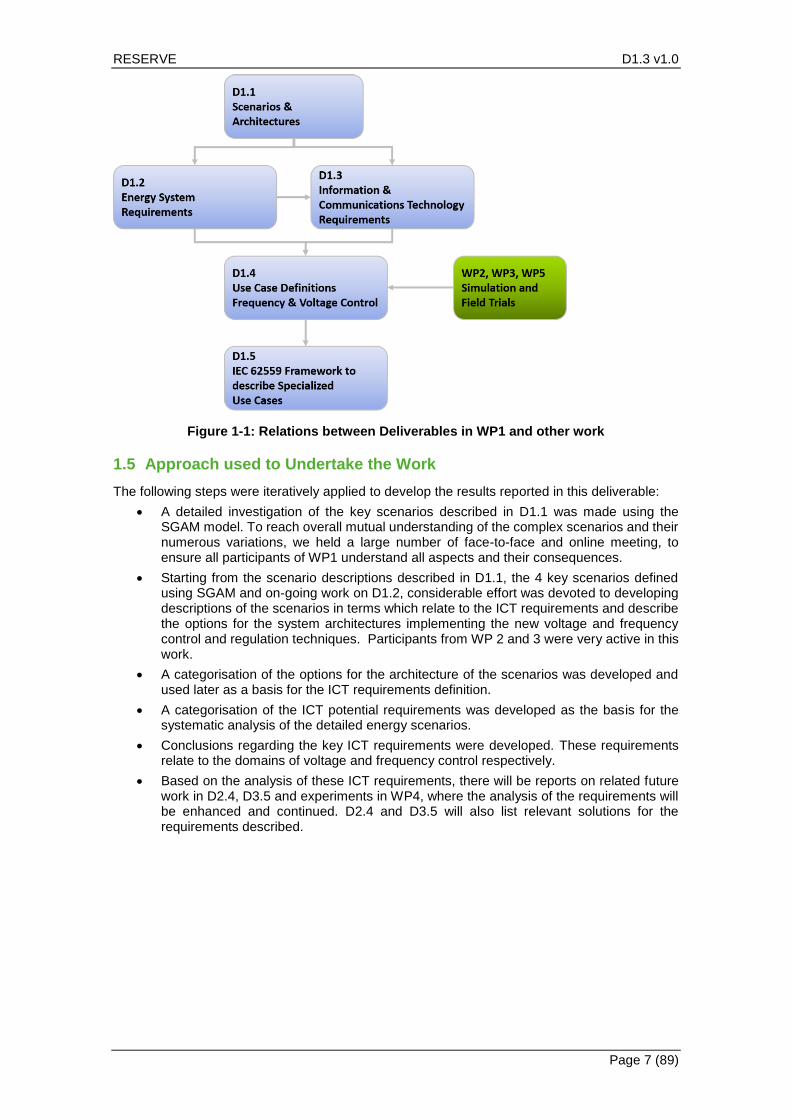
The chart below provides a graphical representation of the dependencies between the deliverables in Work Package 1 of RE-SERVE. The ICT requirements gathered in this document are in turn vital input towards D1.4 Section 2 “High-level use cases assessment”, as there is a need to provide clear definitions for the use case key performance indicators to support the voltage and frequency research concepts development in WP2 and WP3.

RESERVE D1.3 v1.0

(89)

Figure 1-1: Relations between Deliverables in WP1 and other work

1.5 Approach used to Undertake the Work

The following steps were iteratively applied to develop the results reported in this deliverable:

• A detailed investigation of the key scenarios described in D1.1 was made using the SGAM model. To reach overall mutual understanding of the complex scenarios and their numerous variations, we held a large number of face-to-face and online meeting, to ensure all participants of WP1 understand all aspects and their consequences.

• Starting from the scenario descriptions described in D1.1, the 4 key scenarios defined using SGAM and on-going work on D1.2, considerable effort was devoted to developing descriptions of the scenarios in terms which relate to the ICT requirements and describe the options for the system architectures implementing the new voltage and frequency control and regulation techniques. Participants from WP 2 and 3 were very active in this work.

• A categorisation of the options for the architecture of the scenarios was developed and used later as a basis for the ICT requirements definition.

• A categorisation of the ICT potential requirements was developed as the basis for the systematic analysis of the detailed energy scenarios.

• Conclusions regarding the key ICT requirements were developed. These requirements relate to the domains of voltage and frequency control respectively.

• Based on the analysis of these ICT requirements, there will be reports on related future work in D2.4, D3.5 and experiments in WP4, where the analysis of the requirements will be enhanced and continued. D2.4 and D3.5 will also list relevant solutions for the requirements described.

RESERVE D1.3 v1.0

(89)

2. Main Scenarios and their Options

The technical and commercial aspects of power networks are evolving rapidly. New services, new technologies, new stakeholders, and new business models emerge, and the industry will face continuous evolution of these aspects in the coming years.

2.1 Sector Actors in Future Energy Networks

The following paragraphs gives short descriptions of the most prominent sector actors in the Energy Networks for the next ten years.

Transmission System Operator (TSO): a legal actor responsible for operating, maintaining, and developing the transmission system in a country or a certain region of the country. The TSO is responsible for trading power with the neighbour countries.

Distribution System Operator (DSO): a legal actor responsible for operating, maintaining, and developing the distribution systems in a given area, and its connections with other systems. The DSO aims to balance reasonable demand and supply of energy, and thus maintains a stable grid.

Virtual Power Plant (VPP): VPP is a system that integrates several types of power sources, such as wind-turbines, small hydro, photovoltaics, back-up gensets, and batteries, so as to give a reliable overall power supply. The sources are often a cluster of distributed generation systems, and are typically orchestrated by a central authority.

Aggregator: the commercial aggregator (CA) receives forecasts for demand and distributed energy sources (DERs), regarding the load area which it has been assigned to. Forecasts and demand are available at the CA data exchange platform. The CA formulates the offers for flexibility services and energy production/consumption for its load areas, and then sends the offers to the market operator. Consequently, after receiving the schedules for the DERs, once the market clearing and validation phases have been completed, the CA forward the schedules to the corresponding DERs. The Aggregator presented here is in a preliminary form, as it is not yet possible to define it in detail without further assumptions on the operation of the markets.

Prosumer: in the past, the role of energy consumer and energy supplier was clearly separated. With the advent of renewable energy generation, that is no longer the case. An increasing number of private and commercial consumers are also operating photo-voltaic generation equipment, and wind mills whose energy will be inserted into the local smart grid.

Microgrids: they comprise Low-Voltage (LV) distribution systems with distributed energy resources (DERs) (microturbines, fuel cells, PhotoVoltaics (PV), etc.), storage devices (flywheels, batteries) energy storage system and flexible loads. Such systems can be operated in both non-autonomous way (if interconnected to the grid) or in an autonomous way (if disconnected from the main grid).

2.2 Frequency Control Scenarios

The most critical application of grid stabilisation deals with frequency control. This application is performed in different time frames, with different network components and architectures, and with two different approaches labelled Sf_A, Mixed Mechanical-Synthetic Inertia, and Sf_B, Full Synthetic Inertia.

In frequency control, the project will study the impact of having 100% at three different time scales.

2.2.1 Time Scales in Frequency Control

The time limits in the following sections are approximate. The aim is to reduce these time frames in the mid-term future. Frequency control using hydro power for stabilisation, as in scenario Sf_A, is slower, while purely synthetic inertia scenarios as Sf_B will be faster.

Inertial Control

The inertial control aims to provide the virtual inertia, at the instance of disturbance, that contributes to a decreasing rate of change of frequency (RoCoF), to be maintained within the applicable thresholds. Inertial control provides frequency stabilisation in periods of less than 5 seconds, additional layers may be added within RoCoF reducing the time window to much less than 5 seconds, to probably approx. 1 second; this point needs more study in the project. Architectures likely to be used are decentralised and distributed control schemes.

RESERVE D1.3 v1.0

(89)

Primary Control

Primary control is executed in periods of about 5 to 30 seconds, additional layers may be added in primary frequency control reducing the time window available for reaction due to the fast dynamics of the system; this point needs more study in the project. Primary control is based on decentralised or distributed architectures, see below. The dimensioning of the power reserves in the two primary control options is important and is the factor which enables the decision to be made on whether an energy resource is managed using decentralised or using distributed primary control.

Primary control will use the frequency containment reserve in the network.

Secondary Control

Secondary frequency control balances the frequency in periods of over 30 seconds up to 15 minutes. Some countries may have other definitions of secondary control time frames. Common, international time frames will be needed for deployment of technical measures across the European Union. A key factor for improving secondary control is the creation of control loops covering several countries or for regions. Secondary control in different countries is currently organised per country, except for Spain and Portugal which have an organised collaboration for secondary frequency control. Architectures likely to be used to implement secondary control are central control schemes; see section 2.2.2.1 below.

Secondary control will use the frequency restoration reserve in the network.

Consider Figure 2-1: Time scales of frequency control. Frequency fo is the target (nominal) value, such as 50 Hz. When the disturbance sets in, Inertial Response or control is the first counter measure, see red line labelled “RoCoF” in the image. Primary control is the second step which stabilizes system frequency by balancing the power generation and demand. The primary control should ensure that the frequency reaches at least minimum threshold value fss again (green dashed line). The third step, finally, is secondary control which aims to raise/ lower the frequency back to the target value over time in case of under/over frequency problem, respectively.

Figure 2-1: Time scales of frequency control

2.2.2 Control Architectures in Frequency Control

Centralised Architecture in Frequency Control

Centralised control of all RES sources is needed to create awareness of the status of frequency in the system as a whole but has the drawback that it operates in a slower timeframe as it requires communication to a central control centre which computes frequency and returns commands for control. In large networks, communications latency is the main latency factor. Communications links need to be installed between all RES sources and the control centre of the local DSO, which is in turn connected to the control centre of the TSO.

In Figure 2-2: Centralised Control in Frequency Stabilisation, the data analysis, the stabilisation algorithms, and the command delivery are carried out by the EMS on TSO level, and the DMS on DSO level, respectively.

RESERVE D1.3 v1.0

(89)

Figure 2-2: Centralised Control in Frequency Stabilisation

These control centres represent a security risk as a failure of a control centre will cause a range of disturbances, such as cascading failures resulting in black-outs, in the power networks.

In a centralised control centre, the algorithm of the frequency divider needs to be computed very fast, how fast depends on the size of the system. Computation close to real-time speed is required. The frequency at all points in the network is computed and then decisions can be made on changes to make in the network and the appropriate signals are communicated to the individual RES sources in the network. For a scenario in which synchronous generation is available, the algorithm will use either the information on the rotor speed of the synchronous machines or use the PMU measurements from the system.

For the scenario of 100% RES without synchronous generation, this algorithm needs to be improved. It could potentially use the PMU measurements or the connected virtual synchronous machines.

Decentralised Architecture in Frequency Control

A further option for top-down frequency control could be to apply the frequency divider algorithm in neighbouring regions rather than for a whole network at once. Less information is available but the local control has an improved quality as it is based on the average values for the neighbouring regions and offers a good compromise between centralised and distributed control.

For example, decentralised primary control is independent and automatic, which means decentralised control. Mixed signals, consisting of both RoCoF and the amount of the change of frequency, abbreviated as Δf, can be used in primary control level to allow faster reserve deployment with implicit inertial response. However, this will require a classification of the energy resources in terms of their technical capabilities.

Controlling the frequency will not require any communications in this architecture. However, for security purposes, each RES, each storage device, every prosumer or each DC grid controller may be connected to the central control room of the TSO/DSO in order to monitor the correct operation of the systems to ensure reliability. Smart meters could play the role of interface to the inverters of the loads or prosumers. The smart meters are already interfaced with communications to the DSOs.

The following figure explains the difference between decentralised and distributed control architecture and the communication paths, the latter being discussed in the next chapter. The picture is simplified, but should just highlight the two concepts.

RESERVE D1.3 v1.0

(89)

Figure 2-3: Comparison of Decentralised and Distributed Architectures

Consider the following Figure 2-4: Extended example of future Frequency Control in a Decentralised Architecture below. It shows a logical overview of the communications structure in a decentralised approach to frequency control on DSO level.

Figure 2-4: Extended example of future Frequency Control in a Decentralised Architecture

The frequency control is carried out independently between the different DSOs, without direct intervention of the TSO. The TSO is only providing rules, distributes alerts, and receives alerts and statistics from its distribution partners. The various DSO do not interact with each other, they can stabilize the frequency themselves. In the medium voltage (MV) network, virtual power plants (VPP) and individual power plants may balance their frequency directly, if they have direct access to energy storage systems, to inject or absorb power to or from their system.

In the low voltage (LV) or feeder network, microgrids and some local inverters may also control their own frequency, if they have immediate access to their local energy storage systems.

The decentralised architecture is mainly used for fast response to frequency variations, i.e. in inertial control and in primary control, see chapter 2.2.1 Time Scales in Frequency Control above.

Distributed Architecture in Frequency Control

In a distributed control strategy, the actions of the local controllers are coordinated.

RESERVE D1.3 v1.0

(89)

In inertial control, for instance, a reaction to RoCoF signals would establish the need for a common signal. This is because RoCoF is not the same all over the power system. Since the biggest problems in terms of RoCoF are created in the case of short-circuits near the generator followed by loss of generation, the highest RoCoF will be observed at the location of the short-circuit; then, the longer the distance from the short-circuit location, the smaller the RoCoF will be. For this reason, the fastest and biggest intervention will be from the sources closest to the short-circuit location.

In order to have identical responses with the same RoCoF signal, there is need for coordination.

Depending on the control scheme, different communications links will be required. The geographical distances to be covered will depend on the scale of the system using the distributed control strategy, which could be applied at TSO level or down to micro-gird levels. The number of devices (converters of RES, battery storage, prosumers, and micro-grids) which need to be connected to DSO and TSO control centres is also variable and will influence the choice of communications channel. The relevant latency will depend on the use of the network architecture for either RoCoF or primary control. The distributed architecture is not likely to be used for secondary control.

2.2.3 Two frequency control scenarios in RESERVE: Sf_A and Sf_B

This project investigates two different frequency control scenarios which are compared in the following sections.

Sf_A – Mixed Mechanical-Synthetic Inertia

For 100% RES, this scenario combines the use of mechanical inertia from hydro and geothermal power units with renewable energy sources such as photovoltaics and wind turbines. Therefore, the focus of this scenario is on high and medium voltage networks. PV and wind turbines require synthetic inertia to balance the frequency in the network.

In addition, the scenario will include the investigation of demand-side control aspects, where the DSO is able to stabilize the grid by controlling the energy balance of the load (consumers) and prosumers in the network. This approach is suitable for smaller grids.

See chapter 8.1.1 Detailed Analysis of the Sf_A Scenario in the Appendix, for a detailed analysis of the business and data aspects of this frequency control concept.

Sf_B – Synthetic Inertia

This scenario will focus on energy production with 100% provided by non-hydro renewable energy sources, i.e. photovoltaics and wind turbines. Hence, there is no mechanical inertia in the energy production. Instead, synthetic inertia is provided by the stored energy in the rotating masses of wind turbines and storage systems. Due to the very high deployment of offshore wind farms in Europe, High Voltage Direct Current (HVDC) grids will be integrated into the AC networks to deliver and share the bulk power generated from the offshore wind farms. Also, the HVDC grids will play a significant role in exchanging the power between national and international areas for balancing energy and frequency stabilization purposes.

Due to the fully converter-interfaced system generation, the very fast system dynamics will result in a reduced time window for the frequency control categories (inertial, primary, secondary), and additional control layers will be most likely integrated into the existing frequency control categories.

Also, the concept of Linear Swing Dynamics (LSD) will be developed in the control of RES converters, not the storages. This will result in a linear dynamical system and provide significant features in system stability analysis, frequency regulation and control. However, the applicability of LSD in a system with limited mechanical inertia, i.e. scenario SF_A, is still to be studied by the project.

Comparison between Sf_A and Sf_B

The main differences between SF_A and SF_B scenarios are provided in the following table.

RESERVE D1.3 v1.0

(89)

Table 2-1: Comparison between Scenarios Sf_A and Sf_B

Aspects

Frequency Control Scenario

Sf_A Sf_B

System Generation

Mix of Hydro, geothermal, wind and PV power plants

Wind and PV power plants

System inertia Mixed mechanical and synthetic

(virtual) inertia Fully synthetic (virtual) inertia

Inclusion of DC technology

Fully AC network Hybrid AC/DC network

System dynamics Slower dynamics due to the

mechanical dynamics from existing synchronous generation

Very fast dynamics due to the fully converter-connected network

generation

Applicability of Linear-Swing

Dynamics (LSD)

Probably not applicable

(to be studied for a limited mechanical inertia systems)

Applicable for all the RES-interfaced converters

Control time window

Same as today’s (ENTSO-E) time frames

Reduced time window, and probably additonnal control layers will be

inclded

It can be observed from the table that the main differences between Sf_A and Sf_B are in terms of system generation, inertia, dynamics and control time window. In addition, a very fast and reliable communication is more critical in Sf_B than in Sf_A.

It is worth mentioning that there is no difference in the control architecture between Sf_A and Sf_B. In other words, both scenarios could have: decentralised and distributed control for inertial and primary control, and centralised for secondary control. More details about frequency control architecture is provided in Subsection 3.1.

2.3 Voltage Control Scenarios

In the evolution towards 100% RES, the objective of voltage control is to balance the voltage in future low voltage distribution grids connecting local loads and prosumers as well as energy storage facilities. The aim is to stabilize the voltage as local as possible, so that decisions and control commands can be issued as quickly as possible. Consumers and prosumers should not experience any disturbances of their power supply.

In these scenarios, energy generation relies on renewable sources supplying direct current (DC), hence the role of the inverter converting DC to AC power, as the crucial element in these scenarios. The inverters will measure the voltage (V), current (I) and active and re-active powers (P and Q). The inverters may also change the amount of power injected into the grid, and connect and disconnect end-points from the LV network. Therefore, the communication flow from the regional control centre of the DSO terminates at the inverter.

If commercial aggregators exist in the LV grid, then they will provide data collection and analysis services for the DSO, combining the output of all end-points in the area for which the aggregator provides such services.

Consider the image below, Figure 2-5: Decentralised Architecture for Voltage Control. It shows the logical overview of a distribution grid, where the regional control is performed by the secondary substation automation unit (S. SAU), communicating with the inverters. The inverters monitor and

RESERVE D1.3 v1.0

(89)

control the state of the connected loads, small-scale batteries, heat pumps, EV charging stations, PV systems, and wind turbines. In addition, the picture includes microgrids as well as commercial aggregators. While microgrids may perform independent voltage control for their subnetworks including end-points for consumers, prosumers and small-scale storage units (batteries), the commercial aggregator does not normally provide such service, but will aggregate and analyse the data for the DSO.

Figure 2-5: Decentralised Architecture for Voltage Control

On European level, there are ongoing discussions, to extend the role of the Aggregator from a commercial to a much more technical focus. In this case, the Aggregator would provide voltage management for this part of the distribution network, too. The following image shows this situation.

Figure 2-6: Decentralised Voltage Control with Technical Aggregator

The control architecture in this picture is de-centralised, as different regional subnetworks do not communicate with each other. This means that one S. SAU does not receive or process the data from a neighbouring S. SAU.

2.3.1 Use Case Voltage Control Sv_A: Dynamic Voltage Stability Monitoring

The dynamic voltage stability monitoring (DVSM) is a decentralised approach for monitoring transient voltage stability in LV distribution grids. The secondary substation automation unit (SSAU) hosts the voltage stability algorithm as a software component, and this program behaves as a coordinator gathering the information from the inverters to compute stability margins and

RESERVE D1.3 v1.0

(89)

send back control commands back to the inverters. The SSAU performs the evaluation of stability margins once an hour for each inverter.

The approach in Sv_A is based on the Middlebrook theory where the stability can be determined using the inverter output impedance and the grid impedance as input. For the measurement of the impedances, a wide-band system identification (WSI) tool is present in the inverter. The WSI tool injects a pseudo-random binary sequence (PRBS) signal into the controller in the inverters and processes the incoming voltage and current measurements to determine the impedance. Consider an inverter A, and an inverter B which neighbours inverter A. The SSAU sends an initiation signal to the inverter A to use its WSI tool to measure the grid impedance. An inverter cannot measure its own impedance. For this reason, the SSAU sends a command to inverter B to apply its WSI tool to inject a PRBS signal to measure the output impedance, the SSAU instructs inverter A to record current and voltage measurements. The WSI tool of inverter A can then compute the output impedance of inverter A. This process is explained in more detail in chapter 8.2.1.1 in the Appendix.

The coefficients of the identified grid and output impedance are sent back to the SSAU. The SSAU performs stability analysis based on the Middlebrook theory, computes the stability margins and if required, sends back control commands to the virtual output impedance controller (VOI) of the inverter A. This process is repeated for Inverter B and furthermore for all other inverters present under the direct control of the SSAU.

2.3.2 Use Case Voltage Control: Sv_B, Active Voltage Management

The Active Voltage Management (AVM) technique reduces the voltage control problem to a local objective for each RES unit: to continuously target a single voltage value by maintaining a relationship between the reactive power provided and the voltage observed. This style of control is known as a volt-VAr curve. The target voltage is obtained using an AC optimal power flow (OPF) centralised approach that is capable of multi-period analysis. Any objective that can be formulated within the realm of AC OPF analysis can be investigated, producing an objective-governed volt-VAr curve.

These curves constrain the operation of the units based solely on their available reactive power capability and the present voltage measurement to fulfil the objective that realising the target voltage will bring about. In D3.2, a case study is presented showcasing the stages involved in an offline-modelling technique, to produce these volt-VAr curves.

The consequence of this is that in an online deployment setting, the voltage control problem is reduced to a linear relationship between the target voltage of the RES unit and the reactive power output of the unit. This provides the means to operate in a decentralised manner where the complexity of AC power flow solutions need not be calculated on a continuous basis.

Reducing the offline centralised analysis to an online and decentral deployment through the means of optimally chosen volt-VAr curves, gives a practical means to facilitate the objectives of the DSO. These objectives could, in future, be in response to market mechanisms, or simply regulate the network in the most efficient way possible. This capability is increasingly important considering that future voltage management concepts should provide the means to making best use of the finite capacity of distribution networks.

For details on the implementation and the SGAM business and data models, please see this

section below in the appendix: chapter 8.2.3 SGAM for the Sv_B Scenario.

2.3.3 Comparison of Scenarios Sv_A and Sv_B

Sv_A: Dynamic voltage stability monitoring

• Addresses dynamic voltage stability or transient voltage stability, where the time frame is of the order of milliseconds.

• Requires a WSI tool, VOI controller and communication ports in the inverter.

• Requires SSAU to have the system level voltage stability algorithm.

• The SSAU and the inverters communicate through mobile networks, such as LTE or 5G.

• Works on an hourly basis to monitor system level stability, when stability of the system is endangered, corrective actions are undertaken to ensure sufficient stability margins.

RESERVE D1.3 v1.0

(89)

• No need to compute optimal power flow set-points, i.e. reference power values for the inverter.

• Does not manage voltage in steady state, i.e. in larger time frames.

Sv_B: Active voltage management

• Addresses optimal power flow for a 100% RES network and manages voltage actively, and uses the service of household inverters. The time frame is of the order of minutes.

• Requires communication ports in the inverter.

• Requires the addition of the volt-VAr curve functionality in SSAU.

• The SSAU and the inverters communicate through mobile networks, such as LTE or 5G.

• Works every 5 minutes, with its objective to maintain voltage within stipulated limits as per grid codes by solving an optimisation problem to minimise objectives such as losses.

• Does not compute dynamic stability margins.

• Note that Sv_A and Sv_B can co-exist in future networks.

• Sv_B does not perform corrective action when stability margins are low.

2.4 Overview

The following matrix compiles the combinations of the frequency control scenarios and their key parameters in this project.

Figure 2-7: Overview of scenarios for Frequency Control

The following matrix compiles the combinations of the voltage control scenarios and their key parameters in this project.

RESERVE D1.3 v1.0

(89)

Figure 2-8: Overview of Scenarios for Voltage Control

RESERVE D1.3 v1.0

(89)

3. Scenarios and ICT Requirements

This chapter describes the scenarios so that the resulting ICT requirements can be presented in more detail. In frequency control, each scenario has various alternatives, which are listed and described as well.

3.1 Frequency Control Scenarios

As explained in Subsection 2.2, there is no difference in the control architecture between Sf_A and Sf_B. To avoid repeating graphs in multiple sections, the following frequency control graphs are valid for both Sf_A and Sf_B, with the consideration of two main differences in the latter:

1- Elimination of hydro power plants in Sf_B

2- Inclusion of DC grid converters in Sf_B

Hence, the following graphs illustrating the frequency control architecture for both scenarios, with the following differences:

Different types of power generation systems, use of mechanical and synthetic inertia, different dynamics, and shorter control time window for Sf_B. In addition, a very fast and reliable communication is more critical in Sf_B than in Sf_A.

3.1.1 Inertial Control

TSO, Decentralised Control, Sf_A

1) Summary of Scenario Aspects

• The goal of the inertial control is to respond very fast in order to prevent any short-term frequency changes in case of sudden power unbalance.

• The decentralised control is established by the independent contribution of all power generation sources having installed power greater than a predefined value, and which are connected to the power grid. Since no external communication is required, this type of control is highly robust. Concepts such as virtual power plants or microgrids are not used in this type of control.

Figure 3-1: Decentralised Inertial Control at TSO-level

RESERVE D1.3 v1.0

(89)

2) Communications Architecture

• No communication infrastructure with external units is necessary at this level. All measurements, data acquisition and processing, decision and control are performed locally by means of metering units, RTU and PLC. The effective control is done either at the inverter level or the turbine, depending on the type of the generation sources.

• A generic representation of the decentralised inertial control in the TSO network is shown in Figure 3-1: Decentralised Inertial Control above.

3) Functional Requirements

• Frequency and RoCoF values measured locally are the inputs for this level of control.

• There are two types of controlled generation units: i. Turbine driven synchronous generator (in the case of hydraulic power plants); ii. Power electronic-based converter energy systems (e.g. PV systems, wind systems or storage systems).

i. The input signals are processed by the speed governor, which triggers the change in the water flow admission to the turbine.

ii. The input signals are processed by the controller of the electronic-based converter that in turn will change the voltage and/or current output in such a way to change the active power output.

4) Performance Requirements

• For inertial control, the solution benefits from the most minimum transmission and computation times, that is in the range of below 1 second. In this scenario, the actual latency and jitter effects depend only on the technology used at the local level.

• Data Volume/Bandwidth: In the future, as the RoCoF will be used, large amount of data will be processed. For this purpose, new computational equipment might be necessary. Estimated data volume is 100 MByte for one hour of measurements.

5) Security Requirements

• No special security requirements are considered necessary, because all local systems and operating in closed loop.

TSO, Decentralised Control, Sf_B



• There is one type of controlled generation units, i.e. converter-interfaced energy systems (e.g. PV plant, wind power plant, or storage systems).

• The decentralised control is established by the independent contribution of wind power plants, storage-connected PV plants, and individually connected storage systems.

• Since no external communication is required, this type of control is highly robust. Concepts such as virtual power plants or microgrids are not used in this type of control.



• A generic representation of the decentralised inertial control in the TSO network is shown in Figure 3-1: Decentralised Inertial Control above.


RESERVE D1.3 v1.0

(89)


• The input signals are processed by the converter’s controller, that in turn will change the voltage and/or current output in such a way to change the active power output.


• The actual latency and jitter effects the control performance.

• Data Volume/Bandwidth: In the future, as the RoCoF will be used, large amount of data will be processed. For this purpose, new computational equipment might be necessary.


• No special security requirements are considered necessary, because all local controlled units are operating in closed loop.

TSO, Distributed Control, Sf_A


• Tens up to hundreds of end-points including generation and storage entities located in transmission networks could be integrated in such a control scheme, see Figure 3-2: Distributed Inertial Control at TSO-level.

• A RoCoF unit that integrates frequency estimation and RoCoF calculation, installed in the transmission network substation, sends control signals to all these end-points.

• In today’s networks, this type of control was not necessary, because the existing power plants have sufficient mechanical inertia to limit the frequency dips.

• Activities in one Cycle of RoCoF Control

Step 1. The RoCoF unit detects dangerous situation based on measurements.

Step 2. The RoCoF unit calculates the necessary power to be changed.

Step 3. The RoCoF unit sends individual control signals to each end-point. Tens up to hundreds of signals need to be sent.

Step 4. The end-points receive the control signal from the RoCoF unit and apply changes at the inverter, eg. for PV plants, wind turbines, and storage systems, or at the speed governor for hydraulic plants to adapt the level of power generated.

Step 5. For monitoring purposes, the end-points send an acknowledgement to the RoCoF unit that the power level has been changed.

RESERVE D1.3 v1.0

(89)

Figure 3-2: Distributed Inertial Control at TSO-level


• The communication architecture is illustrated in Figure 3-2: Distributed Inertial Control at TSO-level. The optical ground wire (OPGW) installed on the transmission lines can be used for communication between the RoCoF unit and the end-points. Alternatively, 5G mobile radio is highly suitable for linking the generation units and the control unit.

• Technology: either fibre-optics or 5G mobile radio, depending on commercial aspects for linking the end-points with the RoCoF control unit.

• The RoCoF unit can be a component of the substation automation (SSAU).


• The individual controllers for the end-points are located in the inverters, which need to be equipped with additional communication ports. The external signals are integrated into the control pattern of the inverter. At the TSO level, the end-points incorporate RTUs, and thus the control signal is not directly sent to the inverter.

• As the inertial control requires a reaction in terms of power control within 1-5 seconds from the instant of detection of the RoCoF variation, extremely fast communication is required, contributing to the use case for 5G mobile radio.

• The information, in form of control signals, is unidirectional, from the RoCoF unit to the end-points.

• The RoCoF unit calculates the RoCoF in an optimum point, performs calculations for power change, and sends control signals to the end-points. The RoCoF is continuously calculated, with a sample rate of 10 milliseconds. The control signals are sent only when necessary, i.e. when the RoCoF exceeds certain limits. When necessary, the control signal should reach the controlled components within a timeframe well below one second.


RESERVE D1.3 v1.0

(89)

• Latency: as the functional requirements indicate above, extremely short latencies help to provide the best possible inertial control in the grid. One complete cycle including measurements, data analysis and control response should be executed in less than one second.

• Jitter can alter the quality of the control if the control signal is delayed by more than 1 second. If the performances of the telecommunication systems in the future cannot reduce the jitter to acceptable values, then increasing the number of the RoCoF units and reducing the number of controlled components attached to it might be a solution.

• Data Volume/Bandwidth: all exchanged information consists of a few Kbytes of data. The exchange rate can be 0.5 seconds. Locally, the RoCoF unit can be required to process large amounts of data.


• Authentication: all parties in the communication should use the latest authentication processes according to the latest security standards defined by IEEE, IEC and other prominent standardisation bodies. Authentication techniques can be leveraged from future 3GPP (5G) mobile communication standards such as Generic Bootstrapping Architecture (GBA).

• Secure end-to-end data encryption is required on all links, if the communication does not use a closed loop, or private network. For instance, using 5G mobile connections, encryption of measurements and commands is recommended.

• Data integrity is important and needs to ensure that any measurements and control information sent from one point to another in the network is not changed by malicious parties. This is an essential requirement imposed on communication infrastructure. Standards such as IEC 61907 can be investigated for different control scenarios.

TSO, Distributed Control, Sf_B


• Tens up to hundreds of end-points including generation and storage entities located in transmission networks could be integrated in such a control scheme, see Figure 3-2: Distributed Inertial Control at TSO-level.

• The inertial control, also called RoCoF unit, integrates frequency estimation and RoCoF calculation, installed in the transmission network substation, and sends the control signals to all these end-points.

• In today’s networks, this type of control is not necessary, because the existing power plants have sufficient mechanical inertia to limit any potential frequency dips.

• Activities in one Cycle of inertial Control

Step 1. The inertial control detects dangerous situation based on measurements.

Step 2. Calculate the necessary power to be changed.

Step 3. Sends individual control signals to each end-point. Tens up to hundreds signals need to be sent.

Step 4. The end-points receive the control signal from the inertial control and apply changes at the inverter, e.g. for PV plants, wind turbines, and storage systems, to adapt the level of power generated.

Step 5. For monitoring purposes, the end-points send an acknowledgement to the inertial control that their power level has been changed.


• This control has the criticality in time and system security, as it should be executed in a very fast manner, approx. within 1-2 seconds. In addition, this control relies on communication due to the coordinated activities among the distributed inertial controllers. Hence, a very fast, robust and reliable communication technology/architecture should be used.

RESERVE D1.3 v1.0

(89)

• The communication architecture is illustrated in Figure 3.2. The optical ground wire (OPGW) installed on the transmission lines can be used for communication between the inertial control and the end-points. Alternatively, 5G mobile radio is highly suitable for linking the generation units and the control unit.

• In case of terrains, the fibre-optic might be costly, and hence, another communication technology could be used in such areas.

• Technology: either fibre-optics or 5G mobile radio, depending on the geographical area, distances and other commercial aspects.

• The inertial control can be coordinated with the substation automation (SSAU).




• The information, in form of control signals, is unidirectional, from the inertial control to the end-points.

• The inertial control calculates the RoCoF in an optimum point, performs calculations for power change, and sends control signals to the end-points. The RoCoF is continuously calculated, with a sample rate of 10 milliseconds. The control signals are sent only when necessary, i.e. when the RoCoF exceeds certain limits. When necessary, the control signal should reach the controlled components within a timeframe well below one second.


• Latency: as the functional requirements indicate above, extremely short latencies help to provide the best possible inertial control in the grid. One complete cycle including measurements, data analysis and control response should be executed in very less than one second.

• Jitter can alter the quality of the frequency control if the control signal is delayed by more than 1 second.

• Data Volume/Bandwidth: all exchanged information consists of a few Kbytes of data. The exchange rate can be less than 0.5 seconds.





DSO, Decentralised Control, Sf_A


• The goal of the inertial control is to respond very fast to prevent any short-term frequency changes in case of sudden power unbalance.

• The decentralised control is established by the independent contribution of all power generation sources having installed power greater than a predefined

RESERVE D1.3 v1.0

(89)

value, and which are connected to the power grid. Since no external communication is required, this type of control is highly robust. Concepts such as virtual power plants or microgrids are not used in this type of control.

Figure 3-3: Decentralised Inertial Control at DSO-level



• A generic representation of the decentralised inertial control in the DSO network is shown in Figure 3-3: Decentralised Inertial Control at DSO-level above.







• For inertial control, the solution benefits from the most minimum transmission and computation times, i.e. in the range of below 1 second. In this scenario, the actual latency and jitter effects depend only on the technology used at the local level.

• Data Volume/Bandwidth: In the future, as the RoCoF will be used, large amount of data will be processed. For this purpose, new computational equipment might

RESERVE D1.3 v1.0

(89)

be necessary. Estimated data volume is 100 MByte for one hour of measurements.


No special security requirements are considered necessary, because all local systems and operating in closed loop.

DSO, Decentralised Control, Sf_B



• There is just one type of controlled generation units, i.e. converter-interfaced energy systems (e.g. PV plant, wind turbine, or storage systems).

• The decentralised control is established by the independent contribution of wind power plants, storage-connected PV plants, and individually connected storage systems.

• Since no external communication is required, this type of control is highly robust. Concepts such as virtual power plants or microgrids are not used in this type of control.


• No communication infrastructure with external units is necessary at this level. All measurements, data acquisition and processing, decision and control are performed locally by means of metering units, RTU and PLC (or SSAU). The effective control is done either at the converter level.

• A generic representation of the decentralised inertial control in the DSO network is shown in Figure 3.3



• The input signals are processed by the converter’s controller that in turn will change the voltage and/or current output in such a way to change the active power output.


• The actual latency and jitter directly, determine the control performance. In other words, the better the latency, the faster the stabilisation of the frequency in the grid.

• Data Volume/Bandwidth: In the future, as the RoCoF will be used, large amounts of data will be processed. For this purpose, new computational equipment might be necessary.

• Estimated data volume is 100 MByte for one hour of measurements.


• No special security requirements are considered necessary, because all local controlled units are operating in closed loop.

DSO, Distributed Control, Sf_A

On DSO-level, with distributed control, there are many more, and smaller end-points than on TSO-level.


• Hundreds up to thousands of end-points including flexible loads, prosumers, and storage systems are located in both LV and MV distribution networks will be integrated in frequency control procedures. See Figure 3-4: Distributed Inertial Control at DSO-level.

• A RoCoF unit that integrates frequency estimation and RoCoF calculation will be installed in the distribution network, sending control signals to all these end-points.

RESERVE D1.3 v1.0

(89)

• The RoCoF unit could be implemented on the same platform as the SSAU of the DSO, and there would be no interaction with the EMS of the TSO. Tens of RoCoF units can be implemented in different distribution networks.

• Today, this type of control does not exist today for two reasons: the conventional power plants with mechanical inertia can already provide the necessary frequency control, and no physical infrastructure is available for such scale of communication.

Figure 3-4: Distributed Inertial Control at DSO-level

RESERVE D1.3 v1.0

(89)


• The communication architecture is illustrated in Figure 3-4: Distributed Inertial Control at DSO-level above. There is direct communication between a RoCoF unit and its end-points, and 5G mobile networks are most suitable for this interaction.




• The information, in form of control signals, is unidirectional, from the RoCoF unit to the end-points.

• The RoCoF unit calculates the RoCoF in an optimum point, performs calculations for power change, and sends control signals to the end-points. The RoCoF is continuously calculated, with a sample rate of 10 milliseconds. The control signals are sent only when necessary, i.e. when the RoCoF exceeds certain limits. When necessary, the control signal should reach the controlled components within a timeframe well below one second.









DSO, Distributed Control, Sf_B

On DSO-level, with distributed control, there are many more, and smaller end-points than on TSO-level.


• Hundreds up to thousands of end-points including flexible loads, prosumers, and storage systems are located in both LV and MV distribution networks will be

RESERVE D1.3 v1.0

(89)

integrated in frequency control procedures. Please consider Figure 3-5: Distributed Inertial Control at DSO-level (Sf_B) below.

• An inertial control that integrates frequency estimation and RoCoF calculation will be installed in the distribution network, sending control signals to all these end-points.

• The inertial control could be implemented on the same platform as the SSAU of the DSO. Tens of inertial controllers can be implemented in different distribution networks.

• Additional physical infrastructure will be developed for such scale of communication.

Figure 3-5: Distributed Inertial Control at DSO-level (Sf_B)

RESERVE D1.3 v1.0

(89)


• The communication architecture is illustrated in Figure 3-5. The most relevant communication links the inertial control and its end-points, and 5G mobile networks are most suitable for this interaction. Also, there will be a coordination links among the installed inertial controllers.


• The individual controllers for the end-points are located in the converter, which need to be equipped with additional communication ports. The external signals are integrated into the control pattern of the converter.


• The information, in form of control signals, is unidirectional, from the inertial control to the end-points.

• The RoCoF unit calculates the RoCoF at an optimum point, performs calculations for power change, and sends control signals to the end-points. The RoCoF is continuously calculated, with a sample rate of 10 milliseconds. The control signals are sent only when necessary, i.e. when the RoCoF exceeds certain limits. In this point, the control signal should reach the controlled components within a timeframe well below one second.



• Jitter can alter the quality of the control if the control signal is delayed by more than 1 second.






3.1.2 Primary Control

TSO, Decentralised Control, Sf_A


• The goal of primary frequency control is to stabilize the frequency in case of a large perturbation. For this reason, the primary reserve must be deployed very fast (in less than 30 seconds). The amount of power reserve available for primary control depends on the TSO power system, it is a proportional share of the total power provided in the entire synchronously interconnected power system. In continental Europe, the ENTSO-E will regulate such reserves.

• The decentralised control consists of the independent contribution of all generation sources of installed power greater than a predefined value connected

RESERVE D1.3 v1.0

(89)

to the power grid. Since no external communication is required, this type of control is comparatively robust. Concepts such as virtual power plants or microgrids are not used in this type of control.

• It is not expected that this type of control will change in the future. However, as suggested in our project, we expect that a mixed signal consisting of the RoCoF and frequency variation will be used in the decentralised control.


• No communication infrastructure with external units is necessary at this level. All measurement, data acquisition and processing, decision and control are performed locally by means of metering units, RTU and PLC. The effective control is done either at the inverter level or the turbine, depending on the type of the generation sources.

• See also Figure 3-6: Primary Frequency Control .







• Latency: as the functional requirements indicate above, extremely short latencies help to provide the best possible primary control in the grid. One complete cycle including measurements, data analysis and control response should be executed in less than one second.





RESERVE D1.3 v1.0

(89)

Figure 3-6: Primary Frequency Control at TSO-level

TSO, Decentralised Control, Sf_B


• The goal of primary frequency control is to stabilize the frequency in case of a small-large perturbation. For this reason, the primary reserve must be deployed very fast (in less than 10 seconds). The amount of power reserve available for primary control depends on the TSO power system, it is a proportional share of the total power provided in the entire synchronously interconnected power system. In continental Europe, the ENTSO-E will regulate such reserves.

• The decentralised control consists of the independent contribution of all generation sources of installed power greater than a predefined value connected to the power grid. Since no external communication is required, this type of control is comparatively robust. Concepts such as virtual power plants or microgrids are not used in this type of control.



• No communication infrastructure with external units is necessary at this level. All measurement, data acquisition and processing, decision and control are performed locally by means of metering units, RTU and PLC. The effective control is done either at the converter level.

• See also Figure 3-5: Distributed Inertial Control at DSO-level (Sf_B) above.


• Frequency and RoCoF values are measured locally, and they are the inputs for this level of control.

• There is one type of controlled generation units, i.e. converter-interfaced energy systems (e.g. PV plant, wind power plant, or storage systems).

i. The input signals are processed by the converter’s controller that in turn will change the voltage and/or current output in such a way to change the active power output.

RESERVE D1.3 v1.0

(89)


• Latency: as the functional requirements indicate above, extremely short latencies help to provide the best possible control in the grid. One complete cycle including measurements, data analysis and control response should be executed in less than one second.




• No special security requirements are considered necessary, because all local systems (controlled units) are operating in closed loop.

TSO, Distributed Control, Sf_A

In scenario Sf_A, large power plants are directly connected to the transmission grid. Therefore, the frequency will be controlled by the TSO, and not by each energy generator individually.

TSO, Distributed Control, Sf_B


• Large PV and wind power plants are connected to the transmission network. Their primary control will be coordinated to provide the primary power reserve in case of perturbation (power disturbance).

• An example of this concept is the inclusion of HVDC grids. Considering a power system composed of several non-synchronous AC areas (networks) connected by a multi-terminal HVDC grid as shown in Figure 3-7: Distributed primary frequency control in HVDC-connected AC networks. In this context, a distributed primary frequency control will modify the power injections from the diff erent AC areas into the DC grid so as to make the system collectively react to load (power) imbalances. This collective reaction allows each individual AC area to downscale its primary reserves.

Figure 3-7: Distributed primary frequency control in HVDC-connected AC networks


• The controllers of the converters communicate directly with each other. The links can be implemented with fibre-optic cables due to the long distances between the controllers. In case of difficult terrains, however, safely placing cables underground is too costly, and different communication technologies should be used.


• The converters’ controllers need to be provided with additional communication port. The external signal is integrated into the control diagram of the converter.

• As the primary control requires deployment of the power reserve within few seconds, the entire chain of measurement, data collection, data processing and communication should be done in a very fast manner accordingly.


• Latency: as the functional requirements indicate above, extremely short latencies help to provide the best possible control consistence in the grid. One complete

RESERVE D1.3 v1.0

(89)

cycle including measurements, data analysis and control response should be executed in very less than one second.


• Data Volume/Bandwidth: all exchanged information consists of a few Kbytes of data. The exchange rate can be very less than 0.5 seconds.





DSO, Decentralised Control, Sf_A


• The goal of primary frequency control is to stabilize the frequency in case of a large perturbation. For this reason, the primary reserve must be deployed very fast (in less than 30 seconds). The amount of power reserve available for primary control depends on the DSO power system, it is a proportional share of the total power provided in the entire synchronously interconnected power system. In continental Europe, the ENTSO-E will regulate such reserves via the TSOs.




• No communication infrastructure with external units is necessary at this level. All measurement, data acquisition and processing, decision and control are performed locally by means of metering units, RTU and PLC. The effective control is done either at the inverter level or the turbine, depending on the type of the generation sources.

• See also Figure 3-8: Decentralised Primary Frequency control.







RESERVE D1.3 v1.0

(89)






Figure 3-8: Decentralised Primary Frequency control at DSO-level

DSO, Decentralised Control, Sf_B


• The goal of primary frequency control is to stabilize the frequency in case of a large perturbation. For this reason, the primary reserve must be deployed very fast (in less than 10 seconds). The amount of power reserve available for primary control depends on the DSO power system, it is a proportional share of the total power provided in the entire synchronously interconnected power system.

• The prosumers and microgrids will contribute with frequency stabilization.


RESERVE D1.3 v1.0

(89)

• As suggested in our project, we expect that a mixed signal consisting of the RoCoF and frequency variation will be used in the decentralised control.


• No communication infrastructure with external units is necessary at this level. All measurement, data acquisition and processing, decision and control are performed locally by means of metering units, RTU and PLC. The effective control is done at the converter level.

• See also Figure 3-8: Decentralised Primary Frequency control at DSO-level.



• There is one type of controlled generation units, i.e. converter-interfaced energy systems such as PV plants, wind turbines, and storage systems.

i. The input signals are processed by the controller of the electronic-based converter that in turn will change the voltage and/or current output in such a way to change the active power output.


• Latency: as the functional requirements indicate above, extremely short latencies help to provide the best possible control in the grid. One complete cycle including measurements, data analysis and control response should be executed in very less than one second.

• Jitter can alter the quality of the control if the control signal is delayed by one second.



• No special security requirements are considered necessary, because all local systems (controlled units) are operating in closed loop.

DSO, Distributed Control, Sf_A


• On DSO-level, there are up to thousands of individual end-points including flexible loads, prosumers, and storage systems. The end-points are located in LV and MV distribution networks that will participate in frequency control mechanisms. See Figure 3-9: Distributed Primary Frequency control below.

• A RoCoF unit, which integrates frequency estimation and RoCoF calculation, is installed in the distribution network and sends control signals to all participating end-points.

• The RoCoF unit could be implemented on the same platform as the SSAU of the DSO, and there is no need for interaction with the EMS of the TSO. Tens of RoCoF units can be implemented in different distribution networks.

• In current networks, this type of control does not exist for two reasons: the conventional power plants with their mechanical inertia can provide the necessary frequency control, and no physical infrastructure is available for such scale of communication.

• The RoCoF signal is used together with the Δf signal for primary frequency control. In this case, it is assumed that the RoCoF signal is not local, but obtained from a regional RoCoF unit.

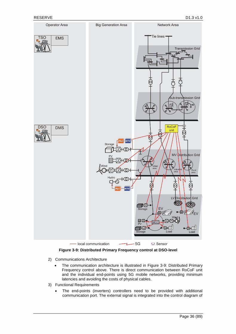
RESERVE D1.3 v1.0

(89)

Figure 3-9: Distributed Primary Frequency control at DSO-level


• The communication architecture is illustrated in Figure 3-9: Distributed Primary Frequency control above. There is direct communication between RoCoF unit and the individual end-points using 5G mobile networks, providing minimum latencies and avoiding the costs of physical cables.


• The end-points (inverters) controllers need to be provided with additional communication port. The external signal is integrated into the control diagram of

RESERVE D1.3 v1.0

(89)

the inverter. Some end-points of larger power can include an RTU, and thus the control signal is not directly sent to the inverter.

• As the primary control requires deployment of the power reserve between 5 and 30 seconds, the entire chain of measurement, data collection, data processing and communication should be done within few seconds.









DSO, Distributed Control, Sf_B


• On DSO-level, there are up to thousands of individual end-points including flexible loads, prosumers, and storage systems. The end-points are located in LV and MV distribution networks that will participate in frequency control mechanisms. Please see Figure 3-10: Distributed Primary Frequency Control at DSO-level below.

• The prosumers and microgrids will contribute with frequency stabilization.

• The frequency estimation and measurements could be executed in distributed areas, and their signals will be provided to the respective primary controllers.

• The RoCoF signal is used together with the Δf signal for primary frequency control. In this case, it is assumed that the RoCoF signal is not local, but obtained from a regional RoCoF unit.

RESERVE D1.3 v1.0

(89)

Figure 3-10: Distributed Primary Frequency Control at DSO-level


• The communication architecture is illustrated in Figure 3-10: Distributed Primary Frequency Control at DSO-level above. There is direct communication between RoCoF unit and the individual end-points using 5G mobile networks, providing minimum latencies and avoiding the costs of physical cables. Also, there will be coordination links between the distributed controllers for primary frequency management.


• The end-points (converters’ controllers) need to be provided with additional communication port. The external signal is integrated into the control diagram of the converter.

• As the primary control requires deployment of the power reserve within less than 10 seconds (approx. in 5 seconds), the entire chain of measurement, data collection, data processing and communication should be done in a very fast manner accordingly.


• Latency: as the functional requirements indicate above, extremely short latencies help to provide the best control consistency in the grid. One complete cycle including measurements, data analysis and control response should be executed in very less than one second.

• Jitter can alter the quality of the control if the control signal is delayed by one second.



• Authentication: all parties in the communication should use the latest authentication processes according to the latest security standards defined by

RESERVE D1.3 v1.0

(89)

IEEE, IEC and other prominent standardisation bodies. Authentication techniques can be leveraged from future 3GPP (5G) mobile communication standards such as Generic Bootstrapping Architecture (GBA).



3.1.3 Secondary Control

TSO, Centralised Control, Sf_A

There is no need for DSO-level Secondary Frequency Control in Sf_A.


• This type of control is an upgraded system of the secondary frequency control employed today. Besides the classical power plants, and in SF_A only hydraulic power plants are considered, new entities will be used such as virtual power plants and microgrids.

• Virtual power plants and microgrids are the new actors and solutions to efficiently coordinate the stochastic and/or small-scale generation, storage, and load entities in order to provide power and load reserved for system balancing. These features are needed in power systems lacking hydraulic power plants, while the storage systems are not sufficiently available to provide the required amount of energy. Alternatively, virtual power plants and microgrids can also be used in the tertiary frequency control level to achieve economic goals including optimal economic dispatch of energy.

• A basic scheme for the secondary frequency control, coordinated by the TSO, is Figure 3-11. The DSO should not have any role here, except for sharing its communication infrastructure in some use cases.

• Independent energy storage systems are considered on this level of control. Their communication with the AGC is similar to all other controlled generation units.

• Information regarding the available reserve bands is uploaded manually in the AGC application by the power market operator, using an easy-to-use software application.

• The instantaneous power provided by all controlled entities (generation units, storage systems, VPPs or microgrids) is monitored by means of the power generation application, which is also a component of the EMS. In case of large unbalances caused by erroneous operation of a controlled entity followed by the 100% use of the secondary reserve band, the human operator will proceed to manually deployment (phone call) of the tertiary reserve in emergency conditions. If critical frequency deviations occur, the automatic load shedding systems will trigger load disconnection so that the stability of the power system is maintained.

RESERVE D1.3 v1.0

(89)

Figure 3-11: Centralised Secondary Frequency Control, TSO-level


• The overall number of connections is highly limited in the future, as the TSO EMS will communicate with the VPP or microgrid control centres, avoiding the need of exchanging data with every small-scale generation unit.

• For those generation resources provided with RTU, the glass-fibre integrated into the optical ground wire (OPGW) of the transmission and distribution lines is used for direct communication with the TSO. Glass-fibre is also used to collect power flows data from the tie-lines to the EMS of the TSO.

RESERVE D1.3 v1.0

(89)

• In the case of virtual power plants and microgrid entities, there are two levels of communication: 1. glass-fibre is used for communication between the TSO and the VPP Control Centre (VPPCC) or the Microgrid Control Centre (MGCC); 2. VPN over Internet using private infrastructures is used for communication between the VPPCC and MGCC and the controlled resources.

• The high-level coordination is provided from the AGC. Based on various input data, including one frequency value and several power values, the AGC calculates the control signals to be sent to the controlled generation units.

• Low-level coordination exists at the VPP and microgrid levels. Based on the signal order received from the AGC, and various economic and technical data of their resources, the VPPCC and MGCC determine the level of power increase or decrease for each generation resource.

• Availability of the VPP and microgrid to participate in the secondary frequency control is known in advance, typically one day before, and updated if necessary in real-time, typically one hour before.


• AGC, or automatic generation control, is a software application of the EMS. It performs all necessary calculations using block diagrams to determine the necessary corrections including upward and downward regulation to be done by the controlled generation units of aggregators.

• Two types of data are used in the AGC function:

i. Frequency data, measured by means of a GPS-synchronized frequency-meter in the LV grid of the building where the EMS-SCADA system is located. The measurement error is usually standardized.

ii. Active power flows on the tie lines, called also interchange power. The EMS server collects all these data from the RTUs installed in the power substation of all tie-lines. The measurement error is usually standardized.

• The refresh rate of data of the AGC is 2 seconds.

• The metering equipment in the substations are the current transformer and the

voltage transformer. The metered data, i.e. voltage and current, is sent to the

local RTU, which calculates the active power.

• Each generation unit is equipped with an RTU for local data acquisition from the

metering equipment, formatting the data into a standardized form and sending

the data to the EMS. The measurement-receiving-decoding data cycle of an RTU

is 4-6 seconds.

• The AGC cycle is 4 seconds. A control signal is sent from the EMS to all controlled

entities only if necessary; if the frequency and the power exchanges are within

acceptable deviation, then no control signal is sent. For this reason, the

calculation and communications inside the VPPs and the microgrids must be

completed in less than 4 seconds.


• Latency: the high-level coordination can remain similar to the systems in use today. However, when VPPs and microgrids are used, faster internal communication in these subnetworks is required. Note that all measurements still have to be collected rather quickly in less than 1 second, as in primary control.

• In secondary frequency control, the system is designed to restore the frequency to the nominal value by balancing the powers. The maximum standard time for accomplishing this is 15 minutes. If the unbalance is smaller, then the frequency is restored faster. Even delays of 1-2 seconds are acceptable in this context, and limited amounts of jitter cause no disturbance of the solution overall.

• Data Volume/Bandwidth: in the future, tens of control signals corresponding to the generation entities could be sent at the same time on this control level, while data from 10 to 20 power flows are received from the tie-lines. Therefore, only a small number of data elements (max 1 kByte each) multiplied by tens of entities need to be sent every 2 to 4 seconds.

RESERVE D1.3 v1.0

(89)


• At the higher-level coordination, there two unidirectional communications. First, the EMS receives frequency and power flow data from the grid. Secondly, control signal is sent to the controlled entities. Entity identification is ensured through hardware-software configurations.

• No data encryption is required, when the communication system operates in a closed loop. If public or shared communication networks are used, the data has to be encrypted to prevent misuse or external interference with the measurements and control commands.

• For some transmission system operators, the communication system will operate in a closed loop. In this case, security can be ensured by carefully closing the external communication ports. If there is erroneous operation of a controlled entity to produce power unbalances of frequency deviations, other control levels will counteract the effect. However, erroneous operation of a single entity will not have immediate critical effects on the power system operation.

• The state estimation application, which is a component of the EMS, determines the erroneous data and provides estimations instead. The EMS-SCADA is a redundant system; there is redundancy for all data and equipment.

TSO, Centralised Control, Sf_B


• This type of control is an upgraded system of the secondary frequency control employed today. New entities will be used such as virtual power plants and aggregators.

• The new entities represent a promising solution to efficiently coordinate their power generation in order to participate with power balancing and frequency stabilization.

• A basic scheme for the secondary frequency control, coordinated by the TSO, is available in Figure 3-12: Centralised Secondary Frequency Control at TSO-level.

• Independent energy storage systems are considered on this level of control. Their communication with the AGC is similar to all other controlled generation units.

• Information regarding the available reserve bands is uploaded manually in the AGC application by the power market operator, using an easy-to-use software application.

• The instantaneous power provided by all controlled entities (generation units, storage systems, VPPs or microgrids) is monitored by means of the power generation application, which is also a component of the EMS.

RESERVE D1.3 v1.0

(89)

Figure 3-12: Centralised Secondary Frequency Control at TSO-level


• The overall number of connections is highly limited in the future, as the TSO EMS will communicate with the VPP or aggregators.

• For those generation resources provided with RTU, the glass-fibre integrated into the optical ground wire (OPGW) of the transmission lines is used for direct communication with the TSO. Glass-fibre is also used to collect power flows data from the tie-lines to the EMS of the TSO.

• In the case of virtual power plants, there are two levels of communication: 1. glass-fibre is used for communication between the TSO and the VPP Control Centre (VPPCC) 2. VPN over Internet using private infrastructures is used for communication between the VPPCC and the controlled resources.

• The high-level coordination is provided from the AGC. Based on various input data, including one frequency value and several power values, the AGC calculates the control signals to be sent to the controlled generation units. The frequency estimation and measurements could be different in every area in the network. Hence, several frequency measurements units will be distributed in the network

• Low-level coordination exists at the VPP level. Based on the signal order received from the AGC, and various economic and technical data of their resources, the VPPCC determine the level of power increase or decrease for each generation resource.

• Availability of the VPP to participate in the secondary frequency control is known in advance, typically one day before, and updated if necessary in real-time, typically one hour before.


• AGC, or automatic generation control, is a software application of the EMS. It performs all necessary calculations using block diagrams to determine the

RESERVE D1.3 v1.0

(89)

necessary corrections including upward and downward regulation to be done by the controlled generation units of aggregators.

• Two types of data are used in the AGC function:

i. Frequency data, measured by means of a GPS-synchronized frequency-meter.

ii. Active power flows on the tie lines.






the data to the EMS.

• A control signal is sent from the EMS to all controlled entities only if necessary; if

the frequency and the power exchanges are within acceptable deviation, there is

no control signal to be sent, and hence, there is no need for frequency control

activation.


• Latency: the high-level coordination can remain similar to the systems in use today. However, when VPPs are used, faster internal communication in these subnetworks is required. Note that all measurements still have to be collected rather quickly in less than 1 second, as in primary control.

• In secondary frequency control, the system is designed to restore the frequency to the nominal value by balancing the powers. The maximum standard time for accomplishing this is way less than 10 minutes. A short delay within a second are acceptable in this context, and limited amounts of jitter cause no disturbance of the solution overall.

• Data Volume/Bandwidth: in the future, tens of control signals corresponding to the generation entities could be sent at the same time on this control level, while data from 10 to 20 power flows are received from the tie-lines. Therefore, only a small number of data elements (max 1 kByte each) multiplied by tens of entities need to be sent every approx. 1-2 seconds.


• At the higher-level coordination, there two unidirectional communications. First, the EMS receives frequency and power flow data from the grid. Secondly, control signal is sent to the controlled entities. Entity identification is ensured through hardware-software configurations.

• No data encryption is required, when the communication system operators in a closed loop. If public or shared communication networks are used, the data has to be encrypted to prevent misuse or external interference with the measurements and control commands.

• For some transmission system operators, the communication system will operate in a closed loop. In this case, security can be ensured by carefully closing the external communication ports. If there is erroneous operation of a controlled entity to produce power unbalances of frequency deviations, other control levels will counteract the effect. However, erroneous operation of a single entity will not have immediate critical effects on the power system operation.

• The state estimation application, which is a component of the EMS, determines the erroneous data and provides estimations instead. The EMS-SCADA is a redundant system; there is redundancy for all data and equipment.

DSO, Centralised Control, Sf_A

In scenario Sf_A, the DSO will not have an active role in the secondary control level. This is due to economic reasons. From the security point of view, one coordinator of this control level is enough.

RESERVE D1.3 v1.0

(89)

DSO, Centralised Control, Sf_B


• A new control and communication architecture will be developed for secondary frequency control in DSO. This will coordinate with the local controllers within distribution network from one hand, and with the respective TSO from the other hand. New entities will be included such as virtual power plants and aggregators.

• The new entities represent a promising solution to efficiently coordinate their power generation in order to participate with power balancing and frequency stabilization in DSO level.

• A basic scheme for the secondary frequency control at DSO level is illustrated in Figure 3-13: Centralised Secondary Frequency Control at DSO-level.

• The instantaneous power provided by all controlled entities (generation units, storage systems, VPPs or microgrids) is monitored by means of the power generation application, which is also a component of the DMS.


• The overall number of connections will be high, as the DMS will communicate with the VPP, aggregators, and prosumers/microgrids.

• The Secondary Frequency Control (SFC) could be allocated in/coordinated with SSAU.

• The high-level coordination is provided from the SFC. Based on various input data, including one frequency value and several power values, the SFC calculates the control signals to be sent to the controlled generation units. The frequency estimation and measurements could be different in every area in the network, depends on the location of faults/perturbation. Hence, several frequency estimation and measurements units will be installed in different areas in the network

• Low-level coordination exists at the VPP level. Based on the signal order received from the SFC, and various economic and technical data of their resources, the VPPCC determine the level of power increase or decrease for each generation resource.


• Within DMS, all necessary calculations are executed using block diagrams to determine the necessary corrections including upward and downward regulation to be done by the controlled generation units of aggregators.

• The frequency data, measured by the frequency estimation/divider, is send to the SFC.




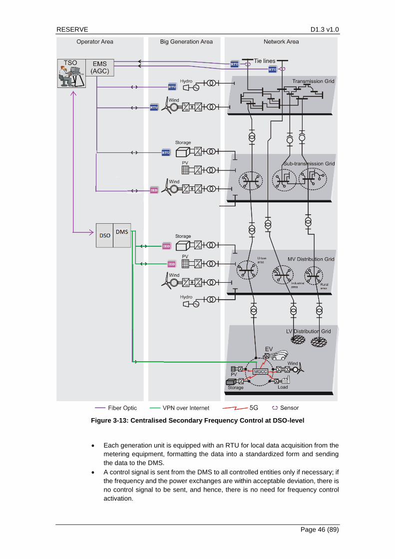
RESERVE D1.3 v1.0

(89)

Figure 3-13: Centralised Secondary Frequency Control at DSO-level



the data to the DMS.

• A control signal is sent from the DMS to all controlled entities only if necessary; if

the frequency and the power exchanges are within acceptable deviation, there is

no control signal to be sent, and hence, there is no need for frequency control

activation.

RESERVE D1.3 v1.0

(89)


• Latency: the high-level coordination can be used. However, when VPPs are used, faster internal communication inside these subnetworks is required. Note that all measurements still have to be collected rather quickly in less than 1 second, as in primary control.

• In secondary frequency control, the system is designed to restore the frequency to the nominal value by balancing the powers. The maximum standard time for accomplishing this is way less than 10 minutes. A short delay within a second are acceptable in this context, and limited amounts of jitter cause no disturbance of the solution overall.

• Data Volume/Bandwidth: in the future, tens of control signals corresponding to the generation entities could be sent at the same time on this control level, while data from 10 to 20 power flows are received from the tie-lines. Therefore, only a small number of data elements (max 1 kByte each) multiplied by tens of entities need to be sent every approx. 1-2 seconds.


• At the higher-level coordination, there two unidirectional communications. First, the DMS receives frequency and power flow data from the grid. Second, control signal is sent to the controlled entities. Entity identification is ensured through hardware-software configurations.

• A coordination framework will be created between TSO and DSO for frequency regulation in overall network. This will lead to the appearance of new roles, activities, and control-communication requirements.

• For some distribution system operators, the communication system will operate in a closed loop. In this case, security can be ensured by carefully closing the external communication ports. If there is erroneous operation of a controlled entity to produce power unbalances of frequency deviations, other control levels will counteract the effect. However, erroneous operation of a single entity will not have immediate critical effects on the power system operation.

• The state estimation application, which is a component of the DMS, determines the erroneous data and provides estimations instead.

3.2 Voltage Control Scenarios

3.2.1 DSO, Dynamic Voltage Stability Monitoring (Sv_A)


Today’s Low-Voltage Grids

In today’s low-voltage grids, the distribution grid consists of a Secondary Substation Automation Unit (SSAU) from which radial feeders are available. The loads consisting of small industries and households are connected to these radial feeders as depicted in Figure 3-14 below. Typically, due to lack of dynamic voltage control concepts in the loads, the loads can be represented as fixed impedances. The nodes at which the local loads are connected to the radial LV feeder is denoted as the point of common coupling (PCC) local to the load. The impedance present in the feeder between two local PCCs is also depicted in the figure as 𝑍𝑐1, 𝑍𝑐2 etc. The impedance of the feeder is due to the resistance of the cables and the inductance of the cable. In this simple structure, power flow is always unidirectional where power flows from the SSAU to the loads through the radial LV feeder. There is no real power injection from the load side into the LV feeder through the local PCC in the classical picture. Control is achieved by adjusting the turns ratio of the on-load tap changing transformer (OLTC) in the SSAU.

RESERVE D1.3 v1.0

(89)

Figure 3-14: Classical Power System Structure

Future Low-Voltage Grids

In future low-voltage grids, the structure of an LV grid is portrayed by 100% RES scenario. Many households will have their own RES, and a grid-connected inverter. With the development of LED-based illumination technology, the lighting loads would be DC-based. Similarly, household loads which involve electric motors are moving towards brushless technology and DC. Brushless DC motors and permanent magnet synchronous motors are of prime focus for the future, and these motor technologies require a DC bus connection. A feedback-controlled inverter is integrated with the motor within a single enclosure and this concept is known as integrated motor drive (IMD) technology.

Furthermore, the increased popularity of electric vehicles and its corresponding DC technology for battery charging systems would increase the concentration of DC loads in the grid. Rectifiers which convert AC to DC are used to interface the LVAC feeder with the above-mentioned examples of futuristic DC loads. The DC loads are represented with blue, rectifiers in yellow, inverters in green and AC loads in red in Figure 3 2: Futuristic power system structure. The futuristic scenario will mostly likely have DC loads, however to respect the existing debate, a few AC loads in red are also depicted. The new buildings to be built in the future would be built as DC homes. However, in existing buildings, it will be advantageous when appliances are slowly replaced to DC instead of converting the entire residential network to DC in a single step. Hence, the case of hybrid AC/DC homes are considered without loss of generality.

The benefit of Sv_A is its ability to provide stability in grids with highly dynamic loads.

Figure 3-15: Layout of Future Low-voltage Gris

Threat to Stability

The presence of constant power loads (CPL) is a potential voltage stability threat to power systems. The grid connected active rectifiers regulate the DC supply voltage for DC homes in the future. At a given point in time, for a given amount of load present in the house, these rectifiers take constant power from the grid independent of the voltage magnitude, thus exhibiting a CPL behaviour. Thus, due to a random load switching event, when the bus voltage goes down, the current drawn by these CPL increases further affecting the grid voltage. Hence when large proportions of these CPLs are going to be installed in future grids, the bus voltage stability will

MV/LVSSAU

Zc1 Zc2 Zc3PCC1 PCC3PCC2

RESERVE D1.3 v1.0

(89)

become critical. The threat of oscillations and other interactions between the inverter and the rectifier needs to be addressed.

List of possible actors involved in the scenario

DSO will operate the SSAU and is the key driver for voltage management. The microgrid operator is likely to play the same role as a DSO in the voltage scenario context. The Microgrid operator can perform Sv_A on the inverters which are in the Microgrid and appear as a single stable operating point source to the DSO in the larger realm. An aggregator might not have role in this scenario since the aggregator is distributed across the country.


The SSAU, which is located in the secondary substation, coordinates the inverters for impedance measurements. The SSAU gathers impedance information per inverter on an hourly basis. Each inverter has its own WSI tool and a VOI controller. The inverter also has communication ports to communicate with the SSAU. The SSAU commands the inverters WSI tool for initiation of impedance measurement and then inverter responds back with the impedance data. Hence the communication from WSI to SSAU is bidirectional. The corrective actions are sent from the SSAU to the VOI controller. Thus, a unidirectional communication from SSAU to VOI controller is required.

There is no “counterpart” or comparable concept in today’s MV/LV feeder networks.

RESERVE D1.3 v1.0

(89)

Figure 3-16: Voltage Control, Dynamic Voltage Stability Monitoring


a) The Sv_A algorithm, that is the dynamic voltage stability monitoring algorithm, which exists as a software component in the SSAU, requires the impedance information of the grid and the inverter at each inverter connection point. Therefore, communication to the inverter is required. Furthermore, when the evaluated stability margins are low, corrective actions need to be sent to each VOI controller of the inverter for which communication links are required.

b) Impedance data need to be sent, i.e coefficients of the numerator and denominator polynomial of the impedance transfer function. The impedance of the inverter and grid is required to study the stability based on Middlebrook theory. The margins of stability are also determined using the impedance information.

c) The data exchange takes place approx. once every hour. So, data will be transmitted once an hour from SSAU to inverter to request impedance data from all end-points in the local grids. The Inverters respond back with impedance measurements. After analysing the input data, the SSAU might give commands

RESERVE D1.3 v1.0

(89)

to the VOI controller to correct the impedance in the local environment. The exact format of these control messages is not known, as the VOI controller is still under development. It will be analysed in later deliverables. For further details on the process, please see chapter 8.2.2.2 SGAM Information Layer: Data Model below.

d) The measurement data and the corrective actions, that are generated once an hour, have to be stored by the S.SAU for several hours to be able to locate end-points with persisting problems at a later point. Furthermore, some statistics will be extracted from this data.


a) Latency: in current solutions, voltage stability monitoring is planned on an hourly basis, it is not continuously ongoing. Still, latency is a critical factor to ensure that the voltage control process is completed in a few seconds, including data transmission and processing. The faster the process is carried out, the quicker the voltage level will be corrected. Simulations later in the project will provide more exact latency requirements.

b) Jitter: Jitter does not create any significant problems in this scenario, as every end node or point is treated individually. The SSAU requires the inverter to measure its output impedance and the grid impedance. Thus, in this highly decentralised approach, jitter does not create problems.

c) Data Volume/Bandwidth: in a typical low voltage feeder grid, 1,000 to 10,000 inverters are monitored by one SSAU. So, this realistic prerequisite helps to determine the overall data volume for the solution. Consider the following assumptions and calculations:

• Floating point (double precision) – 8 bytes per number

• Number of floating point numbers per inverter – 40

• Number of inverters (1 Inverter per end-point) – 10,000

• Kilobytes per second – 8*40*10,000/(1024*3600) = 1.736 kBytes/s

• Kilobits per second – 13.88 kbits/s


Authentication: each inverter needs a unique address to communicate with neighbouring inverters, as well as the SSAU. This is similar to the meter point reference number, MPRN, identifying smart meters in a country gathered in a database. The inverters and end-points are stationary, the DSO would maintain an internal database of end-points, inverters and whether they are located next to each other.

Data Encryption: it is essential to encrypt both impedance measurements as well as commands for voltage control. Since any corruption of data might lead to faulty impedance mapping, resulting in faulty computation of stability margins in the SSAU. This would cause invalid target impedance values to be sent to the VOI controllers of inverters, causing severe instability that might disturb the LV breakers in the LVAC grid, and possibly cause an outage of the entire system.

Data integrity: it is important to validate the voltage control commands upon reception, to ensure that they were not tempered with during transmission.

In addition, it is recommended to keep the physical or street address of any end-point confidential, and should not be online mapping between IP address and geographical address. Therefore, physical addresses and other sensitive household-based data should not be transmitted over the communications network at any time.

3.2.2 DSO, Decentralised Control, Sv_B


At present, management of voltages on distribution networks is achieved through the coordination of on-load tap-changers (OLTC), transformers, capacitor banks, series reactors, Static VAr Compensators (SVC) and static synchronous compensators (STATCOM), see D3.1 for more details on these concepts. These are

RESERVE D1.3 v1.0

(89)

primarily installed and operated at MV distribution system level. On LV networks, there is sufficient headroom for voltage drop from the control of voltages in MV networks, assuming of course that only demand is being drawn on the networks. The last mile of network is unmonitored, save for the customer premises kWh usage. Unrestricted connection of RES could potentially cause voltage or thermal problems that could go undetected.

The future scenario will change the status-quo from a network with passive voltage management to a scenario where consumers and prosumers actively contribute to the management of voltages in their surrounding network. In Sv_B a voltage measurement is foreseen at every point where an inverter-based RES unit is connected. This new voltage control scheme will not replace the present management. Instead, the present system will remain in service and take precedence and provide the basic platform for Sv_B. It is anticipated that the inverter-based RES units would inject and absorb reactive power based upon their observed terminal voltage. Each unit will be tuned to follow a predefined volt-VAr curve, stipulated by an objective: for instance, the minimisation of active power losses.

Figure 3-17: Principal architecture for Sv_B

Such a scenario could invoke a request from a TSO or DSO to engage the RES units in an area of the network toward a singular objective. This capability suggests that the role of an aggregator in providing both a commercial service as well as a technical service. This aggregator could engage the response of multiple inverters (consumers and prosumers), a microgrid or operate a number of secondary substation automation units (SSAU).


SV_B removes the requirement of calculating an updated AC power flow simulation at every iteration. Reducing the offline centralised analysis to an online and decentralised deployment through the means of optimally chosen volt-VAr curves, gives a practical means to facilitate the objectives of the DSO. The communications architecture required is a measurement of voltage at the terminals of every inverter based RES unit tuned with a volt-VAr curve, a link to the SSAU, the DSO EMS and potentially an interaction to the TSO is also relevant.

For more details see Figure 2-6: Decentralised Voltage Control with Technical Aggregator above.


There are two possibilities for implementing the active voltage management technique. In one case, the measurement of voltage is communicated to the SSAU, corrective action is calculated at the SSAU and an instruction for a change in reactive power is then communicated to the RES unit. A second possibility is a shift towards complete autonomy of control. In this second case, the control action for a change in reactive power is calculated locally based on a local voltage measurement (and possibly the voltage measurement at the secondary substation). This would reduce the role of the SSAU to receive and send the required volt-VAr curve (defined by the objective of the DSO/TSO in that instant) to the RES units in question. In either case the architecture is unaltered, but the functional requirements of the components are altered. In either case, a new generation of inverters is required with communication capabilities.

RESERVE D1.3 v1.0

(89)

The calculation of required change in reactive power must adhere to the technical limitations of the inverter to provide reactive power while also enforcing the grid codes relevant to the jurisdiction of the RES unit. This functionality must be coded into the process of following the volt-VAR curve.

The type of data to be sent in either case is a floating-point number made up of 32bits, describing the voltage measurement and required reactive power set point operation. For autonomous control, the target voltage (intercept) and slope of the volt-VAr corresponding to the objective of the DSO would need to be communicated also.

The time frames of communication are dependent on the mode of operation; continuous or threshold operation is possible. Table 3-1: Modes of Operation of Sv_B Voltage Control describes both modes of operation and provides an indication for the frequency of communication.

Table 3-1: Modes of Operation of Sv_B Voltage Control

Operation Description Time Frames

Continuous

Voltage is managed on a continuous basis. Communication of local voltage

measurement takes place regardless of whether the voltage target changes.

1 - 5 seconds

Threshold

Voltage is managed within a threshold whereby the target voltage of the RES unit can deviate within bounds, only

when outside this bound would communication be required for a control

action to be taken.

Network dependant. A time frame of minutes is possible at times

where consumers/prosumers are static, e.g. during the night


The round-trip time of a complete cycle from the inverter to the point of calculation and back is important. The quicker the measurement and the required change can be communicated the more accurate and effective the control action. The latency requirements for SV_B are in the region of 10ms. In order to facilitate the connection of RES up to 100%, the faster the round-trip time for the AVM technique the better: this will make best use of, and maximise the finite capacity of, distribution networks at all times.

In relation to Jitter, the voltage control action should consider the most recent and valid signal when performing a calculation. The latest available values should be used. The total throughput for a single inverter-based RES unit is approximately 500 bytes every second, considering the higher frequency in continuous operation. For an SSAU connecting 500 customers, the throughput would be 500 * 500 = 250kBytes/s or 15MBytes/min.


For the sake of protecting customer and user privacy security in terms of authentication, encryption and integrity are all of importance to data transmission in distribution systems. A sanity check at the point of calculation for corrective action, would be good practice and important if the voltage is to be maintained within the bounds stipulated by the network grid codes. At no time should a command for a device to operate outside limits be issued, such a command could damage the lifetime of the asset and cause harm to the behaviour and objective of the use case.

RESERVE D1.3 v1.0

(89)

4. References

Deliverable D1.1 [RESERVE]

Deliverable D1.2 [RESERVE]

1. European Network of Transmission System Operators for Electricity (ENSOE), Network Code Development, Available online: https://www.entsoe.eu/major-projects/network-code-development/updates-milestones/Pages/default.aspx

2. ESB Networks, Distribution Code, Version: 5.0, April 2016. Available online: https://www.esbnetworks.ie/docs/default-source/publications/distribution-code-v5-0.pdf?sfvrsn=6

3. EirGrid, Grid Code, Version 6.0, 22nd July 2015. Available online: http://www.eirgridgroup.com/site-files/library/EirGrid/GridCodeVersion6.pdf

4. Commission Regulation (EU) establishing a guideline on electricity transmission system operation, draft 2016. Available online: https://ec.europa.eu/energy/sites/ener/files/documents/SystemOperationGuideline%20final%28provisional%2904052016.pdf

5. TEL-07.V OS-DN/280, Procedura operationala – Verificarea functionarii grupurilor hidroelectrice si termoelectrice in reglaj primar (eng.: Operation procedure – Verification of hydroelectric and thermoelectric units operation in primary control). Available online: http://www.transelectrica.ro/documents/10179/146969/Verificarea+functionarii+grupurilor+hidro+si+termo+in+reglaj+primar_TEL+07.V+OS-DN-280_dec2010.pdf/ff4ae061-ab1c-449a-b1f9-f1dd118db079

6. TEL-07.V OS-DN/190, Procedura operationala – Verificarea functionarii grupurilor hidroelectrice si termoelectrice in reglaj secundar (eng.: Operation procedure – Verification of hydroelectric and thermoelectric units operation in secondary control). Available online: http://www.transelectrica.ro/documents/10179/29755/Procedura_Echilibrare_Avizate_28-12-2010_7qvq.pdf/d7df7bbc-d4e7-4a88-9590-c38d1fda8185

7. TEL-07V OS-DN/154, Procedura operationala - Calificarea furnizorilor de servicii tehnologice de sistem (eng.: Operation procedure – Qualification of the ancillary services suppliers). Available online: http://www.transelectrica.ro/documents/10179/42218/Procedura_STS_Avizate_14-07-2010_c00s.pdf/6f9fb0a1-c8eb-4dc0-b0d3-57c41a610107

8. Ordin ANRE 72/2.08.2017 pentru aprobarea Normei tehnice privind cerinţele tehnice de racordare la rețelele electrice de interes public pentru grupurile generatoare sincrone (ANRE Decision 72/2.08.2017 for approval of the technical norm regarding the technical requirement for connection to the public grid of the synchronous generator unit). Available online: http://213.177.15.183/PublicLists/Ordin

9. Cod ANRE: 51.1.112.0.01.27/08/04, Codul Tehnic al Retelei Electrice de Transport (eng.: The technical code of the transmission electrical network). Available online: http://www.transelectrica.ro/documents/10179/33158/cod_ret_ro.pdf/5cf5bb39-2efb-48f7-9ebc-491dfdb7d6e0

10. IEC 60870-5-101:2003+AMD1:2015 Standard “Telecontrol equipment and systems-Part 5-101: Transmission protocols – Companion standard for basic telecontrol tasks”.

11. IEC 61850-7-2:2010, Communication networks and systems for power utility automation - Part 7-2: Basic information and communication structure - Abstract communication service interface (ACSI).

12. IEC 61850-7-420:2009 Communication networks and systems for power utility automation - Part 7-420: Basic communication structure - Distributed energy resources logical nodes

13. IEC 61850-8-1:2011, Communication networks and systems for power utility automation - Part 8-1: Specific communication service mapping (SCSM) - Mappings to MMS (ISO 9506-1 and ISO 9506-2) and to ISO/IEC 8802-3

14. IEC 61850-9-2:2011, Communication networks and systems for power utility automation - Part 9-2: Specific communication service mapping (SCSM) - Sampled values over ISO/IEC 8802-3

https://www.entsoe.eu/major-projects/network-code-development/updates-milestones/Pages/default.aspx

https://www.entsoe.eu/major-projects/network-code-development/updates-milestones/Pages/default.aspx

https://www.esbnetworks.ie/docs/default-source/publications/distribution-code-v5-0.pdf?sfvrsn=6

https://www.esbnetworks.ie/docs/default-source/publications/distribution-code-v5-0.pdf?sfvrsn=6

https://ec.europa.eu/energy/sites/ener/files/documents/SystemOperationGuideline%20final%28provisional%2904052016.pdf

https://ec.europa.eu/energy/sites/ener/files/documents/SystemOperationGuideline%20final%28provisional%2904052016.pdf

http://www.transelectrica.ro/documents/10179/29755/Procedura_Echilibrare_Avizate_28-12-2010_7qvq.pdf/d7df7bbc-d4e7-4a88-9590-c38d1fda8185

http://www.transelectrica.ro/documents/10179/29755/Procedura_Echilibrare_Avizate_28-12-2010_7qvq.pdf/d7df7bbc-d4e7-4a88-9590-c38d1fda8185

http://www.transelectrica.ro/documents/10179/42218/Procedura_STS_Avizate_14-07-2010_c00s.pdf/6f9fb0a1-c8eb-4dc0-b0d3-57c41a610107

http://www.transelectrica.ro/documents/10179/42218/Procedura_STS_Avizate_14-07-2010_c00s.pdf/6f9fb0a1-c8eb-4dc0-b0d3-57c41a610107

http://213.177.15.183/PublicLists/Ordin

http://www.transelectrica.ro/documents/10179/33158/cod_ret_ro.pdf/5cf5bb39-2efb-48f7-9ebc-491dfdb7d6e0

http://www.transelectrica.ro/documents/10179/33158/cod_ret_ro.pdf/5cf5bb39-2efb-48f7-9ebc-491dfdb7d6e0

RESERVE D1.3 v1.0

(89)

5. Open Issues and Items for Future Research

• Role of aggregators in frequency and voltage control

• Role of VPPs in frequency and voltage control

RESERVE D1.3 v1.0

(89)

6. Conclusion

This document describes the relationship between the power network architectures being considered by the project for the frequency and voltage control scenarios of RESERVE and the ICT architectures and capabilities needed to implement them.

Given that the most critical application of grid stabilisation deals with frequency control, which will impact at three different time scales, inertial, primary control, and secondary control, this area was looked at first from the point of view of two different approaches labelled Sf_A, Mixed Mechanical-Synthetic Inertia, and Sf_B, Full Synthetic Inertia.

From a power network architecture perspective, it was observed that the main differences between Sf_A and Sf_B are in terms of system generation, inertia, dynamics, and control time window. In addition, very fast and reliable communication is more critical in Sf_B than in Sf_A.

It was also found that there was no difference in the control architecture between Sf_A and Sf_B. In other words, both scenarios could have: decentralised and distributed control for inertial and primary control, and centralised for secondary control.

In setting the ICT requirements for the frequency control scenarios the functional, performance and security requirements were explored for the Sf_A and Sf_B scenarios.

Minimum transmission and computation times of less than 0.5 seconds and maximum data volume/bandwidth of 100 MByte for one hour of measurements were unearthed. Also, extremely short latencies where shown to provide the best possible control when it comes to frequency.

While it was found that only Kbytes of data would be transferred from measuring units, the sheer number of end-points (hundreds, up to thousands) would be a major cause for consideration of ICT communication architecture and requirements.

Security concerns centred around authentication and authorisation especially given the impact that would happen if there were malicious modification of the measurement data and commands sent to end-point controllers.

In the evolution towards 100% RES, the objective of voltage control is to balance the voltage in future low voltage distribution grids connecting local loads and prosumers as well as energy storage facilities. The aim is to stabilize the voltage as local as possible, so that decisions and control commands can be issued as quickly as possible. Consumers and prosumers should not experience any disturbances of their power supply. Towards this aim the RESERVE project is looking at two different approaches to voltage stability, labelled Sv_A: Dynamic Voltage Stability Monitoring and Sv_B, Active Voltage Management.

From the power architecture perspective, it was observed that the main differences between Sv_A and Sv_B were in terms of Sv_A dealing with a timeframe of response in the order of milliseconds whereas Sv_B was of the order of minutes. Also, Sv_A requires that a WSI tool, VOI controller and communication ports in the inverter are added, whereas Sv_B can use existing data being measured from the field. The SSAU is an important component in both approaches.

In setting the ICT requirements for the voltage control scenarios the functional, performance and security requirements were also extensively explored for the Sv_A and Sv_B scenarios.

Minimum transmission and computation times in the order of milliseconds and maximum data volume/bandwidth of 15 MBytes/s were unearthed. Although latency was less of an issue when it comes to voltage control scenarios.

Again, while it was found that in a number of cases only Kbytes of data would be transferred by measuring units, the sheer number of end-points (10,000) would be a major cause for consideration of ICT communication architecture and requirements.

Security concerns centred around authentication, data encryption and data integrity.

For all the scenarios, frequency (Sf_A, Sf_B) and voltage (Sv_A, Sv_B) the ICT communications architecture was considered with a focus placed on the use of 5G wireless communications capabilities where it was appropriate. Future ICT solutions offer great opportunities for instant corrective actions for monitoring and control and the deeper impact of these solutions for frequency and voltage stability will be explored in the D2.4 and D3.6 deliverables of RESERVE.

RESERVE D1.3 v1.0

(89)

7. List of Abbreviations

AGC Automatic Generation Control

B2B Business to Business

BMS Building management system

CENELEC European Committee for Electro technical Standardization

CEP Complex Event Processing

CPMS Charge Point Management System

Δf Amount of change of frequency

DER Distributed Energy Resources

DMS Distribution Management System (DSO domain)

DSE Domain Specific Enabler

DSO Distribution System Operator

EAC Exploitation Activities Coordinator

EMS Energy Management System (TSO domain)

ESB Electricity Supply Board

ESCO Energy Service Companies

ESO European Standardisation Organisations

ETSI European Telecommunications Standards Institute

HV High Voltage

ICT Information and Communication Technology

IEC International Electro-technical Commission

IoT Internet of Things

KPI Key Performance Indicator

LV Low Voltage

M2M Machine to Machine

MG Microgrid

MGCC Microgrid Control Centre

MPLS Multiprotocol Label Switching

MV Medium Voltage

NIST National Institute of Standards and Technology

OPGW Optical Ground Wire

OPEX Operational Expenditure

O&M Operations and maintenance

PLC Programmable Logic Controller

PPP Public Private Partnership

PV Photovoltaic (power generation unit)

RTU Remote Terminal Unit

S3C Service Capacity; Capability; Connectivity

SCADA Supervisory Control and Data Acquisition

SDN Software-defined Networking

SDOs Standards Development Organisations

SET Strategic Energy Technology

SG-CG Smart Grid Coordination Group

SGSG Smart Grid Stakeholders Group

SME Small & Medium Enterprise

SoA State of the Art

SON Self Organizing Network

SS Secondary Substation

RESERVE D1.3 v1.0

(89)

S.SAU Secondary Substation Automation Unit

TL Task Leader

TSO Transmission and System Operator

VOI Virtual Output Impedance

VPN Virtual Private Network

VPP Virtual Power Plant

VPPCC Virtual Power Plant Control Centre

WP Work Package

RESERVE D1.3 v1.0

(89)

8. Appendix

8.1 Frequency Control

8.1.1 Detailed Analysis of the Sf_A Scenario

SGAM Information Layer: Business Context

The purpose of the SGAM information layer is to describe the information that is being used and exchanged between power functions, power services and power components. The information objects that are exchanged between these actors are derived from the use case step description given in D1.2 section 3.3.1 “Description of Use Case and Scenario for Sf_A”.

In the SGAM framework there are two information layer elements to consider for Sf_A, the “Business Context” information layer, and the semantic understanding in the “Data Model”.

Figure 8-1: Sf_A Information Layer: Business Context view for Frequency Control of mixed generation shows the result of the mapping of the information flow to the functional components of the power network for Sf_A.

Note the solid lines represent data monitoring, while the dotted lines represent control instructions being sent to controllers.

RESERVE D1.3 v1.0

(89)

Figure 8-1: Sf_A Information Layer: Business Context view for Frequency Control of mixed generation

The frequency is controlled based on frequency deviation from the reference value and power mismatches. Therefore, the information necessary for the frequency control scheme is the frequency and active power flows on the tie-lines. Their information is subsequently used to calculate the deviations from the scheduled values.

Using the calculations based on state variables, the regulator unit sends control order signals to each generation unit. These signals represent power values.

Two types of data that are handled in the frequency control schemes:

RESERVE D1.3 v1.0

(89)

State variables The variable quantities associated with the electrical state of a system

IEV Online

IEV ref: 603-02-02

Electropedia: The World's Online Electrotechnical Vocabulary, IEC

AGC control signals Process or device by which the gain of an amplifier is controlled by the level of the output signal so as to reduce changes in this level as compared with the changes in the input signal

IEV Online

IEV ref: 702-04-38

Electropedia: The World's Online Electrotechnical Vocabulary, IEC

For State variables, frequency is controlled based on frequency deviation from the reference value and power mismatches. Therefore, the information necessary for the frequency control scheme is the frequency and active power flows on the tie-lines. This information is subsequently used to calculate the deviations from the scheduled values. Therefore in Sf_A the types of state variable data being collected includes:

Generator/Resource information:

Actual power generation / output, of each unit i, Pg,i

Secondary reserve band of each generator/VPP i, PBi

Available load for shedding, Pl,i

Power system information:

System frequency, fsys

Tie-line power exchange, for each k line, PTL,k

Total power exported/imported, Pexch

Reference total power exchange, Psch

Total power exchange deviation, ΔPsch

Using the calculations based on state variables, the AGC regulator sends control order signals to each generation unit. These signals represent power values.

• Signal order of each control resource, POi

Now the D1.1 section 7.1.11 D11 ICT for Power System requirements can be better applied to the Sf_A in that clearly the use case has “Data Analysis” requirements (D11.1.1) in the monitoring and collection of PTL,k , fsys from the Generation/Transmission side and Pg,i, Pl,I, from the DER/Customer premises. “Data Control” (D11.1.2) requirements are required in that control signals for POi need to be sent to the Generation side RTU’s and VPP on the DER side.

Consider D11.1.2.3 Policy Control, this is where the Sf_A AGC control signal towards the VPP need to be verified against Network Codes [1] in the AGC before they are sent to the VPP RTU. For example, from an Irish perspective there are Network Codes detailed by the DSO [2], TSO [3] and by the EU [4]. In Romania the TSO network codes are covered by [5], [6], [7], [8], [9].

The example below contains a textual representation of the same Frequency Control code taken from the EU commission guidelines, the ESB Networks Distribution Code (DSO) and the EirGrid Grid Code (TSO) and codified to create a common code that will encompass all three representations.

EC Article 127.1 [4] Frequency quality target parameters

The frequency quality defining parameters shall be:

(a) the nominal frequency for all synchronous areas;

(b) the standard frequency range for all synchronous areas;

(c) the maximum instantaneous frequency deviation for all synchronous areas;

(d) the maximum steady-state frequency deviation for all synchronous areas;

(e) the time to restore frequency for all synchronous areas;

(f) the time to recover frequency for the GB and IE/NI synchronous areas;

RESERVE D1.3 v1.0

(89)

(g) the frequency restoration range for the GB, IE/NI and Nordic synchronous

areas;

(h) the frequency recovery range for the GB and IE/NI synchronous areas; and

(i) the alert state trigger time for all synchronous areas.

EC Article 127.2. The nominal frequency shall be 50 Hz for all synchronous areas.

EC Article 127.3 The default values of the frequency quality defining parameters listed in paragraph 1 are set out in Table 1 of Annex III.

EirGrid TSO [3]: OC4.3.4.2.2 Requirements of Interconnector Frequency Response Systems:

(a) Interconnectors when Energised shall operate at all times in Frequency Control mode, unless otherwise specified by the TSO, with characteristics within the appropriate ranges as specified in Connection Conditions;

(b) The Interconnector Frequency Droop shall normally be 4% and shall be settable between 2% and 7%;

(c) No intentional time delays other than those agreed with the TSO shall be introduced into the frequency response system;

(d) The Frequency Deadband shall normally be zero. Any non-zero deadband must be agreed in advance with the TSO and shall not exceed +/-15mHz.

(e) Interconnectors shall not act to control the frequency in an External System unless agreed in advance with the TSO and the External System Operator.

ESB DSO [2]: DPC4.1.1 The Frequency of supply is outside the control of the DSO however the expected standard Frequency range is as follows:

The Transmission System Frequency is nominally 50Hz:

• Normal operating range: 49.8Hz to 50.2Hz

• During system disturbances: 48.0Hz to 52.0Hz

• During exceptional system disturbances 47.0Hz to 52.0Hz

Below is a codified representation of the Network Code around frequency control, and the codified version should not contain the full text of the code. The text of the code will need to be distilled into a quantified into a temporal, numeric or categorical value so as its implementation can be simplified when used in Policy Control.

{

....

fc.rp.1 :{

eu: a127.3,

tso: OC4.3.4.2.2,

dso: DPC4.1.1

}

....

}

For example, each rule would be parsed and normalised, where possible, to have a quantifiable value, a127.3 that is representing the activation of the control systems, would become

eu: {

"CE" : {

"min" : -50mHz,

"max" : +50mHz

},

"GB" : {

"min" : -200mHz,

"max" : +200mHZ

},

“IRE” : {

"min" : -200mHz,

RESERVE D1.3 v1.0

(89)

"max" : +200mHZ

},

“Nordic” : {

"min" : -100mHz,

"max" : +100mHZ

}

}

OC4.3.4.2.2 would become:

tso : {

"min" : -15mHz,

"max" : +15mHz

}

and DPC4.1.1 would become:

dso : {

"min" : -2Hz,

"max" : +2Hz

}

These are the insensitivity thresholds, the complete representation of the rule surrounding Reactive Power thresholds that must be applied to frequency control would when codified would look like this:

fc.rp.1 :{

eu: {

"CE" : {

"min" : -50mHz,

"max" : +50mHz

},

"GB" : {

"min" : -200mHz,

"max" : +200mHZ

},

“IRE” : {

"min" : -200mHz,

"max" : +200mHZ

},

“Nordic” : {

"min" : -100mHz,

"max" : +100mHZ

}

},

tso : {

"min" : -15mHz,

"max" : +15mHz

},

dso : {

"min" : -2Hz,

"max" : +2Hz

},

time : {

"min" : 0.5sec,

"max" : 30sec

}

}

It should be noted that, after any disturbance, the combined action of the primary and secondary control should bring the frequency inside this range, within a predefined time as specified by the TSO. For example, the primary reserve must be fully deployed within 30 seconds (after the occurrence of an unbalance that results in frequency deviation) and maintained for at least 15 minutes. No delay is accepted for the activation of this reserve. The secondary reserve must be fully available within 15 minutes and maintained for an unlimited time.

This schema of the network code would allow a control signal of Sf_A to be compared to or correlated with a policy for the system based on network codes within the AGC.

RESERVE D1.3 v1.0

(89)

The policy in this case would mean that no control message generated by the AGC would, when it’s consequences are measured, be allowed to violate the network code fc.rp.1.

SGAM Information Layer: Data Model for Sf_A

The previous section provides an overview of data being monitored and control signals being sent for the Sf_A use case. Regarding the data monitoring energy data state variables such as voltage (amplitude and phase), current (amplitude and phase), frequency, powers (active and reactive) or other required data is sent to the RTUs from metering units, which packs them into a specific format and sends them to the Data Concentrator.

Regarding the control data, for the secondary frequency control scheme, the EMS/AGC server sends control order signals (POi) to the generation units. Manually (usually by phone) orders are sent from the National Dispatching Center to the generation units within the tertiary frequency control scheme. There is also local control, where an independent communication link exists locally. Local frequency, sensed at the connection busbar of a generation unit, is sent to the speed governor for primary frequency control.

However, in order to determine the semantic understanding of the data model and control signals being utilized for Sf_A, the project options are somewhat dictated by the Romanian trial site in RE-SERVE.

As explained in the voltage control Sv_A use case below, CGMES defines a set of rules which are mandatory for achieving data interoperability and for Sf_A, CGMES will be the reference data model for data model between the Data Concentrator and the EMS/AGC.

Secondly given that the actual technology for data acquisition and transfer in Romania is SCADA (Supervisory Control And Data Acquisition) based on the IEC 60870-5-101 [5], where the specific refresh time is 2-4 seconds, then IEC 60870-5-101 [5] data model will also be considered in Sf_A.

Below, consider the summary of these aspects in Figure 8-2: Information layer - Data Model for Frequency control of mixed generation

RESERVE D1.3 v1.0

(89)

Figure 8-2: Information layer - Data Model for Frequency control of mixed generation

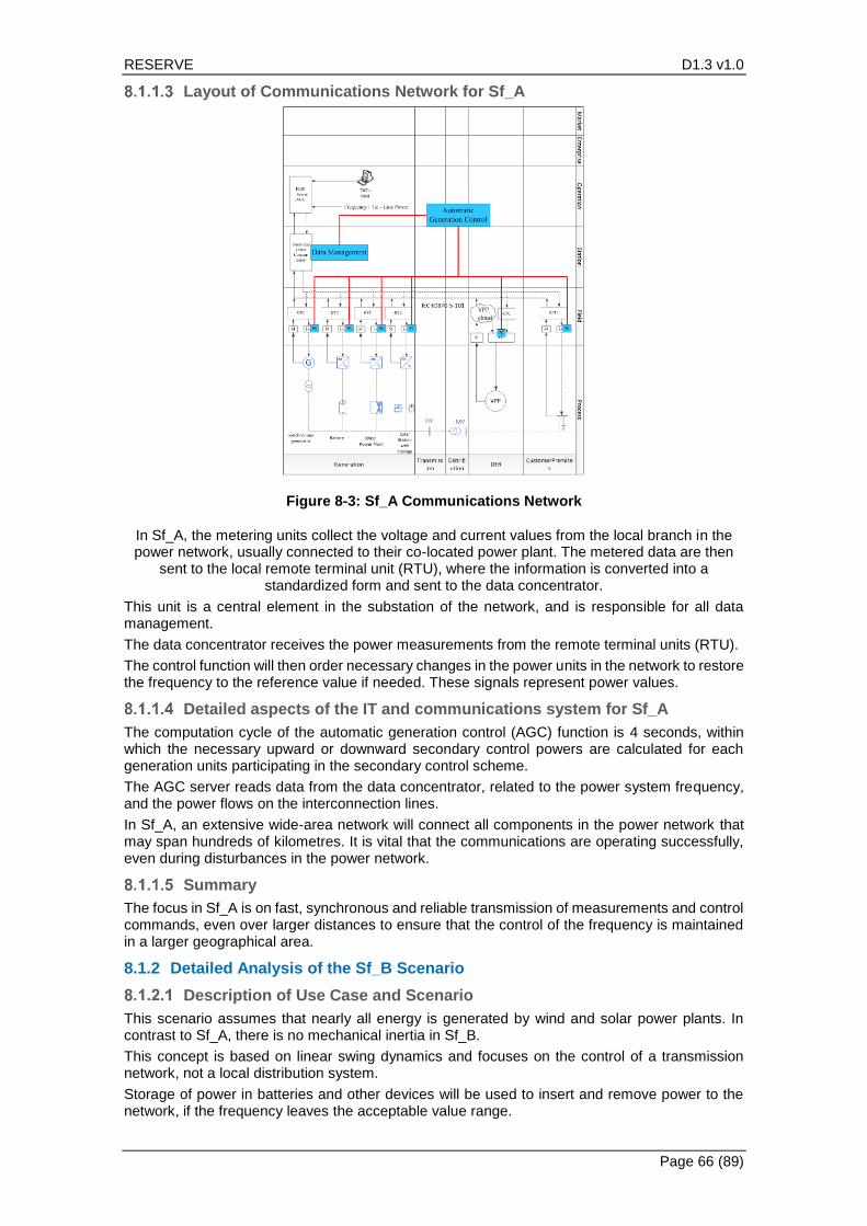
RESERVE D1.3 v1.0

(89)

Layout of Communications Network for Sf_A

Figure 8-3: Sf_A Communications Network

In Sf_A, the metering units collect the voltage and current values from the local branch in the power network, usually connected to their co-located power plant. The metered data are then

sent to the local remote terminal unit (RTU), where the information is converted into a standardized form and sent to the data concentrator.

This unit is a central element in the substation of the network, and is responsible for all data management.

The data concentrator receives the power measurements from the remote terminal units (RTU).

The control function will then order necessary changes in the power units in the network to restore the frequency to the reference value if needed. These signals represent power values.

Detailed aspects of the IT and communications system for Sf_A

The computation cycle of the automatic generation control (AGC) function is 4 seconds, within which the necessary upward or downward secondary control powers are calculated for each generation units participating in the secondary control scheme.

The AGC server reads data from the data concentrator, related to the power system frequency, and the power flows on the interconnection lines.

In Sf_A, an extensive wide-area network will connect all components in the power network that may span hundreds of kilometres. It is vital that the communications are operating successfully, even during disturbances in the power network.

Summary

The focus in Sf_A is on fast, synchronous and reliable transmission of measurements and control commands, even over larger distances to ensure that the control of the frequency is maintained in a larger geographical area.

8.1.2 Detailed Analysis of the Sf_B Scenario

Description of Use Case and Scenario

This scenario assumes that nearly all energy is generated by wind and solar power plants. In contrast to Sf_A, there is no mechanical inertia in Sf_B.

This concept is based on linear swing dynamics and focuses on the control of a transmission network, not a local distribution system.

Storage of power in batteries and other devices will be used to insert and remove power to the network, if the frequency leaves the acceptable value range.

RESERVE D1.3 v1.0

(89)

SGAM Information Layer: Business Context

As mentioned in the Sf_A section above, the purpose of the SGAM information layer is to describe the information that is being used and exchanged between power functions, power services and power components. The information objects that are exchanged between these actors are derived from the use case step description given in D1.2 section 3.4.2 “Description of Use Case and Scenario for Sf_B”.

In the SGAM framework there are two information layer elements to consider for Sf_B, the “Business Context” information layer, and the semantic understanding in the “Data Model” information layer.

Figure 8-4 is the SGAM information layer - Business Context view for 100% RES penetration. It shows the result of the mapping of the exchanged information to the power functional components of Sf_B.

Note the solid lines representing data monitoring, while the dotted lines represent control instructions being sent to controllers. See Figure 8-4: SGAM Information layer - Business Context view for 100% RES penetration, with Coordinated primary control, for an overview of the data aspects.

Figure 8-4: SGAM Information layer - Business Context view for 100% RES penetration, with Coordinated primary control

In Sf_B, power meters such as PMUs continuously measure system frequency, and send the measurements to the associated generating unit controllers and a data management system.

RESERVE D1.3 v1.0

(89)

When frequency deviation starts, RoCoF units detect the deviation and send the frequency measurements and estimates to the local controller. Local controllers respond by making the generating unit and/or storage devices inject synthetic inertia to the grid.

When disturbances occur (the frequency exceeds 20 mHz), primary control is activated to keep the frequency within the allowed range. Each controller’s primary control may or may not be coordinated.

• Case 1 – Local primary control: The controller acts on its own and adjusts the generation or consumption of the unit it is controlling, using up the operating reserve of the unit.

• Case 2 – Coordinated primary control: A centralised data management system that has being gathering the system frequency from all RTUs in the grid, calculates an amount of synthetic inertia that should be injected in to the grid by each generating unit to help stabilize the system frequency.

Secondary control (also known as AGC) is activated by the TSO or DSO within a matter of seconds to 15 minutes to replace primary control; note that today, only TSOs can do this. Secondary control corrects the frequency through an operations controller. The operations controller sends instructions to local controllers to adjust the generation from different generating units. Secondary control corrects the frequency back to the nominal value (50 Hz for Europe) and frees up the reserve generation capacities used in the primary control.

Regarding D11.1.2.3 Policy Control, given that Sf_B is covering coordinated primary control, in the case where the Sf_B data management system sends a control signal towards a controller of a generating unit and/or storage device, instructing how much synthetic inertia that should be injected in to the grid, this control signal needs to be verified against Network Codes [1] before it is sent out to the RTU.

When it comes to Network Codes, the example for Sf_B is very similar to Sf_A and can use the same Irish perspective on Network Codes as detailed by the Irish DSO [2], Irish TSO [3] and by the EU [4.

EC Article 127.1 [4] Frequency quality target parameters

The frequency quality defining parameters shall be:

(a) the nominal frequency for all synchronous areas;

(b) the standard frequency range for all synchronous areas;

(c) the maximum instantaneous frequency deviation for all synchronous areas;

(d) the maximum steady-state frequency deviation for all synchronous areas;

(e) the time to restore frequency for all synchronous areas;

(f) the time to recover frequency for the GB and IE/NI synchronous areas ;

(g) the frequency restoration range for the GB, IE/NI and Nordic synchronous

areas;

(h) the frequency recovery range for the GB and IE/NI synchronous areas; and

(i) the alert state trigger time for all synchronous areas.

EC Article 127.2. The nominal frequency shall be 50 Hz for all synchronous areas.

EC Article 127.3 The default values of the frequency quality defining parameters listed in paragraph 1 are set out in Table 1 of Annex III.

EirGrid TSO [3]: OC4.3.4.2.2 Requirements of Interconnector Frequency Response Systems:

(a) Interconnectors when Energised shall operate at all times in Frequency Control mode, unless otherwise specified by the TSO, with characteristics within the appropriate ranges as specified in Connection Conditions;

(b) The Interconnector Frequency Droop shall normally be 4% and shall be settable between 2% and 7%;

(c) No intentional time delays other than those agreed with the TSO shall be introduced into the frequency response system;

RESERVE D1.3 v1.0

(89)

(d) The Frequency Deadband shall normally be zero. Any non-zero deadband must be agreed in advance with the TSO and shall not exceed +/-15mHz.

(e) Interconnectors shall not act to control the frequency in an External System unless agreed in advance with the TSO and the External System Operator.

ESB DSO [2]: DPC4.1.1 The Frequency of supply is outside the control of the DSO however the expected standard Frequency range is as follows:

The Transmission System Frequency is nominally 50Hz:

• Normal operating range: 49.8Hz to 50.2Hz

• During system disturbances: 48.0Hz to 52.0Hz

• During exceptional system disturbances 47.0Hz to 52.0Hz

Below is a codified representation of the Network Code around frequency control, and the codified version should not contain the full text of the code. The text of the code will need to be distilled into a quantified into a temporal, numeric or categorical value so as its implementation can be simplified when used in Policy Control.

{

....

fc.rp.1 :{

eu: a127.3,

tso: OC4.3.4.2.2,

dso: DPC4.1.1

}

....

}

For example, each rule would be parsed and normalised, where possible, to have a quantifiable value, a127.3 would become

eu: {

"CE" : {

"min" : -50mHz,

"max" : +50mHz

},

"GB" : {

"min" : -200mHz,

"max" : +200mHZ

},

“IRE” : {

"min" : -200mHz,

"max" : +200mHZ

},

“Nordic” : {

"min" : -100mHz,

"max" : +100mHZ

}

}

OC4.3.4.2.2 would become:

tso : {

"min" : -15mHz,

"max" : +15mHz

}

and DPC4.1.1 would become:

dso : {

"min" : -2Hz,

"max" : +2Hz

}

The complete representation of the rule surrounding Reactive Power thresholds that must be applied to frequency control would when codified would look like this:

RESERVE D1.3 v1.0

(89)

fc.rp.1 :{

eu: {

"CE" : {

"min" : -50mHz,

"max" : +50mHz

},

"GB" : {

"min" : -200mHz,

"max" : +200mHZ

},

“IRE” : {

"min" : -200mHz,

"max" : +200mHZ

},

“Nordic” : {

"min" : -100mHz,

"max" : +100mHZ

}

},

tso : {

"min" : -15mHz,

"max" : +15mHz

},

dso : {

"min" : -2Hz,

"max" : +2Hz

}

}

This schema of the network code would allow a control signal from the data management system of Sf_B to be compared to or correlated with a policy for the system based on network codes within the each controller of the generating units.

The policy in this case would mean that no control message generated by the data management system of Sf_B would, when it’s consequences are measured, be allowed to violate the network code fc.rp.1.

SGAM Information Layer: Data Model

In the case of Sf_B for coordinated primary control, frequency data will be measured and collected at all points in the transmission network, in particular at the power generation units, and maybe all converters and inverters from the customer premises all the way to generation, will need to share data information in a common way.

It is vital that the frequency of all network elements is synchronised, otherwise the network will not have a stable frequency. If all network elements share exactly the same frequency, then the overall network will have a stable frequency too.

See Figure 8-5: SGAM Information layer – Data Model for 100% RES penetration for Sf_B for an overview of the data aspects.

RESERVE D1.3 v1.0

(89)

Figure 8-5: SGAM Information layer – Data Model for 100% RES penetration for Sf_B

As explained in the voltage control Sv_A use case, CGMES defines a set of rules which are mandatory for achieving data interoperability and for Sf_B, CGMES will be the reference data model for RE-SERVE Sf_B. Also of note given that that Romania trial site utilises data acquisition with SCADA (Supervisory Control And Data Acquisition) based on the IEC 60870-5-101 [5], then a data model based on IEC 60870-5-101 [5], will also be considered.

Layout of Communications Network

In general, the layout of the communications network for Sf_B is SCADA RTU local generator unit, where the remote terminal unit is communicating with the substation. In addition, note that RTU’s are fairly expensive devices. Therefore, the Sf_B scenario will consider other, less complex units, without the SCADA overhead, and see if they can be used. While for the moment a data management system will act as the central element running the overall monitoring and control of the transmission network regarding frequency and voltage, as well as other aspects.

RESERVE D1.3 v1.0

(89)

Detailed IT Requirements

Large number of network elements need to communicate with each other in near-real-time conditions, in order to ensure that the frequency alignment can be executed on the local, decentral level. This may involve a large number of devices, with frequent communications.

Detailed Communications Requirements

It is important that the latency for these point-to-point connections is below one second, to ensure that the measurements and corrective actions are exchanged almost in real-time. At the same time, it is essential that the communications are extremely reliable, and that no disturbances in the data exchange can be accepted. Therefore, 5G concepts such as network slicing play an important role here, as they ensure that other users of the mobile network do not affect the data traffic of the energy utility.

Summary

The Sf_B scenario puts very demanding requirements on the communications network, due to strict requirements for latency and reliability. Again, this concerns a geographically large area served by the corresponding transmission network.

8.2 Voltage Control

8.2.1 Detailed Analysis of the Sv_A Scenario

Voltage values in the grid should stay within acceptable limits in all operations of the grid, to avoid disturbances in electrical components and ensure correct transmission of energy. The goal is to keep voltage drops as small as possible (flat voltage profile). Due to the strong coupling between reactive power and voltage levels, in general, an increase of production of reactive power results in higher voltage near the production source, while an increase of consumption of reactive power results in lower voltage.

Moreover, reactive power cannot be transported over long distance due to the inductive nature of the lines (especially transmission lines). Reactive power is considered a local quantity and in the grid, there are a lot of “consumers” of reactive power and a lot of “producers” (including generators, capacitors, and FACT devices). In distribution systems with radial configuration, the voltage profile is expected to drop continuously along the lines.

With the advent of RESs connected to the grid with power electronic converters, new controllable units have appeared in the distribution grids acting as distributed generators (DGs). By taking advantage of the flexibility of the control of power electronic converters, it has been possible to develop totally distributed as well as mixed centralised-distributed automation solutions for voltage regulation.

The possible control actions include changing the position of the On-load Tap Changer (OLTC) transformers, ordering the DGs to generate/consume reactive power, and ordering DGs to curtail their real power generation or “suggesting” loads to shade their consumption.

A major challenge with these converters is to ensure small-signal voltage stability under all dynamic conditions of load vs. generation. For such a reason, a novel system automation concept has to be formulated, implemented, and validated. In this novel automation concept, all the grid-connected converters will be able to perform online identification of equivalent impedances seen at their PCC on the top of their power conversion function.

Four-Step Approach in Sv_A

While section 3.1 “Use Case Voltage Control Sv_A” in D1.2 provides detailed steps for the solution, for an understanding of the ICT requirements the process can be boiled down to four repeatable steps, with the impedance measurement being a key parameter to determine if the voltage of the grid is still enough, or corrective action is needed to maintain stability.

o Step 1: System to measure grid impedance Zg

o Step 2: System to measure output impedance Zo

o Step 3: Run online stability margin monitoring in Secondary Substation Automation Unit

o Step 4: If correction is needed, S. SAU sends desired Zo value to virtual output impedance controller which initiates corrective action (by the electronic inverter)

Step 1

The Secondary Substation (S. SAU) initiates the determination of the grid impedance.

RESERVE D1.3 v1.0

(89)

The process involves some perturbation of the grid, i.e. sending some “noise” on the local grid. Therefore, this step should not be executed more frequently than necessary.

Step 2

Using a neighbouring, second inverter, the S. SAU initiates the determination of the output impedance.

Similarly, this step involves some perturbation of the neighbour grid, i.e. sending some “noise” on the local grid. Therefore, this step should not be executed more frequently than necessary.

In this step, the perturbation is injected from Inverter 2, while the measurement is taken near Inverter 1.

Step 3

In this step, the monitoring and analysis of the local grid is executed in the S. SAU, and corrective action is initiated if necessary.

RESERVE D1.3 v1.0

(89)

If the stability margins are below their critical threshold, the SSAU will inform or alarm upper-level units such as DMS, so they can make a manual decision which inverters or loads in the system should be disconnected or connected to improve stability. The signal to turn off such network elements will be sent from the DMS directly to the selected inverters.

Step 4

If required, the S.SAU sends the desired target value for the optimum output impedance to the Virtual Output Impedance (VOI) controller. The local inverter will then take corrective actions to stabilize the local grid. The inverter will inject active or re-active power (P/Q) into the network to stabilize the voltage.

Layout of Communications Network

The chart below provides an overview of the communication flows in the Sv_A scenario.

RESERVE D1.3 v1.0

(89)

Figure 8-6: Communication Flows in the Sv_A scenario

The secondary substation automation unit (S. SAU) is the key node in this network. It initiates all types of measurements, performs the analysis of the data, and sends commands to start corrective actions.

The WSI tool, the inverter and the controller are co-located in the same unit, and share the same communication interface.

The DMS decides if an inverter is connected or disconnected from the local grid. Disconnection is the most important command here, as it can remove an inverter, and the connected end-point, from the grid completely. In that case, the S. SAU will directly communicate with the inverter of the local end-point to initiate the connection or disconnection of this unit.

8.2.2 SGAM for the Sv_A Scenario

SGAM Information Layer: Business Context for Sv_A

The purpose of the SGAM information layer is to describe the information that is being used and exchanged between power functions, power services and power components. The information objects that are exchanged between these actors are derived from the use case step description given in D1.2 section 3.1.1 “Description of Use Case and Scenario for Sv_A”.

In the SGAM framework, there are two information layer elements to consider for Sv_A the “Business Context” information layer and the semantic understanding in the “Data Model” information layer.

Please consider the image below, Figure 8-7: Sv_A Information Layer - Business Context view for Dynamic Voltage Stability Monitoring and Control. It shows the result of the mapping of the exchanged information to the power functional components of Sv_A.


RESERVE D1.3 v1.0

(89)

Figure 8-7: Sv_A Information Layer - Business Context view for Dynamic Voltage Stability Monitoring and Control

While Figure 8-8: Sv_A Information Layer - Simple Business Context view for Dynamic Voltage Stability Monitoring and Control is the full Sv_A SGAM information layer context view, the solution can be reduced to a simpler four step approach view as discussed earlier in this section.

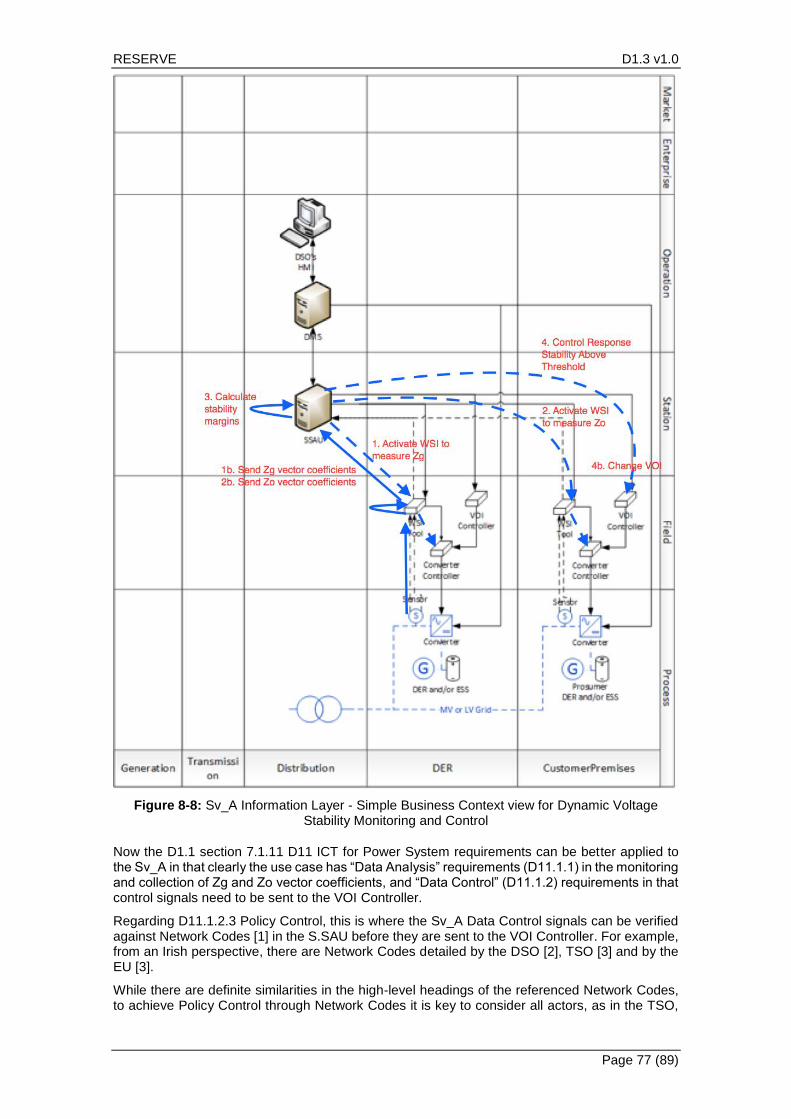
RESERVE D1.3 v1.0

(89)

Figure 8-8: Sv_A Information Layer - Simple Business Context view for Dynamic Voltage Stability Monitoring and Control

Now the D1.1 section 7.1.11 D11 ICT for Power System requirements can be better applied to the Sv_A in that clearly the use case has “Data Analysis” requirements (D11.1.1) in the monitoring and collection of Zg and Zo vector coefficients, and “Data Control” (D11.1.2) requirements in that control signals need to be sent to the VOI Controller.

Regarding D11.1.2.3 Policy Control, this is where the Sv_A Data Control signals can be verified against Network Codes [1] in the S.SAU before they are sent to the VOI Controller. For example, from an Irish perspective, there are Network Codes detailed by the DSO [2], TSO [3] and by the EU [3].

While there are definite similarities in the high-level headings of the referenced Network Codes, to achieve Policy Control through Network Codes it is key to consider all actors, as in the TSO,

RESERVE D1.3 v1.0

(89)

DSO and the EU, when developing the standard by which they are used and aggregated. One such approach would be to combine each network code under a common code heading that will encompass each actor defined network code, with each actor defined network code holding the most relevance at the level of the system that is most relevant to that actor. This will also hold the caveat of using the network code developed by the EU as a conflict resolution mechanism where a conflict occurs between the TSO and DSO instances of a specific Network Code.

The example below contains a textual representation of the same code taken from the EU commission guidelines, the ESB Networks Distribution Code (DSO) and the EirGrid Grid Code (TSO) and codified to create a common code that will encompass all three representations.

EC Article 29.1 If voltage at a connection point to the transmission system is outside the ranges defined in Tables 1 and 2 of Annex II to this Regulation, each TSO shall apply voltage control and reactive power management remedial actions in accordance with Article 22(1)(c) of this Regulation in order to restore voltages at the connection point within the ranges specified in Annex II and within time ranges specified in Article 16 of Commission Regulation No [000/2015 RfG] and Article 13 of Commission Regulation No [000/2015 DCC]. note: the ranges mentioned above are 0.90pu to 1.118pu for connection points between 110kv and 300kv stations and for connections between 300kv and 400kv the range is 0.90pu to 1.05pu.

EirGrid TSO: OC4.4.3.2: The TSO shall endeavour to maintain sufficient availability of dynamic and static reactive power in order to operate Transmission System Voltages at Connection Points within the levels specified in CC.8.3, at all times. Factors, which will influence the required Mvar capacity, include the following.

note: the levels mentioned in CC8.3 are:

(a) 400kV system: v370kV to 410kV

(b) 220kV system: 210kV to 240kV

(c) 110kV system: 105kV to 120kV.

ESB DSO: DCC11.5.2.3: For DSO type A Controllable WFPS’s irrespective of Registered Capacity and DSO type B Controllable WFPS’s with Registered Capacity ≥5MW, under steady state conditions, the Voltage Regulation System shall be capable of implementing the following Reactive Power control modes which shall be available to the DSO or TSO as agreed by DSO and TSO:

a) The Controllable WFPS shall be capable of receiving a power factor control (PF) setpoint to maintain the power factor set-point at the Connection Point;

b) The Controllable WFPS shall be capable of receiving a Reactive Power Control (Q) set-point to maintain the Reactive Power set-point at the Connection Point;

c) The Controllable WFPS shall be capable of receiving a Voltage Regulation (kV) setpoint for the voltage at the Connection Point. The Voltage Regulation System shall act to regulate the voltage at this point by continuous modulation of the Controllable WFPS’s Reactive Power output, without violating the voltage Step Emissions limits as set out in the IEC standard 61000-3-7:1996 Assessment of Emission limits for fluctuating loads in MV and HV power systems. The Controllable WFPS’s Reactive Power output shall be zero when the voltage at the Connection Point is equal to the Voltage Regulation Set-point.

d) A change to the power factor control (PF) set-point, Reactive Power control (Q) set-point, Voltage Regulation (kV) set-point or Reactive Power control mode shall be implemented by the Controllable WFPS within 20 seconds of receipt of the appropriate signal, within its Reactive Power capability range as specified in DCC11.4.5 (≥ 5MW)

e) One Reactive Power control mode shall be operational at all times with the facility to toggle between each of the Reactive Power control modes as instructed by the DSO or TSO, as agreed by the DSO and TSO. Toggling between Reactive Power controllers shall be smooth in transfer i.e. the Controllable WFPS shall calculate and implement an appropriate set-point when transferring to the new control mode. The set-point calculated for the new control mode shall be consistent with the MVAr output at that time.

Below is a codified representation of the Network Code around reactive power and voltage control, and the codified version should not contain the full text of the code. The text of the code

RESERVE D1.3 v1.0

(89)

will need to be distilled into a quantified into a temporal, numeric or categorical value so as it’s implementation can be simplified when used in Policy Control.

{

....

vc.rp.1 :{

eu: a29.1,

tso: OC4.4.3.2,

dso: DCC11.5.2.3.d

}

....

}

For example, each rule would be parsed and normalised, where possible, to have a quantifiable value, a29.1 would become

eu: {

"110-300" : {

"min" : 0.90pu,

"max" : 1.118pu

},

"300-400" : {

"min" : 0.90pu,

"max" : 1.05pu

}

}

OC4.4.3.2 would become:

tso : {

400 : {

"min" : 370,

"max" : 410

},

220 : {

"min" : 210,

"max" : 240

},

110 : {

"min" : 105,

"max" : 120

}

}

and DCC11.5.2.3 (d) would become:

dso : "≥5MW"

The complete representation of the rule surrounding Reactive Power thresholds that must be applied to Voltage control would when codified would look like this:

vc.rp.1 :{

eu: {

"110-300" : {

"min" : 0.90pu,

"max" : 1.118pu

},

"300-400" : {

"min" : 0.90pu,

"max" : 1.05pu

}

},

RESERVE D1.3 v1.0

(89)

tso : {

400 : {

"min" : 370,

"max" : 410

},

220 : {

"min" : 210,

"max" : 240

},

110 : {

"min" : 105,

"max" : 120

}

},

dso : "≥5MW"

}

This schema of the network code would allow a control signal of Sv_A to be compared to or correlated with a policy for the system based on network codes.

The policy in this case would mean that no control message generated would, when it’s consequences are measured, be allowed to violate the network code vc.rp.1.

For example, from the TSO perspective, in a 110 system a message of +30kv would bring the voltage levels outside the maximum specified in the codes and the message would not be executed. From the perspective of the DSO the only restriction that it holds is that the increase must be greater than or equal to 5MW so the control message and its effect is not in violation of the DSO section of vc.rp.1 meaning that the TSO and DSO items in the code are in conflict as the DSO version has no upper limit and the TSO version has. In instances like this the EU version of the code would be referred to and this would mean that the increase can not exceed 1.118 per unit which when calculated the increase of 30kv in a 110 system equates to 3.667pu which would confirm that the control message was in violation of the network code.

SGAM Information Layer: Data Model for Sv_A

The previous section gives an overview of data being monitored and control signals being sent for the Sv_A use case, in this section the semantic understanding of the data model and control signals being utilized for Sv_A have to be defined.

In the utility domain, there exists several data models in context with the SGAM ―Information layer. The Smart Grid JWG report [Final report of the CEN/CENELEC/ETSI Joint Working Group on Standards for Smart Grids (May 2011)] already provides a thorough overview of what has been considered state-of-the-art from the viewpoints of standardisation bodies. This report points out that CIM (IEC 61968, 61970 and 62325) and the IEC 61850 data model are the most prominent data models. The following diagram in Figure 8-9 gives some clues about the relevant areas.

RESERVE D1.3 v1.0

(89)

Figure 8-9: IEC TC 57 Seamless Integration Reference Architecture

IEC 62357 [TC57 Architecture Part 1: Reference Architecture for Power System Information Exchange] gives even better clues as to the use of XML, enterprise service buses, information exchange as should be handled in the Sv_A.

This has led to the production of a [Common Grid Model Exchange Standard (CGMES)] with specific reference on how to define the interface between ENTSO-E members’ software in order to exchange power system modelling information as required by the ENTSO-E and TSO business processes.

The [Common Grid Model Exchange Standard (CGMES) Version 2.4] is based on the following existing or expected IEC CIM standards valid for the CIM UML16v25:

IEC 61970-552: CIM XML Model Exchange Format

IEC 61970-301: Common Information Model (CIM) Base

IEC 61970-302: Common Information Model (CIM) for Dynamics Specification

IEC 61970-452: CIM Static Transmission Network Model Profiles

IEC 61970-453: Diagram Layout Profile

IEC 61970-456: Solved Power System State Profiles

IEC 61970-457: Common Information Model (CIM) for Dynamics Profile

IEC 61968-4: Application integration at electric utilities – System interfaces for distribution management - Part 4: Interfaces for records and asset management

The CGMES defines a set of rules and/or requirements which are mandatory for achieving interoperability with the CGMES, given that there are still open initiatives to harmonize the most important data models for smart grids, for Sv_A the RE-SERVE project must pick a data model standard which best suits its needs and with CGMES having created a XMI version of their model which can be loaded into the Enterprise Architect tool, which is the default tool used by all CIM modellers. Then CGMES will be the reference data model for RE-SERVE scenario Sv_A.

RESERVE D1.3 v1.0

(89)

Figure 8-10: Information - Data Model for Dynamic Voltage Stability Monitoring and Control

Also in this scenario, commands are sent to the WSI tool, and impedance vectors are monitored from the WSI Tool. Once the online stability margin monitoring tool is run on these impedance vectors, commands are sent by the S.SAU to a VOI Controller to further the stability, or to the DMS for it to make a decision on which inverters to connect/disconnect.

The format of the WSI Tool control signal commands will be based on standards IEC 61850-7-2 [11], IEC 61850-7-420 [12], and IEC 61850-8-1 [13]. The WSI Tool monitored data will be IEC 61850-8-1 (MMS) [13] and IEC 61850-9-2 (SV) [14].

RESERVE D1.3 v1.0

(89)

8.2.3 SGAM for the Sv_B Scenario

SGAM Information Layer: Business Context for Sv_B

The purpose of the SGAM information layer is to describe the information that is being used and exchanged between power functions, power services and power components for the Active Voltage Management Sv_B use case. The information objects that are exchanged between these actors are derived from the use case step description given in D1.2 section 3.2.1 “Description of Use Case and Scenario for Sv_B”.

In the SGAM framework there are two information layer elements to consider for Sv_B the “Business Context” information layer and the semantic understanding in the “Data Model” information layer.

Please consider Figure 8-11: Information Layer – Business Context view for Active Voltage Management below. It shows the result of the mapping of the exchanged information to the power functional components of Sv_B.


Figure 8-11: Information Layer – Business Context view for Active Voltage Management

RESERVE D1.3 v1.0

(89)

Synchronized measurements and control signals are vital for the success and validation of the Active Voltage Management use case Sv_B in a field trial environment. Although it should be noted that the time scale envisioned for the voltage regulation is of the order of minutes.

For Sv_B, the types of state variable data being collected includes:

• Three-phase voltage magnitude measurement as measured at the DER and customer premise locations.

• The reactive power as measured at the DER and customer premise locations.

At the secondary sub-station (S.SAU) the measurements will be logged and time-stamped, including the voltage phase and angle, and the current flow through the feeder.

Given that the S.SAU has the full picture of all the RES on the feeder line from the substation, the S.SAU can calculate a desirable set point for the active power and reactive power for a RES in the future to ascertain a volt-VAr curve that will be maintain voltage stability at that future point. This calculation is based on a predetermined multi period AC OPF formulation of the surrounding network.

The S.SAU will send as a control signal the desirable set point for the active power (P) and reactive power (Q) to the RTU controller connected to the RES.

Now the D1.1 section 7.1.11 D11 ICT for Power System requirements can be better applied to the Sv_B, as the use case has “Data Analysis” requirements (D11.1.1) in the monitoring and collection of the three-phase voltages and currents from the DER/Customer premises. “Data Control” (D11.1.2) requirements are required in that control signals for active power (P) and reactive power (Q) to the RTU controller connected to the RES.

In regard to D11.1.2.3 Policy Control, this is where the Sv_B S.SAU control signal for the active power (P) and reactive power (Q) needs to be verified against Network Codes [1] in the S.SAU before they are sent to the RTU of the RES. For example, from an Irish perspective there are Network Codes detailed by the DSO [2], TSO [3] and by the EU [4].

The example below contains a textual representation of the same Voltage Control code taken from the EU commission guidelines, the ESB Networks Distribution Code (DSO) and the EirGrid Grid Code (TSO) and codified to create a common code that will encompass all three representations.

It should be noted that currently there are no suitable codes defined in the context of RES at the LV level of the grid and there is the potential that a local RES installation would fall short in capacity, required to comply with the network codes in their current form. However, with this implementation and codification of the network codes, a standard process is in place for when new codes are developed, and essentially can be implemented in the same way as the existing ones.

The demonstration of the codification of the network codes below is based on the EU Commission guidelines on Voltage Control and Reactive power management.

EC Article 27.1 in association with Article 18 states that each TSO shall endeavour to ensure that during the normal state the voltage remains in steady-state at the connection points of the transmission system within the ranges specified in the Tables 1 and 2 of Annex II.

Table 8-1: Voltage ranges at the connection point between 110 kV and 300 kV

Synchronous Area Voltage range

Continental Europe 0.90pu - 1.118pu

Nordic 0.90pu - 1.05pu

Great Britain 0.90pu - 1.10pu

Ireland and Northern Ireland 0.90pu - 1.118pu

Baltic 0.90pu - 1.118pu

RESERVE D1.3 v1.0

(89)

Table 8-2: Voltage ranges at the connection point between 300 kV and 400 kV

Synchronous Area Voltage range

Continental Europe 0.90pu - 1.05pu

Nordic 0.90pu - 1.05pu

Great Britain 0.90pu - 1.05pu

Ireland and Northern Ireland 0.90pu - 1.05pu

Baltic 0.90pu - 1.097pu

EirGrid (TSO): CC8.3.2 During Transmission System disturbances or following transmission faults:

(a) 400kV system: 350kV to 420kV;

(b) 220kV system: 200kV to 245kV;

(c) 110kV system: 99kV to 123kV.

Some Transmission System disturbances (e.g. earth faults, lightning strikes) will result in short-term Voltage deviations outside the above ranges.

ESB Networks (DSO): DPC4.2.2d The DSO shall operate the Distribution System so as ensure that the voltage at the supply terminals, as defined in EN 50160, complies with that standard. The Low Voltage range tolerance shall be 230V +/- 10%. The resulting voltage at different points on the system depends on several factors, but at the Connection Point with Customers can be expected to be in accordance with Table 2 under steady state and normal operating conditions.

Table 8-3: Operating Voltage Range

Nominal Voltage Highest Voltage Lowest Voltage

230V 253V 207V

400V 440V 360V

10kV 11.1kV Variable according to operating conditions.

Information on particular location

on request by the User concerned 20kV 22.1kV

38kV 43kV

110kV 120kV

Higher maximum voltages can arise at the Connection Point with Generators as per Table 5 in clause DCC10.5.

Table 8-4: Maximum Voltage at Connection Point with Generators

Nominal Voltage Highest Voltage

230V 253V

400V 440V

10kV 11.3kV

20kV 22.5kV

38kV 43.8kV

110kV 120kV

RESERVE D1.3 v1.0

(89)

Below is a codified representation of the Network Code around reactive power and voltage control, and the codified version.

{

....

vc.rpm.1 :{

eu: a27.1,

tso: CC8.3.2,

dso: DPC4.2.2

}

....

}

The text of the code will need to be distilled into a quantified into a temporal, numeric or categorical value so as it’s implementation can be simplified when used in a live scenario. For example, each rule would be parsed and normalised, where possible, to have a quantifiable value, a27.1 would become

eu: {

"110-300" : {

"min" : 0.90pu,

"max" : 1.118pu

},

"300-400" : {

"min" : 0.90pu,

"max" : 1.05pu

}

}

CC8.3.2 would become:

tso : {

400 : {

"min" : 370,

"max" : 410

},

220 : {

"min" : 200,

"max" : 245

},

110 : {

"min" : 99,

"max" : 123

}

}

and DPC4.2.2 (d) would become:

dso : {

400 : {

"min" : 360,

"max" : 440

},

230 : {

"min" : 207,

"max" : 253

},

110 : {

"max" : 120

},

38 : {

"max" : 43

RESERVE D1.3 v1.0

(89)

},

20 : {

"max" : 22.1

},

10 : {

"max" : 11.1

}

}

The complete representation of the rule surrounding Reactive Power Management thresholds that must be applied to Voltage control would when codified would look like this:

vc.rpm.1 :{

eu: {

"110-300" : {

"min" : 0.90pu,

"max" : 1.118pu

},

"300-400" : {

"min" : 0.90pu,

"max" : 1.05pu

}

},

tso : {

400 : {

"min" : 370,

"max" : 410

},

220 : {

"min" : 200,

"max" : 245

},

110 : {

"min" : 99,

"max" : 123

}

},

dso : {

400 : {

"min" : 360,

"max" : 440

},

230 : {

"min" : 207,

"max" : 253

},

110 : {

"max" : 120

},

38 : {

"max" : 43

},

20 : {

"max" : 22.1

},

10 : {

"max" : 11.1

}

}

}

This normalised, codified schema of the network code would allow a reading or a control message to be compared to or correlated with a policy to control the system. The policy in this case would

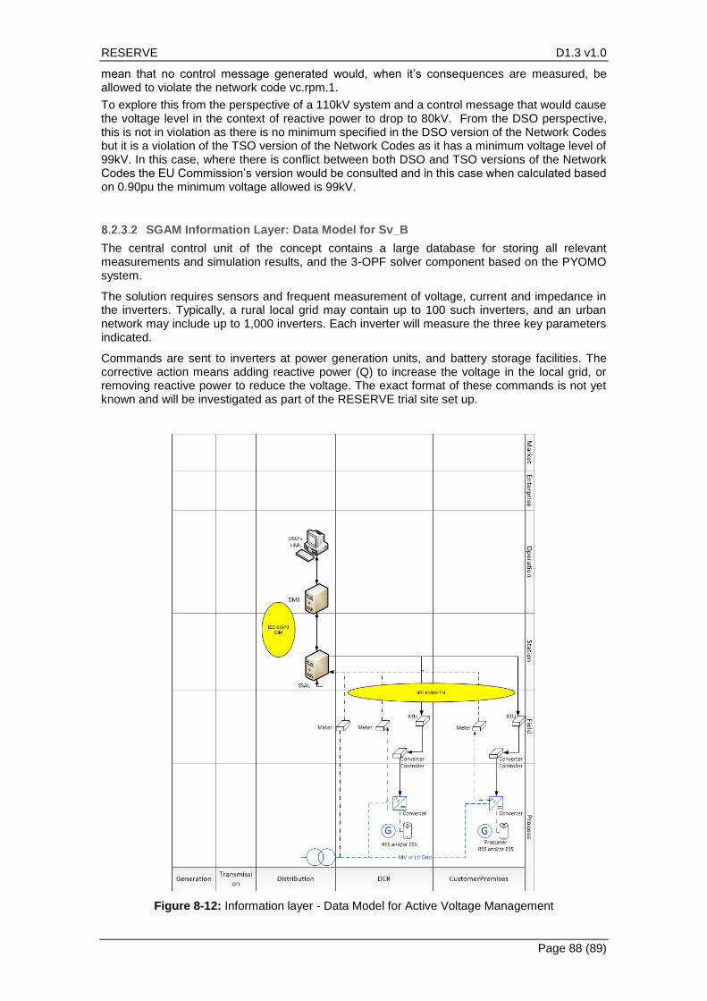
RESERVE D1.3 v1.0

(89)

mean that no control message generated would, when it’s consequences are measured, be allowed to violate the network code vc.rpm.1.

To explore this from the perspective of a 110kV system and a control message that would cause the voltage level in the context of reactive power to drop to 80kV. From the DSO perspective, this is not in violation as there is no minimum specified in the DSO version of the Network Codes but it is a violation of the TSO version of the Network Codes as it has a minimum voltage level of 99kV. In this case, where there is conflict between both DSO and TSO versions of the Network Codes the EU Commission’s version would be consulted and in this case when calculated based on 0.90pu the minimum voltage allowed is 99kV.

SGAM Information Layer: Data Model for Sv_B

The central control unit of the concept contains a large database for storing all relevant measurements and simulation results, and the 3-OPF solver component based on the PYOMO system.

The solution requires sensors and frequent measurement of voltage, current and impedance in the inverters. Typically, a rural local grid may contain up to 100 such inverters, and an urban network may include up to 1,000 inverters. Each inverter will measure the three key parameters indicated.

Commands are sent to inverters at power generation units, and battery storage facilities. The corrective action means adding reactive power (Q) to increase the voltage in the local grid, or removing reactive power to reduce the voltage. The exact format of these commands is not yet known and will be investigated as part of the RESERVE trial site set up.

Figure 8-12: Information layer - Data Model for Active Voltage Management

RESERVE D1.3 v1.0

(89)

As explained in the Sv_A use case, CGMES defines a set of rules and/or requirements which are mandatory for achieving data interoperability and for Sv_B, CGMES will be the reference data model for RE-SERVE Sv_B.

In addition, as indicated by the Sv_A use case, the format of the corrective action control signal commands will be based on standards IEC 61850-7-2 [6] and IEC 61850-8-1 [8]. The DES/Customer Premise monitored data format will be based IEC 61850-8-1 (MMS) [8] and IEC 61850-9-2 (SV) [9].

RESERVE D1.3 v1 D1.3 v1.0 Page 3 (89) Authors Partner Name Phone/ e-mail EDD Steffen Bretzke Phone:...

Documents

Transcript of RESERVE D1.3 v1 D1.3 v1.0 Page 3 (89) Authors Partner Name Phone/ e-mail EDD Steffen Bretzke Phone:...