Research Article Longitudinal/Lateral Stability...
16
Research Article Longitudinal/Lateral Stability Analysis of Vehicle Motion in the Nonlinear Region Keji Chen, 1 Xiaofei Pei, 1 Guocheng Ma, 2 and Xuexun Guo 3 1 Hubei Key Laboratory of Advanced Technology of Automotive Components, Wuhan 430070, China 2 School of Mechanical & Engineering, Beijing Institute of Technology, Beijing 100081, China 3 Hubei Collaborative Innovation Center of Automotive Components Technology, Wuhan 430070, China Correspondence should be addressed to Xiaofei Pei; [email protected] Received 5 April 2016; Revised 16 June 2016; Accepted 10 July 2016 Academic Editor: Yan-Jun Liu Copyright © 2016 Keji Chen et al. is is an open access article distributed under the Creative Commons Attribution License, which permits unrestricted use, distribution, and reproduction in any medium, provided the original work is properly cited. We focus on the study of motion stability of vehicle nonlinear dynamics. e dynamic model combining with Burckhardt tire model is firstly derived. By phase portrait method, the vehicle stability differences of three cases, front wheels steering/four-wheel steering case, front/rear/four-wheel braking case, and high/low road friction case, are characterized. With the Jacobian matrix, the stable equilibrium point is found and stable areas are calculated out. Similarly, the stability boundaries corresponding to different working conditions are also captured. With vehicle braking or accelerating in the steering process, the relationship between front/rear wheel slippage and the stable area is examined. Comparing with current literatures, the research method and its results present the novelty and provide a guideline for new vehicle controller design. 1. Introduction Towards the developing trend of intelligent vehicle, ADAS (advanced driver assistant system) and active safety technol- ogy have drawn attention in recent years. Like Ford motor, it proposed a vehicle handling limit warning system based on VSC (vehicle stability control) for the next generation of accident-free vehicle [1]. Currently, the intelligent control system has been designed to handle transient unstable vehicle motion in a guaranteed-safety range. However, the study on the vehicle handling performance, as an essential aspect in vehicle nonlinear dynamics, is never out of date, and a deep insight into the dynamics will bring benefits for advanced controller design. Facing the challenge of nonlinear system with uncertain dynamic, many intelligent control algorithms such as adap- tive fuzzy control and dynamic programming approach are introduced [2–8]. Fuzzy adaptive optimal control was adopted for nonlinear discrete-time systems with dead-zone in [5] and fuzzy adaptive inverse compensation method was used for tracking control of unknown nonlinear system in [6]. Furthermore, [7] outlined a fuzzy adaptive cruise control system which could dynamically adjust the speed of vehicle in accordance with the speed limit of the road. For trajectory tracking problem of mobile robot, [8] presented a model predictive control incorporating neural-dynamic optimiza- tion. Instead of optimizing the control algorithm, we focus on the fundamental of vehicle motion stability for controller designing. With nonlinear properties of the coupled tire forces taken into account, vehicle lateral stability would be affected when longitudinal dynamics is under control. Especially during emergencies, steering behavior with hard brake easily leads the vehicle to driſt. It is also known that increasing tire slip ratio reduces the stable region of the vehicle dynamics. Most existing lateral controllers such as VSC and AFS (active front steering) is based on the assumption that wheel slip angle is less than 4 deg [9–11]. For these controllers, only linear properties of tire lateral forces are taken into account. And for longitudinal slip controllers such as ABS and TCS, tire force Hindawi Publishing Corporation Mathematical Problems in Engineering Volume 2016, Article ID 3419108, 15 pages http://dx.doi.org/10.1155/2016/3419108
Transcript of Research Article Longitudinal/Lateral Stability...

Research ArticleLongitudinalLateral Stability Analysis of VehicleMotion in the Nonlinear Region
Keji Chen1 Xiaofei Pei1 Guocheng Ma2 and Xuexun Guo3
1Hubei Key Laboratory of Advanced Technology of Automotive Components Wuhan 430070 China2School of Mechanical amp Engineering Beijing Institute of Technology Beijing 100081 China3Hubei Collaborative Innovation Center of Automotive Components Technology Wuhan 430070 China
Correspondence should be addressed to Xiaofei Pei peixiaofei7whuteducn
Received 5 April 2016 Revised 16 June 2016 Accepted 10 July 2016
Academic Editor Yan-Jun Liu
Copyright copy 2016 Keji Chen et al This is an open access article distributed under the Creative Commons Attribution Licensewhich permits unrestricted use distribution and reproduction in any medium provided the original work is properly cited
We focus on the study ofmotion stability of vehicle nonlinear dynamicsThe dynamicmodel combiningwith Burckhardt tiremodelis firstly derived By phase portrait method the vehicle stability differences of three cases front wheels steeringfour-wheel steeringcase frontrearfour-wheel braking case and highlow road friction case are characterized With the Jacobian matrix the stableequilibrium point is found and stable areas are calculated out Similarly the stability boundaries corresponding to different workingconditions are also capturedWith vehicle braking or accelerating in the steering process the relationship between frontrear wheelslippage and the stable area is examined Comparing with current literatures the researchmethod and its results present the noveltyand provide a guideline for new vehicle controller design
1 Introduction
Towards the developing trend of intelligent vehicle ADAS(advanced driver assistant system) and active safety technol-ogy have drawn attention in recent years Like Ford motorit proposed a vehicle handling limit warning system basedon VSC (vehicle stability control) for the next generationof accident-free vehicle [1] Currently the intelligent controlsystem has been designed to handle transient unstable vehiclemotion in a guaranteed-safety range However the study onthe vehicle handling performance as an essential aspect invehicle nonlinear dynamics is never out of date and a deepinsight into the dynamics will bring benefits for advancedcontroller design
Facing the challenge of nonlinear system with uncertaindynamic many intelligent control algorithms such as adap-tive fuzzy control and dynamic programming approachare introduced [2ndash8] Fuzzy adaptive optimal control wasadopted for nonlinear discrete-time systems with dead-zonein [5] and fuzzy adaptive inverse compensation method was
used for tracking control of unknown nonlinear system in[6] Furthermore [7] outlined a fuzzy adaptive cruise controlsystem which could dynamically adjust the speed of vehiclein accordance with the speed limit of the road For trajectorytracking problem of mobile robot [8] presented a modelpredictive control incorporating neural-dynamic optimiza-tion Instead of optimizing the control algorithm we focuson the fundamental of vehicle motion stability for controllerdesigning
With nonlinear properties of the coupled tire forces takeninto account vehicle lateral stability would be affected whenlongitudinal dynamics is under control Especially duringemergencies steering behavior with hard brake easily leadsthe vehicle to drift It is also known that increasing tire slipratio reduces the stable region of the vehicle dynamics Mostexisting lateral controllers such as VSC and AFS (active frontsteering) is based on the assumption that wheel slip angleis less than 4 deg [9ndash11] For these controllers only linearproperties of tire lateral forces are taken into account And forlongitudinal slip controllers such as ABS and TCS tire force
Hindawi Publishing CorporationMathematical Problems in EngineeringVolume 2016 Article ID 3419108 15 pageshttpdxdoiorg10115520163419108
2 Mathematical Problems in Engineering
is also restricted in the unsaturated zone As the tire dynamicsis not beyond linear characteristics ultimate capability ofvehicle on slippery road or at high speed is hard to reachNowadays the ICC (integrated chassis control) system hasbecome a research focus because ICC could enable VSC AFSand other chassis controllers to work cooperatively to copewith tire nonlinearities [12ndash14]
In the design of linear controller the linearized modelcould be used to represent nonlinear system in the neigh-borhood of equilibria Nonlinear vehicle system generally hasmore than one equilibrium point Besides vehicle dynam-ics are often parameter-dependent Therefore a compre-hensive understanding of motion stability will provide theknowledge for advanced vehicle dynamic controllers Phaseportrait is a useful method for analysis of vehicle stableregion Reference [15] was the first to propose phase portraitmethod to describe the variation of sideslip angle and yawrate in critical motion situation Thereafter a saddle-nodebifurcation was found with phase portrait method [16] Itwas shown that vehicle steering system has one stable andtwo unstable equilibria Reference [17] reported bifurcationphenomenonunder purely brakingmaneuvers Furthermorea hopf bifurcation was discovered when 4WS (four-wheelsteering) is applied in typical road conditions [18] But thisanalytical method is complicated for real time controllerReference [19] introduced a geometric method The vehiclehandling characteristic and equilibria for sharply corneringmaneuver is given by joint-point locus geometry In additionthe lateral stability analyses in [20ndash22] indicated that thestable equilibrium point disappears when the vehicle speedand steering angle increase over a certain limit Howeverthe work in [18ndash22] assumed the constant velocity and zerotire slip ratio and the effect of the tire slip ratio on lateralvehicle stability was ignored Therefore we provide a novelstability analysis for transient vehicle motion on variousrunning conditions by considering the coupling betweenlongitudinal and lateral tire force The result can be appliedto active control design such as the next generation of VSCor ADAS systems It will help the controller find the stableregion of vehicle motion especially in critical situations Fur-thermore with the guideline the vehicle can conduct someaggressive maneuvers that are unstable seemingly but safeactually
The estimation of tireroad friction forces is an importantaspect in vehicle dynamic studies References [23ndash25] pro-posed many dynamic-based tire models Since Burckhardttire model could describe the characteristic of coupled tireforce with simple structure [26] its exponential form is moresuitable for the large amount of calculation in this paper Ifa more precise tire model is used here the conclusion willbe consistent with our analysis but with a more complexprocedure and expression
This paper is organized as follows a vehicle dynamicmodel and tire model are firstly presented in Section 2followed by a primary stability analysis for vehicle lateralmotion and coupled longitudinallateral motion in Section 3We then discuss vehicle stable region on various tire slipconditions in Section 4 before concluding the paper inSection 5
lr lf
120596
Fyr
Fxr
120575ry
x
120590
Fyf Fxf
120575f
Figure 1 Vehicle dynamic model
2 Vehicle Dynamics Models
Any analysis for vehicle motion is based on dynamic modelHere a classic bicyclemodel is used for 4WSvehicle as shownin Figure 1 with the following assumptions
(1) The origin of 119909119910-coordination is fixed at the vehiclersquosmass center
(2) Only vehicle planar motion is considered and rollpitch vertical motion are ignored
(3) Steering angles applied to left and right wheels aretreated to be equal
(4) Front track is assumed to be the same as rear track
In bicycle model front and rear wheel respectivelyrepresent the resultant force of left and right wheels Besidesan additional torque 119872eq is applied in yaw moment thatresults from the difference of the tire forces Ignoring theair drag and tire rolling resistance the vehicle dynamicequationsincluding longitudinal lateral and yaw motionsare given in (1) to (3)
119898(V119909minus V119910120596) = 119865
119909119891cos 120575119891minus 119865119910119891
sin 120575119891+ 119865119909119903cos 120575119903
minus 119865119910119903sin 120575119903
(1)
119898(V119910+ V119909120596) = 119865
119909119891sin 120575119891+ 119865119910119891
cos 120575119891+ 119865119909119903sin 120575119903
+ 119865119910119903cos 120575119903
(2)
119868119911 = 119865
119909119891sin 120575119891119897119891+ 119865119910119891
cos 120575119891119897119891
minus (119865119909119903sin 120575119903119897119903+ 119865119910119903cos 120575119903119897119903)
+119872eq
(3)
where 119898 is vehicle mass V119909is longitudinal velocity V
119910is
lateral velocity120596 is vehicle yaw rate119865119909119891
and119865119909119903 respectively
represent longitudinal forces of the front and rear tire 119865119910119891
and 119865119910119903 respectively represent tire lateral forces 120575
119891and 120575
119903
respectively represent wheels steering angles 119868119911is the yaw
moment of vehicle inertia 119897119891and 119897119903are the distances from
vehicle mass center to the front and rear axles
Mathematical Problems in Engineering 3
Table 1 Burckhardt model values
Friction 1198961
1198962
1198963
1198961199091
1198961199092
1198961199093
1198961199101
1198961199102
1198961199103
High-mu minus0726 03235 4625 0884 minus2612 minus0131 0855 minus2404 minus0155
Low-mu minus0716 3642 19889 0185 minus255 minus0052 0193 minus224 minus0046
As Burckhardt tire model is used in the paper the tireforce can be given in
119865119909(119904 120572) = 119865
119911(1198961|tan (120572)| + 1)
sdot [sgn (119904) 1198961199091
(1 minus 119890sgn(119904)119896
1199092sdot119904
) + 1198961199093
sdot 119904]
119865119910(119904 120572) = minus119865
119911(
1198962|119904| + 1
1198963|119904| + 1
)
sdot [sgn (tan (120572)) 1198961199101
(1 minus 119890sgn(tan(120572))119896
1199102sdottan(120572)
) + 1198961199103
sdot tan (120572)]
(4)
where 119865119909 119865119910 and 119865
119911denote longitudinal force lateral force
and normal force respectively 119904 is longitudinal slip ratio 120572 issideslip angle sgn(sdot) is the sign function 119896
1 1198962 1198963 1198961199091 1198961199092
1198961199093 1198961199101 1198961199102 and 119896
1199103are all model parameters and the values
are given for highlow-mu road surface in Table 1The front and rear tireroad friction coefficients are
defined as follows
120583119891119903
= (1198961
10038161003816100381610038161003816tan (120572
119891119903)
10038161003816100381610038161003816+ 1)
sdot [sgn (119904119891119903) 1198961199091
(1 minus 119890sgn(119904119891119903)1198961199092sdot119904119891119903
) + 1198961199093
sdot 119904119891119903]
120578119891119903
= minus(
1198962
10038161003816100381610038161003816119904119891119903
10038161003816100381610038161003816+ 1
1198963
10038161003816100381610038161003816119904119891119903
10038161003816100381610038161003816+ 1
)
sdot [sgn (tan (120572119891119903)) 1198961199101
(1 minus 119890sgn(tan(120572
119891119903))1198961199102sdottan(120572
119891119903)
)
+ 1198961199103
sdot tan (120572119891119903)]
(5)
Therefore 119865119909119891119903
and 119865119910119891119903
can be expressed as
119865119909119891119903
= 119865119911119891119903
sdot 120583119891119903
119865119910119891119903
= 119865119911119891119903
sdot 120578119891119903
(6)
When vehicle brakes hard the longitudinal load transfercannot be neglected The loads of front and rear tire could begiven by
119865119911119891
=
119897119903
119897119891+ 119897119903
119898119892 minus
ℎ
119897119891+ 119897119903
(119865119911119891120583119891cos 120575119891
minus 119865119911119891120578119891sin 120575119891+ 119865119911119903120583119903cos 120575119903minus 119865119911119903120578119903sin 120575119903)
119865119911119903
=
119897119891
119897119891+ 119897119903
119898119892 minus
ℎ
119897119891+ 119897119903
(119865119911119891120583119891cos 120575119891minus 119865119911119891120578119891sin 120575119891
+ 119865119911119903120583119903cos 120575119903minus 119865119911119903120578119903sin 120575119903)
(7)
where ℎ is the height of vehicle mass center
By transformation the load transfer coefficients aredefined as
120577119891=
119897119903minus 119875119903
119871 + 119875119891minus 119875119903
120577119903=
119897119891+ 119875119891
119871 + 119875119891minus 119875119903
(8)
where 119875119891
= (119906119891cos 120575119891
minus 120578119891sin 120575119891)ℎ 119875119903
= (119906119903cos 120575119903minus
120578119903sin 120575119903)ℎ
Therefore 119865119911119891119903
can be given in
119865119911119891119903
= 119898119892120577119891119903 (9)
Due to differences of left and right tire forces the extratorque119872eq can be expressed as
119872eq = Δ119865119911119891120578119891119861 sin 120575
119891minus Δ119865119911119891120583119891119861 cos 120575
119891
+ Δ119865119911119903120578119903119861 sin 120575
119903minus Δ119865119911119903120583119903119861 cos 120575
119903
(10)
where119861 is the half wheel trackΔ119865119911119891andΔ119865
119911119903are the normal
force differences between left and right tire which can beexpressed as follows
Δ119865119911119891119903
= Δ119865119911120577119891119903
= minus
ℎ
119861
(119865119909119891
sin 120575119891+ 119865119910119891
cos 120575119891
+ 119865119909119903sin 120575119903+ 119865119910119903cos 120575119903) 120577119891119903
(11)
Let 120590 denote the tangent value of vehicle sideslip anglenamely 120590 = V
119910V119909 Then the sideslip angles of front and rear
tire can be expressed as follows
120572119891= arctan(120590 +
119897119891120596
V119909
) minus 120575119891
120572119903= arctan(120590 minus
119897119903120596
V119909
) minus 120575119903
(12)
Besides the lateral velocity in (2) can be derived accord-ing to kinematic relations
V119910= V119909+ V119909120590 (13)
Then taking 120590 and 120596 as state variables the governingequations for vehicle planarmotion at a certain instantaneousV119909 120575119891119903 and 119904
119891119903could be expressed as follows
=
119892
V119909
(120577119891119876119891+
120590
ℎ
120577119891119875119891+ 120577119903119876119903+
120590
ℎ
120577119903119875119903) minus 120596 (120590
2
+ 1)
(14)
=
119898119892
119868119911
[(119897119891120577119891119876119891minus 119897119903120577119903119876119903)
+ (120577119891119875119891+ 120577119903119875119903) (120577119891119876119891+ 120577119903119876119903)]
(15)
4 Mathematical Problems in Engineering
Table 2 Vehicle model values
119898 (kg) 119868119911(kgsdotm2) ℎ (m) 119897
119891(m) 119897
119903(m) 119861 (m)
1295 1580 0469 0946 1526 0715
where 119876119891= 120583119891sin 120575119891+ 120578119891cos 120575119891 119876119903= 120583119903sin 120575119903+ 120578119903cos 120575119903
And all related parameters values are shown in Table 2
3 Vehicle Stability CharacteristicAnalysis by Phase Portrait
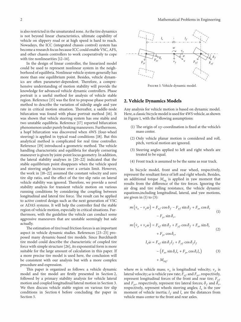
In this section vehicle stability analysis is discussed by usingphase portrait method The phase portraits are obtained bynumerically solving (14) and (15) with Runge-Kutta methodunder series of initial states of vehicle motion In all thephase portraits ldquotimesrdquo denotes an initial vehicle state andthe corresponding curve denotes the locus of the vehiclemotion states Additionally we define attraction domain ofthe nonlinear dynamical systems as the stable region atthe given vehicle motion and input The vehicle motion isconsidered to be stable when vehiclemotion states are locatedwithin the stable region
31 Stability Analysis for Pure Steering In this part we extendthe lateral stability analyses in [18ndash22] More comprehensiveoperating conditions (eg highlow friction road and 4WScontrol) are taken into account We use the phase portraitmethod to analyze vehicle motion stability under steeringaction The result also provides a foundation for furthercomparison with braking and steering in latter part
Figure 2 illustrates 120596-120590 dynamical characteristics withsteering angle 120575
119891= 002 rad and 120575
119903= 0 rad respectively
We observe that the stable region becomes narrower withincreasing velocity V
119909when the vehicle corners Figures 2(b)
and 2(d) show that the vehicle fails to maintain a steady stateat 35ms on high-mu road surface or 15ms on low frictionroad as there is no stable region in the phase portraitsTherefore the front wheels steering maneuver is forbiddenwhen vehicle exceeds a critical speed
Figure 3 shows the 120596-120590 phase portraits under the changeof steering angle 120575
119891 We observe the following facts from this
plot
(1) Increasing steering angle 120575119891will reduce the stable
region(2) The stable equilibrium point disappears at a critical
steering angle 120575119891 such as 008 rad in Figure 3(c) and
002 rad in Figure 3(f)(3) The stable equilibrium point is at the origin when
120575119891
= 0 rad For nonzero steering angle the stableequilibrium point is no longer fixed at the origin
It can be summarized from Figures 2 and 3 that whethervelocity V
119909or steering angle 120575
119891increases the stable equilib-
rium point will move to the unstable saddle point Further-more the stable equilibrium point will merge with one of theunstable saddle equilibria at certain condition Then there isno stable region
Besides the 120596-120590 phase portraits are compared betweenhigh-mu friction and low-mu friction conditions For high-mu road surface the stable region is much larger and is morerobust to the change of the vehicle velocity and steering angleWhile for low-mu road surface a slight steering maneuvercould easily make the vehicle unstable (see Figures 3(d) 3(e)and 3(f))
A similar stability analysis is given for 4WS vehicle inFigures 4 and 5The rear wheels steering is taken into accountto compensate the oversteer of the front wheels Here acompliance steering strategy is adopted for 4WS controlwhich is mathematically expressed as
120575119903= 119870120575119891 (16)
where119870 is a parameter that represents the linear relationshipbetween 120575
119891and 120575119903
Without losing generality119870 is set to 05 in Figures 4 and 5Although the two phase portraits look similar to those shownin Figures 2 and 3 we can observe that the risk of instability isreduced by the rearwheels steeringUnder the same V
119909and 120575119891
conditions 2WS (front wheels steering) vehicle cannot keepstable motion in Figures 2(b) 2(d) 3(c) and 3(f) but 4WSvehicle is still in safe area as showed by Figures 4(a) 4(b) 5(a)and 5(b)
32 Stability Analysis for Steering and Braking A properbraking maneuver could increase the understeer tendencywhen vehicle is in high speed cornering such as the principleof VSC On the contrary applying a rude brake will deteri-orate the vehicle stability severely In this part we analyzethe coupled longitudinal and lateral stability under variousvehicle operation conditions
Figures 6 and 7 illustrate the phase portraits of vehicleplanar motion for 2WS and 4WS respectively As seen inFigures 6(a) 6(d) 7(a) and 7(d) the stable region expandswhen applying brake force on front wheels Similar to 4WScontrol front wheels braking can increase the tendency ofundersteer for 2WS vehicle Figures 6(b) 6(e) 7(b) and 7(e)show that rear wheels braking totally destruct the formationof stable region even for 4WS vehicle on high-mu roadsurface In other words the vehicle will lose its stabilityimmediately at any initial condition if only the rear wheelsbrake during cornering This situation is dangerous andshould be avoided When the four-wheel braking is appliedwe can find the stability of 2WS vehicle is improved bycomparing Figures 6(c) and 6(f) with Figures 3(c) and 3(f)but the stability of 4WS vehicle worsens comparing Figures7(c) and 7(f) with Figures 5(b) and 5(d) Therefore four-wheel braking is only useful for 2WS vehicle in some cases
4 Vehicle Stability Boundary Analysis byJacobian Matrix
In this section we further figure out the stability boundaryaccording to various steering braking or road frictionconditions As is analyzed above the structures of phaseportraits change with specific operation conditions Whenthe stable equilibrium point merges with the unstable saddle
Mathematical Problems in Engineering 5
minus05minus1 050 1120590
minus2
minus15
minus1
minus05
0
05
1
15
2120596(rads)
(a) V119909= 25ms
minus05minus1 050 1120590
minus2
minus15
minus1
minus05
0
05
1
15
2
120596(rads)
(b) V119909= 35ms
minus05minus1 050 1120590
minus2
minus15
minus1
minus05
0
05
1
15
2
120596(rads)
(c) V119909= 10ms
minus05minus1 050 1120590
minus2
minus15
minus1
minus05
0
05
1
15
2
120596(rads)
(d) V119909= 15ms
Figure 2 Phase portraits for 120575119891= 002 rad and 120575
119903= 0 rad (a) and (b) On high friction road (c) and (d) on low friction road
point there is no stable region in the phase plane We assumethat if a stable equilibrium point exists the correspondingvehicle motion is stable Therefore we could determinevehicle motion stability by the eigenvalues of the Jacobianmatrix at each equilibrium point Let119891
1denote the transform
of (15) and let 1198912denote the transform of (16) the Jacobian
matrix J is given as
J = 120597f120597x
=
[
[
[
[
1205971198911
1205971199091
1205971198911
1205971199092
1205971198912
1205971199091
1205971198912
1205971199092
]
]
]
]
(17)
where
1205971198911
1205971199091
=
119892
V119909
[
120597 (120577119891119876119891)
120597120590
minus
1
ℎ
(120577119891119875119891+ 120590
120597 (120577119891119875119891)
120597120590
)
+
120597 (120577119903119876119903)
120597120590
minus
1
ℎ
(120577119903119875119903+ 120590
120597 (120577119903119875119903)
120597120590
)] minus 2120590120596
1205971198911
1205971199092
=
119892
V119909
(
120597 (120577119891119876119891)
120597120596
minus
120590
ℎ
120597 (120577119891119875119891)
120597120596
+
120597 (120577119903119876119903)
120597120596
minus
120590
ℎ
120597 (120577119903119875119903)
120597120596
) minus (1205902
+ 1)
1205971198912
1205971199091
=
119898119892
119868119911
[(119897119891
120597 (120577119891119876119891)
120597120590
minus 119897119903
120597 (120577119903119876119903)
120597120590
)
+ (
120597 (120577119891119875119891)
120597120590
+
120597 (120577119903119875119903)
120597120590
) (120577119891119876119891+ 120577119903119876119903)
+ (120577119891119875119891+ 120577119903119875119903)(
120597 (120577119891119876119891)
120597120590
+
120597 (120577119903119876119903)
120597120590
)]
1205971198912
1205971199092
=
119898119892
119868119911
[(119897119891
120597 (120577119891119876119891)
120597120596
minus 119897119903
120597 (120577119903119876119903)
120597120596
)
6 Mathematical Problems in Engineering
minus05minus1 050 1120590
minus2
minus15
minus1
minus05
0
05
1
15
2
120596(rads)
minus05minus1 050 1120590
minus2
minus15
minus1
minus05
0
05
1
15
2
120596(rads)
minus05minus1 050 1120590
minus2
minus15
minus1
minus05
0
05
1
15
2
120596(rads)
minus05minus1 050 1120590
minus2
minus15
minus1
minus05
0
05
1
15
2
120596(rads)
minus05minus1 050 1120590
minus2
minus15
minus1
minus05
0
05
1
15
2120596(rads)
minus05minus1 050 1120590
minus2
minus15
minus1
minus05
0
05
1
15
2
120596(rads)
(a) 120575f = 0 rad
(b) 120575f = 004 rad
(c) 120575f = 008 rad
(d) 120575f = 0 rad
(e) 120575f = 001 rad
(f) 120575f = 002 rad
Figure 3 Phase portraits for V119909= 20ms and 120575
119903= 0 rad (a) (b) and (c) On high friction road (d) (e) and (f) on low friction road
Mathematical Problems in Engineering 7
minus05minus1 050 1120590
minus2
minus15
minus1
minus05
0
05
1
15
2120596(rads)
(a) V119909= 35ms
minus05minus1 050 1120590
minus2
minus15
minus1
minus05
0
05
1
15
2
120596(rads)
(b) V119909= 15ms
Figure 4 Phase portraits for 120575119891= 002 rad and 119870 = 05 (a) On high friction road (b) on low friction road
minus05minus1 050 1120590
minus2
minus15
minus1
minus05
0
05
1
15
2
120596(rads)
(a) 120575119891= 008 rad
minus05minus1 050 1120590
minus2
minus15
minus1
minus05
0
05
1
15
2120596(rads)
(b) 120575119891= 002 rad
Figure 5 Phase portraits for V119909= 20ms and 119870 = 05 (a) On high friction road (b) on low friction road
+ (
120597 (120577119891119875119891)
120597120596
+
120597 (120577119903119875119903)
120597120596
) (120577119891119876119891+ 120577119903119876119903)
+ (120577119891119875119891+ 120577119903119875119903)(
120597 (120577119891119876119891)
120597120596
+
120597 (120577119903119876119903)
120597120596
)]
(18)
The remaining expressions are given in the appendixThe stability criterion of vehicle motion at the equilibria
is defined as follows if all the eigenvalues of the matrix J havenegative real parts the equilibrium is considered to be stableunder the current condition If not no stable equilibriumexists The stability boundaries divide the area of operatingconditions into stability and instability The ldquoSrdquo area is forthe stable equilibrium while ldquoUrdquo area is for the unstableequilibrium It is easy to obtain the size of stable region fromFigures 9ndash12
41 The Stable Area of Operating Conditions V119909-120575119891 Firstly
pure steering condition is analyzed In Figure 8 the stable areaof operating conditions V
119909-120575119891is narrow at the top and wide
at the bottom It means that the safe range of steering anglebecomes narrower as the velocity V
119909increases In otherwords
the safe range of longitudinal velocity shrinks as the steeringangle increases Similar to the result from the phase portraitsin the previous section 4WS vehicle with high friction hasthe largest stable area relatively while 2WS vehicle with lowfriction has the smallest stable area under the same V
119909and
120575119891input In addition the comparison of Figures 8(a) and
8(b) indicates that the 4WS system provides a better steeringcapability when V
119909gt 16ms on high-mu road surface
However on low-mu road surface the effect of 4WS is fairlylimited at high speed from Figures 8(c) and 8(d)
Then we take steering and braking operation intoaccount from Figures 9ndash11 In Figure 9 we discuss theinfluences of different braking modes on the stable region
8 Mathematical Problems in Engineering
minus05minus1 050 1120590
minus2
minus15
minus1
minus05
0
05
1
15
2
120596(rads)
minus05minus1 050 1120590
minus2
minus15
minus1
minus05
0
05
1
15
2
120596(rads)
minus05minus1 050 1120590
minus2
minus15
minus1
minus05
0
05
1
15
2
120596(rads)
minus05minus1 050 1120590
minus2
minus15
minus1
minus05
0
05
1
15
2
120596(rads)
minus05minus1 050 1120590
minus2
minus15
minus1
minus05
0
05
1
15
2
120596(rads)
minus05minus1 050 1120590
minus2
minus15
minus1
minus05
0
05
1
15
2
120596(rads)
(a) sf = minus02 sr = 0
(b) sf = 0 sr = minus02 sf = 0 sr = minus02
(c) sf = minus02 sr = minus02
(d) sf = minus02 sr = 0
(e)
(f) sf = minus02 sr = minus02
Figure 6 Phase portraits for 2WS vehicle (a) (b) and (c) V119909= 20ms and 120575
119891= 008 rad on high friction road (d) (e) and (f) V
119909= 10ms
and 120575119891= 002 rad on low friction road
Mathematical Problems in Engineering 9
minus05minus1 050 1120590
minus2
minus15
minus1
minus05
0
05
1
15
2
120596(rads)
minus05minus1 050 1120590
minus2
minus15
minus1
minus05
0
05
1
15
2
120596(rads)
minus05minus1 050 1120590
minus2
minus15
minus1
minus05
0
05
1
15
2
120596(rads)
minus05minus1 050 1120590
minus2
minus15
minus1
minus05
0
05
1
15
2
120596(rads)
minus05minus1 050 1120590
minus2
minus15
minus1
minus05
0
05
1
15
2
120596(rads)
minus05minus1 050 1120590
minus2
minus15
minus1
minus05
0
05
1
15
2
120596(rads)
(a) sf = minus02 sr = 0
(b) sf = 0 sr = minus02 sf = 0 sr = minus02
(c) sf = minus02 sr = minus02
(d) sf = minus02 sr = 0
(e)
(f) sf = minus02 sr = minus02
Figure 7 Phase portraits for 4WS vehicle with119870 = 05 (a) (b) and (c) V119909= 20ms and 120575
119891= 008 rad on high friction road (d) (e) and (f)
V119909= 10ms and 120575
119891= 002 rad on low friction road
10 Mathematical Problems in Engineering
S
UU
10
15
20
25
30
35x(m
middotsminus1)
minus005 005 010minus01
120575f (rad)
(a) 119870 = 0
S
UU
10
15
20
25
30
35
x(m
middotsminus1)
minus005 005 010minus01
120575f (rad)
(b) 119870 = 05
S
UU
10
15
20
25
30
35
x(m
middotsminus1)
minus005 005 010minus01
120575f (rad)
(c) 119870 = 0
S
UU
10
15
20
25
30
35
x(m
middotsminus1)
minus005 005 010minus01
120575f (rad)
(d) 119870 = 05
Figure 8 The stable and unstable area of V119909-120575119891 (a) and (b) High-mu friction (c) and (d) low-mu friction
boundary Figure 9(b) shows that if only the rear wheelsbrake the stable area is almost gone For front wheels brakingwith low friction shown in Figure 10 the safe range of steeringangle reduces very quickly as velocity V
119909increases And any
slight steering maneuver is not allowed when V119909is up to a
critical level such as 22ms in Figure 10(a) and 28ms inFigure 10(b) Comparing Figures 11 with 9 we observe thatthe four-wheel brakingmode is not a good way to enlarge thestable area
Generally the application of 4WS systemand frontwheelsbraking improves vehicle motion stability However it isworth pointing out that
(1) Four-wheel braking should take the place of frontwheels braking at high velocity on low-mu frictionto keep a certain steering capability (as seen in Figures10(b) and 11(b))
(2) 4WS system is not useful at high velocity because itcannot widen the safe range for steering angle
42 The Stable Area of Operating Conditions 119904119891-119904119903 Tire slip
ratio is a key factor for the stability of vehicle motion Thestability boundary is captured when vehicle is cornering withdifferent slip ratio for frontrear wheel We investigate howthe variation of 119904
119891-119904119903affects the vehicle motion stability
for different circumstances As shown in Figures 12ndash15 theinfluences of velocity steering angle friction surface andsteering system on the stable area are discussed respectivelyCorresponding to the above result the stable area is reducedwith V
119909or 120575119891increasing High-mu road surface and 4WS
system are good for vehicle stability compared with low-muand 2WS respectively
The boundary indicates that large slip ratio of rear wheelis not allowed unless the brakingdriving force of front wheelis strong enough during four-wheels brakingaccelerating Asshown in Figure 12 the vehicle motion is always stable if 119904
119903
is less than 025 when V119909= 15ms or 01 when V
119909= 20ms
Comparing Figures 14(a)with 14(b) we find that two unstableareas move closer and finally intersect at the origin of 119904
119891-
119904119903with strengthening trend of instability And according to
Mathematical Problems in Engineering 11
S
UU
10
15
20
25
30
35x(m
middotsminus1)
minus005 005 010minus01
120575f (rad)
(a) 119904119891= minus02 119904
119903= 0
S
UU
10
15
20
25
30
35
x(m
middotsminus1)
minus005 005 010minus01
120575f (rad)
(b) 119904119891= 0 119904119903= minus02
S
UU
10
15
20
25
30
35
x(m
middotsminus1)
minus005 005 010minus01
120575f (rad)
(c) 119904119891= minus02 119904
119903= minus02
Figure 9 The stable and unstable area of V119909-120575119891 (a) (b) and (c) 2WS vehicles on high-mu road surface
S
UU
10
15
20
25
30
35
x(m
middotsminus1)
minus005 005 010minus01
120575f (rad)
(a) 119870 = 0
S
UU
10
15
20
25
30
35
x(m
middotsminus1)
minus005 005 010minus01
120575f (rad)
(b) 119870 = 05
Figure 10 The stable and unstable area of V119909-120575119891 (a) and (b) 119904
119891= minus02 and 119904
119903= 0 on low-mu road surface
12 Mathematical Problems in Engineering
S
UU
10
15
20
25
30
35x(m
middotsminus1)
minus005 005 010minus01
120575f (rad)
(a) High-mu friction
S
UU
10
15
20
25
30
35
x(m
middotsminus1)
minus005 005 010minus01
120575f (rad)
(b) Low-mu friction
Figure 11 The stable and unstable area of V119909-120575119891 (a) and (b) 119904
119891= minus02 and 119904
119903= minus02 for 4WS vehicles
S
U
U
minus1
minus05
0
05
1
s r
minus1 minus05 050 1sf
(a) V119909= 15ms
S
U
U
minus1
minus05
0
05
1
s r
minus1 minus05 050 1sf
(b) V119909= 20ms
Figure 12 The stable and unstable area of 119904119891-119904119903 (a) and (b) 120575
119891= 001 rad and 119870 = 05 for 4WS vehicles on high friction road
the shape of these figures weakening the rear brakingdrivingforce or reinforcing the front one is an effective way to leadvehicle from instability to stability
5 Conclusion
Wepresent a coupled longitudinallateral stability analysis forvehicle planar motion Under various operating conditionsthe characteristic of vehicle stability is investigated by thephase portrait method and the stability boundaries arecaptured based on the eigenvalues of the Jacobian matrix ateach equilibrium point It is found by this paper that
(1) As velocity or steering angle increases the stableequilibrium point moves towards the unstable saddlepoint in the phase plane this results in the reductionof the stable region
(2) High-mu road surface and 4WS are favorable condi-tions for vehicle stability but the effect of 4WS is fairlylimited for high speed vehicle
(3) Compared with rear wheels braking or four-wheelbraking front wheels braking is more helpful toenlarge the stable area except on low friction roadwith high speed
(4) If four-wheel braking or accelerating is necessaryduring vehicle corning the slip ratio of front wheelshould be ensured big enough with respect to the rearone
The presented result provides a guide to handle thevehicle maneuvers safely As future work we intend todownload the online MAP of vehicle stability boundary inECU to keep the vehicle within the stable region
Mathematical Problems in Engineering 13
S
U
U
minus1
minus05
0
05
1s r
minus1 minus05 050 1sf
(a) 120575119891= 001 rad
S
U
U
minus1
minus05
0
05
1
s r
minus1 minus05 050 1sf
(b) 120575119891= 002 rad
Figure 13 The stable and unstable area of 119904119891-119904119903 (a) and (b) V
119909= 15ms for 2WS vehicles on high friction road
S
U
U
minus1
minus05
0
05
1
s r
minus1 minus05 050 1sf
(a) High-mu friction
S S
U
U
minus1
minus05
0
05
1s r
minus1 minus05 050 1sf
(b) Low-mu friction
Figure 14 The stable and unstable area of 119904119891-119904119903 (a) and (b) 120575
119891= 001 rad and V
119909= 20ms for 2WS vehicles
S
U
U
minus1
minus05
0
05
1
s r
minus1 minus05 050 1sf
(a) 119870 = 0
S
U
U
minus1
minus05
0
05
1
s r
minus1 minus05 050 1sf
(b) 119870 = 05
Figure 15 The stable and unstable area of 119904119891-119904119903 (a) and (b) 120575
119891= 002 rad and V
119909= 20ms on high friction road
14 Mathematical Problems in Engineering
Appendix
Consider
120597 (120577119891119903119875119891119903)
120597 (120590 120596)
=
120597120577119891119903
120597 (120590 120596)
+
120597119875119891119903
120597 (120590 120596)
120597 (120577119891119903119876119891119903)
120597 (120590 120596)
=
120597120577119891119903
120597 (120590 120596)
+
120597119876119891119903
120597 (120590 120596)
(A1)
where
120597120577119891
120597 (120590 120596)
= minus
(120597119875119891120597 (120590 120596) minus 120597119875
119903120597 (120590 120596)) (119897
119903minus 119875119903)
(119871 + 119875119891minus 119875119903)
2
minus
120597119875119903120597 (120590 120596)
119871 + 119875119891minus 119875119903
120597120577119903
120597 (120590 120596)
= minus
(120597119875119891120597 (120590 120596) minus 120597119875
119903120597 (120590 120596)) (119897
119891+ 119875119891)
(119871 + 119875119891minus 119875119903)
2
+
120597119875119903120597 (120590 120596)
119871 + 119875119891minus 119875119903
(A2)
and respectively
120597119875119891119903
120597 (120590 120596)
= ℎ(
120597120583119891119903
120597 (120590 120596)
cos 120575119891119903
minus
120597120578119891119903
120597 (120590 120596)
sin 120575119891119903)
120597119876119891119903
120597 (120590 120596)
=
120597120583119891119903
120597 (120590 120596)
sin 120575119891119903
+
120597120578119891119903
120597 (120590 120596)
cos 120575119891119903
(A3)
If 120572119891119903
ge 0 then
120597120583119891119903
120597 (120590 120596)
= 1198961[sgn (119904
119891119903) 1198961199091
(1 minus 119890sgn(119904119891119903)1198961199092sdot119904119891119903
)
+ 1198961199093
sdot 119904119891119903]
120597 tan120572119891119903
120597 (120590 120596)
120597120578119891119903
120597 (120590 120596)
= minus(
1198962
10038161003816100381610038161003816119904119891119903
10038161003816100381610038161003816+ 1
1198963
10038161003816100381610038161003816119904119891119903
10038161003816100381610038161003816+ 1
) (minus119896119910111989611991021198901198961199102sdottan(120572
119891119903)
+ 1198961199103)
120597 tan120572119891119903
120597 (120590 120596)
(A4)
else120597120583119891119903
120597 (120590 120596)
= minus1198961[sgn (119904
119891119903) 1198961199091
(1 minus 119890sgn(119904119891119903)1198961199092sdot119904119891119903
)
+ 1198961199093
sdot 119904119891119903]
120597 tan120572119891119903
120597 (120590 120596)
120597120578119891119903
120597 (120590 120596)
= minus(
1198962
10038161003816100381610038161003816119904119891119903
10038161003816100381610038161003816+ 1
1198963
10038161003816100381610038161003816119904119891119903
10038161003816100381610038161003816+ 1
) (minus11989611991011198961199102119890minus1198961199102sdottan(120572
119891119903)
+ 1198961199103)
120597 tan120572119891119903
120597 (120590 120596)
(A5)
finally
120597 tan120572119891
120597120590
=
sec2 [arctan (120590 + (119897119891V119909) 120596) minus 120575
119891]
1 + (120590 + (119897119891V119909) 120596)
2
120597 tan120572119891
120597120596
=
120597120572119891
120597120590
sdot
119897119891
V119909
120597 tan120572119903
120597120590
=
sec2 [arctan (120590 minus (119897119903V119909) 120596) minus 120575
119903]
1 + (120590 minus (119897119903V119909) 120596)2
120597 tan120572119903
120597120596
= minus
120597120572119903
120597120590
sdot
119897119903
V119909
(A6)
Competing Interests
The authors declared that there is no conflict of interestsregarding the publication of this paper
Acknowledgments
This work was supported in part by the National NaturalScience Foundation of the Peoplersquos Republic of China (Grantno 51505354)
References
[1] J Lu D Filev K Prakah-Asante F Tseng and I V Kol-manovsky ldquoFrom vehicle stability control to intelligent personalminder real-time vehicle handling limit warning and driverstyle characterizationrdquo in Proceedings of the IEEE on WorkshopComputational Intelligence in Vehicles and Vehicular Systems(CIVVS rsquo09) pp 43ndash50 Nashville Tenn USA March-April2009
[2] Y-J Liu and S Tong ldquoAdaptive fuzzy control for a classof unknown nonlinear dynamical systemsrdquo Fuzzy Sets andSystems vol 263 pp 49ndash70 2015
[3] FWang Z Liu Y Zhang X Chen and C L P Chen ldquoAdaptivefuzzy dynamic surface control for a class of nonlinear systemswith fuzzy dead zone and dynamic uncertaintiesrdquo NonlinearDynamics vol 79 no 3 pp 1693ndash1709 2014
[4] K Zhao J Wang X Xu and Z Huang ldquoAn approximatedynamic programming approach for path following controlof an autonomous vehiclerdquo in Proceedings of the 11th WorldCongress on Intelligent Control and Automation (WCICA rsquo14)pp 1998ndash2004 Shenyang China July 2014
[5] Y-J Liu Y Gao S Tong andY Li ldquoFuzzy approximation-basedadaptive backstepping optimal control for a class of nonlineardiscrete-time systems with dead-zonerdquo IEEE Transactions onFuzzy Systems vol 24 no 1 pp 16ndash28 2016
[6] G Lai Z Liu Y Zhang and C L Philip Chen ldquoAdaptive fuzzytracking control of nonlinear systems with asymmetric actuatorbacklash based on a new smooth inverserdquo IEEE Transactions onCybernetics vol 46 no 6 pp 1250ndash1262 2016
[7] R Rizvi S Kalra C Gosalia and S Rahnamayan ldquoFuzzy adap-tive cruise control system with speed sign detection capabilityrdquoin Proceedings of the IEEE International Conference on FuzzySystems (FUZZ-IEEE rsquo14) pp 968ndash976 IEEE Beijing ChinaJuly 2014
Mathematical Problems in Engineering 15
[8] Z Li J Deng R Lu Y Xu J Bai andC Su ldquoTrajectory-trackingcontrol of mobile robot systems incorporating neural-dynamicoptimized model predictive approachrdquo IEEE Transactions onSystems Man and Cybernetics Systems vol 46 no 6 pp 740ndash749 2016
[9] D Zhang K Li and J Wang ldquoA curving ACC system withcoordination control of longitudinal car-following and lateralstabilityrdquo Vehicle System Dynamics vol 50 no 7 pp 1085ndash11022012
[10] J Wang J Steiber and B Surampudi ldquoAutonomous groundvehicle control system for high-speed and safe operationrdquo inProceedings of the American Control Conference (ACC rsquo08) pp218ndash223 Seattle Wash USA June 2008
[11] P Falcone H Eric Tseng F Borrelli J Asgari and D HrovatldquoMPC-based yaw and lateral stabilisation via active frontsteering and brakingrdquo Vehicle System Dynamics vol 46 no 1pp 611ndash628 2008
[12] J-S Jo S-H You J Y Joeng K I Lee andK Yi ldquoVehicle stabil-ity control system for enhancing steerabilty lateral stability androll stabilityrdquo International Journal of Automotive Technologyvol 9 no 5 pp 571ndash576 2008
[13] D-F Li and F Yu ldquoIntegrated vehicle dynamics controllerdesign based on optimum tire force distributionrdquo Journal ofShanghai Jiaotong University vol 42 no 6 pp 887ndash891 2008
[14] W Cho J Choi C Kim S Choi and K Yi ldquoUnified chassiscontrol for the improvement of agility maneuverability andlateral stabilityrdquo IEEE Transactions on Vehicular Technology vol61 no 3 pp 1008ndash1020 2012
[15] S Inagaki I Kshiro and M Yamamoto ldquoAnalysis of vehiclestability in critical cornering using phase plane methodrdquo SAEPaper 943841 1994
[16] E Ono S Hosoe H D Tuan and S Doi ldquoBifurcation invehicle dynamics and robust front wheel steering controlrdquo IEEETransactions on Control Systems Technology vol 6 no 3 pp412ndash420 1998
[17] B J Olson SW Shaw and G Stepan ldquoStability and bifurcationof longitudinal vehicle brakingrdquo Nonlinear Dynamics vol 40no 4 pp 339ndash365 2005
[18] LDai andQHan ldquoStability andHopf bifurcation of a nonlinearmodel for a four-wheel-steering vehicle systemrdquo Communica-tions in Nonlinear Science and Numerical Simulation vol 9 no3 pp 331ndash341 2004
[19] S Shen J Wang P Shi and G Premier ldquoNonlinear dynamicsand stability analysis of vehicle plane motionsrdquo Vehicle SystemDynamics vol 45 no 1 pp 15ndash35 2007
[20] D-C Liaw H-H Chiang and T-T Lee ldquoElucidating vehiclelateral dynamics using a bifurcation analysisrdquo IEEE Transac-tions on Intelligent Transportation Systems vol 8 no 2 pp 195ndash207 2007
[21] J Li Y Zhang J Yi and Z Liu ldquoUnderstanding agile-maneuverdriving strategies using coupled longitudinallateral vehicledynamicsrdquo in Proceedings of the ASME 4th Annual DynamicSystems and Control Conference Arlington Va USA October-November 2011
[22] J Yi J Li J Lu and Z Liu ldquoOn the stability and agilityof aggressive vehicle maneuvers a pendulum-turn maneuverexamplerdquo IEEE Transactions on Control Systems Technology vol20 no 3 pp 663ndash676 2012
[23] H B Pacejka Tire and Vehicle Dynamics Butterworth-Heinemann Oxford UK 2002
[24] Z Qi S Taheri B Wang and H Yu ldquoEstimation of the tyrendashroad maximum friction coefficient and slip slope based on anovel tyre modelrdquo Vehicle System Dynamics vol 53 no 4 pp506ndash525 2015
[25] W Liang J Medanic and R Ruhl ldquoAnalytical dynamic tiremodelrdquo Vehicle System Dynamics vol 46 no 3 pp 197ndash2272008
[26] M Burckhardt Fahrwerktechnik Radschlupf-RegelsystemeVogel Buchverl Wurzburg Germany 1993
Submit your manuscripts athttpwwwhindawicom
Hindawi Publishing Corporationhttpwwwhindawicom Volume 2014
MathematicsJournal of
Hindawi Publishing Corporationhttpwwwhindawicom Volume 2014
Mathematical Problems in Engineering
Hindawi Publishing Corporationhttpwwwhindawicom
Differential EquationsInternational Journal of
Volume 2014
Applied MathematicsJournal of
Hindawi Publishing Corporationhttpwwwhindawicom Volume 2014
Probability and StatisticsHindawi Publishing Corporationhttpwwwhindawicom Volume 2014
Journal of
Hindawi Publishing Corporationhttpwwwhindawicom Volume 2014
Mathematical PhysicsAdvances in
Complex AnalysisJournal of
Hindawi Publishing Corporationhttpwwwhindawicom Volume 2014
OptimizationJournal of
Hindawi Publishing Corporationhttpwwwhindawicom Volume 2014
CombinatoricsHindawi Publishing Corporationhttpwwwhindawicom Volume 2014
International Journal of
Hindawi Publishing Corporationhttpwwwhindawicom Volume 2014
Operations ResearchAdvances in
Journal of
Hindawi Publishing Corporationhttpwwwhindawicom Volume 2014
Function Spaces
Abstract and Applied AnalysisHindawi Publishing Corporationhttpwwwhindawicom Volume 2014
International Journal of Mathematics and Mathematical Sciences
Hindawi Publishing Corporationhttpwwwhindawicom Volume 2014
The Scientific World JournalHindawi Publishing Corporation httpwwwhindawicom Volume 2014
Hindawi Publishing Corporationhttpwwwhindawicom Volume 2014
Algebra
Discrete Dynamics in Nature and Society
Hindawi Publishing Corporationhttpwwwhindawicom Volume 2014
Hindawi Publishing Corporationhttpwwwhindawicom Volume 2014
Decision SciencesAdvances in
Discrete MathematicsJournal of
Hindawi Publishing Corporationhttpwwwhindawicom
Volume 2014 Hindawi Publishing Corporationhttpwwwhindawicom Volume 2014
Stochastic AnalysisInternational Journal of
2 Mathematical Problems in Engineering
is also restricted in the unsaturated zone As the tire dynamicsis not beyond linear characteristics ultimate capability ofvehicle on slippery road or at high speed is hard to reachNowadays the ICC (integrated chassis control) system hasbecome a research focus because ICC could enable VSC AFSand other chassis controllers to work cooperatively to copewith tire nonlinearities [12ndash14]
In the design of linear controller the linearized modelcould be used to represent nonlinear system in the neigh-borhood of equilibria Nonlinear vehicle system generally hasmore than one equilibrium point Besides vehicle dynam-ics are often parameter-dependent Therefore a compre-hensive understanding of motion stability will provide theknowledge for advanced vehicle dynamic controllers Phaseportrait is a useful method for analysis of vehicle stableregion Reference [15] was the first to propose phase portraitmethod to describe the variation of sideslip angle and yawrate in critical motion situation Thereafter a saddle-nodebifurcation was found with phase portrait method [16] Itwas shown that vehicle steering system has one stable andtwo unstable equilibria Reference [17] reported bifurcationphenomenonunder purely brakingmaneuvers Furthermorea hopf bifurcation was discovered when 4WS (four-wheelsteering) is applied in typical road conditions [18] But thisanalytical method is complicated for real time controllerReference [19] introduced a geometric method The vehiclehandling characteristic and equilibria for sharply corneringmaneuver is given by joint-point locus geometry In additionthe lateral stability analyses in [20ndash22] indicated that thestable equilibrium point disappears when the vehicle speedand steering angle increase over a certain limit Howeverthe work in [18ndash22] assumed the constant velocity and zerotire slip ratio and the effect of the tire slip ratio on lateralvehicle stability was ignored Therefore we provide a novelstability analysis for transient vehicle motion on variousrunning conditions by considering the coupling betweenlongitudinal and lateral tire force The result can be appliedto active control design such as the next generation of VSCor ADAS systems It will help the controller find the stableregion of vehicle motion especially in critical situations Fur-thermore with the guideline the vehicle can conduct someaggressive maneuvers that are unstable seemingly but safeactually
The estimation of tireroad friction forces is an importantaspect in vehicle dynamic studies References [23ndash25] pro-posed many dynamic-based tire models Since Burckhardttire model could describe the characteristic of coupled tireforce with simple structure [26] its exponential form is moresuitable for the large amount of calculation in this paper Ifa more precise tire model is used here the conclusion willbe consistent with our analysis but with a more complexprocedure and expression
This paper is organized as follows a vehicle dynamicmodel and tire model are firstly presented in Section 2followed by a primary stability analysis for vehicle lateralmotion and coupled longitudinallateral motion in Section 3We then discuss vehicle stable region on various tire slipconditions in Section 4 before concluding the paper inSection 5
lr lf
120596
Fyr
Fxr
120575ry
x
120590
Fyf Fxf
120575f
Figure 1 Vehicle dynamic model
2 Vehicle Dynamics Models
Any analysis for vehicle motion is based on dynamic modelHere a classic bicyclemodel is used for 4WSvehicle as shownin Figure 1 with the following assumptions
(1) The origin of 119909119910-coordination is fixed at the vehiclersquosmass center
(2) Only vehicle planar motion is considered and rollpitch vertical motion are ignored
(3) Steering angles applied to left and right wheels aretreated to be equal
(4) Front track is assumed to be the same as rear track
In bicycle model front and rear wheel respectivelyrepresent the resultant force of left and right wheels Besidesan additional torque 119872eq is applied in yaw moment thatresults from the difference of the tire forces Ignoring theair drag and tire rolling resistance the vehicle dynamicequationsincluding longitudinal lateral and yaw motionsare given in (1) to (3)
119898(V119909minus V119910120596) = 119865
119909119891cos 120575119891minus 119865119910119891
sin 120575119891+ 119865119909119903cos 120575119903
minus 119865119910119903sin 120575119903
(1)
119898(V119910+ V119909120596) = 119865
119909119891sin 120575119891+ 119865119910119891
cos 120575119891+ 119865119909119903sin 120575119903
+ 119865119910119903cos 120575119903
(2)
119868119911 = 119865
119909119891sin 120575119891119897119891+ 119865119910119891
cos 120575119891119897119891
minus (119865119909119903sin 120575119903119897119903+ 119865119910119903cos 120575119903119897119903)
+119872eq
(3)
where 119898 is vehicle mass V119909is longitudinal velocity V
119910is
lateral velocity120596 is vehicle yaw rate119865119909119891
and119865119909119903 respectively
represent longitudinal forces of the front and rear tire 119865119910119891
and 119865119910119903 respectively represent tire lateral forces 120575
119891and 120575
119903
respectively represent wheels steering angles 119868119911is the yaw
moment of vehicle inertia 119897119891and 119897119903are the distances from
vehicle mass center to the front and rear axles
Mathematical Problems in Engineering 3
Table 1 Burckhardt model values
Friction 1198961
1198962
1198963
1198961199091
1198961199092
1198961199093
1198961199101
1198961199102
1198961199103
High-mu minus0726 03235 4625 0884 minus2612 minus0131 0855 minus2404 minus0155
Low-mu minus0716 3642 19889 0185 minus255 minus0052 0193 minus224 minus0046
As Burckhardt tire model is used in the paper the tireforce can be given in
119865119909(119904 120572) = 119865
119911(1198961|tan (120572)| + 1)
sdot [sgn (119904) 1198961199091
(1 minus 119890sgn(119904)119896
1199092sdot119904
) + 1198961199093
sdot 119904]
119865119910(119904 120572) = minus119865
119911(
1198962|119904| + 1
1198963|119904| + 1
)
sdot [sgn (tan (120572)) 1198961199101
(1 minus 119890sgn(tan(120572))119896
1199102sdottan(120572)
) + 1198961199103
sdot tan (120572)]
(4)
where 119865119909 119865119910 and 119865
119911denote longitudinal force lateral force
and normal force respectively 119904 is longitudinal slip ratio 120572 issideslip angle sgn(sdot) is the sign function 119896
1 1198962 1198963 1198961199091 1198961199092
1198961199093 1198961199101 1198961199102 and 119896
1199103are all model parameters and the values
are given for highlow-mu road surface in Table 1The front and rear tireroad friction coefficients are
defined as follows
120583119891119903
= (1198961
10038161003816100381610038161003816tan (120572
119891119903)
10038161003816100381610038161003816+ 1)
sdot [sgn (119904119891119903) 1198961199091
(1 minus 119890sgn(119904119891119903)1198961199092sdot119904119891119903
) + 1198961199093
sdot 119904119891119903]
120578119891119903
= minus(
1198962
10038161003816100381610038161003816119904119891119903
10038161003816100381610038161003816+ 1
1198963
10038161003816100381610038161003816119904119891119903
10038161003816100381610038161003816+ 1
)
sdot [sgn (tan (120572119891119903)) 1198961199101
(1 minus 119890sgn(tan(120572
119891119903))1198961199102sdottan(120572
119891119903)
)
+ 1198961199103
sdot tan (120572119891119903)]
(5)
Therefore 119865119909119891119903
and 119865119910119891119903
can be expressed as
119865119909119891119903
= 119865119911119891119903
sdot 120583119891119903
119865119910119891119903
= 119865119911119891119903
sdot 120578119891119903
(6)
When vehicle brakes hard the longitudinal load transfercannot be neglected The loads of front and rear tire could begiven by
119865119911119891
=
119897119903
119897119891+ 119897119903
119898119892 minus
ℎ
119897119891+ 119897119903
(119865119911119891120583119891cos 120575119891
minus 119865119911119891120578119891sin 120575119891+ 119865119911119903120583119903cos 120575119903minus 119865119911119903120578119903sin 120575119903)
119865119911119903
=
119897119891
119897119891+ 119897119903
119898119892 minus
ℎ
119897119891+ 119897119903
(119865119911119891120583119891cos 120575119891minus 119865119911119891120578119891sin 120575119891
+ 119865119911119903120583119903cos 120575119903minus 119865119911119903120578119903sin 120575119903)
(7)
where ℎ is the height of vehicle mass center
By transformation the load transfer coefficients aredefined as
120577119891=
119897119903minus 119875119903
119871 + 119875119891minus 119875119903
120577119903=
119897119891+ 119875119891
119871 + 119875119891minus 119875119903
(8)
where 119875119891
= (119906119891cos 120575119891
minus 120578119891sin 120575119891)ℎ 119875119903
= (119906119903cos 120575119903minus
120578119903sin 120575119903)ℎ
Therefore 119865119911119891119903
can be given in
119865119911119891119903
= 119898119892120577119891119903 (9)
Due to differences of left and right tire forces the extratorque119872eq can be expressed as
119872eq = Δ119865119911119891120578119891119861 sin 120575
119891minus Δ119865119911119891120583119891119861 cos 120575
119891
+ Δ119865119911119903120578119903119861 sin 120575
119903minus Δ119865119911119903120583119903119861 cos 120575
119903
(10)
where119861 is the half wheel trackΔ119865119911119891andΔ119865
119911119903are the normal
force differences between left and right tire which can beexpressed as follows
Δ119865119911119891119903
= Δ119865119911120577119891119903
= minus
ℎ
119861
(119865119909119891
sin 120575119891+ 119865119910119891
cos 120575119891
+ 119865119909119903sin 120575119903+ 119865119910119903cos 120575119903) 120577119891119903
(11)
Let 120590 denote the tangent value of vehicle sideslip anglenamely 120590 = V
119910V119909 Then the sideslip angles of front and rear
tire can be expressed as follows
120572119891= arctan(120590 +
119897119891120596
V119909
) minus 120575119891
120572119903= arctan(120590 minus
119897119903120596
V119909
) minus 120575119903
(12)
Besides the lateral velocity in (2) can be derived accord-ing to kinematic relations
V119910= V119909+ V119909120590 (13)
Then taking 120590 and 120596 as state variables the governingequations for vehicle planarmotion at a certain instantaneousV119909 120575119891119903 and 119904
119891119903could be expressed as follows
=
119892
V119909
(120577119891119876119891+
120590
ℎ
120577119891119875119891+ 120577119903119876119903+
120590
ℎ
120577119903119875119903) minus 120596 (120590
2
+ 1)
(14)
=
119898119892
119868119911
[(119897119891120577119891119876119891minus 119897119903120577119903119876119903)
+ (120577119891119875119891+ 120577119903119875119903) (120577119891119876119891+ 120577119903119876119903)]
(15)
4 Mathematical Problems in Engineering
Table 2 Vehicle model values
119898 (kg) 119868119911(kgsdotm2) ℎ (m) 119897
119891(m) 119897
119903(m) 119861 (m)
1295 1580 0469 0946 1526 0715
where 119876119891= 120583119891sin 120575119891+ 120578119891cos 120575119891 119876119903= 120583119903sin 120575119903+ 120578119903cos 120575119903
And all related parameters values are shown in Table 2
3 Vehicle Stability CharacteristicAnalysis by Phase Portrait
In this section vehicle stability analysis is discussed by usingphase portrait method The phase portraits are obtained bynumerically solving (14) and (15) with Runge-Kutta methodunder series of initial states of vehicle motion In all thephase portraits ldquotimesrdquo denotes an initial vehicle state andthe corresponding curve denotes the locus of the vehiclemotion states Additionally we define attraction domain ofthe nonlinear dynamical systems as the stable region atthe given vehicle motion and input The vehicle motion isconsidered to be stable when vehiclemotion states are locatedwithin the stable region
31 Stability Analysis for Pure Steering In this part we extendthe lateral stability analyses in [18ndash22] More comprehensiveoperating conditions (eg highlow friction road and 4WScontrol) are taken into account We use the phase portraitmethod to analyze vehicle motion stability under steeringaction The result also provides a foundation for furthercomparison with braking and steering in latter part
Figure 2 illustrates 120596-120590 dynamical characteristics withsteering angle 120575
119891= 002 rad and 120575
119903= 0 rad respectively
We observe that the stable region becomes narrower withincreasing velocity V
119909when the vehicle corners Figures 2(b)
and 2(d) show that the vehicle fails to maintain a steady stateat 35ms on high-mu road surface or 15ms on low frictionroad as there is no stable region in the phase portraitsTherefore the front wheels steering maneuver is forbiddenwhen vehicle exceeds a critical speed
Figure 3 shows the 120596-120590 phase portraits under the changeof steering angle 120575
119891 We observe the following facts from this
plot
(1) Increasing steering angle 120575119891will reduce the stable
region(2) The stable equilibrium point disappears at a critical
steering angle 120575119891 such as 008 rad in Figure 3(c) and
002 rad in Figure 3(f)(3) The stable equilibrium point is at the origin when
120575119891
= 0 rad For nonzero steering angle the stableequilibrium point is no longer fixed at the origin
It can be summarized from Figures 2 and 3 that whethervelocity V
119909or steering angle 120575
119891increases the stable equilib-
rium point will move to the unstable saddle point Further-more the stable equilibrium point will merge with one of theunstable saddle equilibria at certain condition Then there isno stable region
Besides the 120596-120590 phase portraits are compared betweenhigh-mu friction and low-mu friction conditions For high-mu road surface the stable region is much larger and is morerobust to the change of the vehicle velocity and steering angleWhile for low-mu road surface a slight steering maneuvercould easily make the vehicle unstable (see Figures 3(d) 3(e)and 3(f))
A similar stability analysis is given for 4WS vehicle inFigures 4 and 5The rear wheels steering is taken into accountto compensate the oversteer of the front wheels Here acompliance steering strategy is adopted for 4WS controlwhich is mathematically expressed as
120575119903= 119870120575119891 (16)
where119870 is a parameter that represents the linear relationshipbetween 120575
119891and 120575119903
Without losing generality119870 is set to 05 in Figures 4 and 5Although the two phase portraits look similar to those shownin Figures 2 and 3 we can observe that the risk of instability isreduced by the rearwheels steeringUnder the same V
119909and 120575119891
conditions 2WS (front wheels steering) vehicle cannot keepstable motion in Figures 2(b) 2(d) 3(c) and 3(f) but 4WSvehicle is still in safe area as showed by Figures 4(a) 4(b) 5(a)and 5(b)
32 Stability Analysis for Steering and Braking A properbraking maneuver could increase the understeer tendencywhen vehicle is in high speed cornering such as the principleof VSC On the contrary applying a rude brake will deteri-orate the vehicle stability severely In this part we analyzethe coupled longitudinal and lateral stability under variousvehicle operation conditions
Figures 6 and 7 illustrate the phase portraits of vehicleplanar motion for 2WS and 4WS respectively As seen inFigures 6(a) 6(d) 7(a) and 7(d) the stable region expandswhen applying brake force on front wheels Similar to 4WScontrol front wheels braking can increase the tendency ofundersteer for 2WS vehicle Figures 6(b) 6(e) 7(b) and 7(e)show that rear wheels braking totally destruct the formationof stable region even for 4WS vehicle on high-mu roadsurface In other words the vehicle will lose its stabilityimmediately at any initial condition if only the rear wheelsbrake during cornering This situation is dangerous andshould be avoided When the four-wheel braking is appliedwe can find the stability of 2WS vehicle is improved bycomparing Figures 6(c) and 6(f) with Figures 3(c) and 3(f)but the stability of 4WS vehicle worsens comparing Figures7(c) and 7(f) with Figures 5(b) and 5(d) Therefore four-wheel braking is only useful for 2WS vehicle in some cases
4 Vehicle Stability Boundary Analysis byJacobian Matrix
In this section we further figure out the stability boundaryaccording to various steering braking or road frictionconditions As is analyzed above the structures of phaseportraits change with specific operation conditions Whenthe stable equilibrium point merges with the unstable saddle
Mathematical Problems in Engineering 5
minus05minus1 050 1120590
minus2
minus15
minus1
minus05
0
05
1
15
2120596(rads)
(a) V119909= 25ms
minus05minus1 050 1120590
minus2
minus15
minus1
minus05
0
05
1
15
2
120596(rads)
(b) V119909= 35ms
minus05minus1 050 1120590
minus2
minus15
minus1
minus05
0
05
1
15
2
120596(rads)
(c) V119909= 10ms
minus05minus1 050 1120590
minus2
minus15
minus1
minus05
0
05
1
15
2
120596(rads)
(d) V119909= 15ms
Figure 2 Phase portraits for 120575119891= 002 rad and 120575
119903= 0 rad (a) and (b) On high friction road (c) and (d) on low friction road
point there is no stable region in the phase plane We assumethat if a stable equilibrium point exists the correspondingvehicle motion is stable Therefore we could determinevehicle motion stability by the eigenvalues of the Jacobianmatrix at each equilibrium point Let119891
1denote the transform
of (15) and let 1198912denote the transform of (16) the Jacobian
matrix J is given as
J = 120597f120597x
=
[
[
[
[
1205971198911
1205971199091
1205971198911
1205971199092
1205971198912
1205971199091
1205971198912
1205971199092
]
]
]
]
(17)
where
1205971198911
1205971199091
=
119892
V119909
[
120597 (120577119891119876119891)
120597120590
minus
1
ℎ
(120577119891119875119891+ 120590
120597 (120577119891119875119891)
120597120590
)
+
120597 (120577119903119876119903)
120597120590
minus
1
ℎ
(120577119903119875119903+ 120590
120597 (120577119903119875119903)
120597120590
)] minus 2120590120596
1205971198911
1205971199092
=
119892
V119909
(
120597 (120577119891119876119891)
120597120596
minus
120590
ℎ
120597 (120577119891119875119891)
120597120596
+
120597 (120577119903119876119903)
120597120596
minus
120590
ℎ
120597 (120577119903119875119903)
120597120596
) minus (1205902
+ 1)
1205971198912
1205971199091
=
119898119892
119868119911
[(119897119891
120597 (120577119891119876119891)
120597120590
minus 119897119903
120597 (120577119903119876119903)
120597120590
)
+ (
120597 (120577119891119875119891)
120597120590
+
120597 (120577119903119875119903)
120597120590
) (120577119891119876119891+ 120577119903119876119903)
+ (120577119891119875119891+ 120577119903119875119903)(
120597 (120577119891119876119891)
120597120590
+
120597 (120577119903119876119903)
120597120590
)]
1205971198912
1205971199092
=
119898119892
119868119911
[(119897119891
120597 (120577119891119876119891)
120597120596
minus 119897119903
120597 (120577119903119876119903)
120597120596
)
6 Mathematical Problems in Engineering
minus05minus1 050 1120590
minus2
minus15
minus1
minus05
0
05
1
15
2
120596(rads)
minus05minus1 050 1120590
minus2
minus15
minus1
minus05
0
05
1
15
2
120596(rads)
minus05minus1 050 1120590
minus2
minus15
minus1
minus05
0
05
1
15
2
120596(rads)
minus05minus1 050 1120590
minus2
minus15
minus1
minus05
0
05
1
15
2
120596(rads)
minus05minus1 050 1120590
minus2
minus15
minus1
minus05
0
05
1
15
2120596(rads)
minus05minus1 050 1120590
minus2
minus15
minus1
minus05
0
05
1
15
2
120596(rads)
(a) 120575f = 0 rad
(b) 120575f = 004 rad
(c) 120575f = 008 rad
(d) 120575f = 0 rad
(e) 120575f = 001 rad
(f) 120575f = 002 rad
Figure 3 Phase portraits for V119909= 20ms and 120575
119903= 0 rad (a) (b) and (c) On high friction road (d) (e) and (f) on low friction road
Mathematical Problems in Engineering 7
minus05minus1 050 1120590
minus2
minus15
minus1
minus05
0
05
1
15
2120596(rads)
(a) V119909= 35ms
minus05minus1 050 1120590
minus2
minus15
minus1
minus05
0
05
1
15
2
120596(rads)
(b) V119909= 15ms
Figure 4 Phase portraits for 120575119891= 002 rad and 119870 = 05 (a) On high friction road (b) on low friction road
minus05minus1 050 1120590
minus2
minus15
minus1
minus05
0
05
1
15
2
120596(rads)
(a) 120575119891= 008 rad
minus05minus1 050 1120590
minus2
minus15
minus1
minus05
0
05
1
15
2120596(rads)
(b) 120575119891= 002 rad
Figure 5 Phase portraits for V119909= 20ms and 119870 = 05 (a) On high friction road (b) on low friction road
+ (
120597 (120577119891119875119891)
120597120596
+
120597 (120577119903119875119903)
120597120596
) (120577119891119876119891+ 120577119903119876119903)
+ (120577119891119875119891+ 120577119903119875119903)(
120597 (120577119891119876119891)
120597120596
+
120597 (120577119903119876119903)
120597120596
)]
(18)
The remaining expressions are given in the appendixThe stability criterion of vehicle motion at the equilibria
is defined as follows if all the eigenvalues of the matrix J havenegative real parts the equilibrium is considered to be stableunder the current condition If not no stable equilibriumexists The stability boundaries divide the area of operatingconditions into stability and instability The ldquoSrdquo area is forthe stable equilibrium while ldquoUrdquo area is for the unstableequilibrium It is easy to obtain the size of stable region fromFigures 9ndash12
41 The Stable Area of Operating Conditions V119909-120575119891 Firstly
pure steering condition is analyzed In Figure 8 the stable areaof operating conditions V
119909-120575119891is narrow at the top and wide
at the bottom It means that the safe range of steering anglebecomes narrower as the velocity V
119909increases In otherwords
the safe range of longitudinal velocity shrinks as the steeringangle increases Similar to the result from the phase portraitsin the previous section 4WS vehicle with high friction hasthe largest stable area relatively while 2WS vehicle with lowfriction has the smallest stable area under the same V
119909and
120575119891input In addition the comparison of Figures 8(a) and
8(b) indicates that the 4WS system provides a better steeringcapability when V
119909gt 16ms on high-mu road surface
However on low-mu road surface the effect of 4WS is fairlylimited at high speed from Figures 8(c) and 8(d)
Then we take steering and braking operation intoaccount from Figures 9ndash11 In Figure 9 we discuss theinfluences of different braking modes on the stable region
8 Mathematical Problems in Engineering
minus05minus1 050 1120590
minus2
minus15
minus1
minus05
0
05
1
15
2
120596(rads)
minus05minus1 050 1120590
minus2
minus15
minus1
minus05
0
05
1
15
2
120596(rads)
minus05minus1 050 1120590
minus2
minus15
minus1
minus05
0
05
1
15
2
120596(rads)
minus05minus1 050 1120590
minus2
minus15
minus1
minus05
0
05
1
15
2
120596(rads)
minus05minus1 050 1120590
minus2
minus15
minus1
minus05
0
05
1
15
2
120596(rads)
minus05minus1 050 1120590
minus2
minus15
minus1
minus05
0
05
1
15
2
120596(rads)
(a) sf = minus02 sr = 0
(b) sf = 0 sr = minus02 sf = 0 sr = minus02
(c) sf = minus02 sr = minus02
(d) sf = minus02 sr = 0
(e)
(f) sf = minus02 sr = minus02
Figure 6 Phase portraits for 2WS vehicle (a) (b) and (c) V119909= 20ms and 120575
119891= 008 rad on high friction road (d) (e) and (f) V
119909= 10ms
and 120575119891= 002 rad on low friction road
Mathematical Problems in Engineering 9
minus05minus1 050 1120590
minus2
minus15
minus1
minus05
0
05
1
15
2
120596(rads)
minus05minus1 050 1120590
minus2
minus15
minus1
minus05
0
05
1
15
2
120596(rads)
minus05minus1 050 1120590
minus2
minus15
minus1
minus05
0
05
1
15
2
120596(rads)
minus05minus1 050 1120590
minus2
minus15
minus1
minus05
0
05
1
15
2
120596(rads)
minus05minus1 050 1120590
minus2
minus15
minus1
minus05
0
05
1
15
2
120596(rads)
minus05minus1 050 1120590
minus2
minus15
minus1
minus05
0
05
1
15
2
120596(rads)
(a) sf = minus02 sr = 0
(b) sf = 0 sr = minus02 sf = 0 sr = minus02
(c) sf = minus02 sr = minus02
(d) sf = minus02 sr = 0
(e)
(f) sf = minus02 sr = minus02
Figure 7 Phase portraits for 4WS vehicle with119870 = 05 (a) (b) and (c) V119909= 20ms and 120575
119891= 008 rad on high friction road (d) (e) and (f)
V119909= 10ms and 120575
119891= 002 rad on low friction road
10 Mathematical Problems in Engineering
S
UU
10
15
20
25
30
35x(m
middotsminus1)
minus005 005 010minus01
120575f (rad)
(a) 119870 = 0
S
UU
10
15
20
25
30
35
x(m
middotsminus1)
minus005 005 010minus01
120575f (rad)
(b) 119870 = 05
S
UU
10
15
20
25
30
35
x(m
middotsminus1)
minus005 005 010minus01
120575f (rad)
(c) 119870 = 0
S
UU
10
15
20
25
30
35
x(m
middotsminus1)
minus005 005 010minus01
120575f (rad)
(d) 119870 = 05
Figure 8 The stable and unstable area of V119909-120575119891 (a) and (b) High-mu friction (c) and (d) low-mu friction
boundary Figure 9(b) shows that if only the rear wheelsbrake the stable area is almost gone For front wheels brakingwith low friction shown in Figure 10 the safe range of steeringangle reduces very quickly as velocity V
119909increases And any
slight steering maneuver is not allowed when V119909is up to a
critical level such as 22ms in Figure 10(a) and 28ms inFigure 10(b) Comparing Figures 11 with 9 we observe thatthe four-wheel brakingmode is not a good way to enlarge thestable area
Generally the application of 4WS systemand frontwheelsbraking improves vehicle motion stability However it isworth pointing out that
(1) Four-wheel braking should take the place of frontwheels braking at high velocity on low-mu frictionto keep a certain steering capability (as seen in Figures10(b) and 11(b))
(2) 4WS system is not useful at high velocity because itcannot widen the safe range for steering angle
42 The Stable Area of Operating Conditions 119904119891-119904119903 Tire slip
ratio is a key factor for the stability of vehicle motion Thestability boundary is captured when vehicle is cornering withdifferent slip ratio for frontrear wheel We investigate howthe variation of 119904
119891-119904119903affects the vehicle motion stability
for different circumstances As shown in Figures 12ndash15 theinfluences of velocity steering angle friction surface andsteering system on the stable area are discussed respectivelyCorresponding to the above result the stable area is reducedwith V
119909or 120575119891increasing High-mu road surface and 4WS
system are good for vehicle stability compared with low-muand 2WS respectively
The boundary indicates that large slip ratio of rear wheelis not allowed unless the brakingdriving force of front wheelis strong enough during four-wheels brakingaccelerating Asshown in Figure 12 the vehicle motion is always stable if 119904
119903
is less than 025 when V119909= 15ms or 01 when V
119909= 20ms
Comparing Figures 14(a)with 14(b) we find that two unstableareas move closer and finally intersect at the origin of 119904
119891-
119904119903with strengthening trend of instability And according to
Mathematical Problems in Engineering 11
S
UU
10
15
20
25
30
35x(m
middotsminus1)
minus005 005 010minus01
120575f (rad)
(a) 119904119891= minus02 119904
119903= 0
S
UU
10
15
20
25
30
35
x(m
middotsminus1)
minus005 005 010minus01
120575f (rad)
(b) 119904119891= 0 119904119903= minus02
S
UU
10
15
20
25
30
35
x(m
middotsminus1)
minus005 005 010minus01
120575f (rad)
(c) 119904119891= minus02 119904
119903= minus02
Figure 9 The stable and unstable area of V119909-120575119891 (a) (b) and (c) 2WS vehicles on high-mu road surface
S
UU
10
15
20
25
30
35
x(m
middotsminus1)
minus005 005 010minus01
120575f (rad)
(a) 119870 = 0
S
UU
10
15
20
25
30
35
x(m
middotsminus1)
minus005 005 010minus01
120575f (rad)
(b) 119870 = 05
Figure 10 The stable and unstable area of V119909-120575119891 (a) and (b) 119904
119891= minus02 and 119904
119903= 0 on low-mu road surface
12 Mathematical Problems in Engineering
S
UU
10
15
20
25
30
35x(m
middotsminus1)
minus005 005 010minus01
120575f (rad)
(a) High-mu friction
S
UU
10
15
20
25
30
35
x(m
middotsminus1)
minus005 005 010minus01
120575f (rad)
(b) Low-mu friction
Figure 11 The stable and unstable area of V119909-120575119891 (a) and (b) 119904
119891= minus02 and 119904
119903= minus02 for 4WS vehicles
S
U
U
minus1
minus05
0
05
1
s r
minus1 minus05 050 1sf
(a) V119909= 15ms
S
U
U
minus1
minus05
0
05
1
s r
minus1 minus05 050 1sf
(b) V119909= 20ms
Figure 12 The stable and unstable area of 119904119891-119904119903 (a) and (b) 120575
119891= 001 rad and 119870 = 05 for 4WS vehicles on high friction road
the shape of these figures weakening the rear brakingdrivingforce or reinforcing the front one is an effective way to leadvehicle from instability to stability
5 Conclusion
Wepresent a coupled longitudinallateral stability analysis forvehicle planar motion Under various operating conditionsthe characteristic of vehicle stability is investigated by thephase portrait method and the stability boundaries arecaptured based on the eigenvalues of the Jacobian matrix ateach equilibrium point It is found by this paper that
(1) As velocity or steering angle increases the stableequilibrium point moves towards the unstable saddlepoint in the phase plane this results in the reductionof the stable region
(2) High-mu road surface and 4WS are favorable condi-tions for vehicle stability but the effect of 4WS is fairlylimited for high speed vehicle
(3) Compared with rear wheels braking or four-wheelbraking front wheels braking is more helpful toenlarge the stable area except on low friction roadwith high speed
(4) If four-wheel braking or accelerating is necessaryduring vehicle corning the slip ratio of front wheelshould be ensured big enough with respect to the rearone
The presented result provides a guide to handle thevehicle maneuvers safely As future work we intend todownload the online MAP of vehicle stability boundary inECU to keep the vehicle within the stable region
Mathematical Problems in Engineering 13
S
U
U
minus1
minus05
0
05
1s r
minus1 minus05 050 1sf
(a) 120575119891= 001 rad
S
U
U
minus1
minus05
0
05
1
s r
minus1 minus05 050 1sf
(b) 120575119891= 002 rad
Figure 13 The stable and unstable area of 119904119891-119904119903 (a) and (b) V
119909= 15ms for 2WS vehicles on high friction road
S
U
U
minus1
minus05
0
05
1
s r
minus1 minus05 050 1sf
(a) High-mu friction
S S
U
U
minus1
minus05
0
05
1s r
minus1 minus05 050 1sf
(b) Low-mu friction
Figure 14 The stable and unstable area of 119904119891-119904119903 (a) and (b) 120575
119891= 001 rad and V
119909= 20ms for 2WS vehicles
S
U
U
minus1
minus05
0
05
1
s r
minus1 minus05 050 1sf
(a) 119870 = 0
S
U
U
minus1
minus05
0
05
1
s r
minus1 minus05 050 1sf
(b) 119870 = 05
Figure 15 The stable and unstable area of 119904119891-119904119903 (a) and (b) 120575
119891= 002 rad and V
119909= 20ms on high friction road
14 Mathematical Problems in Engineering
Appendix
Consider
120597 (120577119891119903119875119891119903)
120597 (120590 120596)
=
120597120577119891119903
120597 (120590 120596)
+
120597119875119891119903
120597 (120590 120596)
120597 (120577119891119903119876119891119903)
120597 (120590 120596)
=
120597120577119891119903
120597 (120590 120596)
+
120597119876119891119903
120597 (120590 120596)
(A1)
where
120597120577119891
120597 (120590 120596)
= minus
(120597119875119891120597 (120590 120596) minus 120597119875
119903120597 (120590 120596)) (119897
119903minus 119875119903)
(119871 + 119875119891minus 119875119903)
2
minus
120597119875119903120597 (120590 120596)
119871 + 119875119891minus 119875119903
120597120577119903
120597 (120590 120596)
= minus
(120597119875119891120597 (120590 120596) minus 120597119875
119903120597 (120590 120596)) (119897
119891+ 119875119891)
(119871 + 119875119891minus 119875119903)
2
+
120597119875119903120597 (120590 120596)
119871 + 119875119891minus 119875119903
(A2)
and respectively
120597119875119891119903
120597 (120590 120596)
= ℎ(
120597120583119891119903
120597 (120590 120596)
cos 120575119891119903
minus
120597120578119891119903
120597 (120590 120596)
sin 120575119891119903)
120597119876119891119903
120597 (120590 120596)
=
120597120583119891119903
120597 (120590 120596)
sin 120575119891119903
+
120597120578119891119903
120597 (120590 120596)
cos 120575119891119903
(A3)
If 120572119891119903
ge 0 then
120597120583119891119903
120597 (120590 120596)
= 1198961[sgn (119904
119891119903) 1198961199091
(1 minus 119890sgn(119904119891119903)1198961199092sdot119904119891119903
)
+ 1198961199093
sdot 119904119891119903]
120597 tan120572119891119903
120597 (120590 120596)
120597120578119891119903
120597 (120590 120596)
= minus(
1198962
10038161003816100381610038161003816119904119891119903
10038161003816100381610038161003816+ 1
1198963
10038161003816100381610038161003816119904119891119903
10038161003816100381610038161003816+ 1
) (minus119896119910111989611991021198901198961199102sdottan(120572
119891119903)
+ 1198961199103)
120597 tan120572119891119903
120597 (120590 120596)
(A4)
else120597120583119891119903
120597 (120590 120596)
= minus1198961[sgn (119904
119891119903) 1198961199091
(1 minus 119890sgn(119904119891119903)1198961199092sdot119904119891119903
)
+ 1198961199093
sdot 119904119891119903]
120597 tan120572119891119903
120597 (120590 120596)
120597120578119891119903
120597 (120590 120596)
= minus(
1198962
10038161003816100381610038161003816119904119891119903
10038161003816100381610038161003816+ 1
1198963
10038161003816100381610038161003816119904119891119903
10038161003816100381610038161003816+ 1
) (minus11989611991011198961199102119890minus1198961199102sdottan(120572
119891119903)
+ 1198961199103)
120597 tan120572119891119903
120597 (120590 120596)
(A5)
finally
120597 tan120572119891
120597120590
=
sec2 [arctan (120590 + (119897119891V119909) 120596) minus 120575
119891]
1 + (120590 + (119897119891V119909) 120596)
2
120597 tan120572119891
120597120596
=
120597120572119891
120597120590
sdot
119897119891
V119909
120597 tan120572119903
120597120590
=
sec2 [arctan (120590 minus (119897119903V119909) 120596) minus 120575
119903]
1 + (120590 minus (119897119903V119909) 120596)2
120597 tan120572119903
120597120596
= minus
120597120572119903
120597120590
sdot
119897119903
V119909
(A6)
Competing Interests
The authors declared that there is no conflict of interestsregarding the publication of this paper
Acknowledgments
This work was supported in part by the National NaturalScience Foundation of the Peoplersquos Republic of China (Grantno 51505354)
References
[1] J Lu D Filev K Prakah-Asante F Tseng and I V Kol-manovsky ldquoFrom vehicle stability control to intelligent personalminder real-time vehicle handling limit warning and driverstyle characterizationrdquo in Proceedings of the IEEE on WorkshopComputational Intelligence in Vehicles and Vehicular Systems(CIVVS rsquo09) pp 43ndash50 Nashville Tenn USA March-April2009
[2] Y-J Liu and S Tong ldquoAdaptive fuzzy control for a classof unknown nonlinear dynamical systemsrdquo Fuzzy Sets andSystems vol 263 pp 49ndash70 2015
[3] FWang Z Liu Y Zhang X Chen and C L P Chen ldquoAdaptivefuzzy dynamic surface control for a class of nonlinear systemswith fuzzy dead zone and dynamic uncertaintiesrdquo NonlinearDynamics vol 79 no 3 pp 1693ndash1709 2014
[4] K Zhao J Wang X Xu and Z Huang ldquoAn approximatedynamic programming approach for path following controlof an autonomous vehiclerdquo in Proceedings of the 11th WorldCongress on Intelligent Control and Automation (WCICA rsquo14)pp 1998ndash2004 Shenyang China July 2014
[5] Y-J Liu Y Gao S Tong andY Li ldquoFuzzy approximation-basedadaptive backstepping optimal control for a class of nonlineardiscrete-time systems with dead-zonerdquo IEEE Transactions onFuzzy Systems vol 24 no 1 pp 16ndash28 2016
[6] G Lai Z Liu Y Zhang and C L Philip Chen ldquoAdaptive fuzzytracking control of nonlinear systems with asymmetric actuatorbacklash based on a new smooth inverserdquo IEEE Transactions onCybernetics vol 46 no 6 pp 1250ndash1262 2016
[7] R Rizvi S Kalra C Gosalia and S Rahnamayan ldquoFuzzy adap-tive cruise control system with speed sign detection capabilityrdquoin Proceedings of the IEEE International Conference on FuzzySystems (FUZZ-IEEE rsquo14) pp 968ndash976 IEEE Beijing ChinaJuly 2014
Mathematical Problems in Engineering 15
[8] Z Li J Deng R Lu Y Xu J Bai andC Su ldquoTrajectory-trackingcontrol of mobile robot systems incorporating neural-dynamicoptimized model predictive approachrdquo IEEE Transactions onSystems Man and Cybernetics Systems vol 46 no 6 pp 740ndash749 2016
[9] D Zhang K Li and J Wang ldquoA curving ACC system withcoordination control of longitudinal car-following and lateralstabilityrdquo Vehicle System Dynamics vol 50 no 7 pp 1085ndash11022012
[10] J Wang J Steiber and B Surampudi ldquoAutonomous groundvehicle control system for high-speed and safe operationrdquo inProceedings of the American Control Conference (ACC rsquo08) pp218ndash223 Seattle Wash USA June 2008
[11] P Falcone H Eric Tseng F Borrelli J Asgari and D HrovatldquoMPC-based yaw and lateral stabilisation via active frontsteering and brakingrdquo Vehicle System Dynamics vol 46 no 1pp 611ndash628 2008
[12] J-S Jo S-H You J Y Joeng K I Lee andK Yi ldquoVehicle stabil-ity control system for enhancing steerabilty lateral stability androll stabilityrdquo International Journal of Automotive Technologyvol 9 no 5 pp 571ndash576 2008
[13] D-F Li and F Yu ldquoIntegrated vehicle dynamics controllerdesign based on optimum tire force distributionrdquo Journal ofShanghai Jiaotong University vol 42 no 6 pp 887ndash891 2008
[14] W Cho J Choi C Kim S Choi and K Yi ldquoUnified chassiscontrol for the improvement of agility maneuverability andlateral stabilityrdquo IEEE Transactions on Vehicular Technology vol61 no 3 pp 1008ndash1020 2012
[15] S Inagaki I Kshiro and M Yamamoto ldquoAnalysis of vehiclestability in critical cornering using phase plane methodrdquo SAEPaper 943841 1994
[16] E Ono S Hosoe H D Tuan and S Doi ldquoBifurcation invehicle dynamics and robust front wheel steering controlrdquo IEEETransactions on Control Systems Technology vol 6 no 3 pp412ndash420 1998
[17] B J Olson SW Shaw and G Stepan ldquoStability and bifurcationof longitudinal vehicle brakingrdquo Nonlinear Dynamics vol 40no 4 pp 339ndash365 2005
[18] LDai andQHan ldquoStability andHopf bifurcation of a nonlinearmodel for a four-wheel-steering vehicle systemrdquo Communica-tions in Nonlinear Science and Numerical Simulation vol 9 no3 pp 331ndash341 2004
[19] S Shen J Wang P Shi and G Premier ldquoNonlinear dynamicsand stability analysis of vehicle plane motionsrdquo Vehicle SystemDynamics vol 45 no 1 pp 15ndash35 2007
[20] D-C Liaw H-H Chiang and T-T Lee ldquoElucidating vehiclelateral dynamics using a bifurcation analysisrdquo IEEE Transac-tions on Intelligent Transportation Systems vol 8 no 2 pp 195ndash207 2007
[21] J Li Y Zhang J Yi and Z Liu ldquoUnderstanding agile-maneuverdriving strategies using coupled longitudinallateral vehicledynamicsrdquo in Proceedings of the ASME 4th Annual DynamicSystems and Control Conference Arlington Va USA October-November 2011
[22] J Yi J Li J Lu and Z Liu ldquoOn the stability and agilityof aggressive vehicle maneuvers a pendulum-turn maneuverexamplerdquo IEEE Transactions on Control Systems Technology vol20 no 3 pp 663ndash676 2012
[23] H B Pacejka Tire and Vehicle Dynamics Butterworth-Heinemann Oxford UK 2002
[24] Z Qi S Taheri B Wang and H Yu ldquoEstimation of the tyrendashroad maximum friction coefficient and slip slope based on anovel tyre modelrdquo Vehicle System Dynamics vol 53 no 4 pp506ndash525 2015
[25] W Liang J Medanic and R Ruhl ldquoAnalytical dynamic tiremodelrdquo Vehicle System Dynamics vol 46 no 3 pp 197ndash2272008
[26] M Burckhardt Fahrwerktechnik Radschlupf-RegelsystemeVogel Buchverl Wurzburg Germany 1993
Submit your manuscripts athttpwwwhindawicom
Hindawi Publishing Corporationhttpwwwhindawicom Volume 2014
MathematicsJournal of
Hindawi Publishing Corporationhttpwwwhindawicom Volume 2014
Mathematical Problems in Engineering
Hindawi Publishing Corporationhttpwwwhindawicom
Differential EquationsInternational Journal of
Volume 2014
Applied MathematicsJournal of
Hindawi Publishing Corporationhttpwwwhindawicom Volume 2014
Probability and StatisticsHindawi Publishing Corporationhttpwwwhindawicom Volume 2014
Journal of
Hindawi Publishing Corporationhttpwwwhindawicom Volume 2014
Mathematical PhysicsAdvances in
Complex AnalysisJournal of
Hindawi Publishing Corporationhttpwwwhindawicom Volume 2014
OptimizationJournal of
Hindawi Publishing Corporationhttpwwwhindawicom Volume 2014
CombinatoricsHindawi Publishing Corporationhttpwwwhindawicom Volume 2014
International Journal of
Hindawi Publishing Corporationhttpwwwhindawicom Volume 2014
Operations ResearchAdvances in
Journal of
Hindawi Publishing Corporationhttpwwwhindawicom Volume 2014
Function Spaces
Abstract and Applied AnalysisHindawi Publishing Corporationhttpwwwhindawicom Volume 2014
International Journal of Mathematics and Mathematical Sciences
Hindawi Publishing Corporationhttpwwwhindawicom Volume 2014
The Scientific World JournalHindawi Publishing Corporation httpwwwhindawicom Volume 2014
Hindawi Publishing Corporationhttpwwwhindawicom Volume 2014
Algebra
Discrete Dynamics in Nature and Society
Hindawi Publishing Corporationhttpwwwhindawicom Volume 2014
Hindawi Publishing Corporationhttpwwwhindawicom Volume 2014
Decision SciencesAdvances in
Discrete MathematicsJournal of
Hindawi Publishing Corporationhttpwwwhindawicom
Volume 2014 Hindawi Publishing Corporationhttpwwwhindawicom Volume 2014
Stochastic AnalysisInternational Journal of
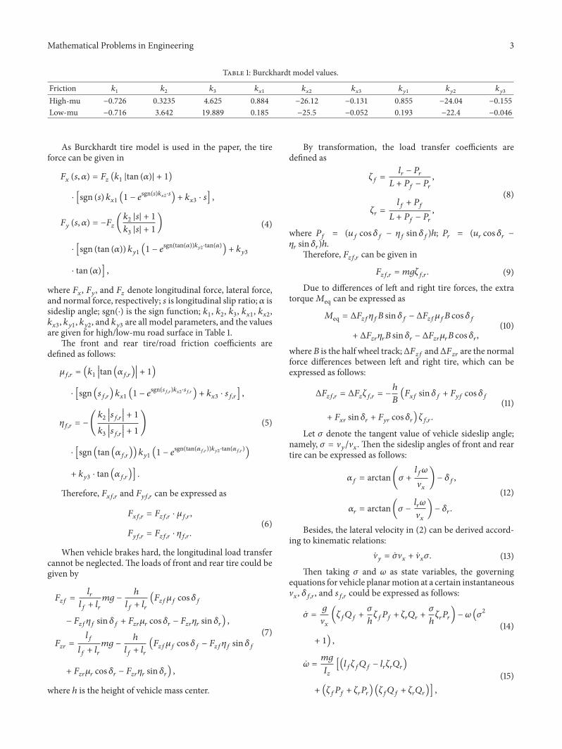
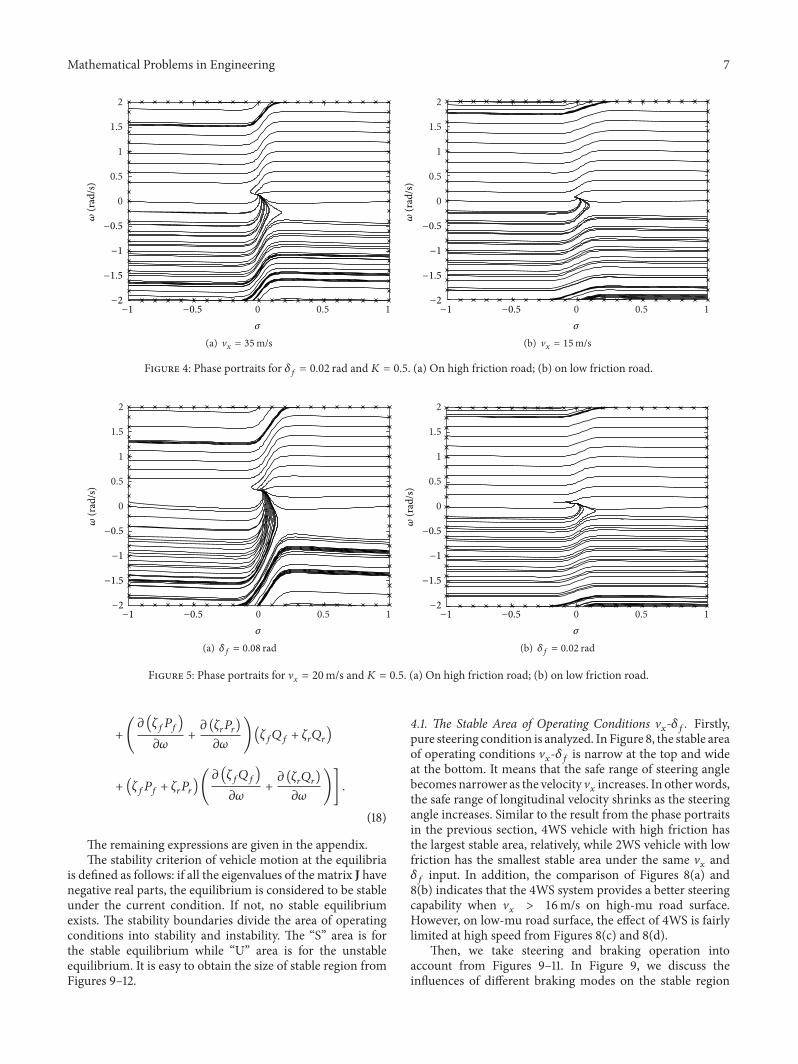
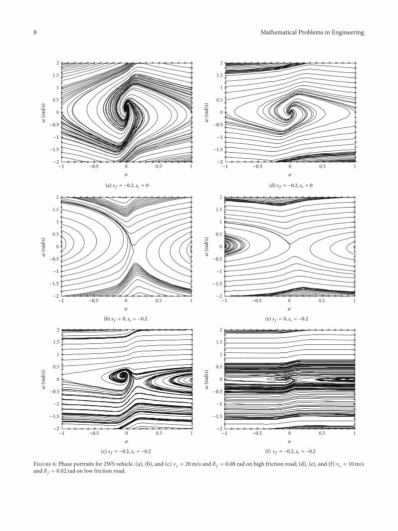
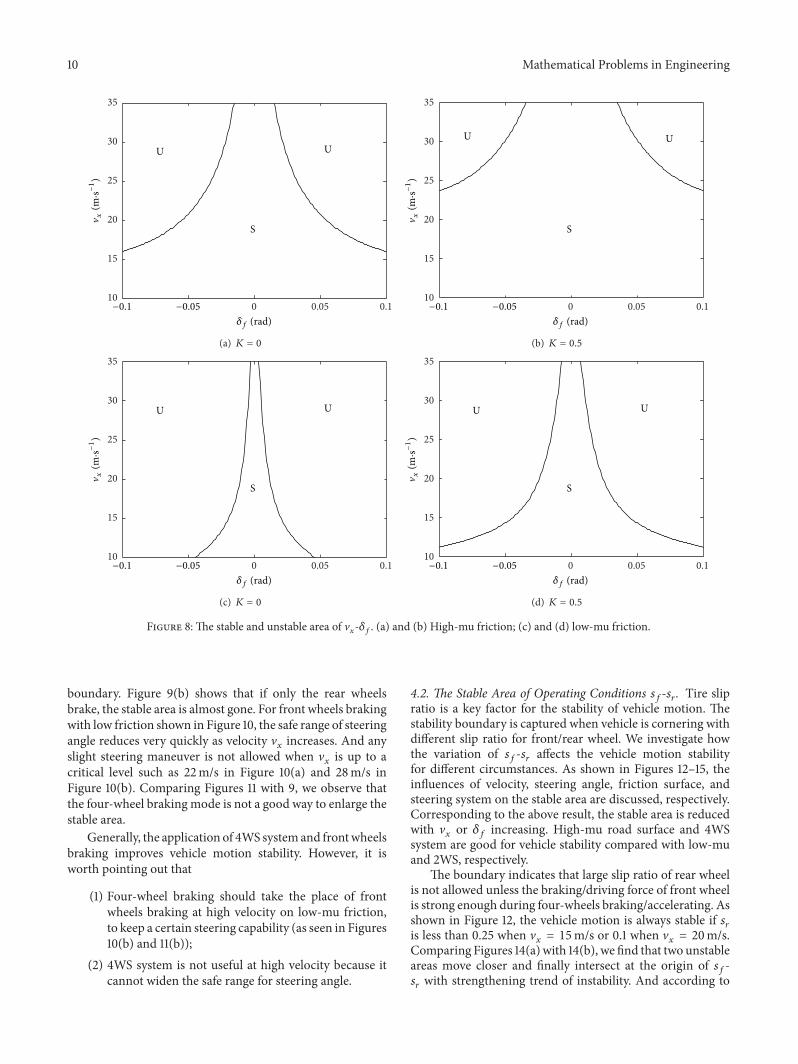
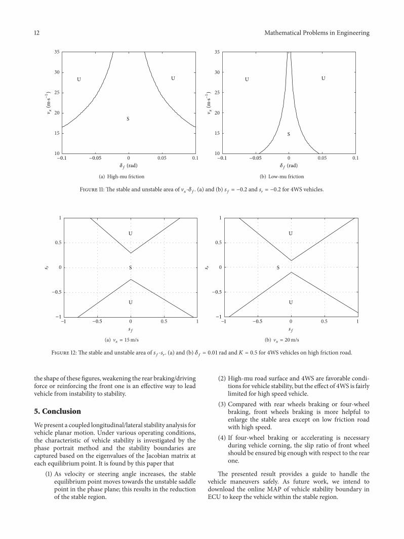
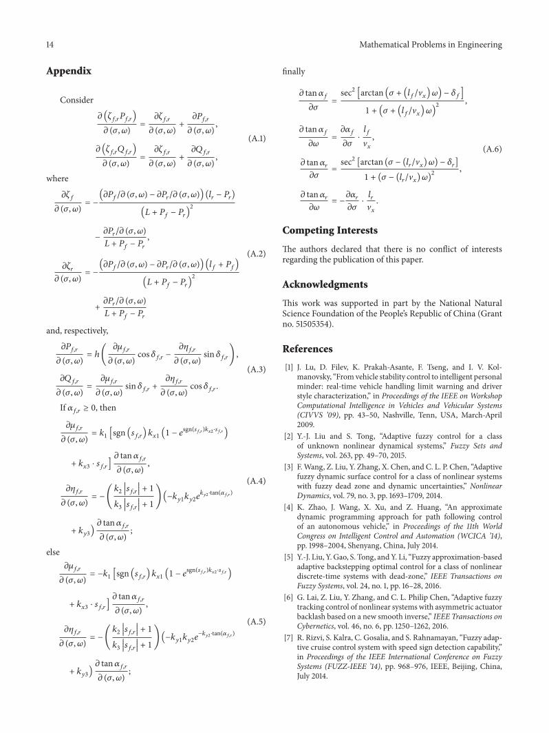