Performance Prediction of a Turbo-coded Link in …lib.tkk.fi/Dipl/2010/urn100233.pdfPerformance...

AALTO UNIVERSITY SCHOOL OF SCIENCE AND TECHNOLOGYDepartment of Communications and Networking

Muhammad Moiz Anis

Performance Prediction of a Turbo-coded Link

in Fading Channels

Master’s Thesis submitted in partial fulfillment of the requirements for the degreeof Master of Science in Technology.

Otaniemi, Espoo. March 23rd, 2010

Supervisor: Professor Olav Tirkkonen

Instructor: Helka-Liina Maattanen, M.Sc. (Tech.)

AALTO UNIVERSITY SCHOOL ABSTRACT OF THEOF SCIENCE AND TECHNOLOGY MASTER’S THESIS

Author: Muhammad Moiz Anis

Name of the Thesis: Performance Prediction of a Turbo-coded Link

in Fading Channels

Date: March 23rd, 2010 Number of pages: 78

Department: Department of Communications and Networking

Professorship: S-72

Supervisor: Prof. Olav Tirkkonen

Instructor: Helka-Liina Maattanen, M.Sc. (Tech.)

Channel coding is the method of adding redundancy to the data in order to reducethe frequency of errors or to increase the capacity of a channel. Turbo codes are themost superior class of codes making achievable channel capacity almost at par with theShannon limits. In Adaptive Modulation and Coding (AMC) the prediction of errorperformance of a channel is an important step before choosing one of the ModulationCoding Scheme (MCS). Since in Turbo-coded system we donot have analytical relationsto relate error performance with the Signal to Noise Ratio (SNR). Therefore, normallysimulation results are stored in the form of the look up tables.

In this work we propose an error performance prediction model for a BPSK modu-lated Turbo-coded link. This model predicts performance addressing the fading phe-nomena for wireless radio channels. It takes the large variations in the SNR level withina code block into account along with the coding parameters. The SNR dB values pro-file inside a code block is considered in terms of their mean and variance. The modelproposed is UMTS compliant and is continuous for values of the MCS code rate and themean and variance of SNR dB values. It is an easier way of predicting link level per-formance as it replaces the discrete look up tables. Unlike the look-up tables it can beused for differentiation based analytical techniques used in system level optimization.

Keywords: Fading, BLER, effective SNR, mean, variance, Turbo-codes.

ii

I would like to dedicate this work to the most perfect human being God ever created(according to my belief), the Prophet Muhammad (May peace be upon him)

iii

Acknowledgments

The driving force behind me, from the ideal evolution till the accomplishment of therealized targets in this work is my thesis supervisor Professor Olav Tirkkonen. Hissupport and confidence was an asset for me. In fact there were numerous occassionswhere his presence as a devoted mentor helped me greatly in maintaining my focus.His personality has always been a source of inspiration. I put forward my mostheartfelt gratitudes to him for being an examplery researcher. As a supervisor hewas so kind to accomodate me despite his busy schedule, for any sort of consultationregarding this work. I offer my earnest thanks to him for being a staunch supporterof every aspect of this work.

My thesis instructor MSc. Helka-Liina Maattanen also deserves my sincere thanksfor being very cooperative, supportive and friendly. I am in particular thankful forthe frequent reviews she did of this draft. Inspite of having her work seat in NokiaResearch Center (NRC), I feel indebted for her firmness in commitment and devotionto this work. In particular her advice regarding research work writing has provento be highly valuable. I am grateful to her for support and guidance in every phaseof this work.

Apart from these two personalities there are two other people who were also kindenough to help technically at various stages of this work. They are Mr. Kalle Ruttikand Mr. Sergio Lembo. Being my seniors, both were helpful in providing their valu-able advice and support. Particularly, Sergio deserves a special thanks for providinghis assistance in issues regarding the simulations involved in this work. I wouldlike to thank my roommates in the office: Anzil Abdul Rasheed, Iiro Jantunen andAlexander Renaud Pitawal for their pleasant and favourable presence throughoutthis work. It was always nice to listen about the Nordic and Finnish history fromIiro and chatting with Anzil during leisure time. Anzil was decent enough to give

iv

his advice in particular about thesis writing in Latex.

I am indebted to Mr. William Martin also for undertaking a thorough and valuablelanguage check up of this draft.

I regard my friends Umar, Maliha, Khurram, Zohaib and Farhan also for keepingme cheered up with their invigorating and joyful company.

I feel indebted to my parents for providing me with the best education, despitetheir limited resources, and carving a dignified character out of myself. Here, Icannot skip a whole-hearted thanks to the Finnish Government’s policy of freeeducation for foriegn students. It is laudable on part of the Finnish researchers’community also who welcomes foriegn researchers and students with open arms andgives them a chance to integrate and excel.

Otaniemi, Espoo. March 23rd, 2010

Muhammad Moiz Anis

v

Contents

Abbreviations ix

List of symbols xi

List of Figures xvii

List of Tables xviii

1 Introduction 1

1.1 Background . . . . . . . . . . . . . . . . . . . . . . . . . . . . . . . . 1

1.2 Contribution . . . . . . . . . . . . . . . . . . . . . . . . . . . . . . . 4

1.3 Structure and Organization . . . . . . . . . . . . . . . . . . . . . . . 5

2 Turbo coding 8

2.1 Introduction . . . . . . . . . . . . . . . . . . . . . . . . . . . . . . . . 8

2.1.1 Birth of Turbo codes . . . . . . . . . . . . . . . . . . . . . . . 8

2.2 Block Codes . . . . . . . . . . . . . . . . . . . . . . . . . . . . . . . . 9

2.3 Convolutional codes . . . . . . . . . . . . . . . . . . . . . . . . . . . 11

2.3.1 Convolutional Encoder . . . . . . . . . . . . . . . . . . . . . . 11

2.3.2 Viterbi Decoding algorithm . . . . . . . . . . . . . . . . . . . 14

2.4 Turbo Codes . . . . . . . . . . . . . . . . . . . . . . . . . . . . . . . 15

2.4.1 Turbo Encoder . . . . . . . . . . . . . . . . . . . . . . . . . . 17

2.4.2 Turbo Decoding . . . . . . . . . . . . . . . . . . . . . . . . . 18

2.4.3 Maximum A-Posteriori (MAP) Decoding Algorithm . . . . . 21

2.4.4 MAP Derivatives: Log MAP and Max Log MAP . . . . . . . 23

2.4.5 Soft Output Viterbi Algorithm (SOVA) for decoding . . . . . 25

2.5 Conclusion . . . . . . . . . . . . . . . . . . . . . . . . . . . . . . . . 25

vi

3 Error Performance of Turbo-coded BPSK Link 26

3.1 Shannon´s Error Free Channel . . . . . . . . . . . . . . . . . . . . . 26

3.2 Error Performance of Memory-less Modulation Signals . . . . . . . . 27

3.2.1 Binary Modulation Systems . . . . . . . . . . . . . . . . . . . 27

3.2.2 BPSK Modulation System in Fading Channel . . . . . . . . . 30

3.3 Turbo Coded BPSK . . . . . . . . . . . . . . . . . . . . . . . . . . . 30

3.3.1 AWGN or Non-Fading Channel . . . . . . . . . . . . . . . . . 31

3.3.2 Fading Channel . . . . . . . . . . . . . . . . . . . . . . . . . . 35

3.4 Conclusion . . . . . . . . . . . . . . . . . . . . . . . . . . . . . . . . 36

4 Performance Prediction and Fading 38

4.1 Adaptive Modulation and Coding . . . . . . . . . . . . . . . . . . . . 39

4.2 Performance Prediction . . . . . . . . . . . . . . . . . . . . . . . . . 40

4.3 Fading channel . . . . . . . . . . . . . . . . . . . . . . . . . . . . . . 42

4.4 Varying SNR and Fading . . . . . . . . . . . . . . . . . . . . . . . . 42

4.4.1 Effective SNR Mapping . . . . . . . . . . . . . . . . . . . . . 43

4.4.2 Performance prediction Model for Fading Channels . . . . . . 44

4.5 Conclusion . . . . . . . . . . . . . . . . . . . . . . . . . . . . . . . . 46

5 Link Simulations 47

5.1 Link Layout . . . . . . . . . . . . . . . . . . . . . . . . . . . . . . . . 47

5.2 Two-peak Distribution . . . . . . . . . . . . . . . . . . . . . . . . . . 49

5.2.1 Mean and Variance Expressions . . . . . . . . . . . . . . . . . 50

5.2.2 Channel Coefficients . . . . . . . . . . . . . . . . . . . . . . . 51

5.3 Simulator Structure . . . . . . . . . . . . . . . . . . . . . . . . . . . 51

5.4 Simulation Issues . . . . . . . . . . . . . . . . . . . . . . . . . . . . . 53

5.4.1 1000 snapshots approach and smoothness in performance curves 54

5.4.2 Linear average dB represented SNR on x-axis . . . . . . . . . 55

5.4.3 Curves for UMTS standard Turbo code in fading channels . . 55

5.4.4 Results Analysis . . . . . . . . . . . . . . . . . . . . . . . . . 55

5.5 SNR statistics vs Effective SNR value . . . . . . . . . . . . . . . . . 58

5.6 Conclusion . . . . . . . . . . . . . . . . . . . . . . . . . . . . . . . . 58

6 Curve Fitting 60

vii

6.1 Heuristic selection of a Sigmoid function . . . . . . . . . . . . . . . . 60

6.2 Modifications in Sigmoid function . . . . . . . . . . . . . . . . . . . . 61

6.2.1 G-factor . . . . . . . . . . . . . . . . . . . . . . . . . . . . . . 62

6.2.2 Flooring Effect . . . . . . . . . . . . . . . . . . . . . . . . . . 63

6.3 Cross Relationship between Code Rate and SNR Variance . . . . . . 65

6.4 Proposed Function . . . . . . . . . . . . . . . . . . . . . . . . . . . . 65

6.5 About Fitting Method . . . . . . . . . . . . . . . . . . . . . . . . . . 66

6.5.1 Fitting Metric . . . . . . . . . . . . . . . . . . . . . . . . . . 66

6.6 Optimal Form of the Function . . . . . . . . . . . . . . . . . . . . . . 67

6.7 Conclusion . . . . . . . . . . . . . . . . . . . . . . . . . . . . . . . . 68

6.8 Prospective Development . . . . . . . . . . . . . . . . . . . . . . . . 72

A Parametric Expressions for Four Statistical Numbers 73

Bibliography 76

viii

Abbreviations

AMC Adaptive Modulation and Coding

ARQ Automatic Repeat Request

AWGN Additive White Gaussian Noise

BCH Bose Chaudhuri Hocquenghem

BEC Backward Error Correction

BER Bit Error Rate

BLER Block Error Rate

BPSK Binary Phase Shift Keying

CODEC Coder and Decoder

CQI Channel Quality Indicator

CRC Cyclic Redundancy Codes

CSI Channel Side Information

ESM Effective SNR Mapping

FEC Forward Error Correction

LLR Log Likelihood Ratio

LTE Long Term Evolution

MAP Maximum A-Posteriori

MCS Modulation Coding Scheme

ix

MIMO Multiple Input Multiple Output

OFDMA Orthogonal Frequency Division Multiple Access

PC Power Control

PDF Probability Density Function

RMSE Root Mean Square Error

RS Reed Solomon

SOVA Soft Output Viterbi Algorithm

SSE Sum of Square Error

UMTS Universal Mobile Telecommunication System

WiMAX Worldwide Interoperability for Microwave Access

3G Third Generation

4G Fourth Generation

3GPP 3rd Generation Partnership Project

x

List of symbols

m Mean of dB SNR distribution inside Codeblock

v Variance of dB SNR distribution insideCode block

m1 Mean of the first constituent distributionof the two peak distribution

v1 Variance of the first constituent distribu-tion of the two peak distribution

m2 Mean of the second constituent distribu-tion of the two peak distribution

v2 Variance of the second constituent distri-bution of the two peak distribution

p A fractional number used to control theweightage between the two constituentdistributions of the two peak distribution

n Total number of bits per code block

k Number of information bits per code block

np Number of parity bits generated by eachconstituent encoder

R Code rate

K Number of shift registers

xi

CL Number of bits in encoder memory or con-straint length

g Generator polynomial coefficients vector

g(z) Generator polynomial

z1 Representing first memory stage or shiftregister in generator polynomial

z2 Representing second memory stage orshift register in generator polynomial

bi Input bit

bp Parity bit

s1 State of first shift register

s2 State of second shift register

J Stage of time or clock

xk Set of input information bits for a turboencoder

x′k Set of interleaved version of the input in-

formation bits for a turbo encoder

zk Set of parity bits generated by first RSCencoder

z′k Set of parity bits generated by second

RSC encoder

uk Representing an encoded symbol whichmay be +1 or -1 for a 1 or 0 informationor parity bit

L(uk) LLR corresponding to each uk

y′

Received symbol sequence

Sk−1 Previous state of the registers

xii

Sk Current state of the registers

s The final state of a considered transition

s′

The initial state of a considered transition

αk−1(s′) The probability of being in state s

′at time

k − 1

βk(s) The probability of being in state s at timek

ϕk(s′, s) The probability of transition from s

′to s

γ Signal to Noise Ratio, SNR

xi Set of probability numbers to be appliedwith Max-Log-MAP approximation

fc Correction factor introduced in Max-Log-MAP approximation for Log-MAP

ν Corrected approximation function by Log-MAP

Eb, εb Transmitted (or coded) bit energy

Ebi Information bit energy

N0 Twice of gaussian noise spectral density

r Received signal

s0 Signal level associated with a ’0’

s1 Signal level associated with a ’1’

p(r/s0) Probability of signal reception given signaltransmitted is s0

p(r/s1) Probability of signal reception given signaltransmitted is s1

d12 Intersymbol distance

Pb Error probability

xiii

rl(t) Received signal in one signaling interval

sl(t) Transmitted signal in one signaling inter-val

η(t) Received signal in one signaling interval

µ Amplitude of fading coefficients, consider-ing them as complex numbers

φ Angle of fading coefficients, consideringthem as complex numbers

γb SNR per bit

p(γb) Probability density function of SNR perbit

P2(γb) Bit error for BPSK modulated signalswhen µ is fixed

Pe Bit error for BPSK modulated signalswhen µ is variable

γmean Mean SNR value

L Bad estimate of reliability factor

Lc Correct reliability factor

X Linear factor i.e. ratio of L to Lc

L(yk|xk) Conditional log likelihood ratio or Softoutput through the channel

a and ak Fading channel amplitude response coeffi-cient vector

M Magnitude of signal

BW Signal bandwidth

yk Channel ouput vector following matchedfilter approximation

xiv

σ2 Noise variance

B Block length

γeff Effective value of SNR, when channeldoesnot have a uniform state inside codeblock

fSNR(γ) Probability Density Function (PDF) forcontinuous channel symbol SNR values

pi Probability mass function for discreteSNR values

I(γ) Information measure

N Number of times loop running for theMonte carlo simulation

S Skewness of dB SNR distribution insidecode block

K Kurtosis of dB SNR distribution insidecode block

c1-c4, k1-k21 Parameters used in curve fitting

a′, a1, a2, b

′, b1, b2 and G Constant numbers used for illustrative ex-

planation of different curve fitting mecha-nisms

xv

List of Figures

2.1 Block code composition . . . . . . . . . . . . . . . . . . . . . . . . . 11

2.2 a 0.5 rate Convolutional Encoder with state transition diagram, [14] 13

2.3 Trellis diagram for the Encoder shown in Figure 2.2 . . . . . . . . . 14

2.4 Trellis Viterbi decoding for the encoder shown in Figure 2.2 . . . . . 16

2.5 Turbo encoder comprising of 2 identical RSC encoders [3] . . . . . . 17

2.6 Effect of the number of iterations on BER curve [14] . . . . . . . . . 18

2.7 A typical turbo decoder . . . . . . . . . . . . . . . . . . . . . . . . . 19

2.8 Possible transitions for K=3 RSC encoder [14] . . . . . . . . . . . . . 22

2.9 Possible transitions for K=3 RSC encoder [14] . . . . . . . . . . . . . 23

3.1 PDFs of two binary symbols [25] . . . . . . . . . . . . . . . . . . . . 28

3.2 Error probability comparison for binary signals . . . . . . . . . . . . 29

3.3 Error probability comparison between AWGN and Rayleigh fadingchannel . . . . . . . . . . . . . . . . . . . . . . . . . . . . . . . . . . 31

3.4 BER performance for different decoding algorithms [14] . . . . . . . 32

3.5 Performance at different code rates realized by different numbers ofpunctured parity bits, [14] . . . . . . . . . . . . . . . . . . . . . . . 33

3.6 Effect of framelength on BER performance [14] . . . . . . . . . . . . 33

3.7 Effect of channel reliability factor estimation [14] . . . . . . . . . . . 34

3.8 Performance at different code rates realized by different numbers ofpunctured parity bits [14] . . . . . . . . . . . . . . . . . . . . . . . . 36

3.9 Performance at different degrees of selectivity realized [12] . . . . . . 37

xvi

4.1 Example AMC scheme for a WiMAX base station . . . . . . . . . . 40

4.2 Example MCS set . . . . . . . . . . . . . . . . . . . . . . . . . . . . 41

4.3 Non-uniform SNR within a code block . . . . . . . . . . . . . . . . . 43

4.4 A comparison among different information measures [27] . . . . . . . 44

4.5 Error performance comparison for two different information mea-sures [27] . . . . . . . . . . . . . . . . . . . . . . . . . . . . . . . . . 45

5.1 Block diagram of the overall Link . . . . . . . . . . . . . . . . . . . . 48

5.2 PDF of a two-peak distribution: p=0.5,m1=-10,m2=5,v1=1,v2=3 . 49

5.3 Block diagram of the simulator . . . . . . . . . . . . . . . . . . . . . 52

5.4 Unreliable curves obtained in first attempt . . . . . . . . . . . . . . . 53

5.5 Smoother curves with scaling problem . . . . . . . . . . . . . . . . . 54

5.6 Plots with linear mean SNR in dB on x-axis . . . . . . . . . . . . . . 56

5.7 UMTS standard compliant curves for various code rates . . . . . . . 57

6.1 Oscillating polynomial fit over some data points . . . . . . . . . . . . 61

6.2 An example Sigmoid curve . . . . . . . . . . . . . . . . . . . . . . . . 61

6.3 A closer Sigmoid curve . . . . . . . . . . . . . . . . . . . . . . . . . . 62

6.4 Sigmoid curves of different slopes . . . . . . . . . . . . . . . . . . . . 62

6.5 Sigmoid curves for changing G in a semilog plot . . . . . . . . . . . . 63

6.6 Sigmoid curves for a known slope and position . . . . . . . . . . . . 64

6.7 Sigmoid curves with different levels of flooring effect . . . . . . . . . 64

6.8 Constant BLER surfaces . . . . . . . . . . . . . . . . . . . . . . . . . 65

6.9 Case 6: Fitting the simulated curves with 21 parameters . . . . . . . 71

xvii

List of Tables

6.1 Explanation of each Case . . . . . . . . . . . . . . . . . . . . . . . . 68

6.2 Parametric values and correpsonding Fitting metric for cases withoutG-factor . . . . . . . . . . . . . . . . . . . . . . . . . . . . . . . . . . 69

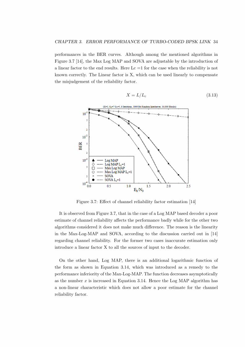
6.3 Parametric values and correpsonding Fitting metric for cases withG-factor . . . . . . . . . . . . . . . . . . . . . . . . . . . . . . . . . . 70

xviii

Chapter 1

Introduction

1.1 Background

In telecommunication applications wireless systems are preferred over wired onesdue to easy installation and maintenance, flexibility in reconfiguration, low costcomponents and mobility. In practice, however, a wireless channel is a less reliablemedia, in particular because of the fading in the radio channels. A signal in awireless channel becomes attenuated. Fading can be defined as the variation in thatattenuation which may vary with time, geographical location or radio frequency. Thevariations in the signal strength are classified as large and small scale variations in[28].

� Large scale variations, due to average path loss because of the distance trav-elled and shadowing by large objects such as buildings and hills. This is typi-cally frequency independent. It occurs when mobile moves through a distanceof the order of the cell size.

� Small scale variations, due to the constructive and destructive interferenceof the multiple versions of the same signal travelling through different pathsbetween the transmitter and receiver. This type of variation is frequencydependent.

The fading channels are normally classified as slow fading and fast fading channels.A channel is said to be fast fading if the coherence time of the channel is muchshorter than the delay requirements of the application, and is a slow fading channelif the coherence time is longer. Coherence time can be defined as the minimum timerequired to make the amplitude changes of signal uncorrelated with its previous

1

CHAPTER 1. INTRODUCTION 2

value [28].

Channel coding is the method of adding redundancy patterns to the signal for low-ering the error rate. If the data has too many errors for the desired use, then codingis used to attain a less frequent error rate or to attain a greater data rate. Wirelesssystems performance have gained enough improvement with channel coding. In par-ticular, with turbo codes achievable throughput is very close to the Shannon limitswhich was not possible before [15].

The now classic turbo-coding scheme is based on a composite Coder and Decoder,(CODEC) constituted by two parallel concatenated codecs. Since their invention,turbo codes have evolved at an unprecedented pace and have reached a state ofmaturity in a relatively short time scale. As a result, turbo coding has also beenstandardized in systems, such as, for example, the third-generation (3G) mobileradio systems.

To improve system performance, peak data rate and coverage reliability for aparticular link, the transmitted signal is modified to compensate for signal qualityvariations, a process which is called Link Adaptation. It means changing transmis-sion parameters over a link, such as modulation, coding rate, power, etc., in responseto changing channel conditions. It is a powerful means of achieving higher efficiencyor throughput in wireless networks.

Adaptive Modulation/Coding, (AMC), Adaptive Power Allocation and WaterFilling are some of the example of Link Adaptation techniques. According to theliterature review in [2], among these techniques AMC is considered attractive be-cause of its simplicity and high performance. The adaptation of the transmissionparameters is performed according to the predicted future performance. To rendersuch a performance prediction, there is the need for a realistic model which maygive a good prediction of the error rate for a known value of Signal to Noise Ratio,(SNR).

Unfortunately, in coded systems analytical relationships, which may define all theresulting performance curves for different combinations of the code parameters likecode rate and block length, for instance, are not derivable. Therefore, to study suchsystems exhaustive computer simulations are required. A comprehensive simulationis essential, but inclusion of modelling of precise phenomena for each of the link


been simulated poses huge computational demands. Therefore, there are link andsystem level type simulations.

Link level simulations undertake a detailed modelling of all the steps involved fromthe generation till the reception and comprehension of digitized information at thereceiver passing through the wireless medium. Example phenomena include signalgeneration, signal encoding, signal modulation, channel modelling, detection anddemodulation of the signal as well as signal decoding. The essentiality of segregatingsimulations is more for the case of turbo-coded systems where in particular the turbodecoding operation is the most resource consuming part of the simulators. Theresults obtained are often stored in the form of a look-up table or a mathematicalfunction, which are then used in system simulations.

System level simulations depict the overall view of a wireless system. In this kindof simulation, all the phenomena at the level of a single link are approximated onthe basis of the results coming from link level simulations. Authenticity of systemlevel simulations is dependent on the precision of results at link level. Also thetask of optimizing system parameters can be inefficient and difficult if the margin ofimplementing optimization algorithms over link level results is narrow. For instance,derivative-based optimization techniques can only be used if we have a continuousfunction, for reproducing link level simulation results.

In system level simulations all the link level details are normally hidden behindthe relationship defining a system level parameter called Block Error Rate, BLER,defined in terms of Signal to Noise Ratio, which is a link parameter. The first andeasier choice for efficient utilization of simulation results would be to maintain look-up tables. But using these will restrict system level simulations for discrete or evena limited set of code rates.

A better idea is of forming a mathematical model for performance evaluation.This method of modelling the coded systems’ performance can be found in [19]and [20]. In the mentioned work the channel is considered to be as Additive WhiteGaussian Noise, (AWGN) channel. In an AWGN channel, where it has a constantadditive white noise and amplitude response is 1, SNR mapping is not challengingand the channel within a block does not vary. Therefore, in the mentioned work theperformance of coded systems is considered against coding parameters. For instance,the considered coding parameters are code rate, block length and puncturing pattern


in [20].

The case with fading is not that simple. In fading channels a block length mayexperience mutiple channel states. In other words, there may be multiple valuesof SNR for groups of bits or even bit specific values of SNR inside a code block.The presence of fading mainly deteriorates the performance, but along with thisdeterioration, SNR to error performance mapping is also vague. In [27] the ideaof having an effective SNR is considered. In this work an averaging term calledthe information measure is introduced which is then defined in five different forms.Finally, it proves a mutual information averaging measure to provide the best resultsfor turbo codes.

1.2 Contribution

The idea is to establish a relationship of the turbo coded system performance withthe statistics of the SNR distribution i.e. mean and variance. Here instead of goingfor a complicated evaluation of the effective SNR, the SNR distribution within ablock has been represented by two statistical numbers. In order to trace a relation-ship of the link performance with the mean and variance of the SNR dB values insidea code block and code rate, a ready made turbo coded link simulator for AWGNchannel with Binary Phase Shift Keying (BPSK) as the modulation scheme, wasmodified for fading channels.

In the pursuit of the targetsoutlined above, a straight route would have been torealize various conventional fading realizations and then calculate and record eachrealizations higher order statistics for simulations. But this strategy would have ledto a very exhaustive exercise. Instead, an SNR distribution has been assumed, whichis a weighted sum of two normal gaussian distributions. Hence, considering the meanand variance of each of the two distributions with the weightage parameter, thereare five parameters (i.e. the mean and variance of the first normal distribution, m1,v1, the mean and variance of the second normal distribution, m2, v2 and the scalingfactor p) which are needed to define this distribution.

In our investigation we are concerned about the mean and variance of the SNRdistribution generated using these five parameters. Therefore, formulae for meanand variance of the distribution were derived in terms of these parameters and twoequations were then solved to find each of the five parameters in terms of the mean


and variance of the distribution. This enables a SNR number series to be generatedfor a known set of the mean and variance of the SNR distribution. These SNRnumbers are generated in the dB domain.

As a final task of this work, we fit curves to the obtained simulation results inorder to acheive a mathematical relationship relating SNR to BLER along withtaking into account the code rate and variance of the SNR values profile inside thecode block. We take a nonlinear Sigmoidal curve with some suitable modificationsand fit it over the simulation results in a least square sense, for a modified fittingmetric. The modifictaion in the fitting metric is made to suit the semilog plotswhich are used to plot the SNR vs BLER relationship.

1.3 Structure and Organization

The structure of this thesis is arranged in a fashion to develop a gradual understand-ing of the topic by first starting with the pedagogical background and research workand then elevating it to a decent demonstration of the model, developed through thecourse of this work. Therefore, Chapter 2 is devoted to the introduction of turbocodes. In this chapter we explain the historical causes of the birth of turbo codes.In order to appreciate the superiority of turbo codes, it is important to have a goodidea of the codes in use in the era prior to turbo codes. Therefore, suitable attentionis given to both block codes and convolutional codes as well. In this chapter twoof the most well known decoding algorithms: Viterbi and Maximum A Posteriori,(MAP) have also been explained.

In Chapter 3, the performance of turbo codes in both fading and non fadingchannels is the topic. First, performance of uncoded modulation signals is explained.The inclusion of the discussion about uncoded systems has just been made to makethe reader appreciate the ample contrast between the performance of a coded andan uncoded systems and to realize the fact that the behaviours of coded systemsare studied via simulation plots because of the lack of analytical relations whichwould have explained performance. The presence of fading causing depreciation inthe performance of a radio link is another important issue discussed in this chapter.

In Chapter 4, the concept of performance prediction and its importance in theapplication of link adaptation techniques has been discussed. Apart from the con-cept of performance prediction, the problem of having multiple SNR values inside


a code block has been discussed. Here the established technique of effective SNRMapping has also been explained along with the presentation of the main idea ofthis work. A comparative analysis of the two techniques is also undertaken in thischapter.

In Chapter 5, the channel model used to characterize fading in terms of theSNR dB mean and SNR dB variance in a turbo coded link simulator has beenconceptualized, followed by a prior discussion about the overall link layout andfading affecting the SNR level inside a code block. The concept of the channel modelis supported with mathematical relations for terms like Log Likelihood Ratios andchannel coefficients. The chapter also contains the practical issues and other findingsevolved during the simulations. In Figure 5.7 the final results are demonstratedcomprising of several performance curves on a semilog plot between Block ErrorRate (BLER) and mean SNR dB, where each curve is associated with a particularcode rate and SNR dB variance.

Chapter 6, deals with the curve fitting of a heuristically selected mathematicalfunction over the obtained simulation curves. First, the reason for selecting thementioned function is discussed, then the initial modification introduced to theSigmoid is explained. The G-factor has been described as the way of changingthe slope and position of a Sigmoid. Also the neccessity of having an additionalexponential in the denominator has been emphasized to ensure that the Sigmoidalso caters for the flooring effect present in the simulation results. In the final stepa thorough optimization of all 12 possible combinations have been performed toobtain the best fit.

Conclusively, the model obtained as a result of the curve fitting over the simulationresults is mouldable by changing the number of the parameters used. Any of thefirst six cases out of the total twelve, can be used as working model. The choiceof the case shall be a trade off between the required accuracy and the maximumaffordable numbers of parameters. The reason of not using last six cases is becauseof the presence of an additional parameter i.e. G-factor which deteriorates fittinginstead of improving it.

As a prospective work it is possible to undertake an investigation or modelling withhigher statistical numbers of the SNR numbers inside a code block. It is essential, ifa fair comparison can be done with a common channel for the developed model with


effective SNR based predictor. Such comparison may also help in determining theexact number of statistical numbers for SNR values representation (inside a codeblock) required to define the performance in selective or fading channels.

Chapter 2

Turbo coding

2.1 Introduction

Information bits transmitted through a communication channel are corrupted bychannel variations and noise. If there are too many errors the intended messageis misunderstood or not undertood at all. There can be two ways to take countermeasures. Either the error is recognized only and the erroneous part is lost or errorsare corrected through proper Error Correction techniques. There are two strategiesfollowed for error correction, i.e. Forward Error Correction (FEC) and BackwardError Correction (BEC). Forward error correction can be defined as the error cor-rection method in which each dataword is supposed to have some bits dedicatedfor detecting and correcting errors in the original message. Parallel to that there isanother error correction method called the backward error correction method. Inthis method in the event of any error, the receiver makes a retransmission request tothe transmitter.This error control strategy is also called Automatic Repeat Request(ARQ). [6]

2.1.1 Birth of Turbo codes

In 1948 Shannon laid the foundations of error correction coding. He stated thepossibility of a nearly error free transmission over realistic channels by adding someauxiliary information. Historically, the birth of turbo codes is followed by the in-vention of block codes and convolutional codes, both of which shall be explained indetail in Sections 2.2 and 2.3 respectively. The block codes and convolutional codeshave passed through different stages of development in the same period of time.For instance, in 1950 Hamming code was the first single error correcting block codedevised [13]. During 1955 Elias discovered Convolutional codes [14].

8

CHAPTER 2. TURBO CODING 9

In 1967 a maximum likelihood estimation algorithm was introduced by Viterbi fordecoding convolutional codes. The algorithm was later interpreted by Forney. In1970 the first practical application of the Viterbi algorithm with convolutional codeswas proposed by Heller and Jacobs. The Maximum A-Posteriori (MAP) decodingalgorithm was proposed in 1974. This algorithm offers relatively lesser BER, theperformance margin between Viterbi algorithm decoding and MAP decoding beingvery narrow. MAP has been found to be far more complex for implementation,therefore MAP algorithm had been very rarely implemented till the evolution ofturbo codes [14].

Around 1960, the first multiple error correcting block code, Bose Chaudhuri Hoc-quenghem (BCH) was proposed [5], and then later in the same year eponymousReed Solomon (RS) codes were introduced. The RS codes are a non-binary subsetof BCH codes.

In 1968 Berlekamp appeared as the one proposing a range of decoding algorithmsfor the RS and BCH codes [26]. Also from the same era, evidence of soft decisiondecoding algorithms cannot be neglected. This was mainly proposed by Sweeneyand Honary. The RS codes had also been standardized for various applicationsincluding CD players and Digital Video Broadcasting.

The standardization of FEC for radio mobile systems dates back to the 1980s.During 1993 with the arrival of turbo codes, the operation of communication systemsclose to the Shannon limits became possible. Turbo codes were also adopted asthe standard for the ratified Third Generation (3G) mobile radio systems. Alsoadopted were the same binary turbo codes in the 3rd Generation Partnership Project(3GPP) Long Term Evolution (LTE) and duo-binary turbo codes in WorldwideInteroperability for Microwave Access (WiMAX) as mentioned in [18], [8] and [30].And for Fourth Generation (4G) standardization, the presence of turbo codes iscertain and is expected to undergo further evolutions.

2.2 Block Codes

Block codes are refered to as (n,k) codes, as it generates n-bits blocks for any k-bitsof information. Block codes are defined as one of the error correction codes havinga fixed length of encoded block generated by the encoder against a fixed length of


input data word. The ratio of the number of information bits k, to the total numberof bits n is defined as code rate R is

R =k

n=

k

k + np. (2.1)

The total number of bits of an encoded block is the sum of the information bitsk and the parity bits np, where parity bits are the additional or redundant bitsdecided according to the coding algorithm. For uncoded case n = k and so thereare no parity bits, i.e. np = 0.

In a code, a sequence of symbols assembled in accordance with the specfic rules ofthe code and assigned a unique meaning is called a code word. Linearity for a codecan be proven if the sum of the two code words results in a third valid code wordof the same coding scheme. Most of the block codes are defined to be linear, themost well-known example of linear block codes being Cyclic codes. This is becausethe hardware limitaions often make difficult the attainment of long code words. Inthis regard the cyclic codes are very important in providing a very practical way ofattaining long code lengths. Mathematically, a linear code is called cyclic only if acyclic shift on the code word results in another code word.

A well known class of Cyclic codes is Cyclic Redundancy Codes (CRC). CRC helpsin detecting all single bit errors, any odd number of errors and a burst of errors ifthe burst length does not exceed the number of check bits.

The two most common examples of block codes are Reed Solomon (RS) and Bose-Chaudhury-Hockquenghem (BCH) block codes. Both of them are mathematicallybased on finite field structures. The finite fields have a limited number of elements.The field is supposed to be closed under the operations been defined for it, i.e. theresult of any operation on any two elements of the field is also supposed to be anelement of the field.

Reed Solomon (RS) is a multiple error correcting code. It can be defined as anon-binary sub class of the BCH code. RS code is a cyclic code i.e. any cycle shiftedversion of a code word is also a code word. Similarly, a linear combination of somecode words also forms another code word.

A code having code words with parity bits which are easily distinguishable is calledSystematic code. For purposes of illustration, we take an example of a systematic


Figure 2.1: Block code composition

code word. Figure 2.1 shows the composition of a typical block code’s code word.Improvement in the number of correctable errors requires more parity bits to beadded, which is not expandable to a very high number due to computational powerconstraints.

2.3 Convolutional codes

The concept of convolutional coding is more than half a century old. Since the timeof inception it has been being considered as one of the few most efficient Forwarderror correction codes. The name convolutional code result from their resemblancein operation to a filtering or convolution operation. Unlike block codes, however,they can be applied for coding streams of data and the code rate is the same asdefined in Equation 2.1.

2.3.1 Convolutional Encoder

Unlike, the block codes where blocks of data are mapped into (longer) blocks ofdata, in convolutional codes the encoder maps (in principle continuous and infinite)streams of data into more streams of data. This mapping is realized by sending thedata streams over linear filters [22].

If the input data stream is unaltered with in the output streams, then the con-volutional encoder is said to be systematic. The term recursive or non-recursive as-sociated with the convolutional encoders comes from their resemblance to a typicalfilter layout. The most important convolutional encoders in the context of iterativealgorithm is the binary systematic recursive convolutional encoder [22], since theyare the constituent components of the standard turbo codes.

Although [14] discusses block code based turbo codes, at low code rate, however,turbo codes with block codes based constituent encoders have high decoding com-plexity. Particularly, for code rates less than 2/3, turbo codes having convolutionalcode based constituent encoders are preferred [11].


A convolutional encoder is defined by (n, k,K), where K is the number of shiftregisters, the number of bits in the encoder memory or constraint length, CL is de-termined by the number of shift register stages affecting the generation of n encodedoutput bits. L is given as

L = K + 1, (2.2)

To generate n bits we need n polynomial generators. The generator polynomialsare constituted by a bit pattern determining the presence, or absence, of a link fromeach buffering stage. There are three memory or buffering stages in the encodershown in Figure 2.2, i.e. the buffered input and the two outputs of the two shiftregisters. As a new bit enters the input, all the three bits in series are right shifted.As an example the generator polynomial for the encoder in Figure 2.2 can be givenas g = [111], this is because the only modulo-2 addition block takes input from allthree memory stages. The polynomial can be given as,

g(z) = 1 + 1z1 + 1z2. (2.3)

We take the example of a half rate convolutional encoder with a number of in-formation bits, k = 1, R = 1/2 with a memory of three binary stages which makesthe number of shift registers to be two, i.e. K = 2 and the convolutional code canbe represented as (2, 1, 2). In Figure 2.2(a) this encoder is shown for the first tenclock cycles. The boxes marked s1 and s2 are the shift registers and the addition isa modulo-2 sum operator. Once a bit stages a register, the output then depends ona predetermined manner of the structure of the encoder and the output bit sequeceis thus not arbitrary. The number of valid output bit patterns is limited which helpsin the decoding process [14].

In Figure 2.2(b) the state transition diagram is presented which demonstratesthe possible transitions for each state as function of the incoming information bit,i.e. bi. In Figure 2.2(a) the corresponding parity bit, bp generated against can alsobe observed for the first ten clock pulses. The considered input bit stream is alsomentioned. In Figure 2.2(b) the broken lines represent bi = 1 and for solid linebi = 0.

From the inherent constraint, i.e. two shift registers, there are only two possiblestates where a transition can be made to. Another simpler way to represent theencoder is a trellis diagram. Figure 2.3 shows the trellis for the encoder in Figure 2.2.In Figure 2.3 the bit stream shown in Figure 2.2(a) is considered, the transition


(a) 0.5 rate turbo encoder

(b) State Transition Diagram

Figure 2.2: a 0.5 rate Convolutional Encoder with state transition diagram, [14]

against bi = 1 is represented with a broken line and vice versa. Moreover, thetransitions represented against each Jth stage of time or clock, in the diagram,strictly follows the transition constraints depicted in Figure 2.2(b).


Figure 2.3: Trellis diagram for the Encoder shown in Figure 2.2

2.3.2 Viterbi Decoding algorithm

The Viterbi decoding algorithm was proposed in 1967 and it basically performsmaximum likelihood decoding, although the computational load is reduced becauseof the special structure of the code trellis. In order to understand the Viterbidecoding method we need to consider the code trellis shown in Figure 2.4. Forsimplification, we consider all the zeros bit stream to be transmitted and the receivedbits have been detected and sent to the decoder. Hamming distance between thetwo binary numbers is measured in terms of the count of different correspondingbits. In the context of Viterbi decoding this hamming distance is the branch metric.

In the Figure 2.4 the two bit number associated to each branch is the encodedouput number i.e. bi, bp. As in the diagram all possible paths can be found nowwhen the received number enters the decoder in the form of a two bit symbol.It evaluates the cumulative branch metric at every dot if lying on a path. Forexample, in the Figure 2.4 it received 01 which has a hamming distance of 1 withboth possible output numbers 00 and 11 corresponding to the two possible transitionstates according to Figure 2.2(b), i.e. 00 for bi = 0 and 10 for bi = 1. Note that weassumed the initial state of both of the shift registers to be 00. At this stage, thedecoder is unable to express any preference as both paths have the same hammingdistance.


Proceeding to the second two bit symbol we assume to receive 00 and for thisnumber we have now four candidate branch metrics and they are found to 0,2,1 and1. The correponding cumulative branch metrics on the four paths at J = 3 are 1,3,2and 2. At this stage the upper most path can be singled out as the most likely pathbecause of the least distance of the encoded bits to the received bits. This is due tothe fact that there exist some finite probability for the other three paths.

The third symbol is assumed to be 10 and, accordingly, the cumulative branchmetrics are evaluated at this stage. It can be noticed their exist many mergingpaths giving multiple cumulative branching metric values to the same nodes. Inthis situation the less likely path or more distant path is dropped, for example atthe top node when J = 4 we see a merger of 00, 00, and 00 with the 11, 01 and01 path. Here the former is kept because of the lesser branch metric and such apath is called a survivor path. Similarly, if two paths merge at a node and givethe same metric, then a random selection can be made. In the considered examplealthough it does not affect if any of the path in the bottom at J = 4 in Figure 2.4is taken. Because the top most path, indicated with a darker line, is already withleast cumulative metric value and is supposedly the winning path.

In some cases, however, it might lead to errors to have random selections. Thedecision taken on the basis of the complete information sequence is best, although anearly decision help reducing latency. Practically it has been found that the bit errorrate is virtually unaffected by curtailing the decision interval to about five timesthe encoder ’s memory [14] which is three in the discussed example. The associatedbranch metric for the winning path is also the number of the transmission error.The winning path is the one shown with a darker line in Figure 2.4.

2.4 Turbo Codes

The term Turbo was selected by the inventors in order to emphasize the operation ofthe codes as reminiscent of the turbo charging of an automobile via engine-heated orexhausted air been fed back to the air intake resulting an increased efficiency. Thereis a trade off between complexity and performance. By increasing the codelength,the ability of the code to detect and correct error improves but at the same timedecoding complexity increases. Also the hardware design faces fierce challenges andconstraints due to the limited processing power, specifically for a general purposeprocessor. Fortunately, turbo codes maintain a very reasonable decoding complexity


Figure 2.4: Trellis Viterbi decoding for the encoder shown in Figure 2.2


Figure 2.5: Turbo encoder comprising of 2 identical RSC encoders [3]

for a very long code length, which has made possible the code performance beingalmost on par with the Shannon limits, which were hypothetical just before turbocodes were introduced in 1993.

2.4.1 Turbo Encoder

A standard turbo encoder can be thought of comprising a minimum of two convo-lutional encoders, the most popular choice is Recursive Systematic Convolutional,RSC, encoders. The two RSCs have an inter-leaver between them which makesthem statistically independent of each other. Each RSC generates encoded wordscomprising of some parity bits along with the information bits. These parity bitscan then variably be punctured to realize various code rates. As an example, ifthe two RSCs were half rate, then puncturing half of the parity bits of each RSCmakes the overall coderate to be half. Similarly, if both parity bit sets were takenunpunctured then the overall coderate would be one-third.

In Figure 2.5 there are two identical RSC encoders, each of them generating a setof parity bits, xk is the set of input information bits with zk which is a set of paritybits generated for xk by the first constituent RSC encoder. Similarly, x

′k shown in

dotted lines is the interleaved version of the input information bits and z′k is the set

of parity bits generated by the second RSC encoder.


Figure 2.6: Effect of the number of iterations on BER curve [14]

2.4.2 Turbo Decoding

One of the most favourable points in the development of turbo codes was the incep-tion of the iterative decoding algorithm. In this algorithm, the decoders iterativelyoperate on the received data. The greater the number of iterations, the more ac-curate are the results. Here the a-priori symbol probabilities from the encoder aremade available to the first decoder then the rest of the others receive the sameprobability and send it back to the first, also in a cycle, until some known and pre-decided number of iterations are completed and finally decide the transmitted codeword. The number of iterations increment improves system performance for a verysmall SNR but there is a limit to that gain. It has been observed that normallyafter 18 iterations further increase does not reflect significantly on the BER curve.Figure 2.6 depicts BER curves for a different number of iterations.

A typical decoder, as shown in Figure 2.7, comprises of two component decoderseach decoder taking three inputs. The first input is the systematically encodedchannel output bits, the second is the parity bits transmitted from the associatedcomponent encoder and the third is the information from the other componentdecoder about the likely values of the bits concerned.

These likely values are also known as the a-priori information from the fellowdecoder. This a-priori input comes through an inter-leaver if it is supposed to go to


Figure 2.7: A typical turbo decoder

a decoder which receives interleaved Systematic input. Similarly, a de-interleavedversion of the a-priori information is to be fed to the decoder which takes uninter-leaved systematic input. Each decoder is supposed to provide soft outputs alongwith the decoded bits.

During the first decoding attempt, the encoded input is decoded as a soft outputand then this soft output is fed to the second decoder which uses this soft outputalong with the encoded input to give a soft output to be fed to the first decoderwhich, this time, decodes the encoded input along with soft output from the secondcycle. This way it completes the first iteration. There are two popular turbo de-coding algorithms, the Maximum A-Posteriori (MAP) and the Soft Output ViterbiAlgorithm (SOVA).

Log Likelihood Ratios, (LLR) and Reliability Factor

The Log Likelihood Ratio of a data bit can be denoted as L(uk) where uk mayassume either +1 or -1. It is merely defined as the ratio of the probabilities of thebit taking its two possible values elaborated mathematically as,

L(uk) = ln

(P (uk = +1)P (uk = −1)

). (2.4)

Prior to decoding, the LLRs have to pass through some channel, where it is essen-tial to understand the importance of the reliabilty factor. For a BPSK modulation


case over some channel with the magnitude response coefficient(s) a, in [14] on page113, the LLR is given as,

L(yk/uk) =Eb2σ2

4ayk, (2.5)

where L(yk/uk) is the conditional log likelihood ratio and is also referred as thesoft output of the channel. It can be thought of as a product of the matched filterapproximated output of the channel denoted by yk, multiplied by the reliabilityfactor denoted by Lc. The reliability factor for the channel is given as,

Lc = 4aEb2σ2

. (2.6)

A matched filter approximated channel output can be expressed as in Equa-tion 2.7. If uk is the encoded signal, ηk is the Gaussian Noise, a is the channel’smagnitude response coefficient, which is equal to ’1’ for as Additive White GaussianNoise (AWGN) channel,

yk = auk + ηk [21]. (2.7)

In [21]on page 239 for a matched filter approximation, a detailed derivation relatesEbN0

and SNR as,

SNR =2EbN0

. (2.8)

The EbN0

used in the simulations for plotting curves is the one taking the informa-tion bit energy into account. The one considered in Equation 2.6, is related to thecoded bit energy. Mathematically, the coded bit energy, Eb is the product of thethe information bit energy, Ebi and code rate R,

Eb = EbiR. (2.9)

Multiplying both sides of Equation 2.9 by twice of the noise spectral density, i.e.N0,

EbN0

=EbiR

N0. (2.10)

From Equations 2.8and 2.10, the EbN0

used in simulations can be related to theSNR as,


γ =2EbiRN0

. (2.11)

Also in [21]on page 234 noise variance is defined in terms of noise spectral densityas,

σ2 =N0

2. (2.12)

From Equations 2.6, 2.8 and 2.12 the reliability factor in terms of the SNR canbe given as,

Lc = 2aγ. (2.13)

Hence, it becomes evident now that channel reliability value only depends on theSNR and coefficients of the amplitude response of the channel.

2.4.3 Maximum A-Posteriori (MAP) Decoding Algorithm

According to [1] the fundamental edge that the Maximum a posteriori algorithm fordecoding has over the Viterbi is its ability to reduce symbol error rate contrary to thelater which makes only a minimal word error possible particularly for convolutionalcodes and does not neccessarily guarantee any plausible performance on the frontof symbol or bit error rate. Also in [29] Andrew J. Viterbi, further adds the MAPalgorithm to be the only one which attains an acceptable level of performance atEb/N0 within 1 dB of the value corresponding to the Shannon limits.

The MAP algorithm not only gives the estimated bit sequence but also the prob-ability of each bit that has been decoded correctly. This makes it naturally suitablefor turbo decode as explained in Section 2.4.2. The MAP algorithm gives a prob-ability for each decoded symbol or bit uk, whether it was -1 or +1 if the receivedsymbol sequence y

′is given. Mathematically, this is equivalent to finding the LLR

as shown in Equation 2.4. The mathematical depiction of the formerly explainedprobability can be given as,

L(uk|y′) = ln

(P (uk = +1|y′)P (uk = −1|y′)

), (2.14)

Consider Figure 2.8, where for a Recursive Systematic Convolutional (RSC) en-coder based turbo encoder comprising 3 Shift registers, all possible transitions areshown. The continuous lines represent the input bit to be -1 while the broken line


Figure 2.8: Possible transitions for K=3 RSC encoder [14]

is for a +1 value of the input bit. It can be observed that if the previous, Sk−1 andcurrent state, Sk, of the registers are known then the value of the input bit, uk canbe determined. Hence, the probability of the uk = +1 is going to be the sum ofall four cases in Figure 2.8 with broken lines. Therefore, Equation 2.14 after theapplication of the Bayes theorem can be given as,

L(uk|y′) = ln

∑(s′ ,s)=>uk=+1 P ((Sk−1 = s′)(Sk = s)y

′)∑

(s′ ,s)=>uk=−1 P ((Sk−1 = s′)(Sk = s)y′)

. (2.15)

Where (s′, s) => uk = +1 is the set transitions from the previous state to the

current state if uk = +1. Taking the individual probability of each transition oreach received symbol sequence, either any one from the numerator or denominatorof the Equation 2.15, can be divided into three sections: code word associated withpresent transition, y

′k, the received sequence prior to the present transition, y

′j<k and

the sequence following the present transition, y′j>k. The division can be visualized

in Figure 2.9.

Also the probability for each received sequence can be divided into three proba-bilities, represented as α, β and ϕ. Mathematically, these can be given as,

P ((Sk−1 = s′)(Sk = s)y

′) = P (s

′sy′) = βk(s)ϕk(s

′, s)αk−1(s

′). (2.16)

Where α is the probability for being in state s′

at time k− 1, y′j<k is the received

channel sequence upto this point, β is the probability that given the trellis is in state


Figure 2.9: Possible transitions for K=3 RSC encoder [14]

s at time k, y′j>k is the future received channel sequence and γ gives the probability

that it was in s′. At k − 1 it transits to s the received channel sequence for this

transition is y′k.

The calculation of α, β and ϕ probabilities includes a plethora of mathematicalderivations which are not detailed here due to the limited scope of this thesis work.Although it can be said that to evaluate ϕ, the a-priori LLR and some informationabout the channel is required. Where α and β are evaluated by ϕ and some otherfactors methodologies to obtain them are explained in [14]. Using Equation 2.16,the Equation 2.15 LLR can be given as,

L(uk|y′) = ln

∑(s′ ,s)=>uk=+1 βk(s)ϕk(s′, s)αk−1(s

′)∑

(s′ ,s)=>uk=−1 βk(s)ϕk(s′ , s)αk−1(s′)

. (2.17)

The LLR given in Equation 2.17 is the output of the MAP decoder.

2.4.4 MAP Derivatives: Log MAP and Max Log MAP

There are two major derivatives of the MAP algorithm: Max-Log-MAP and Log-MAP, which have set milestones in the way of making turbo codes attain perfor-mance gains. The Max-Log-MAP technique transfers recursions into the logarithmicdomain and invokes an approximation to reduce the implementational complexity.The constituent parameters, namely α, β and ϕ are evaluated by the equations con-taining exponentials and summation. The Max-Log-MAP transfers those equations


into the logarithmic domain and applies the approximation as,

ln

(∑i

exi

)= maxi(xi), (2.18)

where xi is any number considered. The application of this simplification makesMax-Log-MAP select the best transition. The a-posteriori LLR L(uk|y

′) calculated

in Equation 2.17 considers all state transitions for both cases of uk = +1 anduk = −1. Using the approximation considers only one transition for each case toevaluate the a-posteriori LLR, which is mathematically determined as,

L(uk|y′) = max(s′ ,s)=>uk=+1

(ln(αk−1(s

′)) + ln(ϕk(s

′, s)) + ln(βk(s))

)− max(s

′,s)=>uk=−1

(ln(αk−1(s

′)) + ln(ϕk(s

′, s)) + ln(βk(s))

).

(2.19)

The degradation introduced by the Max-Log-MAP in comparison with MAP wasaddressed in the Log MAP algorithm by the introduction of a correction factor basedon the Jacobian logarithm. The degradation was observed to be 0.35 dB. In [23]Robertson et al. propose a correction to the maximization done in the Max-Log-MAP. The approximation shown in Equation 2.18 can be made exact by using theJacobian logarithm. The following is the correction in the case that the maximumwas to be selected between two elements. Then the corrected form of Equation 2.18for the Log-MAP can be given as,

ln(ex1 + ex2) = max(x1, x2) + ln(1 + e−|x1−x2|

)= max(x1, x2) + fc(|x1 − x2|)

= ν(x1, x2).

(2.20)

Where fc is the correction factor. Since in Equation 2.19 there are more thantwo states for maximization, and to perform maximization for Equation 2.19 thefunction defined in Equation 2.20 is nested as,

ln

(∑i

exi

)= ν(xI , ν(xI−1, ..., ν(x3, ν(x2, x1)))...). (2.21)


In [23], fc(|x1−x2|) is not required to be calculated for every maximization ratherit can be stored in a look-up table containing eight values only between 0 and 5.Therefore according to [14] the Log-MAP is only slightly more complex than theMax-Log-MAP, but in terms of the performance it is exactly the same as the MAP.Therefore, it is the most attractive algorithm for a turbo decoder. In Section 3.3.1, abrief discussion is included with Figure 3.4 to compare the performance of differentdecoding algorithms for turbo coded systems.

2.4.5 Soft Output Viterbi Algorithm (SOVA) for decoding

The changes that were been introduced to the classical Viterbi algorithm in order tomake it suitable for turbo decoding include: firstly, the modification of path metricswhich take into account the a-priori information also while selecting the maximumlikelihood path through the trellis; and secondly, the generation of a-posteriori LLRfor each decoded bit.

2.5 Conclusion

Turbo codes were explained on the basis of a firm understanding of codes like blockcodes and convolutional codes, which are the constituent codes also for the turbocodes. Convolutional codes are more commonly found in this role, although in [14],block code based Turbo codes have also been discussed. They show impressiveperformance when the code rate is nearer to unity, while with a low code rate theypose high decoding complexity.

Along with the details about the superior performance of turbo codes, the workingmechanism of turbo encoders as well as different decoding algorithms were alsoexplained. The coding parameters and the channel conditions have definite effectson the performance of the turbo codes. The performance of turbo codes and effectsof those major parameters and some channel phenomena will be explained at lengthin the next chapter.

Chapter 3

Error Performance of

Turbo-coded BPSK Link

This chapter contains details about the performance of a turbo coded BPSK system.There are two possible models considered for performance evaluation: one is thefading model, and the other one is an Additive White Gaussian Noise, AWGN orNon-Fading model.

In order to better explain the performance of turbo coded systems and to under-stand the gain from coding, a brief review of uncoded BPSK systems has also beenconsidered. The main reason for including uncoded BPSK system error performanceequations and their derivation is to demonstrate the difference of error performancemethods in coded and uncoded cases. Shannon ’s theorem is the fundamental bench-mark for the error performance evaluation of any coded system. Particularly, withthe invention of turbo codes, it became possible to achieve an almost consonancewith Shannon limits for channel capacity. Therefore, to lay the foundation of ourargument we start with Shannon ’s concept of as error free channel.

3.1 Shannon´s Error Free Channel

For a given channel there are fixed source and destination alphabets and fixedforward transition probabilities. The only thing that is variable for varying informa-tion is the source probability. For any transmitted word if a set of possible receivedwords is considered, then the occurrence of error is the situation when there existsany intersection set between any two consecutive possible sets of channel output.

26

CHAPTER 3. ERROR PERFORMANCE OF TURBO-CODED BPSK LINK 27

This is the reason that there exists a limit of maximum numbers data units whichcan be sent over a channel for a zero error transmission. For the maximum informa-tion coming out of a source there are some source statistics which are achieved byencoding the source. [4]. The maximum information per symbol through a channelis called the channel capacity. In 1956 Shannon gave the concept of a zero errordiscrete noisy channel. A fundamental theorem for any noisy channel states:

If a channel has capacity C and a source has information rate R < C,then there exists a coding system such that the output of the source canbe transmitted over the channel with an arbitrarily small frequency oferrors. Conversely, if R > C, then it is not possible to transmit theinformation without errors. [6]

3.2 Error Performance of Memory-less Modulation Sig-

nals

The modulation is a process of mapping digital symbols over waveforms, and ifthis mapping of a given symbol over a corresponding waveform is independent ofany previous waveform transmission, then such modulation is called memory-less.Error probability is the primary measure of the error performance of any system.

3.2.1 Binary Modulation Systems

Antipodal Binary Modulation Systems

A signal can be considered as comprising of pulse amplitude modulation, (PAM)pulses. There are two symbols attributing distinct signal levels. For the ease ofcalculation, we consider it to be an antipodal signal, i.e. the first symbol is theadditive inverse of the second symbol. If a PAM pulse is considered then the energyof that pulse can be given as εg. The signal levels s0 and s1 can be given as

√εb and

−√εb respectively. A received signal, r can be given as,

r = s1 + η =√εb + η, (3.1)

where η is the additive white Guassian noise. According to our supposition, if r > 0then s1 is more probable otherwise it makes a decision in favour of s0. Consequently,the two conditional Probability Density Functions, (PDF) for r are,


Figure 3.1: PDFs of two binary symbols [25]

p(r|s0) =1√πN0

e−(r−√εb)

2

N0 , (3.2)

p(r|s1) =1√πN0

e−(r+

√εb)

2

N0 , (3.3)

The two PDFs can be found in Figure 3.1. The average error probability of thebinary modulation as derived in [21] is given as:

Pb = Q

(√2εbN0

). (3.4)

From Equation 3.4 and Figure 3.1, the average error probability can be inferredto be a function of the intersymbol distance, as intersymbol distance for ordinarybinary modulation specifically considering Figure 3.1 is given by,

d12 = 2√εb. (3.5)

Equation 3.4 reveals that the average error probability is a function of the signalto noise ratio as εb/N0 which is the signal-to-noise-ratio per bit [21].

Orthogonal Binary Modulation Systems

The average Error Probability for any binary modulation scheme signals in termsof the intersymbol distance, d12, can be expressed as,


Figure 3.2: Error probability comparison for binary signals

Pb = Q

√ d212

2N0

. (3.6)

If the two symbols, s0 and s1, considered in the first section are orthogonal, thenthe two points can be considered to be on two perpendicular axes and the distancebetween the two signals becomes,

d12 =√

2εb. (3.7)

From Equations 3.7 and 3.6, the average error probability for the orthogonalbinary modulation scheme is given as,

Pb = Q

(√εbN0

). (3.8)

Comparison of Equation 3.8 with the expression for ordinary or antipodal binarymodulation scheme, i.e. Equation 3.4, shows that the bit energy for the orthogonalsignal requires 3 dB of additional energy to achieve the same error probability asthat of the antipodal. This means the BER performance of an antipodal signal is3dB superior than the orthogonal binary signal as becomes evident by comparingthe two curves shown in Figure 3.2.


3.2.2 BPSK Modulation System in Fading Channel

In this sub-section we demonstrate the derivation of the error performance expres-sion for BPSK systems in fading channels. It is assumed to be a frequency non-selective channel [21].

Let sl(t) be the transmitted signal in one signaling interval. So the received signal,rl(t) can be given as,

rl(t) = µe−jφsl(t) + η(t), (3.9)

where µ and φ are the amplitude and angle of the fading coefficient consideringthose coefficients as a complex number and z(t) is white Gaussian noise corruptingthe signal. The bit error rate for the BPSK modulation signal for the case when µ

is fixed can be given as,P2(γb) = Q(

√2γb). (3.10)

Since γb is the SNR per bit, therefore it can be given as, γb = µ2εbN0

. To obtainthe error performance for the case when µ is not fixed, then the bit error ratefunction is required to be integrated over the probability density function (PDF) ofγb. Mathematically,

Pe =∫ ∞0

P2(γb)p(γb)dx, (3.11)

where p(γb) is the Probability Density Function (PDF) of γb when µ is variable.

For example, for Rayleigh fading the PDF can be defined as p(γb) = 1γmean

e−γbγmean ,

where γmean is the mean SNR value, i.e. γmean = εbN0E(µ2). For a BPSK signal in

Rayleigh fading, the Bit Error Rate after solving the integral can be given as,

Pe =12

(1−

√γmean

1 + γmean

). (3.12)

In Figure 3.3 a comparison of the Rayleigh faded BPSK system is depicted withthe performance of the same in an AWGN channel.

3.3 Turbo Coded BPSK

The method of explaining error performance for coded systems is based on the simu-lation results, as opposed to the way we explain an analytically derived mathematicalrelation for the uncoded case.


Figure 3.3: Error probability comparison between AWGN and Rayleigh fading chan-nel

3.3.1 AWGN or Non-Fading Channel

In this section the performance traits of a turbo coded BPSK system are listed.The major factors affecting performance of a turbo coded system considered with anAWGN channel are: the component decoding algorithm, number of iterations, framelength, interleaver design and the generator polynomials and constraint lengths ofthe component codes.

Component decoders

There exist mainly two decoding algorithms although some variants are also con-tending candidates for the implementation of the component decoders. The choiceof these component decoders has a considerable impact on the BER performance ofthe turbo decoders. Among these, the log MAP exact is found to be optimal as itcalculates a correction margin rather then checking a look up table, although theperformance of the MAP is almost identical to the Log MAP exact. Compared tothe MAP and its variants, SOVA usually offers relatively weaker performance bysome margin of 0.6 dB for the εb

N0at 2.4 dB in Figure 3.4.


Figure 3.4: BER performance for different decoding algorithms [14]

Puncturing and Code Rate

A typical case of Turbo encoder comprises of two component decoders and each ofthem is in half rate operation. For an overall half rate, the half bits have to bepunctured from each decoder’s parity bits. Contrary, to that if all parity bits fromeach of them were taken or they were taken unpunctured, then the code rate isobtained is one third. A comparison between the two different code rates revealsa BER performance gain for the case of the lesser code rate. Normally, code ratesare kept below two thirds and puncturing is in fact a way of realizing different coderates. A comparison of turbo codes performance at two different code rates can beobserved from Figure 3.5.

Frame Length

Like any other code, in turbo code also the choice of framelength is dependent onthe application. For instance, for the real-time streaming often short framelengthsare preferred in order to avoid long transmission delays. In terms of performance,however, long framelengths have been found to be much superior offering enoughmargin of gains in comparison to the shorter frames. In Figure 3.6, the graph takenfrom [14] reveals a great deal of performance difference between the two extremes.


Figure 3.5: Performance at different code rates realized by different numbers ofpunctured parity bits, [14]

Figure 3.6: Effect of framelength on BER performance [14]

Channel reliability

For an accurate evaluation of the performance, the knowledge of a correct valueof the channel reliability factor Lc is important. Figure 3.7 shows the extent ofthe impact that a bad estimate of the reliability factor results over and under-


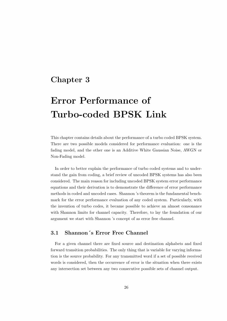
performances in the BER curves. Although among the mentioned algorithms inFigure 3.7 [14], the Max Log MAP and SOVA are adjustable by the introduction ofa linear factor to the end results. Here Lc =1 for the case when the reliability is notknown correctly. The Linear factor is X, which can be used linearly to compensatethe misjudgement of the reliability factor.

X = L/Lc (3.13)

Figure 3.7: Effect of channel reliability factor estimation [14]

It is observed from Figure 3.7, that in the case of a Log MAP based decoder a poorestimate of channel reliability affects the performance badly while for the other twoalgorithms considered it does not make much difference. The reason is the linearityin the Max-Log-MAP and SOVA, according to the discussion carried out in [14]regarding channel reliability. For the former two cases inaccurate estimation onlyintroduce a linear factor X to all the sources of input to the decoder.

On the other hand, Log MAP, there is an additional logarithmic function ofthe form as shown in Equation 3.14, which was introduced as a remedy to theperformance inferiority of the Max-Log-MAP. The function decreases asymptoticallyas the number x is increased in Equation 3.14. Hence the Log MAP algorithm hasa non-linear characteristic which does not allow a poor estimate for the channelreliability factor.


fc = ln(1 + e−x) (3.14)

3.3.2 Fading Channel

In the case of a fading channel, the performance is worse as fading results in largevariations in the signal’s amplitude thus resulting in even higher error rates. Thecoding parameters explained in the previous section have a similar impact on theperformance of turbo-coded systems in the presence of fading channels. Here weconsider only the effects due to the presence of fading in the channel and alsodemonstrate the importance of Channel Side Information, (CSI) for the case of afading channel. In our study we take Rayleigh as an example, which is the mostpopular model for a fading channel.

From Equation 2.5 and Equation 2.6 it can be inferred that the LLR throughthe channel is a product of the matched filter approximated output of the channeldenoted by yk, multiplied by the reliability factor denoted by Lc, and can be givenas,

L(yk|uk) = Lcyk. (3.15)

Since we are concerned with the characterization of fading in a wireless channelfor the reason that it results in a non-uniform SNR profile per code block, therefore,we choose Eb and σ2 to be ’1’ in Equation 2.5, which then changes Equation 3.15into the form shown in Equation 3.16, using a matched filter approximation for yk,

L(yk/uk) = 2a(auk + nk). (3.16)

In the case when there is fading a is a vector, otherwise a = 1 for an AWGNchannel.

Code rate

The effect of code rate is also somewhat the same as we see in the AWGN channeli.e. the smaller is the code rate the better the performance of the Turbo code willbe. Nonetheless, under-performance of curves in Rayleigh fading is pretty muchexpected and can be noticed by comparing Figure 3.5 to Figure 3.8.


Figure 3.8: Performance at different code rates realized by different numbers ofpunctured parity bits [14]

Channel Coherence Bandwidth

It has been observed that the smaller the channel’s coherence bandwidth is thebetter is the performance of a turbo coded system will be till it remains a narrowbandsignal, where the narrow band is a single tap signal for which the signal bandwidth issmaller than the coherence bandwidth of the channel. If BW is the signal bandwidthand Ts is the delay spread between the first and the last path arrival time, whereits reciprocal is called the coherence bandwidth of the channel, then Figure 3.9can be followed to understand the effect of having correlated Rayleigh channelsin comparison to having a fully interleaved or uncorrelated case. Two frequenciesseparated more than the channel coherence bandwidth are uncorrelated.

3.4 Conclusion

This chapter explained those factors which affect the performance of turbo codesin both fading and non-fading channels. It also explains the existing ways of de-picting the performances of coded and uncoded systems, i.e. unlike the uncodedmodulation systems, the error performance ratios for the coded systems are studiedvia simulations. One of the major application, or usage, of the results stored fromthese simulations is in the performance prediction of turbo coded systems used inthe link adaptation techniques. The term performance prediction and its role in link


Figure 3.9: Performance at different degrees of selectivity realized [12]

adaptation shall be explained in detail in the next chapter.

Chapter 4

Performance Prediction and

Fading

The performance prediction of the link is an essential step in modern wireless trans-mitters. An Adaptive Modulation and Coding, (AMC) scheme is an importanttechnique considered in Third Generation, (3G) Mobile Systems [10]. In AMC,performance prediction of the link is based on the Channel Side Information, (CSI).This CSI is actually the Signal to Noise Ratio, (SNR). Normally, the performanceprediction is based on some simulation results which are recorded for a limited num-ber of modulation techniques and code rates. In non-fading conditions the SNR foreach block is definite and constant over the entire code block. Therefore, the perfor-mance prediction works over one to one correspondace for those SNRs against thestored error ratios.

In fading channels the SNR within a code block cannot always be assumed uni-form, as in the case of block fading where the whole code block is faded uniformly.For example, in Orthogonal Frequency Division Multiple Access, (OFDMA), wehave frequency selective fading and in Multiple Input Multiple Output (MIMO),there may be different fading realizations inside a coding block if the code is overmultiple MIMO streams. In this chapter a well known method of evaluating one ef-fective SNR to map for the entire block is explained. Then we present our approachin contrast to the former which considers statistical numbers of the SNR numberseries inside a code block.

38

CHAPTER 4. PERFORMANCE PREDICTION AND FADING 39

4.1 Adaptive Modulation and Coding

In wireless communication systems adapting the signal according to the changingconditions of the channel is among the classical techniques for improving capacityand error performance. This phenomenon of introducing modifications in the signalto follow the variations in the transmitter to receiver link is called link adaptation.There are various kinds of modification which a transmitter makes to adjust thevariations in the channel.

Adaptive transmission methods were first introduced in the era of early seven-ties [9, 16]. Interest in these techniques was ephemeral. With the evolution of tech-nology interest in adaptive modulation methods was revived, as bariers like hardwareconstraints and lack of channel estimation techniques were no longer meaningful. Asa result, many wireless systems, including both GSM and CDMA cellular systems aswell as wireless LANs, are already using, or planning to use, adaptive transmissiontechniques [9].

Two of the well known link adaptation techniques are Power Control, (PC) andAdaptive Modulation and Coding, (AMC). In PC the users at a farther distancefrom the receiver transmit greater power, while those nearby transmit a smalleramount of power. The technique has been used in Code Division Multiple Access(CDMA) systems, to control intracell interference in the uplink. In the downlink thebase station has to divide power among all users and power control in the downlinkis better refered as Adaptive Power Allocation, (APA). In the downlink the idea isto control intercell or intersector interference [2].

In AMC the power of the signal is kept constant. Instead of power, the modulationand coding schemes are changed to cope with the current channel conditions. AMCenables spectrally efficient and robust communication particularly in time varyingchannels. AMC results in an enhanced throughput and efficient communication bysending higher data rates to good channels. As an empirical rule the users closer tothe base station are assigned higher order modulation and high code rates. As theuser moves away from the base station the order of modulation and code rate aredecreased. A diagramatic illustration can be found in Figure 4.1. This switchingdecision is led by a feedback signal from the receiver which is known as the Channelquality Indicator, (CQI) in the scientific literature.


Figure 4.1: Example AMC scheme for a WiMAX base station

The basic premise is the estimation of channel at the receiver and then conveyingthe estimate to the transmitter. Then it is the transmitter which predicts perfor-mance of the current channel for different code rates and, according to the predictiveperformance it adapts the transmission rate. Although in [16] issues like noise, de-lay and bandwidth limitation of the feedback channel are also included as some ofthe real time challenges, but those issues are out of the scope of this work. Althoughmentioned in the same article, [16] issue concerning the restriction of the allowablerates is somehow not that concurrent as with the advent of the modern turbo codesit is possible to attain a wide range of achievable code rates [24].

4.2 Performance Prediction

As from the previous section it can be understood that in order to raise the errorperformance, throughput and spectral efficiency, the modern transmitters are fullybased on performance prediction of the current channel. If all other issues areconsidered to be ideal, i.e. the Channel Side Information, (CSI) is perfectly available,then it becomes essential to have a working mechanism which may predict errorperfomance of the link, based on the CSI, the coding parameters and code rates.


Figure 4.2: Example MCS set

The principle followed is that the better the channel is, the more the data istransmitted to that channel as shown in Figure 4.2. Throughputs for some modu-lation coding schemes are plotted against the SNR. It is observable that there is acontinuous series of intervals with a noticeable optimum MCS corresponding to eachinterval. But following the rule of thumb principle, the selection of MCS is made inconjunction error performance model against the SNR. And the code rate or MCSwith maximum throughput for a given best error performance is chosen. For in-stance in Figure 4.2, between the interval 6.5 and 9 dB, the MCS5 gives the highestthroughput but if this MCS scheme is predicted to give a bad error performancethen the MCS4 appears as the second best choice for the interval mentioned.

A straightforward choice would be to maintain look-up tables which store simu-lation results for a limited number of code rates. Using such a working mechanism,however, is not only restricted to a limited number of code rates but also the selec-tion of code rates in response to particular SNR value is not optimum. In [19, 20] acontinuous function has been proposed which predicts error ratio for any code rateand one of the coding parameter i.e. block length for a turbo-coded system. Alsoin [31], attention has been paid towards the optimum rate quantization for AMCor choice of optimum switching points with in the continuum of Modulation Coding


Schemes, (MCS).

Since there is no analytical relation available in scientific literature which mightexplain the relationship between the error performance and the SNR, therefore thecoded systems are normally studied by undertaking large simulations. Particularly,in [19, 20], continuous mathematical functions have been proposed by fitting modi-fied Sigmoid functions over the simulation results. These mathematical models helpin deciding over the block length and code rate for a user at that instant basedon the SNR known from the feedback signal and the targeted error performance.In [20], the function proposed is a modified Sigmoidal curve and can be given as,

BLER = 1− 11 + eF1(x) + 2eF2(x)

, (4.1)

F1(x) = f(γ,R,B), (4.2)

F2(x) = f(γ,R,B), (4.3)

where γ is the SNR, R is the code rate and B is the block length.

4.3 Fading channel

In a wireless channel the signal is bound to fade because of average distance pathloss, shadowing and diffracting through obstacles and multipath interference. Thisis particularly the case when, due to a fading channel, the magnitude responseis not uniform and hence results in a non-uniform SNR inside a code block. Thisphenomenon brings about a confusion in the SNR mapping to the error performanceratios, considering the Block Error Rate (BLER) in particular.

4.4 Varying SNR and Fading

For wireless channels having a uniform and steadfast SNR level is not realistic.There are always variations in SNR in both time and frequency domains. LargeSNR variations are due to non-uniform signal power which incurs because of sev-eral well explained fading phenomena in scientific literature. Some of the reknownfading phenomena include slow fading which is due to shadowing and diffraction byobstacles between the radio links’ transceivers, fast fading which is because of theinterference between several versions of the same signal displaced on the time scale


and frequency selective fading which is a function of the different frequency responseof the channels as for different frequencies.

Our approach is to characterize this fading in terms of the statistical numbersassociated with a very important link level parameter which is the SNR. The ad-vantage of opting for such a kind of approach towards fading is that it generalizesour performance prediction model for all kind of fading realizations. Especially forthe case of major variations in SNR level, it becomes difficult to map link perfor-mance against SNR particularly when these variations are inside a code block. Tofind a visual illustration of this concept see Figure 4.3.

(a) An example fading signal

(b) SNR variations

Figure 4.3: Non-uniform SNR within a code block

4.4.1 Effective SNR Mapping

One of the approaches is evaluating Effective SNR, which tackles the confusion inthe SNR to BLER mapping arising as a result of the non-uniform SNR value insidethe code block. That effective value is then mapped against the BLER. In [27],five channel models in an increasing order of the doppler shift have been considered.So there are five extents of variation in the SNR inside a block, the method ofmapping has been referred to as Equivalent SNR Mapping, (ESM). Mathematically,the effective SNR for the case when the channel does not have a uniform state insidea code block is given as,

γeff = I−1(∫I(γ)fSNR(γ)dγ) (4.4)

γeff = I−1(∑i

I(γi)pi), (4.5)


Figure 4.4: A comparison among different information measures [27]

where, fSNR(γ) in Equation 4.4 is the probability density function for the contin-uous valued channel symbol SNR γ, and pi in Equation 4.5 is the probability massfunction for the discrete valued SNR γi. I(γ) is introduced as a new term calledInformation measure, which actually characterizes the channel capacity. There aremany different ways to define the information measure. It can be defined as mu-tual information, linear SNR, a logarithmic function of SNR, as a cut off rate for aspecific kind of modulation, and as the channel capacity of the AWGN channel.

In Figure 4.4 it can be observed that the mutual information has a Sigmoidalform. And for a given modulation format, the amount of information that a channelcan pass should follow a Sigmoidal curve. As SNR increases, the convex form ofthe curve overestimates the information that can be transfered. Therefore, theSigmoidal property is essential for the information measure, in particular for systemoperating close to channel capacity, i.e. Turbo codes.

4.4.2 Performance prediction Model for Fading Channels

In the light of the discussion in the previous section it can be appreciated that largescale variations in the SNR or state of channel within a coding block need specialtreatment for understanding the system performance. Therefore, it can be statedthat the models presented in [19] and [20], for link performance prediction are notoptimal for large variations, or in other words, for the fading channels.

It is known that in fading channels the magnitude response of the channel mayvary either in an uncorrelated or correlated fashion. Under any circumstances, how-


ever, the statistical treatment is always possible for different SNR values assumedinside a code block, i.e. the mean and variance for those SNR numbers can alwaysbe evaluated. Also in [27] it can be found that for a linear average as informationmeasure, the performance curves were unique for each extent of variations in thechannel. Figure 4.5presents a comparison of this. Although, with mutual informa-tion the performance curves are found almost variations independent. Therefore, itis required to have more than one statistical number to define the error performance.

(a) Mutual Information as Information Measure

(b) Linear average as Information Measure

Figure 4.5: Error performance comparison for two different information mea-sures [27]


Code rate is an essential parameter, as a rule of thumb for good channels MCSsof high code rates and high order modulation schemes are preferred. From thatperspective, the code rate is a very important parameter from a resource allocationperspective as the user in close proximity to the base station enjoys higher datarate. In [19, 20] also one of the parameter considered is the code rate.

In order to make a model precise for fading channels, it is also needed to introducesuch a parameter in the model which takes care of the channel conditions.From theprevious section we know that the average value of SNR numbers inside a codeblock is not on its own enough to describe the performance of the coded system,specifically for large SNR variations or fading channels. Therefore, the variance ofthe SNR numbers is the parameter that should be taken care of when the case ofcoded systems is modeled for fading channels.

4.5 Conclusion

In this chapter the phenomenon of performance prediction and its application inthe AMC implemented systems was discussed. Moreover, the problem of large vari-ations in the SNR values with a code block was discussed. In the discussion aboutthe Equivalent SNR Mapping methods in [27] it was found that the linear averagingmethod of ESM is the worst. And in [27], it was stated that the first order statisticsof SNR are not sufficient because then performance becomes model dependent and,as a straightforward strategy, extensive simulations would be required to charac-terize the performance. In the next chapter our approach for studying, modelingand simulating a turbo-coded link, which experiences a non-uniform channel stateinside the code block, has been explained. In this approach the fading has beencharacterized according to the mean and variance of the SNR number series insidea code block.

Chapter 5

Link Simulations

This chapter outlines the entire link along with some details about the simulationactivity undertaken, which is designed to imitate the targeted link features for in-vestigation. The principle adopted to model the channel has also been explained.The unique model for the channel has been described with fair mathematical treat-ment. Along with channel in this chapter several details about the simulation issuesare also presented. A comparative discussion of the methodology developed in ourwork with an alternative technique to define performance of coded links in fadingchannels is an important part of this chapter. In the end the performance curves ofthe considered turbo link obtained from simulations, are presented and analyzed.

5.1 Link Layout

There are three known ways to evaluate the performance of a communication sys-tem: calculations with the formulas relating system parameters with performance,waveform-level or link-level simulations and measurements with hardware proto-types [17]. Unfortunately, it is often impossible to evaluate the performance ofcomplex communication systems using analytical techniques. At the other extremehardware prototyping is the most accurate and credible method but it is very costly,time-consuming and an inflexible method.

Simulation-based analysis is more manageable. This is particularly so with theconcept of a hierarchical view of a simulation setup where the possible computa-tional load can be very efficiently distributed. Accoring to [17], there are three tiersof the hierarchy, i.e. network tier, link tier and implementation tier. Network tiersimulation is rendered to validate and study system performance for given specifi-

47

CHAPTER 5. LINK SIMULATIONS 48

Figure 5.1: Block diagram of the overall Link

cations of the communication links. Link tier simulation is undertaken to verify thespecifications of those communication links. And implementation tier is simulatedto cater for the implementation related issues of the blocks, for example, filters,modulators, encoders and amplifiers constituting those radio links.

Communication links are all about the transmission of waveforms over differenttypes of communication channels (free space, cables, optical fibers, etc.) Thesewaveforms are actually information-carriers. In digital communication systems, theperformance of communication links is measured in terms of error performance ra-tios, like Block Errror Rate, (BLER) and Bit Error Rate, (BER). These ratios areestimated by simulating the flow of waveforms using models for functional blockssuch as modulators, encoders, channels and amplifiers, among other things.

The turbo-coded BPSK Link under discussion is meant to consider turbo encodingand Binary Phase Shift Keying, (BPSK) modulation of interleaved bits. Then theother end of the link is supposed to depict the demodulation and decoding step.In order to cover the effects due to a wireless fading channel, a suitable channelis modelled for which the corresponding statistical numbers of the supposed SNRdistribution inside the code block, are known and manipulatable to alter the channelcoefficients. Figure 5.1 can be followed to see the overall link layout.

As a part of the simulator a comparison logic is embeded to undertake the cal-culations for BLER and BER. The channel side information is assumed to be fully


Figure 5.2: PDF of a two-peak distribution: p=0.5,m1=-10,m2=5,v1=1,v2=3

available. The ready-made turbo encoder and decoder used in the simulator areUniversal Mobile Telecommunication System, (UMTS) standards compliant. A de-tailed discussion over the simulator, simulation results and analysis on the obtainedperformance graphs can be followed in the next chapter.

5.2 Two-peak Distribution

Mapping link performance in terms of error ratios like Block Error Rate (BLER) orBit Error Rate (BER) against SNR becomes vague when within a code block thereare many SNR values, which may be even bit-specific. In our approach we representthis SNR number series per code block as a distribution, which is a weighted sumof two normal distributions. We call this distribution a two-peak distribution.

The distribution proposed is a sum of two normal distributions in such a way thatthese two distributions are weighted by a fractional parameter denoted by p. Thevalue of p is allowed to vary from ’0’ to ’1’. Other than this there are four otherparameters which altogether generate numbers out of this two-peak distribution.The other parameters are the mean of the first normal distribution denoted by m1,the variance of the first normal distribution denoted by v1, similarly, m2 is themean of the second normal distribution and v2 is the variance of the second normaldistribution. Mathematically, the Probability density function, PDF can be seen inEquation 5.1 and a graphical demonstration of the PDF can be found in Figure 5.2.

PDF =e− (−m1+x)2

2v1 (1− p)√2π√v1

+e− (−m2+x)2

2v2 p√2π√v2

(5.1)


From a quick inspection of the PDF graph it can be inferred that the distributioncan be related to the higher order statistical numbers of the SNR distribution byplaying with the five parameters of the two-peak distribution. For instance, the meanof the overall distribution can be adjusted by changing individual means m1,m2and the parameter p. Similarly, for variance of the overall distribution, individualvariances also become important.

Some other higher order statistics like Skewness and Kurtosis are also control-lable by this distribution. Since Skewness is defined as the measure of balance orskew in a population sample, here parameter p can be used to manage the skew inthe SNR distribution. In the same way kurtosis is the measure of peakedness inthe data set. This peakedness in particular can be altered by changing individualvariances. Moreover, extreme values of p result in a rise in the peakedness of thedata set. Mathematical derivation to solve all four statistical numbers in terms ofthe mentioned five parameters can be found in the appendix to this thesis.

5.2.1 Mean and Variance Expressions

The focus of this thesis work is limited to only two statistical numbers, i.e. themean and variance of the SNR distribution. As a first step we evaluate the meanand variance of the two-peak distribution in terms of the constituent parameters,i.e. p,m1,m2, v1, v2. As by definition we know the mean, m can be given by,

m =∫ ∞−∞

xPDF (p,m1,m2, v1, v2)dx (5.2)

Similarly the variance, v of the SNR distribution can be expressed as,

v =∫ ∞−∞

(x−m)2PDF (p,m1,m2, v1, v2)dx (5.3)

The PDF taken is the one from Equation 5.1 and has also been plotted for anexample case in Figure 5.2. The resulting expressions of m and v in terms of theparameters, p,m1,m2, v1, v2, which were obtained after solving the integrals fromEquations 5.2 and 5.3 are obtained as,

m = m1 −m1p+m2p (5.4)

v = −(−1 + p)((m1 −m2)2p+ v1) + pv2 (5.5)


5.2.2 Channel Coefficients

The channel coefficients are generated randomly, for an intended set of the statisticalnumbers, i.e. m and v. The larger the size of the randomly generated sample of SNRnumbers for one code block, or longer the block length is, the closer the statisticalproperties of the numbers are to the intended set of statistical numbers. Also, thedifference between the intended statistical numbers, i.e. m and v and the statisticalproperties of the numbers generated, is random and changes every time. Usually,the evaluation of error performance ratios is averaged over a very large numberof shots in order to get a more reliable value which is supposed to be very closeto the intended statistical values. Such simulation types are called Monte Carlosimulations, [17] pg.15.

The values of m and v are considered in the dB domain, as are the SNR numbersgenerated. Since the SNR is a ratio of the signal power to the noise power, thereforeif M is the signal magnitude, a is the channel amplitude response, N0

2 is the noisespectral density, which is also equal to noise variance σ2 [21] and BW is the signalbandwidth. Mathematically, it can then be given as,

γ =(aM)2N02 BW

(5.6)

For our simulations, since we intend to characterize the effects of fading, thenoise variance is therefore taken to be constant and unity for ease. Also we takebandwidth to be unity. Moreover, the signal power for a BPSK modulated signal isunity. Therefore, from Equation 5.6 the channel coefficients for the fading channelcan be calculated as,

a =√γ (5.7)

5.3 Simulator Structure

The simulator is supposed to depict a complete scenario of the link layout as dis-cussed in Section 5.1. In order to undertake the simulations for a turbo coded BPSKlink in a fading channel, a ready-made turbo encoder and decoder have been used.These are versatile enough to accomodate a continuous series of code rates andblock lengths, and are configurable for almost all kinds of generator polynomials.In our research, the target generator polynomial is UMTS compliant i.e. (13, 15)8.


Figure 5.3: Block diagram of the simulator

A visual elucidation of the the entire simulator is presented as a block diagram inFigure 5.3.

From block diagram it can be seen that a comparison logic has been embedded toevaluate the BLER and BER. The evaluation of these ratios, i.e. the BLER andBER is not a function of just one occurence rather a loop for N numbers of timeruns which stops till some pre-set number of blocks in error is achieved. N is a largenumber, for example, the number of times this loop runs is a thousand times of thenumber of blocks in error if the BLER is targeted to be 10−3. And a recommendedchoice for blocks in error is 100, if stable and reliable results are required.

Each round of the loop is comprised of: the generation of some data bits, randominterleaving of those data bits, encoding via a turbo encoder, then matched filterapproximation based multiplication with the instantly generated channel coefficientsusing two-peak distribution (generating numbers for a desired mean and variance ofthe distribution), accompanied by the addition of some gaussian noise, and, finally,log MAP decoding (as explained in Section 2.4.4). After decoding, the comparisonlogic updates the total number of bits in error and blocks in error, the ratios, i.e.BLER and BER, are evaluated after the division of these by the N .


Figure 5.4: Unreliable curves obtained in first attempt

5.4 Simulation Issues

The channel model has been designed so that it favours the characterization of thechannel fading in terms of the statistics of the SNR profile within a code block. Theexpressions in Equations 5.4 and 5.5 are the mean and variance of the SNR in termsof the five parameters of two-peak distribution, which are solved together and usingrandom numbers in a trial and error fashion which was a time-consuming process.Moreover, turbo decoding also consumes a considerable amount of computationalresources. Therefore, to make simulations more manageable, the task was dividedinto two subtasks.

As a first task we stored one set of parameters of two-peak distribution, i.e.m1,m2, v1, v2, p, against each desired combination of the mean and variance of theSNR profile. While in the second step we used the prestored parametric values foreach combination of the mean and variance. The channel coefficients were generatedfor just one set of parameters for a specific mean and variance combination. Theresulting plots obtained using this approach were not reliable. A sample of thosecurves can be seen in Figure 5.4.

The reason behind this unwanted behaviour was because of the fact that everycombination of mean, m, and variance, v, was specified to just one parametric setof m1,m2, v1, v2, p. There, in fact, we just associate each value of m and v toone particular parametric set and also for any two combinations of m and v theircorresponding parametric sets are unrelated while we plot them as a single curve.The phenomenon of being unrelated can be explained as having different higherorder statistical numbers like skewness and kurtosis. This scheme does not ensurehigher statistics to be the same for each combination of mean and variance of theSNR profile inside a code block.


Figure 5.5: Smoother curves with scaling problem

5.4.1 1000 snapshots approach and smoothness in performance curves

The problem discussed in the previous section demands some assurance of havingconstant higher statistics or any other lurking variables of the two-peak distributionfrom each parametric set. An easier way is to have multiple parametric sets of two-peak distribution converging for the same values of mean and variance of the SNRprofile. Such that the resulting BER/BLER obtained shall be averaged over thosemultiple snap shots of the two-peak distribution.

But generating multiple parametric sets for each combination of m and v is ahuge target to achieve. Moreover, the number of snapshots should also be highenough so that a wider span of snapshots for averaging shall yield a more genericchannel model, which does not have an association restricted to a small number ofsnapshots. Therefore, 1000 is chosen to be a reasonable number for snapshots.

In our simulations, we generate 1000 snapshots or parametric sets, ofm1,m2, v1, v2, p

for m = −2dB and v = 20dB. In order to ensure that we have the same higher orderstatistics or lurking variables for every combination of mean and variance, we changethe mean and variance of the generated SNR profile mathematically, i.e. by addingthe factor meandesired − meancurrent to each of the number of any number serieschanges current mean to the desired mean. Similarly, the factor

√variancedesiredvariancecurrent

ismultiplied with each number of the number series. Manipulating, a higher order sta-tistical number like variance changes the mean also but the reverse is not true. Thecurves obtained using this technique resulted in smooth curves. The plots obtainedcan be found in Figure 5.5.

Although the curves obtained were smooth, the pattern followed, however, was


exactly the reverse of the expected one. For higher variance in the SNR profile theperformance of the link improves. The reason was traced by evaluating the SNRlinearly and it was found that for a 1 dB rise in variance there was a 0.1 dB rise inthe SNR. For example, for v = 5dB if m = −2dB then the corresponding linearlyevaluated SNR value represented in the dB domain was 0.5 dB higher i.e. -1.5 dB.Therefore,there appears a dB shift of 0.5 dB towards left in the whole curve forv = 5dBbecause by selecting a wrong axis it plots the BLER for -1.5 dB against -2dB. Accordingly, the same shift is of 1 dB approximately for a curve having v=10dB.

5.4.2 Linear average dB represented SNR on x-axis

In order to attain a reliable trend from our analysis in the previous section it can beinferred that the performance curve should be plotted against the linearly evaluatedmean of the SNR profile which is represented in the dB domain. With this correc-tion the curves obtained were smooth and also the trend obtained is closer to thetheoretical principles. The BER and BLER curves obtained for various variancescan found in Figure 5.6.

5.4.3 Curves for UMTS standard Turbo code in fading channels

The curves shown in Figure 5.6 were plotted to undertake the validation task asthe curves referred to in [14] were plotted for a generator matrix (7, 5)8. After vali-dating the simulator setings, the same channel was simulated with UMTS standardcompliant turbo codes, i.e. the generator matrix we considered for the simulator is(13, 15)8. The performance of the link has been considered for various code ratesalong with different variances. A complete picture of the Turbo code performancecurves for various code rates and variances can be found in Figure 5.7.

5.4.4 Results Analysis

The long haul simulations talked about helped obtaining smooth curves relatingBlock Error Rate to linear mean values of the SNR profile inside a code block in dBreceived at the decoder. Each individual curve can be characterized for a definitevariance of the SNR profile inside a code block and code rate of the turbo code used.It can be noticed that each bunch of several consecutive curves of unique spacing issupposed to have a common rate, whereas inside each equi-spaced curves bunch theSNR variance for each curve is different.


(a) Block Error Rate Vs linear mean SNR in dB

(b) Bit Error Rate vs linear mean SNR in dB

Figure 5.6: Plots with linear mean SNR in dB on x-axis

Another noticeable phenomenon is the dependence of the spacing between twoconsecutive curves in each bunch over the code rate. Therefore, it can be inferredthat SNR variance has an adverse effect on the link performance and this effectworsens for higher code rates. From Figure 5.7 it can be observed that the coderate of the turbo code just operates as a linear shift function. Similarly, withinone particular bunch of curves having a common code rate, the change in the SNRvariance is also a linear shift operation, although the amount of this shift operationis code rate specific. In the next chapter a mathematical model has been proposedwhich is obtained by curve fitting a modified version of sigmoidal function over thesimulation results.


Figure 5.7: UMTS standard compliant curves for various code rates


5.5 SNR statistics vs Effective SNR value

In [27] several methods of averaging have been suggested and the best one forturbo-coded systems is of mutual information averaging. There is no exact relationto evaluate mutual information from the Channel Side Information to obtain aneffective SNR value. The approximate formula selected in [27] for the evaluation ofeffective SNR is complex, involving cubical and quadratic polynomials along withexponentials. Therefore, given in practical systems the method is prone to errors.

Contrary to that, embarking on the path towards the SNR statistics is practicallymore feasible as representing the entire SNR distribution with two statistical num-bers makes it much more favourable for practical consideration. Moreover, in [27],it says for linear averaging the performance is channel model dependent, but in ourcase only statistical numbers are the criteria to predict performance, so it somehowbecomes independent of the type of the channel model considered.

The mean value of the SNR distribution is the linear average. In our technique,we have an additional statistical number, i.e. variance, which is specific for eachcurve if the BLER is plotted against the mean value of the SNR distribution. Suchplots are the results of our simulations, which were performed for various code ratesand shall be discussed in detail in the next chapter.

In order to have a fair comparison, however, it is required to tune some commonchannels for both methods. This is because the channels used in [27], are strawmanchannels which are characterized for different doppler speeds. Contrary to that inthis thesis we have used a two-peak gaussian distribution and realized it for differentsets of mean and variance of the dB SNR profile inside a code block.

5.6 Conclusion

This chapter was intended to develop a comprehensive understanding of the chan-nel model proposed and the simulation activity pursued to achieve the resultingperformance curves trends. The channel model was found well-tuned to suit theinvestigations to the study effects of statistical numbers like mean and variance ofcode block SNR numbers in defining the performance of turbo-coded links in fadingchannels. Moreover, it can be noticed that while modelling for two statistical num-bers it is important to have the same high order statistics for all the iterations used


for averaging in order to avoid strange scatter in the simulation performance curves.Also, it was observed that although we manipulate the mean and variance in the dBdomain for the SNR numbers inside code block, but to plot the performance curvesit is the linearly calculated averaged SNR value, taken on to x-axis, which gavereliable and theoretically comprehendable curves. In the next chapter we proposea mathematical model to fit the curves obtained through the described simulationsin the current chapter.

Chapter 6

Curve Fitting

A modified version of Sigmoid function has been fitted over the simulation resultsover a semilog plot. The points obtained from simulation tend to form performancecurves for turbo-coded links. The curve fitting done in this regard results in a con-tinuous mathematical model, which can be used to evaluate the performance of thelink. In this chapter, the steps involved in maturing a simple Sigmoid function intoa comprehensive mathematical model are explained in detail. Firstly, the possiblekind of modifications in the Sigmoid function are described. Secondly some of theBLER vs mean SNR curves have been fitted with some modified versions. Further-more, in order to understand the nature of the relationship between the code rateand the variance of the SNR, constant BLER surfaces have been formed. In thefinal step a proposed function comprising of three independent variables i.e. meanof SNRs in dB m, variance of SNRs in dB v and code rate R has been fitted and op-timized to achieve the optimal fitting metric. The fitting metric has been redefinedto suit semilog plots.

6.1 Heuristic selection of a Sigmoid function

There are many ways to do curve fitting over the previously known data. Fittingpolynomial curves is the most popular choice. But often the biggest problem facedis the tendency of a polynomial fit to oscillate about the data points. An illustrationof such a tendency can be found in Figure 6.1.

Another approach is based on the heuristic selection of any conventional functionand then modifying it to cover the data points. The curves in Figure 5.7 are closestto the Sigmoid function. The mathematical form of a simple Sigmoid function canbe given as,

60

CHAPTER 6. CURVE FITTING 61

Figure 6.1: Oscillating polynomial fit over some data points

Figure 6.2: An example Sigmoid curve

F (x) =1

1 + e−c1x−c2. (6.1)

6.2 Modifications in Sigmoid function

The Sigmoid function considered in 6.1 can be plotted as shown in Figure 6.2.However a function closer to the performance curves can be given as in Equation 6.2.The diagramatic representation of the function in Equation 6.2 can be found inFigure 6.3.

F (x) = 1− 11 + e−c1x−c2

(6.2)

Looking at the multitude of slopes, slightly floored edges and unique positioning


Figure 6.3: A closer Sigmoid curve

Figure 6.4: Sigmoid curves of different slopes

of each curve in the simulation curves in Fig 5.7, the neccessity of introducing somemechanics to vary the slope and flooring of the Sigmoid in Figure 6.3 becomesevident. In the light of the results found in [19, 20] we enlist two such mechanisms.

6.2.1 G-factor

Among the manipulable mechanics of a Sigmoid slope is an important parameter.The modified form of the Sigmoid with the G-factor can be given as,

F (x) = 1−(

11 + e−c1x−c2

)G(6.3)

An example plot can be seen in Figure 6.4, which shows the change in the slopewith the change in the values of the parameter G in a linear plot. It clearly shows


Figure 6.5: Sigmoid curves for changing G in a semilog plot

that the slope of the Sigmoid has a direct relation with the value of G for a linearplot. On the other hand, in a semilog plot, the G parameter helps changing theposition in the reference of the logarithmic y-axis without affecting the asymptoticslope of the curve. This effect is noticeable in Figure 6.5.

From a brief observation of the curves in Figure 5.7 it can be noticed that allthe BLER vs mean SNR curves have almost same slopes, and these curves can berepresented as the SNR variance and code rate depending linearly shifted versions ofeach other. This all means that the G-value presence does not have a very significantrole to play in the curve fitting of the discussed curves.

6.2.2 Flooring Effect

Sigmoid is the most suitable curve to fit over the obtained results, but the semilogplot of a Sigmoid function have an asymptotic straight line slope or a smooth roll off.On the other hand the curves shown in Figure 5.7 have a sort of flooring tendencyand they do not roll off as straight as a Sigmoid function on a semilog plot.

To understand the flooring concept we need to understand the Sigmoid functionin a different way. Consider the parameters a and b in Equation 6.4.

F (x) = 1− 11 + e−a

′ (x−b′ )(6.4)

The value of a decides the slope of the Sigmoid and b determines the position ofthe bending point or knee point of the Sigmoid in a semilog plot. Example plots


Figure 6.6: Sigmoid curves for a known slope and position

Figure 6.7: Sigmoid curves with different levels of flooring effect

can be found in Figure 6.6.The red dots marked in the figure are the bending points or knee points of the Sig-

moid in a semilog plot. In order to introduce a flooring effect in a Sigmoid curve, oneshould have two exponentials instead of just one. The additional exponential shouldhave a lower a and lower b. Let a1,b1 and a2,b2 be the slope and position controllingparameters of the first exponential and the additional exponential for a Sigmoidfunction. Then to see different examples of Sigmoids with flooring, Figure 6.7 canbe followed. The mathematical demonstration can be given as,

F (x) = 1− 11 + e−a1(x−b1) + e−a2(x−b2)

(6.5)


Figure 6.8: Constant BLER surfaces

6.3 Cross Relationship between Code Rate and SNR

Variance

A brief look at Figure 5.7 reveals the fact that for each bunch of four curves there isa uniform spacing which is due to SNR variance for each bunch there is a constantcode rate. In other words effects of SNR variance are worse for a higher code rate.Now to understand the degree of relationship between the two mentioned variables,constant BLER surfaces have been considered and MATLAB sftool was used to fixsurfaces over the considered points. The best fit was obtained with the form shownin Equation 6.6. A pictorial demonstration of two constant BLER surfaces can befound in Figure 6.8,

F (v,R) = c1Rv + c2R+ c3v + c4, (6.6)

where R represents the code rate, v is the SNR variance and c1,c2,c3, and c4 arethe fitting parameters.

6.4 Proposed Function

The selected base function been used for curve fitting over the obtained simulationresults is a Sigmoid function. Although to adjust a Sigmoid over the simulationresults its positioning and slope are manipulatable. In the considered simulationresults in Figure 5.7 there is a need to introduce one additional exponential in theSigmoid-based function for Flooring. Considering the arguements presented in the


previous sections the fitting function we propose can be given as,

Pe(m, v,R) = 1− 1(1 + eF1(m,v,R) + eF2(m,v,R) + eF3(m,v,R))G

. (6.7)

Where, G = k22 and F1(m, v,R), F2(m, v,R) and F3(m, v,R) can be given as,

F1(m, v,R) = k1.m3 + k2.m

2 + k3.m+ k4.v + k5.R+ k6.R.v + k7, (6.8)

F2(m, v,R) = k8.m3 + k9.m

2 + k10.m+ k11.v + k12.R+ k13.R.v + k14, (6.9)

F3(m, v,R) = k15.m3 + k16.m

2 + k17.m+ k18.v + k19.R+ k20.R.v + k21. (6.10)

6.5 About Fitting Method

To fit the proposed function over the simulation results a non-linear curve fittingalgorithm is used, which is conveniently usable in the form of a MATLAB commandlsqcurvefit. The reason for selection of this command is due to the fact thatthe proposed function is a Sigmoid function, which is a non-linear function. Thedefault optimization method been used by this command is Trust Region ReflectiveOptimization, which is explained in [7].

In [7] the optimization is explained as a reflected ray inside a trust region, whenthis ray meets a local minimizer then it is unneccessary to reflect any more. Thisphenomenon might affect the optimality of the fitting coefficients obtained in theresult of the command, lsqcurvefit, running once. In order to avoid this situationwe undertake an exhaustive search with 8000 shots and among these we store theone which yields the least value for the fitting metric. The fitting metric is definedin Equation 6.11.

6.5.1 Fitting Metric

Some of the traditionally well-known curve fitting metrics include: R-square, RootMean Square Error (RMSE) and Sum of Square Error (SSE). For semilog and log-arithmic plots these metrics are not expected to ensure proper fitting. Dealing


with a similar problem in [20] a modified form has been used, the one presented inEquation 6.11 is altered as per our requirement of having the variance of SNR dBnumbers instead of block length which was there in [20].

Fittingmetric =∑i,j,l

(log10(BLERsim(Ri, vj ,ml)))− (log10(BLERfit(Ri, vj ,ml)))2

(6.11)

6.6 Optimal Form of the Function

The form of the fitting function presented in Equation 6.7 requires 22 parameters,to fit the simulation results, although the presented form is subjected to optimiza-tion. In [20] an exhaustive search over parameters has been carried out whichindiscriminatingly takes every combination into account. For instance, one examplecombination could be if all 22 parameters are used. Similarly, if first 11 are usedkeeping rest be unused or all even numbered parameters are used while keeping restunused can be other example combinations.

In the light of pre analysis it would be redundant to search for every combinationof these 22 parameters. For instance, in [20] the fitting metric has been evaluatedeven for the case when only 1 or 2 fitting parameters are used and the rest areunused, which gave the fitting metric in several thousands. Similarly, it also countsup those combinations in which one or two or all the three independent variables(i.e. R, v and m) are not present, which again is an example of a redundant searchbecause such cases can never be optimal.

Therefore, we categorize the sets of parameters as twelve meaningful and logicalcombinations. An investigative search is carried out for these cases. Then on thebasis of the obtained results an optimal approach has been decided. Those twelvecases and the resulting fitting metrics along with the values assigned for the termsused can be found in Tables 6.2 and 6.3. In the first six cases the G-factor is dropped,while in the remaining six the G-factor is also used.

In each of these six cases three are with enhanced error flooring, such that theyhave two additional exponentials instead of just one as it was in [20], and onlythesame one additional exponential we have for the case of without enhanced errorflooring. Then in each of the three out of total four triplets, we have the Linear,


quadratic and Cubic polynomial of m, which is the mean SNR value. The tabularexplanation can be found in Table 6.1.

Table 6.1: Explanation of each Case

Case Explanation

1 Linear polynomial

2 Quadratic polynomial

3 Cubic polynomial

4 Linear polynomial + enhanced flooring

5 Quadratic polynomial + enhanced flooring

6 Cubic polynomial + enhanced flooring

7 Linear polynomial + G-factor

8 Quadratic polynomial + G-factor

9 Cubic polynomial + G-factor

10 Linear polynomial + enhanced flooring + G-factor

11 Quadratic polynomial + enhanced flooring + G-factor

12 Cubic polynomial + enhanced flooring + G-factor

6.7 Conclusion

From Tables 6.2 and 6.3 it can be observed that inclusion of the G-factor worsensthe fitting metric. Although by having three exponentials in the Sigmoid functionthe improvement in metric is evident. Case 6, which is for a cubical polynomial givesthe best fit but requires 21 parameters for its description. The overall computationalload has a dependency over the frequency of the usage of the model also, which isapplication specific. Alternatively, it can be stated in a straightforward manner thatthe more the number of parameters is, the greater the computational burden shalbe.

However, on the other hand, the lower the number of parameters is, lower thelevel of accuracy of the model shall be, which has an impact on the accuracy ofthe overall system level simulation. This implies selection of a particular modelshould be a trade-off between the required accuracy and consideration of the possible


Table 6.2: Parametric values and correpsonding Fitting metric for cases withoutG-factor

kj case#1 case#2 case#3 case#4 case#5 case#6

1 - - 0.0105 - - -0.028

2 - 0.0165 -0.2874 - -0.2 0.1357

3 5.667 -3.654 -4.314 -4.573 -4.682 1.8

4 0.666 -0.0374 -0.543 -0.1051 -0.576 -0.363

5 -19.587 48.061 66.193 62.465 68.972 1.966

6 -1.7827 0.866 1.966 1.079 2.02 0.6019

7 -24.286 -22.407 -29.819 -28.167 -31.1 -17.956

8 - - -0.006 - - -0.015

9 - -0.199 0.067 - -2.92 0.075

10 -4.008 -4.795 -3.756 -1.028 4.872 -3.653

11 -0.088 -0.475 -0.0312 -5.552 -1.65 -0.148

12 54.31 70.421 48.099 -12.27 20.535 47.379

13 0.9671 1.8906 0.8613 -5.687 4.337 1.055

14 -24.379 -31.746 -22.5613 -32.151 -16.94 -22.161

15 - - - - - 0.0536

16 - - - - 0.0224 -0.37

17 - - - -3.038 -3.748 -4.69

18 - - - -0.0046 -0.029 -0.084

19 - - - 40.1188 49.124 69.81

20 - - - 0.7497 0.8635 1.146

21 - - - -20.231 -22.883 -31.428

22 - - - - - -

Fitting metric 1.9789 1.5706 1.5197 1.7745 1.2232 0.9571

computational load due to any specific number of parameters for a system-levelsimulation.


Table 6.3: Parametric values and correpsonding Fitting metric for cases with G-factor

kj case#7 case#8 case#9 case#10 case#11 case#12

1 - - 0.016 - - 0.02

2 - -0.104 -0.125 - 0.029 -0.1698

3 -3.923 -2.372 -3.84 -3.946 -3.7 -5.456

4 -0.07 -8.28 -0.136 -0.0714 -0.008 -0.236

5 53.36 38.626 53.33 53.774 48.52 75.483

6 0.925 13.27 1.0547 0.922 0.826 1.556

7 -24.324 -20.427 -24.1 -24.494 -22.998 -33.36

8 - - -0.054 - - -0.213

9 - -0.097 0.72 - -29.967 -0.88

10 -6.467 -3.82 0.11 3.555 2.418 -10.45

11 -9.68 -0.122 -9.28 -6.136 -2.169 -77.17

12 89.35 53.6 5.83 -22.688 -3.85 183.432

13 -25.95 1.036 13.5 -4.34 -1.76 -42.73

14 -43.09 -24.26 -23.7 -24.56 -34.4 -86.506

15 - - - - - 0.0139

16 - - - - -0.166 -0.1056

17 - - - 3.66 -4.35 -3.2

18 - - - 1.367 -0.4 -0.04

19 - - - -18.83 63.2 45.1188

20 - - - -2.37 1.664 0.7943

21 - - - -15.83 -28.5 -21.003

22 1.2304 1.3429 1.3955 1.268 1.0815 0.7647

Fitting metric 2.398 3.549 1.7911 1.64 1.375 1.394

The last six models are not considerable because of the fact that they require anadditional parameter and are inferior in fitting as well. A pictorial demonstration ofthe fitting of Case 6 over the simulation curves shown in Figure 5.7 can be observed


Figure 6.9: Case 6: Fitting the simulated curves with 21 parameters

in Figure 6.9.The constructed model is a continuous function for variance of the SNR profile

inside a code block and Modulation Coding Scheme, (MCS) code rate. The modelcan be used in place of the look-up tables and can be used in system-level optimiza-tion, particularly with differentiation-based analytical optimization methods. Oneessential point of this model is the versatility of its usage for all kinds of fadingchannels. This is because it characterizes fading in terms of the variation in SNRdB value within a code block incuring due to the fading phenomena in a wirelesschannel.

To understand how different this model is in comparison with the models proposedin [19] and [20], we take AWGN models for a case when we want to know the trans-mission SNR. The transmission SNR is preddicted on the basis of the performanceprediction model. For instance, if we want to attain BLER performance around0.01. Moreover,if there is a compulsion to choose code rate being 2/3, which might


be compulsory for some targetted data rate. And it is assumed that the variance inthe SNR values inside each code block is 15 dB.

Here the old AWGN channel-based model shall propose 4 dB for SNR, which isthe case for SNR variance being zero i.e. AWGN case. Now, considering Figure 6.9to see the model while to recognize the curve for v = 15 dB for code rate being2/3 refer to Figure 5.7, it suggests mean SNR to be 6.25 dB for SNR varianceequal to 15 dB. In fact BLER value is 1 for a mean SNR equal to 4 dB if SNRvariance is 15 dB, which means there shall be no transmission effectively if oldAWGN based performance prediction model was used for performance evaluationprior to transmission.

6.8 Prospective Development

As a future work it is essential to undertake a fair comparison of this method withthe Effective SNR Mapping (ESM) method. A fair comparison requires applicationof both of the predictors on such a channel for which both of the channels area sub-set, i.e. the one considered in [27] and the two-peak distribution channelconsidered in this dissertation. Another way would be to evaluate effective SNRvalues for each channel realization of two-peak distribution for each combination ofmean and variance of the SNR profile. And a further area of investigation could beto determine the corresponding BLER values using an AWGN prediction modelas presented in [20] to compare with the BLER simulation results.

It is also decidable on the basis of a comparison between the predictor based onESM vs the one based on the mean and variance of the SNR profile modelling, thatwhether the two statistical numbers used are good enough or whether there is a needto go for an investigation with higher order statistics. A method for determiningparametric values p,m1,m2, v1 and v2 as discussed in Chapter 5 for a given set ofmean, variance, skewness and kurtosis of the SNR value profile inside a code blockcan be found in Appendix A.

Appendix A

Parametric Expressions for Four

Statistical Numbers

In this appendix we present a solution to yield expressions for the parameters of two-peak distribution i.e. p,m1,m2, v1 and v2 in terms of first four statistical numbersof the SNR profile inside a code block. These four statistical numbers are mean,variance, skewness and kurtosis. The Probability Density Function, PDF of a Two-peak distribution is given as in Equation 5.1. The expressions for the mean andvariance can be found in Equations 5.2 and 5.3. After solving the integrals inEquations 5.2 and 5.3 the expressions found for the mean and variance of the SNRprofile within a code block are given as in Equations 5.4 and 5.5.

The integral expressions for skewness and kurtosis can be given as,

S =∫ ∞−∞

(x−m)3PDF (p,m1,m2, v1, v2)dx, (A.1)

K =∫ ∞−∞

(x−m)4PDF (p,m1,m2, v1, v2)dx. (A.2)

The expression found after solving the two integrals can be simplified as,

S =−m3 −m3

1.(−1 + p) + 3.m21.m.(−1 + p) + 3.m2.m

2.p

v3/2

−3.m1.(−1 + p).(m2 + v1)v3/2

+m2p.(m22 + 3.v2)− 3.m.(v1 + p.(m2

2 − v1 + v2))v3/2

73

APPENDIX A. PARAMETRIC EXPRESSIONS FOR FOUR STATISTICAL NUMBERS74

(A.3)

K = −3 +m4 −m4

1.(−1 + p) + 4.m13.m.(−1 + p)− 4.m2.m3.p+ 3.v2

1

v2

+4.m1.m.(−1 + p).(m2 + 3.v1)− 4.m2.m.p.(m2

2 + 3.v2)v2

+p.(m4

2 − 3.v21 + 6.m2

2.v2 + 3.v22)

v2

+6.m2.(v1 + p.(m2

2 − v1 + v2))v2

−6.m21.(−1 + p).(m2 + v1)

v2

(A.4)

First we solve Equation 5.4 for m1. And the expression for m1 can be expressedas,

m1 =−m+m2.p

−1 + p(A.5)

Now consider Equation A.3. Put m1 into it from Equation A.5 and supposeδv = v1 − v2. Then after re-arranging Equation A.3 with eliminated m1, for δv, δvcan be given as,

δv =3.m2.m

2.(1− 2.p).p+ 3.m22.m.p.(−1 + 2.p) +m3.p.(−1 + 2.p)

3.(m2 −m).(−1 + p)2.p

+m3

2.(p− 2.p2)− (−1 + p)2.S.v3/2

3.(m2 −m).(−1 + p)2.p.

(A.6)

So v1 and v2 are given by,

v1 =−m3

2.(−2 + p).p+ 3.m22.m.(−2 + p).p+m3.(−2 + p).p+ 3.mm.(−1 + p)2.v

3.(−m2 +m).(−1 + p)2

+(−1 + p)2.S.v3/2 − 3.m2.(m2.(−2 + p).p+ (−1 + p)2.v)

3.(−m2 +m).(−1 + p)2,

(A.7)

APPENDIX A. PARAMETRIC EXPRESSIONS FOR FOUR STATISTICAL NUMBERS75

v2 = −−m32.p.(1 + p) + 3.m2

2.m.p.(1 + p) +m3.p.(1 + p) + 3.m.(−1 + p).p.v3.(m2−m).(−1 + p).p

+(−1 + p)2.S.v3/2 − 3.m2.p.(m2.(1 + p) + (−1 + p).v)

3.(m2−m).(−1 + p).p.

(A.8)

By replacing the values v1, v2, and m1 from Equations A.5, A.7 and A.8 intoEquation A.4, then for any given set of m, v, S and K it yields into an equationwhich have only m2 and p as variables. And then any one of the two variables canbe chosen at some fixed value, while for the other the whole equation can be solvedby using some iterative method. In MATLAB we have a command fsolve to solvethat equation.

Bibliography

[1] L. Bahl, J. Cocke, F. Jelinek, and J. Raviv. Optimal decoding of linear codesfor minimizing symbol error rate (corresp.). Information Theory, IEEE Trans-actions on, 20(2):284–287, March 1974.

[2] K.L. Baum, T.A. Kostas, P.J. Sartori, and B.K. Classon. Performance charac-teristics of cellular systems with different link adaptation strategies. VehicularTechnology, IEEE Transactions on, 52(6):1497–1507, November 2003.

[3] Turbo Best. Convolutional turbo code encoder ctc.http://www.turbobest.com/tb ctc enc10.htm.

[4] T. Bohman, M. Ruszinko, and L. Thoma. Shannon capacity of large odd cycles.In Information Theory, 2000. Proceedings. IEEE International Symposium on,page 179, 2000.

[5] R. C. Bose and D. K. Ray-Chaudhuri. On a class of error correcting binarygroup codes. Information and Control, 3(1):68–79, March 1960.

[6] A. Bruce Carlson, Paul B. Crilly, and Janet C. Rutledge. CommunicationSystems-an introduction to Signals and Noise in Electrical Communication.The McGraw Hill Companies, Inc., 2002.

[7] Thomas F. Coleman and Yuying Li. On the convergence of interior-reflectivenewton methods for nonlinear minimization subject to bounds. MathematicalProgramming, 67:189–224, 1994.

[8] Arunabha Ghosh, David R. Wolter, Jeffrey G. Andrews, and Runhua Chen.Broadband wireless access with wimax/8o2.16: Current performance bench-marks and future potential. IEEE Communication Magazine, 2005.

[9] Andrea Goldsmith. Wireless Communications. Cambridge University Press.,2005.

76

BIBLIOGRAPHY 77

[10] TSG-RAN Working Group1. Feasibility study of advanced techniques for highspeed downlink packet access. Motorola, TSGR1 no. 12, R1-556, 2000.

[11] J. Hagenauer, E. Offer, and L. Papke. Iterative decoding of binary block andconvolutional codes. Information Theory, IEEE Transactions on, 42(2):429–445, March 1996.

[12] E.K. Hall and S.G. Wilson. Design and analysis of turbo codes on rayleigh fad-ing channels. Selected Areas in Communications, IEEE Journal on, 16(2):160–174, February 1998.

[13] R. Hamming. Error detecting and error correcting codes. Bell System technicalJournal, 29:147–160, 1950.

[14] L. Hanzo, T. H. Liew, and B. L. Yeap. Turbo Coding, Turbo Equalisation andSpace-time Coding. IEEE Communications Society and John Wiley and sonsLtd., 2002.

[15] Lajos Hanzo, Jason P. Woodard, and Patrick Robertson. Turbo decoding anddetection for wireless applications. volume 95, June 2007.

[16] V. Hentinen. Error performance for adaptive transmission on fading channels.Communications, IEEE Transactions on, 22(9):1331–1337, September 1974.

[17] Michel C. Jeruchim, Philip Balaban, and K. Sam Shanmugan. Simulationof Communication Systems, Modeling, Methodology and Techniques. KluwerAcademic/Plenum Publishers, New York, 2000.

[18] Ji-Hoon Kim and In-Cheol Park. Duo-binary circular turbo decoder based onborder metric encoding for wimax. In Design Automation Conference, 2008.ASPDAC 2008. Asia and South Pacific, pages 109–110, March 2008.

[19] Sergio Lembo, Kalle Ruttik, and Olav Tirkkonen. Modelling of convolutionalcode performance. WPMC Symposium, IEEE, 11th, 2008.

[20] Sergio Lembo, Kalle Ruttik, and Olav Tirkkonen. Modelling bler performanceof puncture turbo codes. WPMC Symposium, IEEE, 12th, 2009.

[21] John G. Proakis. Digital Comunications. Irwin/McGraw-Hill, an imprint ofThe McGraw-Hill Companies, Inc. 1221 Avenue of the Americas, New York,NY, 1020, 2001.

BIBLIOGRAPHY 78

[22] Tom Richardson and Rudiger Urbanke. Modern Coding Theory. CambridgeUniversity Press, 2008.

[23] P. Robertson, E. Villeburn, and Peter Hoher. A comparison of optimal andsub-optimal map decoding algorithms operating in the log domain. Institutefor Communications technology, German Aerospace Research Establishment(DLR), 1995.

[24] D.N. Rowitch and L.B. Milstein. On the performance of hybrid fec/arq systemsusing rate compatible punctured turbo (rcpt) codes. Communications, IEEETransactions on, 48(6):948–959, June 2000.

[25] Krishna Sankar. Bit error rate (ber) for bpsk modulation.http://www.dsplog.com/2007/08/05/bit-error-probability-for-bpsk-modulation/, 2007.

[26] Madhu Sudan. Essential coding theory. www.wepapers.com/Papers/7264/6-Decoding Reed-Solomon Codes - The Welch-Berlekamp Algorithm, Lecture 6,2004.

[27] S. Shawn Tsai and Anthony C. K. Soong. Effective-snr mapping for modelingframe error rates in multiple-state channels. Ericsson, 3GPP2-C30-20030429-010, 2003.

[28] David Tse and Pramod Viswanath. Fundamentals of Wireless Communication.Cambridge University Press, 2005.

[29] A.J. Viterbi. An intuitive justification and a simplified implementation of themap decoder for convolutional codes. Selected Areas in Communications, IEEEJournal on, 16(2):260–264, February 1998.

[30] Di Wu, R. Asghar, Yulin Huang, and Dake Liu. Implementation of a high-speedparallel turbo decoder for 3gpp lte terminals. pages 481 –484, October 2009.

[31] Chia-hao Yu, Sergio Lembo, Kalle Ruttik, and Olav Tirkkonen. Optimum ratequantization for adaptive modulation and coding. WPMC Symposium, IEEE,11th, 2008.

Performance Prediction of a Turbo-coded Link in …lib.tkk.fi/Dipl/2010/urn100233.pdfPerformance...

Documents

Transcript of Performance Prediction of a Turbo-coded Link in …lib.tkk.fi/Dipl/2010/urn100233.pdfPerformance...