OE User Guide - Oxford Economics Leadership/free-files...Oxford Economics Global Model User Guide 1...

Oxford Economics Global Model User Guide

Oxford Economics 121, St Aldates, Oxford, OX1 1HB : 01865 268900, : 01865 268906 : www.oxfordeconomics.com

CONTENTS 1 INTRODUCTION 1

2 INSTALLATION 2

2.1 System requirements......................................................................................................2 2.2 Installation procedure .....................................................................................................2 2.3 Using a Network .............................................................................................................2

3 OVERVIEW 3

3.1 The Process ...................................................................................................................3 3.2 Changing a variable........................................................................................................5 3.3 Solving the model .........................................................................................................10 3.4 Viewing the results graphically .....................................................................................12 3.5 Viewing the results in tables .........................................................................................15

4 CHANGING FORECAST ASSUMPTIONS 18

4.1 Selecting and examining a variable..............................................................................18 4.2 Changing variable values .............................................................................................21

4.2.1 Making changes directly 22 4.2.2 Making changes graphically 23 4.2.3 Specifying changes 25 4.2.4 Accepting changes 27 4.2.5 Ex ante changes 28 4.2.6 Changing historical values 28

4.3 Saving and retrieving run files ......................................................................................29

5 SOLVING THE MODEL 30

6 PRODUCING TABLES 33

6.1 Oxford Economics supplied tables ...............................................................................33 6.2 User Tables ..................................................................................................................36

6.2.1 Setting up a table template 36 6.2.2 Generating a table from a user template 39

7 PRE-DEFINED SCENARIOS 43

8 VIEW AND DOWNLOAD DATA 45

8.1 Displaying data .............................................................................................................45 8.2 Defining functions – to be added ..................................................................................47 8.3 Transforming data ........................................................................................................47 8.4 Exporting data ..............................................................................................................49 8.5 Retrieving information from SEL and other files ...........................................................51 8.6 Settings.........................................................................................................................52

9 THE ALTERNATIVE DATA FACILITY 54

9.1 Selecting variables .......................................................................................................54 9.2 Displaying data .............................................................................................................57 9.3 Graphing variables .......................................................................................................58 9.4 Saving data...................................................................................................................61 9.5 Retrieving a .PRN, .CSV or .SEL file............................................................................63

10 LIST INFORMATION FROM DATABASE 65

11 ADVANCED FACILITIES 68

11.1 Add/Update Equations..................................................................................................68

11.2 Add/Update Variables...................................................................................................72 11.3 Examine/Change Coefficients ......................................................................................75 11.4 Add/Remove fixes ........................................................................................................76


1

1 Introduction

The Oxford Economics Global Macro Model is a quarterly linked international econometric model, which

runs as a Windows application. You can use it to:

Examine how economies react to changes in the economic environment

Produce your own macroeconomic forecasts

Perform scenario analysis

Extract quarterly or annual data for approximately 10,000 variables for use in other

spreadsheet, statistical or graphics software packages

Every month or quarter you will receive a CD-ROM or download the installation file containing an up-to-

date database covering the past and the Oxford Economics forecast for the future. The Oxford

Economics software allows you to examine the forecasts in either graphical or tabular form. The

assumptions made by Oxford Economics staff economists in the preparation of the forecast may be

examined and easily altered. By altering Oxford Economics assumptions and running the model, you can

produce your own databases containing your own forecasts and scenarios. Data from either an Oxford

Economics or user-developed database can be exported to other Windows-based software packages, or

to an ASCII file for use in DOS applications.

The most important consideration in the design of the software has been ease of use. At all times the

software tries to be self-explanatory and to guide the user through the process of producing forecasts and

extracting data. An on-line help facility is also available and Oxford Economics staff are always available

to answer any questions and to resolve any problems encountered. In addition, regular workshops on

using the model are available. No knowledge of econometrics is necessary to produce useful forecasts.

Technical Support

Oxford Economics Abby House 121 St Aldates Oxford OX1 1HB Telephone 01865 268900

Fax 01865 268906


2

2 Installation

2.1 System requirements

The Oxford Economics Model requires a PC with the following:

i. CD-ROM drive or Internet Access

ii. At least 85 Mbytes of hard disk space

iii. 64 Mbytes or more RAM

iv. A pentium or better processor

v. Color monitor and graphics card

vi. Windows NT, 2000, XP

2.2 Installation procedure

From a CD-ROM: Place the CD-ROM in its drive. From the Start Menu select Run, then navigate to the

CD-ROM drive and INSTALL.EXE. Then follow the on-screen installation instructions.

From an installation file downloaded from our website: The installation file will be a self-extracting .EXE

file named GBLMACRLM5.EXE or GBLMACRLM10.EXE, depending on whether the database includes a

5- or 10-year forecast. Navigate to it and double-click on it. Then follow the on-screen installation

instructions

2.3 Using a Network

At installation the entire software may be loaded onto a network drive. However, it is preferable to have

the software on your own local (C:) drive for performance purposes.


3

3 Overview

3.1 The Process

In this chapter we will take you through the process of producing a customised simulation with the Global

Macro Model. This will provide an overview of the capabilities of the system without going through an

exhaustive discussion of all of the options available (this will be left for later chapters).

The diagram below shows the process of creating a new simulation database from the base forecast.

To begin, double click on the Oxford Economics icon on your desktop.

JUN1L.DB Starting database with historical data and ten years of forecast

HIUSRATE.RUN (file of changes)

HIUSRATE.DB Simulation database with historical data and ten years of forecast

Solve

Can be used to produce further databases if necessary


4

The first screen provides access to four main areas of activity:

Run Model. As the label implies, this button provides access to the Global Model. It also

allows the user to examine individual series both graphically and numerically and to change

the forecast paths of any series. Once all series have been altered according to the user’s

design, the model can be run, which will incorporate those changes and the effects of those

changes on other variables into a new database.

View and Download Data. This button provides access to the facility for viewing and

comparing a number of series from different countries and different databases. It also allows

the user to export data in a format accessible from other software programs.

Generate Results Tables. This button allows the user to produce a number of standard

tables from any database.

Pre Defined Scenarios. This button allows the user to implement a number of standard

shocks to perform scenario analysis. One example is applying a $10 per barrel increase in

the world oil price. This will run automatically when selected and there is then an option to

see the results for all countries or just a selection of countries. Tables showing the

differences to key variables after the shock will display automatically.


5

In addition to the four main options there are four advanced options. Click on advanced options.

Design User Tables Templates. This button allows the user to design templates for results

tables themselves and to decide specific table titles, subtitles, and data series and series

descriptions to be included.

Generate Tables from User Templates. This button allows the user to generate tables from

templates created by the user.

List information from database. There are several ways to list parts of a database that may

be useful to the forecaster. One example is a listing of variable values and residuals;

another is a list all of the historical endpoints for series. It is also possible to generate the

differences or percentage differences between two databases on a series by series basis.

Alternative Data Facility. This button provides access to the facility for moving data in or out

of the system in quantity. The data may be model series or calculations based on one or

more model series. In addition, the user can compare data or data calculations between

databases.

3.2 Changing a variable


6

Click the run model option and select the latest database you have. By default, the variable data screen

starts with real GDP for the US from the selected database. Each column of data represents one year –

the four quarterly observations are listed above the annual total, annual average, and annual percent

change. Historical data – actual figures released by the appropriate statistical agency – are displayed in

black, while forecasts – supplied by Oxford Economics – are in red. Note: the June 2009 10-year and 5-

year databases were the source for most of the screen shots in this manual. The data you see will differ if

you are working with a different database. Our exercise will focus on a change to US short-term interest

rates. By clicking on the down arrow next to the variable description, the variables for the US model are

displayed.

Click on the down arrow in the pull down menu until the federal funds rate appears. Click on that line, and

GDP in the display will be replaced by the federal funds rate. Note: the data are alphabetized either by

mnemonic or description. The mnemonic for this variable is RFED and the description is ‘federal funds

rate’.


7

Let’s impose a higher path for the federal funds rate from 2010. There are several ways to make changes

to the forecast path. The simplest is to overtype the figures provided. Double-click on the box containing

the observation for 2010Q1, replace the value with 1, then press the Tab key or Enter key or click on the

next box. Replace the value for 2010Q2 with 2 and click on the box for 2010Q3, replace that with 3 and

then change the value for 2010Q4 to 4. To hold the series constant at the 2010Q4 level, right click and

copy the 2010Q4 level, then highlight the area from 2011-2019 and right click and paste the values. Click

on implement to save these changes.


8

Notice that the graph of the series in the top portion of the screen has been altered to display both the

new and the original path for this series. Notice, too, that there is a a ‘graph’ icon on the top right of the

top toolbar. Click on the ‘graph’ icon. You will see a larger graph of the federal funds rate, before and

after the change, with historical data differentiated from forecast by means of colour.


9

If you click on the large graph (please choose a spot where the forecast is flat at 4%) a double vertical

arrow will appear, centered on the new line for the series. Hold the left mouse button down and move the

mouse up or down. You will see that you are pulling the graph along. By performing this operation on

various time periods, you can visually create the path you want.

Then click on the graph icon and you will see that your changes have been read from the large graph and

are now reflected in both the data and the small graph.


10

Please return the variable to the flat 4% line before proceeding by repeating the copy and paste function we used earlier in this exercise.

3.3 Solving the model

Click on the button marked Implement to add this new path to the file of changes. Then click on the

button labelled Solve.

The dialog box you have just opened controls the model solution. At the top are the dates for the forecast

solution. You can change these by clicking on the appropriate box and over typing. For example, to

change the forecast solution period to end in 2015Q4, click on the third box after the label Solve: and

replace what is there with 2015. Note: you cannot lengthen the solution period beyond the range of the

starting base. The starting database is listed below, JUNE1L.DB, followed by the name of the database to

be created. It is always a good idea to name the database so that it is easy to remember its purpose.

Click on the box marked Change to the left of the Output Base name, which will bring up a standard

Windows file opening box listing current database names. Enter a new name – we chose HIUSRATE.


11

The box labelled Include All Countries is checked by default. Since we want to run the entire Global

Model, leave it. (If this box is not checked, when the OK button is pressed a screen will appear that offers

the option of selecting countries to be included in the solution.) The dialog box now looks like this:

Click on the button labelled OK and the model will begin to solve. While it is running, the text Solving...

will appear in the middle of the screen. Also a DOS icon will appear in the application bar at the bottom of

your screen. If you click on it, you will be able to see the iterations counted for each time period in the

solution range. When the forecast is complete, you will be returned to the variable data screen. You will

then be asked if you wish to Continue or Update Datafiles; choose Continue and then you will be

returned to the main menu screen.


12

3.4 Viewing the results graphically Now that our new scenario is complete, we will want to examine the results. One way is to compare a

key series from the starting and new databases graphically. To do this, click on the second choice on the

main menu screen, View and Download Data. That will bring up this screen:

The two boxes in the upper left half of the page contain a tree structure to organize the data series in the

model, first by country/region and the second by economic sector. Click on the + sign next to America in

the first box to expand that part of the tree into the countries in the Americas. Highlight the United States.

Then in the second box, click on the + sign next to Key indicators and highlight GDP, real: GDP (by

default, the series are arranged alphabetically by description. In this instance, GDP, real is the

description and the GDP following the colon is the mnemonic). Below these boxes, you will see the

current database listed. Click on the Change Database button to bring up a dialog box that will allow you

to switch to HIUSRATE.DB.

Now click on the right arrow button in the middle of the top half of the screen. That will cause the series

information to appear in the upper right-hand part of the screen, the graph of the data to appear in the

lower left part, and the numerical data in the lower right, as shown on the next page.


13

Now highlight the series in the upper right hand field, and click the right mouse button. That brings up a

list of options for transforming and adding other versions of the same series.


14

Select the second last option, Change Base and Duplicate

That will bring up a dialog box containing the names of all the available databases. Find and click on your

starting base, and then on the button labelled Open. A second line of series information will appear in the

upper right, and a second set of numerical data appears in the lower right. Make sure that both series are

highlighted, or both are not highlighted, and then click on the button labelled Refresh Graph. That will

cause a second line to appear in the graph in the lower left, and you can see that GDP is lower in the

scenario with higher short-term interest rates.


15

3.5 Viewing the results in tables

Another way to view the results of our forecast is in standard tables. Return to the main menu screen by

clicking on the Oxford Economics icon at the left end of the toolbar and then selecting Close. Or you may

click on the X at the right hand end of the toolbar at the top of the screen. Then select the third icon,

Generate Results Tables. A standard Windows file opening box will appear, with a list of the available

databases. Select HIUSRATE.DB and click on OK. The following dialog box will appear:

Click on the title box and type in an appropriate title for the tables. The database will automatically be set

to HIUSRATE.DB and the date range to 2008 through 2015, the date of our forecast. Select the tables

you would like to produce from the list box to the left. We chose the two pages of Summary Items and

GDP and Components as percentage changes. Note: multiple selections are made by holding the control

key down while using the left mouse button to make selections.

To the right, click on the box for Difference Tables. A standard file opening window will appear, asking

you to supply the name of the database against which comparisons are to be made. Select your starting

base, in our case JUN1L and click on OK. The screen will look like this:.


16

Click on OK. Since we did not select the option to prepare tables for All Countries, a box offering a

selection of countries will appear. We chose the US and Germany. Click on OK to start the table

generation.


17

The tables will be brought to the screen in a Windows based browser.

First will be the standard tables we selected for the US and Germany. If you scroll down a few pages,

you will see the standard difference tables for those same two countries. These tables calculate the

percentage differences in the selected variables between the two bases. The tables are stored in an

ASCII file, HIUSRATE.TAB, which can be printed if desired.

This completes our overview of the World Economic Model. The following chapters will provide more

complete information on all of the facilities available, many of which have been skipped over in this

chapter.


18

4 Changing Forecast Assumptions

4.1 Selecting and examining a variable

To create your own forecast, it will be necessary to adjust the values of one or more variables, perhaps

from a number of different countries. When the model is then solved, those changes will affect the other

endogenous variables, resulting in an entirely new scenario. To begin, click on the Run Model icon on

the first screen. That will open a dialog box offering a choice of available databases. Select one and click

on Open. By default, the variable change screen starts with real GDP in the US from the selected

database.

Oxford bullets

Oxford bullets

Oxford bullets

Oxford bullets

At any time, you may change the open database by clicking on the button marked chge base to the right

of the database list box. This will bring up the list of available databases again. Select one by clicking on

it. This document was prepared with the June 2009 forecast as the starting base.

Similarly the list boxes on the next line allow you to switch the focus to a different country and/or variable.

Click on the down arrow beside the list box containing United States to see the countries and areas

available. Clicking on a country name will bring up the same series for the new country, say Germany.

Click on the down arrow beside the box containing the variable description and name to see a list of all

series available for the country that has been selected. Use the scroll bar to scan through the list, and

click on a new series to select it – we chose real consumers’ expenditure.


19

The list of variables is displayed in alphabetical order by the variable description. If you are more

comfortable with the variable mnemonics, a click on the button to the right of the variable list marked

mnem/desn will cause the list to be reorganized – alphabetized on the series mnemonic. A second click

will return the list to its original order. Note: the variable we chose, real consumers expenditure has

mnemonic C and description Consumption, private, real.

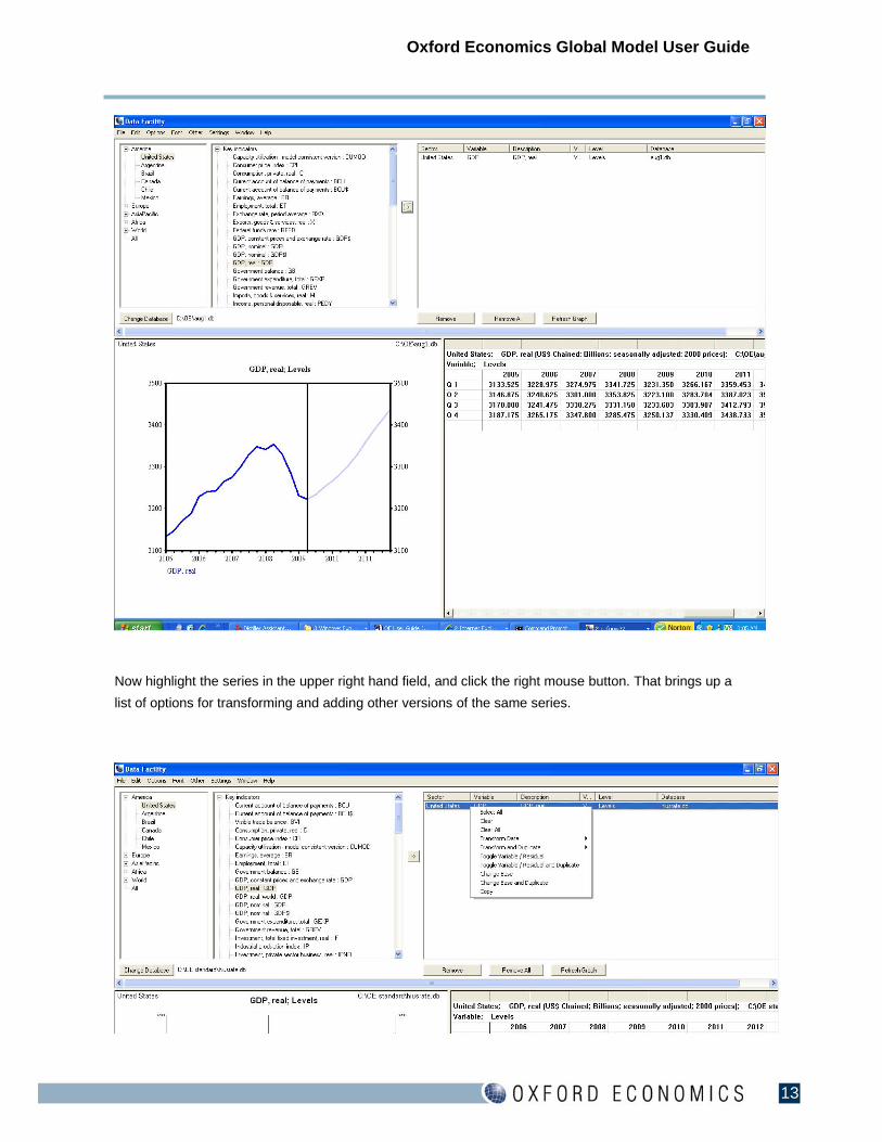
There is a wealth of information about the selected variable available to you on this screen. Each column

of data represents one calendar year – the four quarterly observations are listed above the annual total,

the average and the annual percentage change. Historical data, actual figures released by the

appropriate statistical agency, are displayed in black, while forecasts, supplied by Oxford Economics, are

in red. The left and right arrow keys can be used to shift the data table backward or forward in time.

Clicking on the button labelled var, res will replace the variable values with residuals. Over the historical

period, the residuals are the differences or the ratios (depending upon whether the equation was

estimated in level or in log form) between the equation calculation and the actual historical value. Over

the forecast period the residuals are set according to the forecasters’ judgment. By default the data are

displayed in their level form. However, several transformations are available. There is a list box to the

right of the variable name list box, which displays Levels when you start. Click on the down arrow to the

right to see the available transformations.


20

Click on another option, say Q-on-Q % Changes. This will alter the data displayed to the quarterly

percentage changes of the variable. To see a larger version of the graph, click on the graph icon in the

toolbar at the top of the page, just above the pulldown arrow for data transformations.

Again, colour is used to distinguish historical data from forecast data, with historical data in blue and

forecast in red. After clicking on the graph to activate it, the left and right arrow keys can be used to shift

the graph backward or forward in time, and the insert and delete keys can be used to add or delete years

of data.

Click on Info at the left end of the toolbar at the top of the screen and from the list choose Info on

current variable. The screen on the next page will appear.

In the upper left hand corner of the screen are repeated the database the variable has been drawn from,

the country the variable pertains to, and the series mnemonic. The data source is provided next. Then

the equation is provided. In some cases, as in the example above, the equation had been estimated in

log form: Ln(X) = c + aLn(y) + … . The equation is displayed in exponential form:

X = Exp(c + aLn(y) +... ), as it is incorporated in the model.

The equation is followed by is a listing of the variables that are directly affected by this variable – that is,

the equations for the variables on the list include some reference to the selected variable. In some cases,


21

where the equation is particularly long and/or there are many variables directly linked to the selected

variable, all of the information will not be visible on the screen. The scroll bar to the right will allow the

user to scan through all of the information. It is also possible to send this information to the printer. Just

select File and Print from the menu at the top of the screen.

Then there is the technical information. This includes the variable ID number, which is useful for some

special purposes, and just below are the variable and residual types. Variables may be endogenous,

exogenous or identities, and endogenous variables may have additive or multiplicative residuals. Finally

there is information on the date through which there is actual historical data, and a listing of

transformations that are in effect, if any.

Return to the variable data screen by clicking on the file icon to the left of the tool bar at the top of the

screen and selecting Close. Or you may instead choose to click on the X box at the right hand end of the

tool bar. Unless you have previously returned to the variable data screen, the graph of Q-on-Q

percentage changes will still be on the screen. If you need to, click on the graph icon to return to the

variable data screen.

4.2 Changing variable values

If the variable you wish to change is endogenous, that is, its forecast values are determined by an

equation, you have the option of changing the actual values or the residuals that are part of the

calculation of those values. If you change the values directly, you will have the further option of fixing the


22

values at your preferred levels or having the program calculate the residuals that on an ‘ex ante’ basis are

consistent with those values. Any means of changing variable values shown in the following sections will

work equally well on residuals. Similarly, any means of changing values will work whether the variable is

in level or transformed form.

4.2.1 Making changes directly

The simplest way to make changes is to the values of a variable is to type them directly onto the data

screen. This can be done whether the variable has been transformed or not. Still using German

consumption as an example, the data screen using the Q-on-Q percentage changes looks like this:

To enter a new value, double-click on the time period to be changed and enter the value desired. For

example, one could click on the percentage change shown for the fourth quarter of 2009, which has a

value of -0.20 in our example. Replace this with another value, say -2.0, and when you press the tab key

or enter key to accept the new value, the screen will look like this.


23

4.2.2 Making changes graphically

Variable values may also be changed graphically. To begin, click on Cancel to discard the changes

made so far and return the series to level form. Then click on the ‘graph’ icon to bring up the larger graph

of the series. Click on the graph, and a vertical arrow will appear on the line at the time period closest to

your mouse position.

+


24

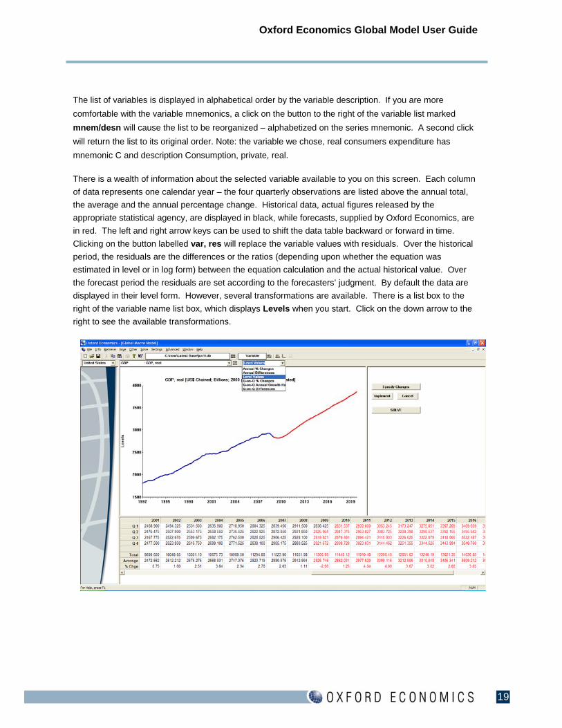
By holding the left mouse button down and moving the mouse up or down, you can pull the graph up or

down to the level desired. This process can be repeated for any period on the graph. To choose another

period to change, click near it or use the left or right arrow keys to move along the line to it.

For our example, we’ve inserted a spike in the series in 2010Q4. When you have made all the graphical

adjustments you wish, click on the ‘graph’ icon again so that the data display is again visible. Note that

the values for the periods you had pulled away from the original line have been changed, and so has the

chart.

The graph can also be used to interpolate between any two points. If you are following along with us,

click on the ‘graph’ icon and click on a point on the graph other than where you imposed the spike. Hold

down the control key while pressing the left or right arrow (toward the spike), and a line will be drawn that

interpolates between the first and last points. When you return to the variable data screen, you will see

that the values on the line have been transferred to the variable data screen. Note: If you hold down the

Alt key while pressing the left or right arrow keys, the graph will be held horizontal.


25

4.2.3 Specifying changes

The third way to make changes to variables is according to specified functions. To start, return to the

variable display screen and cancel any changes that have been made in this example. Click on the

button labeled Specify Changes in the body of the screen. This will bring up the dialog box:

There is a date range over which the change is to take affect. Note: this range will default to the full

forecast period, which may not match the period over which you wish the variable to be changed. Set the

range to the period you wish. Then, anything that is typed into the white box below will be applied over

that range. Say you enter the equals sign followed by the value 350. When you click on OK or press the

enter key, the screen will look like the one on the next page:


26

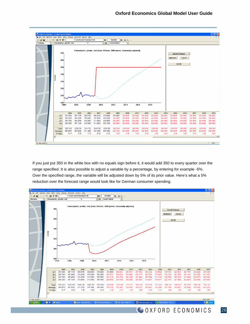
If you just put 350 in the white box with no equals sign before it, it would add 350 to every quarter over the

range specified. It is also possible to adjust a variable by a percentage, by entering for example -5%.

Over the specified range, the variable will be adjusted down by 5% of its prior value. Here’s what a 5%

reduction over the forecast range would look like for German consumer spending.


27

Finally, you can adjust a variable by means of an algebraic expression involving one or more other

variables. As a simple example, you might want to add a fraction of GDP to the level of consumption. To

do this you might enter .01*GDP. You can also make a variable a function of values in another country

(eg = .05*GDP, US to add 5% of each period’s value for US GDP).

4.2.4 Accepting changes

Once the user has made all changes desired to the selected variable, it is necessary to save the new path

by clicking on the button labeled Implement. If the variable is endogenous, the new values will be saved

and the variable will be fixed over the range affected by the change. If the variable is one of a set of key

identities, a message will appear to that effect, along with information as to which component variable or

variables will be adjusted to achieve the desired path for the identity variable. For example, if a change

had been made to German GDP, the following message would appear:


28

As mentioned, this is only the case for key identities in each country -- GDP or the unemployment rate, for

example. If you change other variables that are identities, such as nominal consumption (=real quantity x

price deflator/100) there will be no warning message and the identity will be broken. In general this

problem is easily avoided, since the model structure is consistent and (we believe) rational, and the

equations are well documented in the **EQNS.HLP files.

If the user has set values for a variable at a point in the future further than the first non-historical period, a

warning will appear: Imposing only these values will leave a gap in fixes for this variable - do you wish to

extend the fix back to the end of the last fix? In most cases the answer to this question is yes. Otherwise,

changes to other variables may cause movement in this variable in the unfixed periods, leading to an odd

jump in the series between the unfixed and fixed portions.

Once the variable change is implemented the user is free to select another variable to work on, which

might be from the same or a different country.

4.2.5 Ex ante changes

If the variable being adjusted is endogenous, the user has the option of adjusting forecast residuals rather

than the forecast values, as explained earlier. There is another option – the user can set a path for the

endogenous variable and have the software calculate the residuals that are consistent with that path on

an ex ante basis, that is, before equation interactions are considered. The equation remains active, and

will react to other changes during the simulation, so the final results will very likely differ to some degree

from the path set. To do this, simply click on the button labeled ex ante toward the right end of the

toolbar. Any endogenous variable changed while this option is selected will be made to the residuals

rather than the values.

Note: once selected the option will remain in effect until the user turns it off by clicking on the ex ante

button a second time. When the option is active, the button is a lighter grey than the surrounding toolbar.

4.2.6 Changing historical values

The sorts of changes we have been making to the forecast values of variables could also be made to the

historical values. This might be useful if data have been revised for the most recent time period and you

would like to see how this new information might affect the near term forecast. However, if you wanted to

try a more ambitious experiment, say altering fiscal or monetary policy several years ago to see the

outcome, simply changing the history and solving the model over the affected date range will not be

effective. This is because all of the other variables are fixed at their actual historical values, so the policy

change will have no effect. In this case, the user should first choose the Other option from the top

toolbar, followed by the option Add/Remove Fixes. The option Remove All Fixes should then be

checked, with the date range altered to reflect the historical period over which the counterfactual

simulation is to be run. This procedure ‘activates’ the model over the past, and counterfactuals can then

be conducted in the same way as simulations over the future, as described above.


29

4.3 Saving and retrieving run files

At times, it may be useful to save a runfile of changes that have not yet been incorporated into a data

base by solving the model. This might be the case if you’re making a lot of changes and need to stop

before all have been set. To save the runfile without solving, click on Save in the grey toolbar at the top of

the screen. This will bring up a dialog box that lists the runfiles currently available in the directory where

the OE software and databases are stored:

Provide a name for your runfile by typing in the box labeled File name. The filetype of .run will be added

automatically, and the run file of all of the changes that had been implemented during the session will be

saved to the OE directory.

To begin work with a previously created runfile, click on Retrieve in the grey toolbar at the top of the

screen. This will bring up a dialog box listing all of the available runfiles:

Click on the file you wish to start with. It will be read in, and any changes made subsequently will be

added to it.


30

5 Solving the Model Once you have implemented all the changes desired, click on the SOLVE button on the variable data

screen. The following screen will appear:

At the top of the screen are date ranges for the database solution period. Although the model solution is

very quick, you may want to abbreviate the solution period if you are only interested in a near-term

forecast. Solving the model over some of the recent past will not affect the solution.

The input database is the starting point for the solution. If you wish to start from a different database than

the default, click on the button to the left labeled Change. This will bring up a file opening screen which

will display all files with extension .DB in the folder where the OXFORD ECONOMICS software is stored.

Select one of them by clicking on it and then clicking on OK.


31

Similarly, you can change the output database by clicking on the Change button next to the default name.

The same file opening screen will appear. You can select a database that already exists – remember that

it will be overwritten by your new solution – or enter the name of a database to be created in the file name

field above the list of existing databases.

The Options button will bring up a dialog box that will allow you to control the solution in a number of

ways.

At the top are date range entries for the database storage period. Short-term baseline databases have

historical data beginning in 1980 and a forecast period of five years. However, the databases are fairly

sizable and the user may wish to crop them to save disk space. If you decide to shorten the storage

range, be sure that the range includes the year 1995, to supply data for lags used in the equations and to

facilitate data display and table generation. Once a database has been shortened, databases that are

created from it will also be short. It is not possible for the user to lengthen a database.

The box labeled Browse Run File Before Solving should be checked if you would like to scan the file of

changes that are being implemented. Don’t Solve – Just Create Base allows the user to add data or

equations to a database without solving the model, a feature that is useful when building a new model or

revising an existing one heavily, when it may be more convenient to have separate run files that must all

be implemented before attempting to solve the model. Don’t Recalculate WT/WP/WC base year values

should be checked if you’re doing a counterfactual historical simulation that starts before 2001. The

remaining boxes are for cycling through systems of models, a highly specialized application.


32

Click on OK to return to the screen where the input and output database names were set. The box in the

lower left labeled Include All Countries is checked by default. If you prefer to solve a subset of the

model, click on the box to clear it. When all selections have been made, click on OK.

If you have opted for a subset of the model, a country selection screen will appear. Choose the countries

to be solved by holding down the control key while selecting countries with clicks of the left mouse button.

The selected countries will be highlighted, as shown below.

Click on OK to continue. The model solution will begin. While the model solves a DOS box will pop up in

the applications bar at the bottom of the page. If you click on this box, it will open to show you the

number of iterations that the model takes for each time period as that period is solved.

When the solution is complete, you will be returned to the variable data screen. You will then be asked if

you wish to continue or update data files. Continue takes you back to the main menu screen. Update

Datafiles saves values for variables specified by the user to *.PRN or *.CSV files, which can then be read

into other packages (eg. spreadsheets). This is described further in Chapter 8.


33

6 Producing Tables

6.1 Oxford Economics supplied tables

To start, click on Generate Results Tables on the main options menu.That will bring up the following screen:

At the top of the screen is the name of a database, from which tables may be drawn. By default, this will

be the name of the last Oxford Economics baseline data installed or the last database created, but any

available database may be selected. To change the database names, click on the button labeled

Change to the left of the name. This will bring up a file opening screen which will display all files with

extension .DB in the folder where the Oxford Economics software is stored. Select one of them by

clicking on it and then clicking on OK.

Below is a space for a title that will appear on the standard tables. Then there is a date range for the

tables. It is often helpful to have a bit of historical data appear on the tables for comparison with the

forecast. Set the range by clicking on the appropriate box and replacing the years and quarters as

desired.

Just below, there is a toggle switch marked next to the text Standard Table List. In the large field

below are listed the standard table titles. The Standard Tables are a set of tables that display a variety of

series for one country at a time, providing an in-depth look at the forecast for any particular country or

countries.


34

Clicking on the toggle will replace the text beside it with Cross-Country Table List, and the titles of the

cross-country tables will be listed in the field as shown on the following page. The Cross- Country Tables,

which will contain only annual data, each display a particular variable for all countries, providing an easy

means of comparing the forecasts of more than one country.

The user selects whatever tables desired from either or both lists by clicking on the choices while

depressing the control key. The first selection offered on either list is all of the tables. Note: not all tables

are applicable to every country. For example, in the Standard Table List, after All Tables are 16 tables

common to all of the large country models, followed by names of several more tables that are specific to

one of three single countries, the UK, the US and China. In order to print Standard or Cross-Country

tables or both, it is necessary to click on the appropriate check box(es) to the right of the table list.

To the right of the date range is a pull down menu of possible kinds of percentage changes to be

calculated if quarterly tables are to be produced. The default is for annual percentage changes, which are

changes from the same period of the prior year, but you may prefer simple quarter-to-quarter percentage

changes or quarter-to-quarter changes expressed at an annual rate.

Below the check boxes for Standard and Cross-Country tables is another labeled Difference Tables. If

this box is checked, a table of the differences for key variables between two databases will be created.

Note: there is one standard difference table for each country. When you select difference tables, you will

be prompted with a standard windows file opening box for the name of the database to be compared

against. It is possible to create Difference tables at the same time that Standard and/or Cross-Country

tables are being created.


35

Choosing Options brings up the following screen.

The user may specify the Annual start Q, to switch between calendar years (start Q1) or fiscal years

(e.g. start Q2 in the UK). As you might expect, the box labeled Annual Data Only will limit Standard and

Difference tables to annual figures if checked. Finally, the tables format can be adjusted for reading

directly into spreadsheets. When your selection is complete, click on OK. If you have not chosen all

countries, the country selection screen will appear.

Select the countries desired by holding down the control key while selecting with the left mouse button.

Then click on OK. A window with the tables in it will appear, as shown on the following page. This is

actually a Windows browser, which will allow you to scroll through all of the tables created. The tables

have also been saved in an ASCII file, with the filename the same as the main database name and an

extension of .TAB, which can be printed later or pulled into other software, such as a word processor.


36

When you have finished viewing the tables, click on File and Exit from the toolbar or the X button in the

upper right hand corner to close the browser window.

6.2 User Tables

6.2.1 Setting up a table template

As well as printing standard tables provided by Oxford Economics, users can also print off tables

designed themselves. These tables are controlled by the information in template files, which the user can

set up to include specific table titles, subtitles, and data series and series descriptions to be included. To

create a template, choose Advanced Options in the main menu screen and then select Design User-

Tables from the new list.


37

The following screen will then appear. Clicking on the boxes labelled Title or Subtitle will bring up a dialog

box that requests the user to type in a text string that will appear in the table as a title (centered on the

page) or a subtitle (printed flush to the left). Clicking on Blank Line will insert a space into the table, while

Date Line will provide for dates to appear across the page.


38

Define Function is used if it is desirable to print data in a table that is not stored in the database but that

can be calculated from series that are in the database. The user types a mnemonic into the small box

and the calculation into the larger box, as shown below in the example to calculate nominal

consumption’s share of nominal GDP.

Clicking on Variable brings up the following dialog box, to collect information about the next line item to

be included in the table. Type the mnemonic in the first box. There are pull-down lists of countries and

mnemonics available to help the user find the mnemonics, but the information must still be typed into the

appropriate boxes. If the table is to include data from a single country, then the Sector/Country box may

be left blank (the country will be selected when the table is generated). If the table is to include data from

more than one country, then the Sector/Country box must be filled in. The variable mnemonic must be

either in the database or determined via the Define Function box.


39

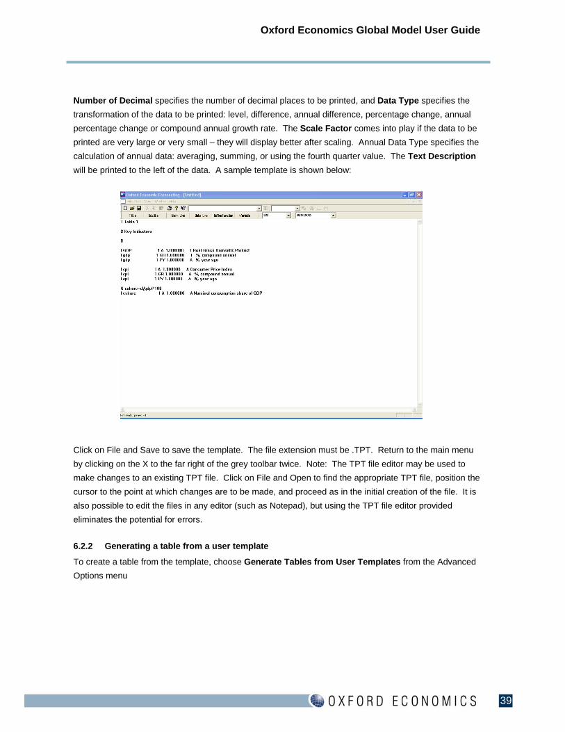
Number of Decimal specifies the number of decimal places to be printed, and Data Type specifies the

transformation of the data to be printed: level, difference, annual difference, percentage change, annual

percentage change or compound annual growth rate. The Scale Factor comes into play if the data to be

printed are very large or very small – they will display better after scaling. Annual Data Type specifies the

calculation of annual data: averaging, summing, or using the fourth quarter value. The Text Description

will be printed to the left of the data. A sample template is shown below:

Click on File and Save to save the template. The file extension must be .TPT. Return to the main menu

by clicking on the X to the far right of the grey toolbar twice. Note: The TPT file editor may be used to

make changes to an existing TPT file. Click on File and Open to find the appropriate TPT file, position the

cursor to the point at which changes are to be made, and proceed as in the initial creation of the file. It is

also possible to edit the files in any editor (such as Notepad), but using the TPT file editor provided

eliminates the potential for errors.

6.2.2 Generating a table from a user template

To create a table from the template, choose Generate Tables from User Templates from the Advanced

Options menu


40

The database from which the table is to be created is chosen as well as a name for the ascii file that will

save the table. The default for the table file is TPTABLES.TAB. Click on change to choose an alternative

filename.

The box on the left headed Standard Templates gives a selection of pre-formatted tables which appear in

Oxford Economics documents. The box Other Templates on the right-hand side allows the user to

update a template table of his own design. Clicking on Other Templates gives a menu of all the .TPT files

available in the user’s working directory, from which the required table can be selected.

Quarterly, annual and 5-year average data are selected by checking the boxes in the middle of the

screen, while the user can choose the date range in the boxes alongside. Options allows users to alter

the start quarter for actual calculations (e.g. calendar vs. fiscal years) and to calculate differences or

percentage differences between two databases. In addition, the table output can be controlled by altering

the number of significant digits to be printed, the line length and the number of lines per page. If both

annual and quarterly date ranges have been set, the user can choose to have the annual data appear to

the left of the quarterly data (the default is for the quarterly data to appear first). Finally, the user can

choose "Comma/Quote Delimited Output" for easier importing of the resulting file into a spreadsheet.

Having selected the user-defined tables to be updated click OK and specify the countries required as with

Oxford Economics supplied tables. The resulting table will be displayed in the Windows browser, as

described in the previous section. The tables can be sent to a printer or pulled into other software, such

as a word processor.


41

The template shown as an example on the previous page was saved to a file called TEST.TPT. In the

example above, this template was chosen from the Other Templates selection, quarterly data for 2009

and annual data for 2008-2010 were selected. On the country selection screen, the US and Germany

were selected. The resulting table is shown below.

Note: The Standard Templates include templates for the Cross-Country tables described in the previous

section. They are labelled OV1.TPT, OV2.TPT, etc. These templates can be used, as shown in the

example below, to produce those Cross-Country tables on a quarterly basis. If you wish to create these

Cross-Country tables in this way, do not select All Countries, even though data from all countries will be

included. Rather, on the country selection screen, click on a single representative country to generate

one copy of the table(s) selected. If you select All Countries, you will generate one copy of the selected

tables for each of the individual countries in the model. While this will do no harm, the listing generated

will be quite long and the process could take quite some time.


42


43

7 Pre-Defined Scenarios There are some pre defined scenarios in the model where changes to the model have been already made

and will run automatically once selected. For example a shock such as an increase in the world oil price

can be applied to the model before tables are used to examine the impact of the shock on different

countries and different variables. Click into the Pre-defined Scenarios option on the main menu and the

screen below will appear.

There currently are 5 pre-defined scenarios-

1. The world oil price variable WPO is raised by $10/barrel from 2010 Q1 to 2018 Q4.

2. A 10% US dollar devaluation is imposed from 2010 Q1 to 2018 Q4.

3. A 20% revaluation to the Chinese yuan against the US$, which assumes that all other Asian

currencies follow suit. This is imposed from 2010 Q1 to 2018 Q4.

4. A 50 basis points increase in the US federal funds rate from 2010 Q1 to 2010 Q4.

5. A 50 basis points increase in the ECB Interest Rate from 2010 Q1 to 2010 Q4.

To run the oil shock, click on the option $10/barrel increase in the world oil price. Choose a name for

the output file and save it and click ok. The screen on the next page will pop up. If you wish to look at

results for all countries, tick the box at the top which says all countries. Otherwise select the countries you

wish to include individually.


44

A CSV workbook will be created automatically and will show standard Oxford Economics created tables,

as discussed in chapter 6. For each country selected there will be two tables of summary items. After all

the summary items tables there will be a list of difference tables, one for each country and showing the

differences to key variables in the model from before and after the oil price shock.


45

8 View and Download Data This section provides a means of collecting data of interest from one or more databases, displaying it in

either level or transformed form and downloading it to files that are accessible by other software

packages. To start, click on View and Download data from the main menu. That will bring up this screen:

8.1 Displaying data

The screen is divided into four roughly equal sections. In the upper left corner are two boxes. The

leftmost contains a list of regions and the one to the right a list of economic sectors. Beside each entry in

these lists is a small box containing a plus sign. Clicking on the plus sign will open up sublists for each

region and sector, as shown below.


46

Where the lists have been expanded, the plus sign has been replaced with a minus sign. Clicking on the

minus sign next to a region or sector name will collapse that particular list again. You may select one or

more countries from one or more regions by clicking on them while holding down the control key. Then

you would select one or more variables from one or more sectors in the same manner. When the series

have all been identified, click on the right arrow button in the middle of the top half of the screen. We

chose real GDP from the US and Canada.

Now there is information in the other three sectors of the screen. In the top right block, there is information

on the variables that were selected, including the country, the variable mnemonics, the variable

descriptions, the transformation if any, and the database from which the variables were drawn. In the

bottom left block is a chart of the variables, with the historical data distinguished from forecast both by

means of a vertical line and the intensity of the lines. The magnitude of the two variables are very

different, with the levels of Canadian data much larger than US GDP because GDP is reported in millions

in Canada but billions in the US. Click on the F5 function key to cause the graph to switch to different

scales on the two vertical axes. In the lower right hand block the data themselves are displayed, in

spreadsheet form. The scroll bar beneeth the data listing can be used to display earlier data or data

further into the forecast period.


47

You can change the periods displayed in the chart by clicking on it and using the insert and delete keys to

lengthen or shorten the periods shown, while the left and right arrows can be used to move the display

back through history or forward to the end of the forecast period. Similarly, you can move the data display

in the lower right block forward and back through time by means of the scroll bar beneath it.

8.2 Defining functions – to be added

8.3 Transforming data

Our example in Section 8.1 displayed the data in level form. However, it is possible to transform the data

in a number of ways, and to bring in the same series from a different database without returning to the

data lists. To do this, in the upper right-hand box, highlight the series to be transformed or to be pulled

from another base. Right click on the one of the highlighted series, and a box of options will appear:

The first few options will allow you to select all the series on the list or clear all or selected series from the

list. The fourth is to transform data series, which will replace the series highlighted with the desired

transformation of the same series, while the fourth, to transform and duplicate leaves the original series in

place but adds the transformed series to the list. In the example above, we’ve opted to transform the data

as additional series. The transformations available are: Annual Percentage Changes and Annual

Differences (both of which produce series of quarterly changes calculated against the same period of the

previous year), Levels, Q-on-Q Percentage Changes, Q-on-Q Annualized Growth Rates and Q-on-Q

Differences (the Q-on-Q transformations also provide quarterly values, but the calculations are against

the previous quarter) and then a number of ways of calculating annual values: as Annual Totals, Annual

Averages, Last Quarter, Percentage Changes between 4th quarters, and Percentage Changes of Annual

Values.

Going back to our example, we chose Annual % Chges, which added two items to our list of series, the

percentages changes calculated against the year-earlier quarter in US and Canadian GDP. The data

have appeared automatically in the spreadsheet corner of the page, but the graph will not change until


48

you highlight the new series and click the Refresh Graph button at the bottom of the series list box. The

screen then appears like the one below.

In addition to transforming series, there are options to show the equation residuals for the selected

variables, again either replacing the series data or adding additional items to the list. Most users are

more likely to want to pull in data from a different database. As shown in the screenshot on the previous

page, these options are also provided. With the annual percentage change variables still highlighted, we

right-click on one of them and selected Change Base and Duplicate. This brought up a list of available

databases. We selected on, an oil shock scenario, and two new lines were added to our list, for the

annual percentage changes in GDP for the US and Canada but drawn from the second base. The data

appear automatically in the spreadsheet part of the screen, but the chart won’t change until Refresh

Graph button is pushed. We selected the percentage changes for the US and Canada (by selecting while

holding down the control key) and refreshed the graph. The resulting screen is shown on the following

page.


49

8.4 Exporting data

There are a couple of different ways to save data to another type of file. The simplest way is to copy and

paste. Once you have data in the spreadsheet grid in the lower right hand side of the screen, highlight the

data that you want to save, and then click the right mouse button. That will bring up a box of three

options: Copy, Select All, and Change Display Dates. Choose Copy, then move to an excel sheet or a

notepad session or other program environment. Then right click on a file open in that environment, and

choose paste. The data will be transferred to the excel sheet or other file, exactly as it appears on the

View and Download Data screen. Note: if you start to highlight the series from the far left column of period

labels, the data will be saved from the start of the database, 1980 in most cases.


50

Another way to save or export data is to highlight the desired series, then click on Save or Save As from

the File menu. That will bring up the following dialog box:

Checking the fourth box, labelled Save all information and data to PRN file, and then clicking on OK

will create an ascii file in column format, as shown below.


51

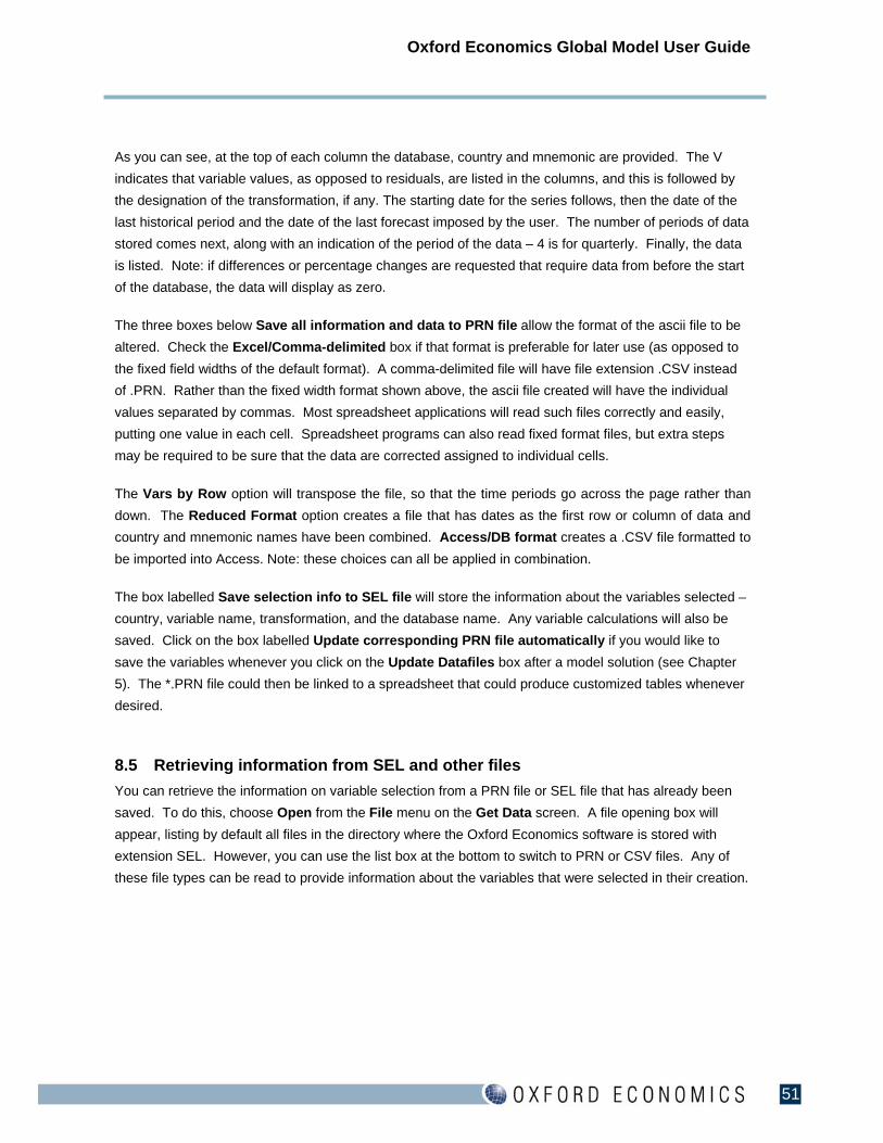
As you can see, at the top of each column the database, country and mnemonic are provided. The V

indicates that variable values, as opposed to residuals, are listed in the columns, and this is followed by

the designation of the transformation, if any. The starting date for the series follows, then the date of the

last historical period and the date of the last forecast imposed by the user. The number of periods of data

stored comes next, along with an indication of the period of the data – 4 is for quarterly. Finally, the data

is listed. Note: if differences or percentage changes are requested that require data from before the start

of the database, the data will display as zero.

The three boxes below Save all information and data to PRN file allow the format of the ascii file to be

altered. Check the Excel/Comma-delimited box if that format is preferable for later use (as opposed to

the fixed field widths of the default format). A comma-delimited file will have file extension .CSV instead

of .PRN. Rather than the fixed width format shown above, the ascii file created will have the individual

values separated by commas. Most spreadsheet applications will read such files correctly and easily,

putting one value in each cell. Spreadsheet programs can also read fixed format files, but extra steps

may be required to be sure that the data are corrected assigned to individual cells.

The Vars by Row option will transpose the file, so that the time periods go across the page rather than

down. The Reduced Format option creates a file that has dates as the first row or column of data and

country and mnemonic names have been combined. Access/DB format creates a .CSV file formatted to

be imported into Access. Note: these choices can all be applied in combination.

The box labelled Save selection info to SEL file will store the information about the variables selected –

country, variable name, transformation, and the database name. Any variable calculations will also be

saved. Click on the box labelled Update corresponding PRN file automatically if you would like to

save the variables whenever you click on the Update Datafiles box after a model solution (see Chapter

5). The *.PRN file could then be linked to a spreadsheet that could produce customized tables whenever

desired.

8.5 Retrieving information from SEL and other files

You can retrieve the information on variable selection from a PRN file or SEL file that has already been

saved. To do this, choose Open from the File menu on the Get Data screen. A file opening box will

appear, listing by default all files in the directory where the Oxford Economics software is stored with

extension SEL. However, you can use the list box at the bottom to switch to PRN or CSV files. Any of

these file types can be read to provide information about the variables that were selected in their creation.


52

Once you have retrieved the variable list, you can edit it, adding or deleting lines. If the variables in the

reopened SEL file are from more than one database, then the file will be opened exactly as it was

created. However, as a special case, if all of the variables were chosen from the same database, the

following dialog box will appear:

If you click on Yes, then the database name in the SEL file, NOV1.DB in this case, will be replaced with

the name of the currently opened database. This will allow the user to update the series in a PRN or CSV

file whenever desirable.

8.6 Settings

There are a number of settings that may be adjusted in View and Download Data according to the user’s

preferences. They are found by clicking on Settings in the grey toolbar at the top of the page.


53

The first option Number Format will bring up a dialog box to check whether very large and very small

numbers should be expressed in scientific notation. The default sets scientific notation on.

The second option is to switch the display of the series within each sector between alphabetized by

description (the default) and alphabetized by mnemonic. Once set, each of these first two option will

remain in force until the user explicitly changes them, even if the software is closed down and reopened.

The remaining options are only set for a specific session. They are used to restrict the lists in meaningful

ways. One is to list only those variables that appear in common among the countries specified and

another is to list only those variables that exist in at least one of the countries specified. For example, if

we select the US and Canada, and then expand the list for GDP and Domestic Demand, the list of

variables includes such variables as Consumer expenditure, rural and Consumer expenditure, urban. But

those concepts don’t exist for either the US or Canada (they can be found in the China model). If we

select either of the two restrictive settings, the Chinese variables will disappear from the list.

Finally, the setting to list all variables returns the lists to the default condition. And as mentioned, the

restrictive settings will have to be reset if desired in a subsequent session. This is because there is a cost

in terms of the time required to create the customized lists any time the user changes the countries

selected.


54

9 The Alternative Data Facility In addition to the data facility described in the previous section, we have retained an earlier version.

We’ve done this because the data are organized in a different fashion, which may be easier for some

purposes.

As in the case of the main data facility, the alternative data facility is used to gather data from databases.

Selected data series can then be graphed, listed or exported to various types of files that are compatible

with other software packages. The data may be in level form, or they may be transformed in one of

several ways. In addition, it is possible to calculate expressions involving one or more variables from a

database. To begin, click on the Advanced Options icon on the main menu and then click on the

Alternative Data Facility option.

9.1 Selecting variables

The toolbar at the top of the screen contains a list box for the database name. To switch to a different

database, click on the chge base button to the right of the list box, locate and highlight the name of the

desired base on the list, and click on OK to make the selection. There is another list box on the toolbar

that allows the user to toggle between actual values and residuals for endogenous variables. Most of the

time, this will be left set to Variable.

Below the toolbar are three additional list boxes, for the selection of the country, variable, and

transformation. To change the selections, click on the arrow to the right of each list box, then locate and


55

highlight you selection. Note: the first six choices in the transformation list box provide quarterly data, in

level, q-on-q % changes, compound growth rates, or differences, and annual % changes and differences

calculated from the same period of the previous year. The final four options are for annual data. For

annual % changes, the annual values are calculated first, then the % changes.

When the list boxes identify the desired variable, click on the button labeled Add to End. This will put a

line identifying the selection into the large box to the left of the screen. Continue using the list boxes to

identify other series and add those lines to the end of the list. If you want to place a series in the middle

of the list rather than at the end, highlight the line you would like it to precede and click on Insert instead

of Add to End. To remove a line from the list, highlight it and click on Remove. Your screen will look

something like this:


56

If you would like to reorganize the screen so that variables are grouped more logically, click on Sort. This

will bring up a box of options for sorting the series. Select one or more of the criteria offered to reorganize

the list.

The button labelled Get Function allows the user to specify an expression to be used to calculate a new

variable not in the database from a variable or variables that are in the database. For example, the user

might wish to calculate the ratio of exports to GDP. After clicking on the Get Function button, this box

will appear:

Type a mnemonic of your choosing into the first box, and if you wish, a description of the variable into the

second. Type in the expression to be calculated in the third box. The example here shows the calculation

for the export share of GDP. When you click on OK, the series will be calculated, using data from the

country that is currently selected. A line referring to the mnemonic you have selected will be entered into

the box of selected variables. The calculated data may then be displayed, graphed, or saved to an ascii

file, just as any series from the database.


57

Note: the series calculated is a temporary variable. It is not stored on the database. To add series and

equations to the database, see Chapter 11. However, the calculation will be retained during the session,

so that if you want the same transformation calculated for several countries, you would create it for the

first country, as described above, then switch to the second country, click on Get Function, and type in the

name of the mnemonic you had chosen for the first country. When you click on the description or function

area or on OK, the entries from the first country will be recalled, and entries added to the variable

selection box, as shown below. Note: there is no case distinction.

9.2 Displaying data

Any series listed in the box of variables, whether in level form or transformed and whether a series from

the database or one that was calculated via the Get Function screen, may be displayed. Highlight the

selected series by clicking on it – only one series may be selected to be displayed at a time – and click on

the button labelled Display Data. The data will be shown in the same Windows browser that is used to

display tables. The data are arranged by year, as shown:


58

9.3 Graphing variables

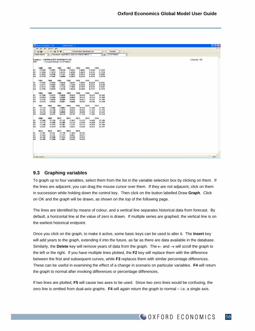
To graph up to four variables, select them from the list in the variable selection box by clicking on them. If

the lines are adjacent, you can drag the mouse cursor over them. If they are not adjacent, click on them

in succession while holding down the control key. Then click on the button labelled Draw Graph. Click

on OK and the graph will be drawn, as shown on the top of the following page.

The lines are identified by means of colour, and a vertical line separates historical data from forecast. By

default, a horizontal line at the value of zero is drawn. If multiple series are graphed, the vertical line is on

the earliest historical endpoint.

Once you click on the graph, to make it active, some basic keys can be used to alter it. The Insert key

will add years to the graph, extending it into the future, as far as there are data available in the database.

Similarly, the Delete key will remove years of data from the graph. The and will scroll the graph to

the left or the right. If you have multiple lines plotted, the F2 key will replace them with the difference

between the first and subsequent curves, while F3 replaces them with similar percentage differences.

These can be useful in examining the effect of a change in scenario on particular variables. F4 will return

the graph to normal after invoking differences or percentage differences.

If two lines are plotted, F5 will cause two axes to be used. Since two zero lines would be confusing, the

zero line is omitted from dual-axis graphs. F4 will again return the graph to normal – i.e. a single axis.


59

The TITLE can be replaced by clicking on it and editing it as desired, and it can be centered between the

axes by clicking on the far right icon in the toolbar at the top of the screen. The colour-coded labels at the

bottom of the page may also be edited, and they can be repositioned on the graph by clicking on them

with the right mouse button and dragging them to the desired location. When the right mouse button is

released, the label will be dropped into place. Double-clicking with the left mouse button will cause the

word Text to appear at the cursor position. This text can be edited and repositioned to enhance the

graph.

By default, the variables are displayed as lines, on the same scale, which is shown on both sides of the

graph. To adjust these and other parameters, click on Options in the toolbar at the top of the screen,

which will bring up the screen shown at the top of the next page.

The first four check boxes control whether the horizontal zero marker and the vertical forecast line are

present, whether the Y-axis is labeled on both sides of the graph (for single axis graphs only) and whether

the quarterly tick marks are shown on the X-axis. The frame width refers to the thickness of the lines

used in the graph box, the zero marker and the forecast line. The < and > buttons can be used to alter

this thickness.

The rest of the options pertain to the lines of the graph. Set the options for each line in turn. Line 1

comes up by default, and you can see its label in the box to the right. Just below you will see the

thickness of the curve, which can be adjusted as described above for the frame width. All of the option


60

choices will be retained by the software to be used for subsequent graphs. At the bottom of the screen

are list boxes to change the colour of the line and the line style (solid, dash or dotted). To the right, the

minimum and maximum scale values are displayed. If you wish, you can alter the scale by clicking on the

values and overtyping, but you must also click on the override checkbox above for the new scale to be

implemented. Finally, there is an option to switch the variable from a line to a bar plot.

We have found it useful to keep two sets of options, depending on whether the graph is to be printed on

paper or made into an overhead transparency. The button labelled Output will switch between the two

sets of parameters.

To use the final graph in another application, such as a word processor, click on Edit, Copy from the

toolbar, or the copy icon. You will be asked to select the type of output to be created – that is, which set

of option parameters to use, for solid (Normal) or transparency. For a word processor, select solid.

Switch to your word processor application. The remainder of this instruction is for Word – details may

differ for other word processors. Click on Edit and Paste Special and Picture. The graph will be placed in

your document, but it will be tiny. Click on it, and you will see the resizing points appear. Click on the

lower right hand corner and drag, and the graph will be expanded. That is how the graph just below was

pulled into this document. (Other graphs shown in this document were imported as screen captures.)


61

It is also possible to print the graph from within the Oxford Economics software. To send the graph to the

printer, click anywhere on the graph to make it the focus. Then either click on the printer icon in the

toolbar or select Print from the File menu. You may first want to select Print Setup from the File menu to

set such options as the paper size and orientation. If the printer is a colour printer, the graph will be

displayed as shown on the monitor. With a black and white printer, the graph will identify lines by line

style – solid, dotted and so on. There will be no distinction between historical and forecast data.

9.4 Saving data

To save the data for the variables you have selected, click on Save or Save As from the File menu.

2006 2007 2008 2009 2010 2011 2012-6

-4

-2

0

2

4

6

-6

-4

-2

0

2

4

6

GDP; Annual % Changes;

GDP / United StatesGDP / Germany


62

Checking the fourth box, labelled Save all information and data to PRN file, and then clicking on OK

will create an ascii file in column format, as shown below.

As you can see, at the top of each column the database, country and mnemonic are provided. The V

indicates that variable values, as opposed to residuals, are listed in the columns, and this is followed by

the designation of the transformation, if any. The starting date for the series follows, then the date of the

last historical period and the date of the last forecast imposed by the user. The number of periods of data

stored comes next, along with an indication of the period of the data – 4 is for quarterly. Finally, the data

is listed. Note: if differences or percentage changes are requested that require data from before the start

of the database, the data will display as zero.

The three boxes below Save all information and data to PRN file allow the format of the ascii file to be

altered. Check the Excel/Comma-delimited box if that format is preferable for later use (as opposed to

the fixed field widths of the default format). A comma-delimited file will have file extension .CSV instead

of .PRN. Rather than the fixed width format shown above, the ascii file created will have the individual

values separated by commas. Most spreadsheet applications will read such files correctly and easily,

putting one value in each cell. Spreadsheet programs can also read fixed format files, but extra steps

may be required to be sure that the data are corrected assigned to individual cells.

The Vars by Row option will transpose the file, so that the time periods go across the page rather than

down. The Reduced Format option creates a file that has dates as the first row or column of data and

country and mnemonic names have been combined. Access/DB format creates a .CSV file formatted to


63

be imported into Access. Note: these choices can all be applied in combination.

The box labelled Save selection info to SEL file will store the information about the variables selected –

country, variable name, transformation, and the database name. Any variable calculations will also be

saved. Click on the box labelled Update corresponding PRN file automatically if you would like to

save the variables whenever you click on the Update Datafiles box after a model solution (see Chapter

5). The *.PRN file could then be linked to a spreadsheet that could produce customized tables whenever

desired.

9.5 Retrieving a .PRN, .CSV or .SEL file

You can retrieve the information on variable selection from a PRN file or SEL file that has already been

saved. To do this, choose Open from the File menu on the Get Data screen. A file opening box will

appear, listing by default all files in the directory where the Oxford Economics software is stored with

extension SEL. However, you can use the list box in the lower left corner to switch to PRN or CSV files.

Any of these file types can be read to provide information about the variables that were selected in their

creation.

Once you have retrieved the variable list, you can edit it, adding or deleting lines. If the variables in the

reopened SEL file are from more than one database, then the file will be opened exactly as it was

created. However, as a special case, if all of the variables were chosen from the same database, the

following dialog box will appear:


64

If you click on Yes, then the database name in the SEL file, NOV1.DB in this case, will be replaced with

the name of the currently opened database. This will allow the user to update the series in a PRN file

whenever desirable.


65

10 List information from Database There are several ways of listing information from a database in quantity that may be useful to the

forecaster. To begin, click on Advanced Options on the main menu. Then select List Information from

Database. The following screen will appear:

At the top of the screen is the default database. If you wish to create listings from a base other than the

one listed as the main base, click on the Change button to the left. A standard Windows file opening box

will appear. Select the base you prefer, and click on OK.

Enter a title if you wish. This title will appear at the top of the listing created. Set the date range by

clicking on the appropriate boxes and resetting the values. The date range is applicable to the Variables

and Residuals, Differences, and Percentage Differences listings.

If you check the box beside Variables and Residuals, you will create an ascii file that contains for each

variable in each country selected, and for each time period in the date range, the equation calculation, the

residual, and the variable value. A portion of such a file is shown below. For the periods over which the

variable is fixed, the third column, labelled Act/Fcst, contains the actual historical data, and the value in

the Residual column is calculated as the actual less or divided by the computed value (depending on

whether the residual is additive or multiplicative). Over the forecast period, the Act/Fcst column contains

the forecast values, and has been calculated as the computed value plus or times the residual, which has

been set by the forecaster. Note: if the box marked All Countries is checked, the listing generated will

be very large.


66

The box labelled Fixes and Equations provides two types of information in one ascii file. First, the

equations for all of the endogenous and identity variables in the countries selected are listed. However,

the equations are written using variable locations, with series mnemonics listed below. The same

information is provided in a far more readable form in the equation help files, and if you would like a

complete listing of any countries’ equations, we recommend browsing or printing these files.

The second type of information is a summary of the fixes that apply on all of the data for the selected

countries. The last historical data period can be identified by the type 1 or (rarely) a type 2 fix on the data

point. If the database is one that you have created by altering assumptions and solving the model, there

will be type 3 and type 4 fixes as well indicating variable values have been imposed for the future. Note: if

the box marked All Countries is checked, the listing created will, again, be very long.

The boxes labelled Differences and Percentage Differences provide a means of comparing every

variable in a database with its counterpart in another database. If you have made a model solution, the

starting base will be the default for the comparison database. Otherwise, the Base for Diffs will be empty

and you will be prompted for the name of the base to compare against. To the right are threshold values,

below which differences or percentage changes are considered to be insignificant. The actual or

percentage differences are calculated over the range specified, and then listed in a fairly concise

columnar form, as shown below. Periods for which no variables show changes above the threshold are

not shown, as are any variables that have no change above the threshold over their entire range.


67

Finally, if the box labelled Coefficients is checked, a listing of coefficients will be generated. Country

selection has no impact on this listing. The coefficients listed are not the coefficients of the model

equations. Rather they are values that control the simulation – determining the number of iterations

allowed per period, setting convergence criteria, determining which of the country models will be solved,

etc. The listing provides no information as to the role of each coefficient, so we recommend viewing, and

changing these coefficients if you wish, through the Other option, which is described in Chapter 11.


68

11 Advanced Facilities There are several additional capabilities that are available. These functions are accessed from the

Variable Data screen, which appears when the Run Model button is selected from the main menu. In the

toolbar at the top of the screen, the third option is Other. Click on this option, which will produce a pull-

down menu.

11.1 Add/Update Equations

The first option is to supply new equations to the model. These may be replacements for existing

equations or equations for variables that are new to the model. Click on Add/Update Equations:


69

The three buttons for the top are to be used if there are equations stored in a file. If the equations were

estimated in TSP or PCGive, click on the appropriate button and, when the file opening box appears,

select the file of equations to be opened. The equations will be read and, assuming no errors are found,

a message will appear to indicate that the equations have been processed.

If the equations were estimated in some other statistical package or are from some other source, then it is

still possible to read them into the model by clicking on the first button, labelled Eqns from EQN file and

then selecting the file. It is important that the file of equations follows some conventions:

The equations are to consist of algebraic combinations using standard operators and the variable

mnemonics. (Four digit variable identifiers are also permissible, but mnemonics are more convenient.)

The equations must be in simple form. That is, the left hand side of each equation must consist of one

variable, which may be transformed into log form or change form. It cannot be, say, the ratio of two

variables.

Operators are:

+ - * / ( )

** Exponentiation

Reserved words (do not use as mnemonics)

Tyyp Time trend set to 1 in year yy period p and incremented by 1 each period

If yyp is omitted, it is assumed to be 701.

Qn Period switch, set to 1 if current period is n, else 0.

Functions (do not use as mnemonics) Note: all arguments are to be in parentheses.

exp Exponential

ln Natural logarithm

log Natural logarithm

abs Absolute value

dn Difference between current period and n periods back. If n is omitted, it is

assumed to be 1

sn Sum between current period and n periods back. If n is omitted, it is

assumed to be 1

R Residual


70

Blank lines in the equation file will be ignored. A % in the first column of a line indicates that the line is a

comment, which can be very useful for documenting the equations. The % is also used as a continuation

character – if the equation will take more than one line (80 characters per line), the first line(s) should end

with the %. The maximum number of characters in an equation is 1000.

The equations will be checked for syntax and variables. A message will be displayed when any syntax

problem is encountered, but processing will be allowed to continue so that any other errors can be

spotted. If an equation defines a variable for which data have not been provided, the variable will be

added to the model with zero values. Any right hand side variable that is not already in the database or

defined by one of the equations in the EQN file will be flagged. It can be added to the model as an

exogenous variable and data can be added before the model is run.

Note: the equation help files provided for each country in the model are valid EQN files.

The equation active dates and the equation type options do not apply to equations entered from a file.

By default, equations entered are assumed to be behavioral, that is they are endogenous with residual

terms. The residuals will be additive in the equation is stated in level terms, but multiplicative if the

equation is stated in log form (this may be overridden by explicitly including a residual term in the

equation). Also by default, the equations entered will be active over the entire range of the database.

They are made active over the historical part of the database so that historical residuals can be

calculated. These are useful both in checking the accuracy of the equation and as a guide to setting

residuals in the forecast period.

However, if you wish to restrict the range of your equations, you may do so by preceding them in the in

the EQN file with a line containing the letter Q and the date range in the following format:

Q YYYY P YYYY P

The range will apply to all subsequent equations until a new range is encountered.

Similarly if you wish to force an equation to be an identity, it should be preceded by a line that starts with

an I. The I may be followed by a date range as above if desired. Only the equation directly following the I

line will be affected.

It is also possible to force a variable to be a transformation, which means that instead of being solved

during each iteration, it is calculated only once for each time period before the iterations begin. This type

of equation is used by OXFORD ECONOMICS forecasters in some cases to calculate historical values

that are determined by other variables in the database or to manage the forecast of residuals or

exogenous variables. This is done by replacing the Q or I with a T in the line before the equation.

However, it is not recommended in general for client use.

Note: The equations in the file will be added to the model for whatever country is active on the Variable

Data screen. If you want to apply the same set of equations to more than one country, you will add them

to the first country, then return to the variable data screen to reset the active country, then go back to

Add/Update equations, and so on.


71

If you are adding just one or two simple equations and do not wish to keep them in a file, then you may

enter them directly. For example, if you wanted the exports share of GDP to be a model identity, you

would enter the calculation in the box, as shown below:

Identifying the variable as an identity will prevent a residual term from being added. Checking on the

Transformation box will cause the equation to be calculated just once per time period, as described.

However the equations are entered, they are converted to lines in a run file. The variable mnemonics are

replaced with six-digit variable identifiers, and if the equation is in log form, it is translated to level form.

The equations will not actually be added to the database until the model has been solved with that run

file. It is a good idea when solving the model to add equations to solve it over at least some portion of

history so that the historical residuals will be calculated. Note: do not solve the model from the beginning

of the database – without necessary lags it will fail. Allow at least 2 years from the beginning of the

database before you solution period.

Note: Equations added to the model are permanent in the sense that they will be included in any

databases created from the database to which the equations were added. Thus, you can add or change

equations and then run model shocks to check on the equations’ properties without adding the equations

for each run. However, the new equations will of course not be in the next release you receive from

Oxford Economics, so if you wish to keep them, they will have to be added again. Thus, it will be very

important to keep the file of equations, or if you entered the equations directly, the run file.


72

11.2 Add/Update Variables

When updating values for a large number of series, for example, when new national accounts data are

released, it is possible but cumbersome to use the variable change screen for each in turn. However,

there are several formats that can be used to update quantities of data quickly. It takes a bit of time to set

up initially, but worth the effort if the data set will be updated frequently.

After clicking on Add/Update Variables, a Windows file opening screen will appear. In the lower left

corner, a pulldown menu lists possible file types. The most common type of file to use, and the one used

for most of our own updating, is a spreadsheet file. Click on Spreadsheet (*.WK3) or on Spreadsheet

(*.XLS) and then on the file holding updates, and the following screen will appear:

The options allow for complete or partial updates from the spreadsheet. Select an option, click on OK,

and the data will be processed into a run file. For the data to be incorporated into a database, the model

must then be solved, starting in the earliest period for which data is provided.

Getting the data into a valid WK3 or XLS file is up to the user. Here is a portion of a valid WK3 file. The

structure of the file must follow the example exactly, but in general, there is no distinction between upper

and lower case, and column widths and fonts may be set as desired.


73

The label ‘OEF mnemonic’ must be found in a cell in the spreadsheet. All of the rest of the information is

found relative to this base cell. The time series are defined in columns to the right of the base cell. There

may be blank columns, but all data in the sheet must conform to the required format. NA values are

acceptable. The series mnemonics are defined on the same row as the base cell; they are labels of a

maximum length of fifteen characters and may be justified as the user desires for ease of reading.

The country definition (maximum eight characters) is on the next row. Any one spreadsheet can hold

data for one or more countries or regions. It is formated as a label. If you are updating an OXFORD

ECONOMICS World Macro database rather than a database of a model you have built yourself (which

would have country/region names as you defined them), the country/regions must come from the

following (current) list (note, long country names must be clipped exactly as shown here):

US CZECH ROMANIA

JAPAN DENMARK RUSSIA

EURO_11 FINLAND SINGPORE

GERMANY GREECE SLOVAKIA

FRANCE HK SAFRICA

ITALY HUNGARY SPAIN

UK INDIA SWEDEN

ARGENTIN INDONESI SWITZ

AUSTRALI IRELAND TAIWAN

AUSTRIA KOREA THAILAND

BELGIUM MALAYSIA TURKEY

BRAZIL MEXICO RESTOECD

BULGARIA NETH OPEC

CANADA NORWAY EASTEUR

CHILE PHILIPPI AFRICA

CHINA POLAND LATAMER

CROATIA PORTUGAL RESTWORL WORLD


74

The Variable/Residual row must contain either the label ‘VAR’ or ‘RES’ for each data column. Normally

only variables would be present, but the ability to read in residuals is also provided.

The rows labeled ‘Dataset source’, ‘Data of data (YYMMDD)’, and ‘Source Mnemonic/Transformation’ are

optional, and may be filled in if the user wishes to document the spreadsheet.

‘Periodicity’ must be present, and set to 4 for a quarterly database, 12 for a monthly database, or 1 for an

annual database. No of observations is optional.

‘First period given (YYYYPP)’ is required and defines for each series the period at which the actual data

start. The row, other than the label, is formated as a number.

The ‘Time series from’ row defines the period from which values may be given in the spreadsheet, not

necessarily the start of actual data for any series. It is a number, not a label or a formula. Other period

definitions in the same column are present only for clarity. This row also starts the definition of the series

data, one period value per row and one series per column. Unavailable data at the start of the series must

be defined by the Lotus 1-2-3 NA function/value. Unavailable data at the end of a series can be denoted

by the NA function/value or left blank. Blank or NA data in the middle of a series will cause the series to

stop being read and should not occur. Data can be numbers or formulas that produce number values.

Non-data worksheets in the WK3 file may contain anything, as long as they do not contain the label ‘OEF

mnemonic’ else they will be taken as data sheets.

Here is a portion of a valid XLS data file:


75

It looks very similar to the WK3 version, but there are a couple of key differences. First, a couple of rows

have been left out – those labelled ‘Dataset source’ and Date of data’. More significantly, the data are

defined through named ranges. The first named range must include the rows starting one above that

labelled ‘OEF Mnemonic’ through ‘Variable/Residual’, and it must be named TO_OEFNOW32_HEADING.

The second named range must include the row above the one labelled ‘Periodicity’ through all the rows of

data that follow and it must be named TO_OEFNOW32_DATA. If it is necessary for data to be found

from more than one sheet in the workbook, then the format would be duplicated and the range names

would have, in the first instance a 1 appended to them, in the second, a 2 and so on.

11.3 Examine/Change Coefficients

The parameters that control the simulation process may be examined and adjusted if desired. After

clicking on Examine/Change Coefficients, the following screen will appear:

The boxes show the coefficient number, its purpose, and its current value, which is repeated in the box

labelled New value. To change the coefficient, click on the New value and replace it with the desired

number. To switch to another coefficient, click on the Coeff No box, and replace the value in it, then

press the Tab key or click on another box. Alternatively, click on the pull down arrow next to the

description of the coefficient’s purpose to see a list of all of the descriptions, and select one of them.

Some of the coefficients are used to control which countries and blocs in the model are to be solved.

These coefficients are set when you choose either all countries on the solve screen or make a selection

from the list of countries if you do not choose all countries.

Key coefficients that the user might wish to alter are:

1 Maximum number of iterations allowed in any period. Default is 40.

2 Maximum number of variables to fail convergence before run aborted. Default is 200.

The model must be solved to incorporate the new coefficient values into the database. Databases

created from one containing altered coefficients will also contain those new coefficients.


76

11.4 Add/Remove fixes

The first option allows the user to remove all fixes on a portion of the historic data on a database. This is

useful in setting up a database for a counterfactual historical simulation. Simply set the date range

desired, check the box labelled Remove All Fixes, click on OK and solve the model.

The second option is to remove a fix on a single variable, the one currently shown on the variable change

screen. Again, set the date range, click on Remove Fix on Current Variable, click on OK and solve the

model. This might be desirable if the user has fixed down an endogenous variable to create a new

baseline, and then wants to work with that variable able to react to other changes in assumptions.

Finally, the current variable can be fixed to its current values, effectively making it exogenous at those

values. To do this, check the box labelled Impose Current Variable Values. There are two choices as

to how this is to be done. If only the Impose Current Variable Values box is checked, then the variable

will be fixed onto its own residual. That is, the residual will take on whatever values are required for the

calculation to yield the fixed value of the variable. This is the most common way of fixing variables.

However, it is possible to fix the values of a variable by using the values of other variables. These other

variables are referred to as instrument variables. An example would be to set a path for the saving rate,

and then ask the model to impose whatever values are necessary on personal consumption to achieve

that saving rate path. To do this, make the saving rate the active variable on the variable change screen

and set its path as desired. Bring up the Add/Remove Fixes box, set the date range and click on both

the third and fourth boxes, Impose Current Variable Values and Impose Values Using Other

Variables. This will bring up the following box:

Click on the pull down list next to the country and/or variable name for the instrument. In this case, the

instrument variable, consumption, would be C. Determining the ratio is critical to this process. For each

iteration, the difference between the calculation of the target variable and the value that period has been

fixed to is multiplied by the ratio and added to the value of the instrument variable. Since the saving rate

goes down when consumption rises, the relationship is an inverse one and the sign on the ratio must be

negative. The relative size of the variables must also be considered in setting the magnitude of the ratio.


77

The saving rate is almost certainly a number between zero and 20 for most countries, while the level of C

is likely to be much larger. To enable the model to converge on the fixed data in a relatively small number

of iterations, the ratio must be fairly large – in the case of the US, it works out to be -10. Enter the ratio,

and click on Add to transfer the information to the clear field to the left of the box. More than one

instrument can be chosen for a particular target variable, say if you wanted to fix a path for GDP and

distribute the impact proportionately among the major components. The multiple instruments, with their

ratios, will be collected in the field. When all have been determined, click on OK to return to the

Add/Remove Fixes box, click on OK again, and then solve the model.

OE User Guide - Oxford Economics Leadership/free-files...Oxford Economics Global Model User Guide 1...

Documents

Transcript of OE User Guide - Oxford Economics Leadership/free-files...Oxford Economics Global Model User Guide 1...