Linear regression with spatial constraint to generate...

Linear regression with spatial constraint to generate parametric imagesof ligand-receptor dynamic PET studies with a simplified

reference tissue model

Yun Zhou,a,* Christopher J. Endres,a James Robert Brasic,a Sung-Cheng Huang,b

and Dean F. Wonga

a Division of Nuclear Medicine, the Russell H. Morgan Department of Radiology and Radiological Science, Johns Hopkins University School ofMedicine, Baltimore, MD 21287, USA

b Department of Molecular and Medical Pharmacology, School of Medicine, University of California at Los Angeles, Los Angeles, CA, USA

Received 6 May 2002; revised 25 October 2002; accepted 21 November 2002

Abstract

For the quantitative analysis of ligand-receptor dynamic positron emission tomography (PET) studies, it is often desirable to applyreference tissue methods that eliminate the need for arterial blood sampling. A common technique is to apply a simplified reference tissuemodel (SRTM). Applications of this method are generally based on an analytical solution of the SRTM equation with parameters estimatedby nonlinear regression. In this study, we derive, based on the same assumptions used to derive the SRTM, a new set of operational equationsof integral form with parameters directly estimated by conventional weighted linear regression (WLR). In addition, a linear regression withspatial constraint (LRSC) algorithm is developed for parametric imaging to reduce the effects of high noise levels in pixel time activitycurves that are typical of PET dynamic data. For comparison, conventional weighted nonlinear regression with the Marquardt algorithm(WNLRM) and nonlinear ridge regression with spatial constraint (NLRRSC) were also implemented using the nonlinear analytical solutionof the SRTM equation. In contrast to the other three methods, LRSC reduces the percent root mean square error of the estimated parameters,especially at higher noise levels. For estimation of binding potential (BP), WLR and LRSC show similar variance even at high noise levels,but LRSC yields a smaller bias. Results from human studies demonstrate that LRSC produces high-quality parametric images. The varianceof R1 and k2 images generated by WLR, WNLRM, and NLRRSC can be decreased 30%–60% by using LRSC. The quality of the BP imagesgenerated by WLR and LRSC is visually comparable, and the variance of BP images generated by WNLRM can be reduced 10%–40% byWLR or LRSC. The BP estimates obtained using WLR are 3%–5% lower than those estimated by LRSC. We conclude that the new linearequations yield a reliable, computationally efficient, and robust LRSC algorithm to generate parametric images of ligand-receptor dynamicPET studies.© 2003 Elsevier Science (USA). All rights reserved.

Introduction

Positron emission tomography (PET) studies with neu-roreceptor radioligands enable the quantification of the dis-tribution and the binding characteristics of brain neuro-receptors. Compartmental modeling with a metabolite-cor-

rected arterial input function is frequently utilized to rigor-ously quantify PET neuroreceptor studies. A typical com-partmental modeling procedure is to describe tracer uptakein tissue with a three compartmental model (Fig. 1), withcompartments for tracer in plasma (Cp), tracer that is freeand nonspecifically bound in tissue (CF�NS), and tracer thatis specifically bound in tissue (CSB). The model includesfirst-order rate constants that describe the transport of tracerfrom blood to tissue (K1 (ml/min/ml)), the efflux from tissueto blood (k2 (min�1)), the rate of specific receptor binding(k3 (min�1)), and the rate of dissociation from receptors (k4

(min�1)). One common measure of neuroreceptor binding is

* Corresponding author. Division of Nuclear Medicine, Department ofRadiology, Johns Hopkins University School of Medicine, 601 N. CarolineStreet, JHOC room 3245, Baltimore, MD 21287-0807. Fax: �1-410-955-0696.

E-mail address: [email protected] (Y. Zhou).

NeuroImage 18 (2003) 975–989 www.elsevier.com/locate/ynimg

1053-8119/03/$ – see front matter © 2003 Elsevier Science (USA). All rights reserved.doi:10.1016/S1053-8119(03)00017-X

the total distribution volume (DVT), which is defined as theratio of the total tracer concentration in tissue (CT � CF�NS

� CSB) and plasma at equilibrium. In terms of the modelparameters, DVT � (K1/k2)(1�k3/k4). It is often desirable tomeasure the binding potential (BP � k3/k4), which is a moredirect measure of specific binding. However, estimation ofBP requires measurement of the free � nonspecific distri-bution volume (Ve � K1/k2), which is equal to the ratio ofCF�NS and Cp at equilibrium. It is generally assumed that Ve

is the same in all cerebral tissue regions; therefore, Ve maybe estimated from a tissue region that has no specific re-ceptor binding (k3 � 0), in which case DVT � Ve. Such aregion that is devoid of specific receptor binding is calledeither a reference region or reference tissue. In principle, areference region can be modeled with a single tissue com-partment (CREF) that represents free�nonspecific binding(Fig. 1), with blood tissue exchange parameters (K1R, k2R)that are related to K1 and k2 (in regions with specific recep-tor binding) by Ve � K1R/k2R � K1/k2.

Compartmental modeling with a plasma input function isa rigorous quantitative approach. Unfortunately it is also alaborious and complicated procedure. In addition, the re-quired arterial sampling is a discomfort to the subject anddemands additional personnel and preparation time for thePET study. Thus, there is strong motivation to developalternatives to blood-based modeling and blood-based ana-lytical methods in general, to allow for a simpler studyprotocol and to decrease the complexity of the analysis.Several quantitative methods have been developed for PETneuroreceptor studies that effectively apply a time–activitycurve (TAC) derived from reference tissue in lieu of anarterial input function (Ichise et al., 1996; Lammertsma andHume, 1996; Lammertsma et al., 1996; Logan et al., 1996;Patlak and Blasberg, 1985).

Appropriate reference tissues that are practically devoidof specific receptor binding have been identified for severalneuroreceptor systems, including the cerebellum for dopa-mine D2 ligands such as [11C]raclopride ([11C]RAC) (Farde

et al., 1989) and [11C]WIN35,428 (Wong et al., 1993), theoccipital cortex for the �-opiate agonist [11C]carfentanil(Frost et al., 1989), and the pons for benzodiazepine recep-tor studies using [11C]flumazenil ([11C]FMZ) (Delforge etal., 1997; Koeppe et al., 1991; Millet et al., 2002). Thusreference tissue-based analytical techniques are suitable fornumerous ligand-receptor PET studies (Banati et al., 1999;Blomqvist et al., 1990, 2001; Ginovart et al., 2001; Gunn etal., 1997, 1998, 2001; Lammertsma et al., 1996; Lopresti etal., 2001; Parsey et al., 2001). Perhaps the simplest refer-ence tissue technique is the ratio method for which specificbinding is estimated by dividing the tissue tracer concen-trations in receptor-rich areas by the tracer concentration ina reference region (Wong et al., 1984). However, the ratiomethod is prone to bias (Carson et al., 1993) and is partic-ularly not recommended when the tracer is delivered viarapid bolus injection. A more robust technique is the graph-ical method, which uses a transformation of the tissue datato yield a “Logan plot” that becomes linear over time(Logan et al., 1996) (Eq. (1)).

�0t CT�s�ds

CT�t�� DVR

�0t CREF�s�ds �

CREF�t�

k� 2R

CT�t�(1)

� int for t � t*.

When used with a reference tissue input, the Logan plot hasa slope that is approximately equal to the distribution vol-ume ratio (DVR � DVT/DVREF), where k�2R is a populationaverage value of backflux rate constant from the referencetissue to vascular space and DVT and DVREF � Ve are thedistribution volumes in specific binding and reference tissueregions, respectively. The BP equals DVR � 1. The Loganplot offers the convenience of obtaining a measurementfrom a simple linear fit, although the approach to linearitydepends on how rapidly the tracer achieves equilibrium. Theless desirable aspects of this method include (1) the arbi-trary choice of the apparently linear portion of the Loganplot for measurement and (2) the need to estimate k�2R usingcompartmental modeling with plasma input approach(Holden et al., 2001; Sossi et al., 2001). An alternativeapproach is to use reference tissue-based compartmentalmodeling, which can be derived from blood input compart-mental modeling of specific binding and reference tissueregions (Lammertsma and Hume, 1996; Lammertsma et al.,1996). From the model configurations shown in Fig. 1, areference tissue model can be derived that contains fourparameters (R1, k2, k3, k4), where R1 � K1/K1R (Lam-mertsma et al., 1996). However, for some tracers rapidequilibrium between CF�NS and CSB allows these compart-ments to be described kinetically as a single compartment(Ginovart et al., 2001; Koeppe et al., 1991; Lammertsmaand Hume, 1996; Lassen et al., 1996; Szabo et al, 1999). Byreducing the specific binding model to a single tissue com-partment (Fig. 2), a reference tissue model can be derived

Fig. 1. (Top) A typical three compartmental model that is applied toligand-receptor studies, with compartments for plasma tracer (Cp), tracerthat is free and nonspecifically bound in tissue (CF�NS), and tracer that isspecifically bound in tissue (CSB). (Bottom) A reference region model thatuses a compartment for plasma tracer (Cp) and a single tissue compartment(CREF) to represent free�nonspecific binding. For parameter definitionssee text.

976 Y. Zhou et al. / NeuroImage 18 (2003) 975–989

that contains only three parameters (R1, k2, BP) (Lam-mertsma et al., 1996). The three-parameter model is calledthe simplified reference tissue model (SRTM) and con-verges much more reliably than the four-parameter model.The differential equations for SRTM yield an analyticalsolution for the total tissue activity, CT, given by

CT�t� � R1CREF�t� � �k2 � R1k2/�1 � BP��CREF�t�

�� exp(�k2t/�1 � BP�), (2)

where �� represents mathematical convolution and CT(t)and CREF(t) are the tracer radioactivity concentrations mea-sured for the target and reference tissues, respectively.

The operational equation for SRTM (Eq. (2)) includes anonlinear macroparameter (k2/(1�BP)) of SRTM and thusis usually solved by nonlinear regression when fitting TACsderived from a region of interest (ROI). Since ROI TACsare obtained by averaging over multiple pixels, the noiselevels are relatively small which makes it practical to applynonlinear fitting. However, in many cases it is desirable toperform parametric analysis on pixelwise data, which havemuch higher noise levels than ROI data. Although paramet-ric imaging has been applied effectively using both linear(Blomqvist, 1984; Blomqvist et al., 1990; Carson et al.,1986; Chen et al., 1998; Feng et al., 1993; Gunn et al., 1997;Koeppe et al., 1996) and nonlinear regression (Herholz,1987; Huang and Zhou, 1998; Kimura et al., 2002;O’Sullivan, 1994; Zhou et al., 2002c), conventional nonlin-ear regression is less desirable because it tends to be timeconsuming and provides parametric images of poor imagesquality, that is, either too much noise or too much resolutionloss if spatial smoothing is applied. To avoid nonlinearregression for SRTM when applying Eq. (2), a basis func-tion method has been developed by sampling discrete valuesof the nonlinear macroparameter (k2/(1�BP)) and eliminat-ing the two linear parameters (R1 and k2 � R1k2/(1 � BP))by regular linear regression (Gunn et al., 1997; Lawton andSylvestre, 1971). The basis function method is both morecomputationally efficient and more robust than conventional

nonlinear regression, although the sampling procedure mayintroduce some bias in parameter estimates. As an alterna-tive to using the nonlinear analytical solution of SRTM, wederive a new set of equations that are completely linear andthus can be solved using weighted linear regression directly.For comparison we have applied weighted nonlinear regres-sion using the analytical SRTM equation. In addition, toreduce the effects of the high noise levels of the pixel TACs,parametric images generated by conventional linear or non-linear regression can be improved by applying spatial con-straints into the model fitting process (Zhou et al., 2001,2002c). To examine this effect, we have implemented spa-tial constraint methods for both linear and nonlinear regres-sion. These methods have been evaluated by computer sim-ulation and with 16 human [11C]RAC and 9 human[11C]FMZ dynamic PET studies.

Materials and methods

SRTM

To obtain differential equations for SRTM, the net tracerfluxes for the specific binding (dCT/dt) and reference tissue(dCREF/dt) regions (Fig. 2) are expressed in terms of themodel parameters and tissue concentrations (Eqs. (3) and(4)).

dCT�t�

dt� K1Cp�t� � k2CT�t� (3)

dCREF�t�

dt� K1RCp�t� � k2RCREF�t� (4)

k2 � k2/�1 � BP� (5)

K1R

k2R�

K1

k2. (6)

By solving for Cp(t) in Eq. (4), Cp(t) can be eliminated fromEq. (3), and then with Eqs. (5) and (6) the net rate of changeof the total tissue activity dCT/dt can be expressed in termsof CREF(t), R1, k2, and BP (Eq. (7)).

dCT�t�

dt� R1

dCREF�t�

dt� k2CREF�t�

�k2

1 � BPCT�t�. (7)

An analytical solution of the differential equation is givenby Eq. (2). Alternatively, by applying the initial condition ofCT(0) � CREF(0) � 0, Eq. (7) can be integrated to give

Fig. 2. The model formulations used to derive the simplified referencetissue model (SRTM). Under the assumption of rapid equilibrium betweenCF�NS and CSB (see Fig. 1), the total tracer concentration in specificbinding regions can be modeled with a single compartment with concen-tration CT � CF�NS�CSB. The reference tissue region is modeled with asingle compartment (CREF).

977Y. Zhou et al. / NeuroImage 18 (2003) 975–989

CT�t� � R1CREF�t� � k2�0

t

CREF�s�ds

�k2 �0

t

CT�s�ds. (8)

The parameter that is of greatest interest is BP; however,when using Eq. (8) two regression coefficients (k2, k2) mustbe estimated, and then BP can be calculated as k2/k2 � 1.For pixel-based computations, the high variance of esti-mates of k2 and k2 can result in the large error propagationthat is associated with division. To achieve the desiredequation that enables direct estimation of BP without un-stable division calculations, both sides of Eq. (8) can bemultiplied through by (1 � BP)/k2 and then rearranged togive

�0

t

CT�s�ds � DVR�0

t

CREF�s�ds

� �DVR/�k2/R1��CREF�t� (9)

� �DVR/k2�CT�t�.

Using Eq. (9), BP can be estimated directly asBP � DVR � 1.

Linear regression with spatial constraint (LRSC)

Eqs. (8) and (9) can be used to efficiently generateparametric images of R1, k2, and BP by ordinary weightedlinear regression (WLR). However, we have found previ-ously that parametric images generated by WLR may beimproved by incorporating spatial information into themodel fitting process (Zhou et al., 2001). The methodsdeveloped in this section are based on consideration of thepropagation of measurement noise in Eqs. (8) and (9). Thevariables in Eqs. (8) and (9) include CREF and �0

t CREF�s�ds,which are based on tissue ROIs, and thus should have littlenoise as they are obtained from averaging multiple pixels.The variable CT will have more noise than �0

t CT�s�ds, be-cause integration is effectively a smoothing operation.Therefore, CT is expected to be the major source of noiseaffecting the quality of the parametric images of R1, k2, andBP. Furthermore, the noise in CT is expected to propagatedifferently into the parameter estimates using Eqs. (8) and(9), since in Eq. (8) CT is the dependent variable, whereas inEq. (9) it appears as an independent variable for linearregression. Consequently, we apply different noise reduc-tion techniques to estimate the parameters of the SRTMwith Eqs. (8) and (9).

Parametric image generation algorithm using Eq. (8)

We note that Eq. (8) is similar to the operational equationused to generate parametric images in H2

15O dynamic PET

studies, which are improved by a linear general ridge re-gression with spatial constraint technique (GRRSC) (Zhouet al., 2001). More specifically, as mentioned above CT inEq. (8) is expected to be the largest noise contributor and isthe dependent variable of linear regression, with the vari-ables of lower noise appearing in the regression coefficientmatrix A � � CREF�t� �0

t CREF�s�ds �0t CT�s�ds��. Thus, we

chose to adapt the GRRSC technique to Eq. (8). Based onthe theory of GRRSC, the columnwise parameter vector(mx1, here m � 3) � � [R1, k2, k2] is determined byminimizing the following least squares,

Q�� Y � X��W�Y � X��

� �� sc�H�� sc�, (10)

where is the matrix transpose operation; Y is a measuredtissue time activity vector (nx1); X is an nxm matrix deter-mined by the tracer kinetic model; W is a diagonal matrix(nxn) with positive diagonal element wii � (duration of ithframe of dynamic PET scanning) for human studies; H is adiagonal matrix with nonnegative diagonal elements h1, h2,and h3 (called ridge parameters); and �sc is a pixelwisepreestimated constraint. The term (Y � X�)W(Y � X�) inthe cost function Q(�) is the residual sum of squares forconventional WLR. In addition, Q(�) includes a penaltyterm (� � �sc)H(� � �sc), which we compute from spa-tially smoothed a priori parameter estimates obtained usingWLR. Thus there are two steps to obtain parametric imagesby GRRSC as follows.

Step 1Estimate the images of �0 and the variance �2 by WLR,

where �0 � (XWX)�1XWY and �2 � (Y � X�0)W(Y �X�0)/(n � m). �sc is then obtained by applying a spatiallinear filter (5 � 5, same weighting for all pixels of thefilter) to �0. The diagonal elements hi are calculated byapplying the same spatial smoothing filter to the initialparameter estimates h0i, where h0i � m�2/((�0i � �sci)(�0i

� �sci)) (i � 1, 2, 3), and �0i and �sci are the ith elementsof vector �0 and �sc, respectively. Note that the value of theridge parameter h0i is automatically adjusted by the noiselevel of tracer kinetics and the spatial constraint is incorpo-rated into the parametric images via ridge regression. There-fore, GRRSC is less stringent in the spatial constraint andthe “smoothing” of parametric images by GRRSC is mini-mal and nonuniform.

Step 2Generate parametric images of � using Eq. (11).

� � �XWX � H��1�XWY � H�sc�. (11)

Parametric image generation algorithm using Eq. (9)

In contrast to Eq. (8), the noisiest term (CT) appears on theright-hand side of Eq. (9) and is therefore an independent


variable of linear regression. Thus the error in BP estimatesobtained using Eq. (9) is expected to be dominated by the biasintroduced from the errors in the measurement of the nxmregression matrix A � � �0

t CREF�s�ds CT�t� CREF�t��. To re-duce the bias of BP estimates obtained by linear regression,the CT on the right-hand side of Eq. (9) is substituted by itsspatially smoothed value using the same spatial smoothingfilter as in algorithm A. Theoretically, if the smoothed CT

values are close to a constant within a ROI, then the matrixA can be approximated to be the same over all pixels of theROI, such that the mean ROI BP value obtained fromparametric BP images is close to the value estimated fromROI kinetics. This can be seen from the following algebraicoperation:

BP (ROI parametric) � �¥�AiWAi��1AiWYi�/n �

�AWA��1AW�¥Yi/n� � BP (ROI kinetic) if Ai � A for allpixels of the ROI.

In this study, the BP estimates obtained using Eq. (8) arecompared to those estimated using Eq. (9) in the computersimulation and human studies. For reporting the BP valuesestimated by WLR or LRSC it is implicit that Eq. (9) isused. When Eq. (8) is used it will be stated explicitly.

Computer simulations

We performed computer simulations utilizing human[11C]FMZ dynamic PET studies. It was assumed that[11C]FMZ kinetics are accurately described by SRTM;therefore, Eq. (2) was used to simulate tissue [11C]FMZkinetics. We utilized the R1, k2, and BP images of one slice(128 � 128) in the middle level of brain with one referenceTAC adapted from one human [11C]FMZ dynamic study tosimulate dynamic images using Eq. (2). The R1, k2, and BPimages were obtained by applying a 6 � 6 � 6 full-width athalf-maximum (FWHM) Gaussian filter to the parametricimages generated by weighted nonlinear ridge regressionwith spatial constraint (NLRRSC) algorithm (Zhou et al.,2002c) in a human study. A smooth reference TAC wasobtained by fitting the pons TAC to a sum of exponentialfunctions. The scanning protocol (4 � 0.25, 4 � 0.5, 3 � 1,2 � 2, 5 � 4, 6 � 5 total 60 min, 24 frames) is the same asused in human studies. Gaussian noise with zero mean andvariance �i

2 � �C�ti�exp(0.693ti/�)/�ti was added to thepixel kinetics, where C(ti) is the mean of brain activities atframe i (i.e., the same variance was added to all pixels), �(� 20.4 min) is the physical half-life of the tracer, �ti is thelength of the PET scanning interval of frame i, and ti is themidtime of frame i. Three � values (0.01, 0.09, and 0.36)were used to simulate three different noise levels, which werefer to as low, middle, and high noise levels. The low noiselevel is comparable to that of human ROI TACs, and themiddle level is similar to the noise level in pixel TACs.When � � 0.09, then mean SD of 100�i/C(ti) � 76.6

47.0%. The simulated noise level of the reference TACcorresponded to � � 0.016, which gave a noise level that ishigher than that seen in pons for [11C]FMZ and cerebellumfor [11C]RAC. When � � 0.016, then mean SD of100�i/C(ti) � 22.1 8.7%. One-hundred realizations foreach noise level were obtained to evaluate the statisticalproperties of the estimates of the parametric images. Wecalculated variance, bias, and root mean square error per-cent (RMSE%) of each pixelwise estimate. The bias andRMSE% are defined as

Bias � �i�1

N � pi � p�

N

RMSE% �1

p��

i�1

N

� pi � p�2

N � 1,

where pi is the parameter estimate, p is the “true” value(from noise free parametric image), and N is the number ofrepeated realizations. Note that mean square error (MSE)consists of two components, squared bias and variance, thatis, MSE � Bias2 � Variance.

As a comparison, in addition to LRSC and WLR,weighted nonlinear regression using the Marquardt (WN-LRM) (Marquardt, 1963) algorithm and NLRRSC (Zhou etal., 2002c) were also implemented. The initial parameterestimates were obtained by fitting SRTM to spatiallysmoothed (window size 10 � 10 pixel2, equal weighting forall pixels) dynamic images using WNLRM with Eq. (2).The spatial parameter constraints used for NLRRSC weresame as initial estimates. To derive the ridge parameters forNLRRSC, a 2-D spatial linear smoothing filter (windowsize 5 � 5 pixel2, equal weighting for all pixels) was used.The 2-D spatial linear smoothing filter is also used forLRSC (Zhou et al., 2001). Since the noise has knownvariance, the weighting matrix W of the diagonal elementwii � 1/�i

2 was used for all four parametric imaging meth-ods (LRSC, WLR, NLRRSC, and WNLRM). Eq. (2) wasused for WNLRM and NLRRSC. BP images calculated ask2/k2 �1 by WLR and LRSC using Eq. (8) were comparedto those estimated directly using Eq. (9). Upper boundswere applied to WNLRM after convergence. Upper boundswere also applied to BP estimates by WLR and LRSC usingEq. (8).

Since the variance of simulated noise is spatially uni-form, the RMSE% of estimates is inversely proportional tothe true parameter values. To obtain the accuracy of theparameter estimates as a function of simulated noise levels,the ROI of whole gray matter region within the selectedslice is applied to the images of mean, MSE, variance,Bias2, and RMSE%.


Applications to human ligand-receptor dynamicPET studies

[11C]RAC and [11C]FMZ human dynamic PET studieswere used to evaluate the performance of LRSC, WLR,WNLRM, and NLRRSC for comparison. While [11C]RACis used to measure D2-receptor density (Blomqvist et al,1990; Endres and Carson, 1998; Farde et al., 1989; Mintunet al., 1984; Wagner et al., 1983), [11C]FMZ is used tomeasure central benzodiazepine receptor density (Delforgeet al., 1997; Koeppe et al., 1991; Lassen et al., 1995; Priceet al., 1993; Millet et al., 2002). Although [11C]RAC and[11C]FMZ exhibit a rapid uptake and a high specific/non-specific ratio, the spatial distribution of the receptor densityis markedly different (Delforge et al., 1997). We performeddynamic PET scans after intravenous bolus injection of[11C]RAC (20.4 3.6 mCi (mean SD) of high specificactivity (5.8 3.7 Ci/�mol at time of injection) in 16healthy human adult volunteers (age mean SD, 29 8years). We also performed dynamic PET scans after intra-venous bolus injection of [11C]FMZ (activity 13.8 0.6mCi, sp. act 5.4 1.4 Ci/�mol at time of injection) in 9healthy adult volunteers (age mean SD, 35 6 years).Dynamic PET scans were performed on a GE advancescanner with acquisition protocols of 4 � 0.25, 4 � 0.5, 3� 1, 2 � 2, 5 � 4, and 12 � 5 min (total 90 min, 30 frames)and 4 � 0.25, 4 � 0.5, 3 � 1, 2 � 2, 5 � 4, and 6 � 5frames (total 60 min, 24 frames) for [11C]RAC and[11C]FMZ, respectively. To facilitate the coregistration ofthe magnetic resonance imaging (MRI) and the PET scansand to minimize movement during the MRI and PET scans,subjects were fitted with thermoplastic face masks. Thethermoplastic face mask was worn during the MRI and PETscans to maintain the head in the same position throughouteach scan. Data were collected in 3-D acquisition mode.Ten-minute 68Ge transmission scans acquired in 2-D modewere used for attenuation correction of the emission scans.Scatter correction of the 3-D emission is based on interpo-lation of the tails of the sinogram and then subtracting fromthe emission data in sinogram space (Cherry et al., 1993).Dynamic images were reconstructed using filtered backprojection with a ramp filter (image size 128 � 128, pixelsize 2 � 2 mm2, slice thickness 4.25 mm), which resulted ina spatial resolution of about 4.5 mm FWHM at the center ofthe field of view. The decay-corrected reconstructed dy-namic images are expressed in microcuries per milliliter.MRI scans were also obtained with a 1.5-T GE Signasystem for each subject. T1-weighted magnetic resonanceimages were coregistered to the mean of all frames’ dy-namic PET images. The image registration program Regis-ter developed by the Montreal Neurologic Institute was usedfor MRI to PET image registration (Evans et al., 1991). TheROIs were defined on the coregistered MRI images andcopied to the dynamic PET images to obtain ROI TACs forkinetic modeling. To minimize partial volume effects in thePET-MRI space, slices containing only edges of structures

were omitted, and regions were drawn within the apparentmargins of structures. The caudate, putamen, and cerebel-lum (reference tissue) were drawn for [11C]RAC dynamicPET studies; cerebellum, frontal cortex, pons (referencetissue), and occipital cortex were drawn for [11C]FMZ dy-namic PET studies.

The parametric imaging methods (LRSC, WLR, NL-RRSC, and WNLRM) were evaluated with human dynamicPET studies. The LRSC and NLRRSC used in human stud-ies are the same as those performed for computer simula-tions. Since the variance of dynamic images is not known,the weighting matrix was determined by our parametricimaging experience. The diagonal element wii of weightingmatrix W equals the duration of the ith frame of the dynamicPET scan (Zhou et al., 2001, 2002c). The weighting matrixW for regression was used for the four parametric imagingmethods and ROI kinetic modeling. Mask images were usedfor nonlinear parametric imaging (NLRRSC and WNLRM)to decrease computational cost. Both the standard ROI ki-netic modeling and the parametric imaging using spatialnormalization were used for evaluation. For comparison,ROIs were applied to both dynamic images and parametricimages. The parameters estimated by fitting ROI TACs andmean ROI values on parametric images were then obtained.To evaluate the precision of Eq. (8) at low noise levels, wecompare (1) parameter values estimated by fitting ROI ki-netics using Eq. (2) with WNLRM and (2) parameter valuesestimated by fitting ROI kinetics using Eq. (8) with WLR.To compare LRSC and WLR parametric imaging resultswith ROI kinetic modeling, we calculate the percentage ofdifference between the ROI values obtained directly fromthe parametric images by WLR or LRSC and those esti-mated from ROI kinetics with WNLRM. The percentage ofdifference (diff%) is defined as 100 � (ROI(parametricimage)-ROI(kinetic))/ROI(kinetic). For imagewise-basedevaluation, all the parametric images were spatially normal-ized to the standard stereotaxic (Talairach) space (pixel size2 � 2 mm2, slice thickness 2 mm) using SPM99 (statisticalparametric mapping software; Wellcome Department ofCognitive Neurology, London, UK). Because more struc-tural information is contained in the R1 images, the R1

images generated by LRSC were used to determine theparameters of spatial normalization and applied to all gen-erated parametric images for each subject. Two iterations ofthe spatial normalization process were performed: (1) theparameters obtained by normalizing R1 images to the cere-bral blood flow template provided by SPM99 and (2) themeans of R1 images obtained by the first iteration were usedas a template for the second iteration. The sinc interpolationmethod was used to minimize the smoothing effect of spa-tial normalization. The mean and variance of R1, k2, and BPparametric images for all four methods were calculated instereotaxic space. The variance analysis in human studies isbased on two assumptions: (1) the variance of estimates instandard space consists of two linear components, the vari-ance of estimates in the original PET image space and the


variance due to the spatial normalization process, and (2)the variance from the spatial normalization process is thesame over different parametric imaging methods. Let Vi bethe pixel value of variance images generated in the standardspace, V0i be the variance of estimates in the original PETimage space, and Vsn be the variance from the spatial nor-malization process. Then based on the above assumptions,we have Vi � V0i � Vsn, and the difference in variancebetween parametric imaging methods i and j in the standardspace Vi � Vj equals the variance difference V0i � V0j in theoriginal PET image space. Consequently, we use 100(Vi �Vj)/Vi to approximate 100(V0i � V0j)/V0i to describe thedifference in variance of estimates obtained with the differ-ent methods. A few ROIs or brain tissues used to representlow- and high-receptor-density regions are defined on thePET template in the standard stereotaxic (Talairach) space.ROIs of the caudate putamen are utilized for [11C]RAC, andROIs of cerebellum, frontal cortex, occipital cortex, andthalamus are utilized for [11C]FMZ. ROI values are ob-tained by copying ROI to parametric mean and varianceimages.

All parametric imaging methods were written in MAT-LAB (The MathWorks Inc.) code and implemented on anUltra 60 SPARC workstation.

Results

Computer simulations

Comparison of accuracy and precision of estimates isillustrated in Table 1. Table 1 is the gray matter-averagedmean, squared bias, variance, and RMSE% of parameterestimates at different noise levels. The squared bias, vari-ance, mean square error, and RMSE% increase as noiselevel increases for all estimates, and LRSC estimates (forBP, Eq. (9) used) is of lowest increasing rate. Comparingthe BP estimates obtained by LRSC using Eq. (8) to thoseusing Eq. (9), the BP estimates obtained using Eq. (8) showmore variance and higher RMSE%, although the bias wasreduced at middle (� � 0.09) and high noise (� � 0.16)levels. A similar increase in BP variance and RMSE% withEq. (8) was found with WLR, except when fitting a low-noise (� � 0.01) TAC for which WLR using Eq. (8) gavealmost same RMSE% with WLR using Eq. (9). The BPestimates obtained with WLR and LRSC showed similarvariance, which was lower than the variance measured withthe nonlinear methods (NLRRSC, WLNRM) at middle andhigh noise levels. Both NLRRSC and WLNRM performedwell with low TAC noise; however, the large variancesmeasured at middle and high noise levels indicates thatthese methods are not as suitable for modeling pixel data.As expected, NLRRSC and WLNRM do show lower biasthan WLR. In fact the squared bias of NLRRSC and WL-NRM BP estimates is less than 10% of MSE for all simu-lated noise levels. By contrast, the squared bias of WLR BP

estimates is about 60%–82% of MSE at different noiselevels. Thus the error in BP estimates obtained by WLR(using Eq. (9)) is mostly due to bias. The squared bias of BPestimated with WLR can be decreased by 60%–95% ifLRSC is used without increased variance. The BP is under-estimated by both WLR and LRSC, and the underestimationtends to be larger as the noise level of the TAC increases. Atthe middle noise level, the Bias% of the BP WLR estimatesin gray matter ranges from �5% to �25% with mean of�11.9%, and the mean of underestimation is reduced to�4.4% by LRSC with ranges �0% to 10%. On average, theBP estimated by WLR is �3%–8% lower than those esti-mated by LRSC for gray matter for different noise level.The LRSC method also gave the lowest RMSE% for R1 andk2. In comparing LRSC and WLR, the larger RMSE% forR1 and k2 found with WLR is mostly due to a largervariance. This is in contrast with the results for estimatingBP for which LRSC and WLR showed similar variance, butWLR had a larger bias. The average RMSE% of LRSCestimates of R1 and k2 is about 40%–60% less than those ofWLR, NLRRSC, and WNLRM at the middle noise level.

Table 1 also shows that all methods give a similar rela-tive increase in RMSE% because of noise in the referenceTAC. Noise in the reference TAC increases both the biasand the variance of estimates, although a greater effect isseen in the bias, especially for pixel TACs with low noiselevels. For pixel TACs with low noise levels, RMSE% ofBP estimates obtained with middle noise level of referenceTAC is about double those estimated with noise free refer-ence TAC. The variance of estimates of k2 is more sensitiveto the middle or high noise in the tissue TAC. As the noiselevel of pixel TAC increases, the variance of estimates of R1

or BP contributed by the errors in the reference TAC tendsto decrease, while the variance of the estimates of k2 con-tributed by the errors in the reference TAC keeps increasing.We also performed simulation study with the referenceTAC of low noise level, which is comparable to the noiselevel of ROI TACs. The results from reference TAC of lownoise level (� � 0.01) are almost same as those obtainedwith reference TAC of noise free.

Human studies

Fig. 3 illustrates that the nonlinear estimators of R1, k2,and BP using Eq. (2) are almost identical to those estimatedby fitting ROI kinetics using Eq. (8) with conventionalWLR. This result is consistent with that obtained in thecomputer simulation and demonstrates that the bias intro-duced from the linear operational equation is negligiblewhen applied to data of low noise level.

For comparison the results of LRSC and WLR and ROIkinetic analysis are illustrated in Figs. 4 and 5. Fig. 4 showsthat for both [11C]RAC and [11C]FMZ dynamic PET stud-ies, the ROI values calculated directly from parametricimages generated by LRSC have high linear correlationswith those estimated from ROI kinetics by WNLRM using


Eq. (2), especially for BP with R2 � 0.99. In addition, all theslopes of regression in Fig. 4 are not significantly differentfrom 1 (T test, P � 0.7 for [11C]FMZ; P � 0.13, 0.16, and0.67 for R1, k2, and BP, respectively, for [11C]RAC). Fig. 5shows that the percent differences between the ROI estima-tors of parametric imaging and conventional ROI kineticmodeling are less than 10%. The LRSC parametric imagingmethod provides a smaller difference (�5%) when com-pared to the WLR parametric imaging method for R1, k2,and BP. As predicted from the theory, there is no significantdifference (paired T test, P � 0.90 for all ROIs) between theROI BP values obtained from ROI kinetic analysis and

those obtained from the parametric images generated byLRSC. However, the ROI BP values generated by WLR aresignificantly (paired T test, P � 0.0001) lower than thoseestimated by ROI kinetic modeling. Figs. 3 and 4 show thatat low noise levels, the BP values estimated using either Eq.(8) or Eq. (9) are same as those estimated by ROI kineticmodeling with Eq. (2). However, differences between Eq.(8) and Eq. (9) for estimating BP are easily seen when theyare applied to high noise level pixel TACs. As a specificexample, Fig. 6 shows that the BP images generated bylinear regression using Eq. (9), and NLRRSC are visuallycomparable with a similar noise level. By contrast, the BP

Table 1Gray matter averaged mean, mean square error, squared bias, variance, and RMSE% of estimates from [11C]FMZ simulation studies with100 realizations for each noise level

Estimates Noiselevel �

Reference TAC of noise free Reference TAC of noise level of ��0.016

Mean MSE Bias2

(% of MSE)Variance(% of MSE)

RMSE% Mean MSE Bias2

(% of MSE)Variance(% of MSE)

RMSE%

BP by LRSC 0.01 2.81 0.0046 0.0007 (15.4) 0.0039 (84.6) 2.9 2.64 0.0613 0.0392 (64.3) 0.0217 (35.7) 8.70.09 2.70 0.0523 0.0219 (42.1) 0.0301 (57.9) 9.2 2.59 0.1122 0.0658 (58.9) 0.0458 (41.1) 12.50.36 2.56 0.1915 0.0955 (50.1) 0.0950 (49.9) 17.2 2.52 0.2384 0.1247 (52.6) 0.1124 (47.4) 18.8

BP by LRSC(Eq. (8))

0.01 2.86 0.0077 0.0019 (24.1) 0.0059 (75.9) 3.7 2.81 0.0346 0.0014 (4.1) 0.0332 (95.9) 7.20.09 2.93 0.0742 0.0145 (19.5) 0.0596 (80.5) 12.8 2.88 0.1513 0.0076 (5.0) 0.1437 (95.0) 18.80.36 3.27 1.2141 0.2834 (23.4) 0.9278 (76.6) 56.1 3.17 1.6072 0.1964 (12.2) 1.4088 (87.8) 63.0

BP by WLR 0.01 2.73 0.0186 0.0111 (60.1) 0.0074 (39.9) 5.1 2.60 0.0823 0.0578 (70.7) 0.0239 (29.3) 10.20.09 2.48 0.1768 0.1443 (82.3) 0.0310 (17.7) 14.9 2.45 0.2215 0.1697 (77.2) 0.0501 (22.8) 16.70.36 2.40 0.3349 0.2444 (73.5) 0.0881 (26.5) 21.0 2.39 0.3689 0.2542 (69.4) 0.1122 (30.6) 22.1

BP by WLR(Eq. (8))

0.01 2.85 0.0089 0.0008 (8.7) 0.0081 (91.3) 4.0 2.79 0.0410 0.0016 (4.0) 0.0394 (96.0) 8.40.09 2.94 0.3133 0.0251 (8.0) 0.2880 (92.0) 28.1 2.87 0.4339 0.0185 (4.3) 0.4152 (95.7) 32.00.36 3.17 3.3945 0.3406 (10.0) 3.0504 (90.0) 88.1 3.05 3.3643 0.2865 (8.5) 3.0750 (91.5) 87.6

BP by NLRRSC 0.01 2.83 0.0076 0.0033 (43.0) 0.0043 (57.0) 3.8 2.73 0.0421 0.0130 (31.0) 0.0289 (69.0) 7.70.09 2.85 0.0445 0.0044 (9.9) 0.0401 (90.1) 9.2 2.73 0.0747 0.0136 (18.3) 0.0609 (81.7) 11.00.36 2.90 0.2014 0.0172 (8.5) 0.1840 (91.5) 19.7 2.78 0.1991 0.0146 (7.3) 0.1843 (92.7) 19.0

BP by WNLRM 0.01 2.82 0.0088 0.0001 (1.2) 0.0087 (98.8) 3.9 2.70 0.0494 0.0152 (30.8) 0.0341 (69.2) 9.00.09 2.87 0.1400 0.0050 (3.6) 0.1350 (96.4) 16.6 2.74 0.1468 0.0099 (6.7) 0.1368 (93.3) 16.50.36 3.14 1.2750 0.1318 (10.3) 1.1419 (89.7) 50.2 2.94 0.9595 0.0362 (3.8) 0.9229 (96.2) 42.8

R1 by LRSC 0.01 1.29 0.0026 0.0016 (62.2) 0.0010 (37.8) 3.9 1.14 0.0575 0.0265 (46.3) 0.0307 (53.7) 17.90.09 1.36 0.0160 0.0094 (59.0) 0.0065 (41.0) 9.9 1.22 0.0479 0.0109 (22.7) 0.0369 (77.3) 16.70.36 1.53 0.0825 0.0648 (79.2) 0.0171 (20.8) 23.5 1.38 0.0621 0.0147 (23.7) 0.0473 (76.3) 20.2

R1 by WLR 0.01 1.31 0.0108 0.0009 (8.8) 0.0099 (91.2) 8.4 1.16 0.0596 0.0186 (31.4) 0.0407 (68.6) 18.70.09 1.38 0.0897 0.0120 (13.4) 0.0775 (86.6) 24.0 1.23 0.1116 0.0070 (6.3) 0.1045 (93.7) 26.40.36 1.55 0.2915 0.0752 (25.8) 0.2156 (74.2) 43.6 1.40 0.2519 0.0177 (7.0) 0.2340 (93.0) 40.2

R1 by NLRRSC 0.01 1.35 0.0152 0.0067 (44.3) 0.0085 (55.7) 9.7 1.14 0.0658 0.0238 (36.2) 0.0418 (63.8) 20.00.09 1.37 0.0798 0.0083 (10.4) 0.0714 (89.6) 22.7 1.16 0.1215 0.0187 (15.4) 0.1026 (84.6) 27.60.36 1.47 0.2527 0.0356 (14.1) 0.2167 (85.9) 40.4 1.27 0.2530 0.0063 (2.5) 0.2466 (97.5) 40.0

R1 by WNLRM 0.01 1.29 0.0118 0.0001 (1.1) 0.0117 (98.9) 8.8 1.06 0.1053 0.0567 (54.2) 0.0480 (45.8) 24.40.09 1.28 0.1015 0.0014 (1.4) 0.1001 (98.6) 25.6 1.07 0.1883 0.0553 (29.5) 0.1324 (70.5) 33.70.36 1.37 0.3133 0.0116 (3.7) 0.3016 (96.3) 44.9 1.15 0.3537 0.0311 (8.8) 0.3222 (91.2) 46.8

k2 by LRSC 0.01 0.26 0.0002 0.0001 (59.9) 0.0001 (40.1) 4.2 0.29 0.0037 0.0009 (25.7) 0.0027 (74.3) 19.50.09 0.25 0.0026 0.0021 (81.6) 0.0005 (18.4) 11.8 0.27 0.0043 0.0019 (43.0) 0.0025 (57.0) 20.20.36 0.20 0.0116 0.0104 (90.2) 0.0011 (9.8) 27.8 0.22 0.0129 0.0099 (77.4) 0.0029 (22.6) 30.0

k2 by WLR 0.01 0.27 0.0008 0.0001 (8.5) 0.0008 (91.5) 8.9 0.30 0.0054 0.0013 (23.3) 0.0042 (76.7) 22.70.09 0.25 0.0067 0.0020 (29.2) 0.0047 (70.8) 25.9 0.28 0.0111 0.0021 (18.7) 0.0090 (81.3) 33.70.36 0.21 0.0227 0.0101 (44.5) 0.0125 (55.5) 50.0 0.23 0.0288 0.0100 (34.8) 0.0187 (65.2) 56.3

k2 by NLRRSC 0.01 0.26 0.0011 0.0005 (49.1) 0.0005 (50.9) 9.7 0.32 0.0105 0.0035 (33.6) 0.0070 (66.4) 33.20.09 0.26 0.0053 0.0004 (8.5) 0.0048 (91.5) 25.6 0.31 0.0148 0.0031 (20.8) 0.0117 (79.2) 43.00.36 0.26 0.0138 0.0007 (5.4) 0.0130 (94.6) 43.1 0.31 0.0256 0.0028 (10.9) 0.0228 (89.1) 60.7

k2 by WNLRM 0.01 0.27 0.0016 0.0000 (2.9) 0.0015 (97.1) 11.0 0.33 0.0170 0.0069 (40.6) 0.0100 (59.4) 38.20.09 0.28 0.0118 0.0005 (3.8) 0.0113 (96.2) 34.7 0.33 0.0247 0.0059 (24.1) 0.0187 (75.9) 54.90.36 0.28 0.0297 0.0007 (2.3) 0.0290 (97.7) 65.3 0.33 0.0445 0.0053 (12.0) 0.0391 (88.0) 82.0


images generated with either linear regression using Eq. (8)or WNLRM show outliers (bounds applied for image dis-play purpose) that are due to error propagation. The distri-bution of these outliers is mostly on the white matter oroutside of brain, the regions of lower signal-to-noise ratio,but is not limited in these regions. The pixel values of theBP image estimated by WLR using Eq. (9) are approxi-mately 3%–5% lower than those generated by LRSC usingEq. (9) (Fig. 5). These results are further verified by thestatistical analysis of parametric images in the followingsection.

The pixelwise evaluation of parametric imaging methodsis shown in Fig. 7, which shows one plane of mean (Fig.7A) and variance (Fig. 7B) images of R1, k2, and BP gen-erated from nine human [11C]FMZ dynamic PET studies.

The BP images generated with LRSC, WLR, and NLRSSCshow similar image quality and magnitude of variance. ForR1 and k2, LRSC provides parametric images of lowestvariance, with comparable or better visual quality of meanimages. For all parameters, images generated using WN-LRM showed the largest variance. Similar results wereobtained for the mean and variance of parametric imagesgenerated from [11C]RAC human dynamic studies. Thevolumes of ROIs shown in Table 2 are comparable to theROI volumes obtained in the original PET-MRI space. TheROI values from the parametric mean and variance imagesare listed in Table 2. For [11C]FMZ the frontal and occipitalcortices have high BP, while the caudate and putamen havelow BP. Usually, BP is directly proportional to the receptordensity, and the noise level of TAC in low-receptor-density

Fig. 3. R1, k2, and BP estimated by weighted nonlinear regression with the Marquardt (WNLRM) algorithm with Eq. (2) versus those estimated by weightedlinear regression (WLR) using Eq. (8) for the kinetic analysis of regions of interest (ROIs, see materials and methods for ROIs determination).

Fig. 4. Linear correlation between the region of interest (ROI, see Materials and methods for ROI determination) values calculated directly from parametricimages generated by linear regression with spatial constraint (LRSC) and the values estimated from ROI kinetics by a weighted nonlinear regression withthe Marquardt (WNLRM) algorithm.


regions is higher than those at high receptor density regions(Endres and Carson, 1998; Koeppe et al., 1991; Slifstein andLaruelle, 2000). With [11C]FMZ BP estimates obtainedusing WNLRM taken as “true” values, the estimated Bias%of BP obtained with WLR, LRSC, and NLRRSC is found tobe higher in caudate and putamen than in frontal and oc-cipital cortices. Overall, the parametric images generated byLRSC are of lowest variance. The BP images generated byWLR and LRSC show similar variance which is �10%–40% lower than that generated by WNLRM. Table 2 also

shows that the variance of BP images generated by WLR orLRSC with Eq. (8) is more than 20% larger compared to thevariance obtained with Eq. (9). The reduced variance that isobtained with Eq. (9), in addition to the decreased occur-rence of outliers (Fig. 6), supports our initial assertion thatEq. (9) is preferable to Eq. (8) for estimation of BP. The BPestimates obtained using WLR are �3%–5% lower thanthose estimated by LRSC. For R1 and k2, the variance ofWLR, NLRRSC, and WNLRM can be decreased about30%–60% by using LRSC. These results are quite consis-

Fig. 5. The mean standard error of mean (n � 9 and n � 16 for [11C]RAC and [11C]FMZ respectively) of percent difference (diff%) between (1) the regionof interest (ROI, see Materials and methods for ROI determination) values calculated directly from the parametric images by weighted linear regression(WLR) and linear regression with spatial constraint (LRSC) and (2) those estimated from ROI kinetics by a weighted nonlinear regression with the Marquardt(WNLRM) algorithm.

Fig. 6. (Left to right) Binding potential images generated by weighted linear regression (WLR), WLR using Eq. (8), linear regression with spatial constraint(LRSC), LRSC using Eq. (8), nonlinear ridge regression with spatial constraint (NLRRSC), and weighted nonlinear regression with the Marquardt (WNLRM)algorithm in one human [11C]flumazenil (top row) and one human [11C]raclopride (bottom row) dynamic PET studies.


tent with the results from the comparison between linearparametric imaging methods and ROI kinetic analysis (seeFig. 5), as well as our computer simulations (Table 1).

For each human study, it takes about 20–30 s to gener-ate parametric images by LRSC or WLR for each plane.NLRRSC and WNLRM take about three to six times longerto run than LRSC or WLR on Ultra 60 SPARC workstation.

Discussion

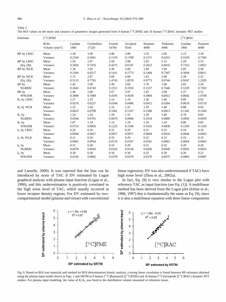
The derivation of the SRTM includes the assumption thatthe free�nonspecific and specific binding compartments arein rapid equilibrium. It is further assumed that there isnegligible specific binding in the reference region. All meth-ods based on SRTM, including nonlinear methods and thelinear methods presented here, will be similarly affected bythe limitations of these assumptions. In addition, the bloodvolume term is ignored in the SRTM, producing a system-atic underestimation of BP regardless of which SRTMmethod is implemented. For example, the BP estimatesobtained by SRTM underestimate the BP estimates obtainedusing a standard two-tissue compartmental model (Fig. 1).The underestimation may result from model simplificationand assumption of the negligible radioactivity of vascularspace in both reference tissue and target tissue. For[11C]FMZ studies, the pons may not be completely devoidof specific receptor binding (Delforge et al., 1997; Price etal., 1993). The correction of the bias due to specific bindingin the reference tissue is usually based on a more complexexperimental protocol with additional scans to estimate BPor nonspecific distribution volume of the reference tissue(Delforge et al., 1997; Lopresti et al., 2001). However, thetheoretical linear relationship verified by our studies (Fig. 8)and other previous studies (Gunn et al., 1997, 2001; Lam-

mertsma and Hume, 1996; Millet al., 2002) demonstratethat SRTM is a reliable quantification method for studyingthe changes in BP induced by psychological stimulation orpharmacological challenges.

The results from computer simulation of [11C]FMZ inthe present study are generally consistent with those ob-tained from human [11C]FMZ PET data. In the computersimulation, we found that high noise in the reference TACcan add both bias and variance to the parameter estimates,especially for a tissue TAC of low noise level. In this study,we also simulated the reference TAC of low noise level (�� 0.01) and found that the effects on estimates is almostnegligible. This suggests that some preprocessing, such assmoothing the reference tissue TAC, may be helpful insome special situations. For example, if the reference TACderived from a small region such as pons is quite noisy dueto movement during PET scan, then movement correctionor temporal smoothing technique, such as fitting mutliex-ponentionals to the reference TACs should be performed.

The operation equations (Eqs. (8) and (9)) are first de-rived to generate parametric images of SRTM. Both com-puter simulation and human studies show that conventionalnonlinear regression with operational Eq. (2) and linearregression with Eq. (8) is comparable for estimating theparameters of SRTM from low noise level of TAC. LRSCis suggested for high noise level of TAC or parametricimaging of SRTM model. Although the BP images gener-ated by WLR with Eq. (9) are of comparable image qualitywith LRSC, which is consistent with their similar variance,the WLR estimates show more bias than LRSC, especiallyfor pixel TAC of high noise level or ROI TAC of lowerreceptor density and small volume. It is worth noting thatthe noise introduced bias (underestimation) was also studiedfor DV estimation in ligand-receptor PET or single-photonemission computed tomography (SPECT) studies (Slifstein

Fig. 7. Pixelwise mean (A) and variance (B) of estimates of R1 (top row), k2 (middle row), and binding potential (BP) (bottom) generated from the nine human[11C]flumazenil ([11C]FMZ) dynamic PET studies. (Left to right) Linear regression with spatial constraint (LRSC), weighted linear regression (WLR),nonlinear ridge regression with spatial constraint (NLRRSC), and weighted nonlinear regression with the Marquardt (WNLRM) algorithm.


and Laruelle, 2000). It was reported that the bias can beintroduced by noise of TAC if DV estimated by Logangraphical analysis with plasma input function (Logan et al.,1990), and this underestimation is positively correlated tothe high noise level of TAC, which usually occurred atlower receptor density regions. For DV estimated by two-compartmental model (plasma and tissue) with conventional

linear regression, DV was also underestimated if TACs havehigh noise level (Zhou et al., 2002a).

In fact, Eq. (9) is very similar to the Logan plot withreference TAC as input function (see Eq. (1)). A multilinearmethod has been derived from the Logan plot (Ichise et al.,1996, 1997) that is fundamentally the same as Eq. (9), sinceit is also a multilinear equation with three linear components

Table 2The ROI values on the mean and variance of parametric images generated from 9 human [11C]FMZ and 16 human [11C]RAC dynamic PET studies

Estimates [11C]FMZ [11C]RAC

ROIs: Caudate Cerebellum Frontal Occipital Putamen Thalamus Caudate PutamenVolume (mm3): 1960 17520 16784 9544 4008 4496 1960 4008

BP by LRSC Mean 1.38 1.99 3.48 3.89 1.55 2.00 2.15 2.39Variance 0.2334 0.5601 0.1374 0.1708 0.1371 0.6353 0.5329 0.7583

BP by LRSC(Eq. (8))

Mean 1.50 2.07 3.58 3.98 1.65 2.12 2.29 2.53Variance 0.3026 0.7476 0.4275 0.6747 0.2653 0.8416 0.7323 1.0051

BP by WLR Mean 1.34 1.92 3.30 3.68 1.49 1.94 2.05 2.28Variance 0.2504 0.6517 0.1421 0.1773 0.1404 0.7397 0.5694 0.8011

BP by WLR(Eq. (8))

Mean 1.15 2.07 3.60 4.00 1.43 2.00 2.28 2.52Variance 0.5113 0.7763 1.4743 1.8578 0.9773 0.8744 0.9247 1.2205

BP byNLRRSC

Mean 1.42 2.00 3.39 3.83 1.70 1.96 2.05 2.26Variance 0.2643 0.6743 0.1551 0.1910 0.1537 0.7646 0.5329 0.7583

BP byWNLRM

Mean 1.46 2.08 3.57 3.97 1.65 2.08 2.27 2.51Variance 0.3890 0.7680 0.4195 0.4538 0.3804 0.8412 0.8042 1.0768

R1 by LRSC Mean 1.27 1.19 1.14 1.19 1.36 1.46 0.85 0.92Variance 0.0276 0.0257 0.0344 0.0486 0.0412 0.0284 0.0674 0.0719

R1 by WLR Mean 1.33 1.20 1.16 1.21 1.39 1.48 0.88 0.92Variance 0.0625 0.0798 0.1061 0.1337 0.1506 0.0813 0.1342 0.1269

R1 byNLRRSC

Mean 1.24 1.24 1.29 1.31 1.30 1.40 0.78 0.83Variance 0.0544 0.0791 0.0670 0.0946 0.1018 0.0889 0.0950 0.0939

R1 byWNLRM

Mean 1.07 1.14 1.14 1.19 1.16 1.24 0.80 0.85Variance 0.0723 0.0826 0.1225 0.1349 0.1616 0.0838 0.1200 0.1183

k2 by LRSC Mean 0.20 0.26 0.32 0.29 0.31 0.23 0.18 0.18Variance 0.0040 0.0027 0.0057 0.0071 0.0044 0.0034 0.0044 0.0045

k2 by WLR Mean 0.21 0.26 0.33 0.29 0.32 0.23 0.19 0.19Variance 0.0081 0.0054 0.0176 0.0197 0.0181 0.0063 0.0064 0.0063

k2 byNLRRSC

Mean 0.31 0.28 0.33 0.29 0.31 0.32 0.20 0.20Variance 0.0078 0.0043 0.0165 0.0136 0.0206 0.0049 0.0055 0.0055

k2 byWNLRM

Mean 0.39 0.30 0.34 0.30 0.32 0.39 0.20 0.21Variance 0.0145 0.0062 0.0378 0.0379 0.0379 0.0075 0.0083 0.0087

Fig. 8. Based on ROI (see materials and method for ROI determination) kinetic analysis, a strong linear correlation is found between BP estimates obtainedusing the plasma input model shown in Figs. 1 and SRTM in 9 human [11C]flumazenil ([11C]FMZ) and 16 human [11C]raclopride ([11C]RAC) dynamic PETstudies. For plasma input modeling, the value of K1/k2 was fixed to the distribution volume measured in reference tissue.


with one of the parameters being DVR. In fact, using refer-ence TAC as input, the Logan plot as well as its variationscan be considered as a special case of SRTM. This can beeasily seen by the following equation resulted from dividingEq. (9) by CT:

�0t CT�s�ds

CT�t�� DVR

�0t CREF�s�ds

CT�t�

� DVR/�k2/R1�CREF�t�

CT�t�� DVR/k2�.

Note that k2R � k2/R1. Thus, for tissue time activity curvesof low noise level, the Logan plot and the Eq. (9) derivedfrom SRTM are fundamentally the same equation for BPestimation. Statistically, the BP estimated using Eq. (9) orthe above equation derived from Logan plot can be consid-ered as a special technique to minimize the variance ofestimates by estimating ratio without division, if it is com-pared to the BP estimated using Eq. (8) (Lange, 1999).Based on conventional ROI kinetic analysis, the Logan plotand SRTM with Eq. (2) provides almost identical estimatesof BP (Sossi et al., 2001). It is expected that the BP is alsounderestimated by Logan plot or its variation (Ichise et al.,1996, 1997), and this underestimation is also due to noise ofTAC and model approximation.

In this study, the parameters estimated by conventionalnonlinear regression using operational Eq. (2) were com-pared to those estimated by linear regression and LRSCusing computer simulation, a lower noise level of ROITACs, and a high noise level of pixel TAC. At the lowernoise level of simulated data or ROI TACs, all methods givealmost same estimates. Nonlinear regression is very sensi-tive to the noise level of tissue TAC, which can result inintrinsic nonlinear problems such as local minimums andconvergence, nonlinear estimators can also become biasedestimators at a high noise level of TACs. In this study wehave demonstrated that the linear estimator is more accuratethan a nonlinear estimator although there is a small biascontributed from integration into the linear estimator. Wealso found that the accuracy of conventional WLR estimatesof R1 and k2 is markedly improved by general ridge regres-sion with spatial constraint. It is necessary to clarify, how-ever, that greater accuracy of parameter estimates does notnecessarily correspond to the best fit of measured TAC. Infact a better fit, as judged by a lower residual sum square inkinetic space, is usually at the cost of higher spatial varia-tion in parameter space (Zhou et al., 2002c).

When applying the linear GRRSC algorithm used inLRSC, a high-pass filter is recommended to be used in thefiltered backprojection reconstruction to maintain high spa-tial resolution in the dynamic images. This ensures optimaltrade-off between noise depression and spatial resolutionloss that can be produced by GRRSC when generating

parametric images. In addition, the spatial smoothing filter(equal weighting over all pixels within given window inplane) selected for LRSC in the current study originatedfrom the criterion of minimizing local variation in the para-metric image. In fact, any filter could be used in the LRSC,and its selection is always dependent on the noise level ofthe dynamic images. Note that LRSC is not sensitive to thesmoothing filter, and this is consistent with results obtainedin our previous studies (Zhou et al., 2001, 2002a, 2002b,2002c). Although the smoothing filter for spatial constraintis the same for the parametric image generation algorithmsusing Eqs. (8) and (9) of LRSC, they have different effectson the parametric images. For R1 and k2, the spatial con-straint is automatically adjusted by both the variance ofpixel kinetics and the variance of estimates, based on theGRRSC theory. Therefore, the resolution loss of R1 and k2

images due to spatial constraint is not spatially uniform, andthe k2 images have lower spatial resolution. For the BP, theselection of the applied smoothing filter is somewhat arbi-trary. However, based on the theory (see subsection “Para-metric image generation algorithm using Eq. (9)”), and theresults (WLR versus LRSC) of computer simulations andhuman studies, the BP estimates obtained with LRSC arequite robust to the spatial constraint in terms of the varianceand resolution loss. In fact, the results from human studiesdemonstrate that the resolution of BP images generated byLRSC and WLR is visually comparable. Additionally, BPobtained using Eq. (9) is not sensitive to the weighting forlinear regression, since the output measurements �0

tCT�s�dsis of low noise level (see Materials and methods). Note thatthe regression weighting for model fitting is chosen to beproportional to the scan length in the present study. Strictlyspeaking, Wii, as chosen in our computer simulation, shouldbe related to the scan length of the frame and is inverselyrelated to the average counts in the frame for parameterestimation using Eq. (2) or Eq. (8) (Chen et al., 1991). Inpractice, however, we find that the use of the scan length toapproximate Wii gives good and robust results for generat-ing parametric images (Zhou et al., 2001, 2002a, 2002b,2002c).

In summary, in contrast to nonlinear regression using Eq.(2), utilization of the operational Eqs. (8) and (9) of integralform derived from a simplified reference tissue model aresimpler, more robust, and more computationally efficientfor parameter estimation. For LRSC, results from computersimulations and human studies show that the variance ofestimates is reduced by ridge regression while the bias ofestimates is limited by the spatial constraint. This finding isconsistent with ridge regression theory (Hoerl and Kennard,1970a, 1970b), and the results obtained in the previousstudies (Zhou et al., 2001, 2002c). We conclude that thenew linear equations yield a reliable, computationally effi-cient, and robust LRSC algorithm that is suggested to gen-erate parametric images of ligand-receptor dynamic PETstudies with SRTM.


Acknowledgments

We thank the cyclotron, PET, and MRI imaging staff ofthe Johns Hopkins Medical Institutions; Abdul Kalaff andLauren Sims for subject recruitment and data collection;Andrew H. Crabb for data acquisition and computer sup-port; and Dr. John Hilton for HPLC metabolite analysis.This work was partially supported by USPHS Grants(D.F.W.) MH42821, AA12839, DA11080, DA09482,DA00412, HD24448, and NS38927; the Essel Foundation;Family and Friends of Chelsea Coenraads; the NationalAlliance for Research on Schizophrenia and Depression(NARSAD); and the Rett Syndrome Research Foundation(RSRF).

References

Banati, R.B., Goerres, G.W., Myers, R., Gunn, R.N., Turkheimer, F.E.,Kreutzberg, G.W., Brooks, D.J., Jones, T., Duncan, J.S., 1999.[11C](R)-PK11195 positron emission tomography imaging of activatedmicroglia in vivo in Rasmussen’s encephalitis. Neurology 53, 2199–2203.

Blomqvist, G., 1984. On the construction of functional maps in positronemission tomography. J. Cereb. Blood Flow Metab. 4, 629–623.

Blomqvist, G., Pauli, S., Farde, L., Eriksson, L., Persson, A., Halldin, C.,1990. Maps of receptor binding parameters in the human brain—akinetic analysis of PET measurements. Eur. J. Nucl. Med. 16, 257–265.

Blomqvist, G., Tavitian, B., Pappata, S., Crouzel, D., Jobert, A., Doignon,I., Di Giamberardino, L., 2001. A tracer kinetic model for measurementof regional acetylcholinesterase activity in the brain using [11C]phy-sostigmine and PET, in: Gjedde, A., Hansen, S.B., Knudsen, G.M.,Paulson, O.B. (Eds.), Physiological Imaging of the Brain with PET,Academic Press, San Diego, pp. 273–278.

Carson, R.E., Channing, M.A., Blasberg, R.G., Dunn, B.B., Cohen, R.M.,Rice, K.C., Herscovitch, P., 1993. Comparison of bolus and infusionmethods for receptor quantitation: application to [18F]cyclofoxy andpositron emission tomography. J. Cereb. Blood Flow Metab. 13, 24–42.

Carson, R.E., Huang, S.-C., Green, M.V., 1986. Weighted integrationmethod for local cerebral blood flow measurements with positronemission tomography. J. Cereb. Blood Flow Metab. 16, 245–258.

Chen, K., Huang, S.C., Yu, D.C., 1991. The effects of measurement errorsin the plasma radioactivity curve on parameter estimation in positronemission tomography. Phys. Med. Biol. 36, 1183–1200.

Chen, K., Lawson, M., Reiman, E., Cooper, A., Feng, D., Huang, S.C.,Bandy, D., Ho, D., Yun, L.S., Palant, A., 1998. Generalized linear leastsquares method for fast generation of myocardial blood flow parametricimages with N-13 ammonia PET. IEEE Trans. Med. Imag. 17, 236–243.

Cherry, S.R., Meikle, S.R., Hoffman, E.J., 1993. Correction and charac-terization of scattered events in three-dimensional PET using scannerswith retractable septa. J. Nucl. Med. 34, 671–678.

Delforge, J., Spelle, L., Bendriem, S.B., Samson, Y., Syrota, A., 1997.Parametric images of benzodiazepine receptor concentration using apartial-saturation injection. J. Cereb. Blood Flow Metab. 17, 343–355.

Endres, C.J., Carson, R.E., 1998. Assessment of dynamic neurotransmitterchanges with bolus or infusion delivery of neuroreceptor ligands.J. Cereb. Blood Flow Metab. 18, 1196–1210.

Evans, A.C., Marrett, S., Torrescorzo, J., Ku, S., Collins, L., 1991. MRI-PET correlation in three dimensions using a volume-of-interest (VOI)atlas. J. Cereb. Blood Flow Metab. 11, A69–A78.

Farde, L., Eriksson, L., Blomquist, G., Halldin, C., 1989. Kinetic analysisof central [11C]raclopride binding to D2-dopamine receptors studied by

PET—a comparison to the equilibrium analysis. J. Cereb. Blood FlowMetab. 9, 696–708.

Feng, D., Wong, Z., Huang, S.C., 1993. A study on statistically reliable andcomputationally efficient algorithms for generating local cerebral bloodflow parametric images with positron emission tomography. IEEETrans. Med. Imag. 12, 182–188.

Frost, J.J., Douglass, K.H., Mayberg, H.S., Dannals, R.F., Links, J.M.,Wilson, A.A., Ravert, H.T., Crozier, W.C., Wagner Jr., H.N., 1989.Multicompartmental analysis of [11C]-carfentanil binding to opiatereceptors in humans measured by positron emission tomography.J. Cereb. Blood Flow Metab. 9, 398–409.

Ginovart, N., Wilson, A.A., Meyer, J.H., Hussey, D., Houle, S., 2001.Positron emission tomography quantification of [11C]-DASB bindingto the human sertonin transporter: modeling strategies. J. Cereb. BloodFlow Metab. 21, 1342–1353.

Gunn, R.N., Gunn, S.R., Cunningham, V.J., 2001. Positron emission to-mography compartmental models. J. Cereb. Blood Flow Metab. 21,635–652.

Gunn, R.N., Lammertsma, A.A., Hume, S.P., Cunningham, V.J., 1997.Parametric imaging of ligand-receptor binding in PET using a simpli-fied reference region model. NeuroImage 6, 279–287.

Gunn, R.N., Sargent, P.A., Bench, C.J., Rabiner, E.A., Osman, S., Pike,V.W., Hume, S.P., Grasby, P.M., Lammertsma, A.A., 1998. Tracerkinetic modeling of the 5-HT1A receptor ligand [carbonyl-11C]WAY-100635 for PET. NeuroImage 8, 426–440.

Herholz, K., 1987. Nonstational spatial filtering and accelerated curvefitting for parametric imaging with dynamic PET. Eur. J. Nucl. Med.14, 477–484.

Hoerl, A.E., Kennard, R.W., 1970a. Ridge regression: applications tononorthogonal problems. Technometrics 12, 69–82.

Hoerl, A.E., Kennard, R.W., 1970b. Ridge regression: biased estimationfor nonorthogonal problems. Technometrics 12, 55–67.

Holden, J.E., Sossi, V., Chan, G., Doudet, D.J., Stoessl, A.J., Ruth, T.J.,2001. Effect of population k2 values in graphical estimation of DVratios of reversible ligands, in: Gjedde, A., Hansen, S.B., Knudsen,G.M., Paulson, O.B. (Eds.), Physiological Imaging of the Brain withPET, Academic Press, San Diego, pp. 127–129.

Huang, S.-C., Zhou, Y., 1998. Spatially-coordinated regression for image-wise model fitting to dynamic PET data for generating parametricimages. IEEE Trans. Nucl. Sci. 45, 1194–1199.

Ichise, M., Ballinger, J.R., Golan, H., et al., 1996. Noninvasive quantifi-cation of dopamine D2-receptors with iodine-123-IBF SPECT. J. Nucl.Med. 37, 513–520.

Ichise, M., Ballinger, J.R., Vines, D., Tsai, S., Kung, H.F., 1997. Simplifiedquantification and reproducibility studies of dopamine D2-receptorbinding with Iodine-123-IBF SPECT in health subjects. J. Nucl. Med.38, 31–37.

Kimura, Y., Senda, M., Alpert, N.M., 2002. Fast formation of statisticallyreliable FDG parametric images based on clustering and principalcomponents. Phys. Med. Biol. 47, 455–68.

Koeppe, R.A., Holthoff, V.A., Frey, K.A., Kilbourn, M.R., Kuhl, D.E.,1991. Compartmental analysis of [11C]flumazenil kinetics for the esti-mation of ligand transport rate and receptor distribution using positronemission tomography. J. Cereb. Blood Flow Metab. 11, 735–744.

Koeppe, R.A., Frey, K.A., Vander Borght, T.M., Karlamangla, A., Jewett,D.M., Lee, L.C., Kilbourn, M.R., Kuhl, D.E., 1996. Kinetic evaluationof [11C]dihydrotetrabenazine by dynamic PET: measurement of vesic-ular monoamine transporter. J. Cereb. Blood Flow Metab. 16, 1288–1299.

Lammertsma, A.A., Bench, C.J., Hume, S.P., Osman, S., Gunn, K.,Brooks, D.J., Frackowiak, R.S.J., 1996. Comparison of methods foranalysis of clinical [11C]raclopride studies. J. Cereb. Blood FlowMetab. 16, 42–52.

Lammertsma, A.A., Hume, S.P., 1996. Simplified reference tissue modelfor PET receptor studies. NeuroImage 4, 153–158.

Lange, K., 1999. Numerical Analysis for Statisticians. Springer-Verlag,New York.


Lassen, N.A., Bartenstein, P.A., Lammertsma, A.A., Prevett, M.C., Turton,D.R., Luthra, S.K., Osman, S., Bloomfield, P.M., Jones, T., Patsalos,P.N., O’Connell, M.T., Duncan, J.S., Vanggaard Andersen, J., 1995.Benzodiazepine receptor quantification in vivo in humans using[11C]flumazenil and PET: application of the steady-state principal.J. Cereb. Blood Flow Metab. 15, 152–165.

Lawton, W.H., Sylvestre, E.A., 1971. Elimination of linear parameters innonlinear regression. Technonmetrics 13, 461–467.

Logan, J., Fowler, J.S., Volkow, N.D., et al., 1990. Graphical analysis ofreversible radioligand binding from time-activity measurements ap-plied to [N-11C-methuyl]-(�)-cocaine PET studies in human subjects.J. Cereb. Blood Flow Metab. 10, 740–747.

Logan, J., Fowler, J.S., Volkow, N.D., Wang, G-J., Ding, Y-S., Alexoff,D.L., 1996. Distribution volume ratios without blood sampling fromgraphic analysis of PET data. J. Cereb. Blood Flow Metab. 16, 834–840.

Lopresti, B.J., Mathis, C.A., Price, J.C., Villemagne, V., Meltzer, C.C.,Holt, D.P., Smith, G.S., Moore, R.Y., 2001. Serotonin transporterbinding in vivo: further examination of [11C]McN5652, in: Gjedde, A.,Hansen, S.B., Knudsen, G.M., Paulson, O.B. (Eds.), PhysiologicalImaging of the Brain with PET, Academic Press, San Diego, pp.265–271.

Marquardt, D.W., 1963. An algorithm for least-squares estimations ofnonlinear parameters. J. Soc. Ind. Appl. Math. 11, 431–441.

Millet, P., Graf, C., Buck, A., Walder, B., Ibanez, V., 2002. Evaluation ofthe reference tissue models for PET and SPECT benzodiazepine bind-ing parameters. NeuroImage 17, 928–942.

Mintun, M.A., Raichle, M.E., Kilbourn, M.R., Wooten, G.F., Welch, M.J.,1984. A quantitative model for the in vivo assessment of drug bindingsites with positron emission tomography. Ann Neurol. 15, 217–227.

O’Sullivan, F., 1994. Metabolic images from dynamic positron emissiontomography studies. Stat. Methods Med. Res. 3, 87–101.

Parsey, R.V., Slifstein, M., Hwang, D.-R., Abi-Dargham, A., Simpson, N.,Guo, N., Shinn, A., Mawlawi, O., Van Heertum, R., Mann, J.J., Laru-elle, M., 2001. Comparison of kinetic modeling methods for the in vivoquantification of 5-HT1A receptors using WAY 100635, in: Gjedde, A.,Hansen, S.B., Knudsen, G.M., Paulson, O.B. (Eds.), PhysiologicalImaging of the Brain with PET, Academic Press, San Diego, pp.249–255.

Patlak, C.S., Blasberg, R.G., 1985. Graphical evaluation of blood-to-braintransfer constants from multiple-time uptake data: generalizations.J. Cereb. Blood Flow Metab. 5, 584–590.

Price, J.C., Mayberg, H.S., Dannals, R.F., Wilson, A.A., Ravert, H.T.,Sadzot, B., Rattner, Z., Kimball, A., Feldman, M.A., Frost, J.J., 1993.Measurement of benzodiazepine receptor number and affinity in hu-mans using tracer kinetic modeling, positron emission tomography, and[11C]flumazenil. J. Cereb. Blood Flow Metab. 13, 656–667.

Slifstein, M., Laruelle, M., 2000. Effects of statistical noise on graphicanalysis of PET neuroreceptor studies. J. Nucl. Med. 41, 2083–2088.

Sossi, V., Holden, J.E., Chan, G., Krzywinski, M., Stoessl, A.J., Ruth, T.J.,2001. Measuring the BP of four dopaminergic tracers utilizing a tissueinput function, in: Gjedde, A., Hansen, S.B., Knudsen, G.M., Paulson,O.B. (Eds.), Physiological Imaging of the Brain with PET, AcademicPress, San Diego, pp.131–137.

Szabo, Z., Scheffel, U., Mathews, W.B., Ravert, H.T., Szabo, K., Kraut,M., Palmon, S., Ricaurte, G.A., Dannals, R.F., 1999. Kinetic analysisof [11C]McN5652: a serotonin transporter radioligand. J. Cereb. BloodFlow Metab. 19, 967–981.

Wagner Jr., H.N., Burns, H.D., Dannals, R.F., Wong, D.F., Langstrom, B.,Duelfer, T., Frost, J.J., Ravert, H.T., Links, J.M., Rosenbloom, S.B.,Lukas, S.E., Kramer, A.V., Kuhar, M.J., 1983. Imaging dopaminereceptors in the human brain by positron emission tomography. Science221, 1264–1266.

Wong, D.F., Wagner Jr., H.N., Dannals, R.F., et al., 1984. Effects of ageon dopamine and serotonin receptors measured by positron tomographyin the living human brain. Science 226, 1393–1396.

Wong, D.F., Yung, B., Dannals, R.F., Shaya, E.K., Ravert, H.T., Chen,C.A., Chan, B., Folio, T., Scheffel, U., Ricaurte, G.A., Neumeyer, J.L.,Wagner Jr., H.N., Kuhar, M.J., 1993. In vivo imaging of baboon andhuman dopamine transporters by positron emission tomography using[11C]WIN35,428. Synapse 15, 130–142.

Zhou, Y., Huang, S.C., Bergsneider, M., 2001. Linear ridge regression withspatial constraint for generation of parametric images in dynamicpositron emission tomography studies. IEEE Trans. Nucl. Sci. 48,125–130.

Zhou, Y., Brasic, J.R., Musachio, J.L., et al., 2002a. Human [123I]5-I-A-85380 dynamic SPECT studies in normals: kinetic analysis and para-metric imaging. Proc. IEEE Nucl. Sci. Symp. Med. Imag. 1335–1340.

Zhou, Y., Huang, S.C., Bao, S., Wong, D.F., 2002b. Parametric imagingand statistical mapping of brain tumor in Ga-68 EDTA dynamic PETstudies. Proc. IEEE Nucl. Sci. Symp. Med. Imag. 1072–1078.

Zhou, Y., Huang, S.C., Bergsneider, M., Wong, D.F., 2002c. Improvedparametric image generation using spatial-temporal analysis of dy-namic PET studies. NeuroImage 15, 697–707.


Linear regression with spatial constraint to generate...

Documents

Transcript of Linear regression with spatial constraint to generate...