IMF Country Report No. 15/314 MEXICO Country Report No. 15/314 MEXICO SELECTED ISSUES This Selected...
84
© 2015 International Monetary Fund IMF Country Report No. 15/314 MEXICO SELECTED ISSUES This Selected Issues paper on Mexico was prepared by a staff team of the International Monetary Fund as background documentation for the periodic consultation with the member country. It is based on the information available at the time it was completed on October 23, 2015. Copies of this report are available to the public from International Monetary Fund Publication Services PO Box 92780 Washington, D.C. 20090 Telephone: (202) 623-7430 Fax: (202) 623-7201 E-mail: [email protected] Web: http://www.imf.org Price: $18.00 per printed copy International Monetary Fund Washington, D.C. November 2015
Transcript of IMF Country Report No. 15/314 MEXICO Country Report No. 15/314 MEXICO SELECTED ISSUES This Selected...

© 2015 International Monetary Fund
IMF Country Report No. 15/314
MEXICO SELECTED ISSUES
This Selected Issues paper on Mexico was prepared by a staff team of the International
Monetary Fund as background documentation for the periodic consultation with the
member country. It is based on the information available at the time it was completed on
October 23, 2015.
Copies of this report are available to the public from
International Monetary Fund Publication Services
PO Box 92780 Washington, D.C. 20090
Telephone: (202) 623-7430 Fax: (202) 623-7201
E-mail: [email protected] Web: http://www.imf.org
Price: $18.00 per printed copy
International Monetary Fund
Washington, D.C.
November 2015

MEXICO SELECTED ISSUES
Approved By Robert Rennhack
Prepared By Juliana D. Araujo, Marcos Chamon, Julian Chow,
Alexander Klemm, Alexander Herman, and Fabian Valencia
FISCAL MULTIPLIERS IN MEXICO _______________________________________________________ 4
A. Inferring Fiscal Multipliers from State-Level Public Spending __________________________ 4
B. Estimation Results ______________________________________________________________________ 5
C. State-Dependent Fiscal Multipliers _____________________________________________________ 7
D. Growth Implications from the Fiscal Consolidation ____________________________________ 8
E. Conclusions ____________________________________________________________________________ 9
References _______________________________________________________________________________ 10
TRADE AND FINANCIAL SPILLOVERS TO MEXICO ____________________________________11
A. Introduction __________________________________________________________________________ 11
B. Trade Linkages ________________________________________________________________________ 12
C. Financial Linkages _____________________________________________________________________ 13
D. The Impact of Foreign and Domestic Factors on GDP_________________________________ 15
E. A Closer Look at Changes in Monetary Conditions in the U.S. _________________________ 18
F. Conclusions ___________________________________________________________________________ 18
References _______________________________________________________________________________ 20
FIGURE
1. Response to a 100-bps Shock in 10-Year U.S. Bond Yield _____________________________ 19
APPENDICES
I. Historical Decomposition of Real GDP Growth _________________________________________ 22
II. Impulse Responses (Section D) ________________________________________________________ 23
II. Impulse Responses (Section E) ________________________________________________________ 24
CONTENTS
October 23, 2015

MEXICO
2 INTERNATIONAL MONETARY FUND
CORPORATE VULNERABILITIES AND IMPACT ON THE REAL ECONOMY ____________________24
A. Rising Corporate Debt ________________________________________________________________________ 24
B. Vulnerabilities _________________________________________________________________________________ 27
C. Stress Tests ___________________________________________________________________________________ 29
D. Impact on the Banking Sector ________________________________________________________________ 32
E. Impact on the Real Economy __________________________________________________________________ 33
F. Summary and Conclusion _____________________________________________________________________ 35
References _______________________________________________________________________________________ 39
APPENDIX
I. Methodology for Corporate Sensitivity Analysis _______________________________________________ 36
FIGURES
1. Corporate Debt _______________________________________________________________________________ 25
2. Corporate Leverage ___________________________________________________________________________ 26
3. Corporate Credit Metrics ______________________________________________________________________ 28
4. Corporate Sensitivity Analysis _________________________________________________________________ 30
5. Impact on the Banking Sector _________________________________________________________________ 32
BOX
1. Interest Coverage Ratio and Debt at Risk _____________________________________________________ 31
A CARBON TAX PROPOSAL FOR MEXICO _____________________________________________________41
A. Introduction ___________________________________________________________________________________ 41
B. Mexico’s Current Excise Taxes on Fossil Fuels _________________________________________________ 42
C. In Search for a New Energy Taxation Mechanism _____________________________________________ 43
D. Estimating Optimal Carbon Tax Rates on Fossil Fuels for Mexico _____________________________ 44
E. Impact of Imposing Carbon Tax Rates _________________________________________________________ 49
F. Conclusions ___________________________________________________________________________________ 50
References _______________________________________________________________________________________ 51
STRENGTHENING MEXICO’S FISCAL FRAMEWORK___________________________________________52
A. Introduction ___________________________________________________________________________________ 52
B. Mexico’s Fiscal Framework: Recent Improvements and Pending Tasks ________________________ 53
C. Dealing with Exceptional Circumstances ______________________________________________________ 55
D. A New Nominal Anchor _______________________________________________________________________ 56
E. Fiscal Council __________________________________________________________________________________ 59
F. Conclusions ___________________________________________________________________________________ 60
References _______________________________________________________________________________________ 61

MEXICO
INTERNATIONAL MONETARY FUND 3
FIGURE
1. Probability Distribution of Public Debt Under Different PSBR Ceilings __________________________ 58
BOXES
1. The Fiscal Responsibility Law: Main Features __________________________________________________ 54
2. Examples of Fiscal Rules with Explicit Debt Ceilings ___________________________________________ 57
3. Examples of Fiscal Council Mandates __________________________________________________________ 60
THE EFFECTS OF FX INTERVENTION IN MEXICO ______________________________________________62
A. Introduction ___________________________________________________________________________________ 62
B. Peso Response in the Aftermath of Changes to FX Intervention Policy ________________________ 62
C. Concluding Remarks __________________________________________________________________________ 68
References _______________________________________________________________________________________ 69
FIGURES
1. Evolution of the Exchange Rate vis-a-vis U.S. Dollar Around Foreign Exchange Intervention
Program Announcement Dates __________________________________________________________________ 63
2. Evolution of Option-Implied Exchange Rate Volatility Around Foreign Exchange Intervention
Program Announcement Dates __________________________________________________________________ 64
FINANCIAL DEEPENING IN MEXICO ___________________________________________________________70
A. Motivation ____________________________________________________________________________________ 70
B. Credit Depth in Mexico ________________________________________________________________________ 73
C. Reasons for the Low Level of Financial Intermediation ________________________________________ 75
D. Current Trends and Policies ___________________________________________________________________ 79
E. Conclusions ___________________________________________________________________________________ 81
References _______________________________________________________________________________________ 82
FIGURES
1. Bank Loans to Enterprises _____________________________________________________________________ 72
2. Marginal Interest Rates ________________________________________________________________________ 77

MEXICO
4 INTERNATIONAL MONETARY FUND
FISCAL MULTIPLIERS IN MEXICO1
As fiscal consolidation begins in Mexico, the question of the size of fiscal multipliers becomes highly
relevant. Estimates of fiscal multipliers––obtained from state-level spending––fall within 0.6–0.7 after
accounting for dynamic effects. However, the size of multipliers varies with the output gap. Point
estimates for the cumulative multiplier can exceed one when the output gap is sufficiently negative,
while they decline and even turn statistically insignificant when the output gap is above 0.5 percent.
The planned fiscal consolidation—under the estimated multipliers—is projected to subtract on average
½ percentage points from growth over 2015–2020. However, there are offsetting effects. The
consolidation is partly a consequence of lower oil prices, which have helped bring down electricity
prices. The positive growth impulse of lower costs on manufactured goods production is estimated to
reach ½ percentage point in 2015 and 2016, largely offsetting the impact of fiscal consolidation on
growth in the near term.
A. Inferring Fiscal Multipliers from State-Level Public Spending
1. Mexico established the Fiscal Coordination System (FCS) in 1980 with the main goal of
harmonizing public finances. Each state signed agreements with the treasury of the Federation
adhering to the FCS. Adherence implied that the states would get a share in revenues collected by
the Federal Government—“Participaciones”—in exchange for eliminating or suspending local taxes
that were deemed incompatible with the newly created VAT. In 1997, Mexico expanded the system
of federal transfers to accommodate a de-centralization of federal activities, including in the areas of
basic education, health, social infrastructure, and security. These decentralized responsibilities are
financed through a system of earmarked transfers—“Aportaciones”—to states and municipalities.
2. After the FCS, Federal transfers have represented a large fraction of state-level fiscal
revenues—about 90 percent over the last two decades--and are therefore little influenced by
local economic conditions. This institutional setting allows the estimation of fiscal multipliers with
reduced concerns about reverse causality—by which causality would go from growth to spending
and not the other way around—often an important econometric obstacle.2 This is confirmed in
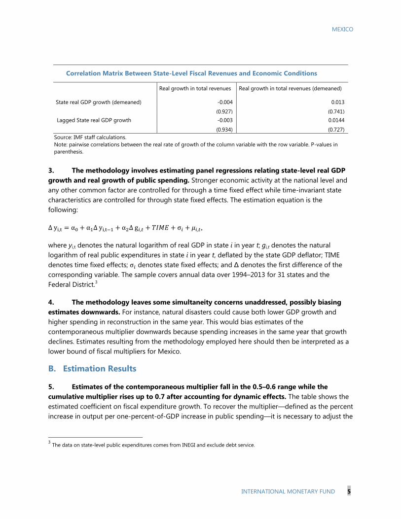
simple correlations between the real growth in total revenues with state real GDP growth, which are
statistically insignificant.
1 Prepared by Fabian Valencia. The author thanks Ivan Arias, Marcos Chamon, Alex Klemm, Dora Iakova, Petia
Topalova, and seminar participants at the Mexican Ministry of Finance and the Central Bank of Mexico for insightful
comments and suggestions and Alexander Herman for outstanding research assistance.
2 Blanchard and Perotti (2002) argued that when using annual data, it is more likely to run into reverse causality
concerns because discretionary spending has had time to adjust to changes in real GDP growth. If this is the case,
fiscal revenues at the state level would be correlated with local economic conditions—so that expenditures adjust in
anticipation to higher revenues derived from better economic conditions. However, weak historical correlations
between state fiscal revenues and local real GDP growth reduce concerns about this problem.
MEXICO
INTERNATIONAL MONETARY FUND 5
Correlation Matrix Between State-Level Fiscal Revenues and Economic Conditions
Real growth in total revenues Real growth in total revenues (demeaned)
State real GDP growth (demeaned) -0.004 0.013
(0.927) (0.741)
Lagged State real GDP growth
(demeaned)
-0.003 0.0144
(0.934) (0.727)
Source: IMF staff calculations.
Note: pairwise correlations between the real rate of growth of the column variable with the row variable. P-values in
parenthesis.
3. The methodology involves estimating panel regressions relating state-level real GDP
growth and real growth of public spending. Stronger economic activity at the national level and
any other common factor are controlled for through a time fixed effect while time-invariant state
characteristics are controlled for through state fixed effects. The estimation equation is the
following:
,
where yi,t denotes the natural logarithm of real GDP in state i in year t; gi,t denotes the natural
logarithm of real public expenditures in state i in year t, deflated by the state GDP deflator; TIME
denotes time fixed effects; denotes state fixed effects; and Δ denotes the first difference of the
corresponding variable. The sample covers annual data over 1994–2013 for 31 states and the
Federal District.3
4. The methodology leaves some simultaneity concerns unaddressed, possibly biasing
estimates downwards. For instance, natural disasters could cause both lower GDP growth and
higher spending in reconstruction in the same year. This would bias estimates of the
contemporaneous multiplier downwards because spending increases in the same year that growth
declines. Estimates resulting from the methodology employed here should then be interpreted as a
lower bound of fiscal multipliers for Mexico.
B. Estimation Results
5. Estimates of the contemporaneous multiplier fall in the 0.5–0.6 range while the
cumulative multiplier rises up to 0.7 after accounting for dynamic effects. The table shows the
estimated coefficient on fiscal expenditure growth. To recover the multiplier—defined as the percent
increase in output per one-percent-of-GDP increase in public spending—it is necessary to adjust the
3 The data on state-level public expenditures comes from INEGI and exclude debt service.

MEXICO
6 INTERNATIONAL MONETARY FUND
coefficient for the share of public spending in GDP.4 The adjustment leads to a contemporaneous
multiplier between 0.5 and 0.6, with the cumulative multiplier peaking between 0.6 and 0.7 by the
third year after accounting for dynamic effects—small autoregressive coefficients imply negligible
effects after the third year. The table shows stable coefficients under different specifications—
including when the sample is restricted to after 2003, when a new system of national accounts was
introduced.
Baseline Results
(1) (2) (3) (4) (5)
Dep. Variable: Sample period: 1994-2013 2003-2013
Fixed Effects GMM 0.158 0.121 0.115 0.116 0.169
(0.070)** (0.047)*** (0.049)** (0.048)** (0.060)***
0.060
(0.044)
0.039 0.046 0.046 0.042 0.035
(0.010)*** (0.010)*** (0.012)*** (0.012)*** (0.014)**
0.008 0.014
(0.015) (0.014)
0.039 0.050 -0.082 0.007 -0.001
(0.009)*** (0.006)*** (0.015)*** (0.004)* (0.004)
Time fixed effects Yes Yes Yes Yes Yes
Fiscal multiplier 1/
Contemporaneous 0.53 0.62 0.62 0.57 0.47
Cumulative (t,t+3) 0.63 0.71 0.70 0.64 0.57
R
2 0.73
N 551 532 551 522 308
Source: IMF staff calculations.
Note: Column 1 reports fixed effects regressions. Columns (2)-(5) report GMM regressions using Blundell and Bond (1998)
estimator. * p<0.1; ** p<0.05; *** p<0.01. Robust standard errors in parentheses.
1 / Obtained from multiplying the coefficient on the real growth of fiscal spending by the inverse of the share of fiscal
spending in GDP (1/0.074=13.5).
6. The estimated multipliers are within the range of values found in many studies. To put
the estimates above into perspective, the table below shows selected studies with the
corresponding estimated multipliers. Differences cannot be attributed only to country heterogeneity
since endogeneity is dealt with differently across studies. For instance, several of the cited studies
focus on defense spending because it is not related to local or national economic conditions to get
around the reverse causality problem.
4 The average value for state fiscal spending in the sample is 7.4 percent of GDP. To obtain the fiscal multiplier, the coefficients
must be multiplied by 1/0.074=13.5.

MEXICO
INTERNATIONAL MONETARY FUND 7
Selected Empirical Estimates of Fiscal Spending Multipliers
Study Multiplier estimate Description
Time-series Studies Based on Defense Spending
Barro (1984) ≈ 0.6 U.S. defense spending increases in
WWI, WWII, Korean War.
Ramey (2011) 0.6-1.2 U.S. defense spending, 1939-2008,
short-run versus long-run.
Barro and Redlick (2011) 0.4-0.8 U.S. defense spending, 1917-2006,
short- run versus long-run.
Hall (2009) ≈ 0.5 U.S. defense spending, 1930-2008.
Owyang, Ramey, Zubairy (2013) ≈ 0.6-0.9 U.S. (1890-2010) and Canada (1922-
2011) defense spending.
Time-series Studies Based on Aggregate Spending
Blanchard and Perotti (2002) 0.6-1.8 (peak) U.S. government expenditure over
1947-1997.
Auerbach and Gorodnichenko
(2012)
-0.33 (cumulative, expansion)
2.24 (cumulative, recession)
U.S. government expenditure over
1947-2008
Panel-data or Cross-sectional Studies
Kraay (2014) 0.5-0.7 Uses timing of World Bank loan
disbursements to 29 developing
countries, 1985-2009, short-run.
Nakamura and Steinsson (2014) ≈ 1.5 U.S. defense spending across U.S.
states, 1966-2006, responses of
state real GDP over two years.
Blanchard and Leigh (2013) >=0.8 Europe
0.5-1 advanced economies
Fraction of growth forecasts errors
explained by change in fiscal stance.
C. State-Dependent Fiscal Multipliers
7. Multipliers can exceed one when the output gap is sufficiently negative, but can turn
statistically insignificant when the output gap is positive. Consistent with findings in the
academic literature—for instance, Auerbach and Gorodnichenko (2012)—the multipliers in Mexico
can vary depending on the level of the output gap.5 The table below shows the baseline regression
augmented with the interaction between the lagged output gap at the state level6 (column 1) and at
the national level (column 2) with the real growth of public spending. The coefficient on the
interaction in both regressions is negative and statistically significant, implying that the more
positive the output gap, the lower the fiscal multiplier, and viceversa. The point estimate for the
contemporaneous multiplier—shown graphically below— is around 1 for values of the output gap
between -2 and -1 percent of potential output, around 0.5 for values of the output gap closer to
5 One of the arguments for the multiplier to vary over the business cycle is the presence of excess capacity during
downturns which reduces the crowding out of private investment following a government spending shock. To
mitigate reverse causality concerns derived from the endogeneity of the output gap—as argued by Baum and others,
2012––we include in the regression the lag of the output gap at the state level, but also check if the results hold
when the national output gap is included, which is much less likely to drive state level fiscal spending.
6 Output gaps at the state level are computing using the HP-filter, applying the same smoothing coefficient to all the series.

MEXICO
8 INTERNATIONAL MONETARY FUND
zero, and statistically insignificantly different from zero when the output gap is 0.5 percent or larger.
The cumulative multiplier shows a similar pattern, with point estimates of up to 1.5 when the output
gap is -2 percent—although not statistically significantly different from one.
State-Dependent Regressions
GMM
Dep. Variable:
State output gap National output
gap
0.311 0.130
(0.048)*** (0.049)***
0.030 0.027
(0.013)** (0.013)**
-0.022 -0.004
(0.003)*** (0.002)**
-0.032 -0.108
(0.010)*** (0.014)***
Time fixed effects Yes Yes
N 532 532
Source: IMF staff calculations.
Note: GMM regressions using Blundell and Bond (1998) estimator. *
p<0.1; ** p<0.05; *** p<0.01. Robust standard errors in parenthesis.
Contemporaneous and Cumulative State-Dependent Fiscal Multipliers
a) Contemporaneous multiplier b) Cumulative over t-t+3
Source: IMF staff calculations.
Note: Multipliers are constructed using the regression with state-level output gaps interacted with changes in real public
expenditure, after adjusting the regression coefficients for the share of public spending in GDP. 95-percent confidence
bands are shown in red (dashed lines).
D. Growth Implications from the Fiscal Consolidation
8. The planned fiscal consolidation would subtract from growth close to ½ percentage
points over 2015–2020 on average. For 2015, the projected reduction of ½ percent of GDP in the
PSBR stems in part from a better-than-expected yield of the 2013 tax reform, which should have
only a marginal impact on growth as its effect on private investment and consumption decisions
-.5
0.5
11.5
-2.5 -2 -1.5 -1 -.5 0 .5 1 1.5 2 2.5Output gap
-10
12
-2.5 -2 -1.5 -1 -.5 0 .5 1 1.5 2 2.5Output gap

MEXICO
INTERNATIONAL MONETARY FUND 9
must have taken place before 2015. The negative growth impulse for 2015–16 is related to the
significant compression of primary expenditure in these years. The drag on growth, however, should
diminish over the medium term, as reductions in spending moderate and the output gap closes.
9. As consolidation is in part driven by lower oil prices, its impact on growth is largely
offset by the positive effects of lower energy costs on manufacturing production. Lower oil
and natural gas prices heavily influence electricity prices for industrial users in Mexico as about
70 percent of electricity generation relies on natural gas and oil derivatives. In turn, lower electricity
prices stimulate manufacturing production (Alvarez and Valencia, 2015). Empirical estimates of the
elasticity of manufacturing production to electricity prices are around -0.3. The observed decline in
electricity prices (on average close to 25 percent for industrial users by mid-2015 relative to one year
earlier) imply a boost to overall GDP growth of close to 0.6 percent in 2015 and 2016. This impulse
would largely offset the near-term growth effect of fiscal consolidation.
E. Conclusions
10. The estimated fiscal multipliers, and the positive impulse from manufacturing from
lower energy prices, imply manageable effects on growth from fiscal consolidation.
Accounting for state-dependent multipliers, fiscal consolidation would subtract on average about
½ percent from growth per year over 2015–2020. However, there are mitigating factors. Lower oil
prices—an important driver of the required fiscal consolidation—have positive effects on
manufacturing production through lower electricity prices. In the near term, this positive impulse
would largely offset the effects of fiscal consolidation on growth. In addition, the fiscal consolidation
would ensure a sustainable path for public debt and would help support investor confidence, which
will also have a positive impact on growth.

MEXICO
10 INTERNATIONAL MONETARY FUND
References
Alvarez, Jorge and Fabian Valencia, 2015. “Made in Mexico: Energy Reform and Manufacturing
Growth.” IMF working paper 15/45.
Auerbach, Alan J., and Yuriy Gorodnichenko. 2012. "Measuring the Output Responses to Fiscal
Policy." American Economic Journal: Economic Policy, 4(2): 1-27.
Barro, Robert J., 1981. “ Output effects of government purchases,” Journal of Political Economy 89,
No. 6, 1086-1121.
Barro, Robert J. and Charles Redlick, 2011. “Macroeconomic Effects of Government Purchases and
Taxes,” Quarterly Journal of Economics, February 2011.
Baum, Anja, Marcos Poplawski-Ribeiro, and Anke Weber, 2012. “Fiscal Multipliers and the State of
the Economy,” IMF working paper No 12/286.
Blanchard, Olivier and Daniel Leigh, 2013.“Growth Forecast Errors and Fiscal Multipliers.” IMF
working paper 13/1.
Blanchard, Olivier, and Roberto Perotti. 2002. “An Empirical Characterization of the Dynamic Effects
of Changes in Government Spending and Taxes on Output.” Quarterly Journal of Economics 117 (4):
1329–68.
Blundell, Richard and Stephen Bond, 1998.“Initial conditions and moment restrictions in dynamic
panel data models,”Journal of Econometrics 87 (1998) 115—143.
Hall, Robert E., 2009. “By How Much Does GDP Rise If the Government Buys More Output?”
Brookings Papers on Economic Activity, Fall, pp. 183–249.
Kraay, Aart, 2014. “Government Spending Multipliers in Developing Countries: Evidence from
Lending by Official Creditors.” American Economic Journal: Macroeconomics 6:4, 170-208.
Nakamura, Emi and J n Steinsson, 2014. “Fiscal Stimulus in a Monetary Union: Evidence from US
Regions.” American Economic Review 2014, 104(3): 753–792.
Owyang, Michael T., Valerie A. Ramey, and Sarah Zubairy. 2013. "Are Government Spending
Multipliers Greater during Periods of Slack? Evidence from Twentieth-Century Historical Data."
American Economic Review, 103(3): 129-34.
Ramey, Valerie A. 2011. “Identifying Government Spending Shocks: It’s All in the Timing.” Quarterly
Journal of Economics 126 (1): 1–50.

MEXICO
INTERNATIONAL MONETARY FUND 11
-10
-8
-6
-4
-2
0
2
4
6
8
10
1998 2000 2002 2004 2006 2008 2010 2012 2014
United States Mexico
Std (RGDPUS) = 1.9
Std (RGDPMEX) = 2.8
Corr (RGDPUS, RGDPMEX) = 0.7
U.S. and Mexico Real GDP Growth(In percent)
Sources: National Authorities; and IMF staff calculations
Std (RGDPUS) = 1.9
Std (RGDPMEX) = 2.8
Corr (RGDPUS, RGDPMEX) = 0.7
U.S. and Mexico Real GDP Growth(In percent)
Sources: National Authorities; and IMF staff calculations
-10
-8
-6
-4
-2
0
2
4
6
8
10
1998 2000 2002 2004 2006 2008 2010 2012 2014
Real exports
Real net exports
Real GDP growth
Contribution to Real GDP Growth(In percent)
Sources: National authorities; Haver Analytics; and IMF staff calculations.
TRADE AND FINANCIAL SPILLOVERS TO MEXICO1
Economic activity in emerging markets has slowed down in recent years, which has been partly
attributed to less favorable external conditions. For Mexico, close linkages with the U.S. has benefited
Mexico over the years, but also exposes the country to fluctuations in U.S. economic activity and
changes in U.S. monetary conditions. Moreover, the open capital account and large foreign holdings of
Mexican assets expose Mexico also to financial spillovers, including the possibility of abrupt changes in
capital flows. A Structural Bayesian VAR analysis for the period of 2001Q3–2015Q2 suggest that while
increases in U.S. growth are transmitted over one-for-one to Mexico (a cumulative impact of
1.22 percent after 8 quarters), an increase in emerging market risk premiums are transmitted less than
one-for-one (a cumulative impact of -0.65 percent after 8 quarters). The results suggest that Mexico
could outgrow a negative shift in market sentiment toward emerging markets if accompanied by a
pickup in US growth. Moreover, by using a decomposition of the U.S. long-term interest rates we find
that a rise in U.S. bond yields that is not accompanied by higher U.S. growth has a negative effect on
Mexico’s output.
A. Introduction
1. Mexico has close trade and financial ties with the global economy, and especially with
the United States. The U.S. is by far the largest recipient of Mexico’s manufacturing and agricultural
exports, and is also the main source of portfolio and foreign direct investment flows to Mexico,
possibly explaining the close correlation of the business cycles of the two economies. Export growth
has been a key driver of economic activity in Mexico, with significant spillovers to domestic demand.
Focusing on financial linkages, international investors held about half of total government debt in
mid-2015 (including 36 percent of local-currency government bonds), as well as a large share of
corporate bond debt. Mexico’s gross portfolio investment liabilities account for 37 percent of GDP,
of which 25 percent of GDP are debt securities.
1 Prepared by Juliana D. Araujo and Alexander Klemm. The authors thank Dora Iakova and Fabian Valencia for
valuable comments and suggestions and Alexander Herman for outstanding research assistance.

MEXICO
12 INTERNATIONAL MONETARY FUND
Source: Direction of Trade Statistics; and IMF staff calculations.
81
32
21
13
United States
Canada
China, P.R.: Mainland
Spain
Brazil
Other
Total Exports by Destination, 2014
(In percent of total)
49
17
4
3
3
22 United States
China, P.R.: Mainland
Japan
Korea, Republic of
Germany
Other
Total Imports by Origin, 2014
(In percent of total)
0
1
2
3
4
0
50
100
150
200
250
300
350
400
1995 1997 1999 2001 2003 2005 2007 2009 2011 2013
Others
Telecommunication and sound recording apparatus
Road vehicles
Petroleum, petroleum products and related materials
Share in world trade (RHS)
Total Exports of Goods(USD, billion)
Sources: UNCOMTRADE; and IMF staff calculations.
2. This study quantifies the spillover effects of external shocks on Mexico’s economic
activity. The next two sections describe in more detail the trade and financial linkages between
Mexico and the United States. After that, a Bayesian vector autoregression is estimated to evaluate
the impact of external shocks (real and financial) on Mexico’s GDP and other domestic variables.
Finally, the paper uses a decomposition of the drivers of changes in U.S. long-term interest rates
into real, monetary, and risk shocks, and looks at the differential effects of these shocks on Mexico’s
growth and long-term interest rates.
B. Trade Linkages
3. Since the signing of the North
American Free Trade Agreement (NAFTA) in
1994, Mexican exports have increased nearly
fivefold. The automobile industry and the
telecommunication sector accounted for a large
part of the expansion. Mexico’s share of world
exports also increased somewhat after NAFTA,
and has stabilized around 2 percent more
recently. The U.S. remains Mexico’s main trading
partner, accounting for 80.5 percent of total
exports. Canada accounts for 2.7 percent, and
the next three largest partners, Spain, China, and Brazil account for about 1½ percent each.
4. Mexico’s total share in the U.S. market has been stable at around 10 percent. There has
been a temporary decline in the early to mid-2000s, when China started gaining market share in the
U.S. after entering the World Trade Organization (Chiquiar, Fragoso and Ramos-Francia, 2008).
However, Mexico has regained market share in recent years, partly due to changes in relative labor
costs in favor of Mexico.
Source: Direction of Trade Statistics; and IMF staff calculations.

MEXICO
INTERNATIONAL MONETARY FUND 13
0
50
100
150
200
250
300
2007 2008 2009 2010 2011 2012 2013 2014 2015
Mexico China
Unit Labor Cost(Index, 2008=100)
Sources: National authorities; Haver Analytics; and IMF staff calculations.
0
5
10
15
20
25
30
35
40
2002 2004 2006 2008 2010 2012 2014
Private debt Public debt, FX
Public debt, MXN Equity
Nonresidents' Holdings of Portfolio Liabilities(In percent of GDP)
Sources: National authorities; and IMF staff calculations.
5. Industrial production has been very highly
correlated with the United States, reflecting
Mexico’s integration in the North American
production value chains. The detailed breakdown of
sectors suggests strong integration in manufacturing
production, and especially in chemicals and
machinery. Bank of Mexico (2015) shows high
correlation between Mexican exports and U.S.
industrial production. Moreover, the analysis shows
that Mexican and American industrial production are
cointegrated and follow a common cycle.
C. Financial Linkages
6. Foreign portfolio liabilities have risen steadily over the years. The greatest increase in
foreign holding occurred in domestic peso-denominated bonds, of which nonresidents now hold
about 11 percent of GDP (USD 144 billion). There
has also been an increase in private sector bonds
issued abroad from 2.5 percent of GDP in 2002 to
5.8 percent of GDP (USD 75 billion) in 2014. To
some extent this reflects a substitution of external
loans by bond debt, as total private sector debt
rose more slowly from 8.7 percent of GDP in 2002
to 10.5 percent in 2014. Nonresident holdings of
Mexican equity also doubled since 2002, reaching
almost 12 percent of GDP in 2014. About half of
foreign portfolio and direct investment liabilities
are held by U.S. investors.
0
5
10
15
20
25
30
1995 1999 2003 2007 2011
Mexico (total)
China (total)
Mexico (manufacturing)
China (manufacturing)
U.S. Trading Partners(Share of U.S. imports)
Sources: UNCOMTRADE and IMF staff calculations.

MEXICO
14 INTERNATIONAL MONETARY FUND
Foreign Liabilities
Sources: Coordinated Portfolio Investment Survey (2014); and Coordinated Direct Investment Survey (2013).
7. Mexican long-term interest rates and spread dynamics are influenced significantly by
external developments. Long-term yields on 10-year domestic-currency government bonds in
Mexico have fallen from 11 ½ in 2001 to around 6 percent by mid-2013. During this period, U.S.
yields also dropped from around 5 ½ percent to 3 ½ percent.2 Nonetheless, since mid-2013, while
U.S. yields continued to drop, Mexican yields rose, in part as global attitudes to risk, as
approximated by EMBI global spreads, affected also Mexico’s risk spreads.
Bond Yields and Spreads
Sources: Bloomberg L.P.; Haver Analytics; and IMF staff calculations.
8. Mexican interest rates react strongly to changes in U.S. rates.
The 2014 Article IV Report on Mexico presented results from a vector error correction model,
suggesting that changes in long-term U.S. interest rates transmit more than one-to-one to
Mexican domestic sovereign bond yields. A 100-basis point shock to 10-year U.S. rates boosts
2 While higher U.S. rates have coincided with wider spreads on foreign-currency debt in EMs (Arora and Cerisola
(2001), Uribe and Yue (2006)), increased foreign investment in local bond markets could have contributed to greater
linkages between U.S. and domestic yields in Mexico (see next paragraph for a discussion).
50
13
10
6
5
17 United States
Luxembourg
United Kingdom
Japan
Ireland
Other
a) Foreign Portfolio Liabilities by Source Country, 2014(In percent of total)
45
11
11
8
4
20
United States
Spain
Netherlands
Belgium
Canada
Other
b) Stock of Inward FDI by Source Country, 2013(In percent of total)
0
2
4
6
8
10
12
14
2001 2003 2005 2007 2009 2011 2013
United States Mexico
a) Ten-Year Government Bond Yields(In percent)
0
2
4
6
8
10
12
2001 2003 2005 2007 2009 2011 2013
EMBI Global EMBI Mexico
b) EMBI Spreads(In percent)

MEXICO
INTERNATIONAL MONETARY FUND 15
Mexican yields by 140 basis points. A variance decomposition analysis shows that 50 percent of
fluctuations in Mexico’s 10-year yields are explained by innovations in U.S. rates.
The IMF’s 2015 Spillover Report shows more generally that U.S. (and euro area) monetary
developments affect bond yields elsewhere. In case of pure monetary shocks, a 100-basis point
increase in U.S. interest rates leads to a rise by about 30 basis points in emerging markets and
non-systemic advanced economies interest rate after three months, combined with a small
capital outflow. An interest rate increase that occurs as a result of stronger U.S. growth would
boost yields in emerging markets and non-systemic advanced economies by about 40 basis
points. In this case, however, it would be accompanied by capital inflows.
The IMF’s 2014 Regional Economic Outlook for the Western Hemisphere finds that on average
increases in U.S. rate boost yields by about half as much, although spillovers can be much larger
than one-to-one during exceptional times. This occurred, for example, following the taper
tantrum episode, which occurred when interest rate where at all-time lows in many countries
and suddenly snapped up. In the specific case of Mexico, yields rose by about 200 basis points,
and more than half of the increase appears to be the result of a reaction to the U.S. monetary
shock. Moreover, the report shows using a full-fledged macro model, that a positive U.S. growth
shock would have a positive impact on Mexican GDP, even if there is a simultaneous increase in
emerging market risk premiums.
Ebeke and Kyobe (2015) consider the impact of U.S. rates on emerging markets depending on
the participation of foreign investors in local government bond markets. They find that if foreign
holdings exceed 35 percent of the market—as is the case in Mexico—the transmission of a
100-basis point shock to U.S. rates is amplified and results in a rise in emerging market yields of
140 basis points (compared to just 40 basis points for countries where foreign ownership is
below the 35 percent threshold).
D. The Impact of Foreign and Domestic Factors on GDP
9. A structural BVAR is estimated to quantify the size of growth spillovers and the impact
on various transmission channels (trade and financial). Following the approach used in WEO
April 2014 (Chapter 4), this allows an estimation of the domestic and external factors in explaining
output growth. The Bayesian VAR approach is particularly suited, because it allows the handling of a
large number of variables and lags in a relatively small sample. The sample covers the quarters from
2001Q3 to 2015Q2.
10. External variables aim to capture key external shocks to the Mexican economy while
domestic variables aim to capture the transmission mechanisms. External variables include the
U.S real GDP growth, the 10-year U.S Treasury bond rate, and the composite emerging market
economy bond spread (J.P Morgan Emerging Market Bond Index (EMBI)). As domestic variables, we
consider Mexican real GDP growth, real exports, the rate of change of the real exchange rate against
the U.S. dollar, ten-year local-currency sovereign bond spreads and gross portfolio inflows as a

MEXICO
16 INTERNATIONAL MONETARY FUND
-12
-10
-8
-6
-4
-2
0
2
4
6
2002 2004 2006 2008 2010 2012 2014
U.S. real GDP growth
U.S. 10Y bond
EMBI spread
Internal factors
Mexico real GDP growth
Historical Decomposition: Mexico Real GDP Growth(Deviations from average, in percent)
Source: IMF staff calculations.
share of GDP. The inclusion of domestic ten-year spreads constrains the starting point of the
analysis as Mexican Bonos were first issued in July 2001.
11. The SBVAR is identified using the Cholesky decomposition. The ordering of the
endogenous variables follow:
(1)
The first three variables constitute the external block and the remaining variables the domestic
block. The external variables are assumed to not respond to the internal variables
contemporaneously. All variables enter the model with four lags.3
12. A historical decomposition of real GDP suggests that external factors explained more
than 2/3 of the sharp dip in Mexico’s growth during the global financial crisis. Given the
estimates from the reduced-from VAR, growth can be expressed as the sum of initial conditions and
all the structural shocks in the model. The sum of the shocks from the identified external factors
provides the contribution of all external
factors.4 A historical decomposition of growth
shows how external factors played a large role
in explaining the Mexican real GDP growth in
the past years (explaining 70 percent of the
sharp dip in Mexico’s growth during the global
financial crisis). The historical decomposition
shows the deviation of Mexico’s growth from
average where the average is computed as
quarterly growth for the period of 2001Q3–
2015Q2 (2.5 percent). The increase in the
contribution of a factor is measured by the
change in its level relative to the previous quarter.
13. The role of internal factors has increased over 2013–14. The historical decomposition of
real GDP growth also suggests that external factors do not explain the slowdown in domestic
growth in recent years (explaining only 20 percent of the overall negative contribution to growth in
2013Q1–2015Q2).5 This finding suggests that the role of internal factors could have risen in the past
3 Modified “Minnesota priors” (Litterman, 1986) were used where each variable is assumed to follow a first-order
autoregressive process with independent, normally distributed errors and coefficients of 0.8. The relative weight of
the prior, as in Sims and Zha (1998), was set to
, where is the number of observations, is the number
of endogenous variables and the is the lag length.
4 The remaining shocks are treated as residual and are termed internal. As such, the residual shocks could also partly
embody other factors such as common or exogenous shocks (e.g., natural disasters). 5 By conducting a similar exercise but including U.S. and Mexico Industrial Production instead of real GDP growth, we
might better capture trade linkages across both economies. The exercise yields similar qualitative results but it
suggests a lower positive contribution of external factors in the last 5 quarters of the sample period (see Appendix I).

MEXICO
INTERNATIONAL MONETARY FUND 17
two years.6 Interestingly, this phenomenon seems to be common to other large emerging markets
(e.g., Brazil, China, India) where external factors could not account for the slowdown in growth in the
recent years (WEO, 1014). Very recently, the negative contribution of external factors to growth
started to increase. Moreover, in recent months, a stabilization of oil production has been observed
and the construction sector began to recover since the second half of 2014. Thus, in 2015, a faster
growth of domestic demand is registered.
14. Increases in U.S. growth are transmitted over one-for-one to Mexico. On impact, a
1 percentage point shock in U.S. growth (equivalent to 1.8 standard deviations) raises Mexican
growth by 0.5 percentage point. The cumulative effects remain positive beyond the short term and
reach 1.22 after 8 quarters. The result is somewhat in line with the average impact of world growth
on Latin America (Osterholm and Zettelmeyer, 2007). Despite a different dynamic, the cumulative
impact of an increase in U.S. growth on Mexico is similar to the response of U.S. growth with respect
to its own shock, also reflecting the effect of the propagation of the shock through the U.S.
economy.
15. Meanwhile, increases in emerging market’s risk premia are transmitted less than one-
for-one. A 100-basis point increase in the composite EMBI spread (equivalent to 2.2 standard
deviations) reduces Mexico’s growth by 0.62 on impact. The cumulative effects remain negative
beyond the short term reaching -0.65 after 8 quarters. The analysis suggest that with a pickup in U.S.
growth, Mexico could outgrow the impact of “some” negative shift in market sentiment toward
emerging markets.
6 Some Mexico specific factors that could have helped explain the deceleration in activity, which are expected to
revert going forward, include the reduction of oil production in 2013 and 2014 as well as the decrease in housing
construction due to financial problems in some housing development companies.
Response U.S. Real GDP Growth EMBI Spread
(1 STD=0.56) (1 STD=0.46)
Domestic Real GDP On Impact 0.50 -0.62
Average growth (yoy), quarters 1-4 0.94 -0.78
Average growth (yoy), quarters 5-8 0.28 0.13
Cumulative impact after 8 quarters 1.22 -0.65
Source: IMF staff calculations.
Note: Impulse Responses.
One Percentage Point Shock
Impact of External Shock on Domestic Growth
(Percentage points)

MEXICO
18 INTERNATIONAL MONETARY FUND
E. A Closer Look at Changes in Monetary Conditions in the U.S.
16. U.S. long-term interest rates reflect the expected
path of U.S. monetary policy, expected U.S. economic
performance, and general risk attitudes. Each of these
components may affect Mexico differently; therefore, we
consider a decomposition of the U.S. 10-year bond yield into
real, monetary, and risk shocks following Buitron and
Vesperoni (2015), which allows the identification of these
shocks controlling for changes in risk-appetite.7
17. The role of money shocks in explaining U.S. 10-
year bond yield, which peaked after the taper talk, faded by
end-2014. The decomposition highlights the relative
contribution of money shocks in the aftermath of the taper talk in May 2013. Prospects of a better
economic outlook seem to have played a greater role by end-2013 during the subsequent taper
announcement (see WEO, 2014).
18. We assess the differential impact of money and real shocks in economic activity and
financial variables. The model described above is estimated now considering the following external
variables—real shocks, money shocks, VIX—while keeping the same set of domestic variables.8
19. U.S. monetary policy shocks spill over into Mexican yields and initially dampen
Mexican growth, while U.S. real shocks are positive for Mexican growth and have a smaller
impact on yields. Figure 1 shows the responses of a 100-bps increase in the U.S. bond yield, with
the red (blue) line displaying the impact of real (money) shocks. Unexpected stronger economic
prospects in the U.S. associated with an increase in the U.S. yield leads to higher spreads and
improved economic activity. The shocks also boost investors’ risk-appetite, which causes capital to
flow to Mexico and the currency to appreciate in real terms. Money shocks are followed by higher
domestic bond spreads in Mexico, a (small) real depreciation of the currency, a decrease in gross
portfolio inflows, and lower real GDP growth.
F. Conclusions
20. External factors played an important role in driving the drop in growth during the
global financial crises but less so in recent years. Shocks idiosyncratic to Mexico during 2013–14,
7 Here we focus on the impact of changes in monetary conditions in the U.S. although euro area shocks are also
computed. In a first stage, stock prices and bond yields in the U.S. are stripped out from risk-appetite shocks
measured by the VIX. In a second stage, real and money shocks within the U.S. are identified as in Matheson and
Stavrev (2014).
8 We convert the identified monthly shocks to quarterly frequency by summing the shocks within each quarter. The
sample period is 2001Q3-2014Q4.
Source: Buitron and Vesperoni (2015).

MEXICO
INTERNATIONAL MONETARY FUND 19
such as the contraction of construction activity in 2013, and lower oil production, are possible
explanations. Looking ahead, Mexico remains well placed to gain from a pickup in U.S. growth.
Figure 1. Mexico: Response to a 100bps Shock in 10-Year U.S. Bond Yield
Source: IMF staff calculations.
-0.6
-0.4
-0.2
0.0
0.2
0.4
0.6
1 2 3 4 5 6 7 8 9 10 11 12
Real GDP Growth
(In percent)
Money Shock
Real Shock
-0.4
-0.3
-0.2
-0.1
0.0
0.1
0.2
0.3
0.4
1 2 3 4 5 6 7 8 9 10 11 12
Exports
(Contribution to real GDP growth, in percent)
Money Shock
Real Shock
0.00
0.02
0.04
0.06
0.08
0.10
0.12
0.14
0.16
1 2 3 4 5 6 7 8 9 10 11 12
Bond Spreads
(In percent)
Money Shock
Real Shock
-0.6
-0.4
-0.2
0.0
0.2
0.4
0.6
0.8
1.0
1.2
1 2 3 4 5 6 7 8 9 10 11 12
Real Exchange Rate
(+= appreciation)
Money Shock
Real Shock
-0.10
-0.08
-0.06
-0.04
-0.02
0.00
0.02
0.04
0.06
1 2 3 4 5 6 7 8 9 10 11 12
Portfolio Inflows
(In percent of GDP)
Money Shock
Real Shock

MEXICO
20 INTERNATIONAL MONETARY FUND
References
Arora, V. and M. Cerisola, 2001, “How does U.S. Monetary Policy Influences Sovereign Spreads in
Emerging Markets?” IMF Staff Papers 45(3): 474-98.
Bank of Mexico, 2015, Sincronización de la Producción Manufacturera Mexicana con la de Estados
Unidos, Informe Trimestral, Abril-Junio 2015, Banco de México, pp. 24-25.
Buitron, C. and E. Vesperoni, 2015, “Spillover Implications of Differences in Monetary Conditions in
the United States and Euro Area,” International Monetary Fund, Washington, D.C.
Chiquiar, D., E. Fragoso and M. Ramos-Francia, 2007, “La Ventaja Comparativa y el Desempeño de
las Exportaciones Manufactureras Mexicanas en el Periodo 1996–2005,” Banco de México Working
Paper No. 2007–12.
Ebeke, C. and A. Kyobe, 2015, “Global Financial Spillovers to Emerging Market Sovereign Bond
Markets”, IMF Working Papers, No. 15/141.
International Monetary Fund (IMF), 2014a, 2014 Spillover Report, IMF Policy Papers (Washington).
———, 2014b, Rising Challenges, Regional Economic Outlook: Western Hemisphere (Washington).
———, 2014c, Mexico: 2014 Article IV Consultation—Staff Report, IMF Country Report No. 14/319
(Washington).
———, 2014d, World Economic Outlook (Washington, April).
———, 2015, 2015 Spillover Report, IMF Policy Papers (Washington).
Kamil, H. and J. Zook, 2012,”What Explains Mexico’s Recovery of U.S. Market Share?,” Selected Issues
Paper, IMF Country Report No. 12/317.
Litterman, R., 1986, “Forecasting with Bayesian Vector Autoregressions: Five Years of Experience,”
Journal of Business and Economic Statistics, Vol. 4, No. 1, pp. 25–38.
Matheson, T. and E. Stavrev, 2014, “News and Monetary Shocks at a High Frequency: A Simple
Approach,” Economics Letters, Vol. 125(2), pp. 282-286.
Osterholm, P. and J. Zettelmeyer, 2007, “The Effects of External Conditions on Growth in Latin
America,” IMF Working Paper, WP/07/176, 2007.
Sims, C., and T. Zha, 1998, “Bayesian Methods for Dynamic Multivariate Models,” International
Economic Review, Vol. 39, No. 4, pp. 949–68.
Uribe, M., and V. Z. Yue, 2006, “Country Spreads and Emerging Countries: Who Drives Whom?”
Journal of International Economics 69(1): 6-36.

MEXICO
INTERNATIONAL MONETARY FUND 21
Appendix I. Historical Decomposition of Real GDP Growth
(Includes U.S. Industrial Production)
-12
-10
-8
-6
-4
-2
0
2
4
6
2002 2004 2006 2008 2010 2012 2014
U.S. IP growth
U.S. 10Y bond
EMBI spread
Internal factors
Mexico real GDP growth
Historical Decomposition: Mexico Real GDP Growth(Deviations from average, in percent)
Source: IMF staff calculations.
MEXICO
22 INTERNATIONAL MONETARY FUND
Appendix II. Impulse Responses (Section D)
SIP
, S
IRF
--
Mexic
o,
BV
AR
(m=
8,
p=
4),
Vin
tage:
August
04,
2015
9:0
1 P
M
020
40
-101US
RG
DP
US RGDP
020
40
-0.10
0.1
US 10yr Yld
020
40
-0.50
0.5
EMBI Spr
020
40
-101
Exports
020
40
-101
RGDP
020
40
-0.50
0.5
Port Infl
020
40
-202
RER
020
40
-0.20
0.2
10yr Bond Spr
020
40
-0.20
0.2U
S 1
0yr
Yld
020
40
-0.50
0.5
020
40
-0.10
0.1
020
40
-0.10
0.1
020
40
-0.10
0.1
020
40
-0.10
0.1
020
40
-101
020
40
-0.20
0.2
020
40
-0.20
0.2
EM
BI S
pr
020
40
-0.0
50
0.0
5
020
40
0
0.5
020
40
-0.50
0.5
020
40
-0.50
0.5
020
40
-0.10
0.1
020
40
-202
020
40
-0.50
0.5
020
40
-0.10
0.1
Export
s
020
40
-0.0
4
-0.0
20
020
40
-0.1
-0.0
50
020
40
-101
020
40
-101
020
40
-0.10
0.1
020
40
-0.50
0.5
020
40
-0.10
0.1
020
40
-0.10
0.1
RG
DP
020
40
-0.10
0.1
020
40
-0.0
50
0.0
5
020
40
-0.50
0.5
020
40
-101
020
40
-0.10
0.1
020
40
-0.50
0.5
020
40
-0.20
0.2
020
40
-0.20
0.2
Port
Infl
020
40
-0.20
0.2
020
40
-0.10
0.1
020
40
-0.20
0.2
020
40
-0.20
0.2
020
40
-0.50
0.5
020
40
-101
020
40
-0.20
0.2
020
40
-0.20
0.2
RE
R
020
40
-0.0
50
0.0
5
020
40
0
0.1
0.2
020
40
-0.50
0.5
020
40
-0.50
0.5
020
40
-0.0
50
0.0
5
020
40
-505
020
40
-0.10
0.1
020
40
-0.10
0.110yr
Bond S
pr
020
40
-0.0
50
0.0
5
020
40
-0.10
0.1
020
40
-0.20
0.2
020
40
-0.20
0.2
020
40
-0.0
20
0.0
2
020
40
-0.50
0.5
020
-0.50
0.5

MEXICO
INTERNATIONAL MONETARY FUND 23
Appendix III. Impulse Responses (Section E)
SIP
, S
IRF
--
Mexic
o,
BV
AR
(m=
8,
p=
4),
Vin
tage:
August
04,
2015
8:0
5 P
M
020
40
-202U
S R
eal
US Real
020
40
-0.20
0.2
US Money
020
40
-505
VIX
020
40
-0.50
0.5
Exports
020
40
-101
RGDP
020
40
-0.10
0.1
Port Infl
020
40
-202
RER
020
40
0
0.1
0.2
10yr Bond Spr
020
40
-0.50
0.5
US
Money
020
40
-202
020
40
-101
020
40
-0.50
0.5
020
40
-101
020
40
-0.2
-0.10
020
40
-0.50
0.5
020
40
0
0.1
0.2
020
40
-0.50
0.5
VIX
020
40
-0.20
0.2
020
40
-505
020
40
-0.50
0.5
020
40
-0.50
0.5
020
40
-0.20
0.2
020
40
-202
020
40
-0.20
0.2
020
40
-0.10
0.1
Export
s
020
40
-0.10
0.1
020
40
-0.50
0.5
020
40
-101
020
40
-0.50
0.5
020
40
-0.0
50
0.0
5
020
40
-0.50
0.5
020
40
-0.10
0.1
020
40
-0.10
0.1
RG
DP
020
40
-0.20
0.2
020
40
-0.20
0.2
020
40
-0.50
0.5
020
40
-101
020
40
-0.10
0.1
020
40
-0.50
0.5
020
40
-0.10
0.1
020
40
-0.10
0.1
Port
Infl
020
40
-0.2
-0.10
020
40
-0.50
0.5
020
40
-0.20
0.2
020
40
-0.20
0.2
020
40
0
0.2
0.4
020
40
-202
020
40
-0.4
-0.20
020
40
-0.50
0.5
RE
R
020
40
-0.20
0.2
020
40
-202
020
40
-0.50
0.5
020
40
-0.50
0.5
020
40
-0.10
0.1
020
40
-505
020
40
-0.20
0.2
020
40
-0.20
0.210yr
Bond S
pr
020
40
-0.10
0.1
020
40
-101
020
40
-0.20
0.2
020
40
-0.20
0.2
020
40
-0.0
50
0.0
5
020
40
-0.20
0.2
020
-0.50
0.5
MEXICO
24 INTERNATIONAL MONETARY FUND
CORPORATE VULNERABILITIES AND IMPACT ON THE
REAL ECONOMY1
Nonfinancial corporate debt has increased in recent years, supported by easy access to global debt
capital markets, ample global liquidity, and low interest rates. While this has contributed to a modest
increase in corporate leverage, particularly for large firms, the ratio of corporate debt to GDP at the
aggregate level remains low compared to other emerging market countries. Slowing economic growth
and external headwinds could weaken firms’ debt-servicing ability. However, our sensitivity analysis
suggests that most firms have adequate capacity to service debt, even in extreme shocks of a combined
30 percent depreciation in exchange rate, 30 percent increase in borrowing costs, and 20 percent
decline in earnings. Banks’ buffers are sufficiently strong to withstand any associated rise in defaults.
Nonetheless, these shocks could lower real GDP growth by 0.2–0.4 percent through lower corporate
investments and bank credit supply.
A. Rising Corporate Debt
1. Nonfinancial corporate debt has increased in recent years. Total corporate debt,
including state-owned enterprises, rose from 28 percent of GDP in 2010 to 32 percent of GDP in
2014, a relatively low level compared to other emerging countries (Figure 1). Since the Global
Financial Crisis (GFC), easier access to debt capital markets has helped support corporate borrowing,
particularly for large firms. Mexico is the second largest corporate bond issuer in the Latin American
region, and around two-thirds of the net issuance is denominated in foreign currency. State-owned
companies Petróleos Mexicanos (PEMEX) and Comisión Federal de Electricidad (CFE) accounted for
one third of total foreign-currency corporate bond issuance, from 2009 to 2014.
2. Along with the growth in bond issuance, corporate borrowing from banks had also
increased modestly. Corporate bank loans grew at a compounded annual rate of 8 percent from
2008 to 2014. In 2014, domestic bank loans accounted for 23 percent of total corporate debt, while
external borrowing and debt securities issued in the domestic bond market amounted to 57 percent
and 20 percent of total debt respectively.2
3. The rapid increase in bond issuance has been, in part, used to reduce funding costs
and increase the maturity structure of debt. The share of corporate bonds maturing in 2015 and
2016 is only 10 percent of total outstanding debt. The bulk of bonds mature in 2020 or later. It is
worth noting that some of the new bonds were issued by the subsidiaries of large multinationals
and used for expanding investments outside of Mexico, so they do not count as part of Mexico’s
external debt in the national statistics.
1 Prepared by Julian Chow and Fabian Valencia. The authors thank Dora Iakova, Pascual O’Dogherty, and seminar
participants at the Central Bank of Mexico for insightful comments and suggestions and Alexander Herman for
outstanding research assistance. 2 This is estimated from a combination of sources that include Financial Soundness Indicators (FSIs), Bloomberg and
Quarterly External Debt Statistics (QEDS). See Appendix 1.
MEXICO
INTERNATIONAL MONETARY FUND 25
Figure 1. Corporate Debt
The ratio of corporate debt to GDP has risen slightly but
remains relatively low compared to peers.
Easy access to international debt markets has enabled firms
to increase bond issuance.
1. Nonfinancial Corporate Debt (in percent of GDP)
Note: Black dots indicate total corporate debt in 2010.
2. Net Issuance of Corporate Bonds (in percent of GDP)
Note: This includes bonds issued by holding companies and
their subsidiaries in domestic and international markets.
PEMEX and CFE comprised one third of total bonds issued in
2008-2014.
Bank lending has also increased. The maturity structure of bonds has been termed out.
3. Bank Lending to Nonfinancial Corporations (in
percent of GDP)
4. Bond Maturity Structure (in US$ billion)
State-owned companies account for a significant share of
foreign currency debt …
…with the energy sector comprising the bulk of new
issuance.
5. Net Bond Issuance in Foreign Currency (in percent of
GDP)
6. Corporate Bond Issuance by Sector (in percent of
total issuance)
Sources: Bloomberg, L.P.; Orbis; and IMF staff calculations.
5
25
45
65
85
105
Arg
enti
na
Po
lan
d
Ind
ia
Ph
ilip
pin
es
Ind
on
esia
Mex
ico
Hu
nga
ry
Per
u
Ru
ssia
Sou
th A
fric
a
Bra
zil
Bu
lgar
ia
Turk
ey
Thai
lan
d
Mal
aysi
a
Ch
ile
Ch
ina
External Debt Domestic Capital Market Debt
Bank Loans Total Corporate Debt in 2010
Korea (1996)
Thailand (1996)
0.0
0.5
1.0
1.5
2.0
2.5
3.0
3.5
4.0
4.5
2014201320122011201020092008
Foreign Currency
Peso
Average (2008-2014)
12.0
12.5
13.0
13.5
14.0
14.5
15.0
15.5
16.0
2008 2009 2010 2011 2012 2013 2014
120
140
2 0 1 5 2 0 1 6 2 0 1 7 2 0 1 8 2 0 1 9 2 0 2 0 > 2 0 2 0
-
10
20
30
40
50
60
2015 2016 2017 2018 2019 2020 >2020
Foreign currency
Peso
0.0
0.5
1.0
1.5
2.0
2.5
2014201320122011201020092008
Nonfinancial Corporates
of which: State-owned companies
Sovereign
0%
10%
20%
30%
40%
50%
60%
70%
80%
90%
100%
201420132012201120102009
Energy Materials Utilities Others
Health Industrials Consumer ICT
45%
23%

MEXICO
26 INTERNATIONAL MONETARY FUND
Figure 2. Corporate Leverage
Corporate borrowing from banks has also increased. Debt has grown faster than equity, particularly for large
firms…
1. Bank lending to Nonfinancial Corporations in
Emerging Market Countries (in US$ billion)
2. Growth in Equity and Debt (in percent, median of
average year-on-year change from 2008-2014)
Note: Firm size is derived from the asset size of sample firm:
Large=Top 25th percentile; Small=Bottom 25th percentile.
… increasing the gross leverage ratio, particularly for large
firms.
Leverage is relatively high in telecommunications,
construction, and metals.
3. Total Debt to Total Equity (in percent, median)
4. Total Debt to Total Equity by Sector (in percent,
median)
NOTE: Excludes government-owned entities (PEMEX and
Comision Federal de Electricidad).
Sources: Bloomberg, L.P.; Standard Chartered Bank; Orbis; and IMF staff calculations.
China**
Indonesia
Malaysia
Philippines
Thailand
Argentina
Brazil*
Mexico
Peru
Bulgaria
Hungary
Poland
Russia*
Turkey*
S.Africa
0
20
40
60
80
100
120
140
160
180
200
0 20 40 60 80 100 120 140 160 180 200
2014
2010
Chile
Shaded area shows higher bank lendingin 2014
5
10
15
20
25
30
35
Sample Large Firms Small Firms
Change in Debt
Change in Equity
30
35
40
45
50
55
60
65
70
75
80
Sample Large Firms Small Firms
2008 (Total Debt/Total Equity) 2014 (Total Debt/Total Equity)
2008 (Net Debt/Total Equity) 2014 (Net Debt/Total Equity)300
305
310
Pri
mar
y se
cto
r
Co
nst
ruc
tio
n
Tran
spo
rt
Foo
d,
bev
erag
es, …
Met
als
& m
etal
p
rod
uct
s
Ho
tels
&
rest
aura
nts
Po
st &
te
leco
mm
un
ic…
Oth
er
serv
ices
-15
5
25
45
65
85
105
Pri
ma
ry s
ecto
r
Co
nst
ruct
ion
Tra
nsp
ort
Foo
d, b
eve
rage
s,
tob
acc
o
Met
als
& m
etal
p
rod
uct
s
Ho
tels
& re
stau
ran
ts
Po
st &
te
leco
mm
un
ica
tio
ns
Oth
er s
ervi
ces
2014 2007 Average in 2014

MEXICO
INTERNATIONAL MONETARY FUND 27
4. As debts grew at a faster pace compared to equity, gross corporate leverage has
increased, but after accounting for cash holdings, net leverage has risen only slightly
(Figure 2). For large firms, in particular, the ratio of total debt to total equity has increased notably.
On the contrary, leverage has declined slightly for small firms. Sectors with relatively high leverage
ratios (excluding PEMEX and CFE) are telecommunications, construction, and metals and metal
products. However, after accounting for cash holdings, net leverage—defined as total debt minus
cash holdings to total equity—increased only 2 percentage points to 46 percent between 2008 and
2014.
B. Vulnerabilities
5. Legacy issues from a sharp economic slowdown in 2013 may partly explain a decline in
profitability in 2014. Firm-level data suggests that the median returns on equity (ROE) ratio
continued to decline in 2014, driven mainly by large firms (Figure 3). Slower growth in Mexico and
other countries in which these firms have operations can explain this trend. The pattern is in line
with other emerging market countries, where corporate ROEs also weakened in 2014 compared to
five-year averages. The decline in corporate profitability in 2014 was broad-based.3
6. Lower earnings weakened corporate debt servicing capacity somewhat, although it
remains strong for most firms. Interest expense grew at a faster pace compared to earnings from
2008 to 2014, particularly for large firms. Together with the recent weakness in earnings, this has
lead to a decline in the interest coverage ratio (ICR), though the median ICR across firms remained
strong and sufficient to cover debt interest payments.4 It is worth noting that while large firms’
median ICR had been declining, small firms’ median ICR had improved in 2014 due to improvement
in earnings and a reduction in leverage. Sectors with low ICRs tend to be those that have relatively
high leverage (telecommunications, construction, and metals and metal products).
7. The authorities are actively improving monitoring of corporate risks. In Mexico, the
Stock Exchange and CNBV require listed firms to disclose information on their derivative positions
on a quarterly basis to enable the identification of risks. In addition, Banco de Mexico has detailed
information on derivative transactions where the company’s derivative counterparty is a domestic
bank or a domestic broker-dealer. In this context, Banco de Mexico conducts foreign currency risk
analysis for the nonfinancial corporate sector using available information. Notwithstanding these
improvements, access to comprehensive firm-level data on foreign currency risks remains a
challenge for Mexico and many other emerging market economies.
3 Based a sample from the Orbis database with 123 firms (total assets of 52 percent of GDP and total debts of
28 percent of GDP). The sample was selected based on firms with at least one known value for the financial variables
from 2006–2014, and firms with no recent financial data are excluded.
4 ICR is computed as EBIT divided by interest expense; where EBIT (also known as operating profit) is earnings before
interest and taxation.

MEXICO
28 INTERNATIONAL MONETARY FUND
Figure 3. Corporate Credit Metrics
Slowing economic growth is putting pressure on corporate
profitability across emerging markets.
In Mexico, the decline in ROE has been driven by large
firms.
1. Returns on Equity across Emerging Markets (in percent,
median)
2. Returns on Equity in Mexico (in percent, median)
Weaknesses are seen across most sectors. Interest expense has grown faster than earnings, especially
for large firms…
3. Returns on Equity by Sector (in percent, median)
*Excludes government-owned entities (PEMEX and Comision
Federal de Electricidad).
4. Growth in Interest Expense and Earnings (median of
average year-on-year change from 2008-2014, in
percent)
…leading to some decline in debt servicing capacity, although
it remains strong.
Sectors with high leverage also tend to have weak interest
coverage ratios.
5. Interest Coverage Ratio (EBIT/Interest Expense, median)
6. Interest Coverage Ratio (EBIT/Interest Expense,
median)
Sources: Bloomberg, L.P; Worldscope; Orbis; and IMF staff calculations.
Argentina
Chile
Brazil
Mexico
China
India
Indonesia
Malaysia
Thailand
Philippines
South Africa
Poland
Hungary
Bulgaria
4
5
6
7
8
9
10
11
12
13
4 5 6 7 8 9 10 11 12 13
2014
5-year Average
Shaded area shows lower ROE in 2014 compared to 5-year Average
0
2
4
6
8
10
12
14
20
14
20
13
20
12
20
11
20
10
20
09
20
08
20
07
Sample Median Large Firms Median
Small Firms Median
-5
0
5
10
15
20
25
Prim
ary
sect
or
Cons
truc
tion
Tran
spor
t
Food
, bev
erag
es,
toba
cco
Met
als
& m
etal
pro
duct
s
Hot
els
& r
esta
uran
ts
Post
& te
leco
mm
unic
atio
ns
Oth
er s
ervi
ces
2014 2007
10
20
30
40
50
60
70
80
Sample Large Firms Small Firms
Change in Earnings
Change in Interest Expense
1.5
2.5
3.5
4.5
5.5
6.5
7.5
2014
2013
2012
2011
2010
2009
2008
2007
Sample Median Large Firms Median
Small Firms Median
1020304050
Pri
mar
y se
cto
r
Co
nst
ruct
io
n
Tran
spo
rt
Foo
d,
bev
erag
es, t
ob
acco
Met
als
&
met
al
pro
du
cts
Ho
tels
&
rest
aura
nt
s
Po
st &
te
leco
mm
un
icat
ion
s
Oth
er
serv
ices
012345678
Pri
ma
ry s
ecto
r
Co
nst
ruct
ion
Tra
nsp
ort
Foo
d, b
ever
ages
, to
bacc
o
Met
als
& m
eta
l p
rod
uct
s
Ho
tels
& r
esta
uran
ts
Po
st &
te
leco
mm
unic
atio
ns
Oth
er s
ervi
ces
2014 5-year Average ICR=2
MEXICO
INTERNATIONAL MONETARY FUND 29
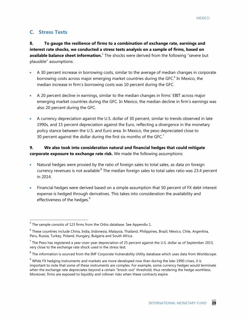
C. Stress Tests
8. To gauge the resilience of firms to a combination of exchange rate, earnings and
interest rate shocks, we conducted a stress tests analysis on a sample of firms, based on
available balance sheet information.5 The shocks were derived from the following “severe but
plausible” assumptions:
A 30 percent increase in borrowing costs, similar to the average of median changes in corporate
borrowing costs across major emerging market countries during the GFC.6 In Mexico, the
median increase in firm’s borrowing costs was 10 percent during the GFC.
A 20 percent decline in earnings, similar to the median changes in firms’ EBIT across major
emerging market countries during the GFC. In Mexico, the median decline in firm’s earnings was
also 20 percent during the GFC.
A currency depreciation against the U.S. dollar of 30 percent, similar to trends observed in late
1990s, and 15 percent depreciation against the Euro, reflecting a divergence in the monetary
policy stance between the U.S. and Euro area. In Mexico, the peso depreciated close to
30 percent against the dollar during the first six months of the GFC.7
9. We also took into consideration natural and financial hedges that could mitigate
corporate exposure to exchange rate risk. We made the following assumptions:
Natural hedges were proxied by the ratio of foreign sales to total sales, as data on foreign
currency revenues is not available.8 The median foreign sales to total sales ratio was 23.4 percent
in 2014.
Financial hedges were derived based on a simple assumption that 50 percent of FX debt interest
expense is hedged through derivatives. This takes into consideration the availability and
effectiveness of the hedges.9
5 The sample consists of 123 firms from the Orbis database. See Appendix 1.
6 These countries include China, India, Indonesia, Malaysia, Thailand, Philippines, Brazil, Mexico, Chile, Argentina,
Peru, Russia, Turkey, Poland, Hungary, Bulgaria and South Africa.
7 The Peso has registered a year-over-year depreciation of 25 percent against the U.S. dollar as of September 2015,
very close to the exchange rate shock used in the stress test.
8 The information is sourced from the IMF Corporate Vulnerability Utility database which uses data from Worldscope.
9 While FX hedging instruments and markets are more developed now than during the late-1990 crises, it is
important to note that some of these instruments are complex. For example, some currency hedges would terminate
when the exchange rate depreciates beyond a certain “knock-out” threshold, thus rendering the hedge worthless.
Moreover, firms are exposed to liquidity and rollover risks when these contracts expire.
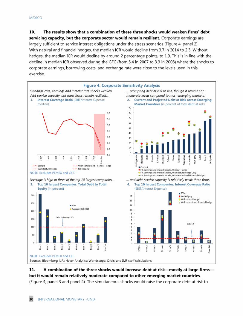
MEXICO
30 INTERNATIONAL MONETARY FUND
10. The results show that a combination of these three shocks would weaken firms’ debt
servicing capacity, but the corporate sector would remain resilient. Corporate earnings are
largely sufficient to service interest obligations under the stress scenarios (Figure 4, panel 2).
With natural and financial hedges, the median ICR would decline from 3.7 in 2014 to 2.3. Without
hedges, the median ICR would decline by around 2 percentage points, to 1.9. This is in line with the
decline in median ICR observed during the GFC (from 5.4 in 2007 to 3.3 in 2008) where the shocks to
corporate earnings, borrowing costs, and exchange rate were close to the levels used in this
exercise.
Figure 4. Corporate Sensitivity Analysis
Exchange rate, earnings and interest rate shocks weaken
debt service capacity, but most firms remain resilient…
… prompting debt at risk to rise, though it remains at
moderate levels compared to most emerging markets.
1. Interest Coverage Ratio (EBIT/Interest Expense,
median)
NOTE: Excludes PEMEX and CFE.
2. Current and Projected Debt at Risk across Emerging
Market Countries (in percent of total debt at risk)
Leverage is high in three of the top 10 largest companies… … and debt-service capacity is relatively weak three firms.
3. Top 10 largest Companies: Total Debt to Total
Equity (in percent)
NOTE: Excludes PEMEX and CFE.
4. Top 10 largest Companies: Interest Coverage Ratio
(EBIT/Interest Expense)
Sources: Bloomberg, L.P.; Haver Analytics; Worldscope; Orbis; and IMF staff calculations.
11. A combination of the three shocks would increase debt at risk—mostly at large firms—
but it would remain relatively moderate compared to other emerging market countries
(Figure 4, panel 3 and panel 4). The simultaneous shocks would raise the corporate debt at risk to
1.5
2.0
2.5
3.0
3.5
4.0
4.5
5.0
Scen
ario
s
2014
2013
2012
2011
2010
2009
2008
2007
Sample With Natural and Financial Hedge
With Natural Hedge No hedging
0
10
20
30
40
50
60
70
80
90
Phili
pp
ines
Ma
lays
ia
Ch
ile
Ru
ssia
S.A
fric
a
Th
ail
an
d
Pola
nd
Ch
ina
Mex
ico
Arg
enti
na
Ind
on
esia
Hu
nga
ry
Ind
ia
Bra
zil
Bu
lga
ria
CurrentFX, Earnings and Interest Shocks, Without HedgeFX, Earnings and Interest Shocks, With Natural Hedge OnlyFX, Earnings and Interest Shocks, With Natural and Financial Hedge
0
50
100
150
200
250
300
Firm
1
Firm
2
Firm
3
Firm
4
Firm
5
Firm
6
Firm
7
Firm
8
Firm
9
Firm
10
2014
Average 2010-2014
Debt to Equity = 100
14
19
24
America Movil
CEMEX Fomento Grupo Mexico
Wal-Mart
Coca-Cola
Grupo Televisa
Grupo Modelo
Grupo Elektra
2014No hedgingWith natural hedgeWith natural and financial hedge
-
1
2
3
4
5
6
7
8
9
10
Fir
m 1
Fir
m 2
Fir
m 3
Fir
m 4
Fir
m 5
Fir
m 6
Fir
m 7
Fir
m 8
Fir
m 9
Fir
m 1
0
ICR=1.5

MEXICO
INTERNATIONAL MONETARY FUND 31
38–40 percent of total debt (5.2–5.4 percent of GDP), from 27 percent of total debt (3.7 percent of
GDP) in 2014 (Box 1).
Box 1. Interest Coverage Ratio and Debt at Risk
Interest Coverage Ratio
A firm’s capacity to service debt hinges on its interest coverage ratio (ICR), computed as Earnings/Interest
Expense, where Earnings is measured by earnings before interest and taxation (EBIT)1. The lower the ratio,
the more the company is burdened by debt expense relative to earnings. An ICR of less than 1 implies that
the firm is not generating sufficient revenues to service its debt without making adjustments, such as
reducing operating costs, drawing down its cash reserves, or borrowing more. This analysis uses EBIT as a
measure of earnings instead of EBITDA (earnings before interest, taxation, depreciation and amortization) to
account for the need to replace assets and reinvest to ensure going-concern.
Debt at Risk
By the time a firm’s ICR dips below 1, it may already be in distress. As an early warning signal of potential
corporate difficulties ahead, analysts often use an ICR of 1.5 as a threshold. An ICR of below 1.5 also flags
potential vulnerability to funding risks, particularly when market liquidity thins in turbulent times. During the
Asian Financial Crisis, countries whose corporate sector with median ICR below 1.5 were more vulnerable.2
Accordingly, we define debt at risk as the debts of firms with ICR below 1.5. The debt at risk for each country
is computed as:
The share of debt at risk shows how much of these outstanding debts are vulnerable due to the weak debt
servicing capacity. A relatively high share of debt at risk shows that the country may be more susceptible to
corporate distress from macroeconomic and financial shocks.
Caveat
It is worth noting that the coverage and representativeness of the sample obtained from the Orbis database
vary across countries, and therefore sample selection bias can be a problem.
1. Also known as operating profit/loss
2. The median interest coverage ratio in Korea, Thailand and Indonesia were below 1.5.
12. Some of the largest firms have high leverage and low interest coverage. Among the top
ten largest companies (by asset size), four of them had total debt to total equity ratios above
100 percent, and three of them had ICRs below 1.5 in 2014 (Figure 4, panel 5 and panel 6). Our
stress tests analysis shows that a fourth firm would see its ICR decline below 1.5, bringing the

MEXICO
32 INTERNATIONAL MONETARY FUND
number of firms with ICR below 1.5 to four. The total debt of these four firms is around 3 percent of
GDP.
D. Impact on the Banking Sector
Figure 5. Impact on the Banking Sector
Higher corporate default will increase banks’
nonperforming loans…
...but banks have adequate loss absorbing buffers to
withstand the shocks.
1. Gross Nonperforming Loan Ratios (in percent of total
loans)
2. Loss Absorbing Buffer
1/ (in percent of risk-weighted assets)
1.Consist of Tier 1 capital and excess of loan loss reserves against the
current stock of nonperforming loans, normalized by risk-weighted assets.
Sources: Bankscope; Haver Analytics; and IMF staff calculations.
13. Commercial lending comprise a large share of total bank loans, but banks have
adequate buffers to absorb shocks in the corporate sector. Lending to nonfinancial corporations
account for half of total bank loans. Total gross nonperforming loans (NPL) in the banking sector
reached around 3 percent of total loans in 2014, slightly higher in larger banks compared to smaller
banks.10
Loss absorbing buffers comprising Tier 1 capital and excess of provisioning over NPLs are
strong, at 15 percent of risk-weighted assets. Our stress tests analysis, which assumes a default
probability of 15 percent for corporate debts with ICR below 1.5, suggests that the gross NPL ratio
could increase by 1.5 percentage points to 4.5 percent in a scenario where the corporate NPLs are
fully written-off (figure 5). In this scenario, the ratio of banks’ loss absorbing buffers to risk-weighted
assets would decline from 15 percent to 13.7 percent, still above Basel III’s minimum Tier 1 capital
ratio requirement of 8.5 percent.11
It is worth noting that commercial banks may be exposed to
funding risks in the stress scenario due to potential large deposit withdrawals, particularly from
corporations that are facing weaker financial positions.
10
These include NPLs from households and the corporate sector.
11 This includes capital conservation buffer of 2.5 percent.
2.0
2.5
3.0
3.5
4.0
4.5
5.0
With Recovery No Recovery (Full Write-Off)
Current Gross NPL ratioAfter Shocks on Corporate Sector with Natural and Financial HedgeAfter Shocks on Corporate Sector with Natural HedgeAfter Shocks on Corporate Sector with No Hedge
13.6
13.8
14.0
14.2
14.4
14.6
14.8
15.0
With Recovery No Recovery (Full Write-Off)
Current Buffer
After Shock on Corporate Sector with Natural and Financial Hedge
After Shock on Corporate Sector with Natural Hedge
After Shock on Corporate Sector with No Hedge

MEXICO
INTERNATIONAL MONETARY FUND 33
E. Impact on the Real Economy
14. While stress tests reveal that corporate balance sheets appear strong enough to
withstand large shocks, there could still be an impact on the real economy. The stress scenarios
discussed in the previous section reveal that widespread bankruptcies as a result of the assumed
shocks are unlikely. However, the median firm can still decide to retrench investment to rebuild
buffers if faced with shocks. Furthermore, firms outside the sample—if financially weaker—could still
default and may trigger higher NPLs at banks, which in turn, can curtail credit supply.
15. The median firm could lower investment up to 1.2 percentage points of the capital
stock in the most severe stress scenario. To derive the implications of the shocks for leverage, we
assume that total debt increases by the valuation loss on the proportion of debt denominated in
foreign currency due to the currency depreciation. Using estimates from Li, Magud, and Valencia
(2015)—relating investment rates to net leverage—the resulting increase in leverage would lead to a
reduction in investment rates between 0.3 and 1.2 percentage points of the capital stock. These
authors report an elasticity of real GDP growth to investment rates—measured in percent of a firms’
capital stock—of about 0.1. This elasticity implies that the reduction in investment rates could lead
to lower real GDP growth in 0.03 to 0.12 percent.
Stress Scenarios and Impact on Corporate Investment Rates
Stress Scenarios Increase in Net
Leverage
(Percentage points)
Reduction in Investment rates
(Percentage points)
High coefficient: 1/
-0.064
Low coefficient: 1/
-0.042
Scenario 1 (With natural hedges) 7.7 -0.49 -0.32
Scenario 2 (With natural and
financial hedges)
7.8 -0.50 -0.33
Scenario 3 (Without hedges) 18.8 -1.20 -0.79
Source: IMF staff calculation.
1/ Li, Magud, and Valencia (2015), coefficients estimated in a panel of 11,000 firms from 38 emerging markets,
including Mexico, relating investment rates—defined as capital expenditure divided by the capital stock—to net
leverage, defined as total debt minus cash stocks divided by total equity.
16. Additional real effects from lower supply of bank credit could arise if weaker firms
default. Firms in the above analysis are relatively large corporations with access to international
financial markets. Lacking firm-level data for the whole corporate sector, we assume—rather
conservatively—that firms outside the sample default with a 15 percent probability. This default rate
corresponds to Moody’s historical estimate for firms with ICR’s below 1.5. We extrapolate this
default rate to the whole portfolio of bank loans to the corporate sector. The resulting increase in
NPL’s is treated as a bank capital shock.12
Additional real effects could then arise from a reduction in
12
The increase in NPL’s would affect capital in the same period only to the extent that they exceed loss loan reserves.
However, even if loan loss reserves are enough to cover the increase in NPL’s, banks may wish to rebuild buffers.

MEXICO
34 INTERNATIONAL MONETARY FUND
the supply of bank credit in response to this capital shock. To estimate this effect we ran simple
regressions relating bank lending growth to the equity-to-assets ratio, which as the table below
shows, gives an estimated coefficient of around 2, similar to estimates for U.S. banks.13
17. Higher NPL’s at banks could reduce growth by up to 0.3 percent through a reduction
in the supply of credit. Empirical studies find elasticities of real GDP growth to bank credit growth
ranging from 0 to about 0.4, so a 1 percent reduction in credit growth leads to 0–0.4 percentage
points decline in real GDP growth.14
In times of severe recessions, the elasticity tends to be closer to
the upper limit, whereas during normal times it tends to be closer to zero. The elasticity depends
also on the degree of credit deepening. Given Mexico’s low credit deepening and the absence of a
deep recession, the elasticity would tend to be low; therefore, we assume a value of 0.15. The
estimated response of bank lending to the assumed shocks (between 1.4 and 1.7 percent) would
reduce growth between 0.2 and 0.3, depending on the stress scenario.
Stress Bank Lending Response to Bank Capital Shocks
Dependent variable: Loan growth
Loan growth
Loan growth
Loan growth
Size 0.017 0.024 -0.008 -0.058 (0.090) (0.140) (0.072) (0.125) Equity/Assets 2.041 1.888 (0.207)*** (0.261)*** Lagged Equity/Assets 0.927 0.990 (0.164)*** (0.146)*** Currency depreciation -0.189 -0.570 (0.480) (0.436) Inflation 3.719 -4.180 (12.578) (9.337) Time fixed effects No Yes No Yes Sample 2001-2014 2001-2014 2001-2014 2001-2014 Constant -44.640 -54.930 28.297 46.849 (132.419) (111.969) (102.250) (110.868) R
2 0.43 0.48 0.18 0.26
N 280 280 242 242 Source: IMF staff calculation.
Note: Fixed effects regressions with robust standard errors in parenthesis. Size denotes
the lagged value of the natural logarithm of total assets; Equity/Assets denotes total
equity divided by lagged total assets; currency depreciation measures the percentage
change in the exchange rate of the Mexican Peso vis-a-vis the U.S. Dollar; Inflation
denotes the percentage change in the CPI. * p<0.1; ** p<0.05; *** p<0.01
13
Hancock and Wilcox (1993, 1994), Bernanke and Lown (1991), Berger and Udell (1994), and Peek and Rosengren
(1994), Berrospide and Edge (2010) conducted studies with U.S. data and found coefficients ranging from 0.7 to 2.8,
in a variety of specifications.
14 Estimates vary depending on whether the regressions focus on normal times or periods of financial distress. For
instance, Driscoll (2004) finds no statistically significant effects, while Calomiris and Mason (2003) who study the real
effects of credit supply shocks around the Great Depression find an elasticity of 0.4.

MEXICO
INTERNATIONAL MONETARY FUND 35
18. Altogether, the assumed shocks could reduce growth by 0.2–0.4 percent, but in
combination with other shocks could lead to larger effects. The total effect reflects the impact of
the assumed shocks exclusively through a financial channel, operating both through lower
investment by firms in the sample in response to increased leverage and lower supply of bank
credit—from impaired loans to firms outside the sample. However, if the assumed shocks happen in
conjunction with other shocks—for instance, a negative growth surprise in the U.S.—the effects
could be much larger.
Impact of Higher NPLs on Credit Supply
Stress Scenarios Change in Bank Capital
(Percentage points)
Reduction in Loan Growth
(Percentage points)
High coefficient: 1/
2.041
Low coefficient: 1/
1.888
Scenario 1 0.74 -1.51 -1.40
Scenario 2 0.76 -1.55 -1.43
Scenario 3 0.84 -1.72 -1.59
Source: IMF staff calculation.
Note: scenarios treat the increase in NPLs as a bank capital shock.
1/ Coefficients correspond to those on the Equity/Assets ratio shown in Table 2.
F. Summary and Conclusion
19. While corporate credit metrics have weakened somewhat as of 2014, particularly
among large firms, the corporate sector remains resilient and bank sector buffers are strong.
The stress test analysis suggests that most firms have adequate capacity to service debt in a scenario
which combines a 30-percent exchange rate depreciation against the dollar, 30-percent increase in
borrowing costs, and 20-percent decline in earnings. Under these circumstances, banks’ buffers
remain strong and are sufficient to withstand the shocks in the corporate sector.
20. Notwithstanding the resilience of the corporate and banking sectors, the shocks could
still affect the real economy through lower investment and bank credit supply. Faced with
these shocks, firms could retrench investments to rebuild buffers. Weaker firms may default, thus
triggering higher NPLs, which could lead to a reduction in bank credit supply. Corporate data
disclosure requirements have been strengthened, but data issues still present a challenge for
monitoring risks.

MEXICO
36 INTERNATIONAL MONETARY FUND
Appendix I. Methodology for Corporate Sensitivity Analysis
A. Analytical Approach
A firm’s capacity to service debt hinges on its interest coverage ratio (ICR), computed as
EBIT/Interest Expense, where EBIT is earnings before interest and taxation1. The lower the ratio, the
greater the debt payment burden of the company. An ICR of less than 1 implies that the firm is not
generating sufficient revenues to service its debt without making adjustments, such as reducing
operating costs, drawing down its cash reserves, or borrowing more. This analysis uses an ICR
threshold of 1.5, which is a benchmark used widely by analysts as an early warning signal. Firms with
ICR below 1 may already be in distress.
B. Data Source
The analysis is based on annual firm-level balance sheet information from Orbis. This database has
123 Mexican firms with good data points, covering US$678 billion of assets (52 percent of GDP) and
US$359 billion of debt (28 percent of GDP). It includes public and private, large and small
companies.
C. Estimating Corporate Debt
As the breakdown of firm-by-firm foreign currency borrowing is not available through Orbis and
other in-house databases, FX debt is estimated at the aggregate level, by external debt statistics and
other sources as follows:
Sources of Corporate Borrowing Data
External Debt 1/ Quarterly External Debt Statistics (QEDS)
(http://web.worldbank.org/WBSITE/EXTERNAL/DATASTATISTICS/EXTD
ECQEDS/0,,contentMDK:20721958~menuPK:4704607~pagePK:641684
45~piPK:64168309~theSitePK:1805415,00.html)
NOTE: QEDS shows a breakdown of corporate external debt according
to debt from affiliates, direct investment and others which include
loans, money market instruments, trade credits, bonds and notes.
Domestic Banks Banking system data from “Financial Soundness Indicators”
Domestic Capital Markets Bloomberg
1/ While external debt could be in foreign or local currency, most foreign holdings of corporate debt are in hard
currencies.
Aggregate corporate debt is estimated as:
External Debt + Loans from Domestic Banks + Borrowings from Domestic Capital Markets
1 EBIT (also known as operating profit/loss) is used as a measure of earnings instead of EBITDA (earnings before
interest, taxation, depreciation and amortization) to account for the need for investment and replacement of assets.
MEXICO
INTERNATIONAL MONETARY FUND 37
D. Estimating Potential Exchange Rate Losses from Foreign Currency Debts
Potential exchange rate losses from foreign currency debt interest payment due in the current year
is estimated as:
The currency breakdown of external debt assumes that the share of EUR-denominated debt is
similar to the share of exports to the Euro area (18 percent) while the rest are denominated in US
dollar.
E. Accounting for Natural Hedges
FX losses from interest expense and revaluation of foreign currency debt principal and are offset by
FX gains from overseas earnings, computed as:
Assumptions underlying this estimation:
Foreign sales are assumed to be in foreign currencies.
The share of FX revenues is derived from the country trade weights.
The multiplication by EBIT (operating profit) effectively takes into account foreign currency costs,
as it assumes that the share of these costs are in proportion to foreign currency income.
It is worth noting that the effectiveness of natural hedges is an approximation as it may fall short of
expectations. Past episodes have demonstrated that overseas revenues could decline in tandem with
the depreciating currencies during turbulent periods.
F. Accounting for Financial Hedges
Currency hedging of foreign currency debts could also mitigate potential FX losses. Offset from
financial hedging of foreign currency debt principal and interest is computed as:
Hedge Ratio x FX losses from foreign currency debt interest
As information on financial hedging is sparse, this analysis assumes that at least 50 percent of
foreign currency debts are hedged, on aggregate basis.

MEXICO
38 INTERNATIONAL MONETARY FUND
G. Projecting the Increase in Nonperforming Loans
The increase in corporate nonperforming loans is projected from the after-shock corporate debt at
risk as follows:
Increase Corporate NPL = Increase in Corporate Loan at Risk x Probability of Default x Loss Given
Default
Increase in Corporate Loans at Risk: This is derived from extrapolating the risk of default of firms
with ICR’s below 1.5 to the entire portfolio of bank loans to the corporate sector. The implicit
assumption is that non-listed firms are financially weaker than listed firms.
Probability of default: This is assumed to be 15 percent based on Moody’s default probability for
corporate debts with interest coverage ratio of 1.5 over a three-year horizon(based on data from
1970-2012).
Loss Given Default: This is computed as an average of 45 percent (Basel II Foundation Approach
for senior claims on corporates, sovereigns and banks not secured by recognized collateral2) and
country-specific LGDs from The World Bank’s data on “Resolving Insolvency”3 (Appendix 1).
The ability of banks to withstand losses will depend on their loss absorbing buffers, which comprise
Tier 1 capital and the excess of provisioning over the stock of NPL. The after-shock loss absorbing
buffers can be computed as:
Tier 1 capital + Loan Loss Reserves – Existing Stock of NPL – Projected Increase in NPL
Risk-Weighted Assets
2 See section 287-288 of Basel II Accord ( http://www.bis.org/publ/bcbs128.pdf)
3 See http://www.doingbusiness.org/data/exploretopics/resolving-insolvency

MEXICO
INTERNATIONAL MONETARY FUND 39
References
Bank for International Settlements, 2015, “When the financial becomes real,” 85th
Annual Report,
1 April 2014–31 March 2015,” Basel.
Basel Committee on Banking Supervision, 2006, “International Convergence of Capital Measurement
and Capital Standards,” Basel: Bank for International Settlements, pp. 67-68.
Berger, A., and G. Udell, 1994. “Did Risk-based Capital Allocate Bank Credit and Cause a Credit
Crunch in the United States?" Journal of Money, Credit, and Banking 26, 585-628.
Bernanke, B., and C. Lown, 1991. “The Credit Crunch." Brookings Papers on Economic Activity 2, 205-
247.
Berrospide J. and M.E. Rochelle, 2010. “The Effects of Bank Capital on Lending: What do We Know,
and What Does it Mean?” Federal Reserve Board, Finance and Economics Discussion Series 2010-44.
Calomiris, C. W. and J.R. Mason, 2003, “Consequences of Bank Distress during the Great Depression,”
American Economic Review 93(3), pp. 937-47.
Chui, Michael et al., 2014, “Risks Related To EME Corporate Balance Sheets: The Role Of Leverage
And Currency Mismatch.” BIS Quarterly Review, September 2014,” Basel: Bank for International
Settlements, pp 35-47.
Claessens, Stijn et al., 2000, “Corporate Performance In The East Asian Financial Crisis.” The World
Bank Research Observer vol.15, no.1, Washington D.C.: The World Bank, pp 23-46.
Driscoll, J. C., 2004, “Does Bank Lending Affect Output? Evidence from the U.S. States,” Journal of
Monetary Economics 51(3), pp. 451-71.
Habermeier, Karl, Annamaria Kokenyne, and Chikako Baba, 2011, “The Effectiveness of Capital
Controls and Prudential Policies in Managing Large Inflows,” IMF Staff Discussion Note, SDN/11/14,
Washington D.C.: International Monetary Fund.
Hancock, D., and J. Wilcox, 1993. “Has There Been a Capital Crunch in Banking? The Effects on Bank
Lending of Real Estate Market Conditions and Bank Capital Shortfalls." Journal of Housing
Economics 3, 31-50.
Hancock, D., and J. Wilcox, 1994. “Bank Capital and Credit Crunch: The Roles of Risk-Weighted and
Unweighted Capital Regulations." Journal of the American Real Estate and Urban Economics
Association 22, 59-94.
International Monetary Fund, December 2014, “Staff Guidance Note on Macroprudential Policy—
Detailed Guidance on Instruments,” Washington D.C.

MEXICO
40 INTERNATIONAL MONETARY FUND
Kraft, Evan and Tomislav Galac, 2011, “Macroprudential Regulation of Credit Booms and Busts-The
Case of Croatia”, World Bank Policy Research Working Paper, No. 5572, Washington D.C.: The World
Bank.
Li, Delong, Nicolás Magud, and Fabián Valencia, 2015, “Financial Shocks and Corporate Investment
in Emerging Markets: Ability vs. Willingness,” forthcoming IMF working paper.
Singh, Manmohan, 2007, “Use of Participatory Notes in Indian Equity Markets and Recent Regulatory
Changes,” IMF Working Paper, WP/07/291, Washington D.C.: International Monetary Fund.
Peek, J., and E. Rosengren, 1994. “Bank Real Estate Lending and the New England Capital Crunch”
Journal of the American Real Estate and Urban Economics Association 22, No. 1, pp. 33-58.

MEXICO
INTERNATIONAL MONETARY FUND 41
A CARBON TAX PROPOSAL FOR MEXICO1
Mexico has set clear commitments to reduce carbon emissions ahead of the 2015 Paris summit on
climate change. A recent reform—pending Senate approval––proposed fixing excises on gasoline and
diesel—in lieu of the current system of variable excises—and to allow the domestic price of these fuels
to move more closely in line with international prices until they are fully liberalized in 2018. Taking
into account climate change, air pollution, and traffic-related negative externalities associated with
fossil fuel combustion, this paper finds that the proposed level of excises are close to optimal. However,
natural gas and coal would remain significantly under taxed, if taxation is to become the main tool to
correct for negative climate change externalities. Setting carbon taxes at optimal levels in Mexico could
reduce carbon emissions by 6 percent over the medium term, contributing non-trivially to the goal of
reducing carbon emissions in 25 percent by 2030.
A. Introduction
1. Fossil fuels are a critical energy input in industrial production and in final
consumption, but their combustion has also harmful environmental and public health
impacts. These consequences can have potentially sizable costs to the economy. However, energy
prices in many countries are often set at levels that do not reflect these costs or are even subsidized.
Given the seriousness of the environmental and public health problems associated with fossil fuel
combustion, addressing them with targeted policy instruments is critical.
2. Mexico has been at the forefront among emerging markets in setting clear
commitments to address these concerns. Mexico enacted in 2012 a climate change law which
aimed at creating a legal framework to ensure the implementation of policies aiming at protecting
the environment. It also created the Climate Change National Institute in charge of measuring
carbon emissions. In 2013, Mexico released the national strategy for climate change, outlining clear
commitments to reduce carbon emissions. In the same year, Mexico introduced a carbon tax on all
fossil fuels as part of a broader fiscal reform. Recently, Mexico reiterated its commitments to reduce
carbon emissions ahead of the Paris summit on climate change to take place in late 2015.
3. Fiscal instruments targeted directly at the sources of environmental harm help address
these concerns but also generate fiscal revenues. As long as these revenues avoid increasing
other taxes that distort economic activity, environmental protection is achieved at the lowest overall
cost to the economy.
1 Prepared by Fabian Valencia. The author thanks Dora Iakova, Luis Madrazo, Carlos Muñoz, Ian Parry, Glenn Sheriff,
and seminar participants at the Mexican Ministry of Finance and the Central Bank of Mexico for insightful comments
and suggestions and Alexander Herman for outstanding research assistance. This paper used Parry and others (2014)
comprehensive calculations of optimal carbon taxes and updates it to 2015 prices.

MEXICO
42 INTERNATIONAL MONETARY FUND
B. Mexico’s Current Excise Taxes on Fossil Fuels
4. Most fossil fuels in Mexico are subject to excise taxes, including a carbon component.
A carbon tax refers to a tax directly linked to the level of carbon dioxide (CO2) emissions. The tax is
often expressed per ton of CO2 and varies across fossil fuels depending on the amount of emissions
they produce when burned. The carbon component of fuel excises in Mexico was introduced as part
of the 2013 tax reform, as a special tax on production and services (IEPS) which came to effect in
2014. It covers all fossil fuels-except natural gas and crude oil (IEPS law, art. 8), and Jet fuel2—with
rates varying depending on the carbon content. A second component of fuel excises in Mexico is
earmarked for states and local governments (IEPS law, art. 2o-A II), and affects only gasoline (regular
and premium) and diesel. A third component is a variable excise which also affects only gasoline and
diesel. It is a residual between an international reference price converted to local currency and the
regulated retail price.3 Since the international reference price co-moves one-for-one with
international oil prices, the variable excise component moves countercyclically with the international
price of oil, leading to higher fiscal revenues when international oil prices fall.
Fuel Price Structure and Gasoline Prices
Sources: Secretary of Energy; and IMF staff calculations.
5. As of 2014, fossil fuel excise taxes in Mexico implied the lowest taxation rate among
OECD countries. Implicit carbon taxes, defined as all excise taxes on fossil fuels, were low in Mexico,
in particular as the variable excise mechanism implied a subsidy on fossil fuels until late 2014.
2 Natural gas was exempted on account of being the cleanest fossil fuel. A 2013 Presidential Decree exempted Jet
fuel from the carbon tax in adherence to international agreements signed by Mexico, which included the exemption
of this fossil fuel from taxes.
3 The regulated retail price includes the carbon tax, excises earmarked for states, VAT, transport costs, distribution
margins, and technical losses due to evaporation.
-4
-2
0
2
4
6
8
10
12
14
16
18
Jan-Aug
2014
Jan-Aug
2015
Jan-Aug
2014
Jan-Aug
2015
Jan-Aug
2014
Jan-Aug
2015
Jan-Aug
2014
Jan-Aug
2015
Jan-Aug
2014
Jan-Aug
2015
Regular Gasoline Premium Gasoline Diesel Fuel Oil Jet Fuel
Excises earmarked for States
Carbon tax
Variable excises
Other components
a) Fuel Price Structure (Current pesos per liter)
8
9
10
11
12
13
14
Jan
-14
Feb
-14
Mar-
14
Ap
r-14
May-1
4
Jun
-14
Jul-
14
Au
g-1
4
Sep
-14
Oct-
14
No
v-1
4
Dec-1
4
Jan
-15
Feb
-15
Mar-
15
Ap
r-15
May-1
5
Jun
-15
Jul-
15
Au
g-1
5
Retail price
International price + excises and other components
b) Domestic Retail Price of Regular Gasoline(Current pesos per liter)

MEXICO
INTERNATIONAL MONETARY FUND 43
Implicit Carbon Tax Rates
Sources: EIA; and OECD.
Note: Mexico as of 2014, all others as of 2013.
6. The collapse of oil prices since late 2014 turned the variable excise tax positive.
Domestic retail prices of gasoline and diesel continued to be adjusted upwards as oil prices
declined, although at a much slower pace in 2015 than in the previous year. Therefore; Mexico no
longer subsidizes diesel and gasoline given current domestic and international fuel prices. However,
if the current variable excise mechanism were to be kept, the variable excise tax could turn into a
subsidy again if international fuel prices rise.
C. In Search for a New Energy Taxation Mechanism
7. A recent reform—pending Senate approval—proposed a mechanism of excise taxes to
ensure fuel subsidies are eliminated permanently and smooth the transition to fully
liberalized domestic fuel prices. Mexico plans to liberalize domestic fuel prices by 2018, which
implies a necessity to replace the current system of excises with a new mechanism. Ideally, this new
mechanism should ensure a proper taxation of fossil fuels to reflect environmental and public health
costs. The 2016 budget proposed a replacement of the variable component of the excise tax at
levels near those observed this year with a fixed excise system. As of the writing of this paper, the
proposal had been approved by the lower chamber of Congress. To smooth the transition toward
fully liberalized domestic fuel prices, the Ministry of Finance would define a price band during this
transition period (2016–2017) that would allow domestic fuel prices to fluctuate more in line with
international prices.
8. A fixed excise tax on fossil fuels—equivalent to a carbon tax—is also a viable option to
tackle the national climate change strategy goals, which have been reinforced with the recently
announced commitments ahead of the 2015 Paris summit on climate change. Mexico has pledged
to reduce carbon emissions in 30 percent by 2020, and 25 percent by 2030, relative to baseline
projections. A carbon tax is administratively simple since Mexico has already a system in place. Since
a carbon tax raises the price of each ton of carbon emitted into the atmosphere, it raises the cost of
emissions. Higher costs induce a market response throughout the entire economy, creating
incentives for fuel users to shift to alternative ways of production and ultimately lower carbon
0
20
40
60
80
100
120
140
160
CH
ELU
XN
OR
NLD
DN
KSW
EIR
LIS
LIT
AIS
RG
BR
SV
NG
RC
FR
AFIN
DEU
AU
TESP
PRT
BEL
TU
RJP
NH
UN
SV
KC
ZE
NZ
LKO
REST
PO
LA
US
CH
LC
AN
USA
MEX
(U.S. dollars per ton of CO2)

MEXICO
44 INTERNATIONAL MONETARY FUND
emissions. While Mexico’s contributions to carbon emissions are still small globally, they have been
rising faster than the OECD average over the last decade.
Carbon Dioxide Emissions
Source: OECD.
9. From a fiscal perspective, fixing excise taxes on fuels at an optimal level could help
stabilize tax revenues without relying on other, more distortionary taxation. Carbon taxes
allow the extraction of a double dividend. Not only do they help correct an important negative
externality but they also allow raising fiscal revenues without relying on taxes that tend to distort
economic activity. If the variable excise system were maintained, lower tax revenues as international
oil prices recover could lead to pressures to make up the shortfall by raising revenues through
distortionary taxation. Setting excise taxes at optimal levels can also lead to lower public spending
on health in the long-term if lower combustion of fossil fuel leads to a lower incidence of pollution-
related diseases, keeping everything else equal.4
D. Estimating Optimal Carbon Tax Rates on Fossil Fuels for Mexico5
10. The methodology considers three main categories of externalities associated with
fossil fuel combustion: climate change, air pollution, and those related to traffic. It relies on
country-specific data wherever available and applicable to estimate the social cost of fossil fuel
consumption in an attempt to estimate an optimal Pigouvian tax. While for some externalities
variation in country-specific factors such as level of income, population density, and traffic
congestion lead to different optimal taxes, this is not the case for climate change. For climate
change the associated damage from carbon emissions is the same regardless of the fuel combustion
4 Parry and all (2014) calculate a potential reduction in deaths due to air pollution-related diseases of up to
20 percent for the case of Mexico.
5 This section briefly summarizes the methodology followed in Parry and all (2014) to compute Mexico’s suggested
carbon tax rates. Further details and data sources can be found in Parry and all (2014) while theoretical
underpinnings of fuel taxation can be found in Parry and Small (2005) and more general issues on optimal
environmental taxation in the presence of other taxes in Bovenberg and Goulder (1996).
0
1,000
2,000
3,000
4,000
5,000
6,000
7,000
8,000
9,000
0
100
200
300
400
500
600
700
1980 1984 1988 1992 1996 2000 2004 2008 2012
Mexico Argentina
Brazil Venezuela
Turkey OECD average
United States (RHS) China (RHS)
(Million metric tons)

MEXICO
INTERNATIONAL MONETARY FUND 45
process or where emissions are released. The methodology then assumes a uniform cost across
countries, per unit of carbon emissions. More specifically, each externality is dealt with as follows:
Climate change is assumed to lead to a monetary cost of US$ 38 per metric ton of CO2. The
assumed cost is within the range of estimates provided by the US Interagency Working Group
on the Social Cost of Carbon (2013 update), obtained from simulations of a range of models,
under different discount rate assumptions.6 These estimates, however, vary widely. As an
illustration, the average estimated cost for 2015 ranges from US$12 per metric ton of CO2, if the
discount factor is set to 5 percent, to US$38 and US$58 per metric ton of CO2 if the discount
factor is lowered to 3 and 2.5 percent respectively. This assumption, together with data on
carbon content of fossil fuels, allows deriving carbon charges for all fossil fuels that would reflect
the cost of climate-change externalities.
Tax Rate Due to Climate Change
Sources: Parry et al. (2014); and IMF staff calculations
To estimate the cost of air pollution, the approach uses empirical information on the link
between exposure and incidence of pollution-related diseases. Local air pollution can lead to
a wide array of harmful environmental consequences. However, to focus on those that are most
severe, the analysis centers on premature human mortality. The methodology first determines
how much polluted air is inhaled by exposed population. Relying on existing empirical evidence,
it then assesses how this pollution exposure affects mortality risks, accounting for factors, such
as the age and health of the population, which determine the vulnerability of the exposed
population to pollution-related illness. The next step is the monetization of health effects. This
6 Quantifying climate change costs is subject to a great deal of uncertainty due in principal to three features of
climate change. The first is the highly uncertain effect of emissions on specific climate outcomes; the second is the
unknown form of human adaptation to problems building up over decades and centuries; and the third is the
differences of opinion about the appropriate analytical procedure for aggregating effects occurring over long time
intervals.
0.0
0.5
1.0
1.5
2.0
2.5
3.0
3.5
4.0
Coal Natural gas Gasoline Diesel
(U.S. dollars per GJ)
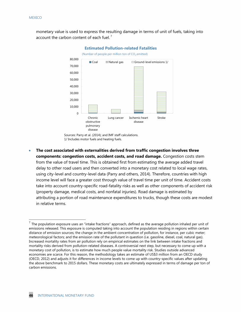
MEXICO
46 INTERNATIONAL MONETARY FUND
monetary value is used to express the resulting damage in terms of unit of fuels, taking into
account the carbon content of each fuel. 7
Estimated Pollution-related Fatalities
Sources: Parry et al. (2014); and IMF staff calculations.
1/ Includes motor fuels and heating fuels.
The cost associated with externalities derived from traffic congestion involves three
components: congestion costs, accident costs, and road damage. Congestion costs stem
from the value of travel time. This is obtained first from estimating the average added travel
delay to other road users and then converted into a monetary cost related to local wage rates,
using city-level and country-level data (Parry and others, 2014). Therefore, countries with high
income level will face a greater cost through value of travel time per unit of time. Accident costs
take into account country-specific road-fatality risks as well as other components of accident risk
(property damage, medical costs, and nonfatal injuries). Road damage is estimated by
attributing a portion of road maintenance expenditures to trucks, though these costs are modest
in relative terms.
7 The population exposure uses an “intake fractions” approach, defined as the average pollution inhaled per unit of
emissions released. This exposure is computed taking into account the population residing in regions within certain
distance of emission sources; the change in the ambient concentration of pollution, for instance, per cubic meter;
meteorological factors; and the emission rate of the pollutant in question (i.e. gasoline, diesel, coal, natural gas).
Increased mortality rates from air pollution rely on empirical estimates on the link between intake fractions and
mortality risks derived from pollution-related diseases. A controversial next step, but necessary to come up with a
monetary cost of pollution, is to estimate how much people value mortality risk. Studies outside advanced
economies are scarce. For this reason, the methodology takes an estimate of US$3 million from an OECD study
(OECD, 2012) and adjusts it for differences in income levels to come up with country-specific values after updating
the above benchmark to 2015 dollars. These monetary costs are ultimately expressed in terms of damage per ton of
carbon emissions.
0
10,000
20,000
30,000
40,000
50,000
60,000
70,000
80,000
Chronic
obstructive
pulmonary
disease
Lung cancer Ischemic heart
disease
Stroke
Coal Natural gas Ground-level emissions 1/
(Number of people per million ton of CO2 emitted)

MEXICO
INTERNATIONAL MONETARY FUND 47
Components of Corrective Tax Rate due to Traffic-related Externalities
Source: Parry et al. (2014).
11. Estimates of an optimal carbon tax for Mexico reach, quoted in MEX$ per GJ, 18 for
natural gas, 77 for regular gasoline, 97 for diesel, and 36 for coal.8 Local air pollution and traffic-
related are the dominant externalities for gasoline and diesel. Natural gas, being a much cleaner
fossil fuel, requires only a small tax to correct for air pollution externalities from its combustion, but
it still requires a significant tax to correct for climate change externalities as its combustion releases
significant carbon dioxide into the atmosphere. Coal, on the other hand, requires a higher tax than
natural gas on account of both, air pollution and climate change externalities.
8 The estimates are computed in current US dollars, converted to MEX$ using purchasing power parity exchange
rates, as recommended by Parry and others (2014). Purchasing power parity exchange rates take into account the
local price level and thus reflect more accurately than market exchange rates people’s ability to purchase goods or
pay out of their own income for risk reductions.
0.0
0.2
0.4
0.6
0.8
1.0
1.2
1.4
Au
stra
lia
Au
stri
aB
elg
ium
Can
ad
aC
hile
Cze
ch R
ep
ub
lic
Den
mark
Est
on
iaFin
lan
dFra
nce
Germ
an
yG
reece
Hu
ng
ary
Icela
nd
Irela
nd
Isra
el
Italy
Jap
an
Ko
rea
Luxe
mb
ou
rgM
exi
coN
eth
erl
an
ds
New
Zeala
nd
No
rway
Po
lan
dPo
rtu
gal
Slo
vak R
ep
ub
lic
Slo
ven
iaSp
ain
Sw
ed
en
Sw
itze
rlan
dTu
rkey
Un
ited
Kin
gd
om
Un
ited
Sta
tes
Accidents Congestion
a) Gasoline(U.S. dollars per liter)
0.0
0.2
0.4
0.6
0.8
1.0
1.2
1.4
Au
stra
lia
Au
stri
aB
elg
ium
Can
ad
aC
hile
Cze
ch R
ep
ub
lic
Den
mark
Est
on
iaFin
lan
dFra
nce
Germ
an
yG
reece
Hu
ng
ary
Icela
nd
Irela
nd
Isra
el
Italy
Jap
an
Ko
rea
Luxe
mb
ou
rgM
exi
coN
eth
erl
an
ds
New
Zeala
nd
No
rway
Po
lan
dPo
rtu
gal
Slo
vak R
ep
ub
lic
Slo
ven
iaSp
ain
Sw
ed
en
Sw
itze
rlan
dTu
rkey
Un
ited
Kin
gd
om
Un
ited
Sta
tes
Congestion Accidents Road damage
b) Diesel(U.S. dollars per liter)
Estimated Optimal Carbon Taxes for Mexico
Sources: Parry et al. (2014); and IMF staff calculations.
0
20
40
60
80
100
120
140Climate change
Local air pollution
Traffic-related
(Pesos per GJ, 2015)
Natural gas Regular
Gasoline
Diesel Coal

MEXICO
48 INTERNATIONAL MONETARY FUND
12. Estimated tax rates are likely to be underestimated and should be interpreted as a
lower bound. Models with richer micro-foundations, taking into account the interaction of carbon
taxes with labor income taxes, can lead to higher carbon tax rates (Parry and Small, 2005). In the
specific case of regular gasoline in Mexico, these interactions can lead to a carbon tax 35-percent
higher than the one shown above (Anton-Sarabia and Hernandez-Trillo, 2014). Moreover, the
methodology employed in this paper considers only premature human mortality when assessing the
consequences of air pollution. However, there are other non-fatal consequences that can also have
important economic costs. For instance, there is empirical evidence suggesting that increased
pollution reduces labor supply (Hanna and Oliva, 2015); it lowers labor productivity (Graff and Nidel,
2012); and it affects children’s learning (Sanders, 2012).
13. Proposed excise tax levels are close to optimal. In an attempt to correct for some of the
underestimation of optimal tax levels by the baseline methodology, the estimated taxes are scaled
up by 35 percent—roughly the estimated contribution of interactions with labor income taxes
discussed above. For simplicity, it is assumed that the scaling factor is the same for diesel and
gasoline. The resulting “adjusted” Pigouvian tax is shown in the next figure together with the
proposed taxes in the 2016 budget—in the case of gasoline and diesel—and those currently in place
for coal and natural gas.9 The methodology employed here offers no specific tax for premium
gasoline, but its higher energy content would suggest lower taxes than regular gasoline. Natural gas
and coal are significantly under taxed—if their externalities were to be addressed entirely through
taxation—but the proposed levels for gasoline and diesel are close to optimal. Note that the
assumed adjustment to the estimated Pigouvian tax still has unaccounted factors, such as the
impact of pollution on labor productivity and supply, which implies that the adjusted tax should still
be seen as a lower bound.
Estimated Optimal Carbon Taxes in Mexico
Sources: Parry et al. (2014); and IMF staff calculations.
9 The 2016 budget proposed a reform to the IEPS law which encompasses substituting the variable excise component
for gasoline and diesel with a fixed excise equal to the level shown in the graph. The proposed reform does not affect
other fossil fuels, with natural gas continuing to be exempted.
0
20
40
60
80
100
120
140
Natural Gas Coal Diesel Regular
gasoline
Premium
gasoline
Current/2016 Budget
Adjusted Optimal
(Pesos per GJ, 2015)
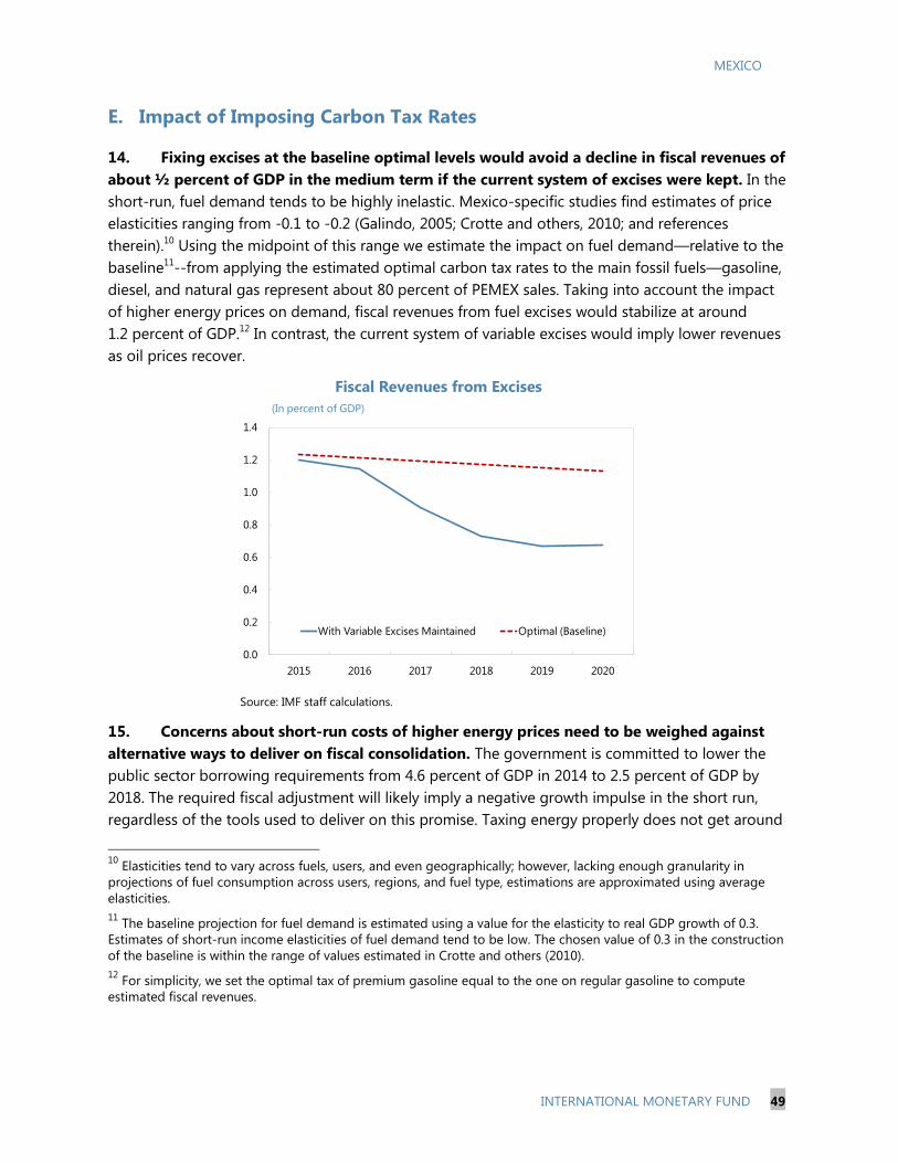
MEXICO
INTERNATIONAL MONETARY FUND 49
E. Impact of Imposing Carbon Tax Rates
14. Fixing excises at the baseline optimal levels would avoid a decline in fiscal revenues of
about ½ percent of GDP in the medium term if the current system of excises were kept. In the
short-run, fuel demand tends to be highly inelastic. Mexico-specific studies find estimates of price
elasticities ranging from -0.1 to -0.2 (Galindo, 2005; Crotte and others, 2010; and references
therein).10
Using the midpoint of this range we estimate the impact on fuel demand—relative to the
baseline11
--from applying the estimated optimal carbon tax rates to the main fossil fuels—gasoline,
diesel, and natural gas represent about 80 percent of PEMEX sales. Taking into account the impact
of higher energy prices on demand, fiscal revenues from fuel excises would stabilize at around
1.2 percent of GDP.12
In contrast, the current system of variable excises would imply lower revenues
as oil prices recover.
Fiscal Revenues from Excises
Source: IMF staff calculations.
15. Concerns about short-run costs of higher energy prices need to be weighed against
alternative ways to deliver on fiscal consolidation. The government is committed to lower the
public sector borrowing requirements from 4.6 percent of GDP in 2014 to 2.5 percent of GDP by
2018. The required fiscal adjustment will likely imply a negative growth impulse in the short run,
regardless of the tools used to deliver on this promise. Taxing energy properly does not get around
10
Elasticities tend to vary across fuels, users, and even geographically; however, lacking enough granularity in
projections of fuel consumption across users, regions, and fuel type, estimations are approximated using average
elasticities.
11 The baseline projection for fuel demand is estimated using a value for the elasticity to real GDP growth of 0.3.
Estimates of short-run income elasticities of fuel demand tend to be low. The chosen value of 0.3 in the construction
of the baseline is within the range of values estimated in Crotte and others (2010).
12 For simplicity, we set the optimal tax of premium gasoline equal to the one on regular gasoline to compute
estimated fiscal revenues.
0.0
0.2
0.4
0.6
0.8
1.0
1.2
1.4
2015 2016 2017 2018 2019 2020
With Variable Excises Maintained Optimal (Baseline)
(In percent of GDP)

MEXICO
50 INTERNATIONAL MONETARY FUND
this implication but it helps achieve this goal without having to rely on other, more distortionary
taxation, such as income tax. Furthermore, it creates incentives to move toward cleaner and cheaper
sources of energy with positive long-term implications on growth and health.
16. Over the long-run, the suggested taxation can contribute to a reduction of about 6
percent in carbon emissions, relative to our baseline. Mexican-specific studies find long-run price
elasticities for fuel demand ranging from below -0.5 to numbers close to -1 (Galindo, 2005; Crotte
and others, 2010 and references therein), depending on different econometric methods, geographic
level, and time periods. Estimates at the national level fall closer to the -0.5 estimate than to -1. We
use then -0.5—also used in Parry and others (2014)—in our calculations to derive long-term
implications on carbon emissions. Under this approach, taxation alone can contribute non-trivially to
the recent pledge of reducing carbon emissions in 25 percent by 2030.
F. Conclusions
17. The proposed reform to fix excise taxes on gasoline and diesel to eliminate fuel
subsidies permanently is a welcome development. The proposed reform—already approved by
the lower chamber of Congress but pending Senate approval—would replace the current system of
variable excises with a more conventional fixed excise per liter of gasoline and diesel. The reform is
an important step in the process of liberalization of domestic fuel prices and developing a true
domestic energy market. It also eliminates permanently inefficient fuel subsidies, which were in
place until 2014, and avoid a decline in fiscal revenues under the current system once oil prices
recover.
18. From an environmental perspective, the proposed excise levels are close to an optimal
Pigouvian tax, and could reduce carbon emissions by 6 percent. This reduction in carbon
emissions would contribute non-trivially to Mexico’s reiterated commitments ahead of the Paris
summit on climate change to take place in late 2015. Needless to say, the estimates are subject to
substantial amount of uncertainty and will need to be updated frequently as technology and
empirical evidence evolve.

MEXICO
INTERNATIONAL MONETARY FUND 51
References
Anton-Sarabia, Arturo and Fausto Hernandez-Trillo, 2014. “Optimal Gasoline Tax in Developing, Oil-
producing Countries: The Case of Mexico.” Energy Policy, vol. 67, pages 567-571.
Bovenberg, A. Lans and Goulder, Lawrence H., 1996. “Optimal Environmental Taxation in the
Presence of Other Taxes: General-Equilibrium Analyses.” American Economic Review, 1996, 86(4), pp.
985–1000.
Crotte, Amado, Robert Noland, and Daniel Graham, 2010. “An Analysis of Gasoline Demand
Elasticities at the National and Local Levels in Mexico.” Energy Policy, vol. 38, pages 4445-4456.
Hanna, Rema and Paulina Oliva, 2015. “The Effect of Pollution on Labor Supply: Evidence from a
Natural Experiment in Mexico City.” Journal of Public Economics, vol. 122, pages 68-79.
Galindo, Luis, 2005. “Short- and long-run demand for energy in Mexico: a cointegration approach.”
Energy Policy, vol. 33, pages 1179-1185.
Graff, Joshua and Matthey Neidell, 2012. “The impact of pollution on worker productivity.” American
Economic Review, vol. 102, pages 3652-3673.
Parry, Ian, Dirk Heine, Eliza Lis, and Shanjun Li, 2014. “Getting Energy Prices Right.” International
Monetary Fund, Washington D.C.
Parry, Ian and Kenneth A. Small, 2005. “Does Britain or the United States Have the Right Gasoline
Tax? American Economic Review, vol. 95, No. 4, pages 1276-1289.
Sanders, Nicholas, 2012. “What doesn't kill you makes you weaker: prenatal pollution exposure and
educational outcomes.” Journal of human resources, vol. 47, pages 826-851.
US Interagency Working Group on the Social Cost of Carbon, 2013. “Thechnical Update of the Social
Cost of Carbon for Regulatory Impact Analysis-Under Executive Order 12866.” United States
Government.

MEXICO
52 INTERNATIONAL MONETARY FUND
STRENGTHENING MEXICO’S FISCAL FRAMEWORK1
Mexico’s fiscal framework has improved significantly in recent years, but some shortcomings remain.
This chapter argues that the addition of a nominal anchor, limiting discretion under exceptional
circumstances, and a fiscal council can enhance the framework’s role as commitment device to fiscal
discipline and reduce medium-term fiscal policy uncertainty, particularly after a large negative shock.
A new nominal anchor can take the form of an explicit permanent ceiling on the public sector
borrowing requirements (PSBR). Setting such ceiling at most at 2.5 percent of GDP would ensure that
public debt remains at prudent levels with high probability. Limiting discretion under the exceptional
circumstances clause can be achieved by tightening the triggers to invoke it, capping the allowed
deterioration in the PSBR, and adding explicit rules about how to return fiscal policy to equilibrium
once the clause is invoked. Introducing a fiscal council could help maintain fiscal discipline by
providing a non-partisan evaluation of fiscal policy and raising public awareness of the importance of
a sound fiscal position.
A. Introduction
1. Macroeconomic management in Mexico has improved significantly since the nineties,
allowing Mexico to confront the global financial crisis in 2009 with strong fiscal buffers.
Unsound banking practices combined with external imbalances, and public debt heavily skewed
towards short-term maturities and foreign-currency denomination culminated in the mid-90’s with
the Tequila crisis. Since then much has changed. On the fiscal front in particular, the years before the
global financial crisis were characterized by declining public deficits, prudent public debt levels and
composition—largely long-term and domestic-currency denominated—and a new fiscal framework
aiming at locking in these gains.
2. These fiscal buffers allowed Mexico to act counter-cyclically in 2009, but the crisis left
a legacy of high public deficits. The crisis hit Mexico hard, but Mexico’s strong fiscal buffers
allowed the country to inject a fiscal stimulus to mitigate the real effects of the shock. However,
persistently high fiscal deficits since the crisis suggest that the fiscal framework was effective in
allowing flexibility to respond to the global shock but it did not ensure a gradual but steady return
to low fiscal deficits in the aftermath of the crisis.
1 Prepared by Fabian Valencia. The author thanks Carlos Caceres, Dora Iakova, Alex Klemm, Luis Madrazo, Robert
Rennhack, and seminar participants at the Bank of Mexico and the Ministry of Finance for valuable comments and
suggestions and Alexander Herman for outstanding research assistance.

MEXICO
INTERNATIONAL MONETARY FUND 53
B. Mexico’s Fiscal Framework: Recent Improvements and Pending Tasks
3. Important aspects of the fiscal framework have improved in recent years, including the
addition of new fiscal targets and the creation of a sovereign wealth Fund. The fiscal
responsibility law, enacted in 2006, aimed at locking in the low fiscal deficits that characterized fiscal
performance prior to the crisis. It did so by introducing a zero-balance target on the traditional
measure of the deficit. However, the traditional fiscal balance did not reflect properly public debt
dynamics (Box 1). As a result, the 2014 amendments to the fiscal responsibility law added the PSBR
as a target, a much more comprehensive measure of the public deficit, and introduced a cap on the
real growth of current structural spending to limit procyclicality in a framework with a headline
deficit target. In addition, the amendments changed the way oil revenues are managed. Starting in
2015, a new sovereign wealth fund, the Mexican Oil Fund, manages all hydrocarbon-related wealth,
which should help better insulate public spending from transitory fluctuations in oil revenues.
Sources: IMF World Economic Outlook; National authorities; and IMF staff
calculations.
Notes: LA-6 excluding Mexico is comprised of Brazil, Chile, Colombia, Peru,
and Uruguay. EM comparator group is comprised of India, Indonesia, Poland,
Russia, Thailand, and Turkey.
-2
-1
0
1
2
3
4
5
6
7
1997 1999 2001 2003 2005 2007 2009 2011 2013
Mexico
LA-6 (excl. Mexico)
EM group simple average
Overall Public Sector Deficit(In percent of GDP)
MEX Average
2001-08
MEX Average
2009-14
MEX Average
1997-2000

MEXICO
54 INTERNATIONAL MONETARY FUND
Box 1. The Fiscal Responsibility Law: Main Features
The 2006 fiscal responsibility law (FRL) aimed at locking in low deficits and providing a
framework for smoothing the spending of oil revenues over the commodity cycle. Over 2004-
2006, Mexico maintained fiscal deficits—measured by the traditional balance—close to zero. The FRL
aimed at locking in this performance by introducing a zero-balance target on the traditional fiscal deficit
measure. It also introduced a reference oil price to be used for revenue projections to smooth the
impact of short-term fluctuations in oil prices in the budget. Excess oil revenues were to be used in part
to compensate for certain budgetary overruns (e.g., higher interest costs, and the higher fuel bill of the
state electricity company) and in part saved into several stabilization funds (to be used in case of
shortfalls), but only up to certain limits.
The framework also increased accountability and transparency of fiscal policy. The law called for
annual budgets to be presented in the context of a long-term quantitative framework, with projections
for the next five years, and mandated an assessment of the fiscal costs associated with new legal
initiatives. Other provisions to strengthen expenditure management included greater transparency and
controls over the use of trust funds, greater accountability in the selection of investment projects and
social programs through cost-benefit analyses, and steps toward performance-based budgeting,
requiring the establishment of indicators to measure program outcomes.
The original target, however, had shortcomings. It was too narrow to conduct an appropriate
assessment of the fiscal stance and to reflect properly public debt dynamics. Moreover, the target was
later relaxed to exclude PEMEX capital investment and more recently to exclude also investment by the
state-owned electricity company, CFE, and some strategic projects.
The fiscal framework did not insulate fully public spending from temporary oil-price fluctuations.
In principle, the intention of the framework was to save temporary oil windfalls and smooth policy over
the oil price cycle. In practice, only a small fraction of the oil revenue windfall was saved (IMF 2013).
The 2014 amendments added new fiscal targets. They include the PSBR, a more comprehensive
measure of the fiscal deficit and thus more relevant for debt dynamics, and a cap on the real rate of
growth of structural current spending, set initially at 2 percent and equal to potential output growth
from 2017 on. The amendments also introduced targets for PEMEX and CFE, consistent with their new
legal status.
A Mexican Oil Fund was also created to manage hydrocarbons-related revenues. The fund now
manages all oil-related revenues and payments (except for taxes). The Federal Government no longer
receives oil-revenues directly from PEMEX, except for income taxes, also applicable to private oil
companies, and instead receives transfers from the Mexican Oil Fund for up to 4.7 percent of GDP. Once
long-term savings in the Mexican Oil Fund reach 3 percent of GDP, part of the additional inflows will be
spent. The previous budgetary revenue stabilization fund (FEIP) and the states revenue stabilization fund
(FEIEF) will continue to operate and will be the first line of defense in case of temporary and unexpected
declines in revenues. Long-term savings in the Mexican Oil Fund can be used to cover temporary, but
persistent declines in revenues only after the FEIP and FEIEF have been exhausted.

MEXICO
INTERNATIONAL MONETARY FUND 55
4. But the framework still needs an adequate nominal anchor while limited discretion
under exceptional circumstances could reduce fiscal policy uncertainty in the aftermath of a
large shock. One shortcoming is rooted in how much discretion the framework allows once a shock
hits, through the exceptional circumstances clause, both in terms of when and how much the fiscal
stance can deteriorate and how it should be brought back to equilibrium. Once in equilibrium, a
nominal anchor guiding fiscal policy in normal times would help strengthen the role of the
framework as a commitment device to fiscal discipline. In the original framework, the permanent
zero-balance target on the traditional measure of the deficit meant to serve as a nominal anchor.
However, its effectiveness was eroded by revisions to its definition and the narrowness of its scope.
C. Dealing with Exceptional Circumstances
5. The case for countercyclical fiscal policy is stronger when large shocks—like the global
financial crisis—hit the economy. Art. 17 of the FRL allows for ex ante deviations from the
traditional balance target under exceptional circumstances. But ideally, only large shocks should
trigger the exceptional circumstances clause. The main rationale is that only in those circumstances
one can be certain that a large negative output gap has opened up. Countercyclical fiscal policy can
therefore help, provided there is policy space. Under small shocks, the need for counter cyclical fiscal
policy is weaker due to the inherent uncertainty surrounding estimates of potential output and
downward rigidities in spending, which may make it difficult to reverse increases in expenditure.
6. Tighter triggers to allow invoking the exceptional circumstances clause would ensure
fiscal policy discretion is only used when it is strictly necessary. The FRL’s regulation includes
specific triggers for the exceptional circumstances clause. However, some of these triggers can be
reached even under mild shocks.2 The triggers could be adjusted so that the clause is triggered, for
instance, only after a 1–2 standard-deviation temporary shock. In some countries, there are no
numerical triggers, but invoking exceptional circumstances is constrained by requiring approval by a
supermajority in Congress (Switzerland) or severe economic downturns (European Union’s fiscal
compact).
7. Once exceptional circumstances are justified, the fiscal framework would also benefit
from tighter rules on guiding the return of fiscal policy to equilibrium. This could include
limiting the fiscal deterioration allowed in the case of a large shock. For example, in Panama and
Peru, the exceptional circumstances clause allows relaxing the deficit ceiling temporarily from
1 percent of GDP up to 3 percent of GDP and 2.5 percent of GDP, in each respective country (Budina
and others, 2012). Complementing the framework also with well-specified rules of how to return to
equilibrium would ensure a gradual but steady reduction in the PSBR in the aftermath of a large
shock. There are several options to achieve this goal. In the case of Peru, the fiscal framework
2 Examples of triggers include a decline in tax revenues for 2.5 percent in real terms and a 10-percent decline in oil
prices, both representing only slightly less than half a standard deviation shock (computed on the annual changes in
both variables over 1996-2014).

MEXICO
56 INTERNATIONAL MONETARY FUND
requires an improvement of at least 0.5 percent of GDP per year until the deficit falls below the
1 percent target. Germany and Switzerland have so called “debt brakes,” which involve recording
deviations from the deficit ceiling in a notional account until the cumulative balance crosses a
predetermined threshold. When this threshold is crossed, the balance needs to be brought down to
zero within three annual budgets (Switzerland) or when the economy is recovering (Germany).3
D. A New Nominal Anchor
8. Outside exceptional times, a permanent ceiling on the PSBR could serve as a natural
new nominal anchor. Current legislation does not specify a particular ceiling for the PSBR but
instead requires that a target for the current year and the medium-term is specified in the budget
documents. Current medium-term fiscal targets include reducing the PSBR to 2.5 percent of GDP by
2018 and maintaining it at that level at least until 2021 (the last year of the current projection).
9. The implication of alternative ceilings on the PSBR on the probability distribution of
public debt is explored through stochastic simulations. Lacking consensus in the literature on a
debt threshold beyond which growth prospects are hurt (IMF, 2012), current debt levels are used as
benchmark. Mexico’s public debt-to-GDP ratio is projected to rise slightly above 50 percent but
under the baseline scenario, public debt would fall back to 50 percent by 2020. This level of public
debt is also within the range of debt ceilings introduced by several countries into legislation (Box 2).
The simulations also assume that the PSBR ceiling can be relaxed up to 2 percentage points of
GDP—when real GDP growth is one standard deviation below the mean—but it is brought down to
below the ceiling within 3 years. These assumptions help derive implications for public debt not only
from imposing a permanent ceiling as proposed but also from limiting the use of the exceptional
circumstances clause.
10. A permanent ceiling of 2.5 percent of GDP would keep public debt below 50 percent
with high probability in the baseline scenario. 4 The simulations are initialized in 2018. Two
scenarios are considered, a baseline scenario in which potential GDP growth stays at 3.3 percent
over the long term—corresponding to staff’s medium-term potential growth projections—and one
in which it is only 2.5 percent, roughly the average growth over the last two decades. Under the
baseline scenario, a ceiling of 2.5 percent of GDP would keep public debt below 50 percent with
3 In Germany, only those deviations that did not result from errors in real GDP growth projections enter the notional
account, whereas in Switzerland all misses count.
4 Public expenditures are assumed to remain constant as a fraction of GDP at 2018 levels, except when the deficit
ceiling binds, in which case expenditures are adjusted as needed to meet the PSBR ceiling. The GDP deflator is
assumed to grow 3 percent per year, the permanent inflation target of the Bank of Mexico. Fiscal revenues and real
GDP growth are treated as stochastic variables. To this end, a linear regression model is estimated relating fiscal
revenues growth in real terms to its lagged value and real GDP growth. Similarly, an ARMA (1, 1) model is estimated
with real GDP growth data where the constant term is adjusted so that the unconditional mean of real GDP growth
equals 3.3 percent under the baseline scenario or 2.5 percent under the low growth scenario. Random draws are
obtained from the empirical distribution of the error term in both empirical models to construct 500 paths of
25 years each for the stochastic variables.

MEXICO
INTERNATIONAL MONETARY FUND 57
82 percent probability over the next 25 years. Setting the ceiling at 2 percent or 1.5 percent of GDP
would increase this probability to 95 percent and 97 percent respectively. These probabilities
correspond to the whole path of the public debt-to-GDP ratio remaining below 50 percent of GDP.
The median debt path shows an average debt level—after 25 years—of about 44 percent of GDP,
39 percent of GDP, and 32 percent of GDP, depending on whether the PSBR ceiling is set at 2.5, 2, or
1.5 percent of GDP, respectively.
Box 2. Examples of Fiscal Rules with Explicit Debt Ceilings
European Union: In 2012, 25 members of the European Council signed the Fiscal Compact
agreeing to adopt in legislation national rules that limit annual structural deficits to a maximum of
0.5 percent of GDP and a commitment to continuously reduce the public-debt-to GDP ratio to the
60 percent of GDP threshold, among other elements.
Panama: The Fiscal social Responsibility Law limits the deficit of the nonfinancial public sector at
1 percent of GDP and a debt ceiling of 40 percent of GDP to be reached by 2017.
Indonesia: The State Finance Law and Government Regulation limits the consolidated national
and local government budget deficit to 3 percent of GDP and public debt to 60 percent of GDP.
Hungary: The Constitution establishes a debt limit of 50 percent of GDP and public debt must be
reduced until this debt ceiling is achieved except when real GDP contracts.
Preemptive Action Triggers
Debt thresholds trigger actions before the debt reaches the ceiling to minimize the risk of
breaching it. Examples include Poland and Slovakia, both with debt rules setting a debt ceiling of
60 percent of GDP. In Slovakia, when debt reaches 50 percent of GDP, the Minister of Finance is
required to explain to parliament and suggest corrective measures. At 53 percent of GDP, a
package of measures is to be passed and wages are frozen. At 55 percent, automatic expenditure
cuts for 3 percent and an expenditure freeze for the subsequent year come into effect. At
57 percent of GDP, a balanced budget is required.
11. Under pessimistic potential growth assumptions, only a ceiling of at most 2 percent of
GDP would ensure public debt remains below 50 percent with high probability. Under the low
potential growth scenario, a PSBR ceiling of 2.5 percent of GDP would imply a 60 percent probability
of public debt remaining below 50 percent of GDP over the 25-year simulation period. However, a
ceiling of 2 percent or tighter would keep public debt below 50 percent of GDP with 90 percent
probability or higher. For this low growth scenario, the median debt path shows an average debt
level—after 25 years—of about 48 percent of GDP, 42 percent of GDP, and 36 percent of GDP,
depending on whether the PSBR ceiling is set at 2.5, 2, or 1.5 percent of GDP, respectively.

MEXICO
58 INTERNATIONAL MONETARY FUND
Figure 1. Probability Distribution of Public Debt Under Different PSBR Ceilings
Sources: National authorities; and IMF staff calculations.
Note: CDF= Cumulative Distribution Function. The simulation is implemented by first estimating empirical models on real GDP
growth and fiscal revenues, which are used to simulate 500 paths of 25 years each. The key underlying assumptions include
constant public expenditure in percent of GDP, and annual percent change of GDP deflator equal to 3 percent. The use of
exceptional circumstances clause is embedded by relaxing the ceiling in 2 percentage points when real GDP growth is 1 standard
deviation below the mean, but it is required to bring it back to below the permanent ceiling within three years. The plots show the
unconditional distribution of public debt and the median public debt path across all 500 simulations.

MEXICO
INTERNATIONAL MONETARY FUND 59
E. Fiscal Council
12. The introduction of a non-partisan fiscal council can help making the proposed
modifications to the fiscal framework more effective.5 There is a growing interest worldwide in
strengthening institutional frameworks through empowering independent watchdogs (Hagemann,
2011; OECD, 2013; IMF, 2013). Fiscal councils contribute to the policy debate by disseminating
analyses, opinions, recommendations, and forecasts. Once they have an established reputation, fiscal
councils’ opinions and recommendations can help improve fiscal performance. The general idea is
that enhanced transparency improves democratic accountability; raises public awareness about the
consequences of unsound policy actions; and increases the reputational and electoral costs of
reneging on fiscal commitments.
13. There is empirical evidence suggesting that fiscal councils contribute to improved
fiscal performance. Evidence from country-specific case studies (Belgium, Chile, Hungary, and
United Kingdom) looking at fiscal performance before and after the establishment of a fiscal council
suggests that fiscal councils contributed to improve fiscal performance (Hagemann, 2011; Lebrun,
2006; Coene, 2010). Cross-country evidence based on EU countries survey data also suggests fiscal
councils can improve fiscal performance in particular when a numerical fiscal rule is in place (Debrun
and Kumar, 2007). However, Debrun and Kinda (2014), using an econometric approach in a sample
of 58 advanced and emerging markets over 1990–2011, find that the mere existence of fiscal
councils is not by itself conducive to stronger fiscal balances. It depends on the characteristics of
fiscal councils. Those fiscal councils with either legal independence, adequate human resources, or in
charge of monitoring adherence to a numerical fiscal rule, assessment and/or production of
forecasts, costing government measures, and those with high media impact are often associated
with better fiscal outcomes. Debrun and Kinda (2014) also find that fiscal councils and their key
characteristics are associated with lower forecast errors on projections of fiscal outcomes.
14. A non-partisan fiscal council with an explicit mandate to assess the sustainability of
public finances could help enforce the proposed modifications to the fiscal framework. The
mandate of the fiscal council can be gradually broadened as the council establishes its reputation as
a non-partisan and unbiased institution (Box 3 provides examples of mandates). The council could
issue assessments and recommendations on the appropriate fiscal policy stance, on compliance with
the fiscal framework, and on the sustainability of public finances more broadly. Even if the
recommendations are not binding, they could force the fiscal authority to follow a comply-or-
explain approach. It could even provide inputs directly into the budget process, for instance by
being in charge of macroeconomic and fiscal revenue projections or calculating potential output.
5 Fiscal councils, broadly defined, refer to an independent public institution informing the public fiscal debate
without partisan influence. More specific definitions narrow down the functions of a fiscal council to comply with this
overarching objective and elaborate on what independence means. IMF (2005, p. 4) suggests that a council’s main
functions could include the provision of independent analysis on fiscal policy developments, the preparation of
unbiased projections, and the issuance of “normative judgments” (recommendations) on fiscal policy. OECD (2013)
clarifies that the notion of “independence” relates to the non-partisan nature of the council’s analysis, and that the
work of the council should be forward-looking in essence.

MEXICO
60 INTERNATIONAL MONETARY FUND
Box 3. Examples of Fiscal Council Mandates1
Some fiscal councils prepare budgetary forecasts ranging from projections that are mandatorily used
in the budget process to just a technical review of the budget assumptions. For instance, the Dutch
government uses the macroeconomic, revenue, and expenditure forecasts prepared by the fiscal council. In
the United Kingdom, the Office of Budget Responsibility (OBR) produces 5-year economic and fiscal
forecasts, with the Treasury subject to a “comply or explain” clause. In the United States, Canada, and
Denmark, the fiscal council’s forecasts only serve as a comparator to official projections. In some countries
(Colombia and Chile), the fiscal council is responsible to verify the calculation of potential output or the
estimation of the reference price of commodities such as oil and copper.
A number of councils produce also medium- to long-term fiscal projections. The US Congressional
Budget Office forecasts typically cover a 10 year period, while the British, Canadian, Korean, and Dutch
councils produce longer-term projections (over 40- to 75-year horizons) often in the context of a specific
mandate to analyze the sustainability of public finances.
Councils also conduct cost analyses of policy measures. These range from simple reviews of tax and
spending estimates used in the budget to an extensive costing of specific policy initiatives. The latter
approach is often seen in countries where the fiscal council is associated with the legislative branch (e.g.
Canada, Korea, and the United States). The Dutch fiscal council routinely responds to requests from line
ministries regarding new policy initiatives and provides cost-benefit analysis of major infrastructure projects.
In the United Kingdom, the OBR must review the tax and spending estimates produced by government
ministries as part of the draft budget proposal, but it does not cost specific policy initiatives. In Australia and
the Netherlands, assessments extend also to the economic and budgetary impact of political platforms prior
to elections.
Councils can carry out other functions including the analysis of efficiency of public expenditure and
fostering coordination among the various entities of the general government. In Korea and Slovenia,
the council makes recommendations for improving the efficiency and effectiveness of government programs
(existing or planned). Several councils have also an explicit mandate to examine fiscal issues related to state
and local governments and/or public enterprises (e.g. Portugal and Austria).
_________ 1 Further details can be found in IMF (2013).
F. Conclusions
15. The global financial crisis and its aftermath uncovered strengths and weaknesses in
Mexico’s fiscal framework. The fiscal framework was effective in allowing flexibility to respond to
the crisis and allowed Mexico to act countercyclically in response to the shock. However, it was not
very effective in ensuring a gradual but steady return to low fiscal deficits.
16. Going forward, a new nominal anchor, limited discretion under exceptional
circumstances, and a fiscal council, can make the fiscal framework more effective. A new
nominal anchor, such as an explicit permanent ceiling on the PSBR, could help enhance the fiscal
framework’s role as a commitment device to fiscal discipline. Limiting the use of the exceptional
circumstances clause to only large shocks; and limiting discretion under exceptional circumstances—
by capping the allowed deterioration in the PSBR and specifying explicitly in the framework the
adjustment path towards equilibrium—would also reduce fiscal policy uncertainty in the aftermath
of a large shock. Furthermore, a fiscal council could help enforce the proposed modifications to the
framework and strengthen fiscal discipline by providing assessments and recommendations on fiscal
policy.

MEXICO
INTERNATIONAL MONETARY FUND 61
References
Budina, Nina; Tidiane Kinda; Andrea Schaechter; and Anke Weber, 2012, “Fiscal Rules at a Glance:
Country Details from a New Dataset,” IMF Working Paper No. 12/273.
Coene, Luc, 2010. “Lessons from Belgium”, Paper presented at the Conference on Independent Fiscal
Institutions, Budapest, 18-19 March.
Debrun, Xavier and Tidiane Kinda, 2014. “Strengthening Post-Crisis Fiscal Credibility: Fiscal Councils
on the Rise—A New Dataset.” International Monetary Fund working paper No. 14/58.
Debrun, Xavier and Manmohan S. Kumar, 2007, “Fiscal Rules, Fiscal Councils and All That:
Commitment Devices, Signaling Tools or Smokescreens?” in: Banca d’Italia (eds.) Fiscal Policy:
Current Issues and Challenges, Papers presented at the Banca d’Italia workshop held in Perugia, 29–
31 March 2007, pp. 479–512.
Hagemann, Robert, 2011, “How Can Fiscal Councils Strengthen Fiscal Performance?” OECD Journal:
Economic Studies, Vol. 2011/1.
International Monetary Fund, 2005. “Promoting Fiscal Discipline: Is There a Role for Fiscal Agencies?”
IMF Policy Paper, (Washington, DC: International Monetary Fund).
International Monetary Fund, 2012, “The Good, the Bad, and the Ugly: 100 Years of Dealing with
Public Debt Overhangs,” World Economic Outlook, October 2012, chapter 3.
International Monetary Fund, 2013a. “Mexico—Reforms to the Fiscal Framework.” Mexico: Selected
Issues, International Monetary Fund country report No. 13/333.
International Monetary Fund, 2013b. “The Functions and Impact of Fiscal Councils.” IMF Policy paper,
(Washington, DC: International Monetary Fund).
Lebrun, Igor, 2006. “Fiscal Councils, Independent Forecasts, and the Budgetary Process: Lessons from
the Belgian Case.” In Ayuso-i-Casals and others, Policy Instruments for Sound Fiscal Policy, Palgrave-
MacMillan.
Organization for Economic Cooperation and Development, 2013, “OECD Principles for Independent
Fiscal Institutions,” Public Governance and Territorial Development Directorate, May.

MEXICO
62 INTERNATIONAL MONETARY FUND
THE EFFECTS OF FX INTERVENTION IN MEXICO1
FX Intervention in Mexico takes place through a rules-based approach. Over the last year there have
been three major changes to these rules. This background note estimates the effect on the Mexican
peso following these announcements. The results suggest that the March and the July 2015
announcements led to an appreciation of the peso by 3 and by 2 percent respectively, in their
immediate aftermath. The results on volatility are more mixed. While volatility does decline following
these announcements, the effect is not as robust as the one for the level.
A. Introduction
1. Mexico’s FX Intervention takes place through a rules-based approach. Pemex is
required to sell the foreign exchange from its export proceeds as well as from its net foreign
borrowing to the central bank, which in the absence of FX sales yields a steady accumulation of
reserves. The Foreign Exchange Comission (Comisión de Cambios), with members from the Ministry
of Finance and central bank, sets the rules for FX intervention.
2. The intervention rules are adjusted based on FX market conditions. There have been
four significant changes since 2011, with three taking place over the last year.2
On November 29, 2011, a rule was adopted providing 400 million dollars in FX auctions with a
minimum price equal to the previous day benchmark exchange rate plus 2 percent. Thus, actual
FX sales would only take place if the peso depreciated more than 2 percent. Since the minimum
price in these auctions was set at a fairly large threshold for a one-day depreciation, they were
only triggered on a few occasions. This rule remained in place until April 8, 2013.
On December 8, 2014, that mechanism was reintroduced but reducing the sale amount to 200
million dollars and the one-day depreciation threshold to 1.5 percent.
On March 11, 2015, daily FX auctions of 52 million dollars until June 8 were announced. These
auctions did not have a minimum price, so that was the actual amount of FX sold each day.
These sales roughly offset the reserve accumulation stemming from Pemex, in essence
amounting to a halt in reserve accumulation. On May 22, 2015, the daily FX auctions were
extended until end-September.
On July 30, 2015, the daily auctions were increased to 200 million dollars. The one-day
depreciation threshold for an additional 200 million dollar auction was reduced from 1.5 to
1 percent. On September 28, these measures were extended until November 30, 2015.
B. Peso Response in the Aftermath of Changes to FX Intervention Policy
3. The Mexican peso did not appreciate significantly in the aftermath of most
announcements, but did tend to outperform comparator currencies (Figure 1). This is
1 Prepared by Marcos Chamon.
2 We consider six announcements, two of which were extensions of a previously announced rule.

MEXICO
INTERNATIONAL MONETARY FUND 63
consistent with the change in rules contributing to a modest appreciation, but being adopted in the
midst of depreciation pressures (the usual challenge with assessing the effectiveness of FX
intervention). A similar comparison for the evolution of option-implied volatility suggests a more
mixed effect (Figure 2).
Figure 1: Evolution of the Exchange Rate vis-a-vis the U.S. Dollar
Around Foreign Exchange Intervention Program Announcement Dates 1/
Source: Bloomberg L.P.; and IMF staff calculations.
1/ An increase denotes a depreciation.
90
92
94
96
98
100
102
104
10/31/11 11/15/11 11/30/11 12/15/11
Brazil
Chile
Colombia
Peru
Mexico
November 29, 2011
(Index, Nov. 28, 2014=100)
85
90
95
100
105
110
2/9/15 2/24/15 3/11/15 3/26/15 4/10/15
BrazilChileColombiaPeruMexico
March 11, 2015
(Index, Mar. 10, 2015=100)
90
92
94
96
98
100
102
104
106
108
11/10/14 11/25/14 12/10/14 12/25/14
Brazil
Chile
Colombia
Peru
Mexico
December 8, 2014
(Index, Dec. 7, 2014=100)
92
94
96
98
100
102
104
106
108
7/10/15 7/25/15 8/9/15
Brazil
Chile
Colombia
Peru
Mexico
July 30, 2015
(Index, Jul. 29, 2015=100)
94
96
98
100
102
104
106
108
4/22/15 5/7/15 5/22/15 6/6/15
Brazil
Chile
Colombia
Peru
Mexico
May 22, 2015
(Index, May 21, 2015=100)
86
88
90
92
94
96
98
100
102
104
106
9/10/15 9/25/15 10/10/15
Brazil
Chile
Colombia
Peru
Mexico
September 28, 2015
(Index, Sep. 25, 2015=100)

MEXICO
64 INTERNATIONAL MONETARY FUND
Figure 2: Evolution of Option-Implied Exchange Rate Volatility Around
Foreign Exchange Intervention Program Announcement Dates
Source: Bloomberg L.P.; and IMF staff calculations.
60
70
80
90
100
110
120
10/31/11 11/15/11 11/30/11 12/15/11
Brazil
Chile
Colombia
Peru
Mexico
November 29, 2011
(Index, Nov. 28, 2014=100)
70
75
80
85
90
95
100
105
110
115
120
2/9/15 2/24/15 3/11/15 3/26/15 4/10/15
Brazil
Chile
Colombia
Peru
Mexico
March 11, 2015
(Index, Mar. 10, 2015=100)
60
70
80
90
100
110
120
130
140
150
11/10/14 11/25/14 12/10/14 12/25/14
Brazil
Chile
Colombia
Peru
Mexico
December 8, 2014
(Index, Dec. 7, 2014=100)
80
85
90
95
100
105
110
115
120
7/10/15 7/25/15 8/9/15
Brazil
Chile
Colombia
Peru
Mexico
July 30, 2015
(Index, Jul. 29, 2015=100)
90
95
100
105
110
115
120
4/22/15 5/7/15 5/22/15 6/6/15
Brazil
Chile
Colombia
Peru
Mexico
May 22, 2015
(Index, May 21, 2015=100)
70
75
80
85
90
95
100
105
110
9/10/15 9/25/15 10/10/15
Brazil
Chile
Colombia
Peru
Mexico
September 28, 2015
(Index, Sep. 27, 2015=100)

MEXICO
INTERNATIONAL MONETARY FUND 65
4. We estimate the impact of the announcements controlling for changes in global
financial conditions and comparator currencies. We run the following regression for the log
change in the exchange rate:
which includes as explanatory variables the log change in the exchange rates for Chile, Colombia,
and Peru, and an index of the value of the US dollar vis-à-vis other major currencies, the log change
in the VIX, oil prices, and the change in the US 10 year yield, as well as dummy variables that equal
to one on the day in which a change in intervention policy is announced.3 For example, the dummy
D1 is equal to one on November 29, 2011, and zero everywhere else. We also include the lagged
value of these dummies in the regression, which allows us to estimate the effect over a longer time
window.4 Our time sample starts in 2010, and we consider dummies for the six announcements in
Figure 1. All of the changes in FX intervention rules took effect on the day following their
announcement (except for the March 11th
, 2015 announcement which took effect on the same day
and the May 22nd
, 2015 extension to the daily FX auctions which took effect on June 9th
, 2015).
Focusing on their immediate aftermath provides a reasonable empirical strategy to quantify the
effect, provided these announcements were indeed the major financial news around those dates.
The exchange rate is a forward looking variable, and should adjust as the market prices in the
expected stream of future intervention. But our estimates may underestimate the full effect if
different frictions prevent that adjustment from taking place right away.
5. The regression points to a significant appreciation of the peso following the
November 2011, and the March and July 2015 announcements. The table below reports the
estimated effects for windows that range from only the day of the announcement (t) to windows
that include the five working days after the announcement (t to t+5). The cumulative appreciation by
t+5 was 2.5 and 3.4 percent following the November 2011 and March 2015 announcements,
respectively, while the effect from the July 2015 announcement peaks at a 2 percent appreciation at
t+2. The December 2014 announcement does not seem to affect the exchange rate. The May 2015
3 We did not include the Brazilian real in the list of explanatory variables. While historically the Mexican peso often
commoved with the Brazilian real, the latter has become more volatile in the recent period, being driven by
significant home-grown vulnerabilities, which could add noise to our estimation.
4 For example, the effect on the exchange rate on the day of that announcement is given by the coefficient 1,0,
whereas the cumulative effect including the following day is given by 1,0+ 1,1, and the cumulative effect over the
first 3 days is given by 1,0+ 1,1+ 1,2.
, , , ,
5 5 5 5 5 6
1, 1, 2, 2, 3, 3, 4, 4, 5, 5, 6, 6,
0 0 0 0 0
1 2 3
4 5
0
6 7
log log log log
log log log 10
MEX t CHL t COL t PER t
t t t t
t t t t t t
e e e e
DollarIndex VIX OIL US Y
D D D D D D
t

MEXICO
66 INTERNATIONAL MONETARY FUND
and September 2015 also have little or no effect, possibly because they involved extensions of an
existing rule, which were likely anticipated by the market.5
6. We cannot determine whether the estimated effects are permanent or transitory. The
standard deviation for daily changes in the peso is around 0.7 percent, while the standard deviation
from the residuals from this regression is about 0.5 percent (depending on the sample). Over time,
the standard error of the cumulative change increases with the square root of t. So estimates that
use a horizon beyond a few days will imply standard errors that are wide enough to overwhelm any
effect we could plausibly expect from these announcements.
Estimated Effect of the Different Announcements on the Level of the MXN/USD Exchange Rate 1/
Announcement
Nov 2011 Dec 2014 Mar 2015 May 2015 Jul 2015 Sep 2015
Cumulative Change on the Exchange Rate Since Announcement (Percent) 2/ t -1.28**
-0.76
-1.25**
-0.19
-0.71
-0.42
[0.52]
[0.52]
[0.52]
[0.52]
[0.52]
[0.52]
t to t+1 -1.64**
-0.56
-1.36*
-0.37 -1.54**
-0.51
[0.74]
[0.74]
[0.73]
[0.73]
[0.74]
[0.74]
t to t+2 -1.61*
-0.92
-1.48
-1.5* -1.96**
-0.66
[0.9]
[0.91]
[0.9]
[0.9] [0.91]
[0.9]
t to t+3 -1.55
-0.03
-1.89*
-1.51 -1.28
-0.02
[1.04]
[1.05]
[1.04]
[1.04]
[1.05]
[1.04]
t to t+4 -2.13*
-0.27
-2.18*
-1.39 -1.13
-0.21
[1.16]
[1.17]
[1.16]
[1.16] [1.17]
[1.16]
t to t+5 -2.53**
-0.42
-3.36***
-0.96 -1.7
0.62
[1.27] [1.29] [1.28] [1.28] [1.28] [1.28] Source: IMF staff calculations.
1/ Based on a regression of the log change in the Mexican peso exchange rate on the log change in the exchange
rate for Chile, Colombia, and Peru, the exchange rate of the dollar vis-à-vis a basket of major currencies, the VIX, oil
prices, the change in the U.S. treasury 10 year yield, and dummy variables for the different announcements and their
lags. For conciseness, only the cumulative effect implied by the dummies is reported. Standard errors in brackets. *,
**, and *** denote statistical significance at the 10, 5 and 1 percent level, respectively.
2/ An increase denotes a depreciation.
7. A similar regression points to more mixed effects on the option-implied volatility.
There is a decline in volatility, at least on impact, following the first three announcements. It initially
increases before declining in the aftermath of the July 2015 announcement. The results need to be
interpreted with caution, since intervention may increase volatility in the very short-term (e.g. as it
facilitates a correction) while potentially reducing it over a longer horizon (beyond what can be
5 It is worth noting that the impact on the exchange rate is not proportional to the size of the intervention implied by
the announcement. For example, the estimated response to the July 2015 announcement is smaller than the one for
the March 2015 announcement, even though the latter almost quadrupled the amount of daily FX sales from the
former. There are many factors that could contribute to a less than one-for-one response, including the possibility
that intervention becomes less effective as its size increases.

MEXICO
INTERNATIONAL MONETARY FUND 67
meaningfully captured by our regressions). More generally, volatility is often associated in the
empirical literature to the variance of the shocks, or as in our case, to the option-implied parameter
for the standard deviation of the exchange rate stochastic process. But in practice authorities are
more likely to be worried about sharp movements in the exchange rate. That risk may be better
captured by sizable deviations of the level from its perceived equilibrium rather than traditional
measures of volatility (which for the same reasons may be an imperfect measure of disorderly
market conditions).6
Estimated Effect of the Different Announcements on the Percent Change in the Option-
Implied Volatility of the MXN/USD Exchange Rate 1/
Announcement
Nov 2011 Dec 2014 Mar 2015 May 2015 Jul 2015 Sep 2015
Cumulative Change on the Option-Implied Volatility Since Announcement (Percent)
t -4.51*
-4.04*
-6.49***
-1.68
2.46
2.26
[2.39]
[2.39]
[2.39]
[2.39]
[2.39]
[2.39]
t to t+1 -2.99
-5.34
-4.7
0.02
1.97
2.59
[3.38]
[3.39]
[3.37]
[3.37]
[3.38]
[3.37]
t to t+2 -2.85
-5.45
-4.25
-4.64
-3.41
-1.78
[4.14]
[4.2]
[4.13]
[4.14]
[4.17]
[4.13]
t to t+3 -4.76
4.07
-6.91
-4.91
-8.05*
-3
[4.77]
[4.86]
[4.78]
[4.78]
[4.8]
[4.77]
t to t+4 -6.14
2.86
-6.5
-3.47
-7.97
-4.78
[5.34]
[5.43]
[5.35]
[5.34]
[5.37]
[5.34]
t to t+5 -7.37
10.59*
-1.56
-3.39
-9.76*
-4.11
[5.85] [5.93] [5.86] [5.85] [5.88] [5.85] Source: IMF staff calculations.
1/ Based on a regression of the log change in the option-implied volatility for the Mexican peso on the log change of
the option-implied exchange rate volatility for Chile, Colombia, and Peru, the exchange rate of the dollar vis-à-vis a
basket of major currencies, the VIX, oil prices, the change in the U.S. treasury 10 year yield, and dummy variables for
the different announcements and their lags. For conciseness, only the cumulative effect implied by the dummies is
reported. Standard errors in brackets. *, **, and *** denote statistical significance at the 10, 5 and 1 percent level,
respectively.
8. Signaling effects may have strengthened the effects of FX intervention. There are two
main ways through which sterilized intervention can affect the exchange rate: the portfolio balance
and signaling channels. By changing the relative supply of domestic and foreign currency assets,
intervention can affect the exchange rate through a portfolio balance channel, as investors demand
compensation to shift their holdings towards the asset whose net supply the central bank is
increasing.7 In the particular case of FX sales by the central bank, investors would demand a more
6 A similar regression to the ones above but using the bid-ask spread as the dependent variable does not yield any
statistically significant results.
7 The decision to intervene itself is often a response to changes in investor portfolio allocations.

MEXICO
68 INTERNATIONAL MONETARY FUND
appreciated exchange rate in order to hold the additional FX being provided. An early literature
focusing on FX Intervention in Advanced Economies (AEs), surveyed in Sarno and Taylor (2001), was
skeptical about the importance of this channel, since the amount of FX Intervention was very small
compared to the size of bond markets. But in the case of Emerging Markets (EMs), FX reserves can
amount to a significant share of local bond markets, and this channel can be stronger (although
Mexico is not among the most active interveners in the FX market). Intervention can also affect the
exchange rate through a signaling channel, by changing market perceptions of fundamentals, and
expectations about future policies, including the stance of monetary policy. This channel may be
particularly relevant in the case of Mexico, given the market’s expectation that the central bank will
adjust its policy rate for financial stability reasons in response to changes in U.S. interest rates.
9. Our results suggest FX intervention does have traction in Mexico. Most studies focusing
on EMEs tend to find at least some impact of intervention (please refer to Menkhoff 2013 for a
survey of that literature). Previous studies on Mexico include Guimarães and Karacadag (2004) and
Domaç and Mendoza (2004). Both find an effect of FX sales on the level of the exchange rate, but
the former finds that FX sales increase volatility while the latter finds that it reduces it. A more recent
study by Garcia-Verdu and Zerecero (2013) finds that FX auctions reduce bid-ask spreads. Overall,
our findings are on the stronger side of what is typically found in this literature.
C. Concluding Remarks
10. The FX intervention policy is likely to have contributed to stability in the FX market. It
has provided extra FX liquidity at a time of heightened uncertainty in anticipation of the Fed liftoff. It
also sent a signal that the central bank is concerned about the speed of depreciation of the peso,
and could adjust monetary policy if the depreciation threatens the achievement of the inflation
objective.8 The analysis in this paper finds that the March and the July 2015 announcements led to
an appreciation of the peso by about 3 and 2 percent respectively, in their immediate aftermath. The
results on volatility are more mixed. While volatility does decline following these announcements,
the effect is not as robust as the one for the level.
11. Going forward, the benefits of intervention need to be weighed against the cost of
further depleting reserves. While FX intervention is not costly in the sense of implying expected
losses, it does deplete the stock of reserves, and the current pace of intervention is not sustainable
over the medium-term.
8 Ostry, Ghosh and Chamon (2012) present the case for using two policy instruments—the policy interest rate and
sterilized foreign exchange market intervention—in emerging market countries aiming to meet an inflation target
while avoiding currency movements that clearly represent substantial deviations of the exchange rate from its
medium-run multilaterally-consistent value.

MEXICO
INTERNATIONAL MONETARY FUND 69
References
Domaç, Ilker, and Mendoza, Alfonso, 2004 “Is There Room for Foreign Exchange
Interventions under an Inflation Targeting Framework? Evidence from Mexico and Turkey” The
World Bank, Policy Research Working Paper Series: 3288.
Menkhoff, Lukas, 2013, “Foreign Exchange Intervention in Emerging Markets: A
Survey of Empirical Studies” The World Economy, Vol. 36(9), pp. 1187–1208.
Garcia-Verdu, Santiago and Miguel Zerecero, 2013. “On Central Bank Interventions in the
Mexican Peso/Dollar Foreign Exchange Market” BIS Working Paper No. 429.
Guimar es-Filho, Roberto F., and Cem Karacadag, 2004, “The Empirics of Foreign Exchange
Intervention in Emerging Market Countries: the Cases of Mexico and Turkey,” IMF Working Paper
04/123.
Ostry, Jonathan D., Atish R. Ghosh, and Marcos Chamon, 2012, “Two Targets Two Instruments:
Monetary and Exchange Rate Policies in Emerging Market Economies” IMF Staff Discussion Note No.
12/04 (Washington: International Monetary Fund).
Sarno, Lucio and Mark Taylor, 2001, “Official Intervention in the Foreign Exchange Market: Is it
Effective, and If So, How Does it Work?” Journal of Economic Literature, Vol. 39, pp.839–868.

MEXICO
70 INTERNATIONAL MONETARY FUND
0
20
40
60
80
100
120
140
160
180
200
Mexico Brazil EM AE United States
Bank credit Other credit
Credit to the Nonfinancial Private Sector, 2014(In percent of GDP)
Sources: BIS; and Banxico.
FINANCIAL DEEPENING IN MEXICO1
International comparisons reveal that, even controlling for a host of explanatory factors, credit depth is
exceptionally low in Mexico, with a structural gap of about 40 percent of GDP. Possible explanations
include the history of banking crises, the large informal sector and an inefficient legal system. Recent
financial reforms address many of the supply constraints, but their success will depend on
implementation. The main challenge going forward will be to support financial deepening, while
limiting risks to financial stability. Current credit growth rates of around 10 percent allow gradual
financial deepening, and boosting them much further would appear risky.
A. Motivation
1. The Mexican authorities are striving to boost growth structurally. Following the
improvements in macroeconomic frameworks and the recent structural reforms, it is important to
ensure that there are no other factors holding back the expected improvement in growth rates. One
of the potentially important conditions for economic growth is the availability of financial
intermediation, as recent studies (e.g., Sahay and
others (2015) and papers quoted therein) have
shown a positive growth impact from financial
development.
2. Credit depth is very low in Mexico, not
only in comparison to advanced economies,
but also emerging markets. Bank credit is
about a quarter of the level observed in other
emerging markets, including Brazil, and it is just
1/6th
of advanced economy average. While this
paper focuses on bank credit, even total credit is
comparatively low, so including other sources
of credit would not change this broad finding.
3. The low degree of financial
intermediation has been a feature of the
Mexican economic for the last two decades
and—apart from a short-lived boom in the
early nineties—many years before. In
particular, credit to firms has been low, which is
worrying, as empirically this part of credit is
particularly important for growth (Angeles,
1 Prepared by A. Klemm and A. Herman
0
5
10
15
20
25
30
35
40
1980 1984 1988 1992 1996 2000 2004 2008 2012
Firms Households Private sector Public sector
Recipients of Banking System Credit(Percent of GDP)
Sources: BIS; and Banco de Mexico.

MEXICO
INTERNATIONAL MONETARY FUND 71
20
25
30
35
40
45
50
55
60
Small firms Medium Firms
Mexico LAC Average
World Average
Firm Access to Credit(Percent of firms with a bank loan or line of credit)
Source: World Bank Group Enterprise Surveys.
2015). Given prudent macroeconomic policies, this is not caused by financial repression. Indeed,
bank credit to the public sector is also quite low and while there may be some crowding out of
other lending, it is unlikely to be a sufficient explanation.
4. Summary measures of overall financial sector development are negatively affected by
the low level of credit depth. Mexico has fallen behind the LA5 (the other financially integrated
economies in Latin America: Brazil, Chile,
Colombia, Peru, and Uruguay), although
still remains above the overall LAC (Latin
America and Caribbean) average. An
analysis of the components of the
financial development index2 reveals that
Mexico’s market development is quite
strong, but the institutions lag behind the
LA5. Among the institutional
components, access and depth are weak,
with the low value for depth driven by
the low credit figures, and also low
deposits and a small stock of insurance
and mutual funds assets. The low value for access is the result of a comparatively small network of
branches, and to a lesser extent a comparative scarcity of ATMs.
5. Access to credit remains difficult for some individuals and businesses. According to the
World Bank Financial Inclusion Database, in 2014 51 percent of adults borrowed some money, but
only 10 percent (up from 8 percent in 2011) used a
formal financial institution. According to the 2010
World Bank enterprise survey, access to credit by
small and medium-sized firms is low by
international standards (text figure). CNBV data
show that the amount of credit has been growing
for most categories. However, the number of
businesses obtaining loans has stagnated in the
case of medium firms and recently even fallen in
the case of microenterprises (Figure 1). According
to the World Bank’s Doing Business Indicators,
however, Mexico fares relatively well in terms of
ease of getting credit, with a rank of 12, and a distance to frontier of 20 percentage points (down
2 The financial development index was developed in Sahay and others (2015). It covers markets and institutions, and
looks in each of them for variables that proxy for access, depth, and efficiency. The data used here are from the
October 2015 Western Hemisphere REO (Heng and others, 2015) which calculates this index for Latin American
economies.

MEXICO
72 INTERNATIONAL MONETARY FUND
from 25 percentage points in 2014) in 2015. The subcomponent of the strength of legal rights was
however a weak point (at 8 out of 12 points).
Figure 1. Mexico: Bank Loans to Enterprises
Source: CNBV
40
45
50
55
60
65
70
75
80
0
1
2
3
4
5
6
7
Jul-
09
Dec-
09
May-
10
Oct
-10
Mar-
11
Aug
-11
Jan-1
2
Jun-1
2
No
v-12
Ap
r-13
Sep
-13
Feb
-14
Jul-
14
Dec-
14
May-
15
Medium Firms
600
700
800
900
1,000
1,100
1,200
0
1
2
3
4
5
6
7
Jul-
09
Dec-
09
May-
10
Oct
-10
Mar-
11
Aug
-11
Jan-1
2
Jun-1
2
No
v-12
Ap
r-13
Sep
-13
Feb
-14
Jul-
14
Dec-
14
May-
15
Large Firms
0
20
40
60
80
100
120
140
160
180
20
30
40
50
60
70
80
Jul-
09
Dec-
09
May-
10
Oct
-10
Mar-
11
Aug
-11
Jan-1
2
Jun-1
2
No
v-12
Ap
r-13
Sep
-13
Feb
-14
Jul-
14
Dec-
14
May-
15
Small Firms
0
20
40
60
80
100
120
140
160
100
120
140
160
180
200
220
240
260
280
300
Jul-
09
Jan-1
0
Jul-
10
Jan-1
1
Jul-
11
Jan-1
2
Jul-
12
Jan-1
3
Jul-
13
Jan-1
4
Jul-
14
Jan-1
5
Microenterprises

MEXICO
INTERNATIONAL MONETARY FUND 73
-4
-3
-2
-1
0
1
2
-8
-6
-4
-2
0
2
4
2005 2007 2009 2011 2013 2015
Output gap
Banking system credit gap (RHS)
Sources: National authorities; and IMF staff calculations.
Output and Credit Gaps(In percentage points)
6. The economic benefits of deepening financial integration need to be weighed against
the risks to financial stability. Excessive credit growth can lead to financial risks and has been
shown to be one of the most robust predictors of banking and currency crises (the other predictor
being real appreciation, see Gourinchas and Obstfeld (2012)). This is particularly important in an
environment of rising interest rates. This would immediately affect the affordability of variable
interest rate loans, but ultimately also the cost of rolling over fixed-term debt, and it could entail
risks for financial institutions with maturity mismatches.
7. Credit growth can be both cyclical and structural, but empirically it can be difficult to
disentangle both. The recent financial reforms could boost credit structurally, but the improvement
in the economy can also be expected to lead to a cyclical rise in credit, given that credit cycles tend
to lag growth cycles in Mexico.
8. This paper aims to address a few policy-relevant questions related to financial
intermediation in Mexico:
How large is the gap between credit depth in Mexico and other economies, controlling for
macroeconomic and structural fundamentals?
What are the potential reasons for the low level of financial intermediation?
Are current trends and policies adequate or is there a need for fundamental change?
B. Credit Depth in Mexico
Credit cycles
9. Estimates suggest that the cyclical credit
gap is small in Mexico. This means that credit is
currently growing close to its trend rate. However, if
there is a structural change in trend credit growth,
then estimates based on an HP-filter are hard to
interpret. Credit cycles also appear to lag output
cycles, a finding which has also been confirmed in a
dedicated empirical study (Banco de Mexico (2010),
Box 3).
10. Empirical evidence suggests that credit
and real cycles are synchronized, but not very
strongly. Indeed credit cycles have been shorter and more volatile on average (Table 1).

MEXICO
74 INTERNATIONAL MONETARY FUND
11. Cyclical analysis cannot reveal structural credit gaps. While there does not appear to be a
short-term credit gap in Mexico, international comparative data are needed to assess the structural
level of financial intermediation. Moreover, if Mexico is in a process of increasing credit depth, then
estimated trend growth may be affected by a structural increase lasting many years.
Credit depth in international comparison
12. Regressions linking credit growth and fundamentals using international panel data
allow the estimation of expected credit levels in Mexico. Specifically, a random-effects
regression linking credit depth to fundamentals was estimated using data from advanced and
emerging markets. The specification follows closely Cottarelli and others (2004):
where BCPS stands for bank credit to the private sector, ui is a random effect and εit an error term. X
contains explanatory variables, which are: public debt, logged per capita GDP, inflation, capital
account openness, bank regulation indicators, legal origin and a time trend. This is estimated on all
other countries. Then, using Mexico’s
fundamentals, the expected level for
Mexico is calculated.
13. Given Mexico’s fundamentals
bank credit in Mexico appears to be
between 40 and 80 percent of GPD
below of what would be expected.
Instead of around 20 percent of GDP,
based on estimates from the full sample,
including advanced economies, credit
would be expected to reach almost
100 percent of GDP. Based on estimates
from other emerging markets and Mexican
Number of
cycles
(1980-2014)
Average cycle
duration
(in years)
AmplitudeSynchronization
Ratio with GDP
GDP 8 4.4 0.3 1.00
Total credit 12 2.9 0.8 0.54
Commercial bank credit 10 3.5 1.0 0.56
Other credit 13 2.7 0.9 0.49
Source: IMF staff calculations.
Note: Amplitude is defined as the standard deviation divided by the mean of a series. Synchronization ratio is the
ratio of number of observations where GDP and credit are in the same phase divided by total observations.
Table 1. Mexico: Synchronization of Credit and Real Cycles
(1)

MEXICO
INTERNATIONAL MONETARY FUND 75
fundamentals, bank credit would be expected to reach 60 percent of GDP. Finally, to allow for the
impact of bank crises, a variable containing the number of years the banking system was in crisis
(using data from Laeven and Valencia (2012)) in each country was added. With this approach,
Mexican credit depth appears to be in line with expectations during the crisis years. After the year
2000, however, when macroeconomic policy stabilized, credit would have been expected to be much
higher. In recent years, the resulting gap is the virtually the same as in the specification without a
crisis variable.3
C. Reasons for the Low Level of Financial Intermediation
14. The Mexican banking sector has had a tumultuous history, with two major banking
crises since 1980. During the debt crisis of 1982 Mexican banks were nationalized and reduced in
numbers through mergers. They faced tight regulations, such as interest rate caps and credit
allocation regulations, which limited possibilities for credit growth. In the early 1990s the sector was
liberalized, banks were privatized again, and new banks also entered the market. Credit supply
boomed, but lending standards were low, possibly because of lack of experience after the years of
state-owned banking. There were also weaknesses in financial supervision, for example banks
circumvented the not open foreign currency exposure limit of 15 percent of capital by using
derivatives. The currency crisis of 1994 then had a greater than expected impact on banks, both
through international funding difficulties, and because of rising NPLs, resulting from the economic
crisis, and specifically from the widespread use of variable rate mortgages, which were affected by
the interest rate rises. A major rescue program, partly financed by the IMF and the U.S., was put in
place addressing (i) the short-term funding needs of banks that lost access to international markets
and (ii) recapitalization needs, both through capital injections via convertible debt and the purchase
of NPLs above market value. For some banks these programs were insufficient and the government
needed to intervene and take them over. Additionally, various programs were set up to support
debtors, especially for mortgages.4 Overall, estimates of the cost of financial sector support are
about 15 percent of GDP (see, for example, McQuerry (1999)).
15. The history of banking crisis is likely to have had lasting effects. Trust in financial
institutions was eroded, both for savers who lost deposits in the crisis of the 1980s and for
borrowers, who faced difficulties due to rising interest rates in the 1990s. Moreover, banking know-
3 In addition to the regression based on fundamentals, a regressions relating bank credit to deposits reveal the long-
run relationship between both. Similar to Hansen and Sulla (2013) a long-run relationship between bank credit and
deposits was estimated using pooled mean regression:
. As in equation (1), the
coefficient was estimated using international panel data on countries other than Mexico. Then, predicted bank credit
ratios were estimated using Mexico’s deposit ratio. Credit and deposits are both low, but the long-run relationship
between them is in line with other emerging markets. Given the level of deposits, credit provision is very close to
what would be expected based on coefficients from other emerging markets. With coefficients estimated on the full
sample, however, credit is below expectations, although to a much smaller extent than in the regressions based on
fundamentals.
4 This paragraph draws heavily on Graf (1999), which contains further details on the post 1994 banking crisis.

MEXICO
76 INTERNATIONAL MONETARY FUND
-0.4
-0.2
0.0
0.2
0.4
0.6
0.8
1.0
2007 2008 2009 2010 2011 2012 2013 2014 2015
Competition in the Commercial Banking Sector(H-statistic, ranging from -∞ to 1 (monopoly to perfect competition))
Source: IMF staff calculations.
how was lost, because following the nationalization of banks, a tightly regulated system required
very different skills from commercial banking and offered lower rewards. While these effects are
likely to have largely faded, the legacy of a years of slow credit and deposit growth still affects
today’s stocks, even though growth is now at a healthy pace.
16. The application of the rule of law remains subject to difficulties. Repossession of
collateral, in particular, is difficult and costly to enforce.
17. Lack of competition in the banking
sector may play a role, but does not seem to
be a major impediment. Claessens and
Laeven (2004) show that already between 1994
and 2001, banking competition as measured by
the H-statistic5 was relatively high in Mexico
compared to other economies. IMF staff
estimates of an H-statistic also show a slow,
improvement in competition over time. The
Herfindahl concentration index6 stands at 0.13,
indicating that the commercial banking sector
is moderately concentrated. Recent
developments in lending and deposit rates also suggest that competition may be intensifying as
spreads are coming down (Figure 2).
5 The H-statistic is a measure of industry competitiveness, where one equals perfect competition, and is calculated by
estimating the change in a bank’s marginal costs given its equilibrium total revenues.
6 This is defined as
, where corresponds to a bank’s market shares based on total gross credit provision.

MEXICO
INTERNATIONAL MONETARY FUND 77
Figure 2. Mexico: Marginal Interest Rates
0
2
4
6
8
10
12
14
16
18
Jul-
09
Dec-
09
May-
10
Oct
-10
Mar-
11
Aug
-11
Jan-1
2
Jun-1
2
No
v-12
Ap
r-13
Sep
-13
Feb
-14
Jul-
14
Dec-
14
May-
15
Microenterprises
0
2
4
6
8
10
12
14
Jul-
09
Dec-
09
May-
10
Oct
-10
Mar-
11
Aug
-11
Jan-1
2
Jun-1
2
No
v-12
Ap
r-13
Sep
-13
Feb
-14
Jul-
14
Dec-
14
May-
15
Small Firms
0
1
2
3
4
5
6
7
8
9
10
Jul-
09
Dec-
09
May-
10
Oct
-10
Mar-
11
Aug
-11
Jan-1
2
Jun-1
2
No
v-12
Ap
r-13
Sep
-13
Feb
-14
Jul-
14
Dec-
14
May-
15
Medium Firms
0
1
2
3
4
5
6
7
8
9
10
Jul-
09
Dec-
09
May-
10
Oct
-10
Mar-
11
Aug
-11
Jan-1
2
Jun-1
2
No
v-12
Ap
r-13
Sep
-13
Feb
-14
Jul-
14
Dec-
14
May-
15
Large Firms
Source: CNBV.
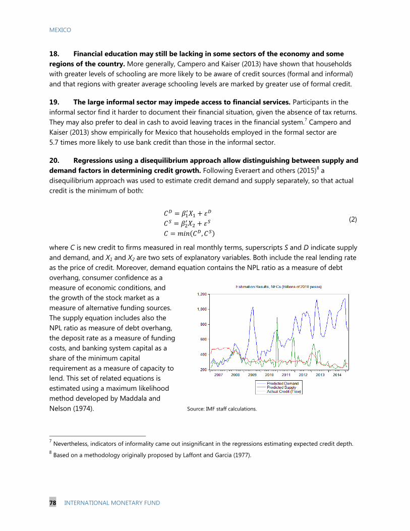
MEXICO
78 INTERNATIONAL MONETARY FUND
18. Financial education may still be lacking in some sectors of the economy and some
regions of the country. More generally, Campero and Kaiser (2013) have shown that households
with greater levels of schooling are more likely to be aware of credit sources (formal and informal)
and that regions with greater average schooling levels are marked by greater use of formal credit.
19. The large informal sector may impede access to financial services. Participants in the
informal sector find it harder to document their financial situation, given the absence of tax returns.
They may also prefer to deal in cash to avoid leaving traces in the financial system.7 Campero and
Kaiser (2013) show empirically for Mexico that households employed in the formal sector are
5.7 times more likely to use bank credit than those in the informal sector.
20. Regressions using a disequilibrium approach allow distinguishing between supply and
demand factors in determining credit growth. Following Everaert and others (2015)8 a
disequilibrium approach was used to estimate credit demand and supply separately, so that actual
credit is the minimum of both:
where C is new credit to firms measured in real monthly terms, superscripts S and D indicate supply
and demand, and X1 and X2 are two sets of explanatory variables. Both include the real lending rate
as the price of credit. Moreover, demand equation contains the NPL ratio as a measure of debt
overhang, consumer confidence as a
measure of economic conditions, and
the growth of the stock market as a
measure of alternative funding sources.
The supply equation includes also the
NPL ratio as measure of debt overhang,
the deposit rate as a measure of funding
costs, and banking system capital as a
share of the minimum capital
requirement as a measure of capacity to
lend. This set of related equations is
estimated using a maximum likelihood
method developed by Maddala and
Nelson (1974).
7 Nevertheless, indicators of informality came out insignificant in the regressions estimating expected credit depth.
8 Based on a methodology originally proposed by Laffont and Garcia (1977).
(2)
Source: IMF staff calculations.

MEXICO
INTERNATIONAL MONETARY FUND 79
21. An analysis of supply and demand for credit suggests that in recent years, credit was
mostly supply driven. Since 2008, credit supply has been insufficient to meet demand by about
MXN (of 2010) 300 billion in recent months. While the estimated figures for the gap between
demand and supply are quite sensitive to the explanatory variables used, the general finding of
supply-driven credit flows remains robust over many possible choices.
D. Current Trends and Policies
22. Measures taken in response to the 1994 foreign currency crisis, as well as more recent
reforms can be expected to increase trust in the banking system.
The Bank of Mexico tightened the regulation on net open foreign currency positions following
the 1994 crisis to close the loophole that allowed banks circumventing it by using derivatives or
off-balance sheet positions.
Financial regulation has been strengthened over the years, and Mexico has been fast in adopting
Basel III accord standards, with both the risk-based capital and the liquidity rules assessed as
compliant (Basel Committee on Banking Supervision, 2015). The Liquidity Coverage Ratio applies
from 2015 and is phased in according to the Basel implementation schedule reaching the final
value of 100 percent in 2019.
A new deposit insurance institution (IPAB) was set up in 1999. This now insures deposits of up to
MXN 2.1 million,9 which is clearer and more credible than the previous system, which did not
have an explicit limit.
23. Difficulties in monitoring credit quality and obtaining access to collateral are being
addressed.
The 2014 financial reform created a new legal instrument to allow for quicker execution of client
collateral in case of default. As a result of this and other changes, in the World Bank’s (2014)
Doing Business data, Mexico’s distance to frontier indicator for resolving bankruptcy improved
by 6.5 percentage points.
More mercantile matters, such as loans involving physical collateral, will be shifted to federal
courts, but this is not implemented yet.
Information sharing between the private credit bureaus is improved and will contain information
from the public mortgage lenders (Infonavit and FOVISSSTE) in addition to information from
private banks.
9 Legally it is fixed in the inflation-adjusted units of account (Unidad de Inversion, UDI) at a level of 400,000 UDIs.
MEXICO
80 INTERNATIONAL MONETARY FUND
24. Financial education is being strengthened.
CONDUSEF, the financial consumer protection agency provides various online tools. A new
Financial Entities Bureau will facilitate product comparisons across financial entities. It already
allows a broad comparison of banks and lists abusive clauses and bad practices.
The move toward cashless salaries and benefits10
familiarizes recipients with financial services.
A more general education reform aims at improving the quality of education.
25. Competition in the banking sector is supported by various measures of the 2014
financial reform. These include new provisions that facilitate the portability of bank accounts and
mortgages between banks. Moreover, transparency has been improved by obliging banks to publish
comparable interest rates.
26. The Secretary of Finance has been given the mandate to assess compliance of banks
with their objective to support and promote productive sectors and domestic economic
growth in accordance to best practices and banking guidelines. The first report will be prepared
during 2016 and contain recommendations. Banks which are assessed as providing insufficient credit
will have to prepare action plans to address this.
27. At current credit growth rates, credit depth is increasing gradually and this pace seems
appropriate.
The current growth rate of around 10 percent exceeds the rate of nominal GDP growth. While
rising credit to GDP shares are sometimes considered a warning sign, in the case of Mexico this
is welcome after years of weak credit. According to estimates by Arcand and others (2015),
increasing the share of bank credit by 1 percentage point of GDP to 18 percent of GDP (as
forecast for 2016), would boost growth by 0.03 percentage points. Increasing the ratio of bank
credit to GDP to 60 percent, would boost growth rates by 0.8 percentage points.
At the current credit growth rate of around 10 percent, and assuming nominal growth of
6.4 percent over the medium term (potential growth of 3.3 percent and 3 percent inflation), the
predicted bank credit ratio of 60 percent of GDP would be reached in 37 years. Boosting the
credit growth rate to 15 percent would reduce this time frame to 16 years. An even faster
growth rate would be risky. Sahay and others (2015) shows that financial deepening at a fast
pace leads to increased growth volatility and financial instability.
10
See Babatz (2013) for details on this shift.

MEXICO
INTERNATIONAL MONETARY FUND 81
0
2
4
6
8
10
12
14
-40
-20
0
20
40
60
80
2004 2006 2008 2010 2012 2014
Credit NPLs (in percent of credit, RHS)
Credit Card Debt(Y/Y monthly growth, in percent)
Sources: National authorities; and IMF staff calculations.
28. Despite the overall low level of credit depth, some sectors have seen excessive growth
and subsequent problems. Consumer credit—
especially credit cards—has seen large growth
rates between 2004 and 2007, but standards
were low and the quality of credit fell. A rise in
nonperforming loans put a stop to the
expansion in 2008. In annual terms, credit
contracted every month from September 2009
through March 2011. Nonperforming credit card
loans rose from 3.1 percent of credit in January
2004 to a peak of 12.6 percent in May 2009.
E. Conclusions
29. Credit depth has been exceptionally low in Mexico for decades, but credit growth is
recovering. The key challenge going forward will be to encourage further credit expansion without
jeopardizing financial stability. This will require a continuation of tight regulation, maintaining high
credit standards, and avoiding excessively rapid credit growth.
30. Given the history of bank crises, it is paramount to build up a resilient financial sector
in which lenders and borrowers have full trust. The strong financial regulation should therefore
be maintained and must not be sacrificed in an attempt to boost credit.
31. Empirical evidence supports the idea that structural aspects of the banking sector are
behind the low degree of financial intermediation. This is suggested both by results showing
that credit growth has been supply-driven in recent years, and by the apparent lagging of credit
cycles with respect to real cycles.
32. The financial reforms over the last few years address the weaknesses, but must be
strongly implemented and further evolutionary changes will be needed.
The shifting of more mercantile matters to federal courts, which is essential for improving
bankruptcy procedures and collateral recovery, has been delayed and should be urgently
implemented.
The IPAB needs to be put on a stronger financial footing to strengthen its credibility, as the fund
now contains just a very small percentage of the insured deposits.
The new mandate that allows the Finance Secretary to scrutinize banks’ compliance with their
mandates could be risky depending on its implementation. The perception of putting pressure
on banks to increase lending could have negative financial stability consequences, although the
strong regulatory standards provide protection.
The international financial system is undergoing continuous reform, with Basel III still not
completely agreed among the Basel Committee members. Mexico will have to follow these
developments and ensure that Mexican law evolves in line.

MEXICO
82 INTERNATIONAL MONETARY FUND
References
Angeles, Luis, 2015, “Credit Expansion and the Economy,” Applied Economics Letters, Vol. 22(13), pp.
1064-1072.
Arcand, Jean Louris, Enrico Berkes, and Ugo Panizza, 2015, “Too Much Finance?” Journal of Economic
Growth, Vol. 20, pp. 105-148.
Babatz, Guillermo, 2013, “Sustained Effort, Saving Billions: Lessons from the Mexican Government’s
Shift to Electronic Payments,” Better than Cash Alliance, Evidence Paper.
Banco de Mexico, 2010, “Reporte sobre el Sistema Financiero,” Mexico, D.F.
Basel Committee on Banking Supervision, 2015, “Eighth Progress Report on Adoption of the Basel
Regulatory Framework,” Bank for International Settlements.
Campero, Alejandra and Karen Kaiser, 2013, “Access to Credit: Awareness and Use of Formal and
Informal Credit Institutions,” Banco de Mexico Working Papers, No. 2013-07.
Claessens, Stijn, and Luc Laeven, 2004, “What Drives Bank Competition? Some International
Evidence,” Journal of Money, Credit and Banking, Vol. 36, No. 3, Pt. 2, pp. 563-583.
Cottarelli, Carlo, Giovanni Dell’Ariccia, and Ivanna Vladkova-Hollar, 2004, “Early Birds, Late Risers,
and Sleeping Beauties: Bank Credit Growth to the Private Sector in Central and Eastern Europe and
in the Balkans,” Journal of Banking and Finance, Vol. 29, pp. 83-104.
Everaert, Greetje, Natasha Che, Nan Geng, Bertrand Gruss, Gregorio Impavido, Yinqiu Lu, Christian
Saborowski, Jerome Vandenbusche, and Li Zeng, 2015, “Does Supply or Demand Drive the Capital
Cycle? Evidence from Central, Eastern and Southeastern Europe,” IMF Working Papers, No. 15/15.
Gourinchas, Pierre-Olivier and Maurice Obstfeld, 2012, “Stories of the Twentieth Century for the
Twenty-First,” American Economic Journal: Macroeconomics, Vol. 4(1), pp. 226-265.
Graf, Pablo, 1999, “Policy Response to the Banking Crisis in Mexico,” in: Bank for International
Settlements, Bank Restructuring in Practice, BIS Policy Papers, No. 6, pp. 164-182.
Hansen, Niels Jakob H. and Olga Sulla, 2013, „Credit Growth in Latin America: Financial Development
or Credit Boom,” IMF Working Papers, No. 13/106.
Heng, Dyna, Anna Ivanova, Rodrigo Mariscal, Uma Ramakrishnan, and Joyce Cheng Wong, 2015,
“Advancing Financial Development in Latin America and the Caribbean,” in: Western Hemisphere
Regional Economic Outlook—Adjusting Under Pressure, Chapter 5, pp. 75-87, International
Monetary Fund.

MEXICO
INTERNATIONAL MONETARY FUND 83
Laeven, Luc and Fabian Valencia, 2012, “Systemic Banking Crises Database: An Update,” IMF
Working Papers, No. 12/163.
Laffont, Jean-Jacques and Rene Garcia, 1977, “Disequilibrium Econometrics for Business Loans,”
Econometrica, Vol. 45, pp. 1187-1120.
McQuerry, Elizabeth, 1999, “the Banking Sector Rescue in Mexico,” Federal Reserve Bank of Atlanta
Economic Review, Third Quarter 1999.
Maddala, Ganggadharrao and Forrest Nelson, 1974, “Maximum Likelihood Methods for Models of
Market Disequilibrium,” Econometrica, Vol. 42(6), pp. 1013-1030.
Sahay, Ratna, Martin Cihak, Papa N’Diaye, Adolfo Barajas, Ran Bi, Diana Ayala, Yuan Gao, Annette
Kyobe, Lam Nguyen, Christian Saborowski, Katsiaryna Svirydzenka, and Seyed Reza Yousefi, 2015,
“Rethinking Financial Deepening: Stability and Growth in Emerging Markets,” IMF Staff Discussion
Note, No. 15/08.
World Bank, 2014, “Doing Business 2015: Going Beyond Efficiency,” Washington, DC: World Bank
Group.