Housing Price and Household Debt Interactions in … Price and Household Debt Interactions in Sweden...

WP/15/276

Housing Price and Household Debt Interactions in Sweden

by Rima A. Turk

© 2015 International Monetary Fund WP/15/276

IMF Working Paper

European Department

Housing Price and Household Debt Interactions in Sweden

Prepared by Rima A. Turk

Authorized for distribution by Craig Beaumont

December 2015

Abstract

Sweden is experiencing double-digit housing price gains alongside rising household debt. A common interpretation is that mortgage lending boosted by expansionary monetary policy is driving up house prices. But theory suggests the value of housing collateral is also important for household’s capacity to borrow. This paper examines the interactions between housing prices and household debt using a three-equation model, finding that household borrowing impacts housing prices in the short-run, but the price of housing is the main driver of the secular trend in household debt over the long-run. Both housing prices and household debt are estimated to be moderately above their long-run equilibrium levels, but the adjustment toward equilibrium is not found to be rapid. Whereas low interest rates have contributed to the recent surge in housing prices, growth in incomes and financial assets play a larger role. Policy experiments suggest that a gradual phasing out of mortgage interest deductibility is likely to have a manageable effect on housing prices and household debt.

JEL Classification Numbers: E21, E41; E51; R21.

Keywords: Housing market, Household debt, Collateral, Sweden.

Author’s E-Mail Address: [email protected]

IMF Working Papers describe research in progress by the author(s) and are published to elicit comments and to encourage debate. The views expressed in IMF Working Papers are those of the author(s) and do not necessarily represent the views of the IMF, its Executive Board, or IMF management.

2

Contents

I. INTRODUCTION ________________________________________________________4

II. HOUSING AND MORTGAGE MARKETS IN SWEDEN ______________________6

III. SUMMARY OF RELATED LITERATURE _______________________________12

IV. MODELING FRAMEWORK AND DATA _________________________________16

V. EMPIRICAL FINDINGS ________________________________________________23

VI. POLICY ANALYSIS ___________________________________________________33

VII. CONCLUSIONS AND POLICY IMPLICATIONS _________________________36

REFERENCES ___________________________________________________________37

BOX 1. Housing Supply and Rent Controls in Sweden _________________________________41 FIGURES 1. Real Housing Prices, Household Debt, and Disposable Income _____________________4 2. Growth in Real Housing Prices and Real Household Debt Per Capita_________________5 3. Housing Completions and Change in Population _________________________________7 4. Residential Investment _____________________________________________________8 5. Housing Supply: Sweden vs. Urban cities ______________________________________8 6. Type of Dwellings_________________________________________________________9 7. Tenure of Apartments ______________________________________________________9 8. Household Debt to Disposable Income ________________________________________10 9. Household Debt Ratios ____________________________________________________11 10. Household Debt ________________________________________________________11 11. Tax Incentives for Home Ownership ________________________________________12 12. Conceptual Overview:3-Equation Model ____________________________________20 13. Real Housing Prices: Actual vs. Long Run Fitted _____________________________24 14. Housing Price Model Predictability _________________________________________24 15. Contribution of Fundamentals to Housing Prices ______________________________26 16. Housing Price Deviation from Fundamentals ________________________________27 17. Real Household Debt: Actual vs. Long Run Fitted _____________________________30 18. Contribution of Fundamentals to Household Debt _____________________________30 19. Household Debt Deviation from Fundamentals ______________________________30 20. Dynamics: Growth in Real Housing Prices and Real Household Debt _____________32 21. Outlook for the Debt-to-Income Ration _____________________________________32 22. Impact of Increasing Housing Supply on Real Housing Prices ___________________34 23. Simulation 1: Mortgage Deductibility Reduction from 30 to 20 percent over 1 year ___35 24. Simulation 2: Phasing-Out Mortgage Deductibility by 5 ppts p.a. over 6 years ______35

3

25. Simulation 3: Normalization after a Prolonged Period of Low Interest _____________36 TABLES 1. Brief Summary of the Literature _____________________________________________14 2. Variables Definition and Data Sources ________________________________________21 3. Summary Statistics _______________________________________________________22 4. Unit Root Tests __________________________________________________________22 5. LR Cointengrating Relationship: Real Housing Prices ___________________________23 6. Selected Findings from the Literature _________________________________________25 7. Short-Run Dynamics: Real Housing Prices ____________________________________27 8. LR Cointegrating Relationship: Real Household Debt ____________________________29 9. Short-Run Dynamics: Real Household Debt ___________________________________31 10. Residential Investment ___________________________________________________33 ANNEX I. Robustness Checks _______________________________________________________42 ANNEX TABLES A1. Cointegrating Relationship: Real Housing Prices, Robustness Tests _______________43 A2. Cointegrating Relationship: Real Household Debt Per Capita, Robustness Tests _____43

4

I. INTRODUCTION1

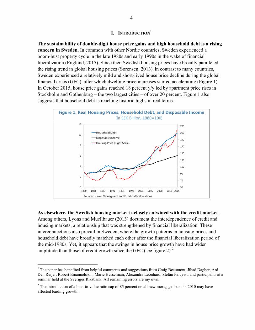
The sustainability of double-digit house price gains and high household debt is a rising concern in Sweden. In common with other Nordic countries, Sweden experienced a boom-bust property cycle in the late 1980s and early 1990s in the wake of financial liberalization (Englund, 2015). Since then Swedish housing prices have broadly paralleled the rising trend in global housing prices (Sørensen, 2013). In contrast to many countries, Sweden experienced a relatively mild and short-lived house price decline during the global financial crisis (GFC), after which dwelling price increases started accelerating (Figure 1). In October 2015, house price gains reached 18 percent y/y led by apartment price rises in Stockholm and Gothenburg – the two largest cities – of over 20 percent. Figure 1 also suggests that household debt is reaching historic highs in real terms.

Figure 1. Real Housing Prices, Household Debt, and Disposable Income (In SEK Billion; 1980=100)

As elsewhere, the Swedish housing market is closely entwined with the credit market. Among others, Lyons and Muellbauer (2013) document the interdependence of credit and housing markets, a relationship that was strengthened by financial liberalization. These interconnections also prevail in Sweden, where the growth patterns in housing prices and household debt have broadly matched each other after the financial liberalization period of the mid-1980s. Yet, it appears that the swings in house price growth have had wider amplitude than those of credit growth since the GFC (see figure 2).2

1 The paper has benefited from helpful comments and suggestions from Craig Beaumont, Jihad Dagher, Ard Den Reijer, Robert Emanuelsson, Marie Hesselman, Alexandra Leonhard, Stefan Palqvist, and participants at a seminar held at the Sveriges Riksbank. All remaining errors are my own. 2 The introduction of a loan-to-value ratio cap of 85 percent on all new mortgage loans in 2010 may have affected lending growth.

50

70

90

110

130

150

170

190

210

230

0

2

4

6

8

10

12

1980 1984 1987 1991 1994 1998 2001 2005 2008 2012

Household Debt

Disposable Income

Housing Price (Right Scale)

Sources: Haver, Valueguard, and Fund staff calculations.

2015

5

Figure 2. Growth in Real Housing Prices and Real Household Debt Per Capita (In Percent)

A common interpretation of the link between these markets is that mortgage lending drives housing prices up, motivating measures to curb credit. Relaxing the credit constraint on households through higher access to residential mortgage lending (see Bernanke and Gertler, 1995; Kiyotaki and Moore, 1997) puts upward pressure on housing prices in the presence of inelastic housing supply in the short run. Under good credit conditions, the slow development of financial distortions is masked by favorable economic conditions and the lower perception of risk eventually channels distortions to the real economy (Borio and Lowe, 2002). The recognition that risks can build up in the financial sector over time has motivated the use of macroprudential instruments to improve financial sector resilience to shocks (IMF, Global Financial Stability Report, 2011).

Yet, mortgage lending can also be driven by rising housing prices through the wealth and collateral channels. Home ownership generally requires debt financing, especially as households usually acquire this major asset early in their life cycle. When house prices appreciate, households who own housing may perceive that their higher wealth allows for greater lifetime consumption, inducing households to borrow and spend more. At the same time, the higher value of housing assets expands the value of collateral against which borrowing is generally much cheaper than unsecured credit. Relaxing this collateral constraint thereby expands households’ borrowing capacity, which could be reflected in a combination of higher consumption and larger asset holdings. For households that do not yet own a house, higher prices increase the need to borrow but also relax collateral constraints (Greenspan and Kennedy, 2008; Mian and Sufi, 2011).3

3 Since housing assets constitute a large fraction of household net wealth, housing prices may also explain household saving and consumption patterns. For the effect of house price dynamics on broad economic outcomes, see Berg and Bergström (1995).

-20

-15

-10

-5

0

5

10

15

20

1981:1 1988:1 1995:1 2002:1 2009:1

Real Housing Prices

Real HH Debt pc

Sources: Haver, Statistics Sweden, and fund staff calculations 2015q2

6

In modeling the interaction of housing prices and household debt in Sweden, this paper seeks to allow for effects to run in both directions. The analysis investigates the long-run drivers and short-term dynamics of both housing prices and household debt in Sweden, using a simple three-equation model where residential investment is also endogenous. The main finding is the large role of the value of housing collateral in driving the secular trend in household debt since financial liberalization in the mid 1980s. These rises in collateral value are primarily driven by housing prices, trends in which are found to be well explained by fundamentals, yet credit growth does play a significant role in the short-run dynamics of housing prices.

The study’s contributions are threefold. It first contributes to the literature on the interdependence between housing market outcomes and mortgage credit by providing evidence from Sweden. It also extends the interaction effects between housing prices and household debt to allow for feedback from housing prices to residential investment. Finally, it provides empirical evidence on the importance of the collateral channel in driving household debt.

The remainder of the paper is structured as follows. Section II describes the key features of the housing and mortgage markets in Sweden, noting the timing and nature of major developments. Section III briefly reviews the related literature. Section IV presents the modeling framework and section V discusses the data and empirical results. Section VI illustrates the dynamic response of housing prices and household debt to shocks and section VII concludes and offers some policy recommendations.

II. HOUSING AND MORTGAGE MARKETS IN SWEDEN

Sweden’s housing market developments reflect the intersection of evolving supply and demand factors. As discussed in section V, rising incomes and demographics have increased housing demand over the past few decades. Sweden’s housing supply growth was shaped by variations in government support for construction and by the boom-bust cycle after financial liberalization. Rent controls have limited the availability of rental housing, adding to the demand for owner-occupied housing. At the same time, low rents owing to the controls have encouraged the conversion of rental apartments to tenant ownership, thereby contributing to increasing home ownership in Sweden. Despite the financial liberalization, households generally borrow only in relation to housing they occupy, including vacation homes, with little of the “buy-to-let” borrowing activity seen in other advanced economies.

Housing Market

Sweden’s housing supply was substantially affected by evolving government policies and a boom-bust cycle from the mid-1980s. Historically, the Swedish government had substantial influence over housing construction, supporting intensive construction, especially

7

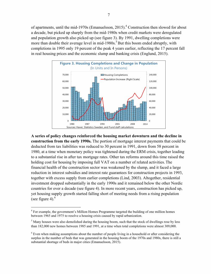
of apartments, until the mid-1970s (Emanuelsson, 2015).4 Construction then slowed for about a decade, but picked up sharply from the mid-1980s when credit markets were deregulated and population growth also picked up (see figure 3). By 1991, dwelling completions were more than double their average level in mid-1980s.5 But this boom ended abruptly, with completions in 1995 only 19 percent of the peak 4 years earlier, reflecting the 17 percent fall in real housing prices and the economic slump and banking crisis (Englund, 2015).

Figure 3. Housing Completions and Change in Population (In Units and In Persons)

A series of policy changes reinforced the housing market downturn and the decline in construction from the early 1990s. The portion of mortgage interest payments that could be deducted from tax liabilities was reduced to 30 percent in 1991, down from 58 percent in 1980, at a time when monetary policy was tightened during the ERM crisis, together leading to a substantial rise in after tax mortgage rates. Other tax reforms around this time raised the holding cost for housing by imposing full VAT on a number of related activities. The financial health of the construction sector was weakened by the slump, and it faced a large reduction in interest subsidies and interest rate guarantees for construction projects in 1993, together with excess supply from earlier completions (Lind, 2003). Altogether, residential investment dropped substantially in the early 1990s and it remained below the other Nordic countries for over a decade (see figure 4). In more recent years, construction has picked up, yet housing supply growth started falling short of meeting needs from a rising population (see figure 4).6

4 For example, the government’s Million Homes Programme targeted the building of one million homes between 1965 and 1975 to resolve a housing crisis caused by rapid urbanization. 5 Many houses were also demolished during the housing boom, such that the stock of dwellings rose by less than 182,000 new homes between 1985 and 1991, at a time when total completions were almost 309,000.

6 Even when making assumptions about the number of people living in a household or after considering the surplus in the number of beds that was generated in the housing boom of the 1970s and 1980s, there is still a substantial shortage of beds in major cities (Emanuelsson, 2015).

0

20,000

40,000

60,000

80,000

100,000

120,000

140,000

0

10,000

20,000

30,000

40,000

50,000

60,000

70,000

1980 1987 1994 2001 2008

Housing Completions

Population Increase (Right Scale)

Sources: Haver, Statistics Sweden, and Fund staff calculations2014

8

Figure 4. Residential Investment

(In Percent of GDP)

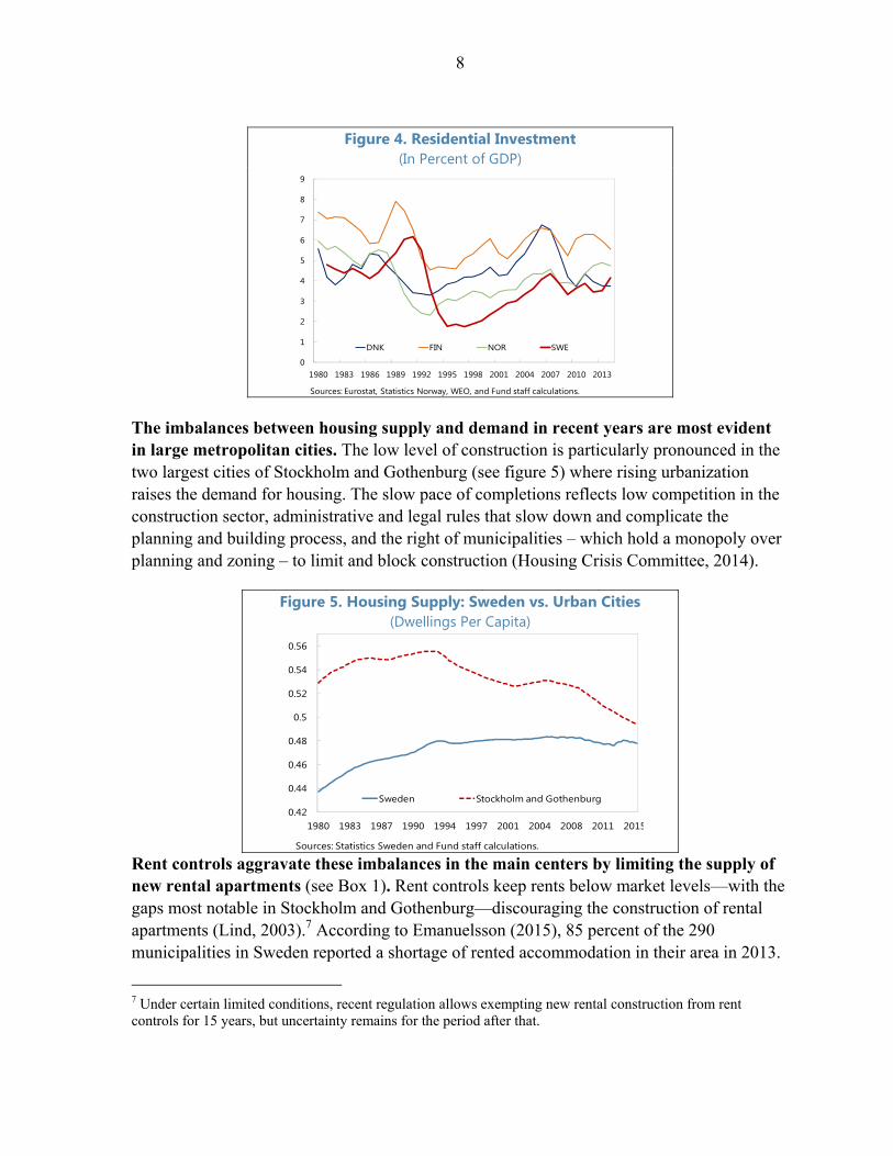
The imbalances between housing supply and demand in recent years are most evident in large metropolitan cities. The low level of construction is particularly pronounced in the two largest cities of Stockholm and Gothenburg (see figure 5) where rising urbanization raises the demand for housing. The slow pace of completions reflects low competition in the construction sector, administrative and legal rules that slow down and complicate the planning and building process, and the right of municipalities – which hold a monopoly over planning and zoning – to limit and block construction (Housing Crisis Committee, 2014).

Figure 5. Housing Supply: Sweden vs. Urban Cities (Dwellings Per Capita)

Rent controls aggravate these imbalances in the main centers by limiting the supply of new rental apartments (see Box 1). Rent controls keep rents below market levels—with the gaps most notable in Stockholm and Gothenburg—discouraging the construction of rental apartments (Lind, 2003).7 According to Emanuelsson (2015), 85 percent of the 290 municipalities in Sweden reported a shortage of rented accommodation in their area in 2013.

7 Under certain limited conditions, recent regulation allows exempting new rental construction from rent controls for 15 years, but uncertainty remains for the period after that.

0

1

2

3

4

5

6

7

8

9

1980 1983 1986 1989 1992 1995 1998 2001 2004 2007 2010 2013

DNK FIN NOR SWE

Sources: Eurostat, Statistics Norway, WEO, and Fund staff calculations.

0.42

0.44

0.46

0.48

0.5

0.52

0.54

0.56

1980 1983 1987 1990 1994 1997 2001 2004 2008 2011 2015

Sweden Stockholm and Gothenburg

Sources: Statistics Sweden and Fund staff calculations.

9

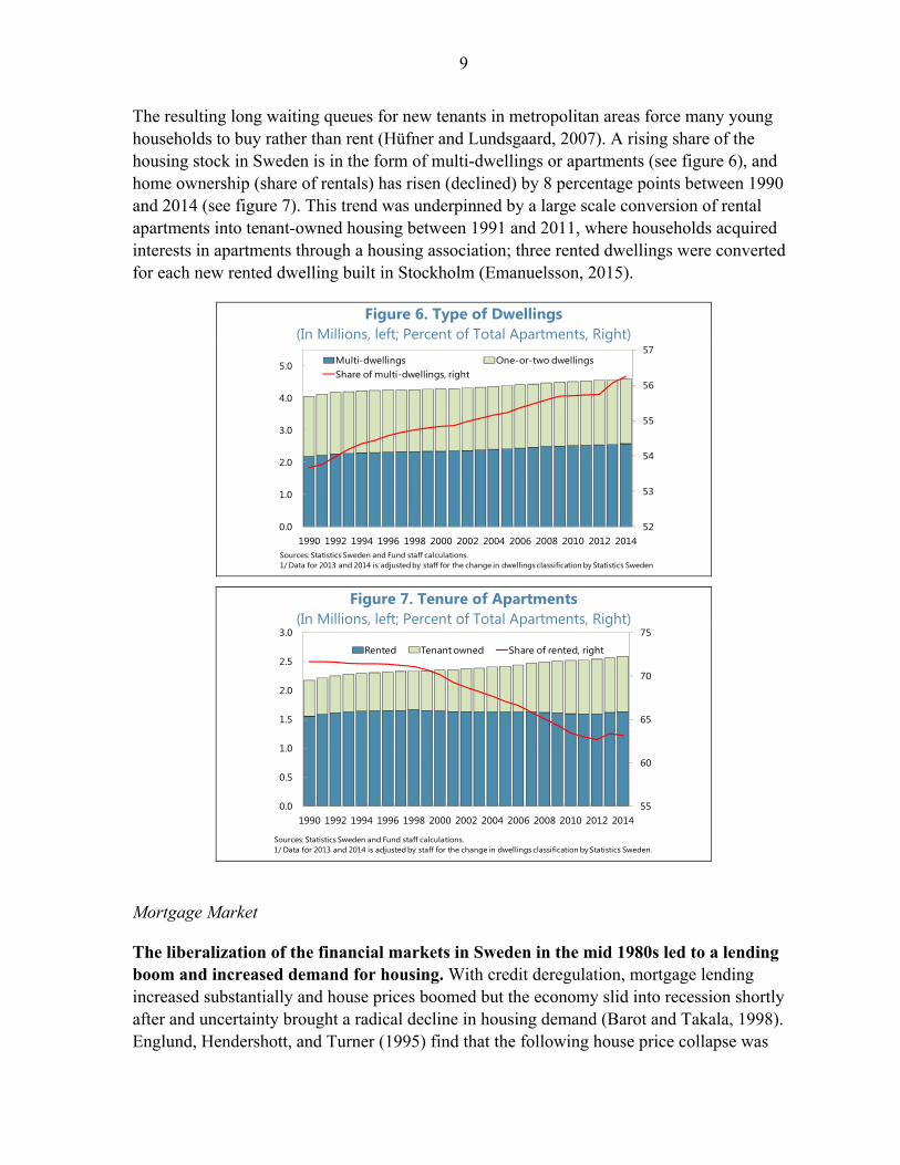
The resulting long waiting queues for new tenants in metropolitan areas force many young households to buy rather than rent (Hüfner and Lundsgaard, 2007). A rising share of the housing stock in Sweden is in the form of multi-dwellings or apartments (see figure 6), and home ownership (share of rentals) has risen (declined) by 8 percentage points between 1990 and 2014 (see figure 7). This trend was underpinned by a large scale conversion of rental apartments into tenant-owned housing between 1991 and 2011, where households acquired interests in apartments through a housing association; three rented dwellings were converted for each new rented dwelling built in Stockholm (Emanuelsson, 2015).

Figure 6. Type of Dwellings (In Millions, left; Percent of Total Apartments, Right)

Figure 7. Tenure of Apartments

(In Millions, left; Percent of Total Apartments, Right)

Mortgage Market

The liberalization of the financial markets in Sweden in the mid 1980s led to a lending boom and increased demand for housing. With credit deregulation, mortgage lending increased substantially and house prices boomed but the economy slid into recession shortly after and uncertainty brought a radical decline in housing demand (Barot and Takala, 1998). Englund, Hendershott, and Turner (1995) find that the following house price collapse was

52

53

54

55

56

57

0.0

1.0

2.0

3.0

4.0

5.0

1990 1992 1994 1996 1998 2000 2002 2004 2006 2008 2010 2012 2014

Multi-dwellings One-or-two dwellingsShare of multi-dwellings, right

Sources: Statistics Sweden and Fund staff calculations. 1/ Data for 2013 and 2014 is adjusted by staff for the change in dwellings classification by Statistics Sweden.

55

60

65

70

75

0.0

0.5

1.0

1.5

2.0

2.5

3.0

1990 1992 1994 1996 1998 2000 2002 2004 2006 2008 2010 2012 2014

Rented Tenant owned Share of rented, right

Sources: Statistics Sweden and Fund staff calculations. 1/ Data for 2013 and 2014 is adjusted by staff for the change in dwellings classification by Statistics Sweden.

10

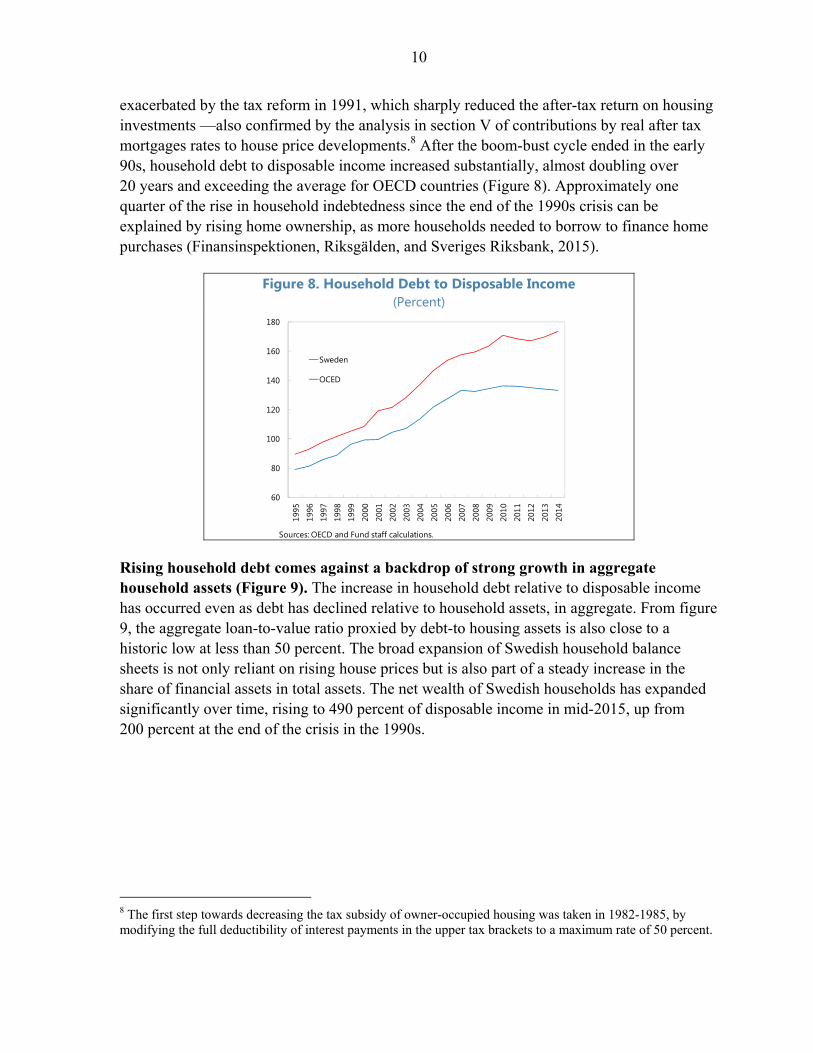
exacerbated by the tax reform in 1991, which sharply reduced the after-tax return on housing investments —also confirmed by the analysis in section V of contributions by real after tax mortgages rates to house price developments.8 After the boom-bust cycle ended in the early 90s, household debt to disposable income increased substantially, almost doubling over 20 years and exceeding the average for OECD countries (Figure 8). Approximately one quarter of the rise in household indebtedness since the end of the 1990s crisis can be explained by rising home ownership, as more households needed to borrow to finance home purchases (Finansinspektionen, Riksgälden, and Sveriges Riksbank, 2015).

Figure 8. Household Debt to Disposable Income (Percent)

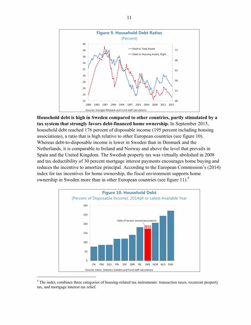
Rising household debt comes against a backdrop of strong growth in aggregate household assets (Figure 9). The increase in household debt relative to disposable income has occurred even as debt has declined relative to household assets, in aggregate. From figure 9, the aggregate loan-to-value ratio proxied by debt-to housing assets is also close to a historic low at less than 50 percent. The broad expansion of Swedish household balance sheets is not only reliant on rising house prices but is also part of a steady increase in the share of financial assets in total assets. The net wealth of Swedish households has expanded significantly over time, rising to 490 percent of disposable income in mid-2015, up from 200 percent at the end of the crisis in the 1990s.

8 The first step towards decreasing the tax subsidy of owner-occupied housing was taken in 1982-1985, by modifying the full deductibility of interest payments in the upper tax brackets to a maximum rate of 50 percent.

60

80

100

120

140

160

180

1995

1996

1997

1998

1999

2000

2001

2002

2003

2004

2005

2006

2007

2008

2009

2010

2011

2012

2013

2014

Sweden

OCED

Sources: OECD and Fund staff calculations.

11

Figure 9. Household Debt Ratios (Percent)

Household debt is high in Sweden compared to other countries, partly stimulated by a tax system that strongly favors debt-financed home ownership. In September 2015, household debt reached 176 percent of disposable income (195 percent including housing associations), a ratio that is high relative to other European countries (see figure 10). Whereas debt-to-disposable income is lower in Sweden than in Denmark and the Netherlands, it is comparable to Ireland and Norway and above the level that prevails in Spain and the United Kingdom. The Swedish property tax was virtually abolished in 2008 and tax deductibility of 30 percent mortgage interest payments encourages home buying and reduces the incentive to amortize principal. According to the European Commission’s (2014) index for tax incentives for home ownership, the fiscal environment supports home ownership in Sweden more than in other European countries (see figure 11).9

Figure 10. Household Debt (Percent of Disposable Income), 2014q4 or Latest Available Year

9 The index combines three categories of housing-related tax instruments: transaction taxes, recurrent property tax, and mortgage interest tax relief.

48

53

58

63

68

73

22

24

26

28

30

32

34

36

38

40

1980 1983 1987 1990 1994 1997 2001 2004 2008 2011 2015

Debt to Total Assets

Debt to Housing Assets, Right

Sources: Sveriges Riksbank and Fund staff calculations

0

50

100

150

200

250

300

ITA FRA DEU FIN ESP GBR IRL SWE NOR NLD DNK

Sources: Haver, Statistics Sweden,and Fund staff calculations

Debt of tenant-owned associations

12

Figure 11. Tax Incentives for Home Ownership Composite Tax Index Range: 0 (Low) to 2 (High)

III. SUMMARY OF RELATED LITERATURE

Drawing on the literature discussed below, this paper uses a three-equation model to represent the housing and debt markets. The equations reflect housing prices, household debt, and residential investment. A more comprehensive representation of the housing market is found in MOSES, which is a small aggregate econometric model for studying the Swedish economy (Bårdsen, den Reijer, Jonasson, and Nymoen, 2012).

Housing prices

Following Meen (2002), housing prices are often modeled using an inverted demand curve. The fundamental drivers of housing demand considered in the literature include household income, the real user cost of housing, and demographic factors such as the age structure of the population. Housing supply typically adjusts slowly to changes in demand, as construction takes time and is generally small relative to the existing stock, hence supply conditions also shape housing prices. Since the housing market is relatively illiquid compared with other asset markets and price adjustments to demand and supply shocks also take time, housing price dynamics are widely modeled using an Error Correction Model (ECM) specification.

There is a rich literature on the economic determinants of real housing prices, including papers for Sweden. Among studies focusing on Sweden, Hort (1998) examines speculative behavior in the housing market, Barot (2001) and Barot and Yang (2002) investigate housing demand and supply determinants. More recently, Claussen (2013) finds that rising disposable income and falling mortgage rates explain the upswing in housing prices, with no evidence of overpricing. Interest in housing price cycles was renewed in the aftermath of the global financial crisis not just for Sweden but also in a cross country context (Caldera Sánchez and

0

0.5

1

1.5

2

2.5

FRA GBR ITA ESP DEU IRL DEN NLD FIN SWE

2011

2013

Sources: European Commission and Fund staff calculations.

13

Johansson, 2011). Table 1 provides a summary of research for Sweden and selected work for other advanced economies.

The long run effect of real interest rates on housing prices differs across studies.10 For papers on Sweden, the estimated semi-elasticity of housing prices with respect to interest rates varies from close to 0 percent (Caldera Sánchez and Johansson, 2011) to 1-3 percent (Hort, 1998; Barot, 2001; Barot and Yang, 2002), with the highest reported coefficient at 6 percent (Claussen, 2013).11 For studies on other advanced countries, the semi-elasticity of real housing prices with respect to interest rates ranges between 0.1 to 3.2 percent (Andrews, 2010; Gimeno and Martinez-Carrascal, 2010; Adams, Zeno and Roland Füss; 2010). These results provide a benchmark for assessing estimates presented later.

A number of studies for other countries provide empirical evidence on the interdependence between housing market outcomes and mortgage credit.12 Oikarinen (2009a and b) and Anundsen and Jansen (2013) find strong evidence of a two-way interaction between housing prices and loans in Finland and Norway, respectively; Gimeno and Martinez-Carrascal (2010) show that causality in Spain runs from house purchase loans to house prices; and Lyons and Muellbauer (2013) document that credit conditions matter for the housing market in Ireland.13 This paper contributes to this literature by providing similar evidence from Sweden.

Household debt

The collateral channel is thoroughly examined in the literature. The role of collateral is well documented in the corporate finance literature (Barro, 1976; Stiglitz and Weiss, 1981; Hart and Moore; 1994; Kiyotaki and Moore, 1997; Chaney, Sraer, and Thesmar, 2012), in transmitting housing market shocks to the risk premia in asset markets (Lustig and van Nieuwerburgh, 2005), in smoothing household spending (Hurst and Stafford, 2004; Cooper, 2009), and in explaining medium-term consumption fluctuations (Iacoviello, 2004; Muellbauer and Murphy, 2008).

10 The after-tax real interest rate is the main factor shaping the user cost of housing, in addition to expected capital gains, given that housing taxes and capital depreciation usually exhibit inertia. 11 Some papers (Oikarinen, 2009a and b; Anundsen and Jansen, 2013) have questioned whether interest rates should enter a long-run house price equation. Still, Anundsen and Jansen (2013) document a response of housing prices to an interest rate shock, although the interest rate does not enter their short-run or long-run equation for housing prices directly. 12 Interest in the interaction between property valuation and credit is not limited to the housing sector. Davis and Zhu (2011) provide evidence on the reinforcing effects between commercial property cycles and aggregate bank lending. 13 Other studies have assessed the direction of causality between the property and credit market (e.g., Collyns and Senhadji, 2002; Gerlach and Peng, 2005; Liang and Cao, 2007), an issue which is not investigated in this paper.

Table 1. Brief Summary of the Literature

Paper Englund and Ioannides (1997) - Period: 1970q1-1992q4 (15 OECD countries, including Sweden).

Main Finding Strong first-order correlation in house price annual changes, and significant predictive power of GDP growth rate and real interest rate.

Method Patterns explaining house price changes, including autocorrelation and shocks that appear to drive house prices away from predicted values.

Dependent variable(s) House Price Changes

Level / LR variables N/A

Dynamic / SR variables Lags of house price changes and of GDP growth rate, real interest rate, and house prices.

Paper Hort, K. (1998) - Period: 1967-1994.

Main Finding Fundamentals explain well house price developments with autoregressive dynamics suggesting rapid adjustment, consistent with speculative behavior.

Method ECM framework: LR house price equation is first estimated, then residuals from the cointegrating regression are included in the SR dynamics.

Dependent variable(s) Real house prices.

Level / LR variables Real user cost of housing; real construction costs; real income; interest subsidies; net lending ratio; population 25-44 yrs, and first diffrences in RHS variables.

Dynamic / SR variables Sasme as LR variables, adding unemployment rate.

Paper Barot (2001) - Period: 1970h1-1997h2.

Main Finding Developments in house prices and housing investment can be explained by demand and supply fundamentals, including short-run adjustments in house prices.

Method ECM framework: Joint estimation of LR parameters and SR Dynamics for each of the demand and supply equations.

Dependent variable(s) (1) Demand side: Real house prices; (2) Supply side: Housing Investment scaled by GDP.

Level / LR variables (1)Debt to DI; debt to financial wealth; housing stock to income; rental housing to private stock; real after tax gvt bond rate; (2) Tobin's q; ST rate; tax reform dummy.

Dynamic / SR variables (1) Same as LR, adding population and rents; (2) same as LR.

Paper Barot and Yang (2002) - Period: 1970q1-1998q4.

Main Finding Comparison in Sweden and the UK reveals higher semi-elasticity for interest rates in Sweden and higher demand and supply speed of adjustment in the UK.

Method ECM framework: Joint estimation of LR parameters and SR Dynamics for each of the demand and supply equations.

Dependent variable(s) (1) Demand side: Real house prices; (2) Supply side: Housing Investment scaled by the housing stock.

Level / LR variables (1) Housing stock to DI; real after tax gvt bond rate; household financial wealth deflated by DI; debt deflated by DI; (2) Tobin's q.

Dynamic / SR variables (1) Rental stock; nominal LT gvt bond rate; nominal debt; employment; Population; tax reform dummy; (2) Tobin's q; GDP.

Paper Adams and Füss (2010) - Period: 1975q1-2007q2 (15 OECD countries, country by country analysis including Sweden).

Main Finding Macroeconomic variables significantly impact house prices, and speed of adjustment is slow (up to 14 years) in view of stickiness in residential house prices.

Method ECM framework: LR fundamentals modeled using DOLS and SR dynamics are assessed country by country.

Dependent variable(s) House price.

Level / LR variables Indicator of economic activity; long-term interest rates; construction costs.

Dynamic / SR variables Same as LR variables.

Paper Caldera Sánchez and Johansson (2011) - Period:1975q4-2008q4 (21 OECD countries, country by country analysis including Sweden).

Main Finding Housing supply responsivess to price changes is higher in some Nordic countries than in Europe, and depends on policies for land use and planning regulations.

Method ECM framework: Seemingly Unrelated Regression (SUR) simultaneous estimation for LR and SR equations.

Dependent variable(s) (1) Real house price; (2) Residential investment.

Level / LR variables (1) Real income; real interest rate; dwelling stock; population 25-44 yrs; (2) Construction costs; population 25-44 yrs.


Panel A: Sweden Studies

14

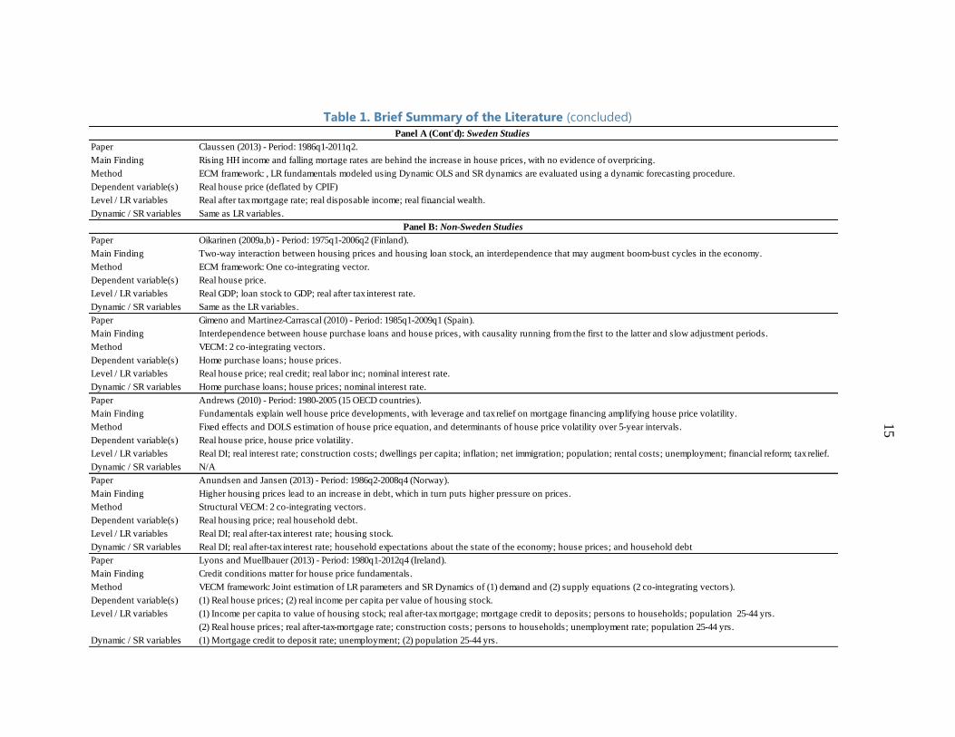
Table 1. Brief Summary of the Literature (concluded)

Paper Claussen (2013) - Period: 1986q1-2011q2.

Main Finding Rising HH income and falling mortage rates are behind the increase in house prices, with no evidence of overpricing.

Method ECM framework: , LR fundamentals modeled using Dynamic OLS and SR dynamics are evaluated using a dynamic forecasting procedure.

Dependent variable(s) Real house price (deflated by CPIF)

Level / LR variables Real after tax mortgage rate; real disposable income; real fi…nancial wealth.


Paper Oikarinen (2009a,b) - Period: 1975q1-2006q2 (Finland).

Main Finding Two-way interaction between housing prices and housing loan stock, an interdependence that may augment boom-bust cycles in the economy.

Method ECM framework: One co-integrating vector.

Dependent variable(s) Real house price.

Level / LR variables Real GDP; loan stock to GDP; real after tax interest rate.

Dynamic / SR variables Same as the LR variables.

Paper Gimeno and Martinez-Carrascal (2010) - Period: 1985q1-2009q1 (Spain).

Main Finding Interdependence between house purchase loans and house prices, with causality running from the first to the latter and slow adjustment periods.

Method VECM: 2 co-integrating vectors.

Dependent variable(s) Home purchase loans; house prices.

Level / LR variables Real house price; real credit; real labor inc; nominal interest rate.

Dynamic / SR variables Home purchase loans; house prices; nominal interest rate.

Paper Andrews (2010) - Period: 1980-2005 (15 OECD countries).

Main Finding Fundamentals explain well house price developments, with leverage and tax relief on mortgage financing amplifying house price volatility.

Method Fixed effects and DOLS estimation of house price equation, and determinants of house price volatility over 5-year intervals.

Dependent variable(s) Real house price, house price volatility.

Level / LR variables Real DI; real interest rate; construction costs; dwellings per capita; inflation; net immigration; population; rental costs; unemployment; financial reform; tax relief.

Dynamic / SR variables N/A

Paper Anundsen and Jansen (2013) - Period: 1986q2-2008q4 (Norway).

Main Finding Higher housing prices lead to an increase in debt, which in turn puts higher pressure on prices.

Method Structural VECM: 2 co-integrating vectors.

Dependent variable(s) Real housing price; real household debt.

Level / LR variables Real DI; real after-tax interest rate; housing stock.

Dynamic / SR variables Real DI; real after-tax interest rate; household expectations about the state of the economy; house prices; and household debt

Paper Lyons and Muellbauer (2013) - Period: 1980q1-2012q4 (Ireland).

Main Finding Credit conditions matter for house price fundamentals.

Method VECM framework: Joint estimation of LR parameters and SR Dynamics of (1) demand and (2) supply equations (2 co-integrating vectors).

Dependent variable(s) (1) Real house prices; (2) real income per capita per value of housing stock.

Level / LR variables (1) Income per capita to value of housing stock; real after-tax mortgage; mortgage credit to deposits; persons to households; population 25-44 yrs.

(2) Real house prices; real after-tax-mortgage rate; construction costs; persons to households; unemployment rate; population 25-44 yrs.

Dynamic / SR variables (1) Mortgage credit to deposit rate; unemployment; (2) population 25-44 yrs.

Panel B: Non-Sweden Studies

Panel A (Cont'd): Sweden Studies

15

16

The role of housing collateral in enhancing households’ ability to borrow has been analyzed in a general equilibrium framework. Aoki, Proudman, and Vlieghe (2004) and Iacoviello (2004, 2005) show that a financial accelerator effect arises in the household sector via house prices, using data for the U.K. and the U.S., respectively. Similarly, Walentin (2014) develops a business cycle model for Sweden that considers the housing sector with variable interest rates on mortgages and a rigid rental market, while accounting for the relatively strict Swedish personal bankruptcy law. In modeling household debt, this paper includes the value of the housing stock to assess the importance of the collateral channel.

Housing supply

Over the medium to longer term, changes in the supply of housing could dampen the impact of demand shocks on prices and also shape the supply of collateral. As housing prices rise relative to construction costs, residential construction becomes more profitable, in time leading to higher supply. In their simulations, Anundsen and Jansen (2013) extend the model of housing prices and household debt to allow for such feedback from housing prices to residential investment. This paper takes a similar approach.

IV. MODELING FRAMEWORK AND DATA

The model presented in this section aims to ensure theoretically sound properties of housing prices and household debt over the long run, while allowing for flexibility in the short-run dynamics for self-reinforcing effects between growth in lending and housing prices along with momentum in housing price growth that could reflect expectations. It comprises three main equations capturing housing prices, household debt, and residential investment.

Housing Prices

The life-cycle model of consumption is the commonly used framework to model housing prices (Meen, 2001; Muellbauer and Murphy, 2008). Similar to other assets, the no-arbitrage value of housing is the discounted value of the future stream of real imputed rental income, with the real user cost of capital as the discount rate.14 The latter is particularly challenging to estimate, being determined by the real after-tax mortgage rate, the risk premium associated with home ownership, property taxes, housing depreciation, expected real house price appreciation, and credit constraints for which a proxy is needed. Since real rental income is unobservable, the housing price equation is rewritten as an inverted demand function (Poterba, 1984). Assuming a log-linear relationship between the variables and adding a stationary error term ε1t, the observed real housing price p can be expressed as a

14 Unlike commercial property, residential housing may not be solely determined by the value of future rents because it provides accommodation to its owners and has thus an intrinsic reservation value.

17

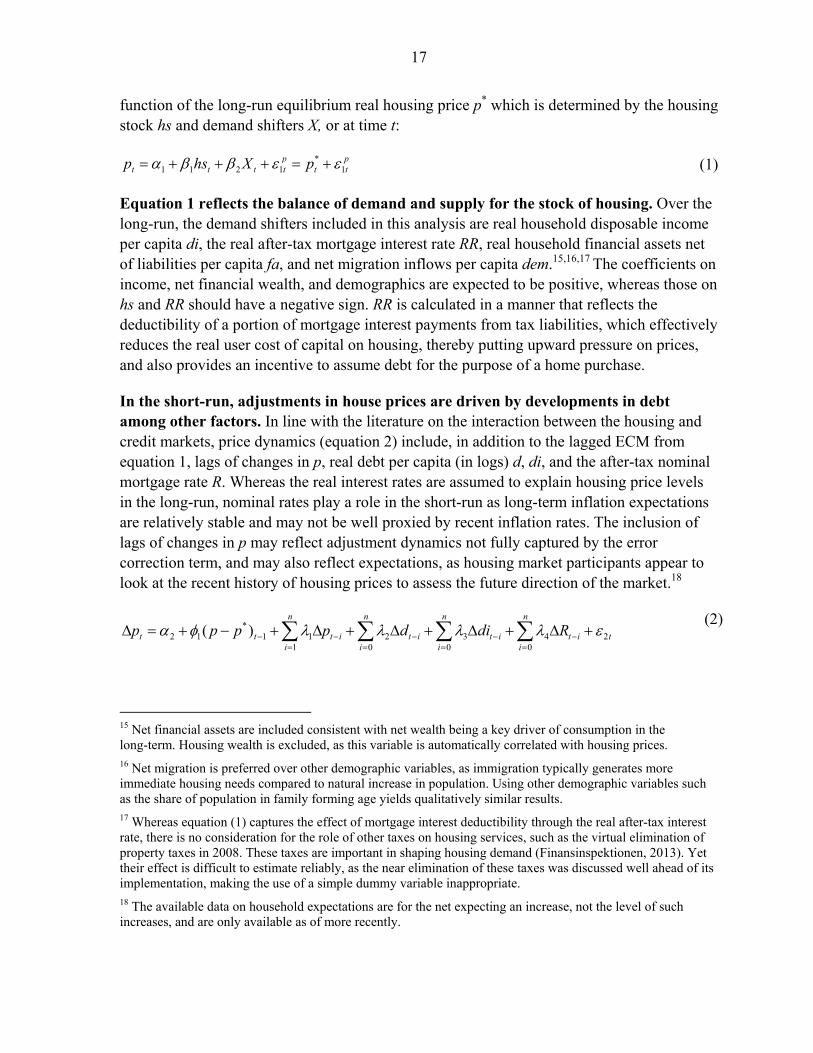
function of the long-run equilibrium real housing price p* which is determined by the housing stock hs and demand shifters X, or at time t:

*1 1 2 1 1

p pt t t t t tp hs X p (1)

Equation 1 reflects the balance of demand and supply for the stock of housing. Over the long-run, the demand shifters included in this analysis are real household disposable income per capita di, the real after-tax mortgage interest rate RR, real household financial assets net of liabilities per capita fa, and net migration inflows per capita dem.15,16,17 The coefficients on income, net financial wealth, and demographics are expected to be positive, whereas those on hs and RR should have a negative sign. RR is calculated in a manner that reflects the deductibility of a portion of mortgage interest payments from tax liabilities, which effectively reduces the real user cost of capital on housing, thereby putting upward pressure on prices, and also provides an incentive to assume debt for the purpose of a home purchase.

In the short-run, adjustments in house prices are driven by developments in debt among other factors. In line with the literature on the interaction between the housing and credit markets, price dynamics (equation 2) include, in addition to the lagged ECM from equation 1, lags of changes in p, real debt per capita (in logs) d, di, and the after-tax nominal mortgage rate R. Whereas the real interest rates are assumed to explain housing price levels in the long-run, nominal rates play a role in the short-run as long-term inflation expectations are relatively stable and may not be well proxied by recent inflation rates. The inclusion of lags of changes in p may reflect adjustment dynamics not fully captured by the error correction term, and may also reflect expectations, as housing market participants appear to look at the recent history of housing prices to assess the future direction of the market.18

*2 1 1 1 2 3 4 2

1 0 0 0

( )n n n n

t t t i t i t i t i ti i i i

p p p p d di R

(2)

15 Net financial assets are included consistent with net wealth being a key driver of consumption in the long-term. Housing wealth is excluded, as this variable is automatically correlated with housing prices. 16 Net migration is preferred over other demographic variables, as immigration typically generates more immediate housing needs compared to natural increase in population. Using other demographic variables such as the share of population in family forming age yields qualitatively similar results. 17 Whereas equation (1) captures the effect of mortgage interest deductibility through the real after-tax interest rate, there is no consideration for the role of other taxes on housing services, such as the virtual elimination of property taxes in 2008. These taxes are important in shaping housing demand (Finansinspektionen, 2013). Yet their effect is difficult to estimate reliably, as the near elimination of these taxes was discussed well ahead of its implementation, making the use of a simple dummy variable inappropriate. 18 The available data on household expectations are for the net expecting an increase, not the level of such increases, and are only available as of more recently.

18

Household Debt

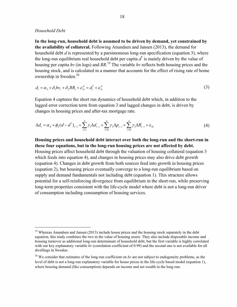
In the long-run, household debt is assumed to be driven by demand, yet constrained by the availability of collateral. Following Anundsen and Jansen (2013), the demand for household debt d is represented by a parsimonious long-run specification (equation 3), where the long-run equilibrium real household debt per capita d* is mainly driven by the value of housing per capita hv (in logs) and RR.19 The variable hv reflects both housing prices and the housing stock, and is calculated in a manner that accounts for the effect of rising rate of home ownership in Sweden.20

*3 1 2 3 3

d dt t t t t td hv RR d (3)

Equation 4 captures the short run dynamics of household debt which, in addition to the lagged error correction term from equation 3 and lagged changes in debt, is driven by changes in housing prices and after-tax mortgage rate.

*4 2 1 1 2 3 4

1 0 0

( )n n n

t t t i t i t i ti i i

d d d d p R

(4)

Housing prices and household debt interact over both the long-run and the short-run in these four equations, but in the long-run housing prices are not affected by debt. Housing prices affect household debt through the valuation of housing collateral (equation 3 which feeds into equation 4), and changes in housing prices may also drive debt growth (equation 4). Changes in debt growth from both sources feed into growth in housing prices (equation 2), but housing prices eventually converge to a long-run equilibrium based on supply and demand fundamentals not including debt (equation 1). This structure allows potential for a self-reinforcing divergence from equilibrium in the short-run, while preserving long-term properties consistent with the life-cycle model where debt is not a long-run driver of consumption including consumption of housing services.

19 Whereas Anundsen and Jansen (2013) include house prices and the housing stock separately in the debt equation, this study combines the two in the value of housing assets. They also include disposable income and housing turnover as additional long-run determinant of household debt, but the first variable is highly correlated with our key explanatory variable hv (correlation coefficient of 0.99) and the second one is not available for all dwellings in Sweden. 20 We consider that estimates of the long-run coefficient on hv are not subject to endogeneity problems, as the level of debt is not a long-run explanatory variable for house prices in the life-cycle based model (equation 1), where housing demand (like consumption) depends on income and net wealth in the long-run.

19

Residential Investment

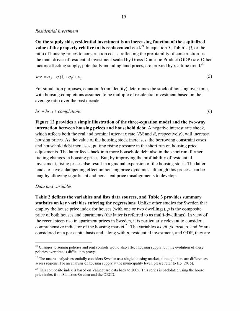
On the supply side, residential investment is an increasing function of the capitalized value of the property relative to its replacement cost.21 In equation 5, Tobin’s Q, or the ratio of housing prices to construction costs--reflecting the profitability of construction--is the main driver of residential investment scaled by Gross Domestic Product (GDP) inv. Other factors affecting supply, potentially including land prices, are proxied by t, a time trend.22

5 1 2 5t t tinv Q t (5)

For simulation purposes, equation 6 (an identity) determines the stock of housing over time, with housing completions assumed to be multiple of residential investment based on the average ratio over the past decade.

hst = hst-1 + completions (6)

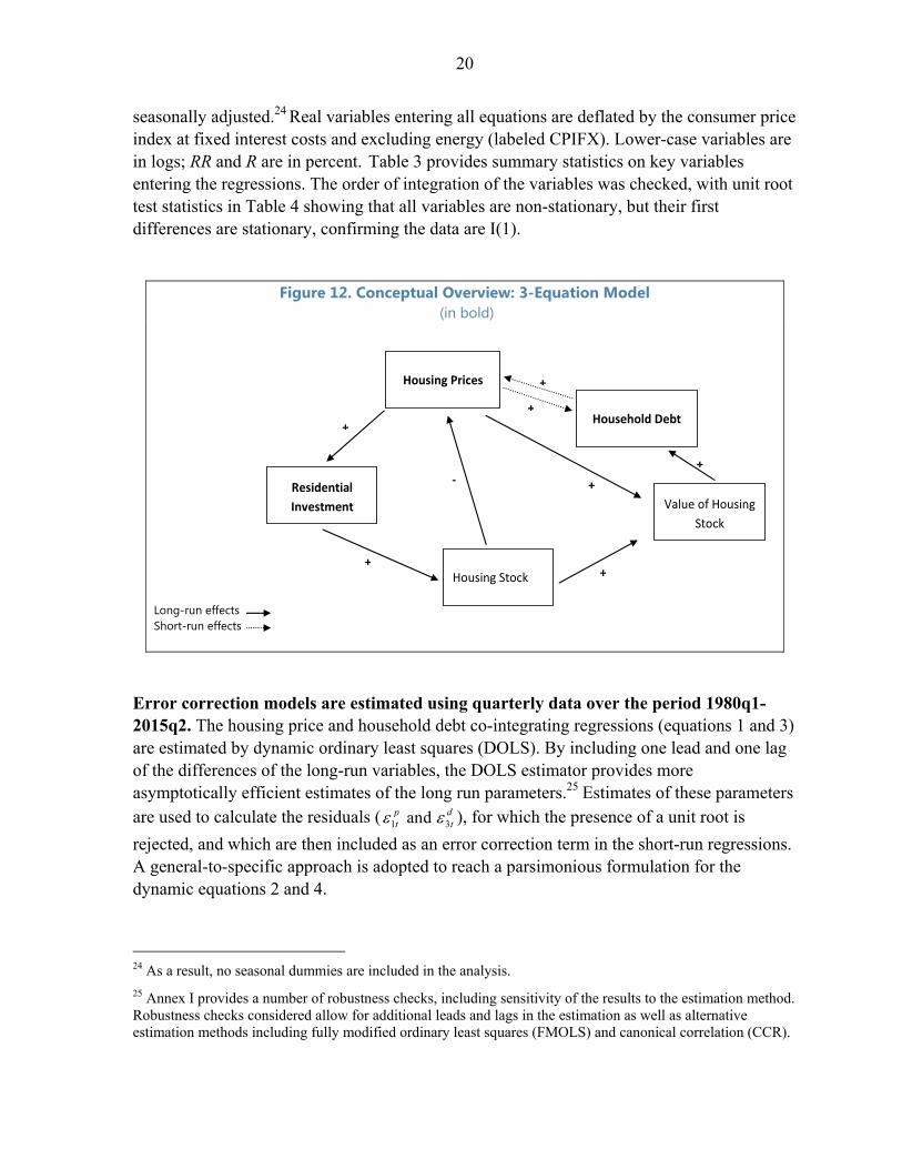
Figure 12 provides a simple illustration of the three-equation model and the two-way interaction between housing prices and household debt. A negative interest rate shock, which affects both the real and nominal after-tax rate (RR and R, respectively), will increase housing prices. As the value of the housing stock increases, the borrowing constraint eases and household debt increases, putting rising pressure in the short run on housing price adjustments. The latter feeds back into more household debt also in the short run, further fueling changes in housing prices. But, by improving the profitability of residential investment, rising prices also result in a gradual expansion of the housing stock. The latter tends to have a dampening effect on housing price dynamics, although this process can be lengthy allowing significant and persistent price misalignments to develop.

Data and variables

Table 2 defines the variables and lists data sources, and Table 3 provides summary statistics on key variables entering the regressions. Unlike other studies for Sweden that employ the house price index for houses (with one or two dwellings), p is the composite price of both houses and apartments (the latter is referred to as multi-dwellings). In view of the recent steep rise in apartment prices in Sweden, it is particularly relevant to consider a comprehensive indicator of the housing market.23 The variables hs, di, fa, dem, d, and hs are considered on a per capita basis and, along with p, residential investment, and GDP, they are

21 Changes to zoning policies and rent controls would also affect housing supply, but the evolution of these policies over time is difficult to proxy. 22 The macro analysis essentially considers Sweden as a single housing market, although there are differences across regions. For an analysis of housing supply at the municipality level, please refer to Ho (2015). 23 This composite index is based on Valueguard data back to 2005. This series is backdated using the house price index from Statistics Sweden and the OECD.

20

seasonally adjusted.24 Real variables entering all equations are deflated by the consumer price index at fixed interest costs and excluding energy (labeled CPIFX). Lower-case variables are in logs; RR and R are in percent. Table 3 provides summary statistics on key variables entering the regressions. The order of integration of the variables was checked, with unit root test statistics in Table 4 showing that all variables are non-stationary, but their first differences are stationary, confirming the data are I(1).

Figure 12. Conceptual Overview: 3-Equation Model

(in bold) Long-run effects Short-run effects

Error correction models are estimated using quarterly data over the period 1980q1-2015q2. The housing price and household debt co-integrating regressions (equations 1 and 3) are estimated by dynamic ordinary least squares (DOLS). By including one lead and one lag of the differences of the long-run variables, the DOLS estimator provides more asymptotically efficient estimates of the long run parameters.25 Estimates of these parameters are used to calculate the residuals ( 1 3and p d

t t ), for which the presence of a unit root is

rejected, and which are then included as an error correction term in the short-run regressions. A general-to-specific approach is adopted to reach a parsimonious formulation for the dynamic equations 2 and 4.

24 As a result, no seasonal dummies are included in the analysis.

25 Annex I provides a number of robustness checks, including sensitivity of the results to the estimation method. Robustness checks considered allow for additional leads and lags in the estimation as well as alternative estimation methods including fully modified ordinary least squares (FMOLS) and canonical correlation (CCR).

+

+

+

+-

++

+

Housing Prices

Household Debt

Value of Housing

Stock

Residential

Investment

Housing Stock

21

Table 2. Variables Definition and Data Sources Variable Source Description

Housing Price, p Valueguard From 2005q1, 2004=100. Backdated to 1986q1 using Statistics Sweden data and to 1980q1 using OECD data. Seasonally adjusted; rebased to 1980q1.

Household Disposable Income, di

Haver From 1980q1. Seasonally adjusted, real, per capita, in logs.

Household Debt, d Haver; Riksbank

From 1996q1 backdated to 1980q1 using data series from the Riksbank on household debt. Series is adjusted for the jump in household debt in 2001q1, assuming that the share of non-loan debt is fixed prior to the series starting in 2001q1. A factor equal to the ratio of Total liabilities to Total Loans from the first quarter where liabilities exceed loans is applied to all data prior to the non-loan debt coming into the series. Seasonally adjusted, real, per capita, in logs.

Housing Value, hv Riksbank; Statistics Sweden

From 1980q1. Cross product of value of household real assets and home tenure. Seasonally adjusted, per capita, in logs.

Household Financial Assets Net of Liabilities, fa

Haver From 1996q1, backdated to 1980q1 using Riksbank’s series on financial assets, with liabilities adjusted for the jump in 2001q1 using the same factor as for the household debt adjustment. Seasonally adjusted, real, per capita, in logs.

After-Tax Mortgage Rate, real RR and nominal R

Riksbank Since 1980q1. In percent.

Housing Stock, hs Statistics Sweden

From 1980q 1. Annual number of dwellings for 1980, 1985, and annual data since 1990. Backdated using quadratic match average and interpolated to quarterly frequency using Statistics Sweden quarterly completions. Per capita, in logs.

Tobin’s Q Statistics Sweden

From 1980q1. Ratio of housing price to construction costs, which is the total factor price index for total dwellings, calculated as a weighted average of construction costs for multi and one-two-dwellings using the share of multi and one-and-two dwellings completions per quarter as weights (1968=100, rebased to 1980q1).

Investment to GDP, inv OECD; Statistics Sweden

From 1980q1. Ratio of residential investment (gross fixed capital formation in housing (buildings and constructions) at constant prices) to GDP (real gross domestic product). Seasonally adjusted, in logs.

CPIFX Statistics Sweden

From 1987q1. Consumer prices at fixed interest costs and excluding energy, backdated to 1980q1 using the KPIX Underlying Inflation measure from Statistics Sweden. In percent.

Population Statistics Sweden

From 1980q1. Annual data interpolated to quarterly frequency using a cubic spline function until 2005, with quarterly data from Statistics Sweden until 2015q1. In thousands.

Net migration, dem Haver From 1980q1. Difference between immigration and emigration flows. Annual data interpolated to quarterly frequency using a cubic spline function. Per capita, in logs.

22

Table 3. Summary Statistics

Variable Obs Mean Max. Min. Std. Dev.

Jarque-Bera Prob.

1st oder autocorr

First difference in real housing prices (Δp) 141 0.01 0.01 -0.08 0.02 0.01 0.51*First difference in real disposable income pc (Δdi) 141 0.00 0.05 -0.05 0.02 0.00 -0.33*First difference in real debt pc (Δd) 141 0.01 0.07 -0.07 0.02 0.00 0.22*First difference in after-tax mortgage rate (ΔR) 141 -0.04 1.94 -1.17 0.44 0.00 0.11

* Significant at the 1 percent level. “D” refers to first difference; pc refers to “per capita”.

Table 4. Unit Root tests. Variable ADF PP KPSS Testing Levels t-ADF 0.05 Adj t-stat 0.050 LM 0.05 Characteristics† p -1.66 -3.45 -2.19 -3.44 0.28 0.15 t

di -2.14 -3.44 -2.75 -3.44 0.24 0.15 t

hs -1.90 -3.45 -3.36 -3.44 0.36 0.15 t

RR -2.49 -3.44 -2.46 -3.44 0.31 0.15 t

fa -3.10 -3.45 -1.99 -3.44 0.13 0.15 t

dem -2.94 -3.44 -2.68 -3.44 0.09 0.15 t

d -1.33 -3.45 -1.24 -3.44 0.26 0.15 t

hv -2.81 -3.45 -2.04 -3.44 0.13 0.15 t Testing first differences p -2.99 -2.88 -7.40 -2.88 0.42 0.46 i di -3.93 -2.88 -16.75 -2.88 0.25 0.46 i hs -2.75 -2.88 -4.79 -2.88 1.07 0.46 i RR -3.57 -2.88 -10.10 -2.88 0.36 0.46 i fa -2.79 -2.88 -9.98 -2.88 0.09 0.46 i dem -4.63 -2.88 -2.61 -2.88 0.05 0.46 i d -3.16 -2.88 -11.61 -2.88 0.23 0.46 i hv -2.72 -2.88 -6.26 -2.88 0.08 0.46 i The null hypothesis for the ADF and PP tests is non-stationarity. By contrast, the KPSS test is based on a null hypothesis of stationarity. † Characteristics include (t) for trend and intercept and (i) for intercept.

23

V. EMPIRICAL FINDINGS

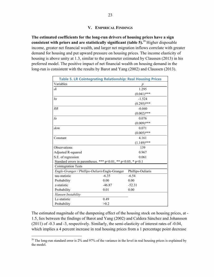
The estimated coefficients for the long-run drivers of housing prices have a sign consistent with priors and are statistically significant (table 5).26 Higher disposable income, greater net financial wealth, and larger net migration inflows correlate with greater demand for housing and put upward pressure on housing prices. The income elasticity of housing is above unity at 1.3, similar to the parameter estimated by Claussen (2013) in his preferred model. The positive impact of net financial wealth on housing demand in the long-run is consistent with the results by Barot and Yang (2002) and Claussen (2013).

Table 5. LR Cointegrating Relationship: Real Housing Prices Variables p

di 1.295 (0.041)***

hs -1.524 (0.295)***

RR -0.040 (0.002)***

fa 0.076 (0.009)***

dem 0.071 (0.005)***

Constant 4.161 (1.149)*** Observations 139 Adjusted R-squared 0.967 S.E. of regression 0.061 Standard errors in parentheses. *** p<0.01, ** p<0.05, * p<0.1 Cointegration Tests

Engle-Granger / Phillips-OuliarisEngle-Granger Phillips-Ouliaris tau-statistic -6.35 -6.54 Probability 0.00 0.00 z-statistic -46.87 -52.31 Probability 0.01 0.00 Hansen Instability Lc-statistic 0.49 Probability >0.2

The estimated magnitude of the dampening effect of the housing stock on housing prices, at -1.5, lies between the findings of Barot and Yang (2002) and Caldera Sánchez and Johansson (2011) of -0.3 and -3, respectively. Similarly, the semi-elasticity of interest rates of -0.04, which implies a 4 percent increase in real housing prices from a 1 percentage point decrease

26 The long-run standard error is 2% and 97% of the variance in the level in real housing prices is explained by the model.

24

in interest rates, is comparable to the findings in the literature summarized in Table 6 (e.g., Hort, 1998; Barot, 2001; Barot and Yang, 2002; Claussen, 2013).

The long-run relationship broadly captures trends in housing prices since 1980. Figure 13 shows that the model tracks well the housing boom and bust in the early part of the sample period, and that trends in predicted housing prices align with actual developments. When the sample estimation period is restricted to 1980q1-2012q4, in-sample prediction for 2013q1-2015q2 shows convergence towards actual housing prices in 2015q2 (figure 14).

Figure 13. Real Housing Prices: Actual vs. Long Run Fitted

(In Logs)

Figure 14. Housing Price Model Predictability (In Logs)

4.05

4.25

4.45

4.65

4.85

5.05

5.25

5.45

1980q3 1986q3 1992q3 1998q3 2004q3 2010q3

Actual

Fitted

Sources: Fund staff estimates

2015q1

3.9

4.1

4.3

4.5

4.7

4.9

5.1

5.3

5.5

1980q1 1986q1 1992q1 1998q1 2004q1 2010q1

Actual HP

Estimation Sample: 1980q1-2013q4

Dynamic Prediction: 2014q1-2015q2

Sources: Fund staff calculations

2015q1

Table 6. Selected Findings from the Literature

Panel A: Sweden Studies Country Interest rate

variable Estimation period

LR Effect of a 1% decrease

in interest rates

SR Effect of a 1% decrease

in interest rates

ECM coefficient

Yearly adjustment

Hort (1998) Sweden Real after-tax mortgage rate

1967-1994 2.9% N/A 0.84 84%

Barot (2001) Sweden Real after-tax LR gvt interest rate

1970h1-1997h2 1.4% 3.3% -0.32 32%

Barot and Yang (2002) Sweden and UK Real after-tax LR gvt interest rate

1970q1-1998q4 2.1% 0.5% -0.12 12%

Adams and Füss (2010) OECD, Sweden included separately

LR interest rate 1975q1-2007q2 0.9% 0.9% -0.04 16%

Caldera Sánchez and Johannson (2011) OECD, Sweden included separately

LR and SR real interest rate

1975q4-2008q4 0.7% 0.0% -0.03 12%

Claussen (2013) Sweden Real after-tax mortgage rate

1986q1-2011q2 6.0% 0.5% -0.08 32%

Turk (2015) Sweden Real after-tax mortgage rate

1980q1-2015q2 4.0% 1.0% -0.08 32%

Panel B: Non-Sweden Studies Country Interest rate

variable Estimation period

LR Effect of a 1% decrease

in interest rates

SR Effect of a 1% decrease

in interest rates

ECM coefficient

Yearly adjustment

Gimeno and Martinez-Carrascal (2010) Spain Nominal interest rate

1984q1-2009q1 3.2% N/A N/A N/A

Lyons, R. and J. Muellbauer (2013) Ireland Nominal mortgage rate

1980q1-2012q4 1.5% 0.5% -0.31 Full

Andrews (2010) OECD panel of countries

Real LR interest rate

1980-2005 0.1% N/A N/A N/A

25

26

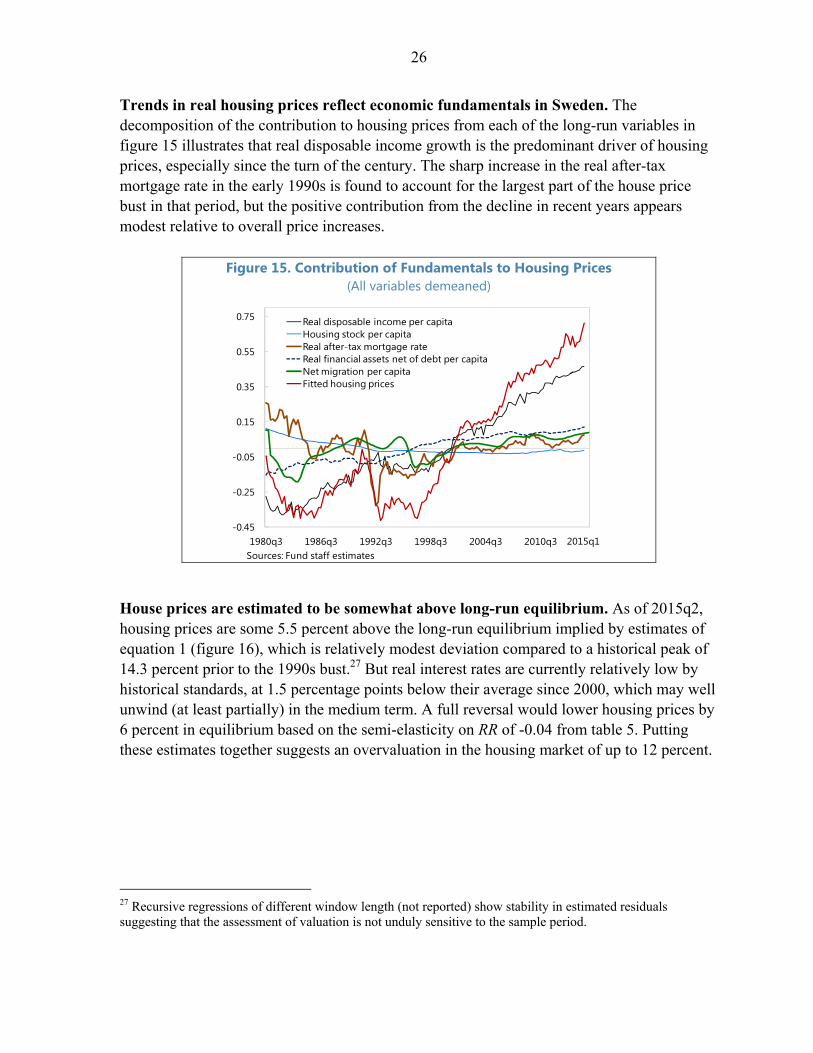
Trends in real housing prices reflect economic fundamentals in Sweden. The decomposition of the contribution to housing prices from each of the long-run variables in figure 15 illustrates that real disposable income growth is the predominant driver of housing prices, especially since the turn of the century. The sharp increase in the real after-tax mortgage rate in the early 1990s is found to account for the largest part of the house price bust in that period, but the positive contribution from the decline in recent years appears modest relative to overall price increases.

Figure 15. Contribution of Fundamentals to Housing Prices (All variables demeaned)

House prices are estimated to be somewhat above long-run equilibrium. As of 2015q2, housing prices are some 5.5 percent above the long-run equilibrium implied by estimates of equation 1 (figure 16), which is relatively modest deviation compared to a historical peak of 14.3 percent prior to the 1990s bust.27 But real interest rates are currently relatively low by historical standards, at 1.5 percentage points below their average since 2000, which may well unwind (at least partially) in the medium term. A full reversal would lower housing prices by 6 percent in equilibrium based on the semi-elasticity on RR of -0.04 from table 5. Putting these estimates together suggests an overvaluation in the housing market of up to 12 percent.

27 Recursive regressions of different window length (not reported) show stability in estimated residuals suggesting that the assessment of valuation is not unduly sensitive to the sample period.

-0.45

-0.25

-0.05

0.15

0.35

0.55

0.75

1980q3 1986q3 1992q3 1998q3 2004q3 2010q3

Real disposable income per capitaHousing stock per capitaReal after-tax mortgage rateReal financial assets net of debt per capitaNet migration per capitaFitted housing prices

Sources: Fund staff estimates2015q1

27

Figure 16. Housing Price Deviation from Fundamentals (In Percent)

Estimates of the short-run dynamics display fairly gradual correction of housing prices toward equilibrium. Table 7 presents the estimation results of equation 2, with statistically insignificant variables eliminated, and standard diagnostic tests not indicating specification issues. The coefficient on the error correction term is negative and significant, pointing to a gradual adjustment in housing prices, correcting around 30 percent of disequilibria over

Table 7. Short-Run Dynamics: Real Housing Prices Δp

ecm-p-1 -0.083 (0.018)***

Δp-1 0.241 (0.079)***

Δp-4 0.262 (0.083)***

Δd-2 0.214 (0.098)**

Δd-3 0.154 (0.085)*

Δdi 0.262 (0.088)***

ΔR-1 -0.010 (0.004)**

Constant 0.001 (0.002)

Observations 137 Adjusted R-squared 0.480 S.E. of regression 0.018 Δ denotes the first difference and Ln refers to the nth lag; where n is omitted L is the first lag. Robust standard errors in parentheses. *** p<0.01, ** p<0.05, * p<0.1

14.3%

-15

-10

-5

0

5

10

15

1980q1 1986q1 1992q1 1998q1 2004q1 2010q1 2015q1

5.5%

28

1 year and about 65 percent over 3 years. As shown in Table 6, the speed of adjustment is similar to Claussen (2013) but faster than OECD estimates for Sweden (Adams and Füss, 2010; Caldera Sánchez and Johansson). As in prior studies, housing price growth shows significant persistence, with lagged coefficients summing to more than 0.5, and disposable income impacts price dynamics contemporaneously well as over time through the error correction term. The second lag of the change in the after-tax mortgage rate serves to accelerate the impact of interest rates on housing prices via the error correction term. Estimates of the short-run equation indicate that debt growth leads housing price adjustments, with effects over some years if not in the long-run. The coefficients in Table 7 on the second (Δd-2) and third (Δd-3) lagged change in household debt are both statistically and economically significant. The sum of these coefficients implies that a 1 percentage point acceleration in lending to households has a first round impact of just under 0.4 percent on housing prices. But this impact is reinforced by the persistence in housing prices mentioned earlier and also by the persistence in debt growth discussed below. The relatively slow adjustment toward equilibrium in both housing prices and household debt means that such dynamic effects may persist for some years.

The upward trend in household debt reflects the rising value of the housing stock owned by households. From table 8, a 1 percent increase in the valuation of housing that is owned by households raises household debt by just under 0.5 percent in the long run, consistent with the role of housing serving as collateral for borrowing.28,29 As housing prices accounted for most of the historical variation in the value of the housing stock, the price of housing was also the main driver of the secular trend in household debt over the long-run.

Declining interest rates also explain the rise in household debt. The semi-elasticity of borrowing to the real after-tax interest rate indicates that a 1 percentage point cut in rates is associated with 3 percent increase in household debt in equilibrium. While no studies from Sweden are available for comparison, Anundsen and Jansen (2013) report similar long-run effects of 1.6 and 2.7 percent in Norway. Allowing for the impact of interest rates on house prices discussed above, the system implies that a 1 percentage point change in interest rates results in a long-run decline in household debt of almost 5 percent—before accounting for the housing supply response.

28 Standard diagnostic tests generally point to cointegration in the variables entering equation 4. 29 Swedish household debt is predominantly in the form of housing loans, representing around 82 percent of total lending to households as of August 2015.

29

Table 8. LR Cointegrating Relationship: Real Household Debt VARIABLES d HH housing value pc 0.470

(0.036)*** Real after-tax rate -0.030

(0.012)** Constant 0.792 (0.416)* Observations 139 Adjusted R-squared 0.950 S.E. of regression 0.084 Standard errors in parentheses. *** p<0.01, ** p<0.05, * p<0.1 Cointegration Tests Engle-Granger / Phillips-Ouliaris Engle-Granger Phillips-Ouliaris

tau-statistic -3.83 -3.55Probability 0.05 0.09

z-statistic -17.78 -14.10Probability 0.18 0.34

Hansen Instability Lc-statistic 0.01Probability >0.2

Housing collateral is the greatest contributor to trends in household debt, and there is mild deviation from fundamentals. The debt model broadly captures trend developments in debt, as illustrated by figure 17. Figure 18 shows that the rising value of the privately owned housing stock explains most increases in household debt, supporting the importance of the collateral channel. The real after-tax interest rate is found to have affected debt most substantially in the 1980s, when inflation was high and the deductible portion of interest payments was higher. The decline in interest rates in recent years makes a rather modest direct contribution to the increase in debt. In terms of debt deviation from long-term trend, figure 19 indicates that it stands at 6.3 percent. Putting this figure in a historical perspective, the misalignment represents about one-third of the peak deviation of 18.5 percent reached in the run-up to the 1990s crisis.

30

Figure 17. Real Household Debt: Actual vs. Long Run Fitted (In Logs)

Figure 18. Contribution of Fundamentals to Household Debt (All variables demeaned)

Figure 19. Household Debt Deviation from Fundamentals (In Percent)

-0.6

-0.4

-0.2

0

0.2

0.4

0.6

0.8

1

1980q3 1986q2 1992q1 1997q4 2003q3 2009q2 2015q1

Actual debt

Fitted debt


-0.8

-0.6

-0.4

-0.2

0

0.2

0.4

0.6

0.8

1980q3 1986q2 1992q1 1997q4 2003q3 2009q2 2015q1

Fitted debt

HH Housing Value

Real After-Tax Mortage Rate


18.5%

-15

-10

-5

0

5

10

15

20

1980Q3 1986Q3 1992Q3 1998Q3 2004Q3 2010Q3


2015q1

6.3%

31

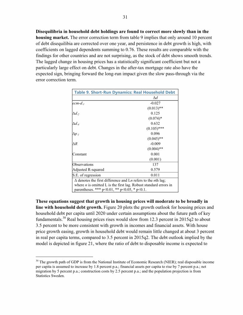
Disequilibria in household debt holdings are found to correct more slowly than in the housing market. The error correction term from table 9 implies that only around 10 percent of debt disequilibia are corrected over one year, and persistence in debt growth is high, with coefficients on lagged dependents summing to 0.76. These results are comparable with the findings for other countries and are not surprising, as the stock of debt shows smooth trends. The lagged change in housing prices has a statistically significant coefficient but not a particularly large effect on debt. Changes in the after-tax mortgage rate also have the expected sign, bringing forward the long-run impact given the slow pass-through via the error correction term.

Table 9. Short-Run Dynamics: Real Household Debt Δd

ecm-d-1 -0.027 (0.013)**

Δd-2 0.125 (0.074)*

Δd-4 0.632 (0.105)***

Δp-1 0.096 (0.045)**

ΔR -0.009 (0.004)**

Constant 0.001 (0.001) Observations 137 Adjusted R-squared 0.579

S.E. of regression 0.011 Δ denotes the first difference and Ln refers to the nth lag; where n is omitted L is the first lag. Robust standard errors in parentheses. *** p<0.01, ** p<0.05, * p<0.1.

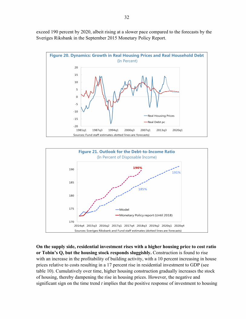
These equations suggest that growth in housing prices will moderate to be broadly in line with household debt growth. Figure 20 plots the growth outlook for housing prices and household debt per capita until 2020 under certain assumptions about the future path of key fundamentals.30 Real housing prices rises would slow from 12.3 percent in 2015q2 to about 3.5 percent to be more consistent with growth in incomes and financial assets. With house price growth easing, growth in household debt would remain little changed at about 3 percent in real per capita terms, compared to 3.5 percent in 2015q2. The debt outlook implied by the model is depicted in figure 21, where the ratio of debt to disposable income is expected to

30 The growth path of GDP is from the National Institute of Economic Research (NIER); real disposable income per capita is assumed to increase by 1.8 percent p.a.; financial assets per capita to rise by 7 percent p.a.; net migration by 5 percent p.a.; construction costs by 2.5 percent p.a.; and the population projection is from Statistics Sweden.

32

exceed 190 percent by 2020, albeit rising at a slower pace compared to the forecasts by the Sveriges Riksbank in the September 2015 Monetary Policy Report.

Figure 20. Dynamics: Growth in Real Housing Prices and Real Household Debt

(In Percent)

Figure 21. Outlook for the Debt-to-Income Ratio (In Percent of Disposable Income)

On the supply side, residential investment rises with a higher housing price to cost ratio or Tobin’s Q, but the housing stock responds sluggishly. Construction is found to rise with an increase in the profitability of building activity, with a 10 percent increasing in house prices relative to costs resulting in a 17 percent rise in residential investment to GDP (see table 10). Cumulatively over time, higher housing construction gradually increases the stock of housing, thereby dampening the rise in housing prices. However, the negative and significant sign on the time trend t implies that the positive response of investment to housing

-20

-15

-10

-5

0

5

10

15

20

1981q1 1987q3 1994q1 2000q3 2007q1 2013q3 2020q1

Real Housing Prices

Real Debt pc

Sources: Fund staff estimates (dotted lines are forecasts)

185%

191%190%

170

175

180

185

190

2014q4 2015q3 2016q2 2017q1 2017q4 2018q3 2019q2 2020q1 2020q4

Model

Monetary Policy report (Until 2018)

Sources: Sveriges Riksbank and Fund staff estimates (dotted lines are forecasts)

33

prices requires increasingly high prices relative to construction costs over time. The time trend could proxy for omitted variables such as land prices, but may also reflect other housing supply constraints. According to Emanuelsson (2015), the decline in state support for financing construction has increased the financial risk of projects which, along with complex land and planning processes at the municipality level and rent controls, may have deterred new construction.

Table 10. Residential Investment VARIABLES Inv Q 0.017 (0.002)*** t -0.016 (0.001)*** Constant 2.396

(0.098)***

Observations 142 Adjusted R-squared 0.766

S.E. of regression 0.2056 Robust standard errors in parentheses. *** p<0.01, ** p<0.05, * p<0.

VI. POLICY ANALYSIS

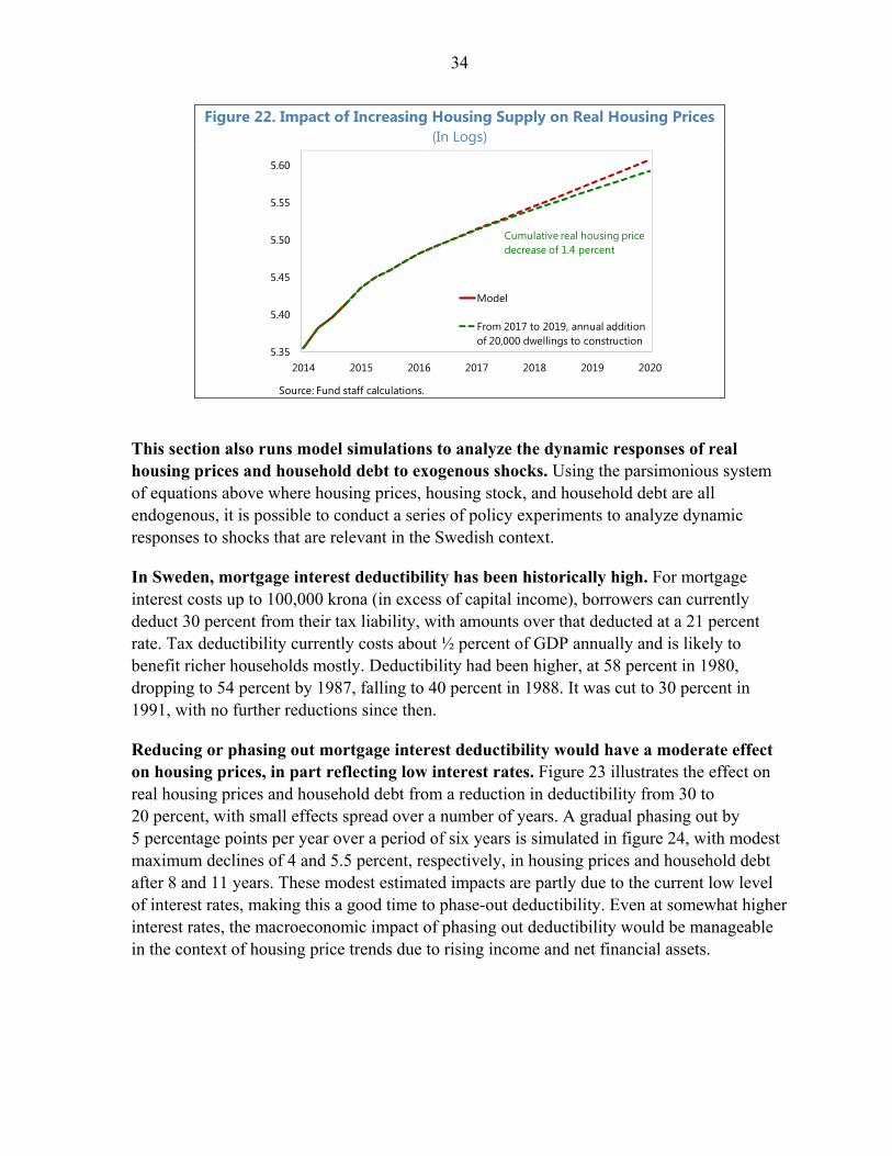
Analysis of government plans to increase the housing stock suggest that their impact on housing prices would likely be small and gradual. The Swedish government announced subsidies for the construction of smaller more affordable rental apartments, with the aim of lifting cumulative dwelling completions to about 250,000 by 2020. Relative to the current baseline outlook for construction, it is assumed that additions to the housing stock will be raised by 20,000 units each year from 2017 to 2019. The impact of such a simulated path, relative to a baseline of no exogenous increase in the housing stock, is depicted in figure 22. Reaching the government’s target implies a 1.3 percent addition to the housing stock, and it is estimated to reduce real housing prices by only 1.4 percent by 2020. Hence, the policy decision to alleviate housing supply constraints is not expected to produce a significant downside to housing prices.

34

Figure 22. Impact of Increasing Housing Supply on Real Housing Prices (In Logs)

This section also runs model simulations to analyze the dynamic responses of real housing prices and household debt to exogenous shocks. Using the parsimonious system of equations above where housing prices, housing stock, and household debt are all endogenous, it is possible to conduct a series of policy experiments to analyze dynamic responses to shocks that are relevant in the Swedish context.

In Sweden, mortgage interest deductibility has been historically high. For mortgage interest costs up to 100,000 krona (in excess of capital income), borrowers can currently deduct 30 percent from their tax liability, with amounts over that deducted at a 21 percent rate. Tax deductibility currently costs about ½ percent of GDP annually and is likely to benefit richer households mostly. Deductibility had been higher, at 58 percent in 1980, dropping to 54 percent by 1987, falling to 40 percent in 1988. It was cut to 30 percent in 1991, with no further reductions since then.

Reducing or phasing out mortgage interest deductibility would have a moderate effect on housing prices, in part reflecting low interest rates. Figure 23 illustrates the effect on real housing prices and household debt from a reduction in deductibility from 30 to 20 percent, with small effects spread over a number of years. A gradual phasing out by 5 percentage points per year over a period of six years is simulated in figure 24, with modest maximum declines of 4 and 5.5 percent, respectively, in housing prices and household debt after 8 and 11 years. These modest estimated impacts are partly due to the current low level of interest rates, making this a good time to phase-out deductibility. Even at somewhat higher interest rates, the macroeconomic impact of phasing out deductibility would be manageable in the context of housing price trends due to rising income and net financial assets.

5.35

5.40

5.45

5.50

5.55

5.60

2014 2015 2016 2017 2018 2019 2020

Model

From 2017 to 2019, annual addition of 20,000 dwellings to construction

Source: Fund staff calculations.

Cumulative real housing price decrease of 1.4 percent

35

Figure 23. Simulation 1: Mortgage Deductibility Reduction from 30 to 20 Percent over 1 Year

Figure 24. Simulation 2: Phasing-Out Mortgage Deductibility by 5 ppts p.a. over 6 years

The last policy experiment seeks to assess the risks from a prolonged period of low interest rates. A prolonged period of low interest rates could arise in case of prolonged weak global growth, leading to more lasting low inflation in Sweden. In an extended period of low interest rates, housing prices and household debt could continue rising. A baseline scenario is for interest rates to remain low for 2 years before normalizing, while this takes 5 years in the shock scenario. Real housing prices and real household debt would increase by 8 and 7 percent more over the 3 years before interest rates begin to normalize, as illustrated by figure 25. This larger misalignment of housing prices and debt could imply greater likelihood of a more difficult adjustment to interest normalization, suggesting advantages to unconventional policies to raise inflation more quickly, and also indicating a heightened need to consider macroprudential measures during a prolonged period of low interest rates that may still be temporary.

-3

-2.5

-2

-1.5

-1

-0.5

0

0 20 30 40 50 60

Impact of Reducing Tax Deductibility on Real Housing Prices(Percent deviation from baseline)


Maximum decrease of 1.4 percent relative to baseline after 4 years

Quarters

-3

-2.5

-2

-1.5

-1

-0.5

0

0 20 30 40 50 60 70 70

Impact of Reducing Tax Deductibility on Real Household Debt(Percent deviation from baseline)


Maximum decrease of 2 percent relative to baseline after 7 years

Quarters

-7

-6

-5

-4

-3

-2

-1

0

0 20 30 40 50 60 70Sources: Fund staff estimates

Maximum decrease of 4 percent relative to baseline after 8 years

Quarters

Impact of Phasing-Out Tax Deductibility on Real Housing Prices(Percent deviation from baseline)

-7

-6

-5

-4

-3

-2

-1

0

0 20 30 40 50 60 70 70Sources: Fund staff estimates

Maximum decrease of 5.5 percent relative to baseline after 11 years

Impact of Phasing-Out Tax Deductibility on Real Household Debt (Percent deviation from baseline)

Quarters

36

Figure 25. Simulation 3: Normalization after a Prolonged Period of Low Interest Rates

VII. CONCLUSIONS AND POLICY IMPLICATIONS

This paper revisits linkages between the housing and household debt markets shedding light on the collateral channel. It explores the drivers of housing prices and household debt, investigates their short-run dynamics, and evaluates potential disequilibria in a low interest rate environment. The findings of modest housing price overvaluation are model-specific and need to be interpreted with caution, and projections suggest a housing price deceleration is more likely that a decline. Although the specification ensures theoretically sound long-run properties, the process of adjustment to equilibrium is gradual, especially for household debt. In that context, there is scope for significant divergences from equilibrium, in part reflecting the dynamic interactions of housing prices and debt. Here, it is notable that the major housing bust in the early 1990s came at a time when housing prices and debt were both significantly above estimated equilibrium levels.

Government policies have played an important role in housing and debt developments and further action may be needed. Government policies to gradually increase housing stock by 2020 are helpful in addressing shortfalls in affordable rental apartments, and are not expected to have significant downside effects on housing prices. Phasing out mortgage interest deductibility is found to help ease demand pressures with a manageable impact on housing prices, and this is associated with a modest decline in household debt. However, a more prolonged period of low real mortgage interest rates is found to increase the potential for more difficult adjustment to a normalization of interest rates, adding to the urgency of returning inflation to the target and also to the considerations underway on macroprudential policy measures including amortization requirements and debt to income ceilings.

-4

-2

0

2

4

6

8

0 20 30 40Sources: Fund staff estimates

Maximum increase of 8 percent relative to baseline after 3 years

Impact of Prolonged Low Interest Rates on Real Housing Prices(Percent deviation from baseline)

Quarters

-4

-2

0

2

4

6

8

0 20 30 40 50 60Sources: Fund staff estimates

Maximum increase of 7 percent relative to baseline after 3 years

Impact of Prolonged Low Interest Rates on Real Household Debt (Percent deviation from baseline)

Quarters

37

References

Adams, Z. and Füss, R. (2010). “Macroeconomic Determinants of International Housing Markets.””Journal of Housing Economics 19(1), pp. 38-50.

Andrews, D. (2010). “Real House Prices in OECD Countries: The Role of Demand Shocks and Structural and Policy Factors”. OECD Economics Department, Working Papers No. 831, OECD Publishing.

Andrews, D., Caldera Sánchez, A. and Johansson, Å. (2011). “Housing markets and structural policies in OECD countries”, OECD Economics Department, Working Paper No. 836. OECD Publishing.

Aoki, K., Proudman, J., and Vlieghe, G. (2004), ‘House Prices, Consumption, and Monetary Policy: A Financial Accelerator Approach’, Journal of Financial Intermediation 13, pp. 414-35.

Anundsen, A. and Jansen, E. (2013). “Self-Reinforcing Effects Between Housing Prices and Credit." Journal of Housing Economics, 22(3), pp.192-212.

Barot, B. and Takala, K. (1998). “House prices and inflation: a cointegration analysis for Finland and Sweden.” Bank of Finland Discussion Papers 12/1998.

Barot, B. (2001). “An Econometric Demand-Supply model for Swedish Housing”. European Journal of Housing Policy 1(3), pp.417-444.

Barot, B. and Yang, Z. (2002). “House Prices and Housing Investment in Sweden and the UK. Econometric analysis for the period 1970-1998.” Review of Urban and Regional Development studies 14(2), pp. 189-216.

Berg, L. and Bergström, R. (1995). “Housing and Financial Wealth, Financial Deregulation and Consumption: The Swedish Case”. The Scandinavian Journal of Economics 97(3), pp. 421-439.

Bernanke, B. and Gertler, M. (1995). ‘Inside the Blackbox: the Credit Channel of Monetary Policy Transmission’, Journal of Economic Perspectives 9(4), pp. 27-48.

Bårdsen, G., den Reijer, A., Jonasson, P., and Nymoen, R. (2012). MOSES: Model for studying the economy of Sweden, Economic Modelling 29, pp. 2566-2582.

Borio, C and Lowe, P. (2002). “Assessing the risk of banking crises.” BIS Quarterly Review, December, pp. 43–54.

Chaney, T., Sraer, D., and Thesmar, D. (2012), “The Collateral Channel: How Real Estate Shocks Affect Corporate Investment”. American Economic Review 102:6, 2381-2409.

38

Caldera Sánchez, A. and Johansson, Å. (2011). “The Price Responsiveness of Housing Supply in OECD Countries”, OECD Economics Department, Working Papers No. 837, OECD Publishing.

Claussen, C. A. (2013). “An Error-Correction Model of Swedish House Prices.” International Journal of Housing Markets and Analysis 6(2), pp. 180 - 196.

Collyns, C. and Senhadji, A. (2002). “Lending booms, real estate bubbles, and the Asian crisis”. IMF Working Paper 02/20. (Washington, D.C.; International Monetary Fund).

Davis, E.P. and Zhum, H.(2011). “Bank lending and commercial property cycles: Some International Evidence.” Journal of International Money and Finance 30, pp. 1-21.

Dennis, J.G., 2006. CATS in RATS, Cointegration Analysis of Time Series, Version 2. Estima: Evanston, Illinois.

Emanuelsson, R. (2015). “Supply of Housing in Sweden.” Sveriges Riksbank Economic Review, 2015:2, pp. 47-75, Sveriges Riksbank, Stockholm, Sweden.

Englund, P., Hendershott, P., and Turner, B. (1995). “The Tax Reform and the Housing Market.” Swedish Economic Policy Review 2, pp. 319-356.

Englund, P. and Ioannides, Y. (1997). “House Price Dynamics: An International Empirical Perspective.” Journal of Housing Economics 6(2), pp. 119-136.

Englund, P. (2015). “The Swedish 1990s banking crisis: A revisit in the light of recent experience.” Paper presented at the Riksbank Macroprudential Conference, Stockholm 23-24 June, 2015.

European Parliament (2013). “Social Housing in the EU”. Directorate General for Internal Policies, Policy Department A: Economic and Scientific Policy, IP/A/EMPL/NT/2012-07, PE 492.469, Brussels.

Finansinspektionen (2013). “Memorandum 1 – Explanations for the Development in Household Debt since the Mid-1990s.” Sten Hansen, Finansinspektionen, Sweden.

Finansinspektionen (2015). “The Swedish Mortgage Market Survey 2015.” April. Finansinspektionen, Sweden.

Finansinspektionen, Riksgälden, and Sveriges Riksbank (2015). The Driving Forces Behind Household Indebtedness in Sweden. Memorandum.

Gerlach, S. and Peng, W. (2005). “Bank lending and property prices in Hong Kong”. Journal of Banking and Finance 29, 461–481.

Gimeno, R. and Martinez-Carrascal, C. (2010). “The Relationship Between House Prices and House Purchase Loans: The Spanish Case.” Journal of Banking and Finance, 34, pp. 1849-55.

39

Greenspan, A., Kennedy, J. (2008). Sources and uses of equity extracted from homes. Oxford Review of Economic Policy 24(1), pp. 120–144.

Ho, G. (2015). “Housing Supply Constraints in Sweden”. Selected issues, Sweden. International Monetary Fund, Washington, D.C.; International Monetary Fund)

Hort, K. (1998). The Determinants of Urban House Price Fluctuations in Sweden 1968-1994. Journal of Housing Economics 7(2), pp. 93.120.

Housing Crisis Committee (2014). “A Functioning Housing Market – A Reform Agenda.” Housing Crisis Committee (Bokriskommittén), Sweden.

Housing Europe (2015). The State of Housing in the EU. The European Federation for Public Cooperative and Social Housing, Brussels.

Hüfner, F. and Lundsgaard, J. (2007). The Swedish Housing Market – Better Allocation via Less Regulation. OECD Economics Department Working Papers, No. 559, OECD Publishing.

Hurst, E. and Stafford, F. (2004). “Home Is Where the Equity Is: Mortgage Refinancing and Household Consumption.” Journal of Money, Credit, and Banking 36(6), pp. 985–1014.

Iacoviello, M. (2004). “Consumption, House Prices and Collateral Constraints: A Structural Econometric Analysis”. Journal of Housing Economics 13, pp. 304–20.

Iacoviello, M. (2005). “House Prices, Borrowing Constraints, and Monetary Policy in the Business Cycle”. American Economic Review 95, pp. 739–64.

International Monetary Fund (2011). Global Financial Stability Report, International Monetary Fund (September), Washington, D.C.

Juselius, K. (2006). The Cointegrated VAR Model: Methodology and Applications. Oxford University Press, Oxford.

Kiyotaki, N. and Moore, J. (1997). ‘Credit Cycles’, Journal of Political Economy 105, pp. 211–248.

Liang, Q., Cao, H. (2007). “Property prices and bank lending in China”. Journal of Asian Economics 18, pp. 63–75.

Lind, H. (2003). “Rent Regulation and New Construction: With a Focus on Sweden 1995-2001. Swedish Economic Policy Review 10, pp. 135-167.

Lustig, H. and van Nieuwerburgh, S. (2005). “Housing Collateral, Consumption Insurance, and Risk Premia: An Empirical Perspective.”Journal of Finance 60(3), pp. 1167–1219.

Lyons, R. and J. Muellbauer (2013). “Explaining the bubble: House prices, user-cost and credit conditions in Ireland, 1975-2012.” Trinity Economics Papers.

40

Meen, G. (2002). “The Time-Series Behavior of House Prices: A Transatlantic Divide?” Journal of Housing Economics 11 (1), pp. 1-23.

Mian, A., Sufi, A. (2011). House prices, home equity-based borrowing, and the US household leverage crisis. American Economic Review 101, pp. 2132–2156.

Muellbauer, J., Murphy, A. (2008). Housing markets and the Economy”. Oxford Review of Economic Policy 24(1), pp.1–33.

Oikarinen (2009a)."Interaction Between Housing Prices and Household Borrowing: The Finnish Case." Journal of Banking and Finance 33, pp. 747–756.

Oikarinen (2009b). “Household Borrowing and Metropolitan Housing Price Dynamics: Empirical Evidence from Helsinki.” Journal of Housing Economics 18 (2), pp. 126–139.

Poterba, J. (1984). “Tax Subsidies to Owner-Occupied Housing: An Asset Market Approach”. Quarterly Journal of Economics 99, pp. 729–752.

Sørensen, P. (2013). The Swedish Housing Market: Trends and Risks. Finanspolitiska rådet. Walentin, K (2014). Housing Collateral and the Monetary Transmission Mechanism.” The Scandinavian Journal of Economics 116(3), pp. 635-668

41

Box 1. Housing Supply and Rent Controls in Sweden

Housing supply shortages in Sweden are large and rising, especially in urban areas. Estimates of housing shortage by the Swedish National Board of Housing, Building and Planning are between 90,000 and 160,000 homes, with around one-third concentrated in Stockholm, and the Stockholm Chamber of Commerce also assesses the deficit to be around 120,000 homes in the Stockholm region (Emanuelsson, 2015). Similarly, the Housing Crisis Committee (2014) evaluates housing shortage at up to 156,000 dwellings, more than half of which are concentrated in the largest three metropolitan areas of Stockholm, Goteborg, and Malmo. According to Housing Europe (2015), up to 276,000 dwellings would be needed to match the increase in population between 2008 and 2013, and it projects the housing shortage to reach 436,000 dwellings by 2020. More recently, the Housing Ministry announced that more than 350,000 young adults are without a home, an increase of 18 percent in two years (Svenska Dagbladet, July 29, 2015).

Another important structural feature of the Swedish model for housing is rent controls. Sweden’s politics reject social housing as segregating and stigmatizing in terms of income and ethnicity. Along with Denmark and the Netherlands, the Swedish model of housing is considered as universalistic aiming to provide the whole population with decent quality housing (European Parliament, 2013). Nevertheless, there is no social housing in Sweden but a complex system of rent controls, making the private rental market the most highly regulated among other OECD countries (Andrews, Caldera Sanchez, and Johansson, 2011).1 According to the Housing Crisis Committee (2014), rent controls have in fact led to the same undesired outcomes as social housing.2

Rent controls keep rent below market levels and result in market rigidity. The benchmark for all rent, including the private sector, comes from rent in the large municipal stock. Municipal housing companies in Sweden own almost half of the rental stock, and they set the norm for market rents following the “tenant’s value system”, with two dwellings having the same characteristics (size, quality, year of construction, and standard) likely to have the same rent. 3 Similar to centralized wage negotiations between labor and employers’ organizations, rent setting has traditionally taken place between the municipal housing companies and representatives from the Swedish Union of Tenants, and it applies to both public and private housing. Despite adding private landlords as a third party to rent negotiations since 2011 and requiring more consideration of the location of the dwelling in annual rent settings, pressure to increase rents has been so far contained by the tenants union, skewing property demand toward older and more attractive dwellings in urban areas. Moreover, lock-in effects from these controls impede mobility and the efficient utilization of the existing rental property.

1 Social housing is present in other countries in Europe, and it is targeted to individuals and households whose demand for housing is not satisfied by the market, as identified by income ceilings or vulnerability. 2 A high number of unemployed people live in the suburbs of the big cities. 3 Public housing in Sweden represents almost 20 percent of the total housing stock and every seventh Swede lives in public housing.

42

ANNEX I. ROBUSTNESS CHECKS

Four major reforms took place in Sweden since the mid 1980s and may have given rise to structural breaks in the system. A tax reform was undertaken in 1983 and 1991 (Englund and Ioannides, 1997); the credit market was deregulated in 1984 (Berg and Bergström, 1995); and there was a change from a fixed to a floating exchange rate in 1992, accompanied by a shift to an explicit inflation targeting monetary policy regime that became operational after 1995. Previous work on the housing market has generally restricted the study period to after 1987, 1992, or 1995, whereas others include a dummy variable post 1992. In this paper, starting the sample from 1980 has the advantage of capturing the decline in the housing market before the boom period in the run-up to the crisis of the 1990s.

Controlling for these structural developments could affect the long-run housing price relationship; yet, sensitivity checks indicate that the main results are qualitatively unchanged. To assess whether the findings are affected by structural breaks, the sample period is reduced to after 1987 (following the first tax reform and financial liberalization in the mid 1980s) and to after the settling of inflation expectations in 1996. The results (not shown but available from the author) indicate that the main findings are maintained. Further, both recursive and reverse recursive estimations are used to assess the stability of the long-run equation, and the results suggest that the long-run relation holds (Dennis, 2006; Juselius, 2006).

The results are also maintained when considering alternative estimation methods for the cointegrating equations. The choice of the DOLS estimator in this paper has the advantage of positioning the results to those in the literature (e.g., Claussen, 2014), but alternative estimation methods are also possible, as shown in tables A1 and A2. In columns 1 to 3, new DOLS specifications include a trend, and two leads and two lags with and without a trend component. Columns 4 and 5 show the results from fully modified ordinary least squares (FMOLS) with and without a trend to estimate the cointegration relationships. Columns 6 and 7 provide the findings from canonical cointegrating regression (CCR) methods in a similar fashion.31 While the parameter estimates are sensitive to the estimation method, the results remain broadly in line with the previous findings.

Additional sensitivity checks do not have a significant effect on the main results. One such test replaces the housing price index used in the analysis with the indicator by the OECD, which has been revised in 2015q2 to add the housing price of multi-dwellings. Other robustness checks consider additional potential economic determinants of household debt such as disposable income, as well as including home tenure separately in equation 3, or lagging Tobin’s Q in equation 5. The findings are qualitatively unaffected.32

31 Whereas the DOLS estimators are obtained by adding leads and lags of the differenced regressors to soak up long-run correlations, FMOLS and CCR eliminate the problems caused by the cross-correlation using a semiparametric correction.

32 The results are available from the author.

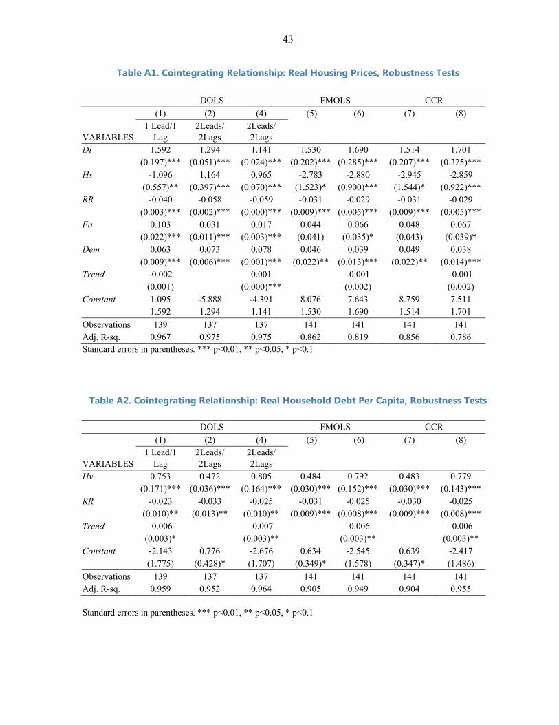
43

Table A1. Cointegrating Relationship: Real Housing Prices, Robustness Tests

DOLS FMOLS CCR

(1) (2) (4) (5) (6) (7) (8)

VARIABLES 1 Lead/1

Lag 2Leads/ 2Lags

2Leads/ 2Lags

Di 1.592 1.294 1.141 1.530 1.690 1.514 1.701 (0.197)*** (0.051)*** (0.024)*** (0.202)*** (0.285)*** (0.207)*** (0.325)***

Hs -1.096 1.164 0.965 -2.783 -2.880 -2.945 -2.859 (0.557)** (0.397)*** (0.070)*** (1.523)* (0.900)*** (1.544)* (0.922)***

RR -0.040 -0.058 -0.059 -0.031 -0.029 -0.031 -0.029 (0.003)*** (0.002)*** (0.000)*** (0.009)*** (0.005)*** (0.009)*** (0.005)***

Fa 0.103 0.031 0.017 0.044 0.066 0.048 0.067 (0.022)*** (0.011)*** (0.003)*** (0.041) (0.035)* (0.043) (0.039)*

Dem 0.063 0.073 0.078 0.046 0.039 0.049 0.038 (0.009)*** (0.006)*** (0.001)*** (0.022)** (0.013)*** (0.022)** (0.014)***

Trend -0.002 0.001 -0.001 -0.001 (0.001) (0.000)*** (0.002) (0.002)

Constant 1.095 -5.888 -4.391 8.076 7.643 8.759 7.511 1.592 1.294 1.141 1.530 1.690 1.514 1.701

Observations 139 137 137 141 141 141 141 Adj. R-sq. 0.967 0.975 0.975 0.862 0.819 0.856 0.786 Standard errors in parentheses. *** p<0.01, ** p<0.05, * p<0.1

Table A2. Cointegrating Relationship: Real Household Debt Per Capita, Robustness Tests

DOLS FMOLS CCR

(1) (2) (4) (5) (6) (7) (8)

VARIABLES 1 Lead/1

Lag 2Leads/ 2Lags

2Leads/ 2Lags

Hv 0.753 0.472 0.805 0.484 0.792 0.483 0.779 (0.171)*** (0.036)*** (0.164)*** (0.030)*** (0.152)*** (0.030)*** (0.143)***

RR -0.023 -0.033 -0.025 -0.031 -0.025 -0.030 -0.025 (0.010)** (0.013)** (0.010)** (0.009)*** (0.008)*** (0.009)*** (0.008)***

Trend -0.006 -0.007 -0.006 -0.006 (0.003)* (0.003)** (0.003)** (0.003)**

Constant -2.143 0.776 -2.676 0.634 -2.545 0.639 -2.417 (1.775) (0.428)* (1.707) (0.349)* (1.578) (0.347)* (1.486)

Observations 139 137 137 141 141 141 141 Adj. R-sq. 0.959 0.952 0.964 0.905 0.949 0.904 0.955 Standard errors in parentheses. *** p<0.01, ** p<0.05, * p<0.1

Housing Price and Household Debt Interactions in … Price and Household Debt Interactions in Sweden...

Documents

Transcript of Housing Price and Household Debt Interactions in … Price and Household Debt Interactions in Sweden...