A Code for Analyzing Coolant and Offgas Activity in a ... Code for Analyzing Coolant and Offgas...
186
A Code for Analyzing Coolant and Offgas Activity in a Light Water Nuclear Reactor: Computer Manual A Code for Analyzing Coolant and Offgas WARNING: Please read the Export Control Agreement on the back cover. Effective December 6, 2006, this report has been made publicly available in accordance with Section 734.3(b)(3) and published in accordance with Section 734.7 of the U.S. Export Administration Regulations. As a result of this publication, this report is subject to only copyright protection and does not require any license agreement from EPRI. This notice supersedes the export control restrictions and any proprietary licensed material notices embedded in the document prior to publication.
Transcript of A Code for Analyzing Coolant and Offgas Activity in a ... Code for Analyzing Coolant and Offgas...

A Code for Analyzing Coolant andOffgas Activity in a Light Water NuclearReactor: Computer Manual
A Code for Analyzing Coolant and Offgas
WARNING:Please read the Export ControlAgreement on the back cover.
Effective December 6, 2006, this report has been made publicly available in accordance with Section 734.3(b)(3) and published in accordance with Section 734.7 of the U.S. Export Administration Regulations. As a result of this publication, this report is subject to only copyright protection and does not require any license agreement from EPRI. This notice supersedes the export control restrictions and any proprietary licensed material notices embedded in the document prior to publication.

CHIRON for WINDOWS – User’sManual
A Code for Analyzing Coolant and Offgas Activity ina Light Water Nuclear Reactor
CM-110056
Computer Manual, June 1998
EPRI Project ManagerB. Cheng
EPRI 3412 Hillview Avenue, Palo Alto, CA 94304, PO Box 10412, Palo Alto, CA 94303, U.S.A. 800.313.3774 or 650.855.2000, www.epri.com

DISCLAIMER OF WARRANTIES AND LIMITATION OF LIABILITIES
THIS REPORT WAS PREPARED BY THE ORGANIZATION(S) NAMED BELOW AS ANACCOUNT OF WORK SPONSORED OR COSPONSORED BY THE ELECTRIC POWERRESEARCH INSTITUTE, INC. (EPRI). NEITHER EPRI, ANY MEMBER OF EPRI, ANYCOSPONSOR, THE ORGANIZATION(S) NAMED BELOW, NOR ANY PERSON ACTINGON BEHALF OF ANY OF THEM:
(A) MAKES ANY WARRANTY OR REPRESENTATION WHATSOEVER, EXPRESS ORIMPLIED, (I) WITH RESPECT TO THE USE OF ANY INFORMATION, APPARATUS,METHOD, PROCESS, OR SIMILAR ITEM DISCLOSED IN THIS REPORT, INCLUDINGMERCHANTABILITY AND FITNESS FOR A PARTICULAR PURPOSE, OR (II) THAT SUCHUSE DOES NOT INFRINGE ON OR INTERFERE WITH PRIVATELY OWNED RIGHTS,INCLUDING ANY PARTY'S INTELLECTUAL PROPERTY, OR (III) THAT THIS REPORT ISSUITABLE TO ANY PARTICULAR USER'S CIRCUMSTANCE; OR
(B) ASSUMES RESPONSIBILITY FOR ANY DAMAGES OR OTHER LIABILITYWHATSOEVER (INCLUDING ANY CONSEQUENTIAL DAMAGES, EVEN IF EPRI OR ANYEPRI REPRESENTATIVE HAS BEEN ADVISED OF THE POSSIBILITY OF SUCHDAMAGES) RESULTING FROM YOUR SELECTION OR USE OF THIS REPORT OR ANYINFORMATION, APPARATUS, METHOD, PROCESS, OR SIMILAR ITEM DISCLOSED INTHIS REPORT.
ORGANIZATION(S) THAT PREPARED THIS REPORT
TransWare Enterprises Inc.
ORDERING INFORMATIONRequests for copies of this report should be directed to the EPRI Distribution Center, 207Coggins Drive, P.O. Box 23205, Pleasant Hill, CA 94523, (510) 934-4212.
Electric Power Research Institute and EPRI are registered service marks of the Electric PowerResearch Institute, Inc. EPRI. POWERING PROGRESS is a service mark of the ElectricPower Research Institute, Inc.
Copyright © 1998 Electric Power Research Institute, Inc. All rights reserved.

iii
CITATIONS
This report was prepared by
TransWare Enterprises, Inc.5450 Thornwood Drive, Suite MSan Jose, California 95123-1222
Principal InvestigatorsK.E. WatkinsB.D. Paulson
This report describes research sponsored by EPRI.
The report is a corporate document that should be cited in the literature in the followingmanner:
CHIRON for WINDOWS—User’s Manual: A Code for Analyzing Coolant and OffgasActivity in a Light Water Reactor, EPRI, Palo Alto, CA: 1998. CM-110056.

iv
v
REPORT SUMMARY
The CHIRON code meets the nuclear industry’s need for a model that can estimate thenumber of failed fuel rods in the nuclear reactor cores of operating BWRs and PWRs.This PC-based tool—now available in WINDOWS format—provides this estimate byusing coolant and/or offgas activity measurements. The WINDOWS version addssignificant flexibility in terms of database capabilities and the code’s use as a generalactivity release management tool. This user’s manual provides a complete tutorial onthe installation and operation of CHIRON as well as its various outputs.
BackgroundThe CHIRON code for coolant and offgas activity data management and analysiscontains three main elements: a database, a sample analysis module, and a trendinganalysis module. The database stores plant design data, cycle operational data, andactivity sample data for multiple cycles along with measurement units and unitconversion information. The database also stores selected analytical results along withmodel parameter settings. The sample analysis module performs a “release-to-birthversus lambda” least squares fit for determining the number of failed fuel rods in thecore. The trending analysis module provides an overview of the variation of a largenumber of measured activities and calculated parameters during a chosen time period.
ObjectivesTo provide a tutorial for the installation and operation of CHIRON and present anoverview of the code’s enhanced capabilities in the WINDOWS version.
ApproachThe project team created a primary user interface featuring enhanced database selectioncapabilities, expanded output options, user-defined plant configuration and modelsettings, options for setting the units of the input data, and open database analysiscapabilities for user-defined plant cycles. The team also increased the ease of editingand printing of plots and analysis reports. Finally, they enhanced CHIRON’s potentialfor handling a larger number of “reactor- soluble” isotopes as well as an expandedseries of isotopic activity expressions. Each of these changes expands the use ofCHIRON as a general activity release management tool. They created this user’s manualto support the enhanced CHIRON WINDOWS version.

vi
ResultsThe CHIRON Main Window is the operating base from where control can be passed toother windows and/or dialog boxes in response to user selections. In specific, CHIRONfeatures
An extensive BWR/PWR failed fuel database A general failure model and a combined failure model specifically developed to
address the low power failure problem, with emphasis on identification of the failedfuel power level
Capabilities for analyzing three groups of fission products, including the noblegases, the iodines, and the reactor solubles
Use of fitted coefficients in conjunction with coolant sample input Calculations that include background activity from tramp fuel and recoil Custom configuration capabilities for individual plants Capabilities for processing a variety of input data and performing single sample and
batch sample analysis Outputs of isotopic ratios as well as outputs conforming to requirements of the
Institute of Nuclear Power Operations (INPO) fuel reliability index Outputs in the form of screen plots and analysis reports for individual samples,
screen plots for trending analysis, and batch export files for transfer of data to aspreadsheet or alternative applications
This user’s manual provides guidance on the installation of CHIRON 3.0, data entrymethods, and the process for converting previous CHIRON databases. It also describesforms of output, structure and contents of the CHIRON database, the theory behindCHIRON calculations, and error message instructions. CHIRON runs on any PC-basedsystem with WINDOWS 3.1 or higher.
EPRI PerspectiveBoth the potential and flexibility of the CHIRON 3.0 WINDOWS version have beensignificantly enhanced relative to previous DOS versions. Use of this version will enableutilities to more accurately assess failed fuel rods on a sample-by-sample or batch basisand produce outputs in a form that will enable them to more effectively manage generalactivity releases and fuel failures.
CM-110056Interest CategoryFuel assembly reliability and performance
KeywordsCHIRON codeLWRFuel rodsFailure analysisActivity release

vii
ABSTRACT
The CHIRON code is a PC based Coolant and Offgas Activity Data Management andAnalysis Tool, now available under WINDOWS. The code contains three mainelements: A database, a sample analysis module, and a trending analysis module. Thedatabase stores plant design data, cycle operational data and activity sample data formultiple cycles, along with measurement units and unit conversion information. Thesample analysis module performs a “Release-to-Birth versus Lambda” least squares fit,from which conclusions are made regarding the number of failed fuel rods in the core.The trending analysis module provides an overview of the variation through a chosentime period of a large number of measured activities and calculated parameters. Aspecial calculation provides the Fuel Reliability Indicator, prescribed by the Institute forNuclear Power Operations. Selected analytical results are also stored in the database,along with the model parameter settings used to produce the analyses. CHIRONaccepts keyboard input on a sample-by-sample basis, or batch input from an ASCII-formatted file. Likewise, sample analysis and database storage can be performed insingle-sample or batch mode. The CHIRON output consists of screen plots and analysisreports for individual samples, screen plots for trending, and batch export files fortransfer of data to a spreadsheet or other alternative application. All plots and text-filereports can be printed, using the available WINDOWS facilities. The potential andflexibility of the CHIRON WINDOWS version have been significantly enhanced relativeto previous DOS versions. The capability of the database to handle units and storemodel parameter settings along with the samples is one example of an enhancement toCHIRON. The ease with which editing and printing of plots and analysis reports can beperformed is another. Furthermore, CHIRON now has the potential to handle a largernumber of “reactor soluble” isotopes, as well as an expanded series of isotopic activityexpressions, which greatly expands the use of CHIRON as a general activity releasemanagement tool.

viii

ix
ACKNOWLEDGMENTS
The CHIRON development was initiated by EPRI in 1987, as a logicalcontinuation of the efforts of the ANS 5.3 Standards Committee. The actualdevelopment of the code was undertaken by S. Levy Incorporated.
We would like to acknowledge the early contributions of Carl Beyer of BattellePacific National Laboratories, who was appointed by the ANS 5.3 StandardsCommittee to compile, sort and analyze the initially collected raw data andadvised the S. Levy Incorporated developers.
Wayne Michaels is also acknowledged for his unwavering commitment to andleadership of CHIRON (MS-DOS version) at S. Levy Incorporated. Forproducing the initial Windows version of CHIRON at S. Levy Inc. we want toacknowledge the efforts of Niels Kjaer-Pedersen and Joe Quintal.
Virginia Jones of TransWare is acknowledged for her efforts in editing theCHIRON 3.0 User Manual.
Last, but not least, we wish to thank EPRI for supporting the enhancements tothe CHIRON Windows version. The EPRI project managers, Rosa Yang, OdelliOzer and Bo Cheng are to be commended for their commitment andencouragement through the various phases of the CHIRON project.

x
xi
TABLE OF CONTENTS
Section Title Page No.
1 INTRODUCTION AND OVERVIEW........................................................................1-11.1 Identification of Problem ..................................................................................1-11.2 Solution Methods.............................................................................................1-11.3 Empirical Failure Modeling ..............................................................................1-21.4 CHIRON Logic Flow ........................................................................................1-21.5 Features and Capabilities ................................................................................1-4
2 GETTING STARTED ..............................................................................................2-12.1 System Requirements .....................................................................................2-12.2 The CHIRON 3.0 Distribution Package............................................................2-12.3 Installing CHIRON from the Diskettes..............................................................2-22.4 Description of the Sample Databases............................................................2-112.5 Running CHIRON 3.0 Tutorial .......................................................................2-12
3 DATA ENTRY.........................................................................................................3-13.1 Data Units (Cardinal Units) ..............................................................................3-13.2 Entering Plant Design and Cycle Operational Data .........................................3-23.3 Entering New Sample Data Input ....................................................................3-8
3.3.1 Single Sample Activity Data Input ..............................................................3-93.3.2 “File Read” (Batch Input) Sample Activity Data Input .................................3-14
4 CHIRON OUTPUT ..................................................................................................4-14.1 Single-Sample Screen Plots ............................................................................4-1
4.1.1 The R/B versus Plot, Offgas and Iodines.................................................4-24.1.2 R/B versus Plot, Solubles ........................................................................4-34.1.3 Cs-Ratio versus Predicted Burnup .............................................................4-54.1.4 f( ) versus Plot .........................................................................................4-6

xii
Section Title Page No.
4.1.5 C( ) versus Plot .......................................................................................4-74.1.6 Failure Correlation Plot...............................................................................4-84.1.7 User Defined X Versus Y Plot ....................................................................4-94.1.8 Editing Single-Sample Screen Plots...........................................................4-9
4.2 Trending Plots .................................................................................................4-94.2.1 Standard Trending Plots...........................................................................4-104.2.2 User Defined Trending Plots ....................................................................4-124.2.3 Editing Trending Plots ..............................................................................4-12
4.3 Screen Reports..............................................................................................4-124.3.1 Offgas Activity Summary Report ..............................................................4-134.3.2 Iodines Activity Summary Report .............................................................4-144.3.3 Solubles Activity Summary Report ...........................................................4-154.3.4 Offgas Release to Birth Summary Report ................................................4-154.3.5 Iodines Release to Birth Summary Report ...............................................4-164.3.6 Solubles Release to Birth Summary Report .............................................4-174.3.7 The Activity Ratio Summary Report .........................................................4-184.3.8 The QA Report .........................................................................................4-194.3.9 The CHIRON Configuration Screen Report..............................................4-19
4.4 Printed Reports..............................................................................................4-194.4.1 The QA Report .........................................................................................4-194.4.2 The Calculation Log Report......................................................................4-194.4.3 The ASCII Dump Files..............................................................................4-19
5 THE CHIRON DATABASE.....................................................................................5-15.1 Database Overview .........................................................................................5-15.2 Database Structure..........................................................................................5-15.3 Creating a New Database................................................................................5-25.4 Compacting a Database ..................................................................................5-35.5 Converting a CHIRON 2.3 Database to CHIRON 3.0......................................5-4

xiii
Section Title Page No.
6 CHIRON THEORY ..................................................................................................6-16.1 FORMULATION OF THE BASIC EQUILIBRIUM EQUATIONS.......................6-1
6.1.1 Least Squares Analysis for Performance Coefficients..............................6-106.1.2 Failure Prediction by the “General Failure Models” ..................................6-156.1.3 Concentration to Release Rate Conversions ...........................................6-20
6.2 COMBINED FAILURE MODEL......................................................................6-266.2.1 Existing Improved Method........................................................................6-266.2.2 Improvement Development for CHIRON..................................................6-276.2.3 Operating Plant Observations ..................................................................6-276.2.4 Data Analysis ...........................................................................................6-286.2.6 Demonstration of Benchmark Fit to Database..........................................6-33
6.3 CHIRON Fuel Failure Database ....................................................................6-376.4 The INPO FRI................................................................................................6-38
7 DIAGNOSTICS AND ERROR CHECKING.............................................................7-17.1 Data Input Error Messages..............................................................................7-17.2 Database Related Error Messages..................................................................7-47.3 Miscellaneous Error Messages........................................................................7-7
8 REFERENCES........................................................................................................8-1
A LIST OF FILES INSTALLED BY CHIRON ............................................................ A-1
B FORMAT OF “FILE READ” ASCII FILE ............................................................... B-1
C SAMPLE QA FILE REPORT ................................................................................. C-1
D ASCII DUMP FILES............................................................................................... D-1D.1 ASCII Dump File “Chirond0.txt” ...................................................................... D-1D.2 ASCII Dump File “Chirond1.txt” ...................................................................... D-2D.3 ASCII Dump File “Chirond2.txt” ...................................................................... D-3D.4 ASCII Dump File “Chirond3.txt” ...................................................................... D-3D.5 ASCII Dump File “Chirond4.txt” ...................................................................... D-4
xiv
Section Title Page No.
D.6 ASCII Dump File “Chirond5.txt” ...................................................................... D-5D.7 ASCII Dump File “Chirond6.txt” ...................................................................... D-6D.8 ASCII Dump File “Chirond7.txt” ...................................................................... D-7D.9 ASCII Dump File “Chirond8.txt” ...................................................................... D-8D.10 ASCII Dump File “Chirond9.txt” ...................................................................... D-9
E CHIRON DATABASE FORMAT............................................................................ E-1

xv
FIGURES
Figure Title Page No.
Figure 1-1 CHIRON 3.0 Logic Flow Diagram ...........................................................1-3Figure 2-1 Welcome to CHIRON 3.0 ........................................................................2-3Figure 2-2 Selecting Installation Type ......................................................................2-4Figure 2-3 The Data Sources List Box Before Registering Databases.....................2-6Figure 2-4 Selecting ODBC Driver ...........................................................................2-7Figure 2-5 Data Source Name Definition Box...........................................................2-7Figure 2-6 Database File Name Selection Box.........................................................2-8Figure 2-7 Registered Database and Driver Designation .........................................2-9Figure 2-8 The Data Sources List Box Showing All Databases Required ..............2-10Figure 2-9 Setup Complete ....................................................................................2-10Figure 2-10 CHIRON Program Group ......................................................................2-11Figure 2-11 CHIRON Main Window .........................................................................2-13Figure 2-12 CHIRON Main Window – Data Drop-Down Menu.................................2-14Figure 2-13 The Data Sources Screen.....................................................................2-14Figure 2-14 Output Options Dialog Box....................................................................2-15Figure 2-15 The Edit Plant-Cycle Configuration Dialog Box.....................................2-16Figure 2-16 The Plant-Cycle Selection Dialog Box...................................................2-17Figure 2-17 Sample Select Dialog Box.....................................................................2-18Figure 2-18 Box Showing Selected Samples ...........................................................2-19Figure 2-19 List of Available Plots ............................................................................2-20Figure 2-20 List of Available Reports .......................................................................2-21Figure 2-21 Dialog Box for Performing Batch Analysis.............................................2-22Figure 2-22 Dialog Box for Trend Plot Selection ......................................................2-22Figure 2-23 Anchor Box for Trend Plotting Control...................................................2-23Figure 2-24 Time-Select Dialog Box.........................................................................2-23Figure 2-25 Trend Plot of Batch Sample Analysis ....................................................2-24Figure 2-26 Trending Graph Customization Dialog Box ...........................................2-27Figure 2-27 Sample Trend Plot ................................................................................2-28

xvi
Figure Title Page No.
Figure 3-1 Edit Units - Sample Data Units................................................................3-2Figure 3-2 Edit Plant-Cycle Configuration Box .........................................................3-3Figure 3-3 Add Plant-Cycle Configuration Box.........................................................3-4Figure 3-4 New Data Dialog Box..............................................................................3-9Figure 3-5 Sample Data Units Dialog Box..............................................................3-10Figure 3-6 Add Sample Data Dialog Box................................................................3-11Figure 3-7 Input File Selection................................................................................3-14Figure 4-1 R/B versus Plot for Offgas and Iodines ................................................4-2Figure 4-2 R/B versus Plot for Solubles ................................................................4-3Figure 4-3 Sample Edit Screen Showing Deletion of Two Cs-Activities ...................4-4Figure 4-4 Revised R/B versus Plot for Solubles...................................................4-4Figure 4-5 Selection of Burnup Model for Cs-Ratio Burnup Prediction.....................4-5Figure 4-6 Cs-Ratio versus Predicted Burnup..........................................................4-6Figure 4-7 f( ) versus Plot......................................................................................4-7Figure 4-8 C( ) versus Plot ....................................................................................4-8Figure 4-9 Failure Correlation Plot for BWRs ...........................................................4-9Figure 4-10 Offgas Activity Summary Report ...........................................................4-14Figure 4-11 Iodines Activity Summary Report ..........................................................4-14Figure 4-12 Solubles Activity Summary Report ........................................................4-15Figure 4-13 Offgas Release to Birth Summary Report .............................................4-16Figure 4-14 Iodines Release to Birth Summary Report ............................................4-17Figure 4-15 Solubles R/B versus Fit Summary Report ..........................................4-18Figure 4-16 Activity Ratio Summary Report .............................................................4-18Figure 5-1 ODBC Access Setup Box........................................................................5-3Figure 5-2 Compact Database Dialog Box ...............................................................5-4Figure 6-1 Combined Failure Model RPF Comparison...........................................6-35Figure 6-2 Combined Failure Model Failure Comparison.......................................6-36Figure 7-1 Sample CHIRON Error Message ............................................................7-1

xvii
TABLES
Table Title Page No.
Table 2-1 Table of Plot Options.............................................................................2-25Table 3-1 Plant Cycle Configuration Data Entry Options ........................................3-5Table 3-2 Sample Data Input Units .......................................................................3-12Table 6-1 Isotopic Decay Data and Fission Yields ..................................................6-2Table 6-2 Calculation of Rod Power Factor and Number of Failures from
Model ....................................................................................................6-33Table E-1 Plant Data Table (plant_data) ................................................................ E-1Table E-2 Sample Data Table (samples)................................................................ E-2Table E-3 Unit Types Data Table (unit_types)........................................................ E-3Table E-4 Units Data Table (units) ......................................................................... E-4Table E-5 User Preferences Data Table (user_preferences) ................................. E-4Table E-6 Failures Data Table (failures)................................................................. E-5


1-1
1 INTRODUCTION AND OVERVIEW
In this section, a brief overview is given of the problem CHIRON attempts tosolve, the means available for the solution, and the approximations that need tobe made to achieve the solution.
An overview of CHIRON’s notable features and capabilities is also provided inthis section. A flow diagram is included to illustrate the main components of theCHIRON program and the path the user will follow when using the code.
1.1 Identification of Problem
In the nuclear industry there is a need for a model that can estimate the numberof failed fuel rods in the nuclear reactor cores of boiling water reactors (BWR)and pressurized water reactors (PWR) during plant operation.
1.2 Solution Methods
CHIRON provides an estimate of the number of failed fuel rods by using coolantand/or offgas activity measurements. The method of analyzing the activitysamples incorporates a theoretical model of the fission product releasecharacteristics of chemically similar nuclides (e.g., iodine nuclides and noble gasnuclides) coupled with an empirical relationship based upon the evaluation ofnumerous release samples from various BWR and PWR reactor cycles.
CHIRON performs a failure analysis with the use of two models: the GeneralFailure Model and the Combined Failure Model. Three groups of fissionproducts are analyzed by CHIRON. These groups include the noble gases, theiodines and the reactor solubles. CHIRON has been prepared to includealternative analyses to handle other subgroups in the future.
The noble gases represent xenon and krypton isotopes for a total of sevenmembers. The noble gases are frequently referred to in CHIRON as “offgas”,because of the method by which measurements are obtained in a BWR. Thisterminology is used herein to refer to PWR noble gas coolant measurements aswell.

Introduction and Overview
1-2
There are five isotopes that represent the iodine group. Activity measurementsof these isotopes are obtained from analysis of coolant samples in both BWRsand PWRs.
The reactor solubles consist of a large number of rather dissimilar isotopicspecies. These isotopes are partly fission products and partly originating fromenvironmental impurities or reactor internals. CHIRON does not provide adirect correlation between the reactor soluble activity measurements and fuelfailures, however, trending of one or more of these nuclides can often be ofbenefit in evaluating and tracking various aspects of fuel performance.
1.3 Empirical Failure Modeling
The General Failure Models are based on empirical fits to the large number ofsamples in the original database. The data used in the failure correlation wasrestricted to reactor power levels above 80 % of rated power, with most of thedata lying near rated power. This is consistent with the fact that most failuresreported during the time span of the database were pellet cladding interaction(PCI) failures, which tend to occur preferentially at substantial power levels.Consistently with these benchmarking conditions, the General Failure Modelshave proven to work quite well for BWRs, for which failures seem to occur morefrequently at medium to high power levels. Unfortunately, the PWR modelshave been somewhat less successful, due to the relatively frequent occurrance oflow power fretting failures. The model improvements for the 1992 versionhelped to alleviate this problem, but the most effective approach to predictinglow power failures is the Combined Failure Model, that has been incorporated inthe current version of CHIRON.
The Combined Failure Model was specifically developed to address the lowpower failure problem. The specific advantage of this model is the identificationof the failed fuel power level. The model is based on the physical observationthat the isotopic diffusion responds differently to temperature changes for offgasand iodines. The difference in isotopic diffusion between offgas and iodinesamples has been correlated to fuel failure data over a wide range of rod powerfor both BWRs and PWRs. The resulting Combined Failure Model providesacceptable fuel failure estimates for rod operating conditions that havetraditionally been difficult to evaluate.
1.4 CHIRON Logic Flow
Figure 1-1 shows a simplified flow diagram of CHIRON. The diagramemphasizes the dataflows, conversions, analyses, and data storage features.

Introduction and Overview
1-3
DB-LIST ODBC
MAIN WINDOW
REGISTERED DATABASESSELECT DATABASES
OUTPUT OPTIONS
PLANT CONFIGURATION AND MODEL SETTINGS
CHOOSECALC. LOG& ASCII DUMP
PLANT CONFIGURATION
MODELPARAMETER SETTINGS
SAVE
OPEN DATA BASE
READ IN NEW DATA
SELECT UNITS
SCREEN INPUT
FILE INPUT
SAMPLE INPUT SCREEN
SELECT PLANT CYCLE(S)
SELECT MULTIPLE SAMPLES
ANALYZE
SAMPLE ANALYSIS RESULTS SCREEN
ASCII DUMP
TREND PLOTS
ANALYZE BATCH
SAVE TO DB
TEXT FILE REPORTS
VIEW
EDIT
SELECT FILENAME FROM LIST
EDIT UNITS
SAVE TO DB
SELECTEDINPUT FILE
PLOTS
SELECT SINGLE SAMPLE
IF ASCII DUMP ENABLED, SPECIFY ASCII DUMP
FILE
EDITSCREEN REPORTS
OTHERWISE
SELECTED DATABASE
Figure 1-1CHIRON 3.0 Logic Flow Diagram
Introduction and Overview
1-4
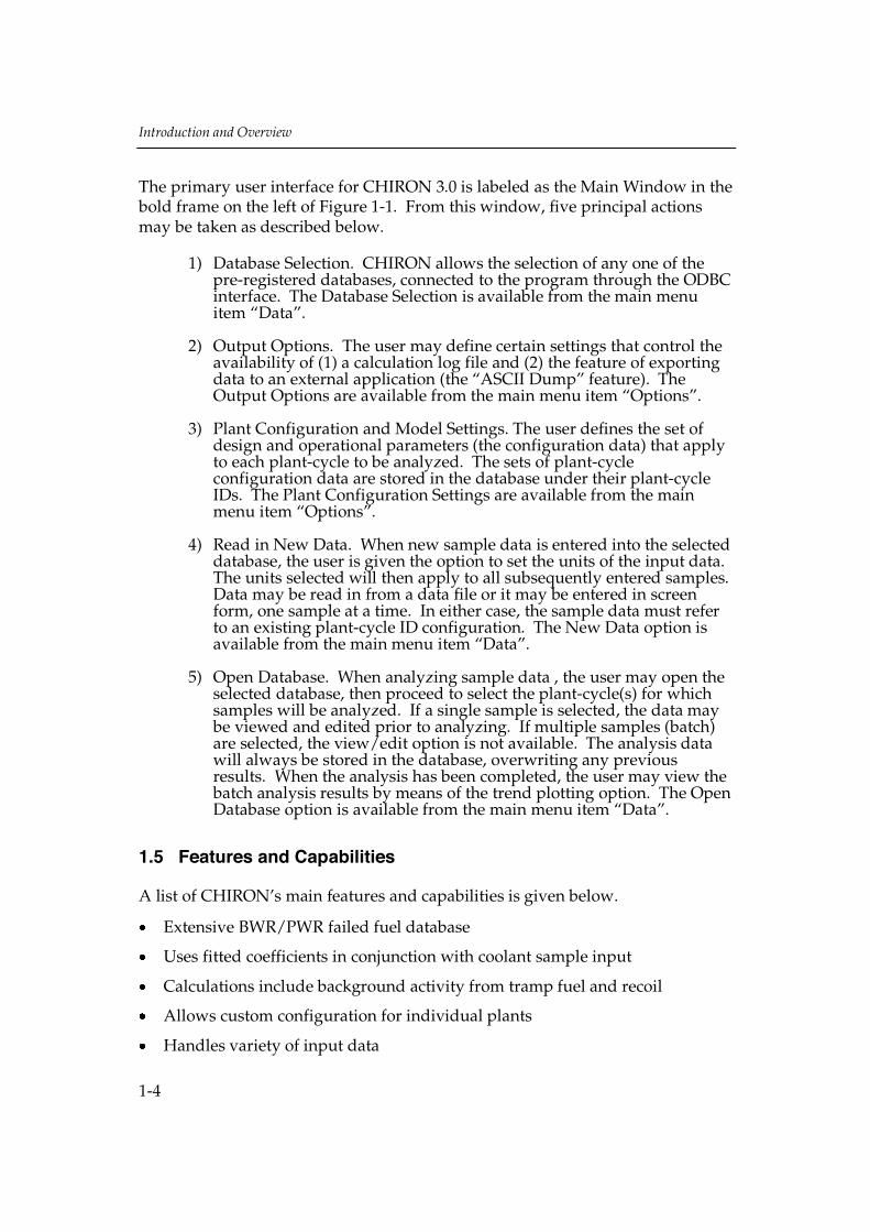
The primary user interface for CHIRON 3.0 is labeled as the Main Window in thebold frame on the left of Figure 1-1. From this window, five principal actionsmay be taken as described below.
1) Database Selection. CHIRON allows the selection of any one of thepre-registered databases, connected to the program through the ODBCinterface. The Database Selection is available from the main menuitem “Data”.
2) Output Options. The user may define certain settings that control theavailability of (1) a calculation log file and (2) the feature of exportingdata to an external application (the “ASCII Dump” feature). TheOutput Options are available from the main menu item “Options”.
3) Plant Configuration and Model Settings. The user defines the set ofdesign and operational parameters (the configuration data) that applyto each plant-cycle to be analyzed. The sets of plant-cycleconfiguration data are stored in the database under their plant-cycleIDs. The Plant Configuration Settings are available from the mainmenu item “Options”.
4) Read in New Data. When new sample data is entered into the selecteddatabase, the user is given the option to set the units of the input data.The units selected will then apply to all subsequently entered samples.Data may be read in from a data file or it may be entered in screenform, one sample at a time. In either case, the sample data must referto an existing plant-cycle ID configuration. The New Data option isavailable from the main menu item “Data”.
5) Open Database. When analyzing sample data , the user may open theselected database, then proceed to select the plant-cycle(s) for whichsamples will be analyzed. If a single sample is selected, the data maybe viewed and edited prior to analyzing. If multiple samples (batch)are selected, the view/edit option is not available. The analysis datawill always be stored in the database, overwriting any previousresults. When the analysis has been completed, the user may view thebatch analysis results by means of the trend plotting option. The OpenDatabase option is available from the main menu item “Data”.
1.5 Features and Capabilities
A list of CHIRON’s main features and capabilities is given below.
Extensive BWR/PWR failed fuel database
Uses fitted coefficients in conjunction with coolant sample input
Calculations include background activity from tramp fuel and recoil
Allows custom configuration for individual plants
Handles variety of input data

Introduction and Overview
1-5
Performs single sample and batch sample analysis
Outputs INPO fuel reliability index
Outputs isotopic ratios
Handles data inputs in numerous unit formats – program converts tostandard units used by program
Generates seven different plots
Generates eight different reports
Plots and reports can be viewed on screen
Ability to print plots for presentation purposes
Printable QA reports
WINDOWS provides the code framework in the form of windows and dialogboxes. The CHIRON Main Window is the operating base from where control canbe passed to other windows and/or dialog boxes in response to the user’sselections. The windows and dialog boxes are largely self-explanatory, but willbe explained in later sections of this manual.
Detailed instructions on the installation of CHIRON 3.0 and a short tutorial areprovided in Section 2 of this manual. The methods used to enter data intoCHIRON are discussed in Section 3. The various forms of output produced byCHIRON are presented in Section 4. The structure and contents of the CHIRONdatabase are described in Section 5. The process for converting previousCHIRON databases is also discussed in Section 5. Section 6 explains the theorybehind the CHIRON calculations. Section 7 provides a list of error messagesgenerated by CHIRON and instructions on what to do if you encounter errormessages. References for this manual are contained in Section 8.
This manual also includes several appendices containing useful information onspecific areas of the CHIRON code. Appendix A lists the files that are installedby CHIRON. Appendix B contains the format for file-read input. Appendix Cshows a sample QA Analysis Report generated by CHIRON. Appendix Dcontains the format of the ASCII dump files that are contained on thedistribution disk. Appendix E contains six tables that list the format of theCHIRON database tables.

Introduction and Overview
1-6

2 GETTING STARTED
2.1 System Requirements
CHIRON is a 16-bit WINDOWS application, developed under WINDOWS 3.1with no use of the Win32s libraries. CHIRON 3.0 for WINDOWS runs underWINDOWS 3.1, WINDOWS 95 and WINDOWS NT operating systems.
The following are the system requirements for installation and efficient use ofCHIRON 3.0 for WINDOWS:
A PC, model 486 or later, with minimum processor speed 50 MHz.
A WINDOWS operating system (3.1x, 95, or NT 4.0).
A VGA monitor or better.
16 MB of RAM.
A hard disk with 15 MB of free space for a “typical” installation.(The exact requirement will be displayed in a separate screen during the“custom” installation.)
A 3.5” floppy drive.
The CHIRON distribution package.
2.2 The CHIRON 3.0 Distribution PackageThe CHIRON Version 3.0 distribution package consists of a set of three 3.5”diskettes, one of which is marked “Disk 1 of 3”. This diskette includes the“Setup” program.
The distribution diskettes include a blank database, “chiblank.mdb”, intended toform the basis for the user in developing his own, plant-specific database. Inaddition, the distribution includes three other databases: “chiron1.mdb”,“chiron2.mdb” and “chiron3.mdb”. These databases all contain test datadesigned to assist the user in getting acquainted with CHIRON and qualifyingthe installation.

Getting Started
2-2
2.3 Installing CHIRON from the DiskettesBefore starting the installation, the diskettes should be backed up and the backupcopies stored in a safe place. Also close all programs on your WINDOWS systembefore starting the installation of CHIRON.
NOTE: These installation instructions are written for a WINDOWS 3.1x user.All illustrations in this manual represent the image one sees if using CHIRON3.0 on WINDOWS 3.1x. For those users on WINDOWS NT or WINDOWS 95,the screens will be the same except for the following: 1) the text in the titlebar will be left justified instead of centered , 2) the symbol used to close awindow and adjust the size of the window are different between WINDOWSapplications. Consult your WINDOWS user manual if you do not know howto close or adjust the window size in your particular application.
Follow the steps below to install CHIRON 3.0 on your computer.
1. Insert Disk #1, into the 3.5” floppy drive. For a WINDOWS 3.1x installation,select “File” from the Program Manager, then select “Run” from the drop-down menu. (For WINDOWS NT or WINDOWS 95, from the “Start” menu,choose Run.) Now, type “a:\setup.exe” into the “Command Line” box, with“a” representing the floppy drive on your computer. Change the “a” if yourfloppy drive is not drive a. Press “Enter” on the keyboard or click “OK” withyour left mouse button.
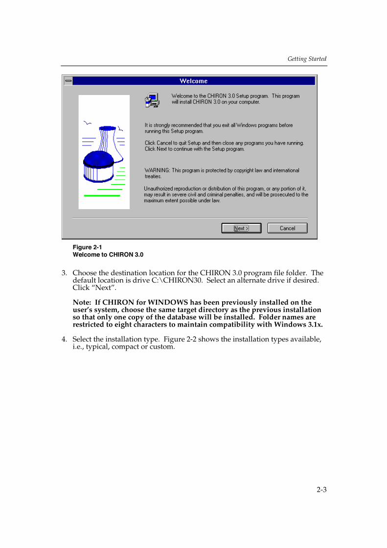
2. The EPRI CHIRON program banner appears and then the first screen (theWelcome screen) of the installation process appears. The Welcome screen isshown in Figure 2-1. Click on “Next” to continue the installation.
Getting Started
2-3
Figure 2-1Welcome to CHIRON 3.0
3. Choose the destination location for the CHIRON 3.0 program file folder. Thedefault location is drive C:\CHIRON30. Select an alternate drive if desired.Click “Next”.
Note: If CHIRON for WINDOWS has been previously installed on theuser’s system, choose the same target directory as the previous installationso that only one copy of the database will be installed. Folder names arerestricted to eight characters to maintain compatibility with Windows 3.1x.
4. Select the installation type. Figure 2-2 shows the installation types available,i.e., typical, compact or custom.

Getting Started
2-4
Figure 2-2Selecting Installation Type
A description of the three types of installation are provided below.
Typical Installation All program files, sample database files,example files, readme files, ODBC drivers, etc.are installed. It is possible to perform a TypicalInstallation on top of an existing installation.The ODBC database registration will beperformed afer the files are installed. Thedatabase registration can be bypassed byimmediately clicking “Close” in the ODBCAdministrator opening box (the ODBC DataSources list box).
Compact Installation Only the program files, database files and thereadme file are transferred. The databasesetup and registration is skipped. Distributiondatabases will be overwritten, but theirregistration will not be affected. This optionmay be useful for installing a new version ofCHIRON, or re-installing the programexecutable if this file were to have beencorrupted by system malfunction.
Getting Started
2-5
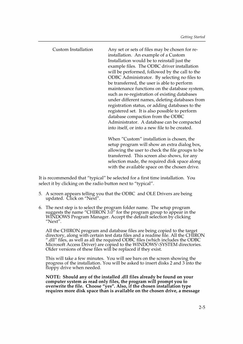
Custom Installation Any set or sets of files may be chosen for re-installation. An example of a CustomInstallation would be to reinstall just theexample files. The ODBC driver installationwill be performed, followed by the call to theODBC Administrator. By selecting no files tobe transferred, the user is able to performmaintenance functions on the database system,such as re-registration of existing databasesunder different names, deleting databases fromregistration status, or adding databases to theregistered set. It is also possible to performdatabase compaction from the ODBCAdministrator. A database can be compactedinto itself, or into a new file to be created.
When ”Custom” installation is chosen, thesetup program will show an extra dialog box,allowing the user to check the file groups to betransferred. This screen also shows, for anyselection made, the required disk space alongwith the available space on the chosen drive.
It is recommended that “typical” be selected for a first time installation. Youselect it by clicking on the radio button next to “typical”.
5. A screen appears telling you that the ODBC and OLE Drivers are beingupdated. Click on “Next”.
6. The next step is to select the program folder name. The setup programsuggests the name “CHIRON 3.0” for the program group to appear in theWINDOWS Program Manager. Accept the default selection by clicking“Next”.
All the CHIRON program and database files are being copied to the targetdirectory, along with certain test data files and a readme file. All the CHIRON“.dll” files, as well as all the required ODBC files (which includes the ODBCMicrosoft Access Driver) are copied to the WINDOWS\SYSTEM directories.Older versions of these files will be replaced if they exist.
This will take a few minutes. You will see bars on the screen showing theprogress of the installation. You will be asked to insert disks 2 and 3 into thefloppy drive when needed.
NOTE: Should any of the installed .dll files already be found on yourcomputer system as read only files, the program will prompt you tooverwrite the file. Choose “yes”. Also, if the chosen installation typerequires more disk space than is available on the chosen drive, a message

Getting Started
2-6
will appear, flagging this condition. If this happens, click on “Cancel” tocancel the installation. A dialog box appears asking if you want to exitSetup. Click “Exit Setup”. Either free space on the target drive or installCHIRON 3.0 on a different drive that has more free space.
7. After copying the files, the setup program automatically installs the ODBCdriver, then opens the ODBC Administrator. At this point, the user mustspecify how the available databases are to be registered. This is done byresponding to a series of dialog boxes in the ODBC Administrator.
A. After an information box, the first dialog box to appear is the DataSources list box as shown in Figure 2-3. During the initial CHIRONinstallation this box will probably be empty. It is possible that you haveother programs on your computer that use ODBC and, therefore, haveexisting registered data sources. Once databases have been registered,the list of registered databases will appear in this box whenever youaccess this dialog box. Now we are going to add a database so click“Add”. This opens the next box.
Figure 2-3The Data Sources List Box Before Registering Databases
B. A list of installed drivers is now displayed as shown in Figure 2-4. Sincethe “Microsoft Access Driver” was installed as part of the CHIRON 3.0installation steps above, it will appear in the list. There may or may notbe other drivers as well, depending on past installations on the computersystem. Select the “Microsoft Access Driver (*.mdb)” by highlighting itand clicking “OK”.

Getting Started
2-7
Figure 2-4Selecting ODBC Driver
C. The next box that appears requests the Data Source Name. Enter“CHIRON DB”. Your screen should look like Figure 2-5. Click “Select”.NOTE: There must always be a valid database that is registered underthe name “CHIRON DB” for CHIRON 3.0 to function properly. This isthe default Data Source name. On starting up, CHIRON will alwayslook for a database registered under this name. After starting theprogram, the user may select any alternative, registered database.
Figure 2-5Data Source Name Definition Box

Getting Started
2-8
D. The Database File Name selection box appears next. Under directories,select the target directory (e.g., C:\CHIRON30). The CHIRON 3.0installation process places four valid database files: “chiblank.mdb”,“chiron1.mdb”, “chiron2.mdb” and “chiron3.mdb” in this directory.Choose the database file “chiron1.mdb” as the Database Name. Yourscreen should look like the one shown in Figure 2-6. Click “OK”. Thistakes you back to the Data Source name selection box. Note that theselected database is now C:\CHIRON30\CHIRON1.MDB, assuming youinstalled in the sample target directory. Click “OK” again.
Figure 2-6Database File Name Selection Box
8. The first database, “chiron1.mdb” has now been registered under the DataSource name “CHIRON DB”, to be used with the “Microsoft Access Driver”.The name “CHIRON DB” appears in the list of registered databases as shownin Figure 2-7.

Getting Started
2-9
Figure 2-7Registered Database and Driver Designation
At this point, it is desirable to add additional databases to the databaseregistry. Choose “Add” and follow steps 7.B. through 7.D. above again toregister the next database, “chiblank.mdb” as Data Source “CHIBLANKDB”, to be used with the “Microsoft Access Driver”. (NOTE: The DataSource name “CHIBLANK DB” is suggested for this exampleinstallation exercise. Any other name compatible with the ODBCconvention may be chosen.) Then, register the remaining two databases“chiron2.mdb” and “chiron3.mdb” as Data Sources “CHIRON2 DB” and“CHIRON3 DB”, respectively, to be used with the “Microsoft AccessDriver”.
Verify that all four data source names now appear as shown in Figure 2-8.Choose “Close” to proceed with the CHIRON installation.

Getting Started
2-10
Figure 2-8The Data Sources List Box Showing All Databases Required
9. The final installation window appears as shown in Figure 2-9 to indicate thatthe setup program is complete. You may be prompted to reboot yourcomputer now. If so, select “Yes”. Click on “Finish” to complete setup. Theinstallation program installs several files on your computer system. For a listof files that are installed, their directory location and purpose, see AppendixA.
Figure 2-9Setup Complete

Getting Started
2-11
10. A program group has been created during the installation that contains fouritems (see Figure 2-10):
The CHIRON 3.0 Program Icon,
The Database Conversion Program Icon,
The Readme File Icon, and
The Uninstall Icon.
The CHIRON Program Icon is used to start the CHIRON program. TheDatabase Conversion Program Icon is used when you want to convertdatabases from older versions of CHIRON. The process for convertingdatabases is explained in Section 5. The Readme File Icon accesses theCHIRON Readme File which contains information which is not found in thisUser Manual and that may apply to a specific application of CHIRON. TheUninstall Icon is used to remove the CHIRON program files from yourcomputer system.
Figure 2-10CHIRON Program Group
2.4 Description of the Sample Databases
Included with the CHIRON 3.0 distribution package are four databases: A blankdatabase, “chiblank.mdb” and three test databases, having filenames
Getting Started
2-12
“chiron1.mdb”, “chiron2.mdb”, and “chiron3.mdb”. The blank database is a pre-formatted CHIRON database, containing all the empty tables that a user needs tocreate his own database. The blank database contains one plant configurationentry, “Plant-nn”. This entry has been included to serve as a template foradditional entries.
The test databases have the following contents:
“chiron1.mdb”: Two BWR cycles, Cycles 5 and 7 of Plant “BWR01”
“chiron2.mdb”: One BWR cycle, Cycle 11 of Plant “BWR02”
“chiron3.mdb”: One PWR cycle, Cycle 9 of Plant “PWR01”
Additional database files may be created by copying any existing database(normally the blank database) to a new filename. See Section 5 for details onhow to create a new database in CHIRON.
2.5 Running CHIRON 3.0 Tutorial
This subsection will provide a sample exercise to familiarize you with some ofthe CHIRON features and show you how to navigate in the CHIRON windows.Follow the steps below to learn how to run CHIRON.
Step 1: Starting CHIRON 3.0
To start CHIRON 3.0, double click on the CHIRON 3.0 for WINDOWS icon in theWINDOWS Program Manager. A CHIRON 3.0 program banner will appearbriefly followed by the main program window as shown in Figure 2-11.

Getting Started
2-13
Figure 2-11CHIRON Main Window
Step 2: Selecting a Database
When CHIRON starts, it automatically opens the database registered under thedefault name “CHIRON DB”. If the installation procedure in Subsection 2.3 hasbeen strictly followed, the selected database is “chiron1.mdb”, containing datafrom BWR01 Cycles 5 and 7.
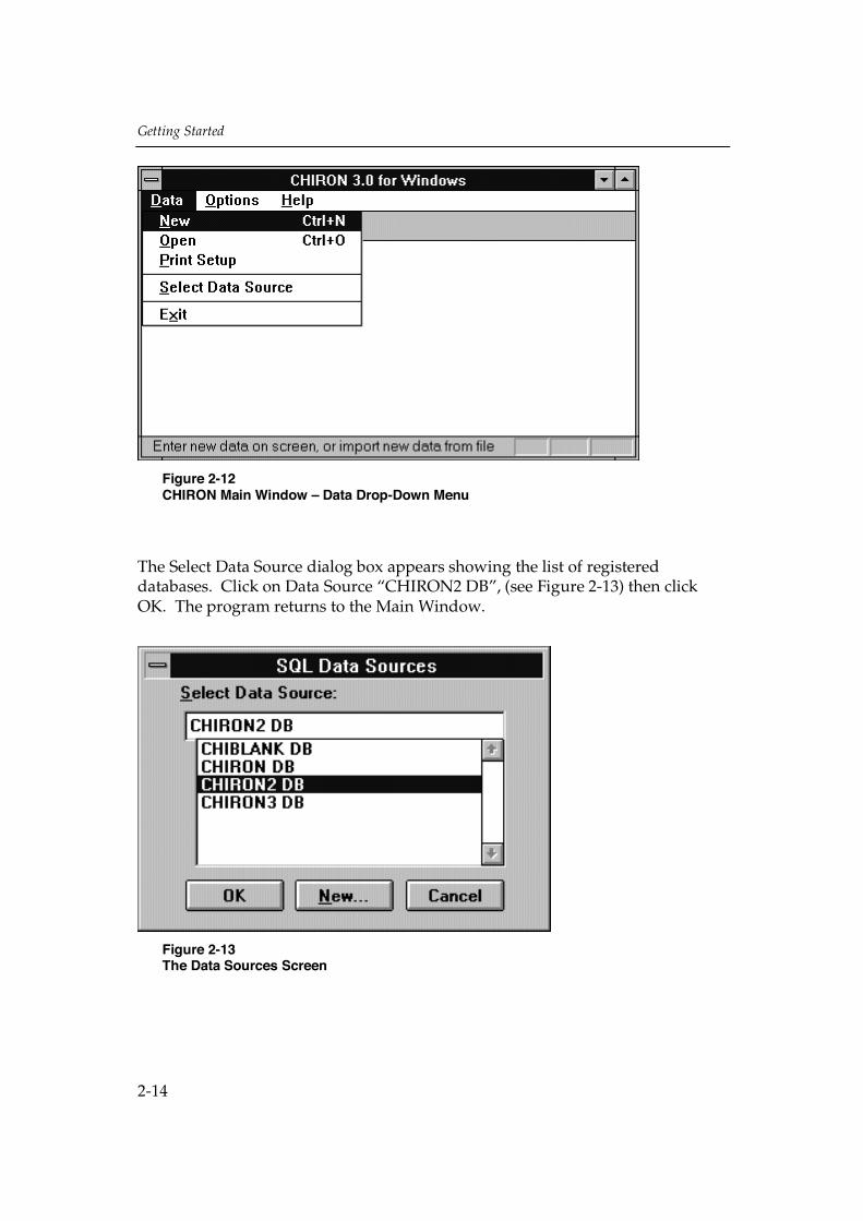
Click on “Data”. The Data drop-down menu appears, see Figure 2-12. Click on“Select Data Source”.
Getting Started
2-14
Figure 2-12CHIRON Main Window – Data Drop-Down Menu
The Select Data Source dialog box appears showing the list of registereddatabases. Click on Data Source “CHIRON2 DB”, (see Figure 2-13) then clickOK. The program returns to the Main Window.
Figure 2-13The Data Sources Screen

Getting Started
2-15
Step 3: Selecting Output Options
From the Main Window select “Options”. Then choose “Output” from the drop-down menu. The dialog box for selecting the output options appears.
In this screen, there are two output options to choose from: 1) a calculation logfile and 2) an ASCII dump file. When selected, the option(s) remains in effectuntil changed during a CHIRON session, or until the program is exited. Youmay select one, both or none of the options from this box.
1. Enable calculation log file for single sample analysis. If you check thisbox, then a text file named “chicalc.log” will be generated at thecompletion of each single sample analysis. The “chicalc.log” file will beplaced in the CHIRON30 folder. This file can be used to retrieve all detailsof the calculational sequence for the last calculated sample. It may be verylarge, on the order of 60 printed pages. This option is not available whenrunning samples in Batch Analysis mode. Once created, the log-file maybe accessed with the use of a text editor. When a new sample analysis isperformed, the previous chicalc.log file is overwritten. The default choicefor this option is no calculation log file.
2. Enable ASCII Dump files for batch analysis. If you check this box, thenASCII dump files will be written and placed in the CHIRON30 folderevery time a batch sample analysis is performed. The default choice forthis option is no ASCII Dump file.
For this exercise, click (check) on both boxes. Your screen should look like theone shown in Figure 2-14. Click OK. The program returns to the main window.
Figure 2-14Output Options Dialog Box

Getting Started
2-16
Step 4: Selecting Plant Cycle Configuration
From the CHIRON 3.0 Main Window, click on Options. Select “PlantConfiguration” from the drop-down menu, then select “Edit Existing Plant”. TheEdit Plant-Cycle Configuration dialog box appears. Select “BWR02-11” from thePlant Cycle ID list in the upper left corner of the box. Notice the data found inthe rest of the box changes to represent the BWR02-11 plant. Now find the placein the lower right section where “Perform Solubles Calculation” is listed as amodel option. Select it by clicking in the box. Your screen should look likeFigure 2-15. Click OK.
Figure 2-15The Edit Plant-Cycle Configuration Dialog Box
Step 5: Select Plant Cycle
Select “Data” from the Main CHIRON 3.0 window, then select “Open”. ThePlant Select dialog box appears as shown in Figure 2-16.

Getting Started
2-17
Figure 2-16The Plant-Cycle Selection Dialog Box
In this dialog box, there is only one plant name, BWR02, available in the list box.Highlight the only available cycle (Cycle 11), then click “Select” (the number 11moves over to the right hand box), then click “OK”.
Step 6: Selecting Samples to Analyze
The dialog box appears as shown in Figure 2-17. As we go through the exerciseusing this box note that there is an extended menu bar at the top containing fournew menu items: Sample, Select, Analysis and Trending. Most of the optionsunder these menu items may be found on the various buttons on this box. Forinstance, the Select menu item contains the “Toggle Status”, “Time-Select Batch”and “Clear All Selections” options. These options also appear as buttons at thebottom of the box. Under the Sample menu, there are a few items that are notfound elsewhere on the box. These items include “Delete Sample”, “DeleteBatch” and “Add Sample”. To use any of these particular options, highlight ormark a sample and then choose the option you desire.
The Sample Select dialog box contains a scrollable list of several hundredsamples. Use the scroll bar on the right side of the table to scroll through the listof samples. Scroll until the top record in the box is as shown in Figure 2-17.

Getting Started
2-18
Figure 2-17Sample Select Dialog Box
Use the mouse to first highlight, then x-mark (by clicking the “Toggle Status”button or by double clicking the mouse button on the sample) the samples dated8/13/95 at time 20:25:00, 8/14/95 at 20:53:00, and 8/15/95 at 21:18:00. Now, usethe mouse to highlight the sample dated 8/12/95, time 20:30:00.
The screen should now look like Figure 2-18. The list shows that the highlightedsample has 6 offgas activities, 5 iodines activities, and 7 solubles activities.

Getting Started
2-19
Figure 2-18Box Showing Selected Samples
Step 7: Performing Single Analysis of Selected Samples
There are two types of analysis that can be performed: 1) Analyze Single or 2)Analyze Batch. Analyze Single analyzes the highlighted sample. Analyze Batchanalyzes the X-marked samples only. For this tutorial, choose “Analyze Single”.The highlighted sample is analyzed. Because the option for “Perform SolublesCalculation” is set, both offgas/iodines and solubles are analyzed. Note: Aninformation message may appear that indicates that the Sum of 6 will be used forthis calculation. Click “OK” to continue.
Step 8: Selecting Plots and Reports
After performing the analysis in Step 7 above, a summary screen report appears.From the menu bar at the top, either “Plots” or “Reports” can now be selected.Figure 2-19 shows the drop-down menu list of types of plots that are available inCHIRON. Click on the various plots to view the result.

Getting Started
2-20
Figure 2-19List of Available Plots
Figure 2-20 shows the drop-down menu list of types of reports that are availablein CHIRON. Click on the various reports to view the generated report. Detaileddescriptions of CHIRON plots and reports are provided in Chapter 4 of thisdocument. Close the Fit Summary Report screen by clicking on OK.

Getting Started
2-21
Figure 2-20List of Available Reports
Step 9: Performing Batch Analysis and Generating ASCII Dump File
The program goes back to the Samples Select box. Click on “Analyze Batch”.You will be asked to enter an ASCII Dump Filename. Click “OK” to accept thedefault filename, “Chirond”. The three samples selected by x-marks will beanalyzed. A box appears as shown in Figure 2-21 showing the status of the batchanalysis including the record being analyzed and the total number that aremarked for analysis. The box also contains a cancel button to stop the analysis.

Getting Started
2-22
Figure 2-21Dialog Box for Performing Batch Analysis
Step 10: Creating Trend Plots
After analyzing the selected samples in Step 9 above, the program opens a dialogbox for trend plot selection as shown in Figure 2-22. This dialog box contains twolist boxes, one for the first y-axis, and one for the second y-axis of a dual y-axistrend plot. Click on the arrow to the right of each box to view the list of choices.Note that the two lists are identical, but default selections are different. A check-box is available to select single y-axis plotting, if desired. It is also possible tocancel trend-plot selection by clicking the “Cancel” button.
Figure 2-22Dialog Box for Trend Plot Selection

Getting Started
2-23
At this point, cancel the trend plot selection by clicking the “Cancel” button (thedefault selection is effective). The program now opens the Trend PlottingAnchor box (see Figure 2-23). This box offers three choices: “DISPLAY TrendGraph”, “SELECT Graph Items” and “Cancel”. Choose “Cancel”. Our presentbatch sample analysis is too small to produce a meaningful trend plot. We willincrease the number of samples so we can produce a more useful trend plot.
Figure 2-23Anchor Box for Trend Plotting Control
After selecting “Cancel”, the program goes back to the Samples Select dialog box(see Figure 2-18). Deselect the previously selected samples by clicking the “ClearAll Selections” button. To get a larger batch selection more suitable for trend-plotting, click on the “Time-Select Batch” button. A dialog box opens to permitthe selection of a time period for batch-analysis/trend-plotting (see Figure 2-24).
Figure 2-24Time-Select Dialog Box

Getting Started
2-24
Enter start date 07/25/95 and end date 08/03/95. Click OK. You are returned tothe Sample Select dialog box. This will select (x-mark) all 36 samples within thistime period. To “thin” the selection, deselect the following samples byhighlighting individually and clicking on the “Toggle Status” button: 7/28/95 attime 23:10:00, 7/29/95 at 21:02:00, 7/30/95 at 20:18:00, 7/31/95 at 21:10:00,8/01/95 at 21:05:00, and 8/02/95 at 20:55:00. Click “Analyze Batch” again. AnASCII dump filename dialog box appears. Then you will see the box showingthe status of the analysis of the samples (similar to Figure 2-21). Next you willsee the trend plot selection screen (Figure 2-22) again.
By default, “Comb. Model Failures” is selected for the Y1 data and “Power” isselected for the Y2 data. The dialog box also allows the selection oflogarithmic/linear scales, as desired, as well as a moving average range (numberof samples over which to average). The moving average can be applied to allfunctions shown in single y-axis plots. Keep the default options, i.e., linear scalesand 7 for running average range. Now press OK. The program returns to theTrend Plot Anchor box. Select “DISPLAY Trend Graph” to display the selectedtrend plot. The plot shown in Figure 2-25 appears.
Figure 2-25Trend Plot of Batch Sample Analysis
Step 11: Customizing Trend Plots
The trend plot appears with the default options for grid-lines, point markers,lines/no-lines, etc. Position your mouse anywhere on the graph. Click the right

Getting Started
2-25
mouse button to bring up the menu for customizing your plot. There are severaloptions available including such things as fonts, grid lines, labels, etc.. Table 2-1below describes these options.
Table 2-1Table of Plot Options
List of Options Description of Function
Viewing Style
Color
Monochrome
Monochrome + Symbols
Choose the way you want your plot displayed.
Plot will be displayed in color.
Plot will be displayed in monochrome.
Plot will be displayed in monchrome + symbols.
Font Size
Large
Medium
Small
Choose the font size you want used in your plotheadings and data.
Use large size fonts.
Use medium size fonts.
Use small size fonts.
Numeric Precision
No Decimals
1 Decimal
2 Decimals
3 Decimals
Choose the numeric precision to be used in plottingthe data points.
Integer numbers used when plotting data points.
Numbers truncated to one decimal point in plots.
Numbers truncated to two decimal points in plots.
Numbers truncated to three decimal points in plots.
Data Shadows Places a shadow on each data point to increasevisibility.
Grid Lines
Both Y and X Axis
Y Axis
X Axis
No Grid
Show grid lines on plot display.
Show grid lines on both axes.
Show grid lines on the Y Axis only.
Show grid lines on the X Axis only.
Do not show grid lines on the plot display.
Grid in Front Grid lines appear in front of data points. If a datapoint falls directly on a grid line, the data point isobscured.

Getting Started
2-26
List of Options Description of Function
Include Data Labels Unique identifying labels are placed on each datapoint. Some plots have data labels designedspecifically for that plot, while others will showdefault numeric, sequential data labels.
Mark Data Points Put dots to mark the data points on the plot. Bydefault this option is selected.
Show Annotations Annotations have been set for certain plots. Ifannotations are set, they will appear when this isselected. The user cannot make customizedannotations. By default this option is selected.
Undo Zoom Display the plot in normal scale.
Maximize Maximize the size of the plot display.
Customization Dialog
General
Plot Style
Subsets
Fonts
Color
You can edit the various style settings to customizeyour plot display. Many of the items found in thisoption are available as individual options elsewherein this menu, but are repeated here on one menu toallow you to customize everything at once. Thereare many plot styles to choose from such as bar,area, line, points, etc. See the Help option forassistance on using all of these options.
Export Dialog
Export:
Metafile
Bitmap
Embedded Object
Text/Data Only
Export To:
Clipboard
File
Printer
Export the plot. Determine the file type forexporting, the destination for the export and theobject size for exporting.Export the plot in metafile format.
Export the plot in bitmap format.
Export the plot in embedded object format.
Export the plot in text/data file format.
Export the plot to the clipboard.
Export the plot to a file.
Export the plot to a printer. Choose the size toprint, i.e., full-size or a specified size.
Help Displays help screen containing a indexed list ofhelp categories for the options found on this menu.Find the option you need help with and a detailedexplanation will be provided on the use of theoption.

Getting Started
2-27
To see an example of a couple of these features, start by choosing “Grid Lines”from the menu. This brings up a submenu. Click on “Both Y and X Axis”. Theplot reappears with gridlines. Now, click the right mouse button again andchoose the “Customization Dialog”. A dialog box appears that has five sheets:General, Plot Style, Subsets, Font, and Color. Choose the sheet named “PlotStyle”. You will see the screen shown in Figure 2-26.
Figure 2-26Trending Graph Customization Dialog Box
From that sheet, under “Axes”, choose the y-axis labeled “Comb. ModelFailures”. Under “Plot Style” select “Line”. Next, select another choice under“Axes”, “Power Frac Pwr”. Select “Line” for Plot Style again. Accept the changesby clicking “Apply”. To show your action has been applied, the “apply” buttonis grayed or disabled now. Then click OK to get back to the plot. The plot hasnow changed its appearance as shown in Figure 2-27. Experiment some more tobecome familiar with the various options for customizing your plots.

Getting Started
2-28
Figure 2-27Sample Trend Plot
Two additional features are found in the trend plots and are accessed with themouse button. As you move the mouse button on the plot note there is a timeand number shown on the upper left corner of the plot. As you move the mouse,the number changes. This number identifies the coordinates of the mouse cursorwithin the graph area. If you leave the graph area, the number disappears. Alsonote that when the mouse is directly on a data point on the graph, a tiny handappears so you know you are on a data point and can identify the coordinatesshown in the upper left corner with that point. Put your mouse directly on adata point and see the tiny hand symbol.
A second feature that is useful when working with plots, is the zoom feature. Tozoom in (magnify) on a particular portion of the plot, click and hold down themouse button while moving the mouse over the area you wish to enlarge. A boxwill form on the screen indicating the area you are encompassing in your zoom.When you release the mouse button you see part of the plot in an enlarged state.When you wish to return to the normal plot state, click on the right mouse buttonand select the “undo zoom” option.

Getting Started
2-29
Step 12: PrintingFinally, as a final exercise in trend plots, try printing to an available WINDOWSprinter by performing the following: from the right mouse button menu, choosethe “Export Dialog”. From the Export Dialog choose “MetaFile” as the type offile you are exporting; “Printer” as the export designation; and “Full Page” asobject size. Click “Print”. A printer configuration box appears. Verify theprinter you are printing to, the paper selection, etc. Click OK. If an appropriateprinter configuration exists under WINDOWS, the plot will be printed.
Step 13: Exiting from CHIRON
Now, close the trend plot by pressing the “Esc” key on the keyboard. The anchorbox reappears. Press “Cancel” to quit trend plotting. On “Cancel”, the programgoes back to the Samples Select dialog box (Figure 2-18). Close this box. Theprogram goes back to the main window. Select “Exit” under the “Data” menu toexit from CHIRON.

Getting Started
2-30

3-1
3 DATA ENTRY
This section provides detailed information on the various methods and formatsused to enter new data and edit existing data in the CHIRON 3.0 database. Twomethods of entering new data are supported in CHIRON: screen input and fileinput. All data entered into the CHIRON 3.0 database must conform to thedatabase structure and data units. Data units, data ranges and default values (ifavailable) for each data type are provided in this section. CHIRON allows theuser to input the numerical values in any numerical format, i.e., decimal, integer,or exponential.
A data range checking procedure in CHIRON 3.0 performs unit conversionswhere appropriate. It also performs certain checks on input data to minimize therisk of serious numerical problems due to accidentally entered input values thatare dramatically out of range. Tables 3-1 and 3-2 list the acceptable CHIRON dataranges.
3.1 Data Units (Cardinal Units)
When data is input to CHIRON the user must be sure to use the data units thatare supported by the CHIRON program. Units are defined in the CHIRONdatabase for each data entry field. A set of reference units, referred to as the“Cardinal Units” are used internally in CHIRON, as well as for all on-screenoutput. In addition, the user selects a set of input units from a pre-defined list ofchoices shown in list-boxes on the sample data units screen.
To check the data units currently in effect, perform the following:
From the main window, select “Data”
Click on “New”
Select “Edit Units” from the New Data dialog box. The Sample Data Unitsdialog box appears and lists the Cardinal Units for each sample data inputitem (see Figure 3-1).

Data Entry
3-2
Figure 3-1Edit Units – Sample Data Units
The asterisks in parentheses indicate that these are cardinal units that CHIRONuses internally. CHIRON converts from the selected units to the appropriatecardinal units, using built-in conversion factors.
Note: CHIRON initially has the cardinal units set as the selected units. Aschanges are made to the input units, the selections are saved in the database.Therefore, the latest choice made will be in force until changed by the user.
3.2 Entering Plant Design and Cycle Operational Data
Prior to entry of new sample data, the user needs to check that the Plant-Cycle IDexists in the database. This is done by clicking on “Options” from the MainWindow, followed by “Plant Config”, then selecting “Edit Existing Plant”. Thisopens the Edit Plant-Cycle Configuration Box as shown in Figure 3-2.
Data Entry
3-3
Figure 3-2Edit Plant Cycle Configuration Box
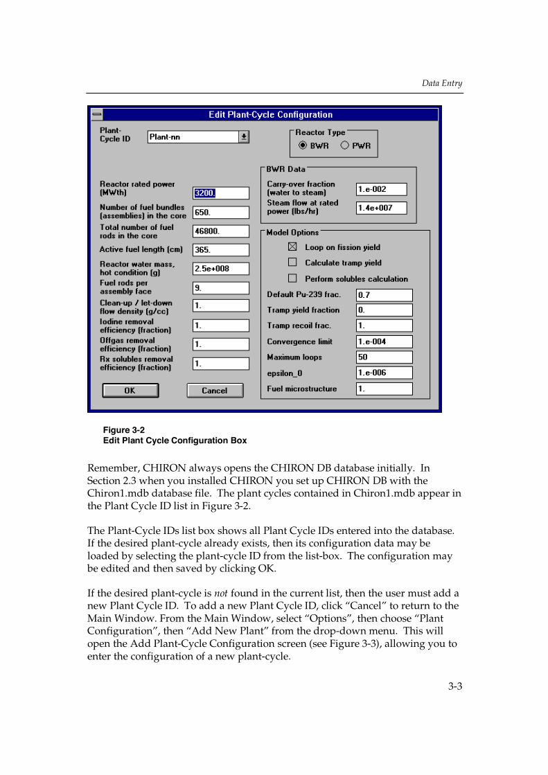
Remember, CHIRON always opens the CHIRON DB database initially. InSection 2.3 when you installed CHIRON you set up CHIRON DB with theChiron1.mdb database file. The plant cycles contained in Chiron1.mdb appear inthe Plant Cycle ID list in Figure 3-2.
The Plant-Cycle IDs list box shows all Plant Cycle IDs entered into the database.If the desired plant-cycle already exists, then its configuration data may beloaded by selecting the plant-cycle ID from the list-box. The configuration maybe edited and then saved by clicking OK.
If the desired plant-cycle is not found in the current list, then the user must add anew Plant Cycle ID. To add a new Plant Cycle ID, click “Cancel” to return to theMain Window. From the Main Window, select “Options”, then choose “PlantConfiguration”, then “Add New Plant” from the drop-down menu. This willopen the Add Plant-Cycle Configuration screen (see Figure 3-3), allowing you toenter the configuration of a new plant-cycle.

Data Entry
3-4
Figure 3-3Add Plant-Cycle Configuration Box
Add the data in each box starting with Reactor rated power. Click on the datafield you are entering and type in the appropriate data. Be sure to enter thedata in the units noted in parentheses next to the item, i.e., Reactor rated powermust be entered in MWth units. Table 3-1 provides detail on the Plant CycleConfiguration data entries, including the acceptable data ranges and any defaultvalues used in the program. Note: Unless otherwise indicated, data valuesmay be entered in any numeric format, i.e., decimal, integer or exponential.The program will convert the entries to the Cardinal Units used internally bythe program.
When you click OK, the program performs a range check on each value. If allvalues are acceptable, then the data is saved to the database and you are returnedto the CHIRON main window. If you click on the “Cancel” button, then the datais not saved and you are returned to the CHIRON main window.

Data Entry
3-5
If any data item is out of range, a message will appear showing a list of all itemsthat are out of range. On clicking OK, the user is returned to the dialog box to fixthe problem(s). No data will be entered into the database until all the requiredranges have been satisfied.
Table 3-1.Plant Cycle Configuration Data Entry Options
Plant Cycle Config. Data Data Range Description
Reactor rated power 0<RatPow 10000 in MWth
The reactor rated power.
No. of fuel assemblies inthe core
0<NFAss 2000
in any numericformat
The number of fuel assemblies in thereactor core.
Total number of fuel rodsin the core
n2 * NFAss * 0.5
Nrods n2 *NFAss * 2
The total number of fuel rods in thereactor core.
Active fuel length 0<Act FuelL
1000 in cm
The length of the active fuel.
Reactor water mass, hotcondition
1.0x10⁵ WM
1.0x10¹⁰ in grams
The water mass in the reactor at hotcondition.
Fuel rods per assemblyface
For BWRs:
6 n 12
ForPWRs:14 n 20
The number of fuel rods per assemblyface.

Data Entry
3-6
Plant Cycle Config. Data Data Range Description
Clean-up/let down flowdensity
0.5 CUDens 2.0in g/cc
The cleanup or letdown flow density.
Iodine removal efficiency 0<IEff 1 infraction
The Iodine removal efficiency (normallyassumed to be unity) is used to computethe isotopic loss term caused by the clean-up/letdown system. This valuerepresents the efficiency of the removalsystem (e.g. the ion-exchange beds). Thisvalue may vary slightly over time, butshould remain very close to 1.0representing 100% removal efficiency.
Offgas removal efficiency 0<OGEff 1
in fraction
The Offgas removal efficiency (normallyassumed to be unity) is used to computethe isotopic loss term caused by the clean-up/letdown system. This valuerepresents the offgas removal efficiencyof the letdown flow system. This valuemay vary slightly over time, but shouldremain very close to 1.0 representing100% removal efficiency.
Rx solubles removalefficiency
0<RxEff 1
in fraction
The Rx solubles removal efficiency(normally assumed to be unity) is used tocompute the isotopic loss term caused bythe clean-up/letdown system. This valuerepresents the efficiency of the removalsystem (e.g. the ion-exchange beds). Thisvalue may vary slightly over time, butshould remain very close to 1.0representing 100% removal efficiency.

Data Entry
3-7
Plant Cycle Config. Data Data Range Description
Loop on fission yield If this option is selected, CHIRONperforms an iteration on the Pu239 fissionyield ratio for the failed fuel. CHIRONsearches for the fission yield thatprovides the best overall statistical fit. Ifthe option is not selected, the user mustsupply a value for the yield ratio (seeDefault Pu239 frac ).
Calculate tramp yield If this option is selected, CHIRON setsthe Pu239 fission yield ratio for the trampto be equal to the value for the failed fuel.If the option is not selected, the user mustsupply a value for the yield ratio (seeTramp Yield frac).
Perform solublescalculation
If this option is selected, CHIRONperforms a least squares fit of up to 15“solubles” activities. Np239 is notincluded, since it is not a fission product.
Default Pu239 frac. 0 PuFrac 1.0 If the “Loop on fission yield” option isnot selected, CHIRON will use the valuespecified here for the Pu239 fission yieldratio for the failed fuel.
Tramp yield fraction If the “Calculate tramp yield” option isnot selected, CHIRON will use the valuespecified here for the Pu fission yieldratio for the tramp.
Tramp recoil frac. 0<TrRecFrac 1 The value specified here is the fraction ofthe tramp for which the fission productsgenerated are directly released into thecoolant. For normal tramp levels, 1.0should be used. For very high tramplevels, a value less than unity may bespecified.
Data Entry
3-8
Plant Cycle Config. Data Data Range Description
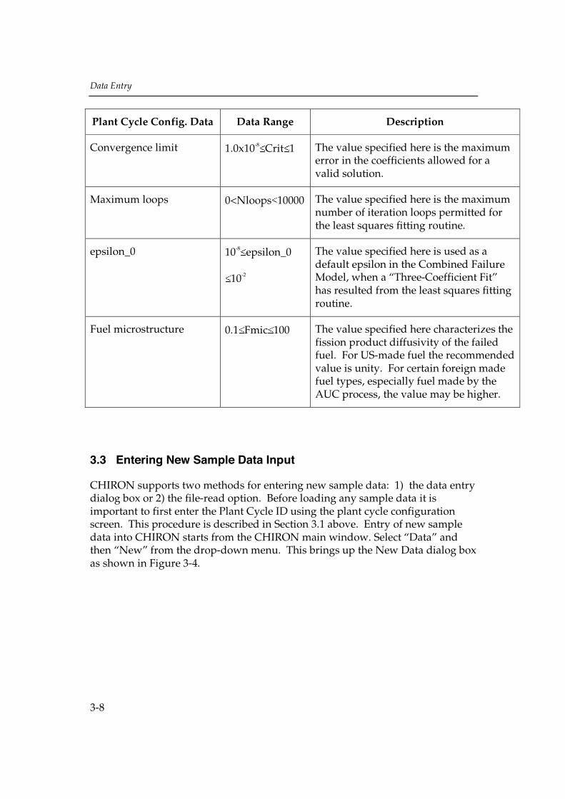
Convergence limit 1.0x10⁻⁸ Crit 1 The value specified here is the maximumerror in the coefficients allowed for avalid solution.
Maximum loops 0<Nloops 10000 The value specified here is the maximumnumber of iteration loops permitted forthe least squares fitting routine.
epsilon_0 10-8 epsilon_0
10-2
The value specified here is used as adefault epsilon in the Combined FailureModel, when a “Three-Coefficient Fit”has resulted from the least squares fittingroutine.
Fuel microstructure 0.1 Fmic 100 The value specified here characterizes thefission product diffusivity of the failedfuel. For US-made fuel the recommendedvalue is unity. For certain foreign madefuel types, especially fuel made by theAUC process, the value may be higher.
3.3 Entering New Sample Data Input
CHIRON supports two methods for entering new sample data: 1) the data entrydialog box or 2) the file-read option. Before loading any sample data it isimportant to first enter the Plant Cycle ID using the plant cycle configurationscreen. This procedure is described in Section 3.1 above. Entry of new sampledata into CHIRON starts from the CHIRON main window. Select “Data” andthen “New” from the drop-down menu. This brings up the New Data dialog boxas shown in Figure 3-4.

Data Entry
3-9
Figure 3-4New Data Dialog Box
The input methods available for entering new sample data are “Screen” and“File”, selectable by the radio-buttons. “Screen” is intended for single sampleinput, “File” for multiple sample (batch) input. The following subsections dealwith each of these input methods separately.
3.3.1 Single Sample Activity Data Input
Before entering sample data, verify the data units that are currently in effect. Todo this, click on “Edit Units”. The Sample Data Units dialog box appears (seeFigure 3-5).

Data Entry
3-10
Figure 3-5Sample Data Units Dialog Box
If the input units shown in the list-boxes of the Sample Data Units dialog box arethe ones desired then the box is closed by clicking “Cancel”. Otherwise, alternateunits may be selected by holding down on the arrow next to each data unit. Inthe case shown in Figure 3-5, the list-box for Reactor Power Units has beenopened. The available choices are shown in the scroll list and include: “FracP”for fractional power (normally between 0 and 1), “%P” for percent power(normally between 0 and 100), and “MWth” for absolute power in MWth. Theasterisks in parentheses indicate that these are cardinal units that CHIRON usesinternally. CHIRON converts from the selected units to the appropriate cardinalunits, using built-in conversion factors.
If changes are made to any of the items in the Sample Data Units dialog box, clickOK to accept the changes. Choose “Cancel” to go back to the New Data screenwithout accepting any changes.
Now you are ready to enter data. To enter Single Sample Input, click “Screen”from the New Data dialog box, then OK. The Add Sample dialog box appears asshown in Figure 3-6.

Data Entry
3-11
Figure 3-6Add Sample Dialog Box
Input units are shown by each value to remind the user of the current settings.Table 3-2 provides definitions for the sample data entry fields entered on thisscreen.

Data Entry
3-12
Table 3-2.Sample Data Input Units
Sample Data Input Data Range Description
Plant Cycle ID xxxxx-nn The Plant Cycle ID must coincide with oneavailable in the database. Its format is a 5-character text-string (Plant Name), followed bya hyphen (“-”), followed by a single or doubledigit number (Cycle Number). The plant nameis case sensitive. Do not use a leading zero in asingle digit cycle number.
Sample Date mm/dd/yy The sample date entered in the formMM/DD/YY.
Sample Time hh:mm:ss The sample time entered in the formHH:MM:SS.
Reactor Power 0 RxPow 10 inFracP
The current reactor power (as opposed to ratedpower).
Clean-up Flow 0< ClFlow 10000in gal/min
The cleanup or letdown flow rate (required forconversion of Ci/ml to Ci/sec).
Rod Power Factor 0<RPF 10 The ratio of the linear heat-rating of the failedfuel, if any, to the average linear heat rating ofthe entire core, at the current reactor power level.For File Read input, occurrences of RPF = 0 willbe replaced by the default value 1.08.
Burnup 0 BU 1000 inMWd/kgU
An estimate of the burnup of the failed fuel.
Gas Delay Time -5000 DelTime50000 in seconds
Any delay that may occur between activityrelease for offgas isotopes at the fuel breach,and sample capture. The delay due to coolantcirculation time is usually negligible.

Data Entry
3-13
Sample Data Input Data Range Description
I Delay Time -5000 DelTime50000 in seconds
Applies to the iodines, and is otherwise definedas above for the offgas isotopes.
Sol Delay Time -5000 DelTime50000 in seconds
Applies to the reactor solubles, and is otherwisedefined as above for the offgas isotopes.
SJAE (Steam Jet AirEjector) Gas Flow
For BWRs:500 SJAEFlow
50000 in cc/sec
For PWRs:SJAEFlow=0
The flow rate of the steam in the bypass linethat drives the evacuation of non-condensablegases from the condenser, by means of a jetnozzle. The flow rate is used for BWRs as aconversion factor between measured activity in
Ci/cc and release rate activity in Ci/sec.
Offgas Activities volumetric units:0 Abs VolOGAct
1.e6 in Ci/cc
release-rate units:0 Abs RrOGAct
5.e8 in Ci/sec
Measured activity of the offgas or noble gasisotopes. A negative value for an isotopicactivity has the effect of omitting the activityvalue from the R/B fit and subsequent fuelfailure evaluations, although the measurementvalue is retained in the CHIRON database forreference purposes.
Iodine Activities volumetric units:0 Abs VolIOAct
1.e6 in Ci/cc
release-rate units:0 Abs RrIOAct
5.e8 in Ci/sec
Measured activity of the iodine isotopes. Anegative value for an isotopic activity has theeffect of omitting the activity value from theR/B fit and subsequent fuel failure evaluations,although the measurement value is retained inthe CHIRON database for reference purposes.
Rx SolublesActivities
volumetric units:0 VolSolAct 1.e6in Ci/cc
release-rate units:0 RrSolAct 5.e8 in Ci/sec
Measured activity of the selected reactorsoluble isotopes. Reactor solubles cannot beincluded in R/B fit and, therefore, are alwaysnon-negative values.
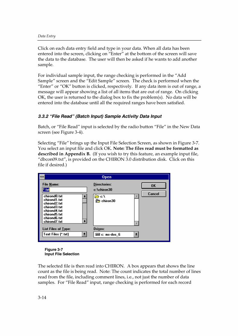
Data Entry
3-14
Click on each data entry field and type in your data. When all data has beenentered into the screen, clicking on “Enter” at the bottom of the screen will savethe data to the database. The user will then be asked if he wants to add anothersample.
For individual sample input, the range checking is performed in the “AddSample” screen and the “Edit Sample” screen. The check is performed when the“Enter” or “OK” button is clicked, respectively. If any data item is out of range, amessage will appear showing a list of all items that are out of range. On clickingOK, the user is returned to the dialog box to fix the problem(s). No data will beentered into the database until all the required ranges have been satisfied.
3.3.2 “File Read” (Batch Input) Sample Activity Data Input
Batch, or “File Read” input is selected by the radio button “File” in the New Datascreen (see Figure 3-4).
Selecting “File” brings up the Input File Selection Screen, as shown in Figure 3-7.You select an input file and click OK. Note: The files read must be formatted asdescribed in Appendix B. (If you wish to try this feature, an example input file,“dbcon09.txt”, is provided on the CHIRON 3.0 distribution disk. Click on thisfile if desired.)
Figure 3-7Input File Selection
The selected file is then read into CHIRON. A box appears that shows the linecount as the file is being read. Note: The count indicates the total number of linesread from the file, including comment lines, i.e., not just the number of datasamples. For “File Read” input, range checking is performed for each record

Data Entry
3-15
read, and any non-compliances are posted to the screen as they occur. In suchcases, the user is advised of the problem and given the choice to either stop theread-in or to continue. None of the non-compliant records are transferred to thedatabase.
If the file is read successfully, a list-box appears to show only the newly enteredsamples. This box is equivalent to the Samples Selection Box of Figure 2-17.Samples analysis may proceed from this box, in the manner previously explainedin Section 2.5, Step 9 .To generate a list box containing all samples for the cycle,close this box and open the plant cycle again (see Section 2.5, Step 5).
Alternatively, batch input files may be created by organizing sample data in aspreadsheet, such as Microsoft Excel, according to the format shown inAppendix B, then saving the spreadsheet as a comma-separated text file usingthe “Save As” option from the spreadsheet file menu.

Data Entry
3-16

4-1
4 CHIRON OUTPUT
This section discusses the various output produced by CHIRON. With CHIRONthe user can generate single-sample screen plots, various trending plots, screenreports and printed reports. Descriptions of the plot and report options aredescribed in the subsections that follow. Illustrations of each type of plot andreport are provided.
Plots and reports can be edited, copied to hard-disk as a bit-map file and/orprinted to any printer installed under WINDOWS. By clicking on the rightmouse button from anywhere inside a graph display, the user can access a menucontaining numerous graphic display options that allow customization of theCHIRON plot. The user can modify the gridlines, font size, color, data labels,and more. Printing is controlled from the Export Dialog option, while editing isnormally performed from the Customization Dialog option. A description ofthese plot options is provided in Section 2 in Table 2-1. By clicking on the “Help”option in the right mouse button menu, you can also access more information onthese plot options.
4.1 Single-Sample Screen Plots
The list of available single-sample screen plots is shown below:
Release to Birth (R/B) vs. Lambda for Offgas and Iodines
R/B vs. Lambda for Solubles
Cesium Ratio vs. Predicted Burnup
F(Epsilon) vs. Epsilon
C vs. Epsilon
Failure Correlation Epsilon vs. A Epsilon
Y versus X plot
These plots are accessed from the drop-down menu of the Analysis Summaryscreen (see Figure 2-19). The following subsections explain each plot in detailand provide illustrations of sample plots.

CHIRON Output
4-2
4.1.1 The R/B versus Plot, Offgas and Iodines
An example of the Release to Birth (R/B) vs. Lambda for offgas and iodines plotis shown in Figure 4-1. It contains a base-line curve (representing tramp) and atotal activity curve (representing tramp plus failed fuel) for offgas, and a similarpair for iodines. The separation between the total and tramp activity, i.e., the riseof the R/B over the base-line, represents the failed fuel activity. Gridlines wereadded to this plot by using the menu option “Gridlines”, available by clickingthe right mouse button.
Figure 4-1R/B versus Plot for Offgas and Iodines
For a typical sample, the offgas curves will tend to be higher than the iodinescurves, due to the fact that iodines have more chemical affinity to other elementsthan do the noble gases. Thus, the behavior of the noble gases represent a closeto ideal diffusion behavior, while the iodine activities may be attenuated becauseof reactions with other materials.
However, the separation between the offgas and iodines curves is temperaturedependent, such that the separation tends to be smaller for higher temperaturefailed fuel.
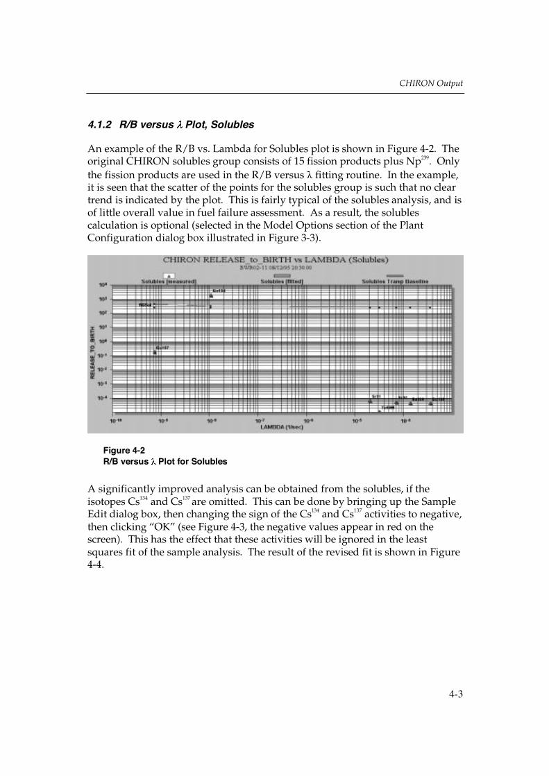
CHIRON Output
4-3
4.1.2 R/B versus Plot, Solubles
An example of the R/B vs. Lambda for Solubles plot is shown in Figure 4-2. Theoriginal CHIRON solubles group consists of 15 fission products plus Np239. Onlythe fission products are used in the R/B versus fitting routine. In the example,it is seen that the scatter of the points for the solubles group is such that no cleartrend is indicated by the plot. This is fairly typical of the solubles analysis, and isof little overall value in fuel failure assessment. As a result, the solublescalculation is optional (selected in the Model Options section of the PlantConfiguration dialog box illustrated in Figure 3-3).
Figure 4-2R/B versus Plot for Solubles
A significantly improved analysis can be obtained from the solubles, if theisotopes Cs134 and Cs137 are omitted. This can be done by bringing up the SampleEdit dialog box, then changing the sign of the Cs134 and Cs137 activities to negative,then clicking “OK” (see Figure 4-3, the negative values appear in red on thescreen). This has the effect that these activities will be ignored in the leastsquares fit of the sample analysis. The result of the revised fit is shown in Figure4-4.

CHIRON Output
4-4
Figure 4-3Sample Edit Screen Showing Deletion of Two Cs-Activities
Figure 4-4Revised R/B versus Plot for Solubles
It is envisaged that specific scenarios exist in which solubles analyses will provevery valuable, in particular when applied to certain subsets of solubles. Further

CHIRON Output
4-5
development is anticipated in this area. For the present, however, it isrecommended that the solubles analysis be switched off for routine analyses.This is the default choice in the Add Plant Configuration dialog box, see Figure3-3).
4.1.3 Cs-Ratio versus Predicted Burnup
The ratio of the two cesium activities Cs134 and Cs137 can be used to estimate theburnup of the failed fuel. When the Cs-ratio burnup plot is chosen, the dialogbox shown in Figure 4-5 appears.
Figure 4-5Selection of Burnup Model for Cs-Ratio Burnup Prediction
The user may now select a “Plant Cycle History”. The Plant Cycle History refersto a set of reference ORIGEN curves that are dependent on the plant type, cyclelength, outage schedule, enrichment, and reactor power. These curves areavailable to compare the Cs ratio calculated by CHIRON to some reference cases.The user can select an option, click OK, and a plot similar to Figure 4-6 will bedisplayed. The CHIRON model is shown as the smooth curve, while the othercurve represents the ORIGEN curve.

CHIRON Output
4-6
Figure 4-6Cs-Ratio versus Predicted Burnup
4.1.4 f( ) versus Plot
The f( ) versus relationship is the fundamental expression in the CHIRONleast-squares fitting routine (for the theoretical derivation, see Chapter 6).CHIRON seeks the root of this curve, which is then accepted as the calculated .f( ) may have more than one root, as seen in Figure 47. If this is the case, thelower of the two values is the physically meaningful one.
The f( ) versus relationship plot is included in CHIRON to allow the user toscrutinize sample analyses for their detailed numerical behavior. The plotincludes three curves depicting the offgas, iodines and solubles analyses. Theroots determined by CHIRON are marked on the plot for each isotopic group.
To study details of the plot, use the zoom feature. Zooming is accomplished bydepressing the left mouse button at the upper left corner of the rectangle thatdefines the desired view, then dragging to the lower right corner and releasing.To get out of the zoomed view, select the menu item “Undo Zoom”, available byclicking the right mouse button anywhere in the graph area.

CHIRON Output
4-7
Figure 4-7f( ) versus Plot
4.1.5 C( ) versus Plot
The C( ) plot (Figure 4-8) is shown to support the understanding of the wayCHIRON accepts or rejects a fit analysis. Normally, CHIRON calculates threecoefficients: “ ”, “A ” and “C”. Sometimes, however, the analysis defaults toproviding only two coefficients. This happens for instance when the “C”coefficient turns out negative for the calculated . This would correspond tonegative tramp (see Chapter 6), and is, therefore, not acceptable. Thus, CHIRONwill discard the “three-coefficient fit” and instead present a “two-coefficient fit”,based on recalculated values of C and A (see Chapter 6 for details).
The C( ) plot enables the user to see how the coefficient C varies with epsilon.For an acceptable “three-coefficient fit”, the C-value at the calculated epsilon,must be positive. The calculated epsilons are marked in the C-plot for eachisotopic group. The plot will attempt to show C-coefficient curves for all threeisotopic groups, if calculated. However, in some cases scaling may result in thedisappearance of some curves from view. The zoom feature described earlier inthis section can then be used to study the detail on the plot.

CHIRON Output
4-8
Figure 4-8C( ) versus Plot
4.1.6 Failure Correlation Plot
The correlation provided in CHIRON to estimate the number of failed fuel rodsutilizes an empirical fit that relates the a and coefficients to the number of fuelfailures. The third coefficient, “C”, is used to correct the nuclide activity forrecoil release, and is not directly used in the failure correlations.
The failure correlation plot displays the current sample coefficients relative to theboundaries of available model data used to develop the failure correlation for theappropriate reactor type. Failure correlation for sample data points that liewithin the corresponding boundary are generally perceived to be more reliable.
Figure 4-9 shows a typical failure correlation plot for a BWR data sample.

CHIRON Output
4-9
Figure 4-9Failure Correlation Plot for BWRs
4.1.7 User Defined X Versus Y Plot
The last sample plot to discuss is the User Defined X versus Y plot. This is ageneral plot. It is intended to be user defined, with the user selecting from listsof allowable options. This choice is not currently available and, therefore,appears grayed out in the drop-down menu.
4.1.8 Editing Single-Sample Screen Plots
Single-sample screen plots are edited, exported, or printed in the same way asdescribed in Section 2.5 , Steps 11 and 12 for the trending plots.
4.2 Trending Plots
Trend plots are available immediately after performing a batch analysis or byselecting the Trend Plots option from the trending menu. Selecting the optionfrom the trending menu will generate a plot based on the cases already analyzedin the database.

CHIRON Output
4-10
4.2.1 Standard Trending Plots
Trend plots are selected from the dialog box shown in Figure 2-22. Each of thetwo list-boxes (one for the Y Axis and one for the X axis) contains 86 selectablefunctions for plotting. These are described below.
Selection # Selection Title Description
0 Power Fraction of Rated Reactor Power1 Xe-138 (rel rate) Non-Fitted Activity, Ci/sec2 Xe-135m (rel rate) Non-Fitted Activity, Ci/sec3 Kr-87 (rel rate) Non-Fitted Activity, Ci/sec4 Kr-88 (rel rate) Non-Fitted Activity, Ci/sec5 Kr-85m (rel rate) Non-Fitted Activity, Ci/sec6 Xe-135 (rel rate) Non-Fitted Activity, Ci/sec7 Xe-133 (rel rate) Non-Fitted Activity, Ci/sec8 I-134 (rel rate) Non-Fitted Activity, Ci/sec9 I-132 (rel rate) Non-Fitted Activity, Ci/sec10 I-135 (rel rate) Non-Fitted Activity, Ci/sec11 I-133 (rel rate) Non-Fitted Activity, Ci/sec12 I-131 (rel rate) Non-Fitted Activity, Ci/sec13 Tc-101 (rel rate) Non-Fitted Activity, Ci/sec14 Ba-141 (rel rate) Non-Fitted Activity, Ci/sec15 Cs-138 (rel rate) Non-Fitted Activity, Ci/sec16 Ba-139 (rel rate) Non-Fitted Activity, Ci/sec17 Sr-92 (rel rate) Non-Fitted Activity, Ci/sec18 Tc-99m (rel rate) Non-Fitted Activity, Ci/sec19 Sr-91 (rel rate) Non-Fitted Activity, Ci/sec20 Np-239 (rel rate) Non-Fitted Activity, Ci/sec21 Mo-99 (rel rate) Non-Fitted Activity, Ci/sec22 Te-132 (rel rate) Non-Fitted Activity, Ci/sec23 Ba-140 (rel rate) Non-Fitted Activity, Ci/sec24 Te-129m (rel rate) Non-Fitted Activity, Ci/sec25 Sr-89 (rel rate) Non-Fitted Activity, Ci/sec26 Cs-134 (rel rate) Non-Fitted Activity, Ci/sec27 Sr-90 (rel rate) Non-Fitted Activity, Ci/sec28 Cs-137 (rel rate) Non-Fitted Activity, Ci/sec29 Xe-138/I-131 Non-Fitted Activity (rel rate) Ratio30 I-131/Xe-133 Non-Fitted Activity (rel rate) Ratio31 I-134/I-131 Non-Fitted Activity (rel rate) Ratio

CHIRON Output
4-11
Selection # Selection Title Description
32 Xe-138/Xe-133 Non-Fitted Activity (rel rate) Ratio33 Cs-134/Cs-137 Non-Fitted Activity (rel rate) Ratio34 Sr-90/Sr-92 Non-Fitted Activity (rel rate) Ratio35 Np-239/(Sum15+Np) Non-Fitted Activity (rel rate) Ratio36 OG Sum-of-Six Non-Fitted Release Rates, Ci/sec37 OG Sum-of-Six Fitted Release Rates, Ci/sec38 OG Sum6 Tramp Fitted Release Rates, Ci/sec39 OG Sum6 nonTramp Fitted Release Rates, Ci/sec40 ID Sum-of-Five Non-Fitted Release Rates, Ci/sec41 ID Sum-of-Five Fitted Release Rates, Ci/sec42 ID Sum5 Tramp Fitted Release Rates, Ci/sec43 ID Sum5 nonTramp Fitted Release Rates, Ci/sec44 Solubles Sum Non-Fitted Release Rates, Ci/sec45 Solubles Sum Fitted Release Rates, Ci/sec46 Solubles Tramp Fitted Release Rates, Ci/sec47 Xe-138 (rel rate) Fitted Release Rate Activity, Ci/sec48 Xe-135m (rel rate) Fitted Release Rate Activity, Ci/sec49 Kr-87 (rel rate) Fitted Release Rate Activity, Ci/sec50 Kr-88 (rel rate) Fitted Release Rate Activity, Ci/sec51 Kr-85m (rel rate) Fitted Release Rate Activity, Ci/sec52 Xe-135 (rel rate) Fitted Release Rate Activity, Ci/sec53 Xe-133 (rel rate) Fitted Release Rate Activity, Ci/sec54 I-134 (rel rate) Fitted Release Rate Activity, Ci/sec55 I-132 (rel rate) Fitted Release Rate Activity, Ci/sec56 I-135 (rel rate) Fitted Release Rate Activity, Ci/sec57 I-133 (rel rate) Fitted Release Rate Activity, Ci/sec58 I-131 (rel rate) Fitted Release Rate Activity, Ci/sec59a Epsilon OG Calculated by Least Sqs. Fit to OG59b Epsilon ID Calculated by Least Sqs. Fit to ID60a AEpsilon OG Calculated by Least Sqs. Fit to OG60b AEpsilon ID Calculated by Least Sqs. Fit to ID61a C OG Calculated by Least Sqs. Fit to OG61b C ID Calculated by Least Sqs. Fit to ID62a Fit Error OG R-squared Goodness of Fit, OG62b Fit Error ID R-squared Goodness of Fit, ID63a PuFrac OG Pu-239 Fission Yield Ratio from OG63b PuFrac ID Pu-239 Fission Yield Ratio from ID64a Failures OG No. of Failures by Gen. OG Model64b Failures ID No. of Failures by Gen. ID Model65 Comb. Model Fail. Number of Failed Rods by CFM

CHIRON Output
4-12
Selection # Selection Title Description
66 Comb. Model RPF Rod Pwr Fact. Calculated by CFM67 Sample RPF Inputted Sample Rod Power Factor68 INPO FRI “Daily FRI”, Regardless of Power69 N-13 (rel rate) Non-Fitted Activity, Ci/sec70 Rb-89 (rel rate) Non-Fitted Activity, Ci/sec71 Nb-97 (rel rate) Non-Fitted Activity, Ci/sec72 Ar-41 (rel rate) Non-Fitted Activity, Ci/sec73 Cu-64 (rel rate) Non-Fitted Activity, Ci/sec74 Na-24 (rel rate) Non-Fitted Activity, Ci/sec75 Zr-97 (rel rate) Non-Fitted Activity, Ci/sec76 Y-90 (rel rate) Non-Fitted Activity, Ci/sec77 Cr-51 (rel rate) Non-Fitted Activity, Ci/sec78 Fe-59 (rel rate) Non-Fitted Activity, Ci/sec79 Hf-181 (rel rate) Non-Fitted Activity, Ci/sec80 Zr-95 (rel rate) Non-Fitted Activity, Ci/sec81 Co-58 (rel rate) Non-Fitted Activity, Ci/sec82 Zn-65 (rel rate) Non-Fitted Activity, Ci/sec83 Mn-54 (rel rate) Non-Fitted Activity, Ci/sec84 Co-60 (rel rate) Non-Fitted Activity, Ci/sec85 Sample BU Burnup Calculated from Sample
Note, that Selections 59-64 are all double selections. This means that the itemsnamed as “a” and “b” are selected together and co-plotted in the same graph.
4.2.2 User Defined Trending Plots
User-defined trending plots are intended to enable the user to plot a wideselection of activities, or expressions based on activities, as functions of time or asfunctions of other such expressions. This option is not currently available.
4.2.3 Editing Trending Plots
Editing, exporting, and printing of trend-plots is described in Section 2.5, Steps11 and 12.
4.3 Screen Reports
The list of available single-sample screen reports is shown below:

CHIRON Output
4-13
Offgas Activity and Fit Summary
Iodine Activity and Fit Summary
Solubles Activity and Fit Summary
Offgas RB Summary
Iodines RB Summary
Solubles RB Summary
Activity Ratio Summary
QA Report
These reports are accessed from the drop-down menu of the Analysis Summaryscreen (see Figure 2-20). In addition, a general CHIRON information screenreport is available from the CHIRON main window by clicking on “Help” andthe “About CHIRON” option.
The following subsections explain each report in detail and provide illustrationsof sample reports.
4.3.1 Offgas Activity Summary Report
The Offgas Activity Summary screen report shows both the measured activitiesand the corresponding values on the best fit curve for the analyzed sample. Thescreen also shows the values of all three fit coefficients, the R2-value (statistical“Goodness of Fit” parameter, see Chapter 6), the final convergence error, and thenumber of iterations needed for convergence. A sample Offgas ActivitySummary screen report is shown in Figure 4-10.
Notably, this screen does not report the Pu239 yield fraction that results from thesample analysis, nor does it report whether the “three-coefficient fit” wasaccepted or not. This information is found in the Sample Analysis and FitSummary screen.
Reasons for fit rejection are non-convergence, or a negative C-value, resultingfrom the least-squares analysis. In any of these events the -value will be set tozero, and a two-coefficient fit will then be provided. The “C” and “A ”coefficients from that calculation will then be the values reported in the presentscreen. If the C-value is still negative, the sample will be rejected. In batchanalysis, such samples will be left out of the trending analysis.

CHIRON Output
4-14
Figure 4-10Offgas Activity Summary Report
4.3.2 Iodines Activity Summary Report
The Iodines Activity Summary screen report is analogous to the Offgas ActivitySummary screen report discussed in the previous subsection. A sample IodinesActivity Summary screen report is shown in Figure 4-11.
Figure 4-11Iodines Activity Summary Report

CHIRON Output
4-15
4.3.3 Solubles Activity Summary Report
The Solubles Activity Summary screen report is analogous to the Offgas ActivitySummary screen report. See Section 4.3.1 for a discussion. It is noted that thisreport only displays eight out of the 15 fission product solubles activities. Asample Solubles Activity Summary screen report is shown in Figure 4-12.
Figure 4-12Solubles Activity Summary Report
4.3.4 Offgas Release to Birth Summary Report
The Offgas Release to Birth Summary screen report shown in Figure 4-13presents the offgas datapoints, both measured and fitted, that appear in theOffgas and Iodines R/B versus plot (Figure 4-1 in Section 4.1.1).
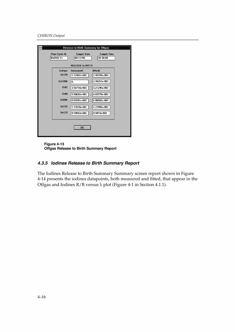
CHIRON Output
4-16
Figure 4-13Offgas Release to Birth Summary Report
4.3.5 Iodines Release to Birth Summary Report
The Iodines Release to Birth Summary Summary screen report shown in Figure4-14 presents the iodines datapoints, both measured and fitted, that appear in theOffgas and Iodines R/B versus plot (Figure 4-1 in Section 4.1.1).

CHIRON Output
4-17
Figure 4-14Iodines Release to Birth Summary Report
4.3.6 Solubles Release to Birth Summary Report
The Solubles Release to Birth Summary screen reportshown in Figure 4-15presents a selection of eight out of the 15 fission product solubles activities, bothmeasured and fitted, that appear in the Solubles R/B versus plots (Figure 4-2and 4-4 in Section 4.1.2).

CHIRON Output
4-18
Figure 4-15Solubles R/B versus Fit Summary Report
4.3.7 The Activity Ratio Summary Report
The Activity Ratio Summary Report (Figure 4-16) shows important activity ratiosfor the sample, as well as the burnup value calculated from the Cs-ratio, whenavailable.
Figure 4-16Activity Ratio Summary Report

CHIRON Output
4-19
4.3.8 The QA Report
The QA report provides all input and output data for the current single-sampleanalysis, including plant configuration data, model parameter selections,calculational options settings, model versions, and model constants. This file isintended to provide a complete QA record for any single sample, so that thecalculation may be reproduced independently of the current database. Thisreport is created upon request by selecting “Generate QA Report” or “Generateand View QA Report” from the “Reports” drop-down menu of the Analysis FitSummary Results screen (see Figure 2-20).
4.3.9 The CHIRON Configuration Screen Report
The CHIRON Configuration report provides the revision history for theCHIRON code. This report is accessed from the CHIRON main window byclicking on “Help” and selecting the “ About CHIRON” menu option.
4.4 Printed Reports
4.4.1 The QA Report
The QA report described in Section 4.3.8 can be printed. An example of acomplete report text is shown in Appendix C.
4.4.2 The Calculation Log Report
The Calculation Log Report is available for single sample analysis only. Togenerate the log report, the “Enable calculation log file” box must be checked inthe Output Options screen. (Accessed in main window under “options” menu,“Output Options” option.) A log report is generated for every single sampleanalysis performed until you disable (uncheck) the box in the Output Optionsscreen. The log report file is overwritten for each new sample analyzed.
The Calculation Log Report is written to a text-file named “chicalc.log” whichcan be read into and printed by any text editor. The “chicalc.log” file can belarge, on the order of 60 printed pages. This file is primarily of use fordebugging purposes.
4.4.3 The ASCII Dump Files
The ASCII Dump Files can be generated for batch sample analysis only. A totalof ten ASCII files are generated when this option is invoked. A detailed

CHIRON Output
4-20
description of the generation, use, format, and contents of these 10 ASCII dumpfiles is provided in Appendix D.

5-1
5 THE CHIRON DATABASE
5.1 Database Overview
CHIRON is designed around a relational database system for the storage of theraw data and the analysis results. This allows the user to easily access andanalyze the individual samples and to observe trends in the data through thetrend plot features.
In order to provide flexibility in the database platform, CHIRON accesses datathrough a standard interface with ODBC 2.1 drivers. The ODBC interface allowsCHIRON to access a variety of different database formats through a commoninterface. With this interface, CHIRON users can maintain their data in aMicrosoft Access, Oracle, Paradox, or other database format that has an ODBCdriver. CHIRON was developed using the Microsoft Access driver and all of thesample databases are in this format. The ODBC 2.1 driver for Microsoft Accesscorresponds to Microsoft Access Version 2.0. CHIRON has not been tested withany other database platform.
5.2 Database Structure
The CHIRON database is made up of six tables: samples, plant_data, failures,user_preferences, units, and unit_types. The contents of each of the tables issummarized below, but the detailed list of all of the data fields can be found inAppendix E.
The samples table contains all of the coolant sample data. This includes thesample date, reactor power, and the activity level for each of the nuclides. Thistable also contains the units defined for each value at the time the sample wasentered. The data in this table corresponds with the data shown on the AddSample dialog box (see Figure 3-6).
The plant_data table contains the plant specific data that does not change duringa plant cycle. This includes the plant type (BWR or PWR), rated power, numberof fuel rods, etc. as well as flags and other values that impact the calculation.
The CHIRON Database
5-2
The failures table contains the results of the analysis for each of the samples. Thevalues include the fit coefficients determined by the calculation and the activitylevels for each of the nuclides.
The user_preferences table contains the units that the user has requested forfuture data input. This may be changed at any time by the user, but changingthe units does not affect samples previously entered into the database.
The units table contains a list of the available units and the conversion factors toconvert the input value to the cardinal unit. CHIRON reads this table to obtainthe conversion factors.
The unit_types table provides a map of which units are available for each unitcategory. For example, the reactor power can be entered in either %P, FracP, orMWth. This table, in conjunction with the units table, generates the pull downboxes on the Sample Data Units dialog box (see Figure 3-5).
5.3 Creating a New Database
The typical CHIRON installation installs a blank database, chiblank.mdb,containing no data so that users can generate their own databases. It is highlyrecommended that users make a copy of the blank database before adding datato it. The following steps create a new database called PlantA:
1. Using File Manager (File|Copy) or the copy command from an MS-DOSprompt, copy “chiblank.mdb” to “planta.mdb”.
2. Start the CHIRON program and select Select Data Source from the Datamenu.
3. From the SQL Data Sources Dialog, select New. From this point on, the stepsare shown in detail in Section 2, steps 7.B through 7.D using PlantA as thedata source name and planta.mdb as the database name. The steps arequickly summarized below in steps 4-7.
4. Select the Microsoft Access Driver and click OK.
5. Register the database as PlantA and click Select.
6. Select planta.mdb and click OK.
7. Check that you are registering planta.mdb as PlantA and click OK.
8. Select PlantA and click OK. The new database is now open.
9. From the CHIRON main window, add a plant configuration record bychoosing the Options menu|Plant Configuration|Add New Plant.
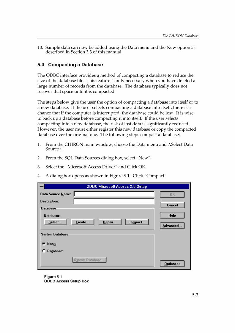
The CHIRON Database
5-3
10. Sample data can now be added using the Data menu and the New option asdescribed in Section 3.3 of this manual.
5.4 Compacting a Database
The ODBC interface provides a method of compacting a database to reduce thesize of the database file. This feature is only necessary when you have deleted alarge number of records from the database. The database typically does notrecover that space until it is compacted.
The steps below give the user the option of compacting a database into itself or toa new database. If the user selects compacting a database into itself, there is achance that if the computer is interrupted, the database could be lost. It is wiseto back up a database before compacting it into itself. If the user selectscompacting into a new database, the risk of lost data is significantly reduced.However, the user must either register this new database or copy the compacteddatabase over the original one. The following steps compact a database:
1. From the CHIRON main window, choose the Data menu and Select DataSource .
2. From the SQL Data Sources dialog box, select “New”.
3. Select the “Microsoft Access Driver” and Click OK.
4. A dialog box opens as shown in Figure 5-1. Click “Compact”.
Figure 5-1ODBC Access Setup Box

The CHIRON Database
5-4
5. A new box appears similar to that shown in Figure 5-2. Select a database youwould like to compact from the list of database names and click OK.
Figure 5-2Compact Database Dialog Box
6. To compact the database into itself, select the same database name from thedialog box and click OK. Alternatively, the user can type in a new databasename and click OK. If a new name is selected, that name must be registeredbefore it can be used by CHIRON.
7. If you chose to compact the database into itself, a warning box will appearinforming you that you are about to overwrite an existing file. Click Yes ifthis is what you want to do.
8. The compacting process begins and when it is finished a box appears tellingyou it compacted the database successfully.
5.5 Converting a CHIRON 2.3 Database to CHIRON 3.0
The database conversion program DBConv reads in a set of six ASCII files (the"ASCII Dump") created by CHIRON for DOS, Version 2.2 or later and writes outa single file containing all of the raw sample input data. The ASCII files must beavailable in the directory containing CHIRON for WINDOWS. The ASCII Dumpfilenames consist of a character string (up to 7-characters provided by the user)followed by a number from zero to five, and with the file extension ".csv".
To use DBConvert, double click on the DBConvert icon from the CHIRON groupin the WINDOWS program manager. A MS-DOS window appears. DBConvertprompts the user for the following information:

The CHIRON Database
5-5
1. The base name of the CHIRON output (ASCII dump) files. This is the 7-character string entered above. After entering the characters, press “Enter”and you will be prompted for the next item.
2. The Plant Identifier as it appears in CHIRON (up to five-character string).Note this is case sensitive.
3. The Cycle Identifier as an integer.
4. The SJAE Flow, in cc/sec. This number is only needed for BWRs. If theplant is a PWR, enter zero.
DBConvert generates an output file with one line for each sample date/time,which will represent a record in the database. The output filename is formed bycombining the plant name string, the plant cycle number, and an extension .txt(e.g. Susq09.txt) Each record in the file is assigned the user supplied plant nameand cycle number. DBConvert expects the data in the ASCII dump files to befrom one plant cycle.
* * * Note: The user specified plant name is used to generate the "Plant-cycle ID"for the ACCESS database. Since the Plant-cycle ID is used in ACCESS in a case-sensitive manner, it is important that the user specified five-character PlantIdentifier be entered exactly (case sensitive) as it is to appear in the PlantConfiguration table within ACCESS.
The output file generated by DBConvert is a valid "File Read" input file toCHIRON for WINDOWS. Before reading the file into CHIRON for Windows,the user must create a "Plant Configuration" entry for the plant-cycle beingloaded. This is provided through the Add Plant Configuration dialog box inCHIRON. The configuration information can best be retrieved from the "QA"report, printable from the CHIRON DOS version after completing any singlesample analysis within the Plant-cycle ID data set. The "QA" report is found inthe CHIRON DOS version under the menu "Reports", submenu "Hard CopyReports".
Follow the instructions in Section 3 for the File Read input option to CHIRON.

The CHIRON Database
5-6

6-1
6 CHIRON THEORY
The theoretical basis for the CHIRON analysis is contained in References 1-3.This section presents all the logical steps in the mathematical derivations,including a discussion of the limiting assumptions made.
6.1 FORMULATION OF THE BASIC EQUILIBRIUM EQUATIONS
The change in inventory with time of a given radioactive nuclide, subscripted i,in the reactor coolant in the presence of X failed fuel rods can be written in termsof the primary production and removal components as:
dNdt
N N Nic
k
X
ikv
ik Ti i ic
1(Eq. 6-1)
where
Nic = number of atoms of nuclide i in the coolant.
Nikv = number of atoms of nuclide i in the void volume of failed rod k.
ik = fraction of atoms of nuclide i released from the void space of failedrod k to the coolant per unit of time.
I = decay constant for nuclide i (1/sec) (see built-in data in Table 6-1).
= primary coolant cleanup rate (1/sec).
= coolant (or steam) carryover rate (1/sec) [= 0 for PWRs].
NTI = rate of isotope deposition to the coolant from tramp sources.

CHIRON Theory
6-2
Table 6-1Isotopic Decay Data and Fission Yields
Isotope Decay Constant, sec-1 Half-life Yield from U235 Yield from Pu239
Xe-138 8.136e-4 14 min. 0.0628 0.0489Xe-135m 7.771e-4 15 min. 0.0106 0.0156
Kr-87 1.520e-4 1.3 hrs. 0.0254 0.0095Kr-88 6.876e-5 2.8 hrs. 0.0358 0.0132
Kr-85m 4.298e-5 4.5 hrs. 0.0131 0.0055Xe-135 2.100e-5 9.2 hrs. 0.0663 0.0747Xe-133 1.517e-6 5.3 days 0.0677 0.0697I-134 2.196e-4 53 min. 0.0761 0.0729I-132 8.426e-5 2.3 hrs. 0.0421 0.0527I-135 2.924e-5 6.6 hrs. 0.0631 0.0641I-133 9.257e-6 21 hrs. 0.0677 0.0693I-131 9.977e-7 8.0 days 0.0284 0.0374
Te-101 8.136e-4 14 min. 0.0504 0.0592Ba-141 6.313e-4 18 min. 0.0587 0.0533Cs-138 3.588e-4 32 min. 0.0672 0.0545Ba-139 1.387e-4 1.4 hrs. 0.0648 0.0564Sr-92 7.105e-5 2.7 hrs. 0.0595 0.0299
Tc-99m 3.198e-5 6.0 hrs. 0.0540 0.0541Sr-91 2.031e-5 9.5 hrs. 0.0592 0.0249
Np-239 3.414e-6 2.3 days 0.0290 0.0290Mo-99 2.916e-6 2.8 days 0.0613 0.0615Te-132 2.468e-6 3.3 days 0.0419 0.0515Ba-140 6.273e-7 13 days 0.0632 0.0557
Te-129m 2.402e-7 33 days 0.0012 0.0027Sr-89 1.589e-7 51 days 0.0485 0.0171
Cs-134 1.067e-8 2.1 yrs. 0.00000045 0.0000032Sr-90 7.579e-10 29 yrs. 0.0592 0.0212
Cs-137 7.302e-10 30 yrs. 0.0626 0.0669N-13 1.16 e-3 10 min. N/A N/ARb-89 7.70 e-4 15 min. not used not usedNb-97 1.60 e-4 1.2 hrs. not used not usedAr-41 1.05e-4 1.8 hrs. N/A N/ACu-64 1.49e-5 13 hrs. N/A N/ANa-24 1.28e-5 15 hrs. N/A N/AZr-97 1.13e-5 17 hrs. not used not usedY-90 3.00e-6 2.7 days not used not usedCr-51 2.88e-7 28 days N/A N/AFe-59 1.78e-7 45 days N/A N/A
Hf-181 1.78e-7 45 days N/A N/AZr-95 1.23e-7 65 days N/A N/ACo-58 1.12e-7 72 days N/A N/AZn-65 3.27e-8 245 days N/A N/AMn-54 2.65e-8 302 days N/A N/ACo-60 4.18e-9 5.3 yrs. N/A N/A
N/A indicates that the isotope is not considered a significant fission product for the CHIRON analysis

CHIRON Theory
6-3
The first term on the right-hand side of Eq. 6-1 represents the isotopecontribution from failed fuel rods. The second term represents the contributionfrom tramp fissions. The third term is the isotopic removal due to decay,cleanup, and, in the case of iodine isotopes in BWRs, carryover with steam.
The number of nuclide atoms in the void volume of a given failed fuel rod can bedetermined from a mass balance of nuclide i within the void region of the failedrod:
dNdt
N Nikv
ikf
ik ik i ikv (Eq. 6-2)
where:
Nikf = number of atoms of nuclide i within the fuel region of rod k at any
instant.
ik = Fraction of atoms of nuclide i released from the fuel into the voidregion of fuel rod k per unit of time.
An expression for the number of atoms of the nuclide in the fuel region of therod, Nik
f , can be developed by considering a mass balance within the fuel region:
dNdt
F y Nikf
k ik ik i ikf (Eq. 6-3)
where:
Fk = fission rate in rod k.
yik = fractional yield of nuclide i per fission in rod k (see data inTable 6-1).
If the analysis is restricted to equilibrium conditions, then the temporalderivative in each of Eqs. 6-1, 6-2 and 6-3 is zero. From the equilibrium form ofEq. 6-3:
N F yikf k ik
ik i(Eq. 6-4)

CHIRON Theory
6-4
If it is assumed that the diffusion rate through the fuel for all isotopes to beconsidered (iodines and noble gases) is much smaller than the nuclide decay rate,then Eq. 6-4 reduces to:
NF y
ikf k ik
i(Eq. 6-5)
The equilibrium form of Eq. 6-2 with Eq. 6-5 substituted for Nikf yields:
N F yikv ik k ik
i ik i(Eq. 6-6)
An expression for the rate of isotope deposition into the coolant from the trampfuel sources ( NTi in Eq. 6-1) can be developed by assuming that the release iscomposed of two components. These components are: (1) direct release of theisotope into the coolant, and (2) diffusional release of the isotopes into thecoolant. The total release rate term can be written as:
tiiTiTiTiT NyFN (Eq. 6-7)
where:
= Fraction of total isotopic production that is released directly to thecoolant.
Ti = Rate of diffusion of the isotope to the coolant.
FTi = Fission rate of the tramp fuel in the core.
yTi = Fractional yield of nuclide i per fission of tramp fuel.
Nti = Isotope concentration resulting from tramp fuel fissions.
The isotope concentration can be determined from a mass balance in the trampdiffusion region:
TiiTiTiTiTi NyF
dtdN 1 (Eq. 6-8)

CHIRON Theory
6-5
The diffusion rate constant Ti should be substantially less than the decay rate(as was the case for diffusion through the fuel pellet). In addition, if steady stateconditions are applied to Eq. 6-8, then the isotopic concentration in the trampdiffusion region becomes:
NF y
TiTi Ti
i
1(Eq. 6-9)
Substitution of Eq. (6-9) into Eq. (6-7) yields:
N F yTiTi
iTi Ti1 (Eq. 6-10)
Substituting Eq. 6-6 and Eq. 6-10 into Eq. 6-1 and considering only theequilibrium form of the equation yields:
i ic
k
Xik ik k ik
i ik i
Ti
iTi TiN F Y F y
11
(Eq. 6-11)
With some approximations and simplifications, Eq. 6-11 can be expressed in aform that will relate the measurement of coolant activity to fuel performance andfailure estimates. Below is a description of the various assumptions applicable toiodine and noble gas coolant activity analysis in light water reactors.
The number of nuclide atoms in the coolant, Nic , in Eq. 6-11, can be determined
from the measured coolant activity concentration, Mic , since
M V Nic
c ic
i (Eq. 6-12)
where:
Mic = measured coolant activity concentration (disintegration/sec/cc).
Vc = volume of water (hot) in the primary coolant system (cc).

CHIRON Theory
6-6
The rod escape rate coefficient, ik, is primarily affected by the size of the defectand the potential for chemical interaction with other elements in the fuel voidregion. For the case of iodine sampling, each nuclide is an isotope of the sameelement (iodine). Thus the chemical interaction for all nuclides can beconsidered to be the same. Similarly, each nuclide in a noble gas sample ischemically inert. Thus the rod escape rate coefficient for a given sample (eitheriodine or noble gas) is independent of the nuclide, i, in that sample. If it isfurther assumed that the defect size does not vary significantly from rod to rod,then the escape rate coefficient is effectively a constant value for all nuclides in aparticular sample (iodine or noble gas) at any given time. Thus, for either aniodine or noble gas sample,
ik = = a constant (Eq. 6-13)
for that particular sample.
If it is further assumed that release from the fuel matrix is diffusion dependent,then the Booth formulation (Reference 4) for diffusional release from the fuelmay be used. Based upon this formulation, the fuel escape rate coefficient isproportional to the square root of the nuclide decay constant:
ik k iD'
where:
D k' = diffusion rate constant for fission products of interest in rod k.
This relationship can be rewritten in the form
ik k ia' (Eq. 6-14)
where:
a k' = a constant including diffusion effects and rod geometry factors.
It should be noted that the geometry factors composing a k' are approximatelyconstant for all light water fuel rods. However, the diffusion effects are affectedby rod temperature and thus a k' does vary somewhat from rod to rod due to thetemperature dependence.

CHIRON Theory
6-7
Similarly, for tramp diffusion,
Ti T iD (Eq. 6-15)
where DT is a Booth diffusion related constant for tramp diffusion. Typical
values for DT are 5.0e-5 sec-1/2 for offgas and 3.5e-5 sec-1/2 for iodines(Reference 5).
The defective rod fission rate factor in rod k, Fk, can be expressed as:
Fk = F fFk (Eq. 6-16)
where:
F = rod fission rate at core average power of an average power fuel rod.
fFk = ratio of fission rate in defective rod k to fission rate of an averagepower rod.
Note that fFk is primarily affected by the ratio of power in rod k to core averagepower, although there may be some secondary effects due to enrichment andburnup difference.
As a final approximation, the nuclide yield term, yik, in Eq. 6-11 can be assumedto be of the form
yik = yi fyk (Eq. 6-17)
where:
yi = fractional yield of nuclide i at an exposure equivalent to the averageexposure of the defective rods in the core.
Fyk = ratio of the nuclide yield for any nuclide in defective rod k to thenuclide yield at the average defective rod exposure.
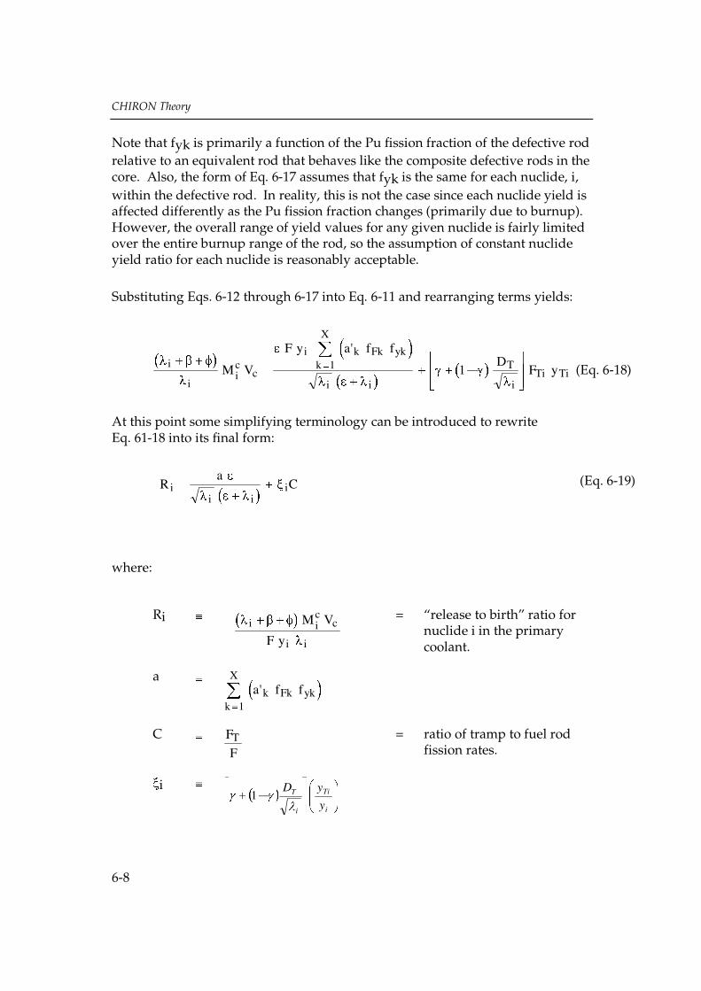
CHIRON Theory
6-8
Note that fyk is primarily a function of the Pu fission fraction of the defective rodrelative to an equivalent rod that behaves like the composite defective rods in thecore. Also, the form of Eq. 6-17 assumes that fyk is the same for each nuclide, i,within the defective rod. In reality, this is not the case since each nuclide yield isaffected differently as the Pu fission fraction changes (primarily due to burnup).However, the overall range of yield values for any given nuclide is fairly limitedover the entire burnup range of the rod, so the assumption of constant nuclideyield ratio for each nuclide is reasonably acceptable.
Substituting Eqs. 6-12 through 6-17 into Eq. 6-11 and rearranging terms yields:
i
iic
c
ik
Xk Fk yk
i i
T
iTi TiM V
F y a f fD F y1 1
'(Eq. 6-18)
At this point some simplifying terminology can be introduced to rewriteEq. 61-18 into its final form:
R a Cii i
i (Eq. 6-19)
where:
Ri i ic
c
i i
M VF y
= “release to birth” ratio fornuclide i in the primarycoolant.
a
k
Xk Fk yka f f
1'
C FFT = ratio of tramp to fuel rod
fission rates.
i
i
Ti
i
T
yyD1

CHIRON Theory
6-9
The “release-to-birth” ratio is defined as the ratio of the total primary coolantrelease rate to the birth rate in one single rod. Thus, if a core has multipledefective rods, it is theoretically possible that the release-to-birth ratio can begreater than unity.
For any reactor coolant sample, the nuclide “release to birth” ratio, Ri, can be
determined using the measured nuclide activity Mic , primary coolant system
parameters ( , , and Vc), core average power (to determine fission rate F), andan estimate of the yield of the nuclide in the defective rods (yi). Note that Eq.6-19 is valid for each nuclide in the sample and that the unknown coefficients, a,, and C are the same for each nuclide in the sample, although the coefficient
values for an iodine sample will differ from those of a noble gas sample.Therefore, if the coolant sample is composed of n nuclides, then Eq. 6-19represents a set of n equations in three unknowns (a, , and C) that can bedetermined using non-linear least squares analysis. Once unique values of a, ,and C have been determined for a coolant sample, these values can be used todetermine specific information relating to fuel performance, such as number ofdefective rods, effective defect size, and core tramp contribution.
Section 6.1.1 describes the procedure for determining the coefficients a, , and Cfrom a coolant sample using non-linear least squares analysis. Section 6.1.2develops single isotopic group correlations for estimating the number of fuel rodfailures from the least squares coefficients.
The solution of Eq. 6-19 for the unknown coefficients, a, , and C, requires thatthe nuclide yields, yi, and the nuclide tramp diffusion coefficient, I, be known.In practice, appropriate values for these terms are usually not immediatelyapparent to the user. As a result, CHIRON provides a method for estimatingthese terms as a part of the normal sample analysis process.
The nuclide yield, yi, is approximately a function of the quantity of Pu239 in thedefective rods relative to the total quantity of fissile material. Since the fractionalamount of Pu in the rods is a function of fuel burnup, the user may have specificinsight into the appropriate value to use for the Pu fission fraction. CHIRONprovides for the direct entry of this ratio. However, this level of insight into thespecific nature of the failed fuel condition is usually rare. As a result, CHIRONalso has the capability of estimating the value by solving Eq. 6-20 for severalassumed values of Pu fission fraction, then utilizing the specific value thatprovides the best “Goodness-of-Fit”. This best estimate of the Pu fission fractionis then reported to the user for informational purposes.

CHIRON Theory
6-10
The diffusion release coefficient, i is determined from user specified values forthe release fraction, in Eq. 6-7, and the tramp plutonium fraction. Since trampmaterial generally plates out on fuel surfaces as small particles, the depth oftramp material is usually small. As a result, most of the release of tramp isexpected to be direct to the coolant. Under this condition, the direct releasefraction, in Eq. 6-7, should be close to unity. In addition, the range of yieldfractions for the various nuclides in a CHIRON sample analysis usually do notvary greatly over a wide range of burnups (i.e., Pu fraction). Under theseassumptions, i 1, which is the default value used by CHIRON. The user may,however, select to have CHIRON estimate a more appropriate value for i byproviding estimates of the release fraction and, if desired, the tramp Pu fraction.
6.1.1 Least Squares Analysis for Performance Coefficients
As was noted in Section 6.1, the fuel performance coefficients (a, , and C) in Eq.6-19 are the same for each nuclide in a reactor coolant sample. If the samplemeasures n distinct nuclides, then Eq. 6-19 represents n equations in threeunknowns. If n > 3 then the coefficients can be determined using non-linear leastsquares analysis.
Once a least squares fit has been determined by CHIRON, a statistical quantity,R2, also referred to as the “Goodness of Fit”, is calculated. It is a measure of howclosely the measured points fit the approximating curve determined by thefitting. The R2-value is by definition between 0 and 1, with 1 indicating a perfectfit. For CHIRON analyses, R2-values between 0.95 and 1.00 indicate a good fit.
The remainder of this section discusses how a specific algorithm has beendeveloped for solving the non-linear least squares problem at hand, anddetermining the fuel performance coefficients of Eq. 6-19.
6.1.1.1 Determining Fuel Performance Coefficients for Normal Case
From classical least-squares analysis theory, the values of the coefficients a, ,and C must minimize the sum of the squares of the error between the measuredand predicted (using the coefficients) values of the coolant release to birth ratios.Mathematically the error, E, is defined as:
2
1CaRE i
iii
n
i(Eq. 6-20)

CHIRON Theory
6-11
where:
E = sum of the squares of the errors (SSE) in predictions.
Ri = coolant “release to birth” ratio (known from coolantmeasurements).
i = decay constant for nuclide i.
n = number of nuclides measured in the sample.
a, , C = constants to be determined by least-squares analysis.
i = tramp isotopic release correction factor.
In order for a, , and C to minimize E in Eq. 6-20, the derivative of E with respectto each coefficient must be zero. Thus
dEda
dEd
dEdC
0
It is mathematically convenient at this point to note, from Eq. 6-20, that the term(a ) could just as easily be considered a constant itself. The term (a ) can beuniquely determined from the least-squares analysis along with and C. Thevalue of a, if it is desired, can then be determined as
a = (a ) /
There will not always be a need to calculate “a” specifically, since the compositecoefficient (a ) will suffice for predicting the number of failed rods in the core, incases where the “General Failure Models” are used, as will be discussed inSection 6.1.2. Treating (a ) as a composite single coefficient yields the revisedminimization requirements:
dEd a
dEd
dEdC( )
0 (Eq. 6-21)
Applying Eq. 6-21 to Eq. 6-20 yields:

CHIRON Theory
6-12
dEd a
R a Ci
n
i ii
i ii( )
( )1
2 0 (Eq. 6-22)
dEd
R a Ci
n
i ii
i ii
12
2 0( )(Eq. 6-23)
dEd C
R a Ci
n
i ii i
i1
2 0( ) ( )(Eq. 6-24)
Expanding the summation to individual terms in each equation and dividing bythe constant multipliers results in the following respective equations to be solvedsimultaneously for (a ), , and C:
i
ni
i i i
n
i i i
ni
i i
R a C1 1
21
1( ) (Eq. 6-25)
i
ni
i i i
n
i i i
ni
i i
R a C1
21
31
21( ) (Eq. 6-26)
i
ni i
i
ni
i i i
n
iR a C1 1 1
2( ) (Eq. 6-27)
A review of Eqs. 6-25, 6-26, and 6-27 reveals that the two coefficients (a ) and Coccur in linear form in each of the equations, while only appears non-linearly.It is, therefore, possible to express both (a ) and C explicitly in terms of , usingany two of these three equations. These explicit relationships for (a ) and C canthen be substituted into the third equation to yield a single non-linear equationin terms of only. Thus, the simultaneous solution to three non-linear equationscan be reduced to finding the roots of a single non-linear (but continuous)equation.
Mathematically, the choice of which two of the three equations to solve explicitlyfor (a ) and C is irrelevant. There is, however, a numerical preference based

CHIRON Theory
6-13
upon the desire to be able to calculate the remaining (non-linear) equation over awide range of values, while searching for the roots of the equation. Inspectionof Eqs. 6-25 and 6-26 reveals that as increases (approaches ), each term inthese equations tends to a value of zero. Thus, an asymptote at zero will exist (inaddition to the real roots of the equation) as increases. However, Eq. 6-27 doesnot exhibit this asymptotic behavior as increases. Therefore, roots of theequation (even at large values of ) can be isolated. Based on this observation,the appropriate numerical strategy is to use Eqs. 6-25 and 6-26 for the explicitdetermination of (a ) and C, while Eq. 6-27 will serve as the non-linear rootfinding equation.
From Eqs. 6-25, 6-26, and 6-27, the solution set for the three simultaneousequations must solve the non-linear equation (from Eq. 6-27):
f R a Ci
ni i
i
ni
i i i
n
i( ) ( )1 1 1
2 0 (Eq. 6-28)
where (from Eqs. 6-25 and 6-26):
aD
R Ri
ni
i i i
ni
i i i
ni
i i i
ni
i i
11 1
21
21
(Eq. 6-29)
CD
R Ri
ni
i i i
n
i i i
ni
i i i ii
n1 1 11
21
21
31 ( )
(Eq. 6-30)
with,
Di
n
i i i
ni
i i i
n
i i i
ni
i i12
12
13
1
1 1 (Eq. 6-31)
The solution of Eq. 6-28 is accomplished by making an initial estimate of andthen substituting the value into Eqs. 6-29 and 6-30 to get estimates of (a ) and C.These values along with the estimate of are then used in Eq. 6-28 to computef( ). The result will generally not be zero, so standard root finding algorithmssuch as the “secant method” or, once the root value is bounded, the “regulafalsa” (false positioning) method can be used to obtain a better estimate of tosubstitute back into Eqs. 6-29 and 6-30 to continue the root finding process.Iteration continues until either the value of f( ) is sufficiently close to zero or

CHIRON Theory
6-14
until the relative change in from step to step is within a user-defined toleranceband.
Figure 4-7 shows a plot of f( ) over a range of values for a set of offgas, iodinesand solubles samples. Note for instance from the offgas plot that f( ) hasmultiple roots, which is quite typical for the solution method. Multiple rootsarise because the solutions may be local minima or maxima of Eq. 6-20. Theappropriate root to accept in the analysis of fuel failure predictions is the smallest value that results in physically realistic values of (a ) and C (i.e., the coefficients
must be non-negative, since each represents a physical property). In the case ofvery small defects ( << ) it is possible that no roots of Eq. 6-28 are physicallyacceptable since the fundamental form of the equation assumes that issignificant. These small defect cases must be handled in a different manner asdiscussed in Section 6.1.1.2.
6.1.1.2 Fuel Performance Coefficients for Very Small Defects (“TwoCoefficient Fit”)
Very small defects are characterized by values of that are negligibly small incomparison with the decay constants for all nuclides in the sample. Under thiscondition, the basic fuel performance coefficient fit of Eq. 6-19 takes on thesimplified form of:
R a Cii
i( )
/3 2 (Eq. 6-32)
Note that Eq. 6-32 is linear with only two coefficients (a ) and C. Also, note that(a ) cannot be separated into individual components as was possible in thestandard three-component non-linear fit discussed in Section 6.1.1.1. This isconsistent with the assumption that is infinitesimally small, i.e., undefined.
Standard linear least squares fitting procedures for Eq. 6-32 may be used toobtain explicit formulations for both (a ) and C in the form:
aD
R Rii
ni
ii
n
ii
n
ii
ii
n1 2
13 2
1 13 2
1/ /
(Eq. 6-33)

CHIRON Theory
6-15
CD
RR
i ii
n
i
n
i i
ni
i
i
ii
n1 11 1
31
3 2 3 21
/ /
(Eq. 6-34)
where:
Di
n
i
n
i i
ni
i112
13
13 2
21
/ (Eq. 6-35)
As in the case of the three-coefficient fit discussed in Section 6.1.1.1, both (a ) andC must be non-negative for the solution to be physically acceptable.
If CHIRON fails to produce a valid three-coefficient fit as described in Section6.1.1.1, it will automatically perform a two-coefficient fit. Since the two-coefficient fit does not involve an iteration there will always be a two-coefficientsolution. However, that solution will not necessarily be acceptable, because both(a ) and C must be non-negative. If the C coefficient is negative in the two-coefficient case, the sample is discarded as unusable for the fitting analysis.
Even in instances where the two coefficient fit produces valid coefficients, itshould be noted that the presence of small defects invariably leads to loweroverall nuclide activity levels with a corresponding decrease in the accuracy ofthe measurements. Thus, analyses based on two coefficient fits should beregarded as less accurate.
6.1.2 Failure Prediction by the “General Failure Models”
Section 6.1.1 describes the techniques for determining the fuel performancecoefficients (a ), , and C, where possible, from measured coolant activitysamples. Once these coefficients are determined, it is attempted to relate thesecoefficients to a reliable prediction of the number of failed rods, X, in the core.
The development of the basic release ratio equations for the various nuclides in acoolant activity sample, Eq. 6-19, includes the definition of the fit coefficient, a, ofthe form:
a a f fk
Xk Fk yk
1'

CHIRON Theory
6-16
fFk is a function of power, P, while fyk is a function of burnup, B (due to thedependence of Pu ratio on rod burnup), and the value of “a” depends implicitlyupon the number of failed rods, X.
Functionally, this relationship can be expressed in the general form:
a X P B, , (Eq. 6-36)
where:
a = The calculated fit coefficient.
X = Number of defective fuel rods in the core.
P = Power function (relating to power in defective rods).
B = Burnup function (relating to exposure of defective rods).
= an unspecified functional relationship.
The assumed functional relationship of Eq. 6-36 can be rewritten:
X a P B, , , (Eq. 6-37)
where is an alternative functional relationship to be determined, and thecoefficient “a” has been replaced by its constituent coefficient parts (a ) and . Ifan applicable expression for is known, then an estimate of the number of failedrods, X, can be made using the fit coefficients (a ) and , along with estimates (orassumed values) of rod power and burnup.
It can be assumed that an empirical expression for in which a set of coefficientsare determined from existing plant data by correlating known fuel defects withmeasured coolant activity samples.
6.1.2.1 Fitting Method for Failure Determination
A general purpose fitting expression for Eq. 6-37 can be assumed of the form:

CHIRON Theory
6-17
X C a C PC
00
21
exp (Eq. 6-38)
where C0, C1, C2 and 0 are empirical coefficients and the burnup term (or, moreprecisely, the difference in Pu fraction among the defective rods) has beenassumed to have negligible effect on the failed rod prediction. It is appropriateto determine a unique set of empirical coefficients for each sample type (iodineor noble gas) in each reactor type since rod geometry and nuclide diffusioncharacteristics also influence the fuel performance coefficients.
Specific values for the empirical coefficients can be determined in the classicalway by taking the logarithm of Eq. 6-38 and using a linear least squares fittingmethod applied to all applicable data points in the existing database. Fuelperformance coefficients (a and ) for use in calculating the empiricalcoefficients are determined as described in Section 6.1.1 for each database coolantsample used in the empirical fit. The power term, P, for each plant sample datapoint can be expressed in the form
P RPF LHGR PPeff
TOS
RATED( ) (Eq. 6-39)
where
(RPF)eff = “effective” rod power factor of all failed fuel rods relative tocore average power.
LHGR = average rod linear heat generation rate at rated core power.
PTOS = core average power at time of coolant sample.
PRATED = core rated power.
The average rod linear heat generation rate in Eq. 6-39 is given by:
LHGR W CmMWth W MW
( / )/( )Rated Power
(Number Fuel Rods) (Rod Length)106
(Eq. 6-40)

CHIRON Theory
6-18
There are various methods of combining the individual failed fuel rod powerswhen more than one failed rod exists in the core and they all exhibit differentpower levels. Several of these methods were evaluated during the CHIRONdevelopment. The method presently used in CHIRON consists of a failed rodweighting scheme that weights failed rods operating at higher power levels morehighly:
( )RPF RPF Xeffi
Xi
nn
1
1
(Eq. 6-41)
where:
X = number of failed rods in the core.
n = 2.5 = weighting factor.
Various values of n were also evaluated. The above expression results in arelatively flat response over the range of 1 < n < 3. The value of 2.5 was nottotally arbitrary, in that previous work on power corrections have employedsimilar values (see for example Reference 2).
Since Eq. 6-41 requires knowledge of the number of defective rods and theirrespective rod powers, its use is primarily of importance when CHIRON is beingused as a confirmation tool (i.e., confirming the predictive capability of the codeafter fuel inspections have identified specific failed rods from a previous cycle).For failure estimates made during the course of an operating cycle it isappropriate to use an estimate of (RPF)eff. Estimates of (RPF)eff may beobtained from several methods such as reviewing transient cesium data, fluxtilting information, or previous fuel failure experience. If no other estimate ofrod power is available, a value of (RPF)eff 1.08 has been found to be typical ofthe failed rods used in the CHIRON failure database and is recommended foruse in the absence of specific knowledge of rod powers for defective rods in thecore.
6.1.2.2 The Fit Coefficients
Fits according to Eq. 6-38 have been performed for different categories within theoriginal database: BWR offgas, BWR iodines, PWR offgas, and PWR iodines.However, it was concluded that the category PWR offgas did not contain enough
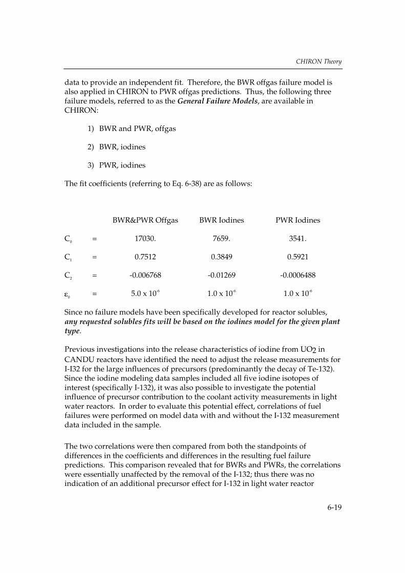
CHIRON Theory
6-19
data to provide an independent fit. Therefore, the BWR offgas failure model isalso applied in CHIRON to PWR offgas predictions. Thus, the following threefailure models, referred to as the General Failure Models, are available inCHIRON:
1) BWR and PWR, offgas
2) BWR, iodines
3) PWR, iodines
The fit coefficients (referring to Eq. 6-38) are as follows:
BWR&PWR Offgas BWR Iodines PWR Iodines
C0 = 17030. 7659. 3541.
C1 = 0.7512 0.3849 0.5921
C2 = -0.006768 -0.01269 -0.0006488
0= 5.0 x 10⁻⁶ 1.0 x 10⁻⁶ 1.0 x 10⁻⁶
Since no failure models have been specifically developed for reactor solubles,any requested solubles fits will be based on the iodines model for the given planttype.
Previous investigations into the release characteristics of iodine from UO2 inCANDU reactors have identified the need to adjust the release measurements forI-I32 for the large influences of precursors (predominantly the decay of Te-132).Since the iodine modeling data samples included all five iodine isotopes ofinterest (specifically I-132), it was also possible to investigate the potentialinfluence of precursor contribution to the coolant activity measurements in lightwater reactors. In order to evaluate this potential effect, correlations of fuelfailures were performed on model data with and without the I-132 measurementdata included in the sample.
The two correlations were then compared from both the standpoints ofdifferences in the coefficients and differences in the resulting fuel failurepredictions. This comparison revealed that for BWRs and PWRs, the correlationswere essentially unaffected by the removal of the I-132; thus there was noindication of an additional precursor effect for I-132 in light water reactor

CHIRON Theory
6-20
coolants samples. A plausible explanation for the lack of noticeable precursoreffects on CHIRON results is that the yield terms used within CHIRON are“equilibrium” values that include precursor decay contributions in the final yieldterm. Since removal of the I-132 from the measured sample leads to increasedstatistical uncertainty and since precursor contributions are implicitly includedin the CHIRON equilibrium values, it is recommended that I-132 be included inthe measurement samples for CHIRON evaluation.
6.1.3 Concentration to Release Rate Conversions
The conversion of measured coolant activity in volumetric concentrations( Ci/cc) to a release rate ( Ci/sec) is sensitive to a number of plant-cycleconfiguration and operational parameters, which are not always accuratelyknown. The purpose of this section is to explain how the internal CHIRONconversions are performed.
Recall from Eq. 6-1 that there are three “loss” terms that must be accounted for inthe conversion: i is the decay constant for isotope i, is the decay constant ofthe cleanup / letdown system, and is the iodine loss associated with the steamflow (BWRs only). The following matrix shows the applicability of the variousterms for BWR and PWR to offgas and iodine.
(X-marks denote that term is included)
BWR Offgas
Iodine X X X
Rx. Sol X X
PWR Offgas X X
Iodine X X
Rx. Sol X X
The following discussion describes the conversions performed by CHIRON:
Beta, if required, is computed in two steps:

CHIRON Theory
6-21
beta =63.0903
(cc/gal)(min/sec)* Flow Rate
gpm* CU Density
g/cc* CUFlowFact
Unitless
1/sec Cool Massg
(Eq. 6-42)
where:
CU Density Coolant density at the cleanup/letdown flow measurementpoint.
CUFlowFact Conversion factor used by CHIRON to convertcleanup/letdown flow input values to gal/min from userspecified unit.
Flow Rate Cleanup/letdown flow rate at and before sampling.
The beta term is subsequently adjusted to account for the efficiency of theremoval system. This removal efficiency is specified in CHIRON as a plant-cycleconfiguration parameter. The iodines (and reactor solubles) are normallyremoved by the cleanup system ion exchange beds for which a removalefficiency may be specified. In the case of PWR offgas the removal efficiency isnormally assumed to be 100% (1.0) for the letdown system. This adjustment isperformed by a simple multiplication:
BetaOG = beta * GasRemEff (Eq. 6-43)
BetaIOD = beta * IodRemEff (Eq. 6-44)
BetaRXS = beta * SolRemEff (Eq. 6-45)

CHIRON Theory
6-22
where:
GasRemEff PWR Gas removal efficiency for the cleanup/letdownsystem.
IodRemEff Iodine removal efficiency for the cleanup/letdown system.
SolRemEff Solubles removal efficiency for the cleanup/letdown system.
Offgas Conversions
If the offgas measurement is inputted as a volumetric activity concentration, aconversion must be carried out to obtain a coolant activity release rate in
Ci/sec. The offgas conversion within CHIRON is reactor type dependent. Thefollowing equations show how CHIRON handles the offgas conversion.
BWR Offgas
ActivityCi/sec
= Input value * OGfactCi/cc
* SJAE GasFlowcc/sec
(Eq. 6-46)
where
Input value User input coolant sample measurement in volumetricconcentration unit.
OGfact Conversion factor used in CHIRON to convert input to Ci/ccfrom user specified volumetric concentration unit.
SJAEGasFlow
Adjusted gas flow at the Steam Jet Air Ejector (SJAE).

CHIRON Theory
6-23
PWR Offgas
ActivityCi/sec =
(Input value * Ogfact) *Ci/cc
Cool Mass *g
(BetaOG +1/sec
i)1/sec
(Eq. 6-47)
Coolant Sample Density1 g/cc
where:
Input value User input coolant sample measurement in volumetricconcentration unit.
OGfact Conversion factor used by CHIRON to convert offgas input toCi/cc from the user specified volumetric concentration unit.
i Decay constant for isotope i.
and the variable BetaOG is as calculated above by Eqs. (6-42) and (6-43). Notethat the coolant sample density is assumed to be equal to 1 g/cc.
Iodine Conversion
The iodine conversion within CHIRON is not reactor type dependent, with asingle exception: the term, iodine carryover with the steam, is set equal to zerofor PWRs. The following equations show how CHIRON handles the iodineconversion.
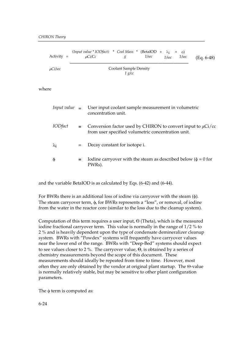
CHIRON Theory
6-24
Activity =(Input value * IODfact)
Ci/Cc* Cool Mass
g* (BetaIOD
1/sec+ i
1/sec+ )
1/sec (Eq. 6-48)
Ci/sec Coolant Sample Density1 g/cc
where
Input value User input coolant sample measurement in volumetricconcentration unit.
IODfact Conversion factor used by CHIRON to convert input to Ci/ccfrom user specified volumetric concentration unit.
i Decay constant for isotope i.
Iodine carryover with the steam as described below ( = 0 forPWRs).
and the variable BetaIOD is as calculated by Eqs. (6-42) and (6-44).
For BWRs there is an additional loss of iodine via carryover with the steam ( ).The steam carryover term, , for BWRs represents a “loss”, or removal, of iodinefrom the water in the reactor core (similar to the loss due to the cleanup system).
Computation of this term requires a user input, (Theta), which is the measurediodine fractional carryover term. This value is normally in the range of 1/2 % to2 % and is heavily dependent upon the type of condensate demineralizer cleanupsystem. BWRs with “Powdex” systems will frequently have carryover valuesnear the lower end of the range. BWRs with “Deep-Bed” systems should expectto see values closer to 2 %. The carryover value, , is obtained by a series ofchemistry measurements beyond the scope of this document. Thesemeasurements should ideally be repeated from time to time. However, mostoften they are only obtained by the vendor at original plant startup. The -valueis normally relatively stable, but may be sensitive to other plant configurationparameters.
The term is computed as:

CHIRON Theory
6-25
= Fraction* StmFlow
lb/hr* [P/Pr]
Fraction(Eq. 6-49)
1/sec Cool Massg
* 7.938(sec/hr) (lb/g)
where:
Theta, the plant-specified fractional steam carryover.
StmFlow Plant Steam Flow in lbs/hr at rated power.
P/Pr Reactor Fractional Power at time of sampling.
The CHIRON equation uses the constant 7.938 to account for proper unitconversion. If the plant ID or configuration specifies a PWR the term is setequal to zero.
Reactor Solubles Conversion
The reactor solubles conversion in CHIRON is not dependent on reactor type.The following equation shows how CHIRON handles the reactor solublesconversion.
Activity =(Input value * RXSfact)
Ci/cc* Cool Mass
g* (BetaRXS
1/sec+ i)
1/sec(Eq. 6-50)
Ci/sec Coolant Sample Density1 g/cc
where:
Input value User input coolant sample measurement in volumetricconcentration unit.
CHIRON Theory
6-26
RXSfact Conversion factor used in CHIRON to convert input to Ci/ccfrom user specified volumetric concentration unit.
i Decay constant for isotope i.
and the variable BetaRXS is as calculated above by Eqs. (6-42) and (6-45).
6.2 COMBINED FAILURE MODEL
The most significant cause of uncertainty of the General Failure Models inCHIRON is the user requirement to input the rod power factor (RPF), i.e., the ratioof the linear heat rating of the failed fuel to the core average linear heat rating. Inseveral cases where CHIRON was unsuccessful in predicting the number offailures correctly, re-analyses were performed after experimental determination ofthe rod power factor of the failed rods, and these analyses proved to beconsiderably more accurate. Therefore, the “Combined Failure Model” wasdeveloped, which uses a special technique to estimate the RPF while the reactor isstill operating, in an attempt to achieve improved failure predictions. Thedevelopment of the “Combined Failure Model” is described in the following.
6.2.1 Existing Improved Method
In some cases it is possible to establish an empirical connection between certainfailure modes and the characteristics of the associated coolant and offgas activities.In a study performed by Taipower (Reference 6), D. Lin reported that frettinginduced failures tended to be associated with larger defect sizes and relatively lowvalues of the activity release rate per failed rod. The latter translates into a low rodpower factor for the failed fuel. Thus, the study essentially establishes an empiricalrelationship between the defect size parameter, , and the rod power factor, for aspecific failure mode. Since the basic CHIRON analysis normally calculates thevalue of , the subsequent failure predictions may be improved for the specificfailure mode by taking advantage of the associated value of the rod power factor.
6.2.2 Improvement Development for CHIRON
Significant improvement of the CHIRON on-line failure predictions could beachieved if the rod power factor can be determined during operation from coolantand offgas activity, without the assumption of a particular failure mode.
Analyses have been performed on a number of recent, well-documented cases offuel failures in both BWRs and PWRs. These analyses, have revealed that it may be

CHIRON Theory
6-27
feasible to determine the rod power factor directly from fission product activitysamples. The fundamental principle that allows this determination is the fact thatthe ratio between the activities associated with the iodines and noble gases from thefailed fuel rod(s) is temperature dependent. This temperature dependency is dueto the difference in the individual temperature dependencies for iodines and noblegases with respect to the migration characteristics through the fuel rod and coresystem. Thus, for the method to be successful, both iodine and offgas samples ofgood quality must be available from within the same time interval. In this context,"good quality" means that both a and can be determined by CHIRON.
6.2.3 Operating Plant Observations
A total of thirteen plant cycles (five BWR and eight PWR)were selected for whichthe following characteristics applied:
1. At least one failure was monitored for sufficient time to establish steady-stateconditions, and no degradation (i.e., fuel particle release) was observedwithin that time period.
2. Dual samples (iodines and offgas) were obtained of sufficient quality to allow"three-coefficient fits" by CHIRON (i.e., the sample analyses allowed thedetermination of both a and ).
3. The actual number of failed rods could be determined from available post-cycle fuel examination data.
4. The average failed rod power factor could be estimated from core loadingand power history information from the plant.
Furthermore, the plant cycles were so selected that several of them were known tohave had only one failure, while a few had shown large numbers of failures.
Three of the plant cycles provided multiple data points due to a stepwise increasein the number of failed rods through the cycle and/or varying power levels of thefailed fuel. In these cases, the intermediate "observed" numbers of failed rods wereinferred from the CHIRON trending plots, using the General Failure Model foroffgas, and proportioning the failure prediction trend to give the correct result atend-of-cycle.
The failed fuel rod power factors were estimated from core loading informationand, where available, failed fuel power histories. In all cases of multiple failures, aweighted average of the failed fuel power was used, giving the highest weight tothe highest powered failed rods. In cases where no specific information on thepower level of the failed fuel was available; the rod power factors were set to unity.

CHIRON Theory
6-28
6.2.4 Data Analysis
According to the CHIRON theory described in Section 6.1, the a-coefficient isproportional to a weighted sum of activity contributions from all the failed rods. Itbasically represents the diffusion rate of the radioactive nuclides through the fuelpellets and the rod free volume, and it includes the functional dependency on thefuel temperature. However, CHIRON does not specifically output the value of "a",because the calculated quantity a is used directly in the failure models. Thus, inthe present analysis the notation "a" always means "a / ", which preserves thedirect connection to the CHIRON-calculated quantities. Notably, this also impliesthat "a" is only available when both is non-zero, i.e., when the sample data allowsa three-coefficient fit.
To facilitate the discussion below, the following terminology is used:
X = The number of failed rods in the core.
a (= a / ) = The total release coefficient for a given isotopic group (iodinesor noble gases).
an (= a/X) = The normalized release coefficient for a given isotopic group(iodines or noble gases).
Offgas = This term is used interchangeably with the term "noble gases".
Since "a" is a sum of contributions from all the failed rods, the normalized releasecoefficient refers to the average release rate per failed rod. Expressed individuallyfor iodines and offgas it becomes:
an,I = aI/X (Eq. 6-51)
an,O = aO/X (Eq. 6-52)
where subscripts I and O refer to iodines and offgas, respectively.
Furthermore, if the dependency of the diffusion coefficient component of an on thefailed rod heat rating (which is also considered a proportional measure oftemperature) is assumed to be exponential, Eqs. 6-51 and 6-52 may be rewritten:
an,I = an0,I * (LHGR/LHGR0) * exp[cI (LHGR-LHGR0)/LHGR0 ] (Eq. 6-53)

CHIRON Theory
6-29
an,O = an0,O * (LHGR/LHGR0) * exp[cO (LHGR-LHGR0)/LHGR0 ] (Eq. 6-54)
where:
an0,I = the normalized release coefficient for iodines at the referenceheat-rating.
an0,O = the normalized release coefficient for noble gases at thereference heat-rating.
cI = coefficient for the power dependency of the diffusional iodinerelease rate from the fuel pellet.
cO = coefficient for the power dependency of the diffusional noblegas release rate from the fuel pellet.
LHGR = the heat rating of the failed fuel.
LHGR0 = a reference heat-rating.
The component of an that shows a linear dependency of LHGR (the second factor ofEqs. 6-53 and 6-54) reflects the magnitude of the fission product generation rate.
Eqs. 6-51 through 6-54 lead to:
aI/aO = A * exp[ B * (LHGR-LHGR0)/LHGR0 ] (Eq. 6-55)
or:
LHGR=LHGR0 ( 1 + ln[( aI/aO)/A ] / B) (Eq. 6-56)
where:
A = an0,I/an0,O (Eq. 6-57)
B = cI - cO (Eq. 6-58)
The number of failed rods may now be expressed by:
X = aI/an0,I *LHGR0/LHGR* exp[ - cI (LHGR-LHGR0)/LHGR0 ] (Eq. 6-59)
and:
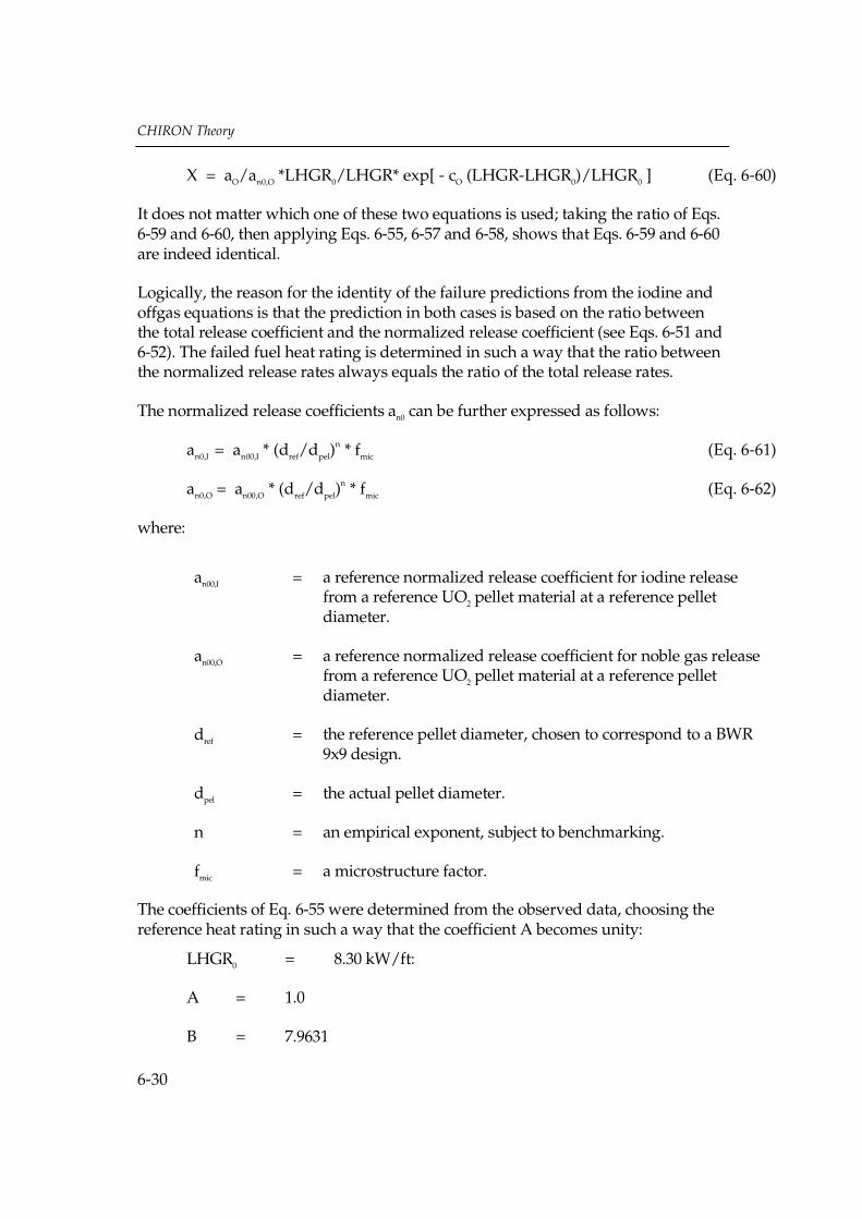
CHIRON Theory
6-30
X = aO/an0,O *LHGR0/LHGR* exp[ - cO (LHGR-LHGR0)/LHGR0 ] (Eq. 6-60)
It does not matter which one of these two equations is used; taking the ratio of Eqs.6-59 and 6-60, then applying Eqs. 6-55, 6-57 and 6-58, shows that Eqs. 6-59 and 6-60are indeed identical.
Logically, the reason for the identity of the failure predictions from the iodine andoffgas equations is that the prediction in both cases is based on the ratio betweenthe total release coefficient and the normalized release coefficient (see Eqs. 6-51 and6-52). The failed fuel heat rating is determined in such a way that the ratio betweenthe normalized release rates always equals the ratio of the total release rates.
The normalized release coefficients an0 can be further expressed as follows:
an0,I = an00,I * (dref/dpel)n * fmic (Eq. 6-61)
an0,O = an00,O * (dref/dpel)n * fmic (Eq. 6-62)
where:
an00,I = a reference normalized release coefficient for iodine releasefrom a reference UO2 pellet material at a reference pelletdiameter.
an00,O = a reference normalized release coefficient for noble gas releasefrom a reference UO2 pellet material at a reference pelletdiameter.
dref = the reference pellet diameter, chosen to correspond to a BWR9x9 design.
dpel = the actual pellet diameter.
n = an empirical exponent, subject to benchmarking.
fmic = a microstructure factor.
The coefficients of Eq. 6-55 were determined from the observed data, choosing thereference heat rating in such a way that the coefficient A becomes unity:
LHGR0 = 8.30 kW/ft:
A = 1.0
B = 7.9631
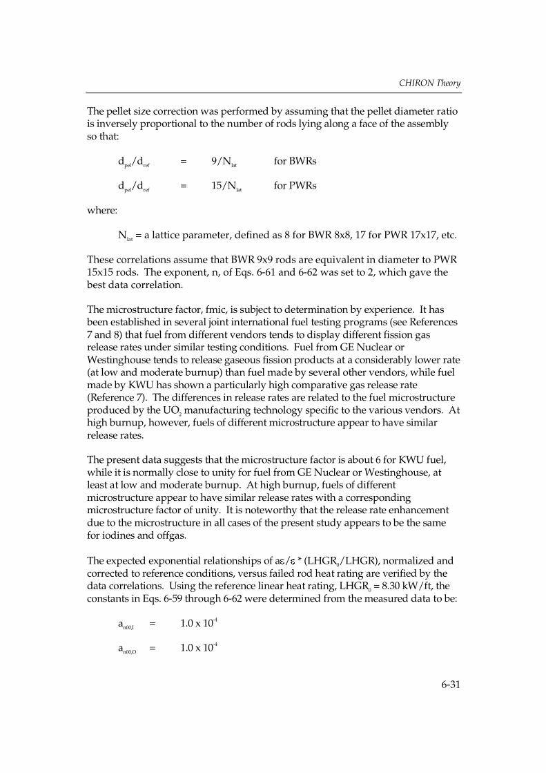
CHIRON Theory
6-31
The pellet size correction was performed by assuming that the pellet diameter ratiois inversely proportional to the number of rods lying along a face of the assemblyso that:
dpel/dref = 9/Nlat for BWRs
dpel/dref = 15/Nlat for PWRs
where:
Nlat = a lattice parameter, defined as 8 for BWR 8x8, 17 for PWR 17x17, etc.
These correlations assume that BWR 9x9 rods are equivalent in diameter to PWR15x15 rods. The exponent, n, of Eqs. 6-61 and 6-62 was set to 2, which gave thebest data correlation.
The microstructure factor, fmic, is subject to determination by experience. It hasbeen established in several joint international fuel testing programs (see References7 and 8) that fuel from different vendors tends to display different fission gasrelease rates under similar testing conditions. Fuel from GE Nuclear orWestinghouse tends to release gaseous fission products at a considerably lower rate(at low and moderate burnup) than fuel made by several other vendors, while fuelmade by KWU has shown a particularly high comparative gas release rate(Reference 7). The differences in release rates are related to the fuel microstructureproduced by the UO2 manufacturing technology specific to the various vendors. Athigh burnup, however, fuels of different microstructure appear to have similarrelease rates.
The present data suggests that the microstructure factor is about 6 for KWU fuel,while it is normally close to unity for fuel from GE Nuclear or Westinghouse, atleast at low and moderate burnup. At high burnup, fuels of differentmicrostructure appear to have similar release rates with a correspondingmicrostructure factor of unity. It is noteworthy that the release rate enhancementdue to the microstructure in all cases of the present study appears to be the samefor iodines and offgas.
The expected exponential relationships of a / * (LHGR0/LHGR), normalized andcorrected to reference conditions, versus failed rod heat rating are verified by thedata correlations. Using the reference linear heat rating, LHGR0 = 8.30 kW/ft, theconstants in Eqs. 6-59 through 6-62 were determined from the measured data to be:
an00,I = 1.0 x 10⁻⁴
an00,O = 1.0 x 10⁻⁴

CHIRON Theory
6-32
cI = 7.1668
cO = -0.7963
Note that the coefficient cO is negative. The release rate of the volatile fissionproducts from a failed fuel rod is governed partly by diffusion in the fuel grains,partly by migration through grain boundaries, cracks and the fuel-cladding gap.The negative sign indicates that the release of the noble gases is limited by the latterprocess. This may be facilitated by the mechanical pressure reduction that followsfrom a temperature (power) reduction.
Eqs. 6-59 and 6-60 are used to determine the number of failed rods, based on theCHIRON-calculated values of a and for iodines and offgas, after the linear heatrating of the failed rods has been determined from Eq. 6-56.
6.2.6 Demonstration of Benchmark Fit to Database
The Combined Failure Model defined in Section 6.2.5.2 was applied to the sameplant cycle case data from which it was developed. The results (predicted failedfuel rod power factor and number of failed rods) are shown in Table 6-2, withcomparison to the experimental values.

CHIRON Theory
6-33
Table 6-2Calculation of Rod Power Factor and Number of Failures from Model
Plant CycleData Point
RPFPredicted
RPFActual
LHRPredicted
kW/ft
N-Fail-Predicted
N-FailActual
BWR-A 1.0 1.0 6.47 1.2 1
BWR-B 0.7 0.7 4.63 0.4 1
BWR-C 1.2 1.2 7.47 0.7 1
BWR-D 1.0 1.0 6.10 1.4 2
BWR-E 0.7 0.7 4.27 1.7 2
PWR-A 0.9 0.9 5.05 4.0 3
PWR-B 1.0 1.0 5.33 1.9 1
PWR-C 0.4 0.4 2.13 9.8 9
PWR-D 0.5 0.4 2.13 33.1 35
PWR-E 0.9 1.0 2.80 0.9 1
PWR-F 0.8 0.9 4.71 7.8 7
PWR-G 1.1 1.0 3.86 19.8 26
PWR-H 1.1 1.2 3.31 70.8 64
CHIRON Theory
6-34
Note that this process merely serves the purpose of checking the internalconsistency of the numerical procedure, as well as illustrating the scatter inherentin the benchmarking database. A validation check against additional, independentdata will be performed at a later time.
Figures 6-1 and 6-2 show the scatter of the fit to the experimental database for rodpower factors and numbers of failed rods, respectively. It is noted that the numberof failures is predicted well within a factor 2 for all but one of the cases. This datapoint was known to be a very small failure. Thus, the activity signals were small,and the measurements subject to particularly large uncertainty.
The scatter of the General Failure Models in CHIRON is such that the number offailures is predicted within a factor of two in 85 % of the cases for BWR offgasanalyses at reactor relative powers higher than 80 %. For BWR iodine analysesand for PWR analyses the scatter of these failure models is greater. The modelsalso contain significant systemic deviations for regimes not fully covered by theoriginal benchmarking. Such regimes are, for instance, low power frettingfailures and all cases for which the reactor was operating at less than 80 % ratedpower.
The Combined Failure Model predicts well within the same scatter band of a factortwo as the General Failure Models. However, contrary to the General FailureModels, the Combined Failure Model may be expected to apply equally well to allconditions, including BWRs and PWRs, offgas and iodine analyses, and all levels ofrelative reactor power. The scatter band is partly due to the scatter in the inputdata, and partly due to crudeness of model assumptions. It can therefore not bereduced below a certain limit, defined by the state-of-the-art of the activity datacollection methods, and the available opportunities for model improvement. Thus,the improvement that the Combined Failure Model represents over the GeneralFailure Models lies largely in the generality of the approach, i.e., its ability toachieve on-line predictions within the acceptable scatter-band of a factor of two inpractically all cases and under all conditions.
The new model offers the advantages of on-line failed fuel power determinationand reconciliation of the predictive models based on iodines and offgas. Theseadvantages are made available as a direct benefit from obtaining simultaneoussamples of both radioactive species. Thus, a significant incentive has beenidentified to obtain synchronous dual sample measurements of both iodine andoffgas activities, for both BWRs and PWRs.

CHIRON Theory
6-35
Figure 6-1Combined Failure Model RPF Comparison

CHIRON Theory
6-36
Figure 6-2Combined Failure Model Failure Comparison

CHIRON Theory
6-37
6.3 CHIRON Fuel Failure Database
An extensive fuel performance database has been accumulated for the purpose ofestablishing reliable fuel failure correlations for both PWR and BWR plant types.The original CHIRON fuel failure database was collected in 1984-1989, andcontains approximately 2000 activity samples from BWRs and PWRs in theUnited States, dating from the period 1972-1988. This database was laterexpanded to include newer samples, mainly from PWRs with incidents ofmultiple failures. This expanded database, last updated in 1992, remains thebasis for the General Failure Models.
The CHIRON database includes iodine and noble gas (offgas) coolantmeasurement results from samples covering a wide range of fuel rod operatingpowers. The data includes a variety of defect types (baffle jet fretting, crud-induced localized corrosion (CILC), pellet-cladding mechanical interaction (PCI),debris-induced failures, etc.) in an attempt to ensure that the resulting failurecorrelations would be applicable to most known defect mechanisms. Sampledata in the database were systematically categorized as being applicable for useas modeling, benchmark, or low power purposes.
Modeling data was used to develop the correlation coefficients for the variouscorrelations at near full power conditions (core power > 95%, rod power factor(RPF) > .9). These samples were selected as being consistent, reliablemeasurements taken during equilibrium conditions near the end of the plant’soperating cycle (in order to ensure that the measurements coincided with thenumber of failures observed after cycle shutdown).
Benchmark data was selected as being typical of in-field measurements. Thesesamples usually contained one or more nuclide readings that, when observed inrelation to the other data, appeared to deviate somewhat from “typical” values,but whose data could not be discarded for known or suspected reasons.Comparison of these data with predictions by the correlations generated fromthe modeling data provided an evaluation of the validity of each correlation.
Low power data was selected on the basis of the same criteria as model data,except that the core and/or rod powers were below the model data acceptancevalues. These samples were used to extend the validity of the correlations intolow power operating domains.
An additional database was started in 1992, to include data from entire reactorcycles, especially such cycles for which severe fuel failures have been detected orsuspected. Severe fuel failures are defined as failures that involve direct release

CHIRON Theory
6-38
of fuel particles from the failed rods. This work was sparked by the EPRI SevereFuel Failures Study for BWRs (Reference 9) and, therefore, the database initiallyfocused on BWR cycles. This database is continually expanding, and nowincludes a large number of PWR cycles. The development of the CombinedFailure Model was based on this expanded database.
6.4 The INPO FRI
The INPO FRI has been implemented in CHIRON according to the June 1992memorandum from INPO (Reference 2), as amended by INPO letter to EPRI ofDecember 1992.
Accordingly, CHIRON calculates single-sample FRI-values, based on theappropriate sample group (offgas for BWRs, iodines for PWRs). At the end of aspecified period, CHIRON then averages the single-sample values, acceptingonly samples that comply with the INPO criteria for steady state and powerlevel. The averaged FRI value is finally groomed to meet the INPO specifiedminimum value for the given reactor type, and/or a maximum value indicatedby the “Sum-of-Six” or “Sum-of-Five”, as applicable, based on monthly averagesof individual, power-corrected isotopic activities. If the selected averagingperiod coincides with a month, the resulting average FRI will be the valuereportable to INPO.

7-1
7 DIAGNOSTICS AND ERROR CHECKING
Chiron generates error messages when a user tries to perform an illegaloperation or tries to enter data that is not in the correct format or outside theacceptable range for that data entry field. A sample of a CHIRON error messageis shown in Figure 7-1.
Figure 7-1Sample CHIRON Error Message
A list of error messages that are generated by CHIRON is provided in thefollowing subsections. The messages have been grouped into three categories:data input errors, database related errors and miscellaneous errors.
7.1 Data Input Error Messages
Data input error messages tell you what data field needs to be corrected andprovides the correct format. Should you encounter a data input error messagewhile using CHIRON, read the message carefully, write it down and then clickon “OK” to return to the data entry field. Correct the data entry using therecommended format and range. Sample error messages are given below.
Diagnostics and Error Checking
7-2
"Chiron cannot set its timer. Please close any open applications and retry."
"The Fit Coefficient model value was not correct"
"The Failure model value was not correct"
"Select a sample for editing"
"The following values are not within acceptable ranges: ... Please correct thesevalues. A list of acceptable ranges can be found in the CHIRON User's Manual."
"Invalid string! Please enter another string, making sure that it has no more than7 characters and does not contain any white spaces or illegal characters such as *,?, /, and =. "
"Start date is earlier than date of first sample; please re-select."
"End date is later than date of last sample; please re-select."
"Start date is later than end date; please re-select."
"Cannot clear selections in SHOW SELECTED SAMPLES ONLY mode"
" The CalcDays sample number is out of range"
"The sample index is > the lastone!"
"Some negative data is on a LOG plot, the graphing is Aborted!"
"The plant is a PWR. All data in the BWR-specific block will be ignored."
"The plant type has changed. Are you sure?"
"Plant/cycle id is limited to 8 characters"
"You must select at least one cycle from the list."
"There is no sample data in the database. To enter sample data for anyplant/cycle in the database, please choose Data | New. If you have not yetentered plant/cycle data, please first select Options | Plant Config | Add NewPlant."
"Plant does not exist in the database. You may add a new plant from the mainmenu."

Diagnostics and Error Checking
7-3
"This sample has been added to the database. Do you wish to add anothersample?"
"The graph_index is not correct, please re-select"
"Out of range value for select_index (expected an integer from 0 to 85)"
"Error: Couldn't find plant/cycle corresponding to this sample. Aborting range-check function."
"Date format must be mm/dd/yy. Valid dates range from 01/01/70 (January 1,1970) to 02/05/36 (February 5, 2036)."
"Time format must be hh:mm:ss in 24-hour format. For example, 4:03 p.m. and22 seconds would be 16:03:22, and midnight would be 00:00:00."
"Plant Id must be of the form Plantname-cycle, e.g. Hatch1-1"
"The fuel type must be of the form NxN or NNxNN. Examples: 8x8 or 15x15."
"This sample will not be added to the database because at least one value isoutside of its acceptable range. Please see the CHIRON User's Manual for alisting of acceptable ranges."
"An error occurred at value number %d."
"No samples were added to the database."
"Cannot delete batch because a batch is not currently selected. You may select asample as part of a batch by double-clicking on it, or by highlighting it andpressing ‘Toggle Status’. Or you may select a batch using ‘Time-Select Batch’. "
"Select a sample for viewing"
"Select a sample for update"
"Cannot analyze batch because a batch is not currently selected. You may selecta sample as part of a batch by double-clicking on it, or by highlighting it andpressing ‘Toggle Status’. Or you may select a batch using ‘Time-Select Batch’. "
"%d samples were selected, which exceeds the %d sample limit. Cannot performtrend plots."

Diagnostics and Error Checking
7-4
7.2 Database Related Error Messages
Database related error messages generally mean you have performed an illegaloperation. Should you encounter a database related error message while usingCHIRON, read the message carefully, write it down and then click on “OK” toreturn to the program. Sometimes database related error messages provide asolution to the problem in the message, and sometimes they do not. If nosolution is given, exit from CHIRON and then open the program again. Sampleerror messages are given below.
"The Selected Sample query in BATCH:pSampleSet failed!"
"The Sample queried in BATCH: doesn't match!"
"The Sample ASCII dump in BATCH: failed!"
"The Requery_Plant_Record in BATCH failed!"
"The PlantDataSet Query in BATCH failed"
"The Plant ASCII dump in BATCH: failed!"
"The RequeryRecord in BATCH:FailureSet failed!"
"Can't Update BATCH pFailureSet!"
"The AddNew_Record in BATCH:pFailureSet failed!"
"The New Edit in BATCH:pFailureSet failed!"
"The pFailureSet CanUpdate failed!"
"The pFailureSet Update failed!"
"The Update in BATCH:pFailureSet failed!"
"The Activity ASCII dump in BATCH: failed!"
The FitFailures ASCII dump in BATCH: failed!"
"Cannot open file"
"Reopened last active datasource."

Diagnostics and Error Checking
7-5
"Cannot reopen current Datasource. Application will terminate."
"Database access error. Application will terminate."
"CChironCalc::unit_conversion, SampleUnits Failed"
"m_pFailureSet->Close() failed."
"m_pFailureSet->Open() failed."
"m_pFailureSet->MoveFirst() failed."
"m_pFailureSet->Edit() failed."
"m_pFailureSet->Update() failed."
"m_pFailureSet->MoveNext() failed."
"Error: Found multiple records corresponding to this sample in the failurestable."
"Error while updating sample data. Changes were not accepted."
"Error on SampleSet Requery"
"This function is not available in the SHOW SELECTED SAMPLES ONLY mode"
"The highlighted sample will be permanently deleted from the database.Proceed with sample deletion?"
"Sample Deletion, bad index"
"The selected (X-marked) samples will be permanently deleted from thedatabase. Proceed with sample deletion? "
"m_pFailureSet->Requery() failed."
"DeleteItem: The Cursor selection is invalid"
"Selection status cannot be changed in SHOW SELECTED SAMPLES ONLYmode"
"Cannot display selected samples because no samples are selected for batchanalysis."

Diagnostics and Error Checking
7-6
"Select a sample for analysis"
"The Selected Sample query in VIEW:pSampleSet failed!"
"The Sample queried in VIEW: doesn't match!"
"The Open_Plant_Record in VIEW:pPlantDataSet failed!"
"The PlantDataSet Query failed"
"The Open_Record in VIEW:FailureSet failed!"
"Can't Update pFailureSet!"
"The AddNew_Record in VIEW:pFailureSet failed!"
"The New Edit in VIEW:pFailureSet failed!"
"The Update in VIEW:pFailureSet failed!"
"The Open FailureRecord in TREND failed!"
"%d samples were selected, which exceeds the %d sample limit. Cannot performbatch analysis."
"The ASCII dump files already exist. Overwrite the old files?"
"The Open PlantRecord in BATCH failed!"
"The Open FailureRecord in BATCH failed!"
"FindSampleRange error"
"SetSelectListBoxItems function failed!"
"CHIRON could not launch the selected text editor. You may open the QAreport file (qareport.txt) in any available editor outside of CHIRON."
"An error occurred. The QA Report was not written."
"The QA Report has been saved as 'qareport.txt'."
"PEcreate failed"
"Graph properties failed"

Diagnostics and Error Checking
7-7
"Graph creation failed"
"m_pFlagFailureSet->Close() failed."
"m_pFlagFailureSet->Open() failed."
"m_pFlagFailureSet->MoveFirst() failed."
"m_pFlagFailureSet->Edit() failed."
"m_pFlagFailureSet->Update() failed."
"m_pFlagFailureSet->MoveNext() failed."
"m_pFailureSet->Requery() failed in Ctrendgraph::SelectBuffer!"
7.3 Miscellaneous Error Messages
Miscellaneous error messages generally relate to system errors. Should youencounter a miscellaneous error message while using CHIRON, read themessage carefully, write it down and then click on “OK” to return to theprogram. You may need to exit CHIRON and restart the program. A list ofmiscellaneous error messages is given below.
"Calculation information: Calculated FRI is greater than sum of 6. See CHIRONUser's Manual for more information." (This is an information message only. Itidentifies the type of calculation being used for the FRI computation. No useraction is required other than clicking “OK” and continuing with CHIRONprocessing.)
"A memory exception occurred during Compare String processing!" (This is aninternal error message indicating that memory available to the operating systemis not sufficient to continue CHIRON execution. It may be necessary to exitCHIRON and reboot the computer system.)
"Memory allocation error. Application will terminate" (This is an internal errormessage indicating that memory available to the operating system is notsufficient to continue CHIRON execution. It may be necessary to exit CHIRONand reboot the computer system.)
"SetGraph_Properties bad m_hPE" (This is a graphical system internal errormessage that should not be encountered during normal CHIRON operation. Ifthis message occurs, the user should notify CHIRON Technical Support.)

Diagnostics and Error Checking
7-8
"Graphdlg:Set_Subsetpts bad graph type" (This is a graphical system internalerror message that should not be encountered during normal CHIRONoperation. If this message occurs, the user should notify CHIRON TechnicalSupport.)

8-1
8 REFERENCES
1. CHIRON - A Fuel Failure Prediction Code. Revised User’s Manual for Version 2.1,EPRI TR-102297, July 1993.
2. “Fuel Reliability,” Enclosure to Memorandum from Institute for Nuclear PowerOperations to Electric Power Research Institute, June 1992.
3. An Improved Failure Model for Use in the Fuel Failure Prediction Code CHIRON.October 1995, to be published as EPRI Report.
4. A.H. Booth, “A Suggested Method for Calculating the Diffusion of RadioactiveRare Gas Fission Products from UO2 Fuel Elements and a Discussion ofProposed In-Reactor Experiments That May Be Used to Test Its Validity,” AE-700, 1957, Atomic Energy of Canada, Ltd.
5. B.J. Lewis, “A Model for the Release of Radioactive Krypton, Xenon, and Iodinefrom Defective UO2 Fuel Elements,” Nuclear Technology, Vol. 73, April 1986.
6. David Lin, "An Improved Model for Estimating the Number and Size ofDefected Fuel Rods in an Operating Reactor," ANS/IAEA Topical Meeting onLight Water Reactor Fuel Performance, April 17-21, 1994.
7. The SUPER-RAMP Project. Final Report, STUDSVIK-STSR-32, StudsvikNuclear: December 1984.
8. The Third Risø Fission Gas Release Project. RISØ-FGP3-FINAL, Part 1, RisøNational Laboratory: March 1991.
9. Severe Degradation of BWR Fuel Failures: Coolant Activity Analysis, EPRITR-102799, November 1993.

References
8-2

A-1
A LIST OF FILES INSTALLED BY CHIRON
Below is the listing of the files that are installed on your computer system duringthe CHIRON installation procedure. The location listed in the table is the defaultlocation. If you follow the installation as described in Section 2 of this manualand use the default directory, this is where the files will be placed on yoursystem.
File Name Version Location Size(Bytes)
Purpose
Ctl3dv2.dll 2.31.0.00 C:\WINDOWS\SYSTEM 27,632 ODBC File
12510866.cpx C:\WINDOWS\SYSTEM 2,318 ODBC File
12520437.cpx C:\WINDOWS\SYSTEM 2,151 ODBC File
12520850.cpx C:\WINDOWS\SYSTEM 2,233 ODBC File
12520860.cpx C:\WINDOWS\SYSTEM 2,167 ODBC File
12520861.cpx C:\WINDOWS\SYSTEM 2,162 ODBC File
12520863.cpx C:\WINDOWS\SYSTEM 2,173 ODBC File
12520865.cpx C:\WINDOWS\SYSTEM 2,147 ODBC File
Cpn16ut.dll C:\WINDOWS\SYSTEM 3,264 ODBC File
12500852.cpx C:\WINDOWS\SYSTEM 2,320 ODBC File
Odbc16ut.dll C:\WINDOWS\SYSTEM 5,792 ODBC File
Drvssrvr.hlp C:\WINDOWS\SYSTEM 105,964 ODBC File

CHIRON Database Format
A-2
File Name Version Location Size(Bytes)
Purpose
Msajt200.dll 2.50.0.1606 C:\WINDOWS\SYSTEM 995,136 ODBC File
Mscpxlt.dll 2.0.19.12 C:\WINDOWS\SYSTEM 10,304 ODBC File
Msjetdsp.dll 1.10.0.1 C:\WINDOWS\SYSTEM 85,792 ODBC File
Msjeterr.dll 2.50.0.1111 C:\WINDOWS\SYSTEM 11,232 ODBC File
Msjetint.dll 2.50.0.1111 C:\WINDOWS\SYSTEM 15,936 ODBC File
Mstx2016.dll 2.50.0.1117 C:\WINDOWS\SYSTEM 102,080 ODBC File
Msxl2016.dll 2.50.0.1117 C:\WINDOWS\SYSTEM 149,344 ODBC File
Odbc.dll 2.10.24.1 C:\WINDOWS\SYSTEM 56,240 ODBC File
Odbc.inf C:\WINDOWS\SYSTEM 16,584 ODBC File
Dbnmp3.dll 1994.1.26.0 C:\WINDOWS\SYSTEM 10,944 ODBC File
Odbcstp.exe 2.0.20.16 C:\WINDOWS\SYSTEM 72,896 ODBC File
Odbc3216.dll C:\WINDOWS\SYSTEM 12,288 ODBC File
Odbcadm.exe 2.10.23.9 C:\WINDOWS\SYSTEM 6,464 ODBC File
Odbccp32.dll C:\WINDOWS\SYSTEM 5,632 ODBC File
Odbccurs.dll 2.10.23.23 C:\WINDOWS\SYSTEM 88,896 ODBC File
Odbcinst.dll 2.10.24.1 C:\WINDOWS\SYSTEM 92,576 ODBC File
Odbcjet.hlp C:\WINDOWS\SYSTEM 113,064 ODBC File
Odbcjt16.dll 2.0.23.17 C:\WINDOWS\SYSTEM 246,928 ODBC File
Odbcjtnw.hlp C:\WINDOWS\SYSTEM 83,833 ODBC File
Odbc32.dll C:\WINDOWS\SYSTEM 12,800 ODBC File
Vbar2.dll 2.0.0.2420 C:\WINDOWS\SYSTEM 298,880 ODBC File
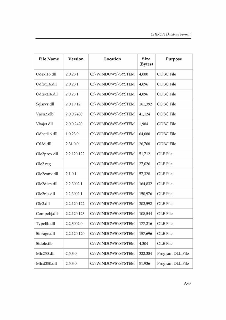
CHIRON Database Format
A-3
File Name Version Location Size(Bytes)
Purpose
Odexl16.dll 2.0.23.1 C:\WINDOWS\SYSTEM 4,080 ODBC File
Odfox16.dll 2.0.23.1 C:\WINDOWS\SYSTEM 4,096 ODBC File
Odtext16.dll 2.0.23.1 C:\WINDOWS\SYSTEM 4,096 ODBC File
Sqlsrvr.dll 2.0.19.12 C:\WINDOWS\SYSTEM 161,392 ODBC File
Vaen2.olb 2.0.0.2430 C:\WINDOWS\SYSTEM 41,124 ODBC File
Vbajet.dll 2.0.0.2420 C:\WINDOWS\SYSTEM 1,984 ODBC File
Odbctl16.dll 1.0.23.9 C:\WINDOWS\SYSTEM 64,080 ODBC File
Ctl3d.dll 2.31.0.0 C:\WINDOWS\SYSTEM 26,768 ODBC File
Ole2prox.dll 2.2.120.122 C:\WINDOWS\SYSTEM 51,712 OLE File
Ole2.reg C:\WINDOWS\SYSTEM 27,026 OLE File
Ole2conv.dll 2.1.0.1 C:\WINDOWS\SYSTEM 57,328 OLE File
Ole2disp.dll 2.2.3002.1 C:\WINDOWS\SYSTEM 164,832 OLE File
Ole2nls.dll 2.2.3002.1 C:\WINDOWS\SYSTEM 150,976 OLE File
Ole2.dll 2.2.120.122 C:\WINDOWS\SYSTEM 302,592 OLE File
Compobj.dll 2.2.120.123 C:\WINDOWS\SYSTEM 108,544 OLE File
Typelib.dll 2.2.3002.0 C:\WINDOWS\SYSTEM 177,216 OLE File
Storage.dll 2.2.120.120 C:\WINDOWS\SYSTEM 157,696 OLE File
Stdole.tlb C:\WINDOWS\SYSTEM 4,304 OLE File
Mfc250.dll 2.5.3.0 C:\WINDOWS\SYSTEM 322,384 Program DLL File
Mfcd250.dll 2.5.3.0 C:\WINDOWS\SYSTEM 51,936 Program DLL File

CHIRON Database Format
A-4
File Name Version Location Size(Bytes)
Purpose
Mfcoleui.dll 2.0.1.0 C:\WINDOWS\SYSTEM 146,976 Program DLL File
Pegraphs.dll 2.0.0.0 C:\WINDOWS\SYSTEM 612,352 Program DLL File
Pegraphs.hlp C:\WINDOWS\SYSTEM 55.846 Program DLL File
Chiron1.exe C:\CHIRON30 565,664 Program File
Dbconv.exe C:\CHIRON30 32,334 Program File
Readme.txt C:\CHIRON30 4,682 Program File
Chiblank.mdb C:\CHIRON30 196,608 Database File
Chiron1.mdb C:\CHIRON30 294,912 Database File
Chiron2.mdb C:\CHIRON30 524,288 Database File
Chiron3.mdb C:\CHIRON30 327,680 Database File
Dbcon090.csv C:\CHIRON30 20,352 Example File
Dbcon091.csv C:\CHIRON30 20,345 Example File
Dbcon092.csv C:\CHIRON30 25,352 Example File
Dbcon093.csv C:\CHIRON30 25,396 Example File
Dbcon094.csv C:\CHIRON30 19.804 Example File
Dbcon095.csv C:\CHIRON30 27,723 Example File
Dbcon09.txt C:\CHIRON30 45,294 Example File
Dbqa.txt C:\CHIRON30 2,579 Example File
Uninst.isu C:\CHIRON30 Uninstall File
Isun16.exe 5.00.219.0 C:\WINDOWS 358,076 Uninstall Program

B-1
B FORMAT OF “FILE READ” ASCII FILE
In order for a file to be read into CHIRON as described in the “File Read” inputoption (see Section 3.3.2 of this manual) it must follow the format presented inthis appendix. Sample data input files created by the database conversionprogram DBConvert are automatically in this format. An example of such a file,File “dbcon09.txt”, is included with the distribution.
If data input files need to be created independently of the database conversionprogram, set up the sample data in a spreadsheet, then export the spreadsheetfile into an ASCII file, using the “comma-separated-values” (CSV) format option.
The File Read ASCII file format includes the following:
Comment lines are allowed anywhere, as denoted by a #-sign in the first column,e. g.:
# File Read file: "<file name>"## ASCII File Read for CHIRON Version 3.0 for WINDOWS; July 1996## Plant ID: DBCON; Cycle: 9## Plant, Cycle, Time, Rx Pow, CU Flow, RPF, BU, OgDelay, IoDelay, -, -, -
where the last comment line can be a listing of all the field headings.
Blank lines are allowed anywhere.
The following fields must be present in each line, separated by commas:
Plant-ID (five-char string)Cycle (one or two digit integer)Date (mm/dd/yy)Time (hh:mm:ss)Rx PowerCU FlowRPF

Format of “File-Read” ASCII File
B-2
BUOgDelayIoDelaySolDelaySJAE FlowXe-138Xe-135mKr-87Kr-88Kr-85mXe-135Xe-133I-134I-132I-135I-133I-131
Tc-101Ba-141Cs-138Ba-139Sr-92Tc-99mSr-91Np-239Mo-99Te-132Ba-140Te-129mSr-89Cs-134Sr-90Cs-137N-13Rb-89Nb-97Ar-41Cu-64Na-24Zr-97Y-90Cr-51Fe-59Hf-181

Format of “File-Read” ASCII File
B-3
Zr-95Co-58Zn-65Mn-54Co-60
All fields in this list which are not specifically type-designated, are numeric. Anynumeric format may be used. Numeric fields must be written in acompacted manner, without embedded blanks (e.g. “3.879e-005”, not “3.879e -5”). However, leading and trailing blanks before or after commas arepermitted.
The total length of a line must not exceed 512 characters.
The regular boldfaced fields are required. If some activities are not available,zeros must be entered.
The italic boldfaced fields are optional.

Format of “File-Read” ASCII File
B-4

C-1
C SAMPLE QA FILE REPORT
The sample analysis QA report provides all input and output data for the currentsingle-sample analysis, including plant configuration data, model parameterselections, calculational options settings, model versions and model constants.This file is intended to provide a complete QA record for any single sample. Forinstructions on how to generate this report, see Section 4.3.8.
A sample QA file report is presented below. This report was produced usingCHIRON and Notepad, a text editor supplied with Windows.

Sample QA File Report
C-2
CHIRON for Windows QA Report for Sample Analysis.
Electric Power Research Institute
Filename: qareport.txt
Plant Cycle, Date, and Time analyzed:
plantcycle BWR02-11
sample date and time 08/12/95 20:30:00
Analysis datetime 03/05/98 17:44:09
Model revisions:
Chiron for Windows Program Rev 3.0 Date 03/01/98
Combined Failure Model Rev 1.1 Date 10/30/95
General Failure Model Rev 2.1 Date 03/15/92
3 Coefficient Fit (2 if epsilon is small) Rev 1.1 Date 03/01/92
INPO FRI Calculation Rev 2.0 Date 12/15/92
Model settings:
Combined Failure flag = TRUE
INPO_FRI_Calculation flag = TRUE
Perform Solubles calculation = FALSE
converg criter 0.0001
epsilon_0 1e-006
f_micro 1
loop on Pu239 fuel yld frac TRUE
fuel Pu239 yld frac 0
converg iterat 50
set Pu239 tramp yld frac FALSE
tramp Pu239 yld frac 0
tramp recoil 1
Sample Input Settings:
Reactor Power 1 %P
Cleanup Flow 200 Gal/min (*)
Rod Power Factor 1
Burnup 0 MWd/kgU (*)
Gas Delay Time 265 (sec)
Iod Delay Time 0 (sec)
Sol Delay Time 0 (sec)
SJAE gas flow 7200 cc/sec (*)

Sample QA File Report
C-3
Xe138 2777 uCi/sec (*)
Xe135M 0 uCi/sec (*)
Kr87 727 uCi/sec (*)
Kr88 731 uCi/sec (*)
Kr85M 247 uCi/sec (*)
Xe135 970 uCi/sec (*)
Xe133 520 uCi/sec (*)
I134 0.002834 uCi/cc (*)
I132 0.001027 uCi/cc (*)
I135 0.0005693 uCi/cc (*)
I133 0.0003094 uCi/cc (*)
I131 8.844e-005 uCi/cc (*)
Tc101 0 uCi/cc (*)
Ba141 0 uCi/cc (*)
Cs138 0.0009035 uCi/cc (*)
Ba139 0.0006686 uCi/cc (*)
Sr92 0.0005708 uCi/cc (*)
Tc99M 6.348e-005 uCi/cc (*)
Sr91 0.0003086 uCi/cc (*)
Np239 0 uCi/cc (*)
Mo99 0 uCi/cc (*)
Te132 0 uCi/cc (*)
Ba140 0 uCi/cc (*)
Te129M 0 uCi/cc (*)
Sr89 0 uCi/cc (*)
Cs134 4.522e-005 uCi/cc (*)
Sr90 0 uCi/cc (*)
Cs137 4.125e-005 uCi/cc (*)
N13 0 uCi/cc (*)
Rb89 0 uCi/cc (*)
Nb97 0 uCi/cc (*)
Ar41 0 uCi/cc (*)
Cu64 0 uCi/cc (*)
Na24 0 uCi/cc (*)
Zr97 0 uCi/cc (*)
Y90 0 uCi/cc (*)

Sample QA File Report
C-4
Cr51 0 uCi/cc (*)
Fe59 0 uCi/cc (*)
Hf181 0 uCi/cc (*)
Zr95 0 uCi/cc (*)
Co58 0 uCi/cc (*)
Zn65 0 uCi/cc (*)
Mn54 0 uCi/cc (*)
Co60 0 uCi/cc (*)
Plant Input Settings:
Rx Type BWR
Rated Power 2436 MW
Rx Water Mass 1.656e+008 g
ClnUp Flow den 1 g/cc
Offgas Rem Eff 1
Iodine Rem Eff 1
Solubl Rem Eff 1
carryover (BWR) 0.003
steamflow (BWR) 1e+007 lbs/hr
number rods 34720
Number bundles 560
rods per face 8
Fuel Length 350.3 cm

Sample QA File Report
C-5
Offgas Isotopes:
Activity Measured and Predicted units: uCi/sec (*)
Xe138 meas 3445.18 pred 7211.23
Xe135M meas 0 pred 1250.9
Kr87 meas 756.881 pred 681.729
Kr88 meas 744.442 pred 654.089
Kr85M meas 249.829 pred 213.51
Xe135 meas 975.413 pred 1053.16
Xe133 meas 520.209 pred 520.02
Release to Birth Measured and Predicted
Xe138 meas 0.00117407 pred 0.00245749
Xe135M meas 0 pred 0.00246257
Kr87 meas 0.00356714 pred 0.00321295
Kr88 meas 0.00550602 pred 0.00483775
Kr85M meas 0.00803281 pred 0.00686502
Xe135 meas 0.0117629 pred 0.0127005
Xe133 meas 0.0859042 pred 0.085873
Iodine Isotopes:
Activity Measured and Predicted units: uCi/sec (*)
I134 meas 149.531 pred 60.4012
I132 meas 31.1703 pred 20.4492
I135 meas 12.0916 pred 17.7368
I133 meas 5.54763 pred 10.4631
I131 meas 1.46479 pred 1.39089
Release to Birth Measured and Predicted
I134 meas 0.000152569 pred 6.16288e-005
I132 meas 0.000147424 pred 9.6717e-005
I135 meas 0.000111388 pred 0.000163391
I133 meas 0.000150392 pred 0.000283646
I131 meas 0.000864266 pred 0.000820661
Solubles Isotopes:
Activity Measured and Predicted units: uCi/sec (*)
Solubles were not performed.
Release to Birth Measured and Predicted
Solubles were not performed.

Sample QA File Report
C-6
Isotope Ratios:
RatioName Activity Ratios Measured Predicted
I131/I133 0.264039 0.132933
I131/I134 0.00979593 0.0230275
I133/I134 0.0371003 0.173227
Xe133/Xe138 0.150996 0.0721125
I131/Xe133 0.00281578 0.00267468
Cs134/Cs137 NA
Sr92/Sr91 NA
Fit and General Failure Model Summary for Offgas:
AEpsilon 1.7045e-009
Epsilon 1.50591e-005
C 0.00238538
R(squared) 0.998619
Convg Err 5.50767e-005
num iterat 13
fit OK TRUE
U235frac 0.89603
Pu239frac 0.10397
Failures 3.84223
Fit and General Failure Model Summary for Iodine:
AEpsilon 7.2868e-013
Epsilon 0
C 0.000132638
R(squared) 0.995829
Convg Err 6.76856e-005
num iterat 9
fit OK TRUE
U235frac 0.944643
Pu239frac 0.0553566
Failures 2.61836
Fit and General Failure Model Summary for Solubles:
Solubles were not performed.
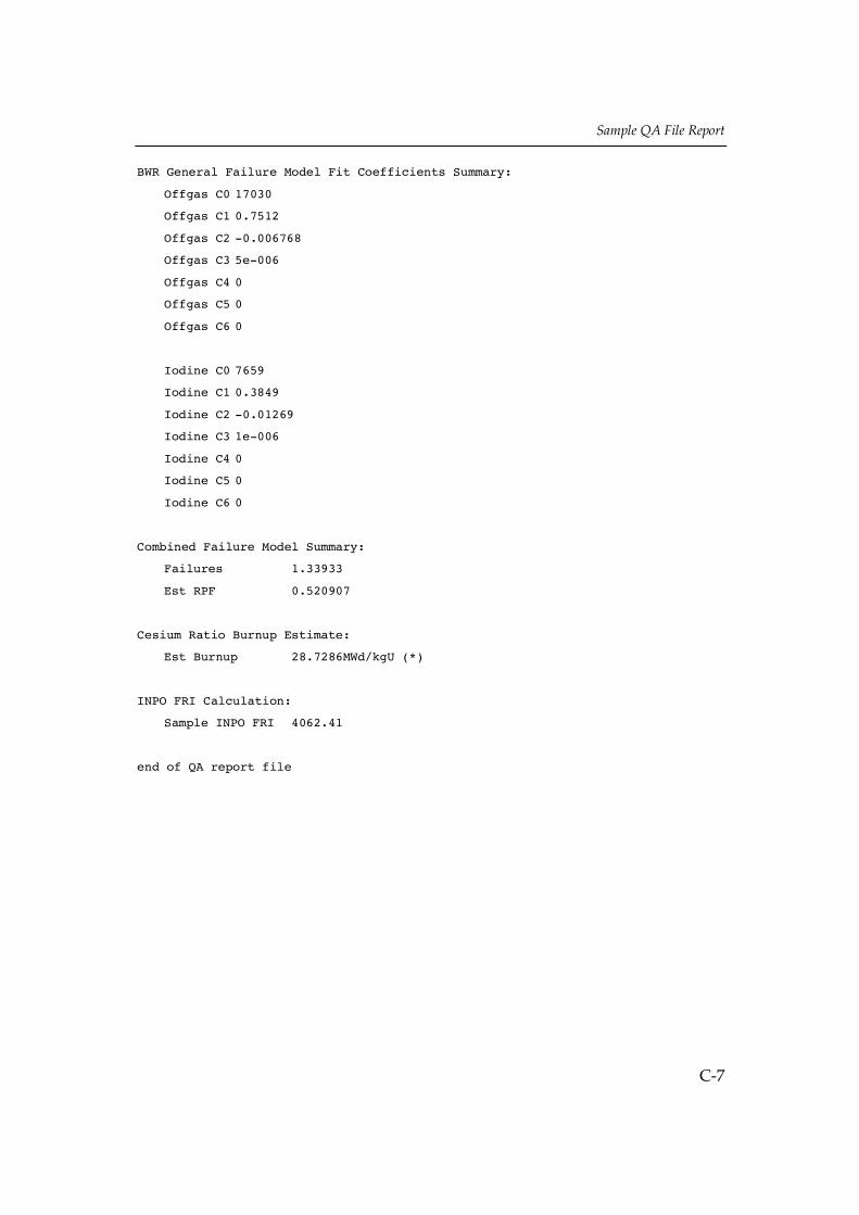
Sample QA File Report
C-7
BWR General Failure Model Fit Coefficients Summary:
Offgas C0 17030
Offgas C1 0.7512
Offgas C2 -0.006768
Offgas C3 5e-006
Offgas C4 0
Offgas C5 0
Offgas C6 0
Iodine C0 7659
Iodine C1 0.3849
Iodine C2 -0.01269
Iodine C3 1e-006
Iodine C4 0
Iodine C5 0
Iodine C6 0
Combined Failure Model Summary:
Failures 1.33933
Est RPF 0.520907
Cesium Ratio Burnup Estimate:
Est Burnup 28.7286MWd/kgU (*)
INPO FRI Calculation:
Sample INPO FRI 4062.41
end of QA report file

Sample QA File Report
C-8

D-1
D ASCII DUMP FILES
Data may be exported from CHIRON by means of the ASCII Dump option. Itgenerates a set of files (ten in all). These files may be read directly into commonspreadsheet applications, such as Microsoft Excel. The sample ASCII Dump filesdisplayed in the remaining pages of this appendix are named Chirond0.txt,Chirond1.txt, etc. through Chirond9.txt.
File “chirond0.txt” contains one row showing the file-name, then a blank row,then one row with column headings, then a blank row, then one row of data perplant-cycle in the batch, then a blank row, and finally a row with an end-of-filesequence.
Files “chirond1.txt” - “chirond9.txt” each contain one row showing the file-name,then a blank row, then one row with column headings, then a blank row, thenone row of data per sample in the batch analysis, then a blank row, and finally arow with an end-of-file sequence.
All column headings and data items are delimited by tabs, thus making the filesreadily available for importing into a spreadsheet application.
D.1 ASCII Dump File “Chirond0.txt”
This file contains plant-cycle information and batch analysis model settings, inthe following format:
Field 1 Plant-cycle IDField 2 Reactor rated power (MWth)Field 3 Number of fuel assemblies in the coreField 4 Active fuel length (cm)Field 5 Water mass in core primary loop (g)Field 6 Failed fuel type (“9x9”, “16x16”, etc.)Field 7 Cleanup/letdown flow density (g/cc)Field 8 OG removal efficiency

ASCII Dump Files
D-2
Field 9 IO removal efficiencyField 10 Solubles removal efficiencyField 11 Iodines carry-over fractionField 12 Steam flow (lbs/hr)Field 13 Reactor type (0 for BWR, 1 for PWR)Field 14 Least squares fit convergence limitField 15 Pu239 fission yield ratio to use when Field 18 is 0.Field 16 Epsilon_0 (default epsilon for Combined Failure Model)Field 17 f_micro (fuel microstructure descriptor, 1 for “normal”, >1 for
AUC type)Field 18 Fission yield (Pu239 fission yield ratio) loop flag (1 for loop, 0 for no
loop)Field 19 Maximum number of iteration loopsField 20 Total number of fuel rods in the coreField 21 Number of rods per face in fuel rod lattice of failed fuel assemblyField 22 Flag to set the Pu239 yield ratio for tramp equal to value for fuel (0
= set to fuel value, 1 = use value from Field 23)Field 23 Pu239 yield ratio for tramp, when not set equal to value for fuelField 24 Fraction of tramp that emits fission products as direct recoi l
D.2 ASCII Dump File “Chirond1.txt”
This file contains sample-specific operational data, in the following format:
Field 1 Plant-cycle IDField 2 Sample dateField 3 Sample timeField 4 Reactor relative power at sample timeField 5 Rod power factor for failed fuel (inputted value)Field 6 Cleanup/letdown flow (gal/min)Field 7 Offgas delay time (seconds)Field 8 Iodines delay time (seconds)Field 9 Solubles delay time (seconds)Field 10 SJAE gas flow (cc/second)Field 11 Failed fuel burnup (MWd/kgU, from inputted value)
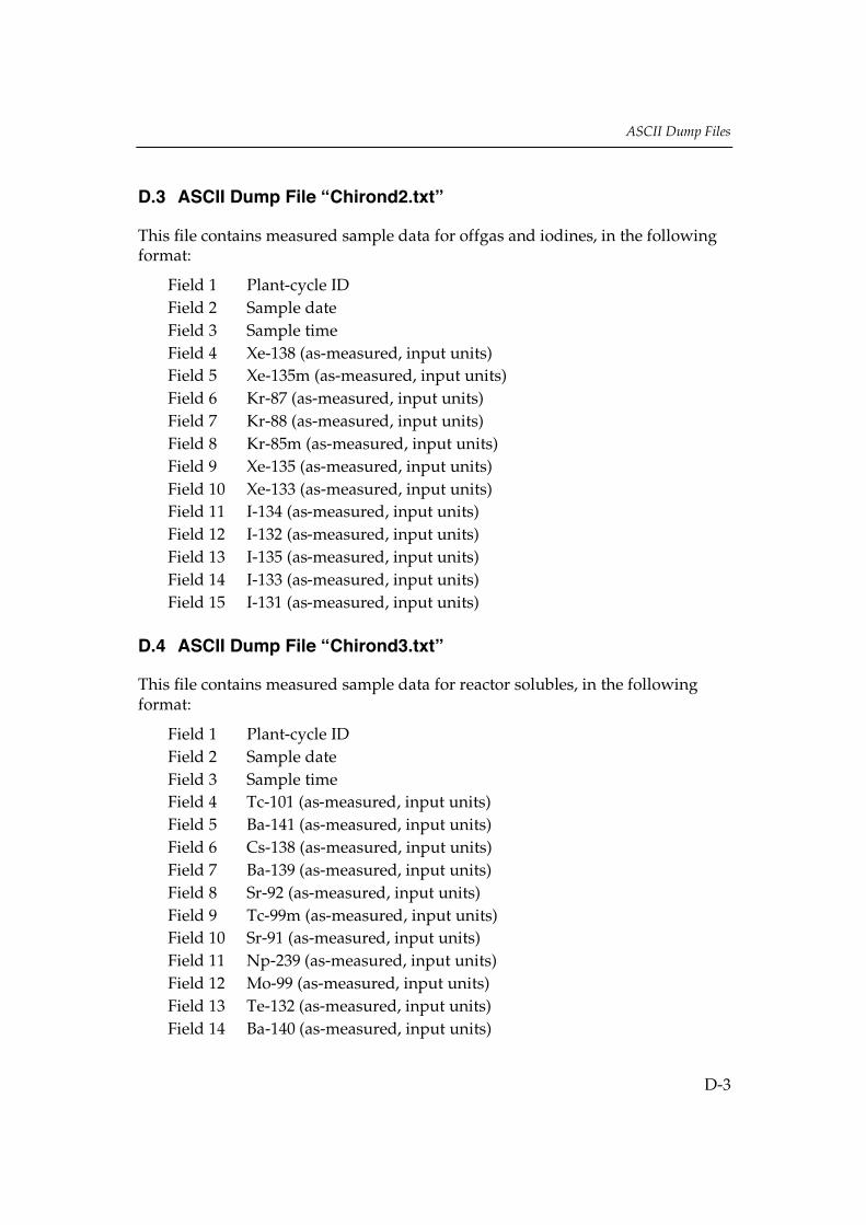
ASCII Dump Files
D-3
D.3 ASCII Dump File “Chirond2.txt”
This file contains measured sample data for offgas and iodines, in the followingformat:
Field 1 Plant-cycle IDField 2 Sample dateField 3 Sample timeField 4 Xe-138 (as-measured, input units)Field 5 Xe-135m (as-measured, input units)Field 6 Kr-87 (as-measured, input units)Field 7 Kr-88 (as-measured, input units)Field 8 Kr-85m (as-measured, input units)Field 9 Xe-135 (as-measured, input units)Field 10 Xe-133 (as-measured, input units)Field 11 I-134 (as-measured, input units)Field 12 I-132 (as-measured, input units)Field 13 I-135 (as-measured, input units)Field 14 I-133 (as-measured, input units)Field 15 I-131 (as-measured, input units)
D.4 ASCII Dump File “Chirond3.txt”
This file contains measured sample data for reactor solubles, in the followingformat:
Field 1 Plant-cycle IDField 2 Sample dateField 3 Sample timeField 4 Tc-101 (as-measured, input units)Field 5 Ba-141 (as-measured, input units)Field 6 Cs-138 (as-measured, input units)Field 7 Ba-139 (as-measured, input units)Field 8 Sr-92 (as-measured, input units)Field 9 Tc-99m (as-measured, input units)Field 10 Sr-91 (as-measured, input units)Field 11 Np-239 (as-measured, input units)Field 12 Mo-99 (as-measured, input units)Field 13 Te-132 (as-measured, input units)Field 14 Ba-140 (as-measured, input units)

ASCII Dump Files
D-4
Field 15 Te-129m (as-measured, input units)Field 16 Sr-89 (as-measured, input units)Field 17 Cs-134 (as-measured, input units)Field 18 Sr-90 (as-measured, input units)Field 19 Cs-137 (as-measured, input units)Field 20 N-13 (as-measured, input units)Field 21 Rb-89 (as-measured, input units)Field 22 Nb-97 (as-measured, input units)Field 23 Ar-41 (as-measured, input units)Field 24 Cu-64 (as-measured, input units)Field 25 Na-24 (as-measured, input units)Field 26 Zr-97 (as-measured, input units)Field 27 Y-90 (as-measured, input units)Field 28 Cr-51 (as-measured, input units)Field 29 Fe-59 (as-measured, input units)Field 30 Hf-181 (as-measured, input units)Field 31 Zr-95 (as-measured, input units)Field 32 Co-58 (as-measured, input units)Field 33 Zn-65 (as-measured, input units)Field 34 Mn-54 (as-measured, input units)Field 35 Co-60 (as-measured, input units)
D.5 ASCII Dump File “Chirond4.txt”
This file contains release-rate converted, measured sample data for offgas andiodines, in the following format:
Field 1 Plant-cycle IDField 2 Sample dateField 3 Sample timeField 4 Xe-138 (non-fitted, release-rate converted, cardinal units)Field 5 Xe-135m (non-fitted, release-rate converted, cardinal units)Field 6 Kr-87 (non-fitted, release-rate converted, cardinal units)Field 7 Kr-88 (non-fitted, release-rate converted, cardinal units)Field 8 Kr-85m (non-fitted, release-rate converted, cardinal units)Field 9 Xe-135 (non-fitted, release-rate converted, cardinal units)Field 10 Xe-133 (non-fitted, release-rate converted, cardinal units)Field 11 I-134 (non-fitted, release-rate converted, cardinal units)Field 12 I-132 (non-fitted, release-rate converted, cardinal units)Field 13 I-135 (non-fitted, release-rate converted, cardinal units)

ASCII Dump Files
D-5
Field 14 I-133 (non-fitted, release-rate converted, cardinal units)Field 15 I-131 (non-fitted, release-rate converted, cardinal units)Field 16 Sum-of-Six OG (non-fitted, release-rate converted, cardinal units)Field 17 Sum-of-Five IO (non-fitted, release-rate converted, cardinal units)Field 18 Xe-138 (N-13 correlation, non-fitted, release-rate converted,
cardinal units)Field 19 Xe-135m (N-13 correlation, non-fitted, release-rate converted,
cardinal units)Field 20 Kr-87 (N-13 correlation, non-fitted, release-rate converted,
cardinal units)Field 21 Kr-88 (N-13 correlation, non-fitted, release-rate converted,
cardinal units)Field 22 Kr-85m (N-13 correlation, non-fitted, release-rate converted,
cardinal units)Field 23 Xe-135 (N-13 correlation, non-fitted, release-rate converted,
cardinal units)Field 24 Xe-133 (N-13 correlation, non-fitted, release-rate converted,
cardinal units)Field 25 Sum-of-Six OG (N-13 correlation, non-fitted, release-rate conv.,
cardinal units)
D.6 ASCII Dump File “Chirond5.txt”
This file contains release-rate converted, measured sample data for reactorsolubles, in the following format:
Field 1 Plant-cycle IDField 2 Sample dateField 3 Sample timeField 4 Tc-101 (non-fitted, release-rate converted, cardinal units )Field 5 Ba-141 (non-fitted, release-rate converted, cardinal units )Field 6 Cs-138 (non-fitted, release-rate converted, cardinal units )Field 7 Ba-139 (non-fitted, release-rate converted, cardinal units )Field 8 Sr-92 (non-fitted, release-rate converted, cardinal units )Field 9 Tc-99m (non-fitted, release-rate converted, cardinal units )Field 10 Sr-91 (non-fitted, release-rate converted, cardinal units )Field 11 Np-239 (non-fitted, release-rate converted, cardinal units )Field 12 Mo-99 (non-fitted, release-rate converted, cardinal units )Field 13 Te-132 (non-fitted, release-rate converted, cardinal units )Field 14 Ba-140 (non-fitted, release-rate converted, cardinal units )Field 15 Te-129m (non-fitted, release-rate converted, cardinal units )

ASCII Dump Files
D-6
Field 16 Sr-89 (non-fitted, release-rate converted, cardinal units )Field 17 Cs-134 (non-fitted, release-rate converted, cardinal units )Field 18 Sr-90 (non-fitted, release-rate converted, cardinal units )Field 19 Cs-137 (non-fitted, release-rate converted, cardinal units )Field 20 Sum-of-15 Sol (non-fitted, release-rate converted, cardinal units)Field 21 N-13 (non-fitted, release-rate converted, cardinal units)Field 22 Rb-89 (non-fitted, release-rate converted, cardinal units)Field 23 Nb-97 (non-fitted, release-rate converted, cardinal units)Field 24 Ar-41 (non-fitted, release-rate converted, cardinal units)Field 25 Cu-64 (non-fitted, release-rate converted, cardinal units)Field 26 Na-24 (non-fitted, release-rate converted, cardinal units)Field 27 Zr-97 (non-fitted, release-rate converted, cardinal units)Field 28 Y-90 (non-fitted, release-rate converted, cardinal units)Field 29 Cr-51 (non-fitted, release-rate converted, cardinal units)Field 30 Fe-59 (non-fitted, release-rate converted, cardinal units)Field 31 Hf-181 (non-fitted, release-rate converted, cardinal units)Field 32 Zr-95 (non-fitted, release-rate converted, cardinal units)Field 33 Co-58 (non-fitted, release-rate converted, cardinal units)Field 34 Zn-65 (non-fitted, release-rate converted, cardinal units)Field 35 Mn-54 (non-fitted, release-rate converted, cardinal units)Field 36 Co-60 (non-fitted, release-rate converted, cardinal units)
D.7 ASCII Dump File “Chirond6.txt”
This file contains fitted sample data for offgas (in release-rate units), in thefollowing format:
Field 1 Plant-cycle IDField 2 Sample dateField 3 Sample timeField 4 Xe-138 (fitted, release-rate converted, cardinal units)Field 5 Xe-135m (fitted, release-rate converted, cardinal units)Field 6 Kr-87 (fitted, release-rate converted, cardinal units)Field 7 Kr-88 (fitted, release-rate converted, cardinal units)Field 8 Kr-85m (fitted, release-rate converted, cardinal units)Field 9 Xe-135 (fitted, release-rate converted, cardinal units)Field 10 Xe-133 (fitted, release-rate converted, cardinal units)Field 11 Number of failed rods from OG General Failure ModelField 12 Coefficient • from OG fitField 13 Coefficient A• from OG fit

ASCII Dump Files
D-7
Field 14 Coefficient C from OG fitField 15 Fit error (R2) from OG fitField 16 Pu-239 fission yield ratio from OG fitField 17 Sum-of-Six OG (fitted, release-rate converted, cardinal units)Field 18 Sum-of-Six OG for tramp (fitted, release-rate converted, cardinal
units)Field 19 Xe-138 (predicted, fitted, release-rate converted, cardinal units)Field 20 Xe-135m (predicted, fitted, release-rate converted, cardinal units)Field 21 Kr-87 (predicted, fitted, release-rate converted, cardinal units)Field 22 Kr-88 (predicted, fitted, release-rate converted, cardinal units)Field 23 Kr-85m (predicted, fitted, release-rate converted, cardinal units)Field 24 Xe-135 (predicted, fitted, release-rate converted, cardinal units)Field 25 Xe-133 (predicted, fitted, release-rate converted, cardinal units)Field 26 Number of failed rods from OG General Failure Model, predictedField 27 Coefficient • from OG fit, predictedField 28 Coefficient A• from OG fit, predictedField 29 Coefficient C from OG fit, predictedField 30 Fit error (R2) from OG fit, predictedField 31 Pu-239 fission yield ratio from OG fit, predictedField 32 Sum-of-Six OG (predicted, fitted, release-rate converted, cardinal
units)Field 33 Sum-of-Six OG, tramp (predicted, fitted, release-rate converted,
cardinal units)Field 34 Calculated burnup from OG fuel release correction
D.8 ASCII Dump File “Chirond7.txt”
This file contains fitted sample data for iodines (in release-rate units), in thefollowing format:
Field 1 Plant-cycle IDField 2 Sample dateField 3 Sample timeField 4 I-134 (fitted, release-rate converted, cardinal units)Field 5 I-132 (fitted, release-rate converted, cardinal units)Field 6 I-135 (fitted, release-rate converted, cardinal units)Field 7 I-133 (fitted, release-rate converted, cardinal units)Field 8 I-131 (fitted, release-rate converted, cardinal units)Field 9 Number of failed rods from IO General Failure ModelField 10 Coefficient • from IO fit

ASCII Dump Files
D-8
Field 11 Coefficient A• from IO fitField 12 Coefficient C from IO fitField 13 Fit error (R2) from IO fitField 14 Pu-239 fission yield ratio from IO fitField 15 Sum-of-Five IO (fitted, release-rate converted, cardinal units)Field 16 Sum-of-Five IO for tramp (fitted, release-rate converted, cardinal
units)Field 17 I-134 (predicted, fitted, release-rate converted, cardinal units)Field 18 I-132 (predicted, fitted, release-rate converted, cardinal units)Field 19 I-135 (predicted, fitted, release-rate converted, cardinal units)Field 20 I-133 (predicted, fitted, release-rate converted, cardinal units)Field 21 I-131 (predicted, fitted, release-rate converted, cardinal units)Field 22 Number of failed rods from IO General Failure ModelField 23 Coefficient • from IO fitField 24 Coefficient A• from IO fitField 25 Coefficient C from IO fitField 26 Fit error (R2) from IO fitField 27 Pu-239 fission yield ratio from IO fitField 28 Sum-of-Five IO (predicted, fitted, release-rate converted, cardinal
units)Field 29 Sum-of-Five IO, tramp (predicted, fitted, release-rate converted,
cardinal units)Field 30 Calculated burnup from IO fuel release correction
D.9 ASCII Dump File “Chirond8.txt”
This file contains fitted sample data for reactor solubles (in release-rate units), inthe following format:
Field 1 Plant-cycle IDField 2 Sample dateField 3 Sample timeField 4 Tc-101 (fitted, release-rate converted, cardinal units )Field 5 Ba-141 (fitted, release-rate converted, cardinal units )Field 6 Cs-138 (fitted, release-rate converted, cardinal units )Field 7 Ba-139 (fitted, release-rate converted, cardinal units )Field 8 Sr-92 (fitted, release-rate converted, cardinal units )Field 9 Tc-99m (fitted, release-rate converted, cardinal units )Field 10 Sr-91 (fitted, release-rate converted, cardinal units )Field 11 Mo-99 (fitted, release-rate converted, cardinal units )

ASCII Dump Files
D-9
Field 12 Te-132 (fitted, release-rate converted, cardinal units )Field 13 Ba-140 (fitted, release-rate converted, cardinal units )Field 14 Te-129m (fitted, release-rate converted, cardinal units )Field 15 Sr-89 (fitted, release-rate converted, cardinal units )Field 16 Cs-134 (fitted, release-rate converted, cardinal units )Field 17 Sr-90 (fitted, release-rate converted, cardinal units )Field 18 Cs-137 (fitted, release-rate converted, cardinal units )Field 19 Number of failed rods from IO General Failure ModelField 20 Coefficient • from Solubles fitField 21 Coefficient A• from Solubles fitField 22 Coefficient C from Solubles fitField 23 Fit error (R2) from Solubles fitField 24 Sum-of-15 Solubles (fitted, release-rate converted, cardinal units)Field 25 Sum-of-15 Solubles, tramp (fitted, release-rate converted, cardinal
units)Field 26 Delta Zr-95 attributable to cladding-spacer frettingField 27 Cladding damage calculated from Zr-95
D.10 ASCII Dump File “Chirond9.txt”
This file contains calculated numbers of failures, INPO FRI, and CalculatedBurnup from the Cs-Ratio, in the following format:
Field 1 Plant-cycle IDField 2 Sample dateField 3 Sample timeField 4 Number of failures from Combined Failure ModelField 5 Rod power factor calculated from Combined Failure ModelField 6 INPO FRI (“Sample Value”) for appropriate Plant TypeField 7 BU determined from Cs-Ratio (MWd/kgU) (-1 if not determined)

ASCII Dump Files
D-10
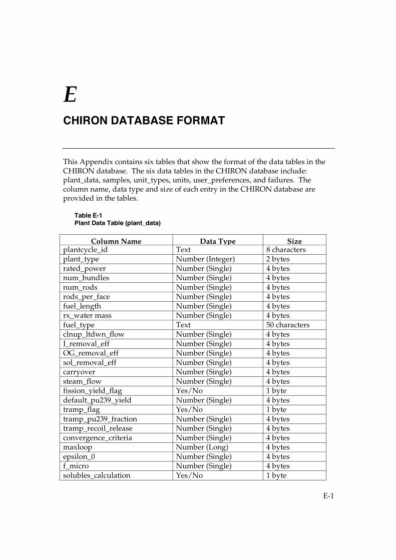
E-1
E CHIRON DATABASE FORMAT
This Appendix contains six tables that show the format of the data tables in theCHIRON database. The six data tables in the CHIRON database include:plant_data, samples, unit_types, units, user_preferences, and failures. Thecolumn name, data type and size of each entry in the CHIRON database areprovided in the tables.
Table E-1Plant Data Table (plant_data)
Column Name Data Type Sizeplantcycle_id Text 8 charactersplant_type Number (Integer) 2 bytesrated_power Number (Single) 4 bytesnum_bundles Number (Single) 4 bytesnum_rods Number (Single) 4 bytesrods_per_face Number (Single) 4 bytesfuel_length Number (Single) 4 bytesrx_water mass Number (Single) 4 bytesfuel_type Text 50 charactersclnup_ltdwn_flow Number (Single) 4 bytesI_removal_eff Number (Single) 4 bytesOG_removal_eff Number (Single) 4 bytessol_removal_eff Number (Single) 4 bytescarryover Number (Single) 4 bytessteam_flow Number (Single) 4 bytesfission_yield_flag Yes/No 1 bytedefault_pu239_yield Number (Single) 4 bytestramp_flag Yes/No 1 bytetramp_pu239_fraction Number (Single) 4 bytestramp_recoil_release Number (Single) 4 bytesconvergence_criteria Number (Single) 4 bytesmaxloop Number (Long) 4 bytesepsilon_0 Number (Single) 4 bytesf_micro Number (Single) 4 bytessolubles_calculation Yes/No 1 byte
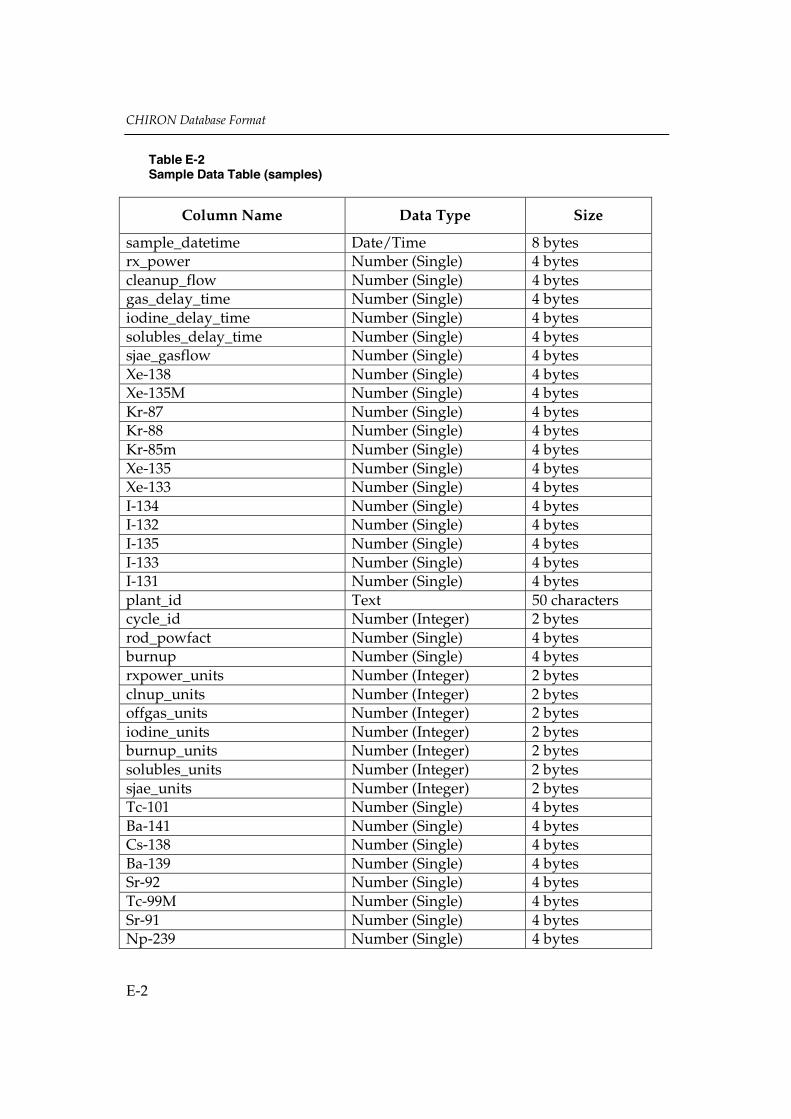
CHIRON Database Format
E-2
Table E-2Sample Data Table (samples)
Column Name Data Type Size
sample_datetime Date/Time 8 bytesrx_power Number (Single) 4 bytescleanup_flow Number (Single) 4 bytesgas_delay_time Number (Single) 4 bytesiodine_delay_time Number (Single) 4 bytessolubles_delay_time Number (Single) 4 bytessjae_gasflow Number (Single) 4 bytesXe-138 Number (Single) 4 bytesXe-135M Number (Single) 4 bytesKr-87 Number (Single) 4 bytesKr-88 Number (Single) 4 bytesKr-85m Number (Single) 4 bytesXe-135 Number (Single) 4 bytesXe-133 Number (Single) 4 bytesI-134 Number (Single) 4 bytesI-132 Number (Single) 4 bytesI-135 Number (Single) 4 bytesI-133 Number (Single) 4 bytesI-131 Number (Single) 4 bytesplant_id Text 50 characterscycle_id Number (Integer) 2 bytesrod_powfact Number (Single) 4 bytesburnup Number (Single) 4 bytesrxpower_units Number (Integer) 2 bytesclnup_units Number (Integer) 2 bytesoffgas_units Number (Integer) 2 bytesiodine_units Number (Integer) 2 bytesburnup_units Number (Integer) 2 bytessolubles_units Number (Integer) 2 bytessjae_units Number (Integer) 2 bytesTc-101 Number (Single) 4 bytesBa-141 Number (Single) 4 bytesCs-138 Number (Single) 4 bytesBa-139 Number (Single) 4 bytesSr-92 Number (Single) 4 bytesTc-99M Number (Single) 4 bytesSr-91 Number (Single) 4 bytesNp-239 Number (Single) 4 bytes

CHIRON Database Format
E-3
Column Name Data Type Size
Mo-99 Number (Single) 4 bytesTe-132 Number (Single) 4 bytesBa-140 Number (Single) 4 bytesTe-129M Number (Single) 4 bytesSr-89 Number (Single) 4 bytesCs-134 Number (Single) 4 bytesSr-90 Number (Single) 4 bytesCs-137 Number (Single) 4 bytesN-13 Number (Single) 4 bytesRb-89 Number (Single) 4 bytesNb-97 Number (Single) 4 bytesAr-41 Number (Single) 4 bytesCu-64 Number (Single) 4 bytesNa-24 Number (Single) 4 bytesZr-97 Number (Single) 4 bytesY-90 Number (Single) 4 bytesCr-51 Number (Single) 4 bytesFe-59 Number (Single) 4 bytesHf-181 Number (Single) 4 bytesZr-95 Number (Single) 4 bytesCo-58 Number (Single) 4 bytesZn-65 Number (Single) 4 bytesMn-54 Number (Single) 4 bytesCo-60 Number (Single) 4 bytes
Table E-3Unit Types Data Table (unit_types)
Column Name Data Type Size
unit_id Number (Integer) 2 bytesisa Number (Integer) 2 bytes

CHIRON Database Format
E-4
Table E-4Units Data Table (units)
Column Name Data Type Size
unit_id Number (Integer) 2 bytesunit_String Text 50 charactersunit_conversion Number (Integer) 2 bytesunit_NotReleaseRate Yes/No 1 byte
Table E-5User Preferences Data Table (user_preferences)
Column Name Data Type Size
user_id Number (Integer) 2 bytesoffgas_units Number (Integer) 2 bytesiodine_units Number (Integer) 2 bytesburnup_units Number (Integer) 2 bytescleanup_units Number (Integer) 2 bytespower_units Number (Integer) 2 bytessolubles_units Number (Integer) 2 bytessjae_units Number (Integer) 2 bytes

CHIRON Database Format
E-5
Table E-6Failures Data Table (failures)
Column Name Data Type Sizesample_datetime Date/Time 8 bytesplant_id Text 9 charactersis_record_valid Yes/No 1 byteOG_AEpsilon Number (Single) 4 bytesOG_Epsilon Number (Single) 4 bytesOG_C Number (Single) 4 bytesOG_FitError Number (Single) 4 bytesOG_ISConverged Yes/No 1 byteOG_Convergence Number (Single) 4 bytesOG_Iterations Number (Integer) 2 bytesOG_PuFraction Number (Single) 4 bytesOG_Failures Number (Single) 4 bytesI_AEpsilon Number (Single) 4 bytesI_Epsilon Number (Single) 4 bytesI_C Number (Single) 4 bytesI_FitError Number (Single) 4 bytesI_ISConverged Yes/No 1 byteI_Convergence Number (Single) 4 bytesI_Iterations Number (Integer) 2 bytesI_PuFraction Number (Single) 4 bytesI_Failures Number (Single) 4 bytesS_AEpsilon Number (Single) 4 bytesS_Epsilon Number (Single) 4 bytesS_C Number (Single) 4 bytesS_FitError Number (Single) 4 bytesS_ISConverged Yes/No 1 byteS_Convergence Number (Single) 4 bytesS_Iterations Number (Integer) 2 bytesS_PuFraction Number (Single) 4 bytesS_Failures Number (Single) 4 bytesCombinedFailures Number (Single) 4 bytesCalculatedRPF Number (Single) 4 bytesINPO_FRI Number (Single) 4 bytesCalculatedBU Number (Single) 4 bytesFuelReleaseDetected Yes/No 1 byteFuelReleaseRate Number (Single) 4 bytesXe138_Activity Number (Single) 4 bytesXe135m_Activity Number (Single) 4 bytesKr87_Activity Number (Single) 4 bytes

CHIRON Database Format
E-6
Column Name Data Type SizeKr88_Activity Number (Single) 4 bytesKr85m_Activity Number (Single) 4 bytesXe135_Activity Number (Single) 4 bytesXe133_Activity Number (Single) 4 bytesI134_Activity Number (Single) 4 bytesI132_Activity Number (Single) 4 bytesI135_Activity Number (Single) 4 bytesI133_Activity Number (Single) 4 bytesI131_Activity Number (Single) 4 bytesOG_Sum6 Number (Single) 4 bytesI_Sum5 Number (Single) 4 bytesXe138_Activity_N13 Number (Single) 4 bytesXe135m_Activity_N13 Number (Single) 4 bytesKr87_Activity_N13 Number (Single) 4 bytesKr88_Activity_N13 Number (Single) 4 bytesKr85m_Activity_N13 Number (Single) 4 bytesXe135_Activity_N13 Number (Single) 4 bytesXe133_Activity_N13 Number (Single) 4 bytesOG_Sum6_N13 Number (Single) 4 bytesTc101_Activity Number (Single) 4 bytesBa141_Activity Number (Single) 4 bytesCS138_Activity Number (Single) 4 bytesBa139_Activity Number (Single) 4 bytesSr92_Activity Number (Single) 4 bytesTc99_Activity Number (Single) 4 bytesSr91_Activity Number (Single) 4 bytesNp239_Activity Number (Single) 4 bytesMo99_Activity Number (Single) 4 bytesTe132_Activity Number (Single) 4 bytesBa140_Activity Number (Single) 4 bytesTe129m_Activity Number (Single) 4 bytesSr89_Activity Number (Single) 4 bytesCs134_Activity Number (Single) 4 bytesSr90_Activity Number (Single) 4 bytesCs137_Activity Number (Single) 4 bytesSol_Sum15 Number (Single) 4 bytesN13_Activity Number (Single) 4 bytesRb89_Activity Number (Single) 4 bytesNb97_Activity Number (Single) 4 bytesAr41_Activity Number (Single) 4 bytesCu64_Activity Number (Single) 4 bytes

CHIRON Database Format
E-7
Column Name Data Type SizeNa24_Activity Number (Single) 4 bytesZr97_Activity Number (Single) 4 bytesY90_Activity Number (Single) 4 bytesCr51_Activity Number (Single) 4 bytesFe59_Activity Number (Single) 4 bytesHf181_Activity Number (Single) 4 bytesZr95_Activity Number (Single) 4 bytesCo58_Activity Number (Single) 4 bytesZn65_Activity Number (Single) 4 bytesMn54_Activity Number (Single) 4 bytesCo60_Activity Number (Single) 4 bytesXe138_PredAct Number (Single) 4 bytesXe135m_PredAct Number (Single) 4 bytesKr87_PredAct Number (Single) 4 bytesKr88_PredAct Number (Single) 4 bytesKr85m_PredAct Number (Single) 4 bytesXe135_PredAct Number (Single) 4 bytesXe133_PredAct Number (Single) 4 bytesOG_Sum6_fitted Number (Single) 4 bytesOG_Sum6_tramp_fitted Number (Single) 4 bytesXe138_PredAct_FRC Number (Single) 4 bytesXe135m_PredAct_FRC Number (Single) 4 bytesKr87_PredAct_FRC Number (Single) 4 bytesKr88_PredAct_FRC Number (Single) 4 bytesKr85m_PredAct_FRC Number (Single) 4 bytesXe135_PredAct_FRC Number (Single) 4 bytesXe133_PredAct_FRC Number (Single) 4 bytesOG_Failures_FRC Number (Single) 4 bytesOG_Epsilon_FRC Number (Single) 4 bytesOG_AEpsilon_FRC Number (Single) 4 bytesOG_C_FRC Number (Single) 4 bytesOG_FitError_FRC Number (Single) 4 bytesOG_PuFraction_FRC Number (Single) 4 bytesOG_Sum6_fitted_FRC Number (Single) 4 bytesOG_Sum6_tramp_fitted_FRC Number (Single) 4 bytesOG_CalculatedBU_FRC Number (Single) 4 bytesI134_PredAct Number (Single) 4 bytesI132_PredAct Number (Single) 4 bytesI135_PredAct Number (Single) 4 bytesI133_PredAct Number (Single) 4 bytesI131_PredAct Number (Single) 4 bytes

CHIRON Database Format
E-8
Column Name Data Type SizeI_Sum5_fitted Number (Single) 4 bytesI_Sum5_tramp_fitted Number (Single) 4 bytesI134_PredAct Number (Single) 4 bytesI132_PredAct Number (Single) 4 bytesI135_PredAct Number (Single) 4 bytesI133_PredAct Number (Single) 4 bytesI131_PredAct Number (Single) 4 bytesI_Failures_FRC Number (Single) 4 bytesI_Epsilon_FRC Number (Single) 4 bytesI_AEpsilon_FRC Number (Single) 4 bytesI_C_FRC Number (Single) 4 bytesI_FitError_FRC Number (Single) 4 bytesI_PuFraction_FRC Number (Single) 4 bytesI_Sum5_fitted_FRC Number (Single) 4 bytesI_Sum5_tramp_fitted_FRC Number (Single) 4 bytesI_CalculatedBU_FRC Number (Single) 4 bytesTc101_PredAct Number (Single) 4 bytesBa141_PredAct Number (Single) 4 bytesCs138_PredAct Number (Single) 4 bytesBa139_PredAct Number (Single) 4 bytesSr92_PredAct Number (Single) 4 bytesTc99m_PredAct Number (Single) 4 bytesSr91_PredAct Number (Single) 4 bytesNp239_PredAct Number (Single) 4 bytesMo99_PredAct Number (Single) 4 bytesTe132_PredAct Number (Single) 4 bytesBa140_PredAct Number (Single) 4 bytesTe129m_PredAct Number (Single) 4 bytesSr89_PredAct Number (Single) 4 bytesCs134_PredAct Number (Single) 4 bytesSr90_PredAct Number (Single) 4 bytesCs137_PredAct Number (Single) 4 bytesSol_Sum15_fitted Number (Single) 4 bytesSol_Sum15_tramp_fitted Number (Single) 4 bytesDelta_Zr95 Number (Single) 4 bytesDamage_Zr95 Number (Single) 4 bytesINPO_FRI_SampleValue Number (Single) 4 bytesBU_CsRatio Number (Single) 4 bytesPower_Fraction Number (Single) 4 bytesSample_RPF Number (Single) 4 bytesSample_BU Number (Single) 4 bytes

i
INDEX
A
a Coefficient .......................... 6-9, 6-10
Active Fuel Length ............... 3-5, 6-18
Activity ..........................................6-23
Iodine.........................................3-13
Offgas.........................................3-13
Negative ..................................... 4-3
Solubles......................................3-13
Analysis Summary screen............. 4-1
Analyze Batch ......................2-19, 2-21
Analyze Single ..............................2-19
ASCII Dump File ................2-15, 2-21,4-19, 5-4 , D-1 - D-9
a Coefficient......4-13, 6-12, 6-14, 6-15
B
Batch
Analyze.............................2-19, 2-21
Input Files..................................3-15
Time-Select ................................2-23
Bitmap File ....................................2-27
Booth Formulation......................... 6-6
Burnup.........................3-12, 4-18, 6-16
BWR Failure Correlation............... 4-8
C
C Coefficient........ 4-7, 4-13, 6-9, 6-10,6-12, 6-14, 6-15
C( ) vs. Plot......... See Plot, C( ) vs.
Calculation Log.............................4-19
Calculation Log File .....................2-15
Cardinal Units................................ 3-1
chicalc.log.............................2-15, 4-19
CHIRON
Installation.................................. 2-2
Setup ........................................... 2-1
CHIRON DB ........................... 2-7, 3-3

Index
ii
Cleanup/Letdown
Flow Density ... 3-6, 6-21, 6-23, 6-24
Flow Rate.................. 3-12, 6-1, 6-21
Convergence Error .......................4-13
Convergence Limit ........................ 3-8
Cs-Ratio .........................................4-18
D
Data Entry
File Format ........................ 3-14, B-1
File Input ........................... 3-1, 3-14
Range Checking ....... 3-5, 3-12, 3-14
Screen Input ...................... 3-1, 3-10
Data Source .................................... 2-8
Database
Blank ..........................................2-12
Compacting ................................ 5-3
Conversion ........................ 2-11, 5-4
Creation ...................................... 5-2
Distribution ................................ 2-1
Filename .............................. 2-8, 3-4
Overview .................................... 5-1
Registration ......................... 2-6, 2-8
Sample .......................................2-12
Selection.....................................2-13
Database Table
failures ........................ 5-2, E-5 - E-8
plant_data............................5-1, E-1
samples ................................5-1, E-2
unit_types............................5-2, E-3
units .....................................5-2, E-4
user_preferences .................5-2, E-4
DBConvert...................................... 5-4
Decay Constant..................... 6-2, 6-11
Default Pu239 Fraction..................... 3-7
Diffusion Rate ................................ 6-4
E
Efficiency
Iodine Removal................. 3-6, 6-22
Offgas Removal................. 3-6, 6-22
Rx Solubles Removal ........ 3-6, 6-22
Empirical Coefficients ..................6-17
Coefficient 4-6, 4-7, 4-13, 6-9, 6-10,6-12, 6-13, 6-15
Epsilon_0 ........................................ 3-8
Index
iii
Equilibrium Equations .................. 6-1
Error Message
Data Input .................................. 7-1
Database ..................................... 7-4
Miscellaneous............................. 7-7
Escape Rate Coefficient................. 6-6
Example Files ................................ A-4
F
F( ) vs. Plot .......... See Plot, F( ) vs.
Failure Correlation Plot.................................. See Plot, Failure Correlation
Failure Model.....6-11, 6-15, 6-19, 6-34
Combined .........................6-26, 6-34
Fission Rate .................................... 6-3
Fission Yields ................................. 6-2
Fit Summary Report .....................2-20
Fuel Microstructure.............. 3-8, 6-31
Fuel Rods per Assembly Face....... 3-5
G
Gas Delay Time.............................3-12
Grid lines.......................................2-25
I
INPO FRI.......................................6-38
Installation...................................... 2-2
Compact...................................... 2-4
Custom........................................ 2-5
Location ...................................... 2-3
Type ............................................ 2-3
Typical ........................................ 2-4
Iodine
Activity ............See Activity, Iodine
Delay Time ................................3-13
Removal Efficiency .............................See Efficiency, Iodine Removal
L
Least Squares Analysis.................6-10
Letdown ........ See Cleanup/Letdown
Linear Heat Generation Rate ......6-17, 6-29
Loop on Fission Yield.................... 3-7

Index
iv
M
Main Program Window ...............2-12
Maximum Loops............................ 3-8
Metafile..........................................2-27
Microsoft Access ............................ 5-1
Microsoft Access Driver................ 2-6
Microsoft Excel .............................3-15
N
Number of Assemblies.................. 3-5
Number of Fuel Rods ........... 3-5, 6-18
O
ODBC.............................................. 5-3
Administrator ............................ 2-6
Drivers ................................. 2-5, 5-1
Files ............................................ A-1
Offgas
Activity ............See Activity, Offgas
Delay Time ................................3-12
Removal Efficiency ............................ See Efficiency, Offgas Removal
OLE Drivers ................................... 2-5
OLE Files ....................................... A-3
ORIGEN Curves ............................ 4-5
Outage Schedule............................ 4-5
Output Options.............................2-15
P
Plant Cycle
Select ..........................................2-16
Plant Cycle History ....................... 4-5
Plant-Cycle Configuration ... 2-16, 3-2
Plant-Cycle ID....... 2-16, 3-2, 3-12, 5-5
Plot
C( ) vs. .....................................
Cs Ratio vs. Burnup................... 4-5
Customization...........................2-24
Export ........................................2-27
F( ) vs. ......................................
Failure Correlation .................... 4-8
Grid Lines..................................2-26
Help ...........................................2-27
Numeric Precision ....................2-25
Options ......................................2-25

Index
v
R/B vs. Lambda.................. 4-2, 4-3
Selection...................2-19, 2-22, 2-24
Trend.................................. 2-22, 4-9
Trend Options ............................ 4-9
Zoom..........................................2-29
Printing..........................................2-30
Program DLL Files ........................ 3-3
Program Files ................................. 3-4
Pu Fission Fraction .............. 6-8 - 6-10
R
R2-Value................................4-13, 6-10
Reactor Power...............................3-12
Reactor Rated Power ..... 3-4, 3-5, 6-18
Reactor Water Volume.........3-5, 6-21,6-23, 6-24
Readme File...................................2-11
References ...................................... 8-1
Release Rate Conversion..............6-20
Release to Birth .............................6-11
Iodine.........................................4-16
Offgas.........................................4-15
Solubles......................................4-17
Report
Activity Ratio ............................4-18
Calculation Log.........................4-19
Fit Summary..............................2-20
Iodine Activity Summary.........4-14
Iodine Release to Birth Summary................................................4-16
Offgas Activity Summary ........4-13
Offgas Release to Birth Summary................................................4-15
QA......................................4-19, C-1
Selection.....................................2-19
Solubles Activity Summary .....4-15
Solubles Release to Birth Summary................................................4-17
Rod Power Factor ...............3-12, 6-17, 6-18, 6-26
Rx Solubles Activity ...................................................See Activity, Solubles
Rx Solubles Removal Efficiency .........See Efficiency, Rx SolublesRemoval
S
Sample Date ..................................3-12
Sample Time .................................3-12
Index
vi
Samples
Select ..........................................2-17
Screen Reports ..............................4-12
Setup ....................See CHIRON:Setup
SJAE Flow Rate ............ 3-13, 5-5, 6-23
Small Defects.................................6-14
Soluble Delay Time ......................3-13
Solubles Calculation............. 2-16, 3-7
Steam Carryover................... 6-1, 6-25
Steam Flow....................................6-25
System Requirements.................... 2-1
T
Three-Coefficient Fit............. 4-7, 6-10
Time-Select Batch..........................2-23
Toggle Status........................2-18, 2-24
Tramp ............................................. 4-2
Diffusion..................................... 6-7
Diffusion Coefficient ................. 6-9
Fission Rate ................................ 6-4
Recoil Fraction ........................... 3-7
Yield Calculation ....................... 3-7
Yield Fraction............. 3-7, 6-4, 6-10
Trend Plots .................. See Plot:Trend
Tutorial ..........................................2-12
Two-Coefficient Fit............... 4-7, 6-14
U
Uninstall ........................................2-11
Units
Cardinal ...................................... 3-1
Conversion .......................... 3-1, 3-2
Edit..................................... 3-1, 3-10
Z
Zoom...................................... 2-29, 4-6
EPRI • 3412 Hillview Avenue, Palo Alto, California 94304 • PO Box 10412, Palo Alto, California 94303 • USA800.313.3774 • 650.855.2121 • [email protected] • www.epri.com
WARNING: This Document containsinformation classified under U.S. ExportControl regulations as restricted fromexport outside the United States. You
are under an obligation to ensure that you have alegal right to obtain access to this informationand to ensure that you obtain an export licenseprior to any re-export of this information. Specialrestrictions apply to access by anyone that is nota United States citizen or a Permanent UnitedStates resident. For further informationregarding your obligations, please see theinformation contained below in the section titled“Export Control Restrictions.”
© 1998 Electric Power Research Institute (EPRI), Inc.All rights reserved. Electric Power ResearchInstitute and EPRI are registered service marks of the Electric Power Research Institute, Inc.EPRI. ELECTRIFY THE WORLD is a service mark of the Electric Power Research Institute, Inc.
Printed on recycled paper in the United States of America
: 1011048
About EPRI
EPRI creates science and technology solutions forthe global energy and energy services industry.U.S. electric utilities established the Electric PowerResearch Institute in 1973 as a nonprofit researchconsortium for the benefit of utility members, theircustomers, and society. Now known simply as EPRI,the company provides a wide range of innovativeproducts and services to more than 1000 energy-related organizations in 40 countries. EPRI’smultidisciplinary team of scientists and engineersdraws on a worldwide network of technical andbusiness expertise to help solve today’s toughestenergy and environmental problems.
EPRI. Electrify the World
Export Control RestrictionsAccess to and use of EPRI Intellectual Property is grantedwith the specific understanding and requirement thatresponsibility for ensuring full compliance with all applicableU.S. and foreign export laws and regulations is beingundertaken by you and your company. This includes anobligation to ensure that any individual receiving accesshereunder who is not a U.S. citizen or permanent U.S.resident is permitted access under applicable U.S. and foreignexport laws and regulations. In the event you are uncertain whether you oryour company may lawfully obtain access to this EPRIIntellectual Property, you acknowledge that it is your obligation to consult with your company’s legal counsel todetermine whether this access is lawful. Although EPRI maymake available on a case by case basis an informal assessmentof the applicable U.S. export classification for specific EPRIIntellectual Property, you and your company acknowledgethat this assessment is solely for informational purposes andnot for reliance purposes. You and your company acknowledge that it is still the obligation of you and yourcompany to make your own assessment of the applicableU.S. export classification and ensure compliance accordingly.You and your company understand and acknowledge yourobligations to make a prompt report to EPRI and the appropriate authorities regarding any access to or use ofEPRI Intellectual Property hereunder that may be in violationof applicable U.S. or foreign export laws or regulations.