K. Baysal, T. Schafhitzel, T. Ertl, U. Rist: Extraction and Visualization of Flow Features

in: W. Nitsche, C. Dobriloff (Eds.): Imaging Measurement Methods for Flow Analysis, results of theDFG priority programme 1147 Imaging Measurement Methods for Flow Analysis 2003-2009

NNFM 106, Springer, 2009, 305–314.

Extraction and Visualization of Flow Features

Kudret Baysal and Tobias Schafhitzel and Thomas Ertl and Ulrich Rist

Abstract This paper presents tools which allow an advanced investigation of spatialand temporal progress of segmented vortex structures in flow fields with the consid-eration of vortex dynamics. The work is based on the local and Eulerian detectionand segmentation of vortex structures and the visualization of these structures withrecent visualization methods, e.g. the application of LIC-textures on the surfacesof 3d structures. The second step is the tracking of vortex structures based on thetime-dependent integration of vortex core lines. In the third step, according to thevortex dynamics, the individual degree of impact is determined by computation ofinduced velocities via the Biot-Savart equation for each vortex. The induced veloc-ities are used to determine the induced kinetic energy and enstrophy, which allowsthe evaluation of a global value of influence for each vortex structure, that can betracked in time.

1 Introduction

The physical understanding of boundary layers or mixing layers is of fundamentalinterest for fluid dynamical research. A principal method in the investigations ofphysical aspects of flow fields is the observation of characteristic features of theflow fields, which are coherent in space and time. Although the so-called coherentstructures or vortex structures are well-known in the analysis of flow fields, e.g.laminar-turbulent transition or effects of flow control mechanisms, the investigationsof real-life flow fields based on coherent structures are not straightforward.

The aim of this paper is to present techniques for an advanced investigation ofthree-dimensional and time-dependent flow fields. The first goal of this work is the

Kudret Baysal and Ulrich RistInstitut fur Aerodynamik und Gasdynamik, Universitat Stuttgart, Pfaffenwaldring 21, 70569Stuttgart, Germany, e-mail: baysal—rist@iag.uni-stuttgart.de

Tobias Schafhitzel and Thomas ErtlInstitut fur Visualisierung und Interaktive Systeme, Universitat Stuttgart, Universitatsstrasse 38,70569 Stuttgart, e-mail: schafhitzel—ertl@vis.uni-stuttgart.de

1

2 Kudret Baysal and Tobias Schafhitzel and Thomas Ertl and Ulrich Rist

automatic identification and segmentation of vortex structures in order to find anappropriate visualization, which allows the engineer to investigate the extracted fea-tures in an interactive manner. For the visualization, recent algorithms have been ap-plied, which exploit newest graphics hardware features. This is followed by vortextracking, i.e., the time-dependent mapping of individual vortex structures to capturetheir temporal development. For this purpose, a framework has been developed,which provides, beside the investigation of vortices in a single snapshot, also thetime-dependent visualization of these structures. This allows an advanced analy-sis of kinematic properties of the vortex structures, e.g. size, shape, and vorticitystrength. The results of these studies allow the acquisition of quantitative informa-tion for flow fields, which are necessary in the development of flow field models orin the comparison and validation of experimental and numerical studies.

The second goal is the consideration of vortex dynamical effects, which allowsthe study of interactions between vortex structures, e.g. vortex merging, and self-excited effects, e.g. the autogeneration of hairpin vortices, which is a significantmechanism in the generation of turbulence. The strategy of this work is the determi-nation of the velocity field induced by each vortex structure in a flow field and theirinfluence in the time-dependent development of other vortex structures. In order tosupport the consideration of vortex dynamics within our framework, the engineer isable to select an arbitrary vortex structure, which is then used to determine the timeas well as the vortex structure which perturbs the selected vortex strongest. Thetime-dependent dynamical investigation of interactions between structures enablesthe investigation of effectiveness of flow-control mechanisms.

2 Flow-Features Identification

The main vortex identification methods are based on the widely accepted defini-tion of a vortex structure as a finite volume of fluid particles with a vortical mo-tion around a center line. The complexity of the vortex structures and lacks in theunderstanding of these structures caused discussions of different aspects of vortexstructures and their identification. This resulted in several approaches for vortexidentification, whereby the focus was for the last few years on the influence of axialstretching and shearing [3] on vortex identification, as investigations of vortex re-gions with high shear had revealed a gap in the reliability of the widely used criteria,e.g. λ2 [2] or the Okubo-Weiss criterion, also known as Q criterion.

Although the influence of high-shear regions in the identification of vortex struc-ture regions is in the focus of discussions, the understanding of it is still not clear.Hence it is necessary to analyze the effects of shearing on vortex structure identifi-cation and vortex dynamics.

One of the latest approaches, which is considering the effects of shear in the vor-tex identification, is the approach of Kolar [3]. The triple decomposition method ofKolar is an extension of the classical decomposition of the velocity gradient tensor∇u into a symmetric and an asymmetric part. The motivation of the new decompo-sition is the fact that the asymmetric tensor, which holds the vorticity, is not able todistinguish between pure shearing motion and vortical motion. Therefore, the de-

Extraction and Visualization of Flow Features 3

composition of ∇u into three tensors is desirable, where the third tensor describespure shear motion and the new corrected vorticity tensor considers only vortical mo-tion. Although the application of the new criterion for two-dimensional examples,e.g. mixing layers, is promising, the lack of an algorithm for three-dimensional flowfields makes a general application impossible, at present.

For the examples in the following sections the λ2 criterion is used, which is,despite its inaccuracies in high-shear regions, the most reliable criterion for three-dimensional flow fields.

3 Visualization of Vortices

The goal of our project was to provide an interactive visual representation of vortexstructures. Therefore, the following subgoals should be accomplished: (1) vortexsegmentation. This step is crucial for separating arbitrarily connected vortex struc-tures, like those resulting from conventional isosurface- generation algorithms; (2)vortex visualization. Based on the foregoing segmentation step, the vortices needto be visualized appropriately; (3) multi-field visualization, i.e., the visualization ofvortices and additional quantities, e.g., the velocity field; (4) vortex tracking. Sincemost of the underlying velocity fields represent a time-dependent flow, an appropri-ate time-dependent visualization of vortex structures is needed.

3.1 Vortex Segmentation

The role of vortex segmentation can be illustrated by a simple scenario. Imagine wehave a scalar field like the one that results from the λ2 computation. Then, from thepoint of view of visualization there are various methods for drawing an isosurfaceof this input data, which represents, according to the theory of λ2, the vortex bound-aries if the isovalue is set to a small value below zero in order to avoid artifacts dueto noisy data.

Our goal was to provide the engineer more interactivity in terms of selectingsingle vortex structures, fading them out, or simply to investigate them in moredetail. Therefore, a criterion, which delivers a list of segmented vortices must befound–the vortex core line. We define a vortex core line as a connected set of localpressure (or λ2) minima. The end points of a vortex core line are found by searchingfor discontinuities of the core line tangent or by checking if the function value ofthe core line becomes positive. A predictor-corrector method by Stegmaier et al. [8]is used for computing the vortex core lines: first a list of seed points is generated.Since 3D minima of λ2 are a subclass of the local λ2 minima discussed above, theymust be part of the vortex core line and, therefore, can serve as seed points withoutany restrictions.

Once the list of seed points has been generated, the algorithm starts by process-ing them in a consecutive order. Each seed point is tested if it is inside the vortexboundaries, the λ2 = 0 isosurface, of an already detected vortex. If this is the case,the seed point is discarded. Otherwise it serves as first point p0 on the growing vor-

4 Kudret Baysal and Tobias Schafhitzel and Thomas Ertl and Ulrich Rist

(a) (b)

Fig. 1 Visualization of a segmented vortex field: Figure (a) shows the λ2 isosurfaces colored ac-cording to the vortex strength. Here, the gradient goes from green (= weak) to red (= strong);Figure (b) demonstrates the interactivity of our framework. Individual vortices can be selected andtransformed while uninteresting vortices are blended out and drawn as small quadrilaterals at thetop of the screen.

tex core line, where both a prediction and a correction step are performed. Sincethe vorticity can be regarded as the local axis of rotation and we assume that thevortex rotates around the vortex core line, it can be used for predicting the nextposition on the core line. However, an integration along the vorticity vector wouldinvolve a numerical error, which need to be corrected in a second step. Here, againthe vorticity is computed, now at the predicted position. The corrected position pi+1is finally found by searching for the λ2 minimum on a plane perpendicular to thevorticity. Then the loop is repeated, using pi+1 as starting point until a discontinuityof the core line is detected or λ2 becomes positive. In order to identify all vortex corelines, the algorithm is performed over all seed points. For a more detailed discussionwe refer to [8].

In a last step, the isosurfaces are computed for each vortex individually by creat-ing planes at the computed positions pi. The geometrical data is stored together withthe points and the topology of the vortex core lines into appropriate data structures,which are discussed in Section 3.2.

3.2 Vortex Visualization

Once the vortices and their respective core lines are computed, they to need be storedinto data structures which are appropriate for an interactive visualization. Here, thegoal of vortex visualization exceeds a simple visualization of their λ2 isosurfaces—apart from a good visual representation, the user should be able to interact with thevisualized data. Therefore, the following features should be supported: (1) globaltransformation of all vortices; (2) selection and transformation of individual vortexstructures; and (3) removal of uninteresting vortices.

Extraction and Visualization of Flow Features 5

(a) (b) (c)

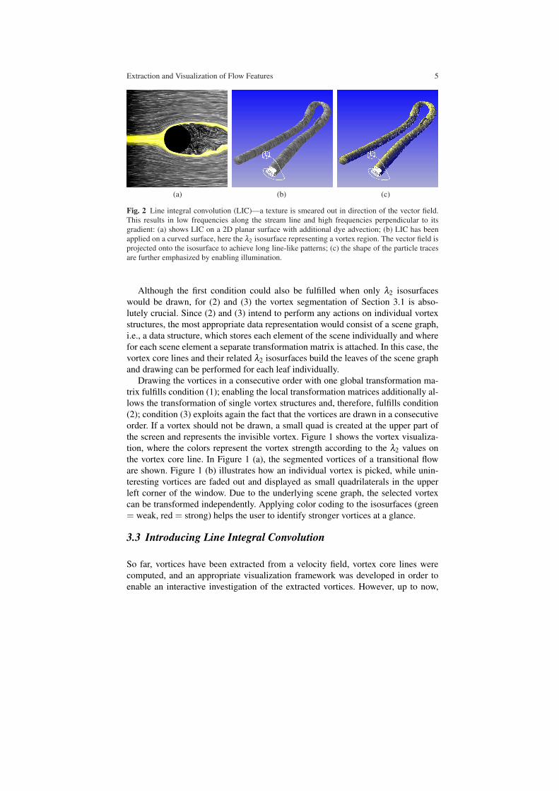
Fig. 2 Line integral convolution (LIC)—a texture is smeared out in direction of the vector field.This results in low frequencies along the stream line and high frequencies perpendicular to itsgradient: (a) shows LIC on a 2D planar surface with additional dye advection; (b) LIC has beenapplied on a curved surface, here the λ2 isosurface representing a vortex region. The vector field isprojected onto the isosurface to achieve long line-like patterns; (c) the shape of the particle tracesare further emphasized by enabling illumination.

Although the first condition could also be fulfilled when only λ2 isosurfaceswould be drawn, for (2) and (3) the vortex segmentation of Section 3.1 is abso-lutely crucial. Since (2) and (3) intend to perform any actions on individual vortexstructures, the most appropriate data representation would consist of a scene graph,i.e., a data structure, which stores each element of the scene individually and wherefor each scene element a separate transformation matrix is attached. In this case, thevortex core lines and their related λ2 isosurfaces build the leaves of the scene graphand drawing can be performed for each leaf individually.

Drawing the vortices in a consecutive order with one global transformation ma-trix fulfills condition (1); enabling the local transformation matrices additionally al-lows the transformation of single vortex structures and, therefore, fulfills condition(2); condition (3) exploits again the fact that the vortices are drawn in a consecutiveorder. If a vortex should not be drawn, a small quad is created at the upper part ofthe screen and represents the invisible vortex. Figure 1 shows the vortex visualiza-tion, where the colors represent the vortex strength according to the λ2 values onthe vortex core line. In Figure 1 (a), the segmented vortices of a transitional floware shown. Figure 1 (b) illustrates how an individual vortex is picked, while unin-teresting vortices are faded out and displayed as small quadrilaterals in the upperleft corner of the window. Due to the underlying scene graph, the selected vortexcan be transformed independently. Applying color coding to the isosurfaces (green= weak, red = strong) helps the user to identify stronger vortices at a glance.

3.3 Introducing Line Integral Convolution

So far, vortices have been extracted from a velocity field, vortex core lines werecomputed, and an appropriate visualization framework was developed in order toenable an interactive investigation of the extracted vortices. However, up to now,

6 Kudret Baysal and Tobias Schafhitzel and Thomas Ertl and Ulrich Rist

only the locations, the spatial extents, and the vortex strengths are perceptible forthe user—there is no possibility to identify the direction of rotation of the individualvortices so far! This information, though, is quite important because it plays a crucialrole in vortex dynamics, where the direction of rotation of a vortex is of specialmeaning considering the amplification of other vortices (see Section 5).

For this purpose, the flow feature visualization described above is combined witha real-time texture-based flow visualization technique–the line integral convolution(LIC) algorithm [1]–which is a common method in computer graphics. The majoradvantage of this algorithm is that it exploits the capabilities of modern graphicshardware and, therefore, is highly interactive. Without going into technical detail,LIC is actually used to draw stream lines by integrating along a given vector field,whereby stream lines appear as lines of low frequencies. A result of 2D LIC isshown in Figure 2 (a). Since the original LIC algorithm is not appropriate for draw-ing stream lines on curved surfaces as those which result from our vortex visual-ization algorithm of section 3.2, an extended version by Weiskopf and Ertl [9] hasbeen applied to the λ2 isosurfaces. Based on the fact that the velocity field is almosttangential to the λ2 = 0 isosurface, the vector field is projected onto the isosurface.This results in line-like patterns on the λ2 isosurfaces and has the following advan-tages: (1) the motion of a particle close to a vortex region is perceptible at a glance;and (2) applying animated LIC, the direction of rotation is perceptible as well with-out loosing the information provided by the vortex visualization. Figure 2 (b) and(c) show LIC on vortex surfaces, whereby in (c) the particle traces are further em-phasized by illumination. For a more detailed discussion we refer to the work ofSchafhitzel et al. [5].

4 Vortex Tracking

Considering unsteady vector fields instead of individual snapshots, the temporalbehavior of the extracted vortex structures are of special interest because this infor-mation can be used for detecting temporal events. The mapping of vortex structures,which have been extracted at time t to their counterparts at a later time step t +∆ t iscalled vortex tracking and builds the base of any temporal investigation of vortices.

The tracking algorithm we used is based on the work of Schafhitzel et al. [6],where the vortex core line at time t is sampled and particles are integrated alongthe vector field in order to estimate the new position of the vortex core line at timet + ∆ t. This method is simple and reliable, since the vortex core line is supposedto be the region inside a vortex which exceeds at least the upper boundary of λ2(λ2 = 0) and, therefore, the particles seeded on the vortex core lines do not tend toleave the vortex from t to t +∆ t.

Our framework, which is represented in Figure 3, supports user interactivity inthe following manner: (1) the user is able to select a single vortex at an arbitrary timestep in order to track it forward and backward along the time-dependent vector field.Here, all the relationships between the vortices at the different time steps are created;(2) a time line is provided, which can be used to manipulate the time at whichthe vortex should be visualized. By smoothly sliding the red bar along the time

Extraction and Visualization of Flow Features 7

(a) (b)

(c) (d)

Fig. 3 The visualization of an experimental data set [4]. The data was measured using tomographicPIV and shows a circular cylinder wake at Reynolds Re = 360. The cylinder, which is locatedparallel to the left edge of the data set is not visualized. In this example, vortex dynamics areconsidered: (a) initial situation at t = 0. All vortices are color coded according to their strength.The red bounding box gives feedback about the vortex selected for tracking; (b) the moment ofstrongest perturbation at tp = 4. The representation has changed to time tp where the green vortexinfluences the selected structure (red); (c) backward tracking. The wire frame representation showswhere the structures came from; (d) forward tracking. Here, the wire frame representation showsthe further development of both structures [6]. c©2008 by Schafhitzel et al.

line, the transitions between the time steps are visualized; (3) topological changesare supported when a vortex core line hits more than one structure. Note that thedetection of vortex reconnection events depends on the quality of the underlyingvortex core line detection method. For a topology-preserving λ2-based vortex coreline detection method we refer to the work of Schafhitzel et al. [7]. Altogether,this method provides a fast and interactive investigation of vortices inside a time-dependent flow because once a vortex has been selected and tracked, the user is ableto switch between the different time steps very fast.

8 Kudret Baysal and Tobias Schafhitzel and Thomas Ertl and Ulrich Rist

5 Considering Vortex Dynamics

The analysis of coherent structures is based on the purpose to gain physical un-derstanding of the mechanisms in fluid dynamics, which is necessary for a reli-able comparability of experimental and numerical studies, the reproducibility ofthese studies, or predictive modeling of flow field regions, e.g. separated flows andwakes. A method for the detection of vortex core lines is described in Section 3.1;the tracking of vortices is discussed in Section 4. These methods enable the spatialand temporal investigation of kinematic properties (e.g. size, vorticity, and energy)of vortex structures and, therefore, provide quantitative information for an advancedcomparison of studies and physical models.

However, an analysis of coherent structures, which is limited to kinematic proper-ties cannot be sufficient in the investigation of central questions in the developmentof flow fields. Hence, an additional investigation of the dynamic properties (e.g.emergence, growth, and stability) of the coherent structures is necessary to answerthese questions.

A straightforward strategy for the consideration of vortex dynamics in the analy-sis of coherent structures is the observation of dynamical values, e.g., kinetic energyor enstrophy, which are defined by

Ekin =12

∫

V(u(x, t))2 d3x and Erot =

12

∫

Vω (x, t)2 d3x , (1)

respectively, where ω denotes vorticity. Thereby, several problems arise: the first isthe lack of a proper definition of the region of integration. In test cases with twovortex structures like collision of vortex rings, it is sufficient to integrate over thewhole domain. However, in real flow fields containing hundreds of structures ofinterest, each of them needs a more specified definition of the integrated volume. Areasonable choice are the spatial extents of the vortical regions.

The second problem addresses a major aspect in the investigation of dynamicalproperties–the interaction between coherent structures–like the merging of coherentstructures or the self-excited effects of complex coherent structures (e.g. hairpinvortices). A technique which deals with these effects is the determination of theinduced velocities of each coherent structure. The fundamental equation for thistechnique is the Biot-Savart equation, which computes the induced velocity fieldout of the vorticity field:

uind(x, t) =1

4π

∫

V

ω(x′, t)× (x−x′)|x−x′|3 d3x′ , (2)

where the influence of x′ on x is computed.A pure monitoring of the induced velocities has only a limited significance for a

characterization of the interaction between coherent structures because the consid-eration of the influences on a vector field is not straightforward. Hence, an approach,which combines both methods described above is used to determine the interactionof coherent structures. For this purpose, the influence of one vortex structure on an-

Extraction and Visualization of Flow Features 9

Store

Core Line and

λ2 Surface

Preprocessing Real Time Processing

Compute

Vortex Core

Lines

for each vortex

Track

Vortex

Structure

Compute

kinetic energy

and enstrophy

Evaluate

Biot-Savart

Equation

for each selected structure and for each time step

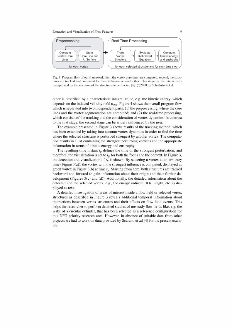
Fig. 4 Program flow of our framework: first, the vortex core lines are computed; second, the struc-tures are tracked and computed for their influence on each other. This stage can be interactivelymanipulated by the selection of the structures to be tracked [6]. c©2008 by Schafhitzel et al.

other is described by a characteristic integral value, e.g. the kinetic energy, whichdepends on the induced velocity field uind . Figure 4 shows the overall program flowwhich is separated into two independent parts: (1) the preprocessing, where the corelines and the vortex segmentation are computed; and (2) the real-time processing,which consists of the tracking and the consideration of vortex dynamics. In contrastto the first stage, the second stage can be widely influenced by the user.

The example presented in Figure 3 shows results of the tracking method, whichhas been extended by taking into account vortex dynamics in order to find the timewhere the selected structure is perturbed strongest by another vortex. The computa-tion results in a list containing the strongest perturbing vortices and the appropriateinformation in terms of kinetic energy and enstrophy.

The resulting time instant tp defines the time of the strongest perturbation, andtherefore, the visualization is set to tp for both the focus and the context. In Figure 3,the detection and visualization of tp is shown. By selecting a vortex at an arbitrarytime (Figure 3(a)), the vortex with the strongest influence is computed, displayed asgreen vortex in Figure 3(b) at time tp. Starting from here, both structures are trackedbackward and forward to gain information about their origin and their further de-velopment (Figures 3(c) and (d)). Additionally, the detailed information about thedetected and the selected vortex, e.g., the energy induced, IDs, length, etc. is dis-played as text.

A detailed investigation of areas of interest inside a flow field or selected vortexstructures as described in Figure 3 reveals additional temporal information aboutinteractions between vortex structures and their effects on flow-field events. Thishelps the researcher to perform detailed studies of unsteady flow fields like, e.g. thewake of a circular cylinder, that has been selected as a reference configuration forthis DFG priority research area. However, in absence of suitable data from otherprojects we had to work on data provided by Scarano et .al [4] for the present exam-ple.

10 Kudret Baysal and Tobias Schafhitzel and Thomas Ertl and Ulrich Rist

6 Conclusions

Recent flow-field measurements techniques such as those considered within thepresent DFG priority research program are capable of producing several gigabytesof raw data within a short time. Without appropriate post-processing and visualiza-tion methods the physical insight hidden in these data would remain unexplored.The methods presented here allow the researcher an interactive exploration of suchdata on a higher abstraction level based on the concept of “vortices”. As such, vor-tex identification, segmentation, quantification and tracking are a prerequisite forany detailed investigation of unsteady separated flows, which might be encounteredafter boundary layer separation, in mixing layers or in wakes. However, the presenttool is not yet complete,. It still lacks more methods for an automatic tracking ofevents like vortex creation out of shear or vortex merging. According work is nec-essary and in progress.

7 Acknowledgments

We thank the DFG for financial support of this work under grants ER 272/4 andRI 680/14 and we are very grateful to Fulvio Scarano, TU Delft for providing thecylinder data set used in the present article.

References

1. Cabral B, Leedom L C (1993) Imaging Vector Fields Using Line Integral Convolution. Proc.ACM SIGGRAPH 263–270

2. Jeong J, Hussain F (1995) On the Identification of a Vortex. J. Fluid Mech. 285:69–943. Kolar V (2007) Vortex Identification: New Requirements and Limitations. Int. J. of Heat and

Fluid Flow 28:638–6524. Scarano F, Poelma C, Westerweel J (2007) Towards four-dimensional particle image ve-

locimetry. In: 7th International Symposium on Particle Image Velocimetry5. Schafhitzel T, Weiskopf D, Ertl T (2006) Interactive Investigation and Visualization of 3D

Vortex Structures. In: Electronic Proceedings International Symposium on Flow Visualization2006

6. Schafhitzel T, Baysal K, Rist U, Weiskopf D, Ertl T (2008) Particle-based vortex core linetracking taking into account vortex dynamics. In: Proceedings International Symposium onFlow Visualization 2008

7. Schafhitzel T, Vollrath J, Gois J, Weiskopf D, Castelo A, Ertl T (2008) Topology-Preservingλ2-based Vortex Core Line Detection for Flow Visualization. Computer Graphics Forum (Eu-rovis 2008) 27-3:1023–1030

8. Stegmaier S, Rist U, Ertl T (2005) Opening the Can of Worms: An Exploration Tool forVortical Flows. In: Proceedings IEEE Visualization 2005

9. Weiskopf D, Ertl T (2004) A Hybrid Physical/Device-Space Approach for Spatio-TemporallyCoherent Interactive Texture Advection on Curved Surfaces. In: Proceedings of GraphicsInterface 2004