PDE Project Course - Chalmers

PDE Project Course4. An Introduction to DOLFIN and Puffin

Anders Logg

[email protected]

Department of Computational Mathematics

PDE Project Course 03/04 – p. 1

Lecture plan

• DOLFIN• Overview• Input / output• Using DOLFIN• Summary of features

• Puffin• Overview• Using Puffin


Overview of DOLFIN


Introduction

• An adaptive finite element solver for PDEsand ODEs

• Developed at the Department ofComputational Mathematics

• Written in C++• Only a solver. No mesh generation. No

visualization.• Licensed under the GNU GPL• http://www.phi.chalmers.se/dolfin


Evolution of DOLFIN

• First public version, 0.2.6, released Feb 2002• The latest version, 0.4.5, released Feb 2004• Latest version consists of 41.000 lines of

code


GNU and the GPL

• Makes the software free for all users• Free to modify, change, copy, redistribute• Derived work must also use the GPL license• Enables sharing of code• Simplifies distribution of the program• Linux is distributed under the GPL license• See http://www.gnu.org


Features

• 2D or 3D• Automatic assembling• Triangles or tetrahedrons• Linear elements• Algebraic solvers: LU, GMRES, CG,

preconditioners


Everyone loves a screenshot


Examples

Start movie 1 (driven cavity, solution)

Start movie 2 (driven cavity, dual)

Start movie 3 (driven cavity, dual)

Start movie 4 (bluff body, solution)

Start movie 5 (bluff body, dual)

Start movie 6 (jet, solution)

Start movie 7 (transition to turbulence)


Input / output


Input / output

• OpenDX: free open-source visualizationprogram based on IBM:s Visualization DataExplorer.

• MATLAB: commercial software (2000 Euros)• GiD: commercial software (570 Euros)

Note: Input / output has been redesigned in the 0.3-4.x versions of DOLFIN and support

has not yet been added for OpenDX and GiD.


GiD / MATLAB

Poisson’s equation:

−∆u(x) = f(x), x ∈ Ω,

on the unit square Ω = (0, 1) × (0, 1) with thesource term f localised to the middle of thedomain.

Mesh generation with GiD and visualizationusing the pdesurf command in MATLAB.


GiD / MATLAB

0

0.2

0.4

0.6

0.8

1

0

0.2

0.4

0.6

0.8

10

1

2

3

4

5

6

7


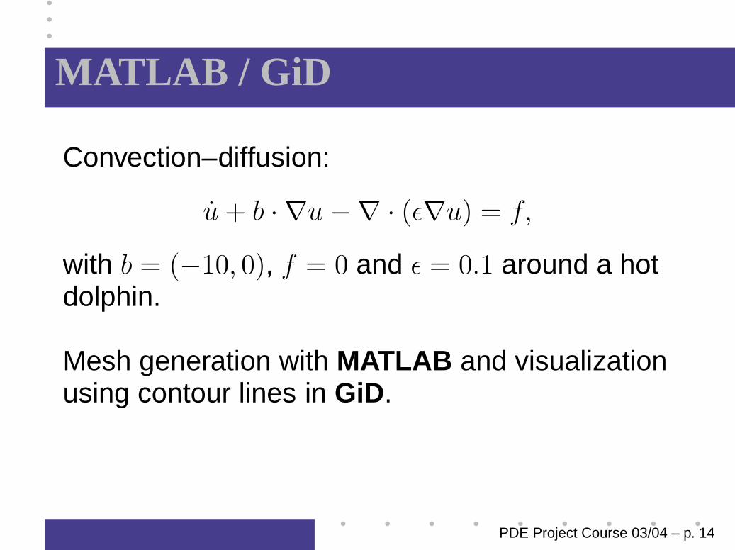
MATLAB / GiD

Convection–diffusion:

u + b · ∇u −∇ · (ε∇u) = f,

with b = (−10, 0), f = 0 and ε = 0.1 around a hotdolphin.

Mesh generation with MATLAB and visualizationusing contour lines in GiD.


MATLAB / GiD


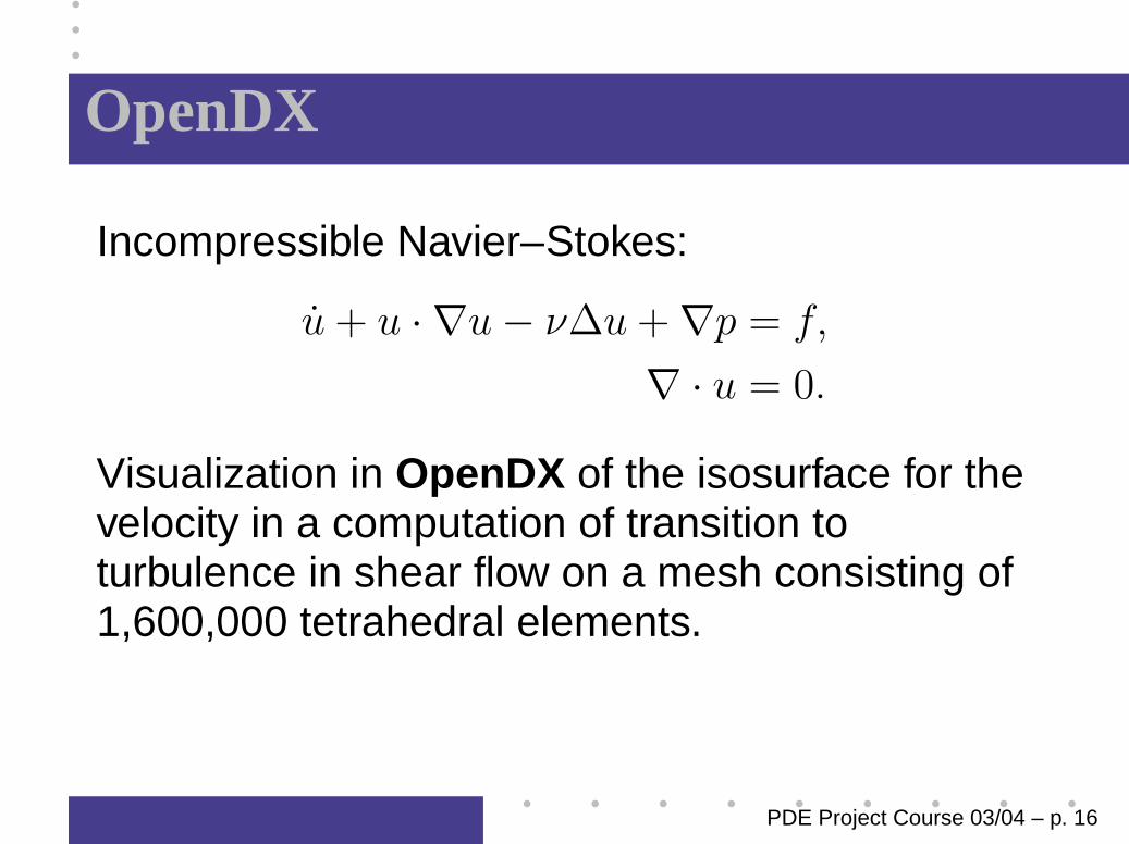
OpenDX

Incompressible Navier–Stokes:

u + u · ∇u − ν∆u + ∇p = f,

∇ · u = 0.

Visualization in OpenDX of the isosurface for thevelocity in a computation of transition toturbulence in shear flow on a mesh consisting of1,600,000 tetrahedral elements.


OpenDX


Using DOLFIN


Code structure

Tools

fem la grid quadrature

elements math common io

main.cpp

SettingsLog system

Solvers/modules

Poisson

Conv-diff

Navier-Stokes

User level

Kernel level

Module level


Three levels

• Simple C/C++ interface for the user who justwants to solve an equation with specifiedgeometry and boundary conditions.

• New algorithms are added at module level bythe developer or advanced user.

• Core features are added at kernel level.


Solving Poisson’s equation

int main()

Mesh mesh("mesh.xml.gz");

Problem poisson("poisson", mesh);

poisson.set("source", f);

poisson.set("boundary condition", mybc);

poisson.solve();

return 0;


Implementing a solver

void PoissonSolver::solve()

Galerkin fem;

Matrix A;

Vector x, b;

Function u(mesh, x);

Function f(mesh, "source");

Poisson poisson(f);

KrylovSolver solver;

File file("poisson.m");

fem.assemble(poisson, mesh, A, b);

solver.solve(A, x, b);

u.rename("u", "temperature");

file << u;


Automatic assembling

class Poisson : public PDE

...

real lhs(const ShapeFunction& u, const ShapeFunction& v)

return (grad(u),grad(v)) * dK;

real rhs(const ShapeFunction& v)

return f*v * dK;

...

;


Automatic assembling

class ConvDiff : public PDE

...

real lhs(const ShapeFunction& u, const ShapeFunction& v)

return (u*v + k*((b,grad(u))*v + a*(grad(u),grad(v))))*dK;

real rhs(const ShapeFunction& v)

return (up*v + k*f*v) * dK;

...

;


Handling meshes

Basic concepts:• Mesh

• Node, Cell, Edge, Face• Boundary

• MeshHierarchy

• NodeIteratorCellIteratorEdgeIteratorFaceIterator


Handling meshes

Reading and writing meshes:

File file(‘‘mesh.xml’’);

Mesh mesh;

file >> mesh; // Read mesh from file

file << mesh; // Save mesh to file


Handling meshes

Iteration over a mesh:

for (CellIterator c(mesh); !c.end(); ++c)

for (NodeIterator n1(c); !n1.end(); ++n1)

for (NodeIterator n2(n1); !n2.end(); ++n2)

cout << *n2 << endl;


Linear algebra

Basic concepts:

• Vector

• Matrix (sparse, dense or generic)• KrylovSolver

• DirectSolver


Linear algebra

Using the linear algebra:

int N = 100;

Matrix A(N,N);

Vector x(N);

Vector b(N);

b = 1.0;

for (int i = 0; i < N; i++)

A(i,i) = 2.0;

if ( i > 0 )

A(i,i-1) = -1.0;

if ( i < (N-1) )

A(i,i+1) = -1.0;

A.solve(x,b);


Summary of features


Summary of features

Implemented features:• Automatic assembling• Linear elements in 2D and 3D• Adaptive mesh refinement• Basic linear algebra• Solvers for Poisson and convection–diffusion• Log system• Parameter management


Summary of features

In preparation:• Multi-adaptive ODE-solver (Jansson/Logg)• Improved preconditioners

(Hoffman/Svensson)• Improved linear algebra (Hoffman/Logg)


Summary of features

Wishlist / help wanted:• Multi-grid• Implementation of boundary conditions• Eigenvalue solvers• Higher-order elements• Documentation• New solvers / modules• Testing, bug fixes


Web page

• www.phi.chalmers.se/dolfin


Overview of Puffin


Introduction

• A simple and minimal version of DOLFIN• Developed at the Department of

Computational Mathematics• Written for Octave/Matlab• Licensed under the GNU GPL• http://www.fenics.org/puffin

• Used in the computer sessions for theBody & Soul project


Using Puffin

Based around the two functionsAssembleMatrix() and AssembleVector()that are used to assemple a linear system

AU = b,

representing a variational formulation

a(u, v; w) = l(v; w) ∀v ∈ V,

where a(u, v; w) is a bilinear form in u (the trialfunction) and v (the test function), and l(v; w) is alinear form in v.


Using Puffin

A variational formulation is specified as follows:

function integral = MyForm(u, v, w, du, dv, dw, dx, ds, x, d, t, eq)

if eq == 1

integral = ... * dx + ... * ds;

else

integral = ... * dx + ... * ds;

end


Using Puffin

Example: Poissons equation.

∫Ω

∇u·∇v dx+

∫Γ

γuv ds =

∫Ω

fv dx+

∫Γ

(γgD−gN)v ds ∀v.

function integral = Poisson(u, v, w, du, dv, dw, dx, ds, x, d, t, eq)

if eq == 1

integral = du’*dv*dx + g(x,d,t)*u*v*ds;

else

integral = f(x,d,t)*v*dx + (g(x,d,t)*gd(x,d,t) - gn(x,d,t))*v*ds;

end


Using Puffin

Syntax of the function AssembleMatrix():

A = AssembleMatrix(points, edges, triangles, pde, W, time)

Syntax of the function AssembleVector():

b = AssembleVector(points, edges, triangles, pde, W, time)


Web page

• http://www.fenics.org/puffin


PDE Project Course - Chalmers

Documents

Transcript of PDE Project Course - Chalmers