
PCC Airfield Pavement Response During Thaw … Report 96-12 PCC Airfield Pavement Response During...
45
SPECIAL REPORT SPECIAL REPORT 96-12 96-12 PCC Airfield Pavement Response During Thaw-Weakening Periods A Field Study Vincent C. Janoo and Richard L. Berg May 1996
Transcript of PCC Airfield Pavement Response During Thaw … Report 96-12 PCC Airfield Pavement Response During...
SPEC
IAL
REP
OR
TSP
ECIA
L R
EPO
RT
96
-12
96
-12
PCC Airfield Pavement ResponseDuring Thaw-Weakening PeriodsA Field StudyVincent C. Janoo and Richard L. Berg May 1996
AbstractThis investigation is part of CRREL’s on-going characterization of pavementperformance in seasonal frost areas. As part of the research, CRREL conduct-ed several field studies for the Federal Aviation Administration (FAA) on theresponse of airport pavements during thaw-weakening periods at three civilairports in Wisconsin, where the design freezing index in the area was around900 to 1100°C-days and frost penetration ranged between 1250 to 2000mm. This study focused on the performance of Portland Cement Concrete(PCC) pavements during the spring thaw-weakening period. The sites wereinstrumented with subsurface thermocouples and Falling Weight Deflectome-ter (FWD) tests were conducted during the spring thaw period at the center ofthe slab and across the joints. An analysis of the FWD data and backcalcula-tion of the layer moduli using ILLIBACK and WESDEF was conducted. Uniquerelationships between the FWD deflections and the subgrade modulus andcoefficient of subgrade reaction were obtained. Additional relationships weredeveloped using the FWD deflections, PCC thickness and the horizontal ten-sile stress at the bottom of the PCC layer. A relationship between load transferacross joints and FWD deflections was also developed. On the basis of therelationships obtained in this study, a methodology for evaluating PCC pave-ments during spring thaw was developed. However, this methodology needsto be verified for other subgrade types and areas with other design freezingindices.
For conversion of SI units to non-SI units of measurement consult StandardPractice for Use of the International System of Units (SI), ASTM Standard E380-93, published by the American Society for Testing and Materials, 1916 Race St.,Philadelphia, Pa. 19103.
This report is printed on paper that contains a minimum of 50% recycledmaterial.

Special Report 96-12
PCC Airfield Pavement ResponseDuring Thaw-Weakening PeriodsA Field StudyVincent C. Janoo and Richard L. Berg May 1996
Prepared for
FEDERAL AVIATION ADMINISTRATIONand
OFFICE OF THE CHIEF OF ENGINEERS
Approved for public release; distribution is unlimited.
US Army Corps of Engineers Cold Regions Research & Engineering Laboratory

ii
PREFACE
This report was prepared by Dr. Vincent C. Janoo and Dr. Richard L. Berg, Research CivilEngineers, Civil and Geotechnical Engineering Research Division, Research and EngineeringDirectorate, U.S. Army Cold Regions Research and Engineering Laboratory. Funding was pro-vided by the Federal Aviation Administration and the Office of the Chief of Engineers. The OCEportion was funded through DA Project 4A762784 AT42, Design, Construction and OperationsTechnology for Cold Regions; Mission Area, Base Support; Work Unit BS/036, Improved Pave-ment Design Criteria in Cold Regions.
Technical review of the manuscript of this report was provided by Dr. Raymond Rollings(U.S. Army Engineer Waterways Experiment Station) and Michel Hovan (FAA). The authorsexpress special thanks to L. Barna and F. Carver for assisting in the data reduction and for theirpatience, and to R. Guyer and C. Berini for gathering the data.
The contents of this report are not to be used for advertising or promotional purposes. Citationof brand names does not constitute an official endorsement or approval of the use of such com-mercial products.
iii
CONTENTS
Preface ................................................................................................................................... iiIntroduction ........................................................................................................................... 1Description of airfields.......................................................................................................... 1
Central Wisconsin Airport ................................................................................................ 1Outagamie County Airport ............................................................................................... 3
Field instrumentation and testing program ........................................................................... 4Environmental data analysis ................................................................................................. 5FWD data analysis ................................................................................................................ 6
Bearing capacity analysis ................................................................................................. 10Backcalculation of layer moduli ...................................................................................... 14
Load transfer efficiency ........................................................................................................ 29Proposed pavement evaluation procedure ............................................................................ 37Conclusions ........................................................................................................................... 38Literature cited ...................................................................................................................... 38Abstract ................................................................................................................................. 39
ILLUSTRATIONS
Figure1. Location of airfields ....................................................................................................... 12. Pavement structure at Central Wisconsin Airport ......................................................... 23. Pavement structure at Outagamie County Airport ........................................................ 34. FWD, temperature and moisture sensor locations......................................................... 45. Daily minimum and maximum temperatures ................................................................ 56. Air-freezing indices ....................................................................................................... 67. Frost and thaw depths calculated from subsurface temperature measurements ........... 78. Location of FWD sensors across joints and corner of a PCC slab ............................... 79. Changes in basin area and impulse stiffness modulus during spring thaw at
Outagamie County Airport ....................................................................................... 1010. Changes in basin area during spring thaw at Central Wisconsin Airport ..................... 1111. Changes in impulse stiffness modulus during spring thaw at Central Wisconsin
Airport ...................................................................................................................... 1212. Relationship between surface temperature and basin area ............................................ 1313. Relationship between surface temperature and impulse stiffness modulus .................. 1414. Idealized pavement structures ........................................................................................ 1415. Effect of PCC modulus on WESDEF absolute error, Outagamie County Airport ....... 1516. Effect of PCC modulus on change in subgrade modulus from WESDEF during
spring thaw at Outagamie County Airport ............................................................... 1617. Backcalculated base course modulus using WESDEF, Outagamie County Airport ..... 1718. Change in subgrade modulus during spring thaw ......................................................... 1819. Change in base course modulus during spring thaw ..................................................... 1920. Relationship between subgrade moduli backcalculated by WESDEF and ILLIBACK . 2021. Typical backcalculated PCC modulus from ILLIBACK ............................................... 2022. Relationship between measured total basin area and calculated subgrade modulus .... 2123. Relationship between measured partial basin area and calculated subgrade modulus
at Outagamie County Airport ................................................................................... 2124. Relationship between measured impulse stiffness modulus and calculated subgrade
modulus .................................................................................................................... 22

iv
Figure25. Relationship between total basin area and subgrade modulus at Central Wisconsin
Airport and Outagamie County Airport ................................................................... 2226. Relationship between total basin area and coefficient of subgrade reaction calcu-
lated using ILLIBACK at Outagamie County Airport and Central WisconsinAirport ...................................................................................................................... 23
27. Relationship between impulse stiffness modulus and subgrade modulus atOutagamie County Airport and Central Wisconsin Airport .................................... 24
28. Configuration and location of stress calculations for Boeing 757 and MD-DC9 ......... 2529. Amount of damage during spring thaw at Central Wisconsin Airport .......................... 2530. Effect of pavement thickness on damage at Central Wisconsin Airport ....................... 2531. Amount of damage during spring thaw at Outagamie County Airport ......................... 2732. Effect of subgrade modulus on the horizontal tensile stress at the bottom of the PCC
layer at Outagamie County Airport and Central Wisconsin Airport ....................... 2733. Effect of the coefficient of subgrade reaction on the horizontal tensile stress at the
bottom of the PCC layer .......................................................................................... 2834. Effect of PCC modulus on the horizontal tensile stress at the bottom of the PCC
layer .......................................................................................................................... 2935. Linear relationship between total basin area and maximum horizontal tensile stress
at bottom of PCC layer ........................................................................................... 3036. Relationship between impulse stiffness modulus and horizontal tensile stress at
bottom of PCC layer ................................................................................................ 3037. Load transfer efficiency across a joint ........................................................................... 3038. Placement of FWD sensors for load transfer efficiency test ......................................... 3139. Relationship between air temperature and transverse joint transfer efficiency ............ 3140. Change of transverse joint efficiency with subsurface temperature ............................. 3441. Effect of subgrade modulus calculated with ILLIBACK on transverse joint
efficiency .................................................................................................................. 3442. Change in transverse joint transfer with time on taxiway B, Central Wisconsin
Airport ...................................................................................................................... 3543. Relationship between AREA and l for a dense liquid foundation ................................ 3544. Interpolated relationships between joint efficiency and load transfer as a function
of a / l ........................................................................................................................ 3645. Relationship between JTE and LTE for transverse joints ............................................. 3646. Relationship between total basin area and subgrade modulus ...................................... 3747. Relationship between JTE and LTE............................................................................... 37
TABLES
Table1. Pavement structures at Central Wisconsin Airport ........................................................ 22. Temperature sensor locations under pavement surface ................................................. 43. Types of falling weight deflection tests conducted ....................................................... 84. Pavement surface temperatures at time of falling weight deflection test ..................... 95. Thickness of subgrade at backcalculated falling weight deflection locations .............. 156. Backcalculated modulus at Central Wisconsin Airport using WESDEF....................... 177. Effect of change in PCC modulus on base and subgrade modulus ............................... 188. Gear loading for the MD-DC9 and Boeing 757 ............................................................ 249. Gear information for computer simulations of the MD-DC9 and Boeing 757 ............. 24
10. Ratio of maximum horizontal tensile stress to flexural strength during spring thaw ... 2611. Joint transfer efficiencies at Central Wisconsin Airport ................................................ 3212. Joint transfer efficiencies at Outagamie County Airport ............................................... 33

INTRODUCTION
In the spring of 1986, CRREL conducted a fieldstudy for the Federal Aviation Administration (FAA)on how airport pavements responded to frost action.The emphasis was on thaw weakening. The study wasconducted at three regional airports in Wisconsin—Central Wisconsin Airport (CWA), Outagamie CountyAirport (OCA) and Wittman Field. The pavement sur-faces at CWA and OCA were predominately PortlandCement Concrete (PCC), whereas at Wittman theywere mostly Asphalt Concrete (AC). The results of astudy on AC airfield pavement structures during thaw-weakening periods can be found in a previously pub-lished report (Janoo and Berg 1991). This report exam-ines PCC airport pavements during thaw periods.
It is accepted that in the winter the load carryingcapacity of pavements increases dramatically becauseof freezing of the pavement structure. This is more dra-matic in AC pavements because of the stiffening of theasphalt at low temperatures. This increase is also seenin PCC pavements because of a similar stiffening ofthe base, subbase and subgrade.
During thaw periods, the pavement structure belowthe PCC layer thaws and can become saturated withwater from the melting ice lenses and infiltration ofsurface water from rain or melting snow. This satura-tion of the material reduces the strength of the base,subbase or subgrade, or all three, leading to reducedbearing capacity of the entire pavement structure. Inaddition, the large temperature differentials duringthawing periods can cause curling of the corners andedges of slabs of PCC pavements, thus affecting loadtransfer across joints.
The objective of the study was to determine anystructural changes in PCC airport pavements duringthaw-weakening periods. To evaluate these changes,CRREL conducted Falling Weight Deflectometer(FWD) measurements to quantify the changes in thestiffness of the pavement structure and the load trans-fer efficiency of the joints. In addition, subsurface
PCC Airfield Pavement ResponseDuring Thaw-Weakening Periods
A Field Study
VINCENT C. JANOO AND RICHARD L. BERG
pavement temperatures were measured at selected lo-cations at each airport. This report gives a general de-scription of the airports and the pavement structuresand a comprehensive analysis of the FWD measure-ments.
DESCRIPTION OF AIRFIELDS
Central Wisconsin Airport (CWA)CWA is located in Mosinee, Wisconsin (Fig. 1).
The subsurface soils at CWA are silts, sandy silts andclayey silts and can be classified as either SM or MLusing the Unified Soil Classification System, and asF3 and F4 with respect to frost-susceptibility (Starkand Berg 1989). F3 and F4 soils are very susceptibleto frost heave and thaw weakening. Stark and Berg(1989) also reported that the subgrade was not uni-
Figure 1. Location of airfields.
* Mean Air Freezing Index (°C-days)
CWAMosinee
AppletonOCA

2
Figure 2. Pavement structure at Central Wisconsin Airport (CWA).
Table 1. Pavement structures at Central Wisconsin Airport.
SlabDate Length Width size Longitudinal Transverse
Pavement constructed (m) (m) (m) joint joint
Runway 8/26(original) 1968 2042 46 3.8 × 6.1 keyed & dummy doweled
Runway 8/26(extension) 1973 244 46 7.6 × 7.6 keyed doweled
Runway 17/35 1972 1737 46 7.6 × 7.6 keyed doweled
Taxiway A 1969 297 23 3.8 × 6.1 keyed & tied doweled
Taxiway B(ramp to taxiway C) 1975 139 23 7.6 × 7.6 keyed & tied doweled
3.8 × 7.6Taxiway B(taxiway C to 17/35) 1977 954 15 3.8 × 7.6 Butt, tied doweled & dummy
Taxiway C 1973 2256 15 7.6 × 7.6 keyed & tied doweled3.8 × 7.6
Taxiway D 1973 88 20 7.6 × 7.6 keyed & tied doweled3.8 × 7.6
Taxiway E 1973 88 20 3.8 × 5.3 keyed & tied doweled
form, having clusters of rocks and boulders incor-porated into the finer grained soils. Bedrock was re-ported at uneven depths and at some locations it wasclose to the pavement surface.
The airport pavements consist of two intersectingrunways, five taxiways and three ramps (Fig. 2). Theoriginal airfield—runway 8/26, taxiway A and an aircarrier ramp—was constructed in 1968 and 1969. Be-tween 1972 and 1973, runway 17/35 and taxiways C,D and E were constructed. Also in 1973, runway 8/26
was extended by 245 m and the air carrier ramp ex-panded. Taxiway B (between the ramp and taxiway C)was constructed in 1975 and was extended to connectthe two runways in 1977. Portions of runway 8/26were reconstructed in 1987. A summary of the con-struction history, length, width and types of joints ofthe different pavement structures at CWA is presentedin Table 1.
The airfield basically was constructed with PCC.The original runway, taxiway and ramp, constructed

in 1968 and 1969, had 254 mm of PCC over 229 mmof crushed stone base over subgrade. Later construc-tion mostly used 305 mm of PCC over 229 mm ofcrushed stone base over subgrade. The structure of thedifferent pavement sections as of spring 1986 is alsoshown in Figure 2.
The slabs sizes were primarily 7.6 by 7.6 m; how-ever, in some areas, the slabs were 3.8 by 3.8 m. Othersizes used are shown in Table 1. Loads are transferredacross the transverse joints by dowels and aggregateinterlocks (Table 1) (CMT 1984). At longitudinaljoints, loads are transferred through keyways, aggre-gate interlocks and tiebars (Table 1) (CMT 1984). Theprimary types of aircraft using the airport are Convair580 (24,766 kg), MD DC-9 (44,452 kg) and Boeing757 (115,666 kg) (CMT 1984).
Outagamie County Airport (OCA)OCA is located near Appleton, Wisconsin (Fig. 1).
The subgrade at the airport consists mostly of a lowplasticity clay (CL), some sand (SP) and silty sand(SM). At OCA, bedrock was estimated to be 4.0 mdeep or more, on the basis of boring logs. ERES con-sultants (1985) reported the subgrade under runway3/21 as a highly frost-susceptible red silty clay. Theyalso reported that the subbase material may be frost-susceptible because of a high amount of fines passingthe no. 200 sieve (8–10 %). Runway 3/21 has severefrost heave problems (ERES 1985). Mead and Hunt(1988) reported that the subgrade under runway 11/29
was a heavy clay (USC classification–CL; FAA clas-sification–E7) with a design California Bearing Ratio(CBR) of 4. They also reported clay migration into thebase course and trapped water under the pavement.
The airport pavements consist of two intersectingrunways, five taxiways and three ramps (Fig. 3). Run-way 3/21 was constructed in 1967 and 1968, with 203mm of PCC (254 mm in critical areas) over 203 mm ofcrushed gravel over subgrade. Runway 11/29, recon-structed in 1988 and 1989, had 178 mm PCC (229 mmin critical areas) over 203 mm of crushed aggregatebase course over subgrade.
The PCC slabs were mostly 3.8 m wide by 6.1 mlong; but, in some areas, the slabs were 3.8 m wide by5.3 m long. A typical transverse joint used aggregateinterlocks and dowels for load transfer.* Across longi-
tudinal joints, keyways, aggregate interlocks and tie-bars were used for load transfer (ERES Consultants1985, Mead and Hunt 1988). Richardson stated thaton the basis of a pavement evaluation done prior to1986, the gross allowable aircraft weights on runway11/29 were 27,200-kg single, 40,800-kg dual and74,860-kg dual tandem. On runway 3/21, the gross al-lowable aircraft weights were 38,570-kg single,81,670-kg dual and 95,280-kg dual tandem.
3
Figure 3. Pavement structure at Outagamie County Airport (OCA).
N
3
29
T/W
E
T/W C
T/W B
Runway 3-21
Runw
ay 11-29
T/W D
21
T/W
A11
Outagamie County Airport
Base
200 mm Gravel203 mm Gravel200 mm Gravel203 mm Gravel
Surface
178 mm PCC203 mm PCC229 mm PCC254 mm PCC
* Personal Communication, with K. Richardson, Wisconsin De-partment of Transportation, 1991.

FIELD INSTRUMENTATIONAND TESTING PROGRAM
In the summer of 1985, several locations along theairport runways and taxiways were instrumented withmoisture sensors and copper-constantan thermocouplesas temperature sensors. At CWA, six locations were in-strumented for temperature measurement (Fig. 4a). AtOCA, there were two temperature measurement sites(Fig. 4b). With a few exceptions, thermocouples wereplaced to depths of approximately 5 m below the pave-ment surface. The spacings of the sensors are given inTable 2. At TC4, the hole could not be held open past2.5 m from the surface.
The temperature measurements were made periodi-cally by airport personnel during the winter months andby CRREL personnel during the FWD testing period inthe spring. The measured temperatures at the two air-ports are given in Janoo and Berg (1996).
In the spring of 1986, non-destructive testing using aDynatest 8000 Falling Weight Deflectometer (FWD)
4
b. Outagamie County Airport.
Table 2. Temperature sensor locations under pave-ment surface (cm).
Sensor TC1, TC2 (CWA)no. TC1, TC2 (OCA) TC3 (CWA) TC4 (CWA)
1 30.5 30.5 30.52 45.7 45.7 45.73 61 106.7 614 91.4 137.2 91.45 121.9 167.6 121.96 152.4 198.1 152.47 182.9 228.6 182.98 213.4 259.1 213.49 243.8 289.6 243.8
10 304.8 350.5 259.111 365.8 411.5 137.212 487.7 472.4 106.7
a. Central Wisconsin Airport.
Figure 4. FWD, temperature and moisture sensor locations.
was conducted at selected sites at the two airports.The FWD test sites covered a large area of the airportsand included both AC and PCC pavements. As men-tioned earlier, the analysis presented here is for onlythe PCC slabs. Deflection measurements were made
5
a. Central Wisconsin Airport.
Tem
pera
ture
(C
)
–40
–20
0
20
40
20 Sep 20 Oct 19 Nov 19 Dec 18 Jan 17 Feb 19 Mar 18 Apr 18 May
Outagamie County Airport, Appleton
Maximum
Minimum
1985 1986
b. Outagamie County Airport, Appleton.
Figure 5. Daily maximum and minimum temperatures.
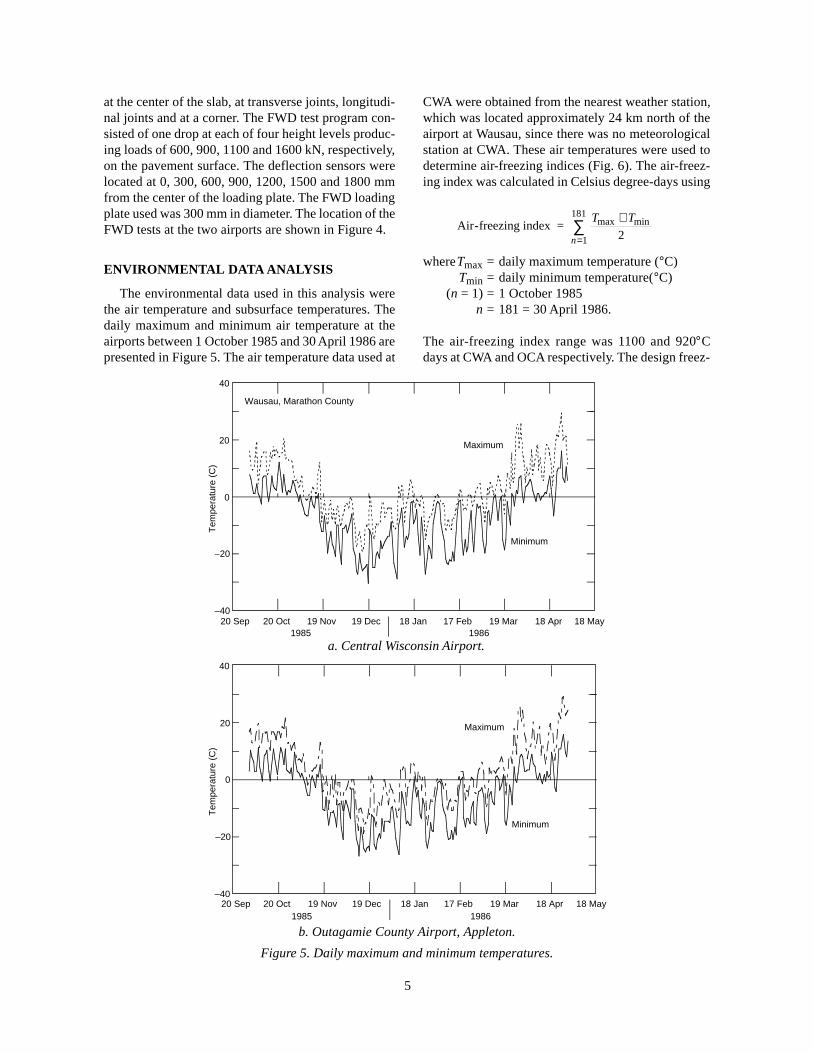
at the center of the slab, at transverse joints, longitudi-nal joints and at a corner. The FWD test program con-sisted of one drop at each of four height levels produc-ing loads of 600, 900, 1100 and 1600 kN, respectively,on the pavement surface. The deflection sensors werelocated at 0, 300, 600, 900, 1200, 1500 and 1800 mmfrom the center of the loading plate. The FWD loadingplate used was 300 mm in diameter. The location of theFWD tests at the two airports are shown in Figure 4.
ENVIRONMENTAL DATA ANALYSIS
The environmental data used in this analysis werethe air temperature and subsurface temperatures. Thedaily maximum and minimum air temperature at theairports between 1 October 1985 and 30 April 1986 arepresented in Figure 5. The air temperature data used at
CWA were obtained from the nearest weather station,which was located approximately 24 km north of theairport at Wausau, since there was no meteorologicalstation at CWA. These air temperatures were used todetermine air-freezing indices (Fig. 6). The air-freez-ing index was calculated in Celsius degree-days using
Air-freezing index = T T
n
max min+
=∑
21
181
whereTmax = daily maximum temperature (°C)Tmin = daily minimum temperature(°C)
(n = 1) = 1 October 1985n = 181 = 30 April 1986.
The air-freezing index range was 1100 and 920°Cdays at CWA and OCA respectively. The design freez-
Tem
pera
ture
(C
)
–40
–20
0
20
40
20 Sep 20 Oct 19 Nov 19 Dec 18 Jan 17 Feb 19 Mar 18 Apr 18 May
Wausau, Marathon County
Maximum
Minimum
1985 1986
6
Air
Fre
ezin
g In
dex
(°C
deg
ree-
days
)
–800
–400
0
400
30 Sep 30 Oct 29 Nov 29 Dec 28 Jan 27 Feb 29 Mar 28 Apr 28 May
CWA, Mosinee
Beginning of Freezing Period (17 Nov)
Beginning of Spring Thaw (29 Mar)
Air Freezing Index (1100 °C degree-days)
1985 1986
Air
Fre
ezin
g In
dex
(°C
deg
ree-
days
)
–800
–400
0
400
30 Sep 30 Oct 29 Nov 29 Dec 28 Jan 27 Feb 29 Mar 28 Apr 28 May
Appleton
Beginning of Freezing Period (19 Nov)
Beginning of Spring Thaw (24 Mar)
Air Freezing Index (920 °C degree-days)
1985 1986
a. Central Wisconsin Airport.
b. Outagamie County Airport.
Figure 6. Air-freezing indices.
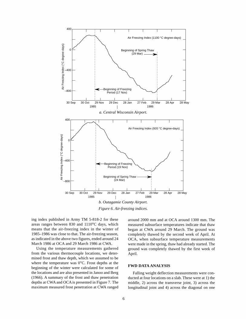
ing index published in Army TM 5-818-2 for theseareas ranges between 830 and 1110°C days, whichmeans that the air-freezing index in the winter of1985–1986 was close to that. The air-freezing season,as indicated in the above two figures, ended around 24March 1986 at OCA and 29 March 1986 at CWA.
Using the temperature measurements gatheredfrom the various thermocouple locations, we deter-mined frost and thaw depth, which we assumed to bewhere the temperature was 0°C. Frost depths at thebeginning of the winter were calculated for some ofthe locations and are also presented in Janoo and Berg(1966). A summary of the frost and thaw penetrationdepths at CWA and OCA is presented in Figure 7. Themaximum measured frost penetration at CWA ranged
around 2000 mm and at OCA around 1300 mm. Themeasured subsurface temperatures indicate that thawbegan at CWA around 29 March. The ground wascompletely thawed by the second week of April. AtOCA, when subsurface temperature measurementswere made in the spring, thaw had already started. Theground was completely thawed by the first week ofApril.
FWD DATA ANALYSIS
Falling weight deflection measurements were con-ducted at four locations on a slab. These were at 1) themiddle, 2) across the transverse joint, 3) across thelongitudinal joint and 4) across the diagonal on one

7
0
500
1000
1500
2000
250029 Nov '85 29 Dec 28 Jan '86 27 Feb 29 Mar 28 Apr 28 May
Fro
st D
epth
(m
m)
TC1TC2TC4TC6
a. Central Wisconsin Airport.0
500
1000
1500
200029 Nov '85 29 Dec 28 Jan '86 27 Feb 29 Mar 28 Apr
Fro
st D
epth
(m
m)
Assumed
TC1TC2
b. Outagamie County Airport.
Figure 7. Frost and thaw depths calculated from subsurface temperature measurements.
Transverse Joint
Corner Joint
Directionof Travel
LongitudinalJoint
D1
D0D0
D1 D0
D1
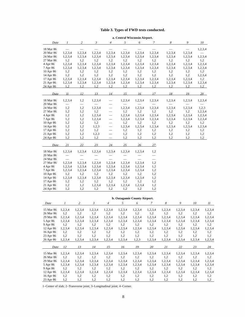
corner of the slab. The placement of the sensors acrossthe joints and corner is illustrated in Figure 8. TheFWD measurements were alternated between the twoairports. At CWA, FWD deflection measurements be-gan on 18 March and continued to 24 April 1986 (Table3a). At OCA, FWD testing started on 15 March andcontinued to 26 April 1986 (Table 3b). The FWD de-flection measurements taken at both airports are pre-sented in Janoo and Berg (1966).
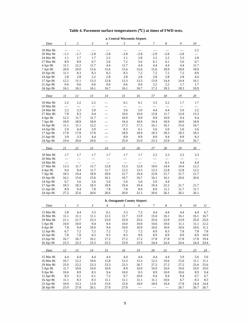
The pavement surface temperatures at the time ofFWD testing for both airports are presented in Table 4.Surface temperatures were measured with a thermo-couple attached to a wooden dowel. The thermocouplewas placed against the pavement by the FWD operator.At the time of FWD testing, the pavement surface atCWA was dry except on 18 March and 14 April. AtOCA, the pavement surface was dry except on 5 April.Subsurface temperature measurements indicated thatthe pavement structures at CWA were frozen at the be-ginning of FWD testing and completely thawed by the
Figure 8. Location of FWD sensors across joints andcorner of a PCC slab.
8
Table 3. Types of FWD tests conducted.
a. Central Wisconsin Airport.
Date 1 2 3 4 5 6 7 8 9 10
18 Mar 86 — — — — — — — — — 1,2,3,420 Mar 86 1,2,3,4 1,2,3,4 1,2,3,4 1,2,3,4 1,2,3,4 1,2,3,4 1,2,3,4 1,2,3,4 1,2,3,4 —24 Mar 86 1,2,3,4 1,2,3,4 1,2,3,4 1,2,3,4 1,2,3,4 1,2,3,4 1,2,3,4 1,2,3,4 1,2,3,4 1,2,3,427 Mar 86 1,2 1,2 1,2 1,2 1,2 1,2 1,2 1,2 1,2 1,24 Apr 86 1,2,3,4 1,2,3,4 1,2,3,4 1,2,3,4 1,2,3,4 1,2,3,4 1,2,3,4 1,2,3,4 1,2,3,4 1,2,3,47 Apr 86 1,2,3,4 1,2,3,4 1,2,3,4 1,2,3,4 1,2,3,4 1,2,3,4 1,2,3,4 1,2,3,4 1,2,3,4 1,2,3,410 Apr 86 1,2 1,2 1,2 1,2 1,2 1,2 1,2 1,2 1,2 1,214 Apr 86 1,2 1,2 1,2 1,2 1,2 1,2 1,2 1,2 1,2 1,2,3,417 Apr 86 1,2,3,4 1,2,3,4 1,2,3,4 1,2,3,4 1,2,3,4 1,2,3,4 1,2,3,4 1,2,3,4 1,2,3,4 1,221 Apr 86 1,2,3,4 1,2,3,4 1,2,3,4 1,2,3,4 1,2,3,4 1,2,3,4 1,2,3,4 1,2,3,4 1,2,3,4 1,2,3,424 Apr 86 1,2 1,2 1,2 1,2 1,2 1,2 1,2 1,2 1,2 1,2
Date 11 12 13 14 15 16 17 18 19 20
18 Mar 86 1,2,3,4 1,2 1,2,3,4 — 1,2,3,4 1,2,3,4 1,2,3,4 1,2,3,4 1,2,3,4 1,2,3,420 Mar 86 — — — — — — — — — —24 Mar 86 1,2 1,2 1,2,3,4 — 1,2,3,4 1,2,3,4 1,2,3,4 1,2,3,4 1,2,3,4 1,2,327 Mar 86 1,2 1,2 1,2 — 1,2 1,2 1,2 1,2 1,2 1,2,3,44 Apr 86 1,2 1,2 1,2,3,4 — 1,2,3,4 1,2,3,4 1,2,3,4 1,2,3,4 1,2,3,4 1,2,3,47 Apr 86 1,2 1,2 1,2,3,4 — 1,2,3,4 1,2,3,4 1,2,3,4 1,2,3,4 1,2,3,4 1,2,3,410 Apr 86 1,2 1,2 1,2 — 1,2 1,2 1,2 1,2 1,2 1,214 Apr 86 1,2 1,2 1,2,3 — 1,2,3,4 1,2,3,4 1,2,3,4 1,2,3,4 1,2,3,4 1,2,3,417 Apr 86 1,2 1,2 1,2 — 1,2 1,2 1,2 1,2 1,2 1,221 Apr 86 1,2 1,2 1,2,3 — 1,2 1,2 1,2 1,2 1,2 1,224 Apr 86 1,2 1,2 1,2 — 1,2 1,2 1,2 1,2 1,2 1,2
Date 21 22 23 24 25 26 27
18 Mar 86 1,2,3,4 1,2,3,4 1,2,3,4 1,2,3,4 1,2,3,4 1,2,3,4 1,220 Mar 86 — — — — — — —24 Mar 86 — — — — — — —27 Mar 86 1,2,3,4 1,2,3,4 1,2,3,4 1,2,3,4 1,2,3,4 1,2,3,4 1,24 Apr 86 1,2,3,4 1,2,3,4 1,2,3,4 1,2,3,4 1,2,3,4 1,2,3,4 1,27 Apr 86 1,2,3,4 1,2,3,4 1,2,3,4 1,2,3,4 1,2,3,4 1,2,3,4 1,210 Apr 86 1,2 1,2 1,2 1,2 1,2 1,2 1,214 Apr 86 1,2,3,4 1,2,3,4 1,2,3,4 1,2,3,4 1,2,3,4 1,2,3,4 1,217 Apr 86 1,2 1,2 1,2 1,2 1,2 1,2 1,221 Apr 86 1,2 1,2 1,2,3,4 1,2,3,4 1,2,3,4 1,2,3,4 1,224 Apr 86 1,2 1,2 1,2 1,2 1,2 1,2 1,2
b. Outagamie County Airport.
Date 1 2 3 4 5 6 7 8 9 10 11
15 Mar 86 1,2,3,4 1,2,3,4 1,2,3,4 1,2,3,4 1,2,3,4 1,2,3,4 1,2,3,4 1,2,3,4 1,2,3,4 1,2,3,4 1,2,3,426 Mar 86 1,2 1,2 1,2 1,2 1,2 1,2 1,2 1,2 1,2 1,2 1,229 Mar 86 1,2,3,4 1,2,3,4 1,2,3,4 1,2,3,4 1,2,3,4 1,2,3,4 1,2,3,4 1,2,3,4 1,2,3,4 1,2,3,4 1,2,3,45 Apr 86 1,2,3,4 1,2,3,4 1,2,3,4 1,2,3,4 1,2,3,4 1,2,3,4 1,2,3,4 1,2,3,4 1,2,3,4 1,2,3,4 1,2,3,49 Apr 86 1,2 1,2 1,2 1,2 1,2 1,2 1,2 1,2 1,2 1,2 1,212 Apr 86 1,2,3,4 1,2,3,4 1,2,3,4 1,2,3,4 1,2,3,4 1,2,3,4 1,2,3,4 1,2,3,4 1,2,3,4 1,2,3,4 1,2,3,416 Apr 86 1,2 1,2 1,2 1,2 1,2 1,2 1,2 1,2 1,2 1,2 1,223 Apr 86 1,2 1,2 1,2 1,2 1,2 1,2 1,2 1,2 1,2 1,2 1,226 Apr 86 1,2,3,4 1,2,3,4 1,2,3,4 1,2,3,4 1,2,3,4 1,2,3 1,2,3,4 1,2,3,4 1,2,3,4 1,2,3,4 1,2,3,4
Date 12 13 14 15 16 19 20 21 22 23 24
15 Mar 86 1,2,3,4 1,2,3,4 1,2,3,4 1,2,3,4 1,2,3,4 1,2,3,4 1,2,3,4 1,2,3,4 1,2,3,4 1,2,3,4 1,2,3,426 Mar 86 1,2 1,2 1,2 1,2 1,2 1,2 1,2 1,2 1,2 1,2 1,229 Mar 86 1,2,3,4 1,2,3,4 1,2,3,4 1,2,3,4 1,2,3,4 1,2,3,4 1,2,3,4 1,2,3,4 1,2,3,4 1,2,3,4 1,2,3,45 Apr 86 1,2,3,4 1,2,3,4 1,2,3,4 1,2,3,4 1,2,3,4 1,2,3,4 1,2,3,4 1,2,3,4 1,2,3,4 1,2,3,4 1,2,3,49 Apr 86 1,2 1,2 1,2 1,2 1,2 1,2 1,2 1,2 1,2 1,2 1,212 Apr 86 1,2,3,4 1,2,3,4 1,2,3,4 1,2,3,4 1,2,3,4 1,2,3,4 1,2,3,4 1,2,3,4 1,2,3,4 1,2,3,4 1,2,3,416 Apr 86 1,2 1,2 1,2 1,2 1,2 1,2 1,2 1,2 1,2 1,2 1,223 Apr 86 1,2 1,2 1,2 1,2 1,2 1,2 1,2 1,2 1,2 1,2 1,2
1–Center of slab; 2–Transverse joint; 3–Longitudinal joint; 4–Corner.
9
Table 4. Pavement surface temperatures (°°°°°C) at times of FWD tests.
a. Central Wisconsin Airport.
Date 1 2 3 4 5 6 7 8 9 10
18 Mar 86 — — — — — — — — — 2.220 Mar 86 –1.1 –1.7 –2.8 –2.8 –2.8 –2.8 –2.8 –2.8 –2.8 —24 Mar 86 1.1 1.7 1.7 2.2 1.1 2.8 2.2 2.2 3.3 2.827 Mar 86 8.9 8.9 6.7 5.6 7.2 5.6 6.1 6.1 5.0 6.74 Apr 86 11.1 12.2 11.7 4.4 11.7 4.4 4.4 4.4 4.4 11.77 Apr 86 20.0 20.0 15.6 15.6 15.6 15.6 15.6 18.9 18.9 18.910 Apr 86 11.1 8.3 8.3 8.3 8.3 7.2 7.2 7.2 7.2 8.914 Apr 86 2.8 2.8 2.2 2.8 2.8 2.8 2.8 2.8 2.8 4.417 Apr 86 12.2 11.1 13.3 12.8 13.3 13.3 13.9 14.4 14.4 16.121 Apr 86 0.6 0.6 0.6 0.6 0.6 0.6 2.2 2.2 1.7 1.724 Apr 86 16.1 16.1 16.1 16.7 16.1 16.7 17.2 18.3 18.3 18.9
Date 11 12 13 14 15 16 17 18 19 20
18 Mar 86 2.2 2.2 2.2 — 6.1 6.1 3.3 2.2 1.7 1.720 Mar 86 — — — — — — — — — —24 Mar 86 2.2 3.3 3.9 — 5.6 5.0 4.4 4.4 5.0 2.227 Mar 86 7.8 8.3 9.4 — 10.0 10.0 12.8 11.7 12.8 13.34 Apr 86 12.2 11.7 11.7 — 10.0 8.9 8.9 10.0 9.4 9.47 Apr 86 18.9 18.9 18.9 — 19.4 18.9 19.4 18.9 18.9 18.910 Apr 86 11.1 11.1 12.2 — 17.2 17.2 16.1 16.1 15.6 16.714 Apr 86 5.0 4.4 3.9 — 8.3 6.1 5.6 5.0 5.0 5.617 Apr 86 17.8 17.8 17.8 — 18.9 18.9 18.3 18.3 18.3 18.321 Apr 86 3.9 3.3 4.4 — 8.9 8.9 8.9 9.4 8.9 8.324 Apr 86 19.4 20.0 20.6 — 25.0 25.0 23.3 23.9 25.6 26.7
Date 21 22 23 24 25 26 27 28 29 30
18 Mar 86 1.7 1.7 1.7 1.7 1.7 1.7 2.2 3.3 3.3 3.320 Mar 86 — — — — — — — — — —24 Mar 86 — — — — — — — 6.1 4.4 4.427 Mar 86 13.3 11.7 11.7 12.8 13.3 12.8 10.0 14.4 14.4 12.24 Apr 86 9.4 9.4 11.7 11.7 12.2 13.3 13.3 12.8 12.8 12.27 Apr 86 18.3 19.4 18.9 20.0 21.7 19.4 22.8 21.7 21.7 21.710 Apr 86 16.1 15.6 15.6 16.1 16.7 16.7 16.1 16.1 20.6 20.614 Apr 86 6.7 5.6 5.6 5.6 5.6 5.6 5.0 4.417 Apr 86 18.3 18.3 18.3 18.9 19.4 19.4 19.4 22.2 21.7 21.721 Apr 86 8.9 9.4 7.8 7.8 7.8 8.9 8.9 11.1 11.7 11.724 Apr 86 27.2 25.6 20.6 20.6 20.0 21.1 20.6 26.1 26.1 26.1
b. Outagamie County Airport.
Date 1 2 3 4 5 6 7 8 9 10 11
15 Mar 86 2.8 4.4 3.3 6.1 3.3 7.2 4.4 4.4 4.4 4.4 6.726 Mar 86 11.1 11.1 11.1 12.2 11.7 13.9 15.6 16.1 16.1 16.1 16.729 Mar 86 21.1 21.7 23.3 23.9 23.9 25.6 25.6 23.9 23.9 25.0 25.05 Apr 86 10.0 10.0 9.4 9.4 10.0 10.0 10.6 10.6 11.1 11.1 12.29 Apr 86 7.8 9.4 10.0 9.4 10.0 10.0 10.6 10.6 10.6 10.6 11.112 Apr 86 6.7 7.2 7.2 7.2 7.2 7.2 8.9 8.3 7.8 7.8 7.816 Apr 86 7.8 7.8 8.3 8.3 8.3 8.9 8.9 8.9 8.9 8.9 10.023 Apr 86 16.7 16.7 16.1 17.2 17.2 17.2 17.8 17.8 17.8 17.8 19.426 Apr 86 23.3 23.3 23.3 23.3 23.9 23.9 24.4 24.4 24.4 24.4 24.4
Date 12 13 14 15 16 19 20 21 22 23 24
15 Mar 86 4.4 4.4 4.4 4.4 4.4 4.4 4.4 4.4 3.9 5.6 5.626 Mar 86 16.7 12.2 10.6 12.8 13.3 13.3 12.2 10.6 15.6 11.1 11.129 Mar 86 25.0 22.2 23.3 23.3 23.3 26.7 27.2 27.2 27.2 25.6 25.65 Apr 86 11.7 10.6 10.0 10.0 8.9 10.0 10.0 10.0 10.6 10.0 10.09 Apr 86 10.6 8.9 8.3 9.4 10.0 8.3 8.9 10.0 10.6 8.9 9.412 Apr 86 8.3 6.1 6.1 7.2 6.7 10.0 9.4 9.4 9.4 6.7 6.716 Apr 86 11.1 8.3 8.3 11.1 11.1 11.1 11.1 10.6 6.7 8.3 8.323 Apr 86 18.9 13.3 13.9 15.0 15.0 18.9 18.9 19.4 17.8 14.4 14.426 Apr 86 25.0 27.8 26.1 27.8 27.8 — — — 26.7 26.7 26.7

end. At OCA the subsurface temperature measure-ments indicated that the pavement structures werepartially thawed at the beginning of FWD testing andcompletely thawed prior to the end. It should be notedthat no FWD data were obtained during the 6-day pe-riod from 29 March through 4 April, which was un-doubtedly the critical thaw-weakening period. Thiswas unfortunate; however, we will work with the datathat we have.
Bearing capacity analysisAny change in the structural capacity of the pave-
ment during the thaw-weakening period was inferredfrom the FWD data. We used both the deflection basin
10
Figure 9. Changes in basin area and impulse stiffness modulus during spring thaw at Outagamie County Airport.
b. Change in ISM.
FWD 3FWD 7FWD 22FWD 23FWD 24
30
20
10
0
1000
800
600
400
200
010 Mar 15 20 25 30 4 Apr 9 14 19 24 29
ISM
(M
N/m
)
Tem
pera
ture
(°C
)
Outagamie County Airport
a. Change in basin area.
area concept and the Impulse Stiffness Modulus(ISM) to characterize the changes in pavement perfor-mance. The basin area method was a good indicator ofAC pavement response during thaw periods undercontrolled conditions (Janoo and Berg 1990, 1991).The deflection basin obtained from the seven-deflec-tion sensor system is used to calculate the basin areaby the following equation
Basin Area i i+1 i+1 i= +( ) −( )[ ]=∑1
2 0
6δ δ r r
i
where δi is deflection at sensor (i), and r i is sensor (i)distance from the center of the loading plate.
1000
800
600
400
200
010 Mar 15 20 25 30 4 Apr 9 14 19 24 29
30
20
10
0
Bas
in A
rea
(mm
)2
Tem
pera
ture
(°C
)
Outagamie County Airport
FWD 3FWD 7FWD 22FWD 23FWD 24
11
400
300
200
100
014 Mar 19 24 29 3 Apr 8 13 18 23 28 3 May
Temperature
Loc 3
Central Wisconsin Airport 20
10
0 Sur
face
Tem
pera
ture
(°C
)
Bas
in A
rea
(mm
)
2
400
600
200
014 Mar 19 24 29 3 Apr 8 13 18 23 28 3 May
Temperature
Central Wisconsin Airport
20
10
0 Sur
face
Tem
pera
ture
(°C
)
Bas
in A
rea
(mm
)
2
Loc 2Loc 6Loc 9
400
600
200
014 Mar 19 24 29 3 Apr 8 13 18 23 28
Central Wisconsin Airport
Bas
in A
rea
(mm
)
2
30
20
10
0
Sur
face
Tem
pera
ture
(°C
)
Temperature
Loc 15Loc 16Loc 17Loc 18Loc 19
b. FWD locations 2, 6 and 9.
a. FWD location 3 .
c. FWD locations 15 to 19.
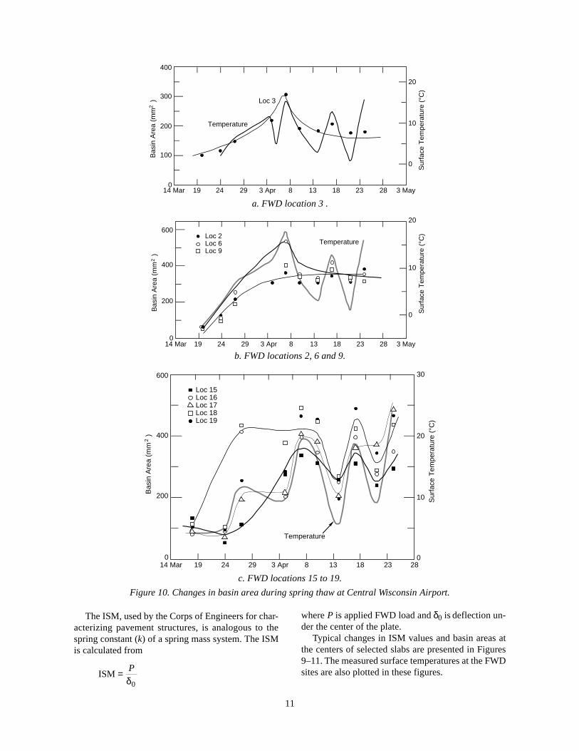
Figure 10. Changes in basin area during spring thaw at Central Wisconsin Airport.
The ISM, used by the Corps of Engineers for char-acterizing pavement structures, is analogous to thespring constant (k) of a spring mass system. The ISMis calculated from
ISM = P
δ0
where P is applied FWD load and δ0 is deflection un-der the center of the plate.
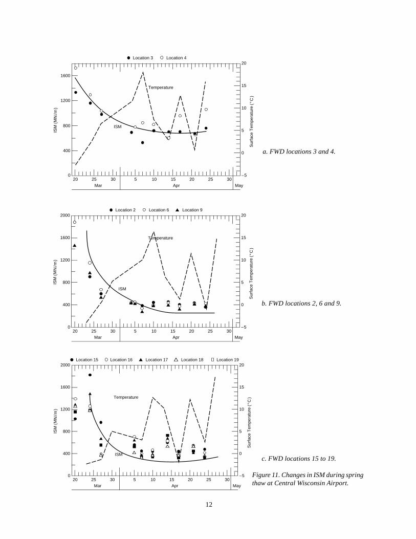
Typical changes in ISM values and basin areas atthe centers of selected slabs are presented in Figures9–11. The measured surface temperatures at the FWDsites are also plotted in these figures.
12
1600
1200
800
400
020 25 30 5 10 15 20 25 30
Mar Apr May
ISM
(M
N/m
)
20
15
10
5
0
–5
Sur
face
Tem
pera
ture
(°C
)
Location 3 Location 4
ISM
Temperature
2000
1600
1200
800
400
020 25 30 5 10 15 20 25 30
Mar Apr May
ISM
(M
N/m
)
20
15
10
5
0
–5
Sur
face
Tem
pera
ture
(°C
)
ISM
Temperature
Location 2 Location 6 Location 9
b. FWD locations 2, 6 and 9.
a. FWD locations 3 and 4.
Figure 11. Changes in ISM during springthaw at Central Wisconsin Airport.
c. FWD locations 15 to 19.
ISM
(M
N/m
)
2000
1600
1200
800
400
020 25 30 5 10 15 20 25 30
Mar Apr May
20
15
10
5
0
–5
Location 15 Location 16 Location 17 Location 18 Location 19
ISM
Sur
face
Tem
pera
ture
(°C
)Temperature
800
600
400
200
Bas
in A
rea
(mm
)
2
Surface Temperature (°C)
Outagamie County Airport
1000
0 10 20 30
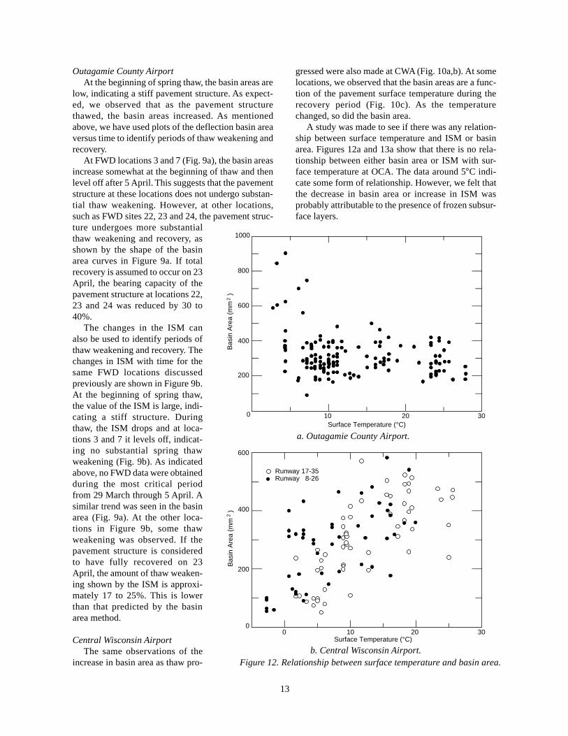
Outagamie County AirportAt the beginning of spring thaw, the basin areas are
low, indicating a stiff pavement structure. As expect-ed, we observed that as the pavement structurethawed, the basin areas increased. As mentionedabove, we have used plots of the deflection basin areaversus time to identify periods of thaw weakening andrecovery.
At FWD locations 3 and 7 (Fig. 9a), the basin areasincrease somewhat at the beginning of thaw and thenlevel off after 5 April. This suggests that the pavementstructure at these locations does not undergo substan-tial thaw weakening. However, at other locations,such as FWD sites 22, 23 and 24, the pavement struc-ture undergoes more substantialthaw weakening and recovery, asshown by the shape of the basinarea curves in Figure 9a. If totalrecovery is assumed to occur on 23April, the bearing capacity of thepavement structure at locations 22,23 and 24 was reduced by 30 to40%.
The changes in the ISM canalso be used to identify periods ofthaw weakening and recovery. Thechanges in ISM with time for thesame FWD locations discussedpreviously are shown in Figure 9b.At the beginning of spring thaw,the value of the ISM is large, indi-cating a stiff structure. Duringthaw, the ISM drops and at loca-tions 3 and 7 it levels off, indicat-ing no substantial spring thawweakening (Fig. 9b). As indicatedabove, no FWD data were obtainedduring the most critical periodfrom 29 March through 5 April. Asimilar trend was seen in the basinarea (Fig. 9a). At the other loca-tions in Figure 9b, some thawweakening was observed. If thepavement structure is consideredto have fully recovered on 23April, the amount of thaw weaken-ing shown by the ISM is approxi-mately 17 to 25%. This is lowerthan that predicted by the basinarea method.
Central Wisconsin AirportThe same observations of the
increase in basin area as thaw pro-
13
gressed were also made at CWA (Fig. 10a,b). At somelocations, we observed that the basin areas are a func-tion of the pavement surface temperature during therecovery period (Fig. 10c). As the temperaturechanged, so did the basin area.
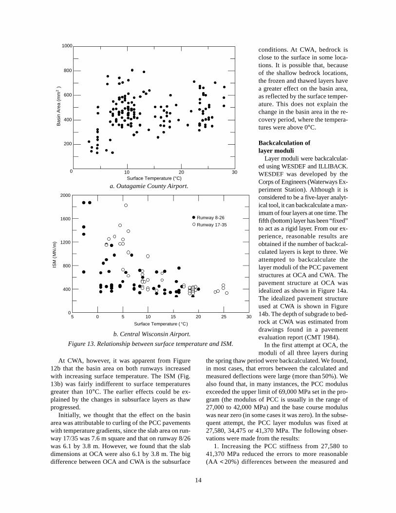
A study was made to see if there was any relation-ship between surface temperature and ISM or basinarea. Figures 12a and 13a show that there is no rela-tionship between either basin area or ISM with sur-face temperature at OCA. The data around 5°C indi-cate some form of relationship. However, we felt thatthe decrease in basin area or increase in ISM wasprobably attributable to the presence of frozen subsur-face layers.
Figure 12. Relationship between surface temperature and basin area.b. Central Wisconsin Airport.
600
400
200
Bas
in A
rea
(mm
)
2
Surface Temperature (°C)
Central Wisconsin Airport
10 20 300
0
Runway 17-35Runway 8-26
a. Outagamie County Airport.
2000
1600
1200
800
400
05 0 105 15 20 25 30
Surface Temperature ( °C )
ISM
( M
N / m
)
Central Wisconcin Airport
Runway 08 - 26
Runway 17 - 35
800
600
400
200
Bas
in A
rea
(mm
)
2
Surface Temperature (°C)
Outagamie County Airport
1000
0 10 20 30
14
At CWA, however, it was apparent from Figure12b that the basin area on both runways increasedwith increasing surface temperature. The ISM (Fig.13b) was fairly indifferent to surface temperaturesgreater than 10°C. The earlier effects could be ex-plained by the changes in subsurface layers as thawprogressed.
Initially, we thought that the effect on the basinarea was attributable to curling of the PCC pavementswith temperature gradients, since the slab area on run-way 17/35 was 7.6 m square and that on runway 8/26was 6.1 by 3.8 m. However, we found that the slabdimensions at OCA were also 6.1 by 3.8 m. The bigdifference between OCA and CWA is the subsurface
conditions. At CWA, bedrock isclose to the surface in some loca-tions. It is possible that, becauseof the shallow bedrock locations,the frozen and thawed layers havea greater effect on the basin area,as reflected by the surface temper-ature. This does not explain thechange in the basin area in the re-covery period, where the tempera-tures were above 0°C.
Backcalculation oflayer moduli Layer moduli were backcalculat-ed using WESDEF and ILLIBACK.WESDEF was developed by theCorps of Engineers (Waterways Ex-periment Station). Although it isconsidered to be a five-layer analyt-ical tool, it can backcalculate a max-imum of four layers at one time. Thefifth (bottom) layer has been “fixed”to act as a rigid layer. From our ex-perience, reasonable results areobtained if the number of backcal-culated layers is kept to three. Weattempted to backcalculate thelayer moduli of the PCC pavementstructures at OCA and CWA. Thepavement structure at OCA wasidealized as shown in Figure 14a.The idealized pavement structureused at CWA is shown in Figure14b. The depth of subgrade to bed-rock at CWA was estimated fromdrawings found in a pavementevaluation report (CMT 1984). In the first attempt at OCA, themoduli of all three layers during
the spring thaw period were backcalculated. We found,in most cases, that errors between the calculated andmeasured deflections were large (more than 50%). Wealso found that, in many instances, the PCC modulusexceeded the upper limit of 69,000 MPa set in the pro-gram (the modulus of PCC is usually in the range of27,000 to 42,000 MPa) and the base course moduluswas near zero (in some cases it was zero). In the subse-quent attempt, the PCC layer modulus was fixed at27,580, 34,475 or 41,370 MPa. The following obser-vations were made from the results:
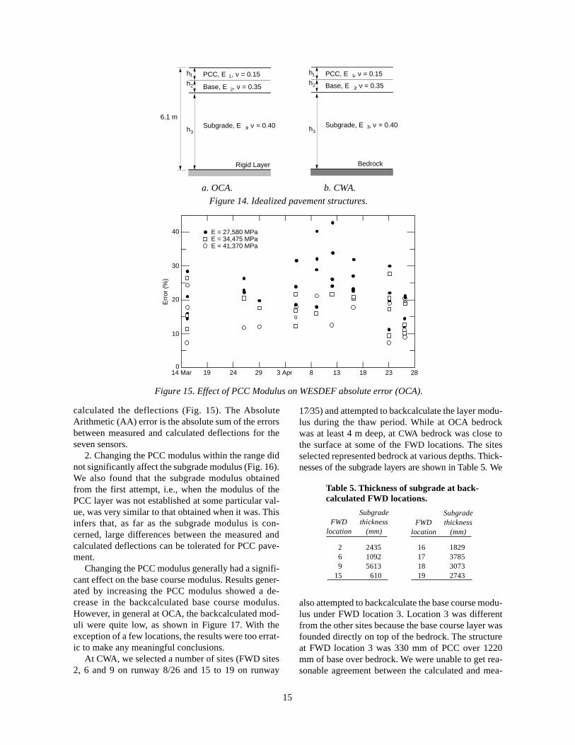
1. Increasing the PCC stiffness from 27,580 to41,370 MPa reduced the errors to more reasonable(AA < 20%) differences between the measured and
Figure 13. Relationship between surface temperature and ISM.
b. Central Wisconsin Airport.
a. Outagamie County Airport.
Runway 8-26
Runway 17-35
15
calculated the deflections (Fig. 15). The AbsoluteArithmetic (AA) error is the absolute sum of the errorsbetween measured and calculated deflections for theseven sensors.
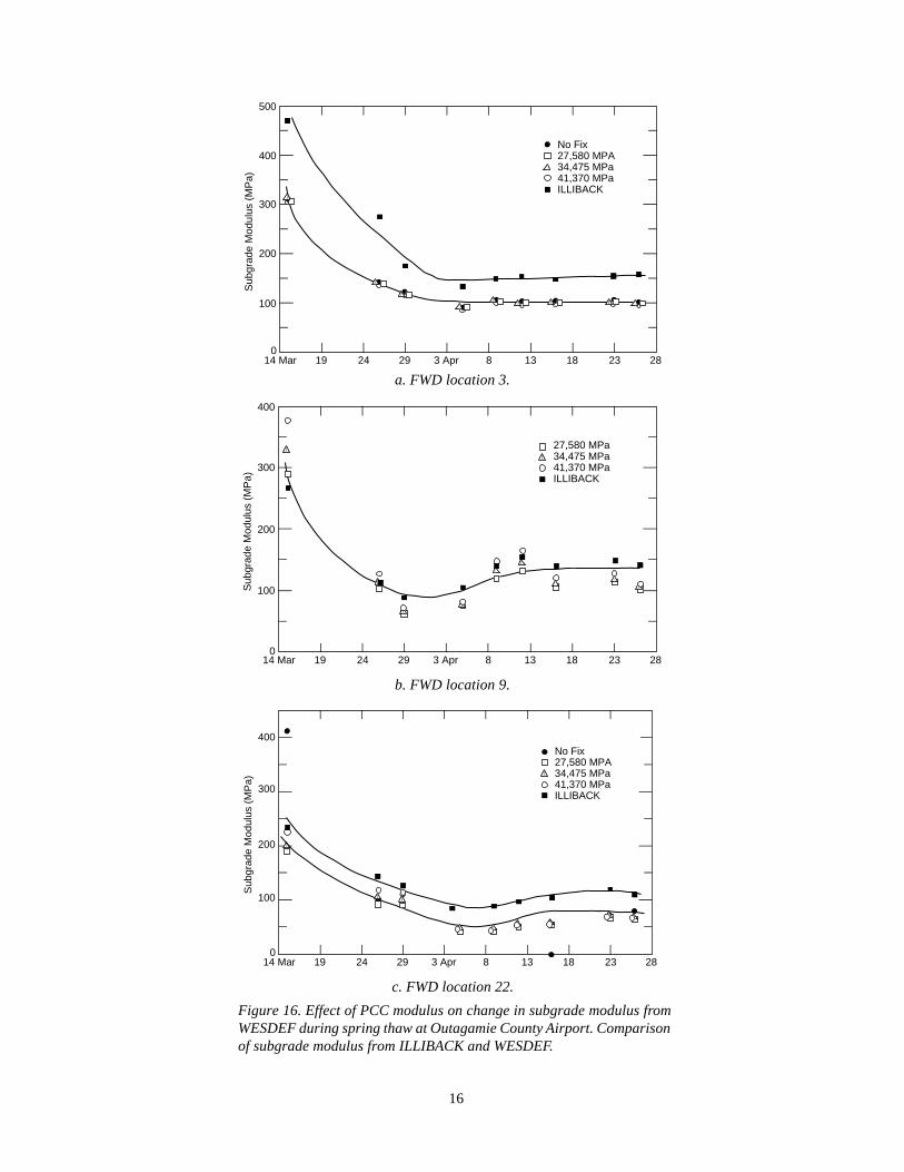
2. Changing the PCC modulus within the range didnot significantly affect the subgrade modulus (Fig. 16).We also found that the subgrade modulus obtainedfrom the first attempt, i.e., when the modulus of thePCC layer was not established at some particular val-ue, was very similar to that obtained when it was. Thisinfers that, as far as the subgrade modulus is con-cerned, large differences between the measured andcalculated deflections can be tolerated for PCC pave-ment.
Changing the PCC modulus generally had a signifi-cant effect on the base course modulus. Results gener-ated by increasing the PCC modulus showed a de-crease in the backcalculated base course modulus.However, in general at OCA, the backcalculated mod-uli were quite low, as shown in Figure 17. With theexception of a few locations, the results were too errat-ic to make any meaningful conclusions.
At CWA, we selected a number of sites (FWD sites2, 6 and 9 on runway 8/26 and 15 to 19 on runway
17⁄35) and attempted to backcalculate the layer modu-lus during the thaw period. While at OCA bedrockwas at least 4 m deep, at CWA bedrock was close tothe surface at some of the FWD locations. The sitesselected represented bedrock at various depths. Thick-nesses of the subgrade layers are shown in Table 5. We
also attempted to backcalculate the base course modu-lus under FWD location 3. Location 3 was differentfrom the other sites because the base course layer wasfounded directly on top of the bedrock. The structureat FWD location 3 was 330 mm of PCC over 1220mm of base over bedrock. We were unable to get rea-sonable agreement between the calculated and mea-
6.1 m
h1
Rigid Layer
PCC, E , ν = 0.151
Subgrade, E , ν = 0.403
2h
3h
Base, E , ν = 0.352
a. OCA. b. CWA.
h1
Bedrock
2h
3h
PCC, E , ν = 0.151
Subgrade, E , ν = 0.403
Base, E , ν = 0.352
Figure 14. Idealized pavement structures.
30
40
20
10
014 Mar 19 24 29 3 Apr 13 188 23 28
Err
or (
%)
Outagamie County Airport
E = 27,580 MPaE = 34,475 MPaE = 41,370 MPa
Figure 15. Effect of PCC Modulus on WESDEF absolute error (OCA).
SubgradeFWD thickness
location (mm)
2 24356 10929 5613
15 610
16 182917 378518 307319 2743
SubgradeFWD thickness
location (mm)
Table 5. Thickness of subgrade at back-calculated FWD locations.
16
a. FWD location 3.
b. FWD location 9.
c. FWD location 22.
Figure 16. Effect of PCC modulus on change in subgrade modulus fromWESDEF during spring thaw at Outagamie County Airport. Comparisonof subgrade modulus from ILLIBACK and WESDEF.
400
300
200
014 Mar 19 24 29 3 Apr 13 188 23 28
Sub
grad
e M
odul
us (
MP
a)
Outagamie County Airport
100
No Fix27,580 MPA34,475 MPa41,370 MPaILLIBACK
400
500
300
200
014 Mar 19 24 29 3 Apr 13 188 23 28
Sub
grad
e M
odul
us (
MP
a)
Outagamie County Airport
100
No Fix27,580 MPA34,475 MPa41,370 MPaILLIBACK
400
300
200
014 Mar 19 24 29 3 Apr 13 188 23 28
Sub
grad
e M
odul
us (
MP
a)
Outagamie County Airport
100
27,580 MPa34,475 MPa41,370 MPaILLIBACK

FWD PCC Base Subgrade AA ErrorDate location (MPa) (MPa) (MPa) (%)
20 Mar 2 27,580 54,148 433 —24 Mar 2 27,580 6,807 214 26.727 Mar 2 27,580 5,096 97 12.04 Apr 2 27,580 2,123 70 12.37 Apr 2 27,580 1,832 56 17.110 Apr 2 27,580 2,002 70 16.014 Apr 2 27,580 2,791 65 21.417 Apr 2 27,580 2,284 56 16.921 Apr 2 27,580 4,087 56 15.024 Apr 2 27,580 2,402 47 16.320 Mar 9 27,580 4,965 825 13.324 Mar 9 27,580 1,935 455 17.427 Mar 9 27,580 1,373 162 20.64 Apr 9 27,580 643 139 14.57 Apr 9 27,580 526 62 14.410 Apr 9 27,580 1,050 107 16.914 Apr 9 27,580 1,495 111 9.517 Apr 9 27,580 1,200 81 13.821 Apr 9 27,580 1,547 116 16.924 Apr 9 27,580 1,612 99 18.318 Mar 17 27,580 5,956 425 31.624 Mar 17 27,580 4,802 589 12.827 Mar 17 27,580 2,071 157 11.64 Apr 17 27,580 2,821 131 5.97 Apr 17 27,580 1,747 51 10.9
17
8000
6000
4000
014 Mar 19 24 29 3 Apr 13 188 23 28
Bas
e C
ours
e M
odul
us (
MP
a)
Outagamie County Airport
2000
Loc 3Loc 9Loc 22Loc 23
Figure 17. Backcalculated base course modulus using WESDEF (OCA).
10 Apr 17 27,580 1,520 58 8.414 Apr 17 27,580 3,717 133 3.917 Apr 17 27,580 2,416 57 8.721 Apr 17 27,580 3,560 50 8.924 Apr 17 27,580 18,212 18 129.218 Mar 18 27,580 149 595 —24 Mar 18 27,580 3,216 367 23.027 Mar 18 27,580 3,645 32 10.84 Apr 18 27,580 4,027 39 9.67 Apr 18 27,580 3,499 26 4.610 Apr 18 27,580 4,713 29 9.114 Apr 18 27,580 2,611 82 5.217 Apr 18 27,580 2,035 39 7.021 Apr 18 27,580 — — —24 Apr 18 27,580 2,572 35 8.918 Mar 19 27,580 5,648 272 11.424 Mar 19 27,580 5,133 316 —27 Mar 19 27,580 — — —4 Apr 19 27,580 — — —7 Apr 19 27,580 2,163 29 8.210 Apr 19 27,580 1,852 32 7.014 Apr 19 27,580 — — —17 Apr 19 27,580 1,482 29 9.321 Apr 19 27,580 — — —24 Apr 19 27,580 1,891 30 8.8
FWD PCC Base Subgrade AA ErrorDate location (MPa) (MPa) (MPa) (%)
Table 6. Backcalculated modulus at CWA using WESDEF.
lack of values in the base modulus, subgrade modulusand error columns in Table 6 indicate that either it wasnot possible to converge to a solution or that the basecourse modulus was extremely low (less than 1 MPa).When only the AA error column lacks values, itmeans that we used the backcalculated results fromWESDEF but ignored the controlling layer modulusrange, i.e., the backcalculated modulus was eitherabove or below the prescribed range.
The effect of changing the PCC modulus is shownin Table 7 for FWD locations 9, 17, 18 and 19. As
sured deflections. The AA error was in the vicinity of450%.
Solutions could not be obtained for locations 6, 15and 16. In many cases, WESDEF printed a “THISMATRIX HAS NO SOLUTION” message. At othertimes, the backcalculated base course modulus waszero, or very close to zero. It is interesting to note thatat these locations the bedrock was quite close to thesurface (less than 2 m). At the other locations, with afew exceptional days, the error between the calculatedand measured values was acceptable (Table 6). The
18
Table 7. Effect of change in PCC modulus on base and subgrade modulus.
FWD PCC Base Subgrade AA error PCC Base Subgrade AA errorDate location (MPa) (MPa) (MPa) (%) (MPa) (MPa) (MPa) (%)
20 Mar 9 27,580 4,965 825 13.3 34,475 3617 828 12.324 Mar 9 27,580 1,935 455 17.4 34,475 1045 463 12.827 Mar 9 27,580 1,373 162 20.6 34,475 529 165 17.74 Apr 9 27,580 643 139 14.5 34,475 81 155 10.37 Apr 9 27,580 526 62 14.4 34,475 16 81 11.510 Apr 9 27,580 1,050 107 16.9 34,475 255 110 14.314 Apr 9 27,580 1,495 111 9.5 34,475 537 113 8.917 Apr 9 27,580 1,200 81 13.8 34,475 387 82 11.721 Apr 9 27,580 1,547 116 16.9 34,475 685 118 15.124 Apr 9 27,580 1,612 99 18.3 34,475 749 100 16.218 Mar 17 27,580 5,956 425 31.6 34,475 4092 429 32.224 Mar 17 27,580 4,802 589 12.8 34,475 3038 595 9.727 Mar 17 27,580 2,071 157 11.6 34,475 — — —4 Apr 17 27,580 2,821 131 5.9 34,475 1455 134 5.87 Apr 17 27,580 1,747 51 10.9 34,475 639 52 9.410 Apr 17 27,580 1,520 58 8.4 34,475 316 59 8.314 Apr 17 27,580 3,717 133 3.9 34,475 2282 135 4.217 Apr 17 27,580 2,416 57 8.7 34,475 — — —21 Apr 17 27,580 3,560 50 8.9 34,475 2350 49 7.824 Apr 17 27,580 18,212 18 129.2 34,475 — — —18 Mar 18 27,580 149 595 — 34,475 — — —24 Mar 18 27,580 3,216 367 23.0 34,475 1750 373 19.427 Mar 18 27,580 3,645 32 10.8 34,475 2335 33 9.24 Apr 18 27,580 4,027 39 9.6 34,475 — — —7 Apr 18 27,580 3,499 26 4.6 34,475 2241 26 3.510 Apr 18 27,580 4,713 29 9.1 34,475 2609 30 2.114 Apr 18 27,580 2,611 82 5.2 34,475 — — —17 Apr 18 27,580 2,035 39 7.0 34,475 708 40 7.221 Apr 18 27,580 — — — 34,475 — — —24 Apr 18 27,580 2,572 35 8.9 34,475 1473 36 9.718 Mar 19 27,580 5,648 272 11.4 34,475 3839 278 8.624 Mar 19 27,580 5,133 316 — 34,475 3195 319 11.527 Mar 19 27,580 — — — 34,475 — — —4 Apr 19 27,580 — — — 34,475 — — —7 Apr 19 27,580 2,163 29 8.2 34,475 830 30 8.010 Apr 19 27,580 1,852 32 7.0 34,475 551 33 7.414 Apr 19 27,580 — — — 34,475 — — —17 Apr 19 27,580 1,482 29 9.3 34,475 444 30 8.221 Apr 19 27,580 — — — 34,475 — — —24 Apr 19 27,580 1,891 30 8.8 34,475 591 31 8.3
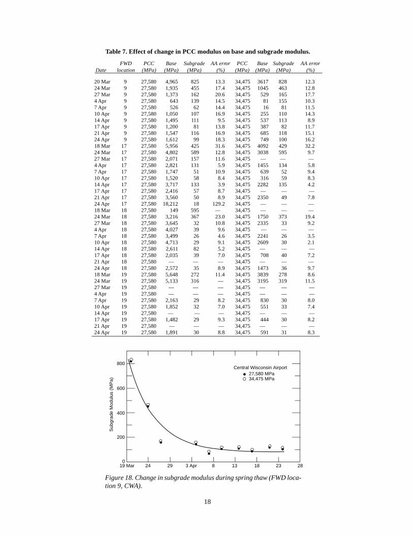
Figure 18. Change in subgrade modulus during spring thaw (FWD loca-tion 9, CWA).
800
600
400
200
019 Mar 24 29 3 Apr 8 13 18 23 28
Central Wisconsin Airport27,580 MPa34,475 MPa
Sub
grad
e M
odul
us (
MP
a)
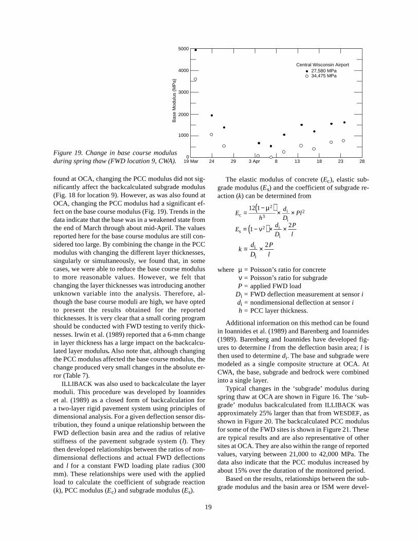
found at OCA, changing the PCC modulus did not sig-nificantly affect the backcalculated subgrade modulus(Fig. 18 for location 9). However, as was also found atOCA, changing the PCC modulus had a significant ef-fect on the base course modulus (Fig. 19). Trends in thedata indicate that the base was in a weakened state fromthe end of March through about mid-April. The valuesreported here for the base course modulus are still con-sidered too large. By combining the change in the PCCmodulus with changing the different layer thicknesses,singularly or simultaneously, we found that, in somecases, we were able to reduce the base course modulusto more reasonable values. However, we felt thatchanging the layer thicknesses was introducing anotherunknown variable into the analysis. Therefore, al-though the base course moduli are high, we have optedto present the results obtained for the reportedthicknesses. It is very clear that a small coring programshould be conducted with FWD testing to verify thick-nesses. Irwin et al. (1989) reported that a 6-mm changein layer thickness has a large impact on the backcalcu-lated layer modulus. Also note that, although changingthe PCC modulus affected the base course modulus, thechange produced very small changes in the absolute er-ror (Table 7).
ILLIBACK was also used to backcalculate the layermoduli. This procedure was developed by Ioannideset al. (1989) as a closed form of backcalculation fora two-layer rigid pavement system using principles ofdimensional analysis. For a given deflection sensor dis-tribution, they found a unique relationship between theFWD deflection basin area and the radius of relativestiffness of the pavement subgrade system (l). Theythen developed relationships between the ratios of non-dimensional deflections and actual FWD deflectionsand l for a constant FWD loading plate radius (300mm). These relationships were used with the appliedload to calculate the coefficient of subgrade reaction(k), PCC modulus (Ec) and subgrade modulus (Es).
19
The elastic modulus of concrete (Ec), elastic sub-grade modulus (Es) and the coefficient of subgrade re-action (k) can be determined from
Eh
d
DPlc
i
i=
−( )× ×
12 1 2
32
µ
Ed
D
P
lsi
i= −( ) × ×1
22ν
kd
D
P
l= ×i
i
2
where µ = Poisson’s ratio for concreteν = Poisson’s ratio for subgrade
P = applied FWD loadDi = FWD deflection measurement at sensor i di = nondimensional deflection at sensor ih = PCC layer thickness.
Additional information on this method can be foundin Ioannides et al. (1989) and Barenberg and Ioannides(1989). Barenberg and Ioannides have developed fig-ures to determine l from the deflection basin area; l isthen used to determine di . The base and subgrade weremodeled as a single composite structure at OCA. AtCWA, the base, subgrade and bedrock were combinedinto a single layer.
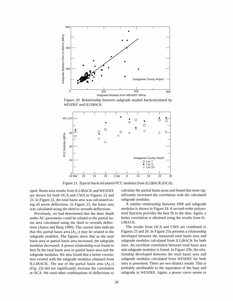
Typical changes in the ‘subgrade’ modulus duringspring thaw at OCA are shown in Figure 16. The ‘sub-grade’ modulus backcalculated from ILLIBACK wasapproximately 25% larger than that from WESDEF, asshown in Figure 20. The backcalculated PCC modulusfor some of the FWD sites is shown in Figure 21. Theseare typical results and are also representative of othersites at OCA. They are also within the range of reportedvalues, varying between 21,000 to 42,000 MPa. Thedata also indicate that the PCC modulus increased byabout 15% over the duration of the monitored period.
Based on the results, relationships between the sub-grade modulus and the basin area or ISM were devel-
5000
4000
3000
2000
019 Mar 24 29 3 Apr 8 13 18 23 28
Central Wisconsin Airport27,580 MPa34,475 MPa
Bas
e M
odul
us (
MP
a)
1000
Figure 19. Change in base course modulusduring spring thaw (FWD location 9, CWA).
20
600
400
200
0
Subgrade Modulus from WESDEF (MPa)
Sub
grad
e M
odul
us fr
om IL
LIB
AC
K (
MP
a)
600400200
Outagamie County AirportR = 0.82
014 Mar 19 24 29 3 Apr 8 18 23 28
PC
C M
odul
us (
MP
a)
Outagamie County AirportLoc 7Loc 9Loc 23
40 x 103
30
20
10
13
Figure 20. Relationship between subgrade moduli backcalculated byWESDEF and ILLIBACK.
Figure 21. Typical backcalculated PCC modulus from ILLIBACK (OCA).
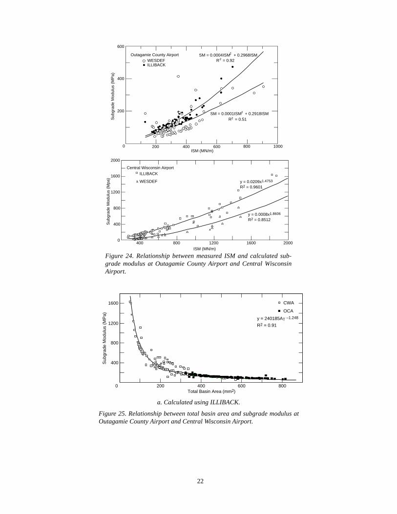
oped. Basin area results from ILLIBACK and WESDEFare shown for both OCA and CWA in Figures 22 and23. In Figure 22, the total basin area was calculated us-ing all seven deflections. In Figure 23, the basin areawas calculated using the third to seventh deflections.
Previously, we had determined that the thaw depthunder AC pavements could be related to the partial ba-sin area calculated using the third to seventh deflec-tions (Janoo and Berg 1990). The current data indicatethat this partial basin area (A3-7) may be related to thesubgrade modulus. The figures show that as the totalbasin area or partial basin area increased, the subgrademodulus decreased. A power relationship was found tobest fit the total basin area or partial basin area and thesubgrade modulus. We also found that a better correla-tion existed with the subgrade modulus obtained fromILLIBACK. The use of the partial basin area (A3-7)(Fig. 23) did not significantly increase the correlationat OCA. We used other combinations of deflections to
calculate the partial basin areas and found that none sig-nificantly increased the correlation with the calculatedsubgrade modulus.
A similar relationship between ISM and subgrademodulus is shown in Figure 24. A second-order polyno-mial function provides the best fit to the data. Again, abetter correlation is obtained using the results from IL-LIBACK .
The results from OCA and CWA are combined inFigures 25 and 26. In Figure 25a presents a relationshipdeveloped between the measured total basin area andsubgrade modulus calculated from ILLIBACK for bothsites. An excellent correlation between total basin areaand subgrade modulus is found. In Figure 25b, the rela-tionship developed between the total basin area andsubgrade modulus calculated from WESDEF for bothsites is presented. There are two distinct trends. This isprobably attributable to the separation of the base andsubgrade in WESDEF. Again, a power curve seems to

21
0
Sub
grad
e M
odul
us (
MP
a)
Outagamie County AirportWESDEFILLIBACK
200 400 600 Basin Area (mm )2
600
400
200
R = 0.972
– 1.1175SM = 86156A 3-7
R = 0.652SM = 35778A
– 1.00963-7
Figure 23. Relationship between measuredpartial basin area (third–seventh deflec-tions) and calculated subgrade modulus atOutagamie County Airport.
Figure 22. Relationship between measured total basin area and cal-culated subgrade modulus.
600
400
200
0 200 400 600 800
Total Basin Area ( mm 2
)
Sub
grad
e M
odul
us (
MP
a )
Outagamie County Airport
ILLIBACK
WESDEF
y = 43006x –0.9954
R 2 = 0.60
y = 134316x –
1.1412
R 2 = 0.96
1600
1200
800
0
Sub
grad
e M
odul
us (
MP
a)
600400200
Outagamie County AirportWESDEFILLIBACK
Total Basin Area (mm )2
400
y = 154319x – 1.1708
R = 0.992
y = 116238x – 1.3034
R = 0.702
Central Wisconsin Airport
22
0
Sub
grad
e M
odul
us (
MP
a)
Outagamie County AirportWESDEFILLIBACK
200 400 600ISM (MN/m)
600
400
200
800 1000
SM = 0.0004ISM + 0.2968ISM2
R = 0.922
SM = 0.0001ISM + 0.2918ISM2
R = 0.512
ILLIBACK
WESDEF
ISM (MN/m)
Sub
grad
e M
odul
us (
Mpa
)
0
400
800
1200
1600
2000
400 800 1200 1600 2000
y = 0.0209x1.4753
R2 = 0.9601
y = 0.0008x1.8606
R2 = 0.8512
Central Wisconsin Airport
Figure 24. Relationship between measured ISM and calculated sub-grade modulus at Outagamie County Airport and Central WisconsinAirport.
a. Calculated using ILLIBACK.
Figure 25. Relationship between total basin area and subgrade modulus atOutagamie County Airport and Central Wisconsin Airport.
CWA
OCA
Total Basin Area (mm2)
Sub
grad
e M
odul
us (
MP
a)
400
800
1200
1600
0 200 400 600 800
y = 240185AT –1.248
R2 = 0.91

23
b. Calculated using WESDEF.
c. Calculated using WESDEF with a single power trend.
Figure 25 (cont’d).
Total Basin Area (mm2)
Coe
ffici
ent o
f Sub
grad
e R
eact
ion
(MN
/m3)
400
800
1200
0 200 400 600 800
CWA
OCA
y = 741480x–1.6662
R2 = 0.86
Figure 26. Relationship between total basin area and coefficient of subgradereaction calculated using ILLIBACK at Outagamie County Airport and Cen-tral Wisconsin Airport.
0
Sub
grad
e M
odul
us (
MP
a)
200 400 600
200
800
400
1000
Total Basin Area (mm )2
WESDEF
R = 0.702y = 116238x– 1.3034
y = 43006x– 0.9954
R = 0.592
600
OCACWA
800
0
Sub
grad
e M
odul
us (
MP
a)
200 400 600
200
800
400
1000
Total Basin Area (mm )2
WESDEF
y = 10773x– 1.796
600
OCACWA
800
R = 0.912

24
Table 9. Gear information for computer simulations of theMD-DC9 and Boeing 757.
Contact Contact Load onAircraft Tire Radius area pressure tire X-cord Y-cord
type no. (mm) (m2) (kPa) (kN) (mm) (mm)
MD-DC9 1 181.4 0.103 1103 114.1 –330.2 02 181.4 0.103 1103 114.1 330.2 0
Boeing 757 1 189.5 0.113 1172 132.1 –431.8 02 189.5 0.113 1172 132.1 431.8 03 189.5 0.113 1172 132.1 –431.8 11434 189.5 0.113 1172 132.1 431.8 1143
best fit the data, so for estimation, a single powertrend was applied to the data as shown in Figure 25c.Figure 26 shows the relationship between the meas-ured total basin area and the coefficient of subgradereaction (k) computed from ILLIBACK for both sitesThe following equations have been developed fromthe ILLIBACK results and can be used to estimate thesubgrade modulus and the coefficient of subgrade re-action (k)
SM A= 240 185, T–1.248 (R2 = 0.91)
k A= 741 480, T–1.6662 (R2 = 0.86)
whereSM = subgrade modulus (MPa)AT = total basin area (mm2)k = coefficient of subgrade reaction
(MN/m3).
2000
1600
1200
400
0 400 800 1200 1600 2000ISM (MN/m)
Sub
grad
e M
odul
us (
MP
a)
800
WESDEFILLIBACK
OCA
WESDEFILLIBACK
CWA
2y = 0.0004 ISM + 0.1378 ISM + 41.57R = 0.962
y = 0.0003 ISM – 0.0365 ISM + 72.572
R = 0.732
Figure 27. Relationship between ISM andsubgrade modulus at OCA and CWA.
Table 8. Gear loading for the MD-DC9 and Boeing 757.
Aircraft Design load % of design load Load on main gear type (MN) on each main gear (MN)
MD-DC9 480 47.5 228.2Boeing 757 1112 47.5 528.2
In Figure 27, the relationship of ISM and subgrademodulus for both OCA and CWA is shown. Again, asingle power curve can be fitted to the data.
Current criteria for PCC pavements state that failureoccurs when the horizontal tensile stress at the bottomof the PCC layer is equal to or greater than the flexuralstrength of the slab. The flexural strength reported atOCA and CWA was 4.5 MPa. The two types of aircraftused for these simulations were the MD-DC9 and theBoeing 757. The gear loads, tire spacings and radiiwere obtained from the FAALEA computer programand are presented in Tables 8 and 9.
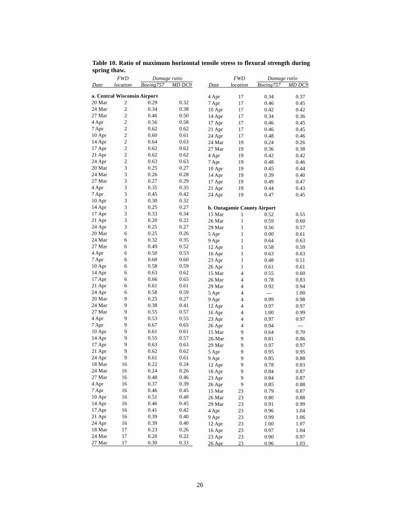
Several FWD locations were selected from each air-port for computing the tensile stress at the bottom of thePCC layer on different days during the monitoring peri-od. The damage (D) reported here is defined as the ratioof maximum horizontal (tensile) stress to the flexural

25
r = 1814mm
3
2 1
4
86.8mm
228.6mm
330.2mm
330.2mm
b. MD: DC 9
13
4
3 2 1
r = 189.5mm
1143mm254
mm
101.6mm 218.9
mm
431.8mm
431.8mm
a. Boeing 757
Figure 28. Configuration and location of stress calculations for Boeing 757 and MD-DC9.
80
60
40
20
0
D, D
amag
e (%
)
100
14 Mar 19 24 29 3 Apr 8 13 18 23 28
LOC 2LOC 3LOC 6LOC 9LOC 16LOC 17LOC 19LOC 24
Boeing 757Central Wisconsin Airport
254 mm
305
330
Figure 29. Amount of damage during spring thaw at Central Wis-consin Airport.
Figure 30. Effect of pavement thickness on damage at CentralWisconsin Airport.
strength of the PCC layer
D = σσ
tensile
flexural.
Layer moduli from ILLIBACK were usedto represent the pavement structures. Thecomputer program BISAR was used to calcu-late the stresses at locations shown in Figure28. The stress calculation points are the sameas those used in FAALEA. The results aretabulated in Table 10 and damage is shownfor CWA in Figure 29. As thaw progresses,the amount of damage increases until thaw-ing is complete; then it levels off with time.The results also indicate that the damage is afunction of pavement thickness, a linear rela-tionship being found in the 24 April datafrom CWA (Fig. 30).
The thinner pavements (178 to 203 mm)at OCA showed potential near-failure condi-tions during the spring thaw (Fig. 31). Somepavements recovered somewhat, as typifiedby location 9 (Fig. 31). The thicker section(location 23, 254 mm) had a similar amountof damage as those sections of similar thick-ness at CWA; however, the OCA sections didnot exhibit the loss during the thawing peri-od observed at CWA.
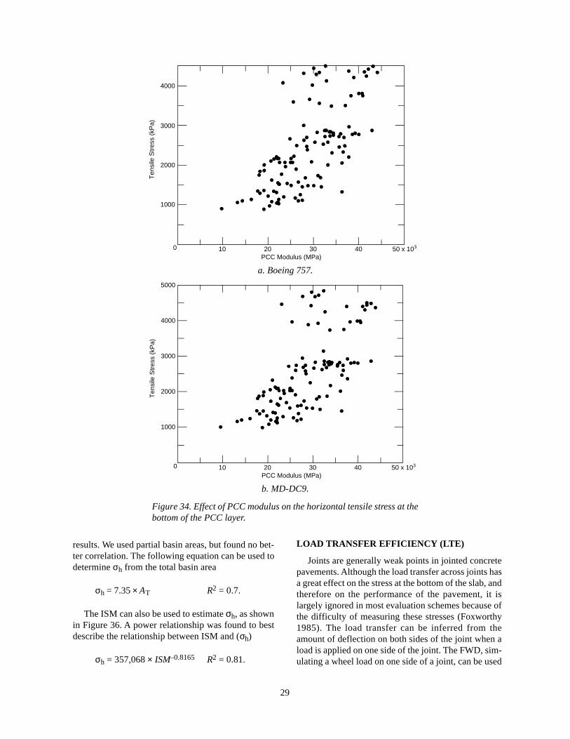
The horizontal stresses are plotted asfunctions of the subgrade modulus, coeffi-cient of subgrade reaction and the PCC mod-ulus in Figures 32–34. With respect to thePCC modulus, no trends were seen (Fig. 34),and nonlinear trends were observed for all of
0.8
0.6
0.4
0
Dam
age
1.0
0.2
200 220 240 260 280 300 320 340PCC Thickness (mm)
D = – 0.004t + 1.6356R = 0.952
FWD Damage ratioDate location Boeing757 MD DC9
a. Central Wisconsin Airport20 Mar 2 0.29 0.3224 Mar 2 0.34 0.3827 Mar 2 0.46 0.504 Apr 2 0.56 0.587 Apr 2 0.62 0.6210 Apr 2 0.60 0.6114 Apr 2 0.64 0.6317 Apr 2 0.62 0.6221 Apr 2 0.62 0.6224 Apr 2 0.63 0.6320 Mar 3 0.25 0.2724 Mar 3 0.26 0.2827 Mar 3 0.27 0.294 Apr 3 0.35 0.357 Apr 3 0.45 0.4210 Apr 3 0.30 0.3214 Apr 3 0.25 0.2717 Apr 3 0.33 0.3421 Apr 3 0.20 0.2224 Apr 3 0.25 0.2720 Mar 6 0.25 0.2624 Mar 6 0.32 0.3527 Mar 6 0.49 0.524 Apr 6 0.50 0.537 Apr 6 0.60 0.6010 Apr 6 0.58 0.5914 Apr 6 0.63 0.6217 Apr 6 0.66 0.6521 Apr 6 0.61 0.6124 Apr 6 0.58 0.5920 Mar 9 0.25 0.2724 Mar 9 0.38 0.4127 Mar 9 0.55 0.574 Apr 9 0.53 0.557 Apr 9 0.67 0.6510 Apr 9 0.61 0.6114 Apr 9 0.55 0.5717 Apr 9 0.63 0.6321 Apr 9 0.62 0.6224 Apr 9 0.61 0.6118 Mar 16 0.22 0.2424 Mar 16 0.24 0.2627 Mar 16 0.48 0.464 Apr 16 0.37 0.397 Apr 16 0.46 0.4510 Apr 16 0.51 0.4814 Apr 16 0.46 0.4517 Apr 16 0.41 0.4221 Apr 16 0.39 0.4024 Apr 16 0.39 0.4018 Mar 17 0.23 0.2624 Mar 17 0.20 0.2227 Mar 17 0.30 0.33
4 Apr 17 0.34 0.377 Apr 17 0.46 0.4510 Apr 17 0.42 0.4214 Apr 17 0.34 0.3617 Apr 17 0.46 0.4521 Apr 17 0.46 0.4524 Apr 17 0.48 0.4624 Mar 19 0.24 0.2627 Mar 19 0.36 0.384 Apr 19 0.42 0.427 Apr 19 0.48 0.4610 Apr 19 0.45 0.4414 Apr 19 0.39 0.4017 Apr 19 0.49 0.4721 Apr 19 0.44 0.4324 Apr 19 0.47 0.45
b. Outagamie County Airport15 Mar 1 0.52 0.5526 Mar 1 0.59 0.6029 Mar 1 0.56 0.575 Apr 1 0.00 0.619 Apr 1 0.64 0.6312 Apr 1 0.58 0.5916 Apr 1 0.63 0.6323 Apr 1 0.48 0.5126 Apr 1 0.61 0.6115 Mar 4 0.55 0.6026 Mar 4 0.78 0.8329 Mar 4 0.92 0.945 Apr 4 — 1.009 Apr 4 0.99 0.9812 Apr 4 0.97 0.9716 Apr 4 1.00 0.9923 Apr 4 0.97 0.9726 Apr 4 0.94 —15 Mar 9 0.64 0.7026-Mar 9 0.81 0.8629 Mar 9 0.97 0.975 Apr 9 0.95 0.959 Apr 9 0.85 0.8812 Apr 9 0.78 0.8316 Apr 9 0.84 0.8723 Apr 9 0.84 0.8726 Apr 9 0.85 0.8815 Mar 23 0.79 0.8726 Mar 23 0.80 0.8829 Mar 23 0.91 0.994 Apr 23 0.96 1.049 Apr 23 0.99 1.0612 Apr 23 1.00 1.0716 Apr 23 0.97 1.0423 Apr 23 0.90 0.9726 Apr 23 0.96 1.03
FWD Damage ratioDate location Boeing757 MD DC9
Table 10. Ratio of maximum horizontal tensile stress to flexural strength duringspring thaw.
26

27
a. Boeing 757.
b. MD-DC9.
Figure 32. Effect of subgrade modulus on the horizontal tensilestress at the bottom of the PCC layer (OCA and CWA).
0.8
0.4
0
Dam
age
1.2
14 Mar 19 24 29 3 Apr 8 13 18 23 28
Boeing 757Outagamie County Airport
LOC 1LOC 4LOC 9LOC 23
178, 203 mm
203
254
Figure 31. Amount of damage during spring thaw at OutagamieCounty Airport.
5000
4000
3000
2000
0 400 800 1200 1600
Ten
sile
Str
ess
(kP
a)
Subgrade Modulus (MPa)
1000
Boeing 757
y = 41732x – 0.5493
R = 0.692
Ten
sile
Str
ess
( kP
a )
Subgrade Modulus ( MPa )
5000
4000
3000
2000
1000
0 400 800 1200 1600
Boeing 757
y = 41732x –
0.5493
R 2 = 0.69

28
Ten
sile
Str
ess
( kP
a )
Subgrade Modulus ( MPa )
5000
4000
3000
2000
1000
0 400 800 1200 1600
Boeing 757
y = 41732x –
0.5493
R 2 = 0.69
a. Boeing 757.
b. MD-DC9.
Figure 33. Effect of the coefficient of subgrade reaction, k, on the horizontaltensile stress at the bottom of the PCC layer.
Since we found damage to be a function of thickness, σhwas developed as a function of Es or k and the coeffi-cient of thickness. We found that the correlations in-creased when thickness was taken into consideration.
σh= 7360 – 1.5Es – 17t
or
σh= 7389 – 13.02k – 17.5t
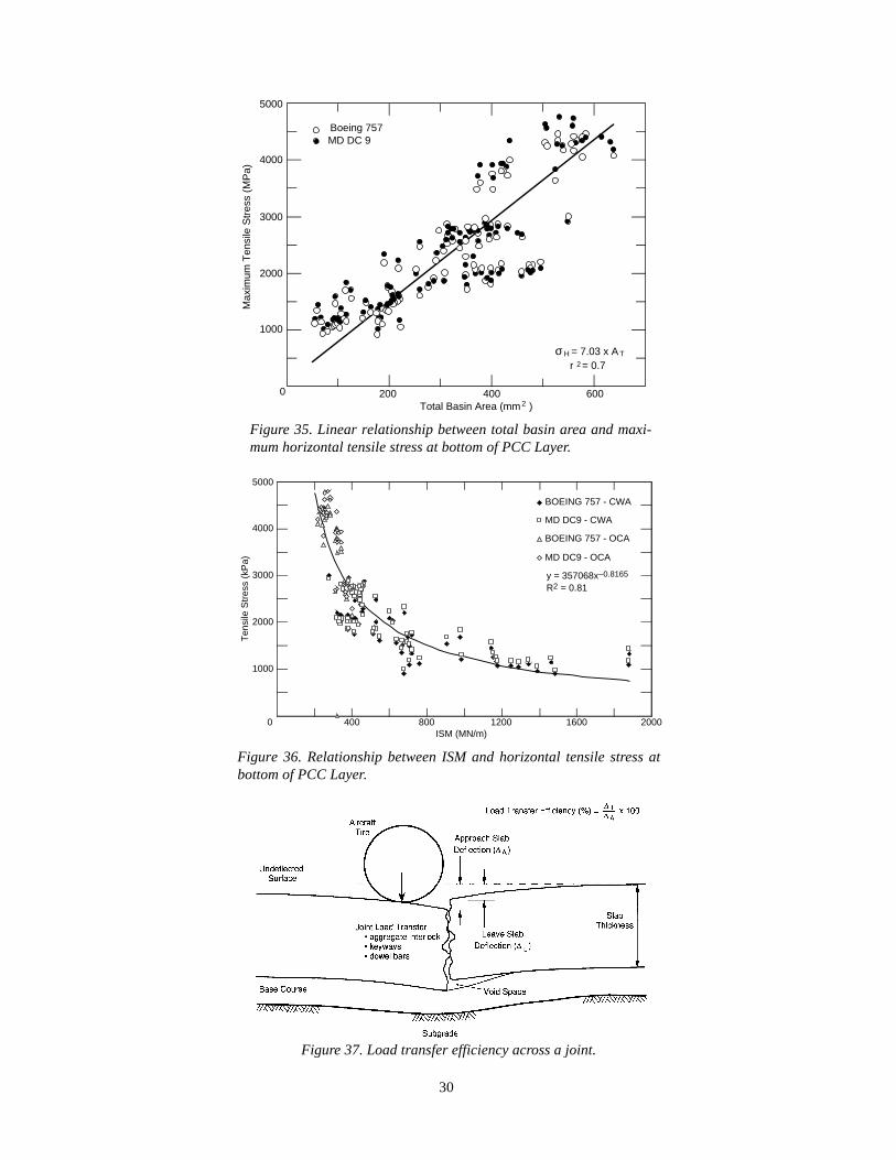
where t is PCC thickness (mm).The relationship between the total basin area and the
horizontal stresses (σh) at the bottom of the PCC layer isshown in Figure 35. A linear trend was applied to the
the other relationships. Small differences were obtainedfor the Boeing 757 and the MD-DC9.
The following equation could be used to estimate thehorizontal stress σh as a function of the subgrade modu-lus Es (MPa) during the spring thaw
σh s–0.549= 41 732, .E
We observed a similar trend between the horizontalstrain and the coefficient of subgrade reaction. The fol-lowing equation could be used to estimate the horizontalstress (σh) as a function of the coefficient of subgradereaction, k (MN/m3) during the spring thaw
σh–0.411= 12 436, .k
5000
4000
2000
0 200 400 600 800
Ten
sile
Str
ess
(kP
a)
MD DC 9y = 10973x– 0.3744
R = 0.542
k, Coefficient of Subgrade Reaction (MN/m )3
3000
1000
29
4000
3000
2000
1000
0 10 20 30 40PCC Modulus (MPa)
Ten
sile
Str
ess
(kP
a)
50 x 103
Boeing 757
a. Boeing 757.
b. MD-DC9.
Figure 34. Effect of PCC modulus on the horizontal tensile stress at thebottom of the PCC layer.
results. We used partial basin areas, but found no bet-ter correlation. The following equation can be used todetermine σh from the total basin area
σh = 7.35 × AT R2 = 0.7.
The ISM can also be used to estimate σh, as shownin Figure 36. A power relationship was found to bestdescribe the relationship between ISM and (σh)
σh = 357,068 × ISM–0.8165 R2 = 0.81.
LOAD TRANSFER EFFICIENCY (LTE)
Joints are generally weak points in jointed concretepavements. Although the load transfer across joints hasa great effect on the stress at the bottom of the slab, andtherefore on the performance of the pavement, it islargely ignored in most evaluation schemes because ofthe difficulty of measuring these stresses (Foxworthy1985). The load transfer can be inferred from theamount of deflection on both sides of the joint when aload is applied on one side of the joint. The FWD, sim-ulating a wheel load on one side of a joint, can be used
4000
3000
2000
1000
0 10 20 30 40PCC Modulus (MPa)
Ten
sile
Str
ess
(kP
a)
50 x 103
MD DC 9
5000
30
4000
3000
2000
1000
0 200 400 600
Max
imum
Ten
sile
Str
ess
(MP
a)
5000
Total Basin Area (mm )2
Boeing 757MD DC 9
Hσ = 7.03 x A T
r = 0.72
Figure 35. Linear relationship between total basin area and maxi-mum horizontal tensile stress at bottom of PCC Layer.
Figure 37. Load transfer efficiency across a joint.
BOEING 757 - CWA
MD DC9 - CWA
BOEING 757 - OCA
MD DC9 - OCA
ISM (MN/m)
Ten
sile
Str
ess
(kP
a)
1000
2000
3000
4000
5000
0 400 800 1200 1600 2000
y = 357068x–0.8165
R2 = 0.81
Figure 36. Relationship between ISM and horizontal tensile stress atbottom of PCC Layer.
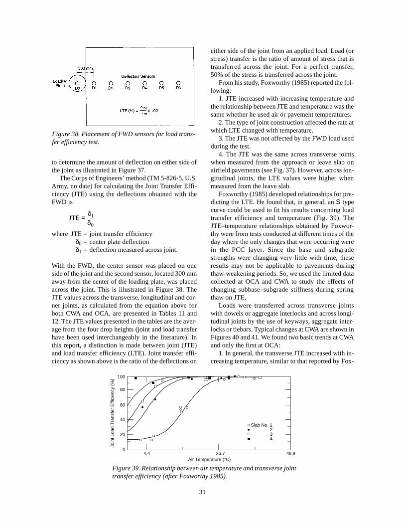
either side of the joint from an applied load. Load (orstress) transfer is the ratio of amount of stress that istransferred across the joint. For a perfect transfer,50% of the stress is transferred across the joint.
From his study, Foxworthy (1985) reported the fol-lowing:
1. JTE increased with increasing temperature andthe relationship between JTE and temperature was thesame whether he used air or pavement temperatures.
2. The type of joint construction affected the rate atwhich LTE changed with temperature.
3. The JTE was not affected by the FWD load usedduring the test.
4. The JTE was the same across transverse jointswhen measured from the approach or leave slab onairfield pavements (see Fig. 37). However, across lon-gitudinal joints, the LTE values were higher whenmeasured from the leave slab.
Foxworthy (1985) developed relationships for pre-dicting the LTE. He found that, in general, an S typecurve could be used to fit his results concerning loadtransfer efficiency and temperature (Fig. 39). TheJTE–temperature relationships obtained by Foxwor-thy were from tests conducted at different times of theday where the only changes that were occurring werein the PCC layer. Since the base and subgradestrengths were changing very little with time, theseresults may not be applicable to pavements duringthaw-weakening periods. So, we used the limited datacollected at OCA and CWA to study the effects ofchanging subbase–subgrade stiffness during springthaw on JTE.
Loads were transferred across transverse jointswith dowels or aggregate interlocks and across longi-tudinal joints by the use of keyways, aggregate inter-locks or tiebars. Typical changes at CWA are shown inFigures 40 and 41. We found two basic trends at CWAand only the first at OCA:
1. In general, the transverse JTE increased with in-creasing temperature, similar to that reported by Fox-
31
Figure 39. Relationship between air temperature and transverse jointtransfer efficiency (after Foxworthy 1985).
100
80
60
40
20
04.4 26.7 48.9
Air Temperature (°C)
Join
t Loa
d T
rans
fer
Effi
cien
cy (
%)
Slab No. 1 2 3 4
Figure 38. Placement of FWD sensors for load trans-fer efficiency test.
to determine the amount of deflection on either side ofthe joint as illustrated in Figure 37.
The Corps of Engineers’ method (TM 5-826-5, U.S.Army, no date) for calculating the Joint Transfer Effi-ciency (JTE) using the deflections obtained with theFWD is
JTE = δδ
1
0
where JTE = joint transfer efficiencyδ0 = center plate deflectionδ1 = deflection measured across joint.
With the FWD, the center sensor was placed on oneside of the joint and the second sensor, located 300 mmaway from the center of the loading plate, was placedacross the joint. This is illustrated in Figure 38. TheJTE values across the transverse, longitudinal and cor-ner joints, as calculated from the equation above forboth CWA and OCA, are presented in Tables 11 and12. The JTE values presented in the tables are the aver-age from the four drop heights (joint and load transferhave been used interchangeably in the literature). Inthis report, a distinction is made between joint (JTE)and load transfer efficiency (LTE). Joint transfer effi-ciency as shown above is the ratio of the deflections on
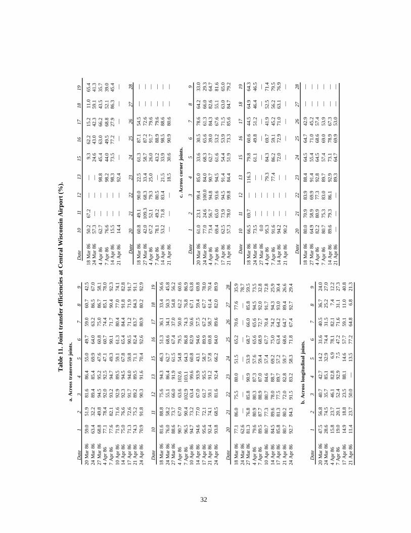
32
Dat
e10
1112
1315
1617
1819
18 M
ar 8
650
.267
.2—
—9.
362
.215
.211
.065
.424
Mar
86
57.3
——
—24
.643
.042
.359
.141
.34
Apr
86
62.7
——
98.8
45.4
63.0
66.2
43.5
35.7
7 A
pr 8
676
.6—
—98
.244
.049
.568
.852
.139
.014
Apr
86
15.5
——
98.3
73.5
77.2
27.9
86.3
45.4
21 A
pr 8
614
.4—
—92
.4—
——
——
Dat
e20
2122
2324
2526
2728
18 M
ar 8
660
.849
.190
.022
.561
.387
.154
.5—
—27
Mar
86
42.0
109.
368
.333
.458
.787
.272
.6—
—4
Apr
86
67.2
52.1
79.3
25.0
26.0
91.7
79.6
——
7 A
pr 8
678
.149
.280
.5—
43.2
88.9
79.6
——
14 A
pr 8
653
.271
.883
.421
.533
.998
.588
.6—
—21
Apr
86
——
—18
.530
.690
.980
.6—
—
c. A
cros
s co
rner
joi
nts.
Dat
e1
23
45
67
89
20 M
ar 8
661
.023
.199
.485
.033
.630
.578
.664
.233
.024
Mar
86
77.0
24.6
100.
084
.068
.365
.661
.366
.029
.34
Apr
86
73.4
56.7
94.8
90.7
62.7
39.0
84.3
82.6
64.7
7 A
pr 8
669
.465
.093
.694
.561
.653
.267
.655
.181
.617
Apr
86
62.5
73.9
94.5
91.4
54.4
53.9
71.5
63.0
65.0
21 A
pr 8
657
.378
.099
.884
.451
.973
.385
.684
.779
.2
Dat
e10
1112
1315
1617
1819
18 M
ar 8
666
.569
.7—
116.
379
.860
.644
.564
.964
.324
Mar
86
73.5
——
—61
.149
.851
.246
.446
.527
Mar
86
0.0
——
——
——
——
4 A
pr 8
695
.3—
—79
.384
.369
.741
.952
.571
.47
Apr
86
91.6
——
77.4
86.2
59.1
45.2
56.2
79.5
14 A
pr 8
694
.2—
——
72.0
72.9
71.0
63.1
76.9
21 A
pr 8
690
.2—
——
——
——
—
Dat
e20
2122
2324
2526
2728
18 M
ar 8
680
.070
.983
.988
.464
.564
.742
.9—
—27
Mar
86
64.9
58.9
69.9
91.4
55.4
71.0
45.2
——
4 A
pr 8
682
.280
.977
.392
.864
.568
.657
.4—
—7
Apr
86
80.7
75.3
83.0
89.7
57.4
69.0
53.9
——
14 A
pr 8
689
.679
.386
.192
.973
.178
.967
.3—
—21
Apr
86
——
—89
.364
.769
.953
.0—
—
Tab
le 1
1. J
oint
tra
nsfe
r ef
fici
enci
es a
t C
entr
al W
isco
nsin
Air
port
(%
).
a. A
cros
s tr
ansv
erse
joi
nts.
Dat
e1
23
45
67
89
20 M
ar 8
659
.051
.981
.686
.455
.049
.759
.060
.742
.524
Mar
86
63.4
32.2
89.4
85.4
69.9
64.0
63.2
86.5
67.0
27 M
ar 8
668
.849
.894
.595
.247
.660
.875
.086
.758
.14
Apr
86
77.1
78.4
92.0
92.5
47.1
60.7
74.4
85.1
78.0
7 A
pr 8
677
.682
.193
.294
.749
.390
.171
.790
.492
.310
Apr
86
71.9
71.6
92.9
89.5
59.1
61.3
80.4
77.0
74.1
14 A
pr 8
675
.076
.692
.394
.567
.865
.484
.491
.882
.817
Apr
86
71.3
72.6
91.7
94.0
59.8
90.5
71.2
71.9
91.7
21 A
pr 8
674
.375
.289
.289
.571
.182
.483
.784
.391
.124
Apr
86
70.9
91.8
90.3
91.6
70.4
92.6
80.9
80.2
92.9
Dat
e10
1112
1315
1617
1819
18 M
ar 8
681
.688
.875
.694
.346
.351
.336
.133
.456
.624
Mar
86
76.0
58.2
55.1
86.4
62.7
68.6
34.1
50.3
45.8
27 M
ar 8
688
.673
.766
.091
.961
.567
.437
.054
.856
.24
Apr
86
90.7
67.0
63.6
102.
654
.879
.550
.062
.260
.67
Apr
86
96.5
90.4
102.
910
3.1
64.3
86.8
74.3
76.8
86.9
10 A
pr 8
694
.773
.263
.499
.660
.882
.950
.667
.163
.814
Apr
86
94.6
77.0
67.0
93.9
43.1
94.6
57.5
59.4
69.8
17 A
pr 8
695
.672
.161
.795
.558
.789
.967
.267
.778
.021
Apr
86
92.4
74.1
59.1
91.2
57.8
69.8
58.7
61.4
70.4
24 A
pr 8
693
.868
.581
.692
.466
.284
.089
.682
.089
.9
Dat
e20
2122
2324
2526
2728
18 M
ar 8
677
.186
.075
.580
.051
.565
.270
.677
.635
.924
Mar
86
62.6
——
——
——
—78
.727
Mar
86
81.3
76.8
85.8
90.9
53.9
68.7
66.0
85.8
59.5
4 A
pr 8
679
.680
.980
.387
.357
.665
.665
.694
.573
.57
Apr
86
89.5
87.7
88.9
87.0
59.4
68.9
72.7
92.0
32.8
10 A
pr 8
680
.777
.380
.784
.657
.467
.770
.491
.772
.814
Apr
86
84.5
89.6
78.0
88.7
69.2
75.0
74.2
94.3
25.9
17 A
pr 8
685
.881
.377
.589
.757
.263
.464
.293
.030
.421
Apr
86
80.7
80.2
72.0
82.8
59.7
68.6
64.7
89.4
26.6
24 A
pr 8
692
.784
.391
.583
.258
.371
.867
.492
.729
.4
b. A
cros
s lo
ngit
udin
al j
oint
s.
Dat
e1
23
45
67
89
20 M
ar 8
647
.556
.840
.742
.714
.231
.640
.536
.724
.024
Mar
86
28.6
74.5
35.7
85.1
32.9
74.4
31.5
25.2
27.0
4 A
pr 8
615
.823
.746
.182
.86.
978
.182
.17.
412
.27
Apr
86
19.0
20.1
52.4
92.9
7.5
47.2
71.6
31.1
27.3
17 A
pr 8
614
.918
.823
.588
.114
.657
.759
.111
.040
.821
Apr
86
11.4
23.7
50.0
—13
.577
.264
.86.
821
.3

33
Table 12. Joint transfer efficiencies at OCA (%).
a. Across transverse joints.
Date 1 2 3 4 5 6 7 8 9 10 11
15 Mar 86 38.1 22.4 57.1 30.3 27.4 19.5 39.6 69.7 57.9 36.8 48.326 Mar 86 58.3 16.2 64.7 — 28.1 11.6 37.6 96.8 76.1 36.3 58.829 Mar 86 71.7 25.8 62.9 84.0 88.5 25.3 48.2 98.3 94.8 91.5 93.65 Apr 86 64.4 22.9 63.3 70.8 73.8 21.3 42.3 44.5 66.6 40.1 81.09 Apr 86 54.4 15.0 57.8 20.5 39.4 12.6 42.1 12.3 33.0 22.7 61.812 Apr 86 75.3 13.8 62.0 31.0 51.0 13.3 45.7 12.9 51.2 50.2 82.516 Apr 86 63.9 20.0 56.7 42.3 43.0 49.1 37.7 21.8 47.2 58.0 77.223 Apr 86 77.2 27.7 63.5 93.3 85.7 27.9 42.8 34.1 89.1 90.2 97.226 Apr 86 94.3 41.2 77.8 94.7 94.7 76.3 54.2 76.2 92.6 93.7 100.6
Date 12 13 14 15 16 19 20 21 22 23 24
15 Mar 86 41.4 24.1 42.2 7.1 65.8 77.2 54.4 51.0 30.5 52.3 34.026 Mar 86 66.5 21.3 65.6 18.8 80.7 92.2 59.1 55.3 40.2 61.0 50.029 Mar 86 87.6 69.4 90.7 29.6 92.3 94.8 87.1 62.0 67.9 92.4 75.55 Apr 86 74.6 37.0 48.6 14.0 78.9 91.4 65.4 54.6 76.6 30.2 75.59 Apr 86 77.4 19.7 28.5 16.9 76.3 90.9 61.2 54.2 52.6 76.5 33.412 Apr 86 82.2 18.9 36.9 — 78.6 92.2 63.6 54.1 55.7 15.7 116.216 Apr 86 75.6 36.6 41.4 29.4 63.3 89.4 66.9 56.8 50.4 28.3 21.023 Apr 86 91.3 20.4 35.3 18.0 76.8 91.2 73.7 56.9 49.7 18.0 15.026 Apr 86 92.8 67.6 94.0 89.7 89.9 — — — 58.2 45.8 81.7
b. Across longitudinal joints.
Date 1 2 3 4 5 6 7 8 9 10 11
15 Mar 86 24.9 61.2 67.7 34.8 17.7 20.1 80.7 45.9 50.6 11.0 27.429 Mar 86 16.6 73.5 86.1 83.3 17.0 27.5 98.9 72.3 87.5 15.8 46.45 Apr 86 15.8 80.1 89.0 59.6 18.7 19.6 92.8 77.8 74.7 23.3 17.912 Apr 86 11.7 82.1 83.1 89.8 17.2 14.5 99.5 84.0 49.1 17.2 18.326 Apr 86 80.1 106.4 86.3 88.1 25.0 49.4 92.9 84.3 91.6 39.5 82.5
Date 12 13 14 15 16 19 20 21 22 23 24
15 Mar 86 14.4 14.6 11.1 14.7 70.3 70.3 64.8 20.7 45.2 32.7 74.429 Mar 86 16.8 49.8 13.0 21.5 87.3 89.7 76.1 76.8 93.5 90.0 99.45 Apr 86 31.7 32.3 26.4 27.2 53.9 81.8 62.7 68.0 80.7 88.6 99.412 Apr 86 16.1 32.4 24.8 20.5 99.0 83.7 37.4 89.1 20.9 75.9 89.626 Apr 86 28.1 35.0 27.3 64.0 81.8 — — — 52.4 93.4 97.8
c. Across corner joints.
Date 1 2 3 4 5 6 7 8 9 10 11
15 Mar 86 33.6 27.2 50.7 84.9 17.5 16.6 41.3 29.3 13.8 15.6 20.929 Mar 86 52.7 76.3 53.1 90.5 32.3 13.4 63.7 87.4 42.5 75.6 52.65 Apr 86 56.0 41.8 59.2 85.5 25.3 10.2 57.4 66.1 31.0 32.6 103.612 Apr 86 47.5 26.3 49.3 36.0 13.7 6.6 42.0 17.7 47.4 33.4 40.626 Apr 86 46.9 95.8 66.7 92.4 55.3 — 68.2 91.7 90.1 85.4 70.1
Date 12 13 14 15 16 19 20 21 22 23 24
15 Mar 86 27.4 5.2 87.0 4.4 52.7 84.6 31.1 27.5 22.4 13.2 29.329 Mar 86 73.5 85.1 93.7 11.9 72.8 90.0 71.7 29.9 61.1 21.3 69.25 Apr 86 66.3 17.8 69.8 4.2 79.2 94.6 65.5 113.1 23.2 41.7 69.212 Apr 86 82.1 29.7 47.4 5.1 87.2 96.5 66.9 53.3 80.5 22.4 18.226 Apr 86 90.4 78.4 96.7 31.4 84.4 — — — 90.0 91.9 72.0
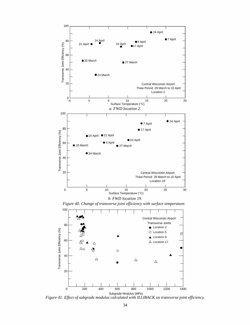
Central Wisconsin Airport
Surface Temperature (°C)
Tra
nsve
rse
Join
t Effi
cien
cy (
%)
0
20
40
60
80
100
–5 0 5 10 15 20 25
24 March
27 March
21 April 14 April 7 April
24 April
10 April17 April
4 April
20 March
Location 2 Thaw Period 29 March to 10 April
a. FWD location 2.
Figure 40. Change of transverse joint efficiency with surface temperature.
Central Wisconsin Airport
Surface Temperature (°C)
Tra
nsve
rse
Join
t Effi
cien
cy (
%)
20
40
60
80
100
0 5 10 15 20 25 30
Location 19 Thaw Period 29 March to 10 April
18 March
24 March
27 March4 April
7 April
10 April14 April
17 April
21 April
24 April
b. FWD location 19.
Figure 41. Effect of subgrade modulus calculated with ILLIBACK on transverse joint efficiency.
34
200 400 600 800 1000 1200 1400
Subgrade Modulus (MPa)
0
100
80
60
40
20
Tra
nsve
rse
Join
t Effi
cien
cy (
%)
Central Wisconsin Airport
Transverse Joints
Location 02
Location 05
Location 09
Location 17
Location 2
Location 5
Location 9
Location 17
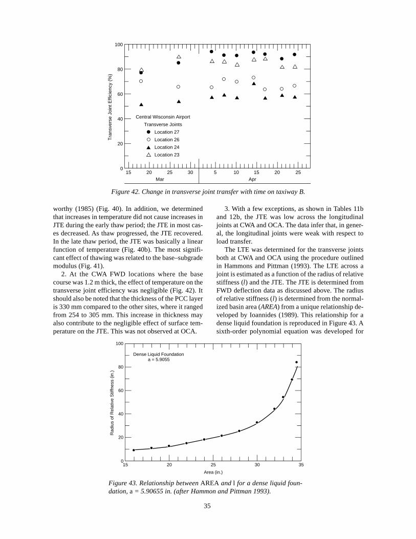
35
0
100
80
60
40
20
Tra
nsve
rse
Join
t Effi
cien
cy (
%)
15 20 25 30 5 10 15 20 25Mar Apr
Central Wisconsin Airport
Transverse Joints
Location 27
Location 26
Location 24
Location 23
Figure 42. Change in transverse joint transfer with time on taxiway B.
worthy (1985) (Fig. 40). In addition, we determinedthat increases in temperature did not cause increases inJTE during the early thaw period; the JTE in most cas-es decreased. As thaw progressed, the JTE recovered.In the late thaw period, the JTE was basically a linearfunction of temperature (Fig. 40b). The most signifi-cant effect of thawing was related to the base–subgrademodulus (Fig. 41).
2. At the CWA FWD locations where the basecourse was 1.2 m thick, the effect of temperature on thetransverse joint efficiency was negligible (Fig. 42). Itshould also be noted that the thickness of the PCC layeris 330 mm compared to the other sites, where it rangedfrom 254 to 305 mm. This increase in thickness mayalso contribute to the negligible effect of surface tem-perature on the JTE. This was not observed at OCA.
3. With a few exceptions, as shown in Tables 11band 12b, the JTE was low across the longitudinaljoints at CWA and OCA. The data infer that, in gener-al, the longitudinal joints were weak with respect toload transfer.
The LTE was determined for the transverse jointsboth at CWA and OCA using the procedure outlinedin Hammons and Pittman (1993). The LTE across ajoint is estimated as a function of the radius of relativestiffness (l) and the JTE. The JTE is determined fromFWD deflection data as discussed above. The radiusof relative stiffness (l) is determined from the normal-ized basin area (AREA) from a unique relationship de-veloped by Ioannides (1989). This relationship for adense liquid foundation is reproduced in Figure 43. Asixth-order polynomial equation was developed for
Rad
ius
of R
elat
ive
Stif
fnes
s (in
.)
15 20 25 30 35
Area (in.)
0
20
40
60
80
100
Dense Liquid Foundationa = 5.9055
Figure 43. Relationship between AREA and l for a dense liquid foun-dation, a = 5.90655 in. (after Hammon and Pittman 1993).
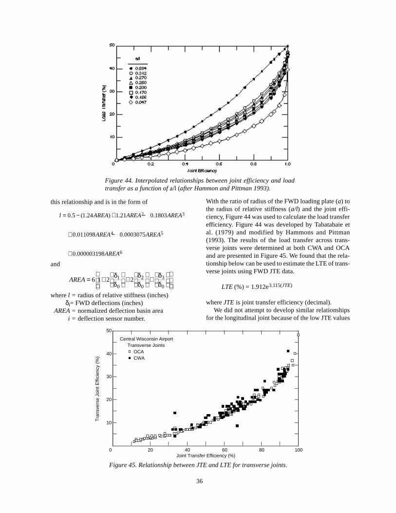
36
Figure 44. Interpolated relationships between joint efficiency and loadtransfer as a function of a/l (after Hammon and Pittman 1993).
Figure 45. Relationship between JTE and LTE for transverse joints.
Central Wisconsin Airport
OCACWA
Joint Transfer Efficiency (%)
Tra
nsve
rse
Join
t Effi
cien
cy (
%)
10
20
30
40
50
0 20 40 60 80 100
Transverse Joints
this relationship and is in the form of
l AREA AREA AREA
AREA AREA
AREA
= − + −
+ −
+
0 5 1 24 1 21 0 1803
0 011098 0 0003075
0 000003198
2 3
4 5
6
. ( . ) . .
. .
.
and
AREA = +
+
+
6 1 2 21
0
2
0
3
0
δδ
δδ
δδ
wherel = radius of relative stiffness (inches)δi= FWD deflections (inches)
AREA= normalized deflection basin areai = deflection sensor number.
With the ratio of radius of the FWD loading plate (a) tothe radius of relative stiffness (a/l) and the joint effi-ciency, Figure 44 was used to calculate the load transferefficiency. Figure 44 was developed by Tabatabaie etal. (1979) and modified by Hammons and Pittman(1993). The results of the load transfer across trans-verse joints were determined at both CWA and OCAand are presented in Figure 45. We found that the rela-tionship below can be used to estimate the LTE of trans-verse joints using FWD JTE data.
LTE (%) = 1.912e3.115(JTE)
where JTE is joint transfer efficiency (decimal).We did not attempt to develop similar relationships
for the longitudinal joint because of the low JTE values
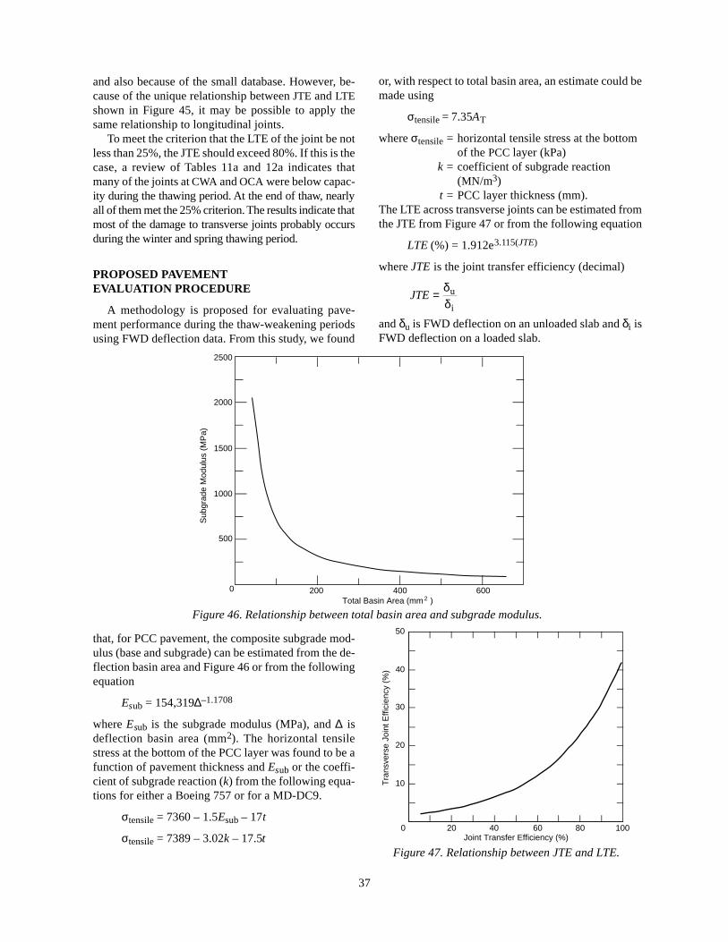
37
Joint Transfer Efficiency (%)
Tra
nsve
rse
Join
t Effi
cien
cy (
%)
10
20
30
40
50
0 20 40 60 80 100
Figure 47. Relationship between JTE and LTE.
Figure 46. Relationship between total basin area and subgrade modulus.
and also because of the small database. However, be-cause of the unique relationship between JTE and LTEshown in Figure 45, it may be possible to apply thesame relationship to longitudinal joints.
To meet the criterion that the LTE of the joint be notless than 25%, the JTE should exceed 80%. If this is thecase, a review of Tables 11a and 12a indicates thatmany of the joints at CWA and OCA were below capac-ity during the thawing period. At the end of thaw, nearlyall of them met the 25% criterion. The results indicate thatmost of the damage to transverse joints probably occursduring the winter and spring thawing period.
PROPOSED PAVEMENTEVALUATION PROCEDURE
A methodology is proposed for evaluating pave-ment performance during the thaw-weakening periodsusing FWD deflection data. From this study, we found
that, for PCC pavement, the composite subgrade mod-ulus (base and subgrade) can be estimated from the de-flection basin area and Figure 46 or from the followingequation
Esub = 154,319∆–1.1708
where Esub is the subgrade modulus (MPa), and ∆ isdeflection basin area (mm2). The horizontal tensilestress at the bottom of the PCC layer was found to be afunction of pavement thickness and Esub or the coeffi-cient of subgrade reaction (k) from the following equa-tions for either a Boeing 757 or for a MD-DC9.
σtensile = 7360 – 1.5Esub – 17t
σtensile = 7389 – 3.02k – 17.5t
or, with respect to total basin area, an estimate could bemade using
σtensile = 7.35AT
whereσtensile= horizontal tensile stress at the bottomof the PCC layer (kPa)
k = coefficient of subgrade reaction(MN/m3)
t = PCC layer thickness (mm).The LTE across transverse joints can be estimated fromthe JTE from Figure 47 or from the following equation
LTE (%) = 1.912e3.115(JTE)
where JTE is the joint transfer efficiency (decimal)
JTE = δδ
u
i
and δu is FWD deflection on an unloaded slab and δi isFWD deflection on a loaded slab.
2000
1500
1000
500
0 200 400 600
Sub
grad
e M
odul
us (
MP
a)
2500
Total Basin Area (mm )2
CMT, Inc. (1984) Pavement evaluation program—Central Wisconsin Airport.ERES Consultants (1985) Structural evaluation ofrunway 3-21.Foxworthy, P.T. (1985) Concepts for the Developmentof a Nondestructive Testing and Evaluation System forRigid Airfield Pavements. Ph.D. Dissertation, Univer-sity of Illinois at Urbana-Champaign (unpublished).Hammons M.I. and D.W. Pittman (1993) Effective-ness of load transfer devices. Draft Final Report. USAWaterways Experiment Station, Vicksburg, Mississippi.Ioannides, A.M., E.J. Barenberg and J.A. Lary (1989)Interpretation of falling weight deflectometer resultsusing principles of dimensionless analysis. AdvancedConstruction Technology Center, Document No. 89-51-01.Irwin L.H., W.S. Yang and R.N. Stubstad (1989) De-flection reading accuracy and layer thickness accuracyin backcalculation of pavement layer moduli. In Pro-ceedings, Nondestructive Testing of Pavement and Back-calculation of Moduli (A.J. Bush III and G.Y. Baladi,Ed.). ASTM STP 1026, p. 171–188.Janoo, V.C. and R.L. Berg (1990) Predicting pavementresponse during thaw weakening periods using the fall-ing weight deflectometer. In Proceedings, Third Inter-national Conference on Bearing Capacity of Roadsand Airfields, Trondheim, Norway, vol. 1, p. 31–40.Janoo, V.C. and R.L. Berg (1991) Asphalt concrete air-field pavement evaluation during thaw weakeningperiods using the falling weight deflectometer. USACold Regions Research and Engineering Laboratory,CRREL Report 91-7.Janoo, V.C. and R.L. Berg (1996) PCC airfield pave-ment response to thaw weakening periods: Data. USACold Regions Research and Engineering Laboratory,Internal Report 1155.Mead and Hunt, Inc. (1988) Runway 11/29 strength-ening design study.Stark, J. and R.L. Berg (1989) Performance of pave-ment at Central Wisconsin Airport. In Proceedings, 5thInternational Conference on Cold Regions Engineer-ing. New York: American Society of Civil Engineers.
CONCLUSIONS
During the spring thawing period, the JTE was afunction not only of the surface temperature but alsoof subgrade stiffness. Near the end of thaw, the JTEwas basically solely a function of the surface tempera-ture.
Unique relationships were developed betweenFWD deflections and the subgrade modulus (Esub)and between the FWD deflections and the coefficientof subgrade coefficient (k). Additional relationshipswere developed between the PCC layer thickness andeither Esub or k and the horizontal tensile stress (σtensile)at the bottom of the PCC layer.
A relationship was also developed for determiningthe load transfer across transverse joints on the basisof JTE calculated from FWD deflection data. This re-lationship could be also used for longitudinal joints.
The developed relationships allowed us to proposea methodology for evaluating PCC pavement perfor-mance during winter and thaw-weakening periods.However, this methodology could be used at othertimes of the year.
The relationships developed from this study shouldbe verified at other sites. In particular, although thereare only small differences in the horizontal stress rela-tionships for the Boeing 757 and the MD-DC9, addi-tional horizontal stress relationships may be neededfor other aircraft.
Field measurements of horizontal stress or strainare necessary to verify these relationships.
LITERATURE CITED
Barenberg, E.J. and A.M. Ioannides (1989) Structuralevaluation of concrete slabs using falling weight de-flectometer results, Urbana-Champaign: AdvancedConstruction Technology Center, University of Illi-nois.U.S. Army (no date) Nondestructive procedures forairfield pavement evaluation. Draft Technical ManualTM 5-826-5.
38
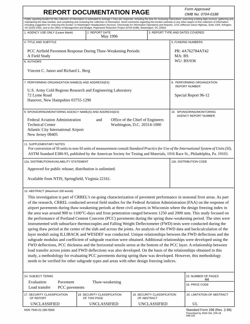
1. AGENCY USE ONLY (Leave blank) 2. REPORT DATE 3. REPORT TYPE AND DATES COVERED
4. TITLE AND SUBTITLE 5. FUNDING NUMBERS
6. AUTHORS
7. PERFORMING ORGANIZATION NAME(S) AND ADDRESS(ES) 8. PERFORMING ORGANIZATION REPORT NUMBER
9. SPONSORING/MONITORING AGENCY NAME(S) AND ADDRESS(ES) 10. SPONSORING/MONITORING AGENCY REPORT NUMBER
11. SUPPLEMENTARY NOTES
12a. DISTRIBUTION/AVAILABILITY STATEMENT 12b. DISTRIBUTION CODE
13. ABSTRACT (Maximum 200 words)
14. SUBJECT TERMS 15. NUMBER OF PAGES
16. PRICE CODE
17. SECURITY CLASSIFICATION 18. SECURITY CLASSIFICATION 19. SECURITY CLASSIFICATION 20. LIMITATION OF ABSTRACT OF REPORT OF THIS PAGE OF ABSTRACT
NSN 7540-01-280-5500 Standard Form 298 (Rev. 2-89)Prescribed by ANSI Std. Z39-18298-102
REPORT DOCUMENTATION PAGEForm ApprovedOMB No. 0704-0188
Public reporting burden for this collection of information is estimated to average 1 hour per response, including the time for reviewing instructions, searching existing data sources, gathering andmaintaining the data needed, and completing and reviewing the collection of information. Send comments regarding this burden estimate or any other aspect of this collection of information,including suggestion for reducing this burden, to Washington Headquarters Services, Directorate for Information Operations and Reports, 1215 Jefferson Davis Highway, Suite 1204, Arlington,VA 22202-4302, and to the Office of Management and Budget, Paperwork Reduction Project (0704-0188), Washington, DC 20503.
For conversion of SI units to non-SI units of measurement consult Standard Practice for Use of the International System of Units (SI),ASTM Standard E380-93, published by the American Society for Testing and Materials, 1916 Race St., Philadelphia, Pa. 19103.
May 1996
PCC Airfield Pavement Response During Thaw-Weakening Periods: PR: 4A762784AT42A Field Study MA: BS
WU: BS/036
Vincent C. Janoo and Richard L. Berg
U.S. Army Cold Regions Research and Engineering Laboratory72 Lyme Road Special Report 96-12Hanover, New Hampshire 03755-1290
Federal Aviation Administration and Office of the Chief of EngineersTechnical Center Washington, D.C. 20314-1000Atlantic City International AirportNew Jersey 08405
Approved for public release; distribution is unlimited.
Available from NTIS, Springfield, Virginia 22161.
This investigation is part of CRREL’s on-going characterization of pavement performance in seasonal frost areas. As partof the research, CRREL conducted several field studies for the Federal Aviation Administration (FAA) on the response ofairport pavements during thaw-weakening periods at three civil airports in Wisconsin where the design freezing index inthe area was around 900 to 1100°C-days and frost penetration ranged between 1250 and 2000 mm. This study focused onthe performance of Portland Cement Concrete (PCC) pavements during the spring thaw-weakening period. The sites wereinstrumented with subsurface thermocouples and Falling Weight Deflectometer (FWD) tests were conducted during thespring thaw period at the center of the slab and across the joints. An analysis of the FWD data and backcalculation of thelayer moduli using ILLIBACK and WESDEF was conducted. Unique relationships between the FWD deflections and thesubgrade modulus and coefficient of subgrade reaction were obtained. Additional relationships were developed using theFWD deflections, PCC thickness and the horizontal tensile stress at the bottom of the PCC layer. A relationship betweenload transfer across joints and FWD deflections was also developed. On the basis of the relationships obtained in thisstudy, a methodology for evaluating PCC pavements during spring thaw was developed. However, this methodologyneeds to be verified for other subgrade types and areas with other design freezing indices.
44
UNCLASSIFIED UNCLASSIFIED UNCLASSIFIED UL
Evaluation Pavement Thaw-weakeningLoad transfer PCC pavements