
PBL and precipitation interaction and grey-zone issues · PBL and precipitation interaction and...
46
PBL and precipitation interaction and grey-zone issues Song-You Hong, Hyun-Joo Choi, Ji-Young Han, and Young-Cheol Kwon (Korea Institute of Atmospheric Prediction Systems: KIAPS)
Transcript of PBL and precipitation interaction and grey-zone issues · PBL and precipitation interaction and...

PBL and precipitation interaction and grey-zone issues
Song-You Hong, Hyun-Joo Choi, Ji-Young Han,
and Young-Cheol Kwon
(Korea Institute of Atmospheric Prediction Systems: KIAPS)
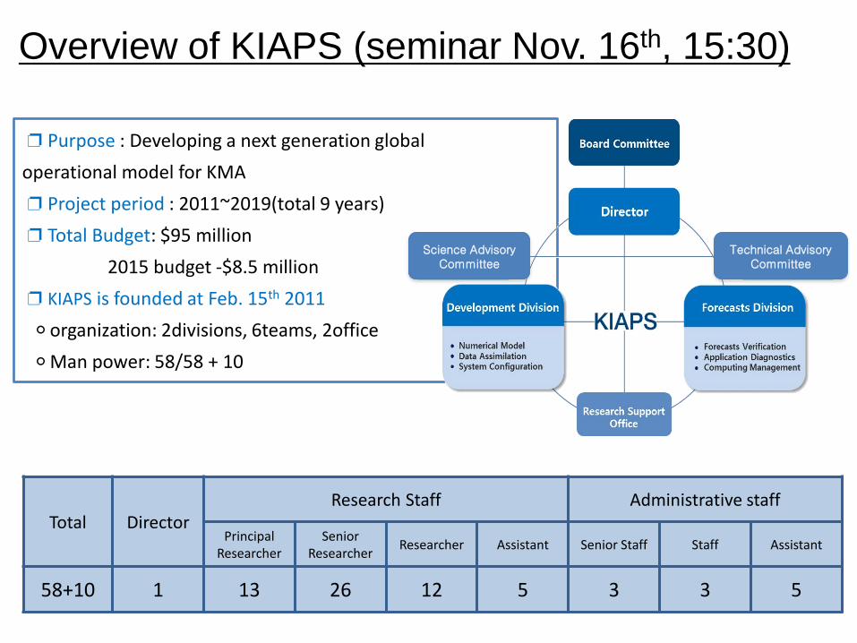
❐ Purpose : Developing a next generation global
operational model for KMA
❐ Project period : 2011~2019(total 9 years)
❐ Total Budget: $95 million
2015 budget -$8.5 million
❐ KIAPS is founded at Feb. 15th 2011
○ organization: 2divisions, 6teams, 2office
○Man power: 58/58 + 10
Overview of KIAPS (seminar Nov. 16th, 15:30)
Total DirectorResearch Staff Administrative staff
Principal Researcher
Senior Researcher
Researcher Assistant Senior Staff Staff Assistant
58+10 1 13 26 12 5 3 3 5
Science Advisory Committee
Technical Advisory Committee
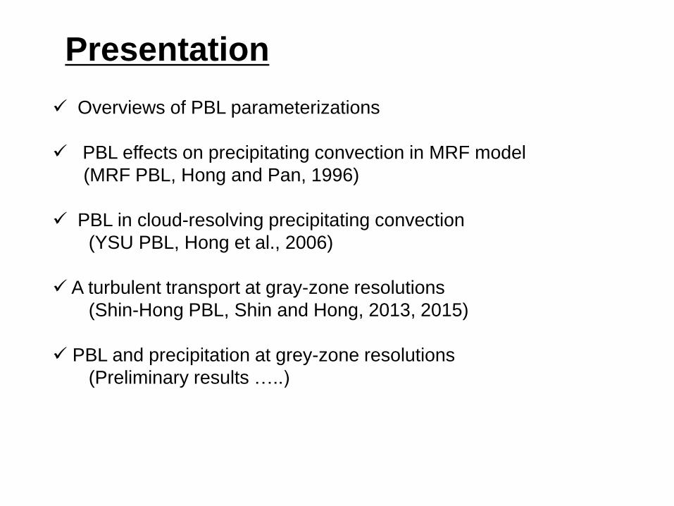
Presentation
Overviews of PBL parameterizations
PBL effects on precipitating convection in MRF model
(MRF PBL, Hong and Pan, 1996)
PBL in cloud-resolving precipitating convection
(YSU PBL, Hong et al., 2006)
A turbulent transport at gray-zone resolutions
(Shin-Hong PBL, Shin and Hong, 2013, 2015)
PBL and precipitation at grey-zone resolutions
(Preliminary results …..)
4
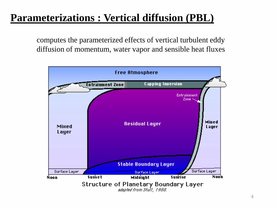
computes the parameterized effects of vertical turbulent eddy
diffusion of momentum, water vapor and sensible heat fluxes
Parameterizations : Vertical diffusion (PBL)
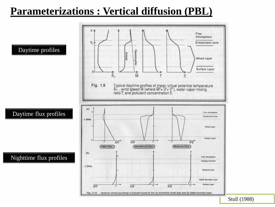
Stull (1988)
Daytime profiles
Daytime flux profiles
Nighttime flux profiles
Parameterizations : Vertical diffusion (PBL)
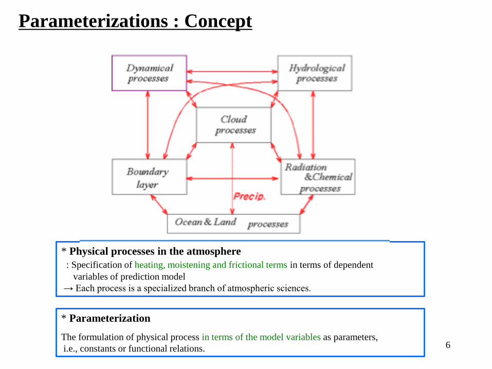
* Physical processes in the atmosphere
: Specification of heating, moistening and frictional terms in terms of dependent
variables of prediction model
→ Each process is a specialized branch of atmospheric sciences.
* Parameterization
The formulation of physical process in terms of the model variables as parameters,
i.e., constants or functional relations. 6
Parameterizations : Concept
0, 0,q u q u q u q
¶rq
¶t= -
¶ruq
¶x-
¶rvq
¶y-
¶rwq
¶z-
¶r ¢u ¢q
¶x-
¶r ¢v ¢q
¶y-
¶r ¢w ¢q
¶z+ rE - rC (2)
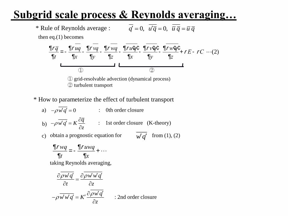
① ②
① grid-resolvable advection (dynamical process)
② turbulent transport
0w q
qw q K
z
w q
¶rwq
¶t= -
¶ruwq
¶x+
w q w w q
t z
w qw w q K
z
* Rule of Reynolds average :
then eq.(1) becomes
* How to parameterize the effect of turbulent transport
a)
b)
c) obtain a prognostic equation for
: 0th order closure
: 1st order closure (K-theory)
from (1), (2)
taking Reynolds averaging,
: 2nd order closure
Subgrid scale process & Reynolds averaging…
Local Richardson number
¶c
¶t=
¶z(-wc ) =
¶z[kc(¶c
¶z)] k
c: diffusivity, k
m,kt =l2 f
m,t(Ri)
¶U
¶z
¶uiuj
¶t+u
j
¶uiuj
¶xj
= -
¶xk
[uiujuk+
1
r]
uiuj==> k
z= fn (TKE)
¶c
¶t=
¶z(-wc ) =
¶z[kc(¶c
¶z)]+
¶z[-k
cgc]
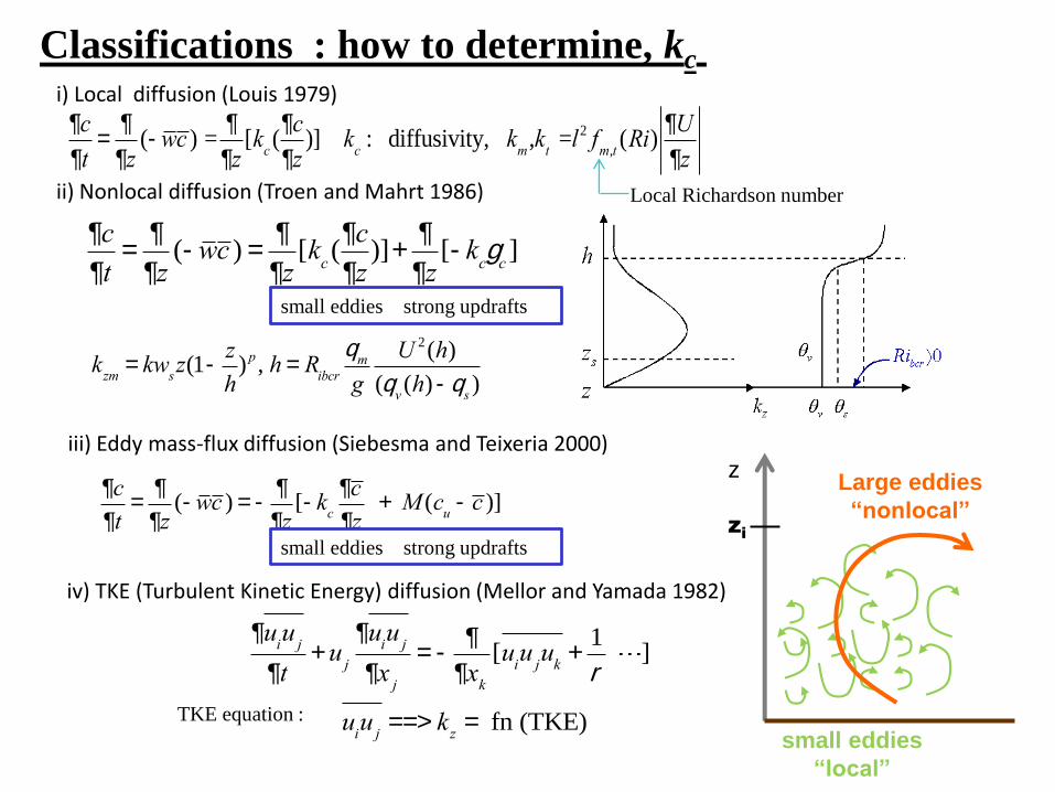
i) Local diffusion (Louis 1979)
iv) TKE (Turbulent Kinetic Energy) diffusion (Mellor and Yamada 1982)
ii) Nonlocal diffusion (Troen and Mahrt 1986)
TKE equation :
Classifications : how to determine, kc
iii) Eddy mass-flux diffusion (Siebesma and Teixeria 2000)
¶c
¶t=
¶z(-wc ) = -
¶z[-k
c
¶c
¶z + M (c
u- c )]
small eddies strong updrafts
z
zi
Large eddies
“nonlocal”
small eddies
“local”
kzm
= kwsz(1-
z
h) p , h = R
ibcr
qm
g
U 2(h)
(qv(h)-q
s)
small eddies strong updrafts
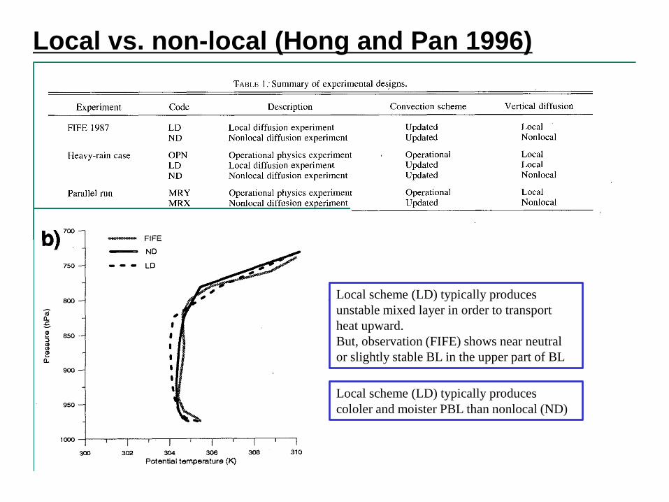
Local vs. non-local (Hong and Pan 1996)
Local scheme (LD) typically produces
unstable mixed layer in order to transport
heat upward.
But, observation (FIFE) shows near neutral
or slightly stable BL in the upper part of BL
Local scheme (LD) typically produces
cololer and moister PBL than nonlocal (ND)
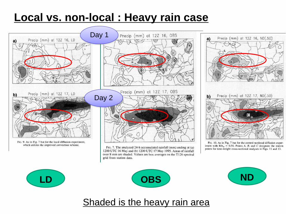
Local vs. non-local : Heavy rain case
LD OBS ND
Day 1
Day 2
Shaded is the heavy rain area
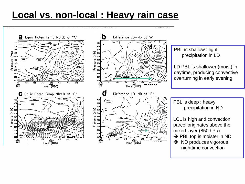
Local vs. non-local : Heavy rain case
PBL is shallow : light
precipitation in LD
LD PBL is shallower (moist) in
daytime, producing convective
overturning in early evening
PBL is deep : heavy
precipitation in ND
LCL is high and convection
parcel originates above the
mixed layer (850 hPa)
PBL top is moister in ND
ND produces vigorous
nighttime convection
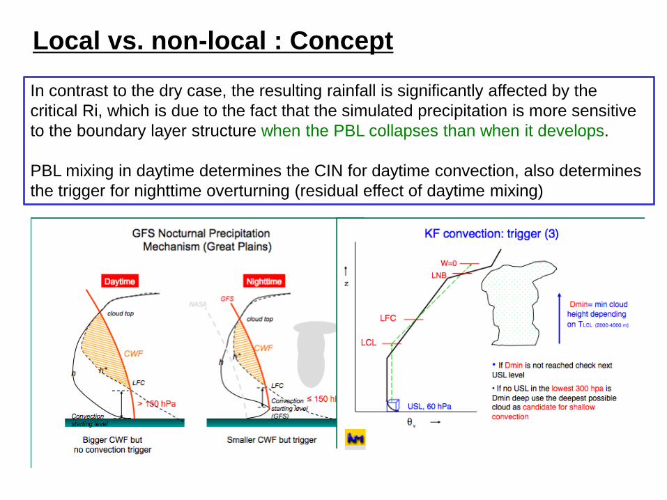
Local vs. non-local : Concept
In contrast to the dry case, the resulting rainfall is significantly affected by the
critical Ri, which is due to the fact that the simulated precipitation is more sensitive
to the boundary layer structure when the PBL collapses than when it develops.
PBL mixing in daytime determines the CIN for daytime convection, also determines
the trigger for nighttime overturning (residual effect of daytime mixing)
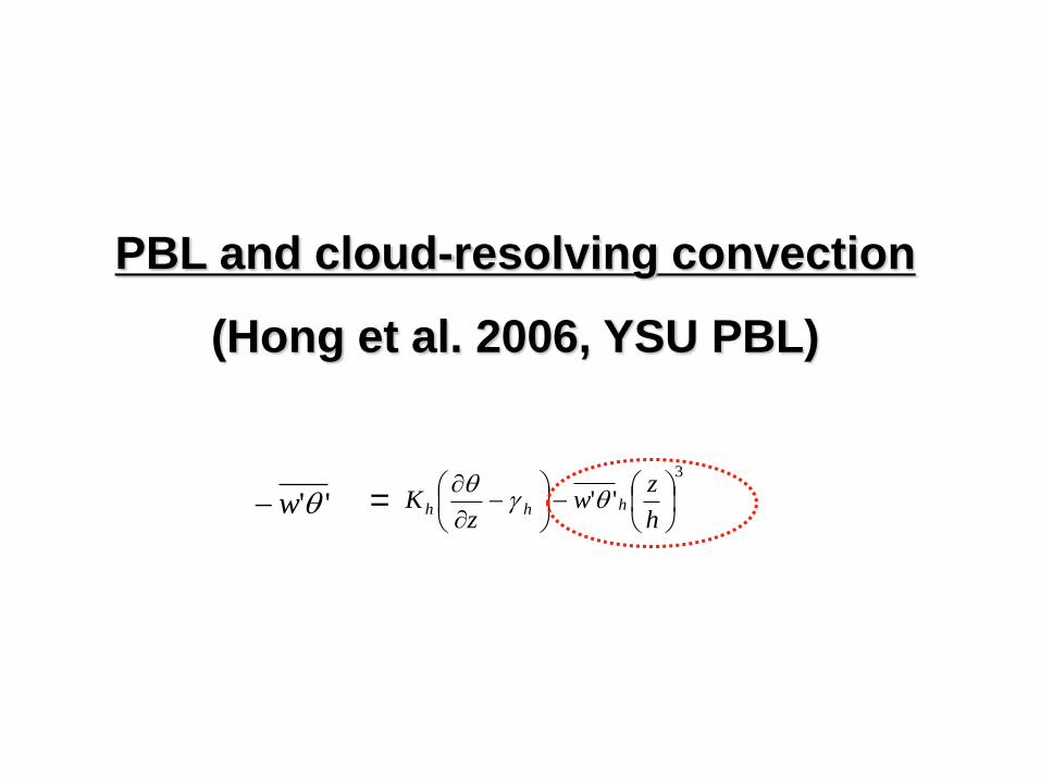
PBL and cloud-resolving convection
(Hong et al. 2006, YSU PBL)
''w
3
''
h
zw
zK hhh
=
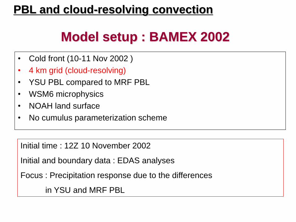
• Cold front (10-11 Nov 2002 )
• 4 km grid (cloud-resolving)
• YSU PBL compared to MRF PBL
• WSM6 microphysics
• NOAH land surface
• No cumulus parameterization scheme
Model setup : BAMEX 2002
Initial time : 12Z 10 November 2002
Initial and boundary data : EDAS analyses
Focus : Precipitation response due to the differences
in YSU and MRF PBL
PBL and cloud-resolving convection
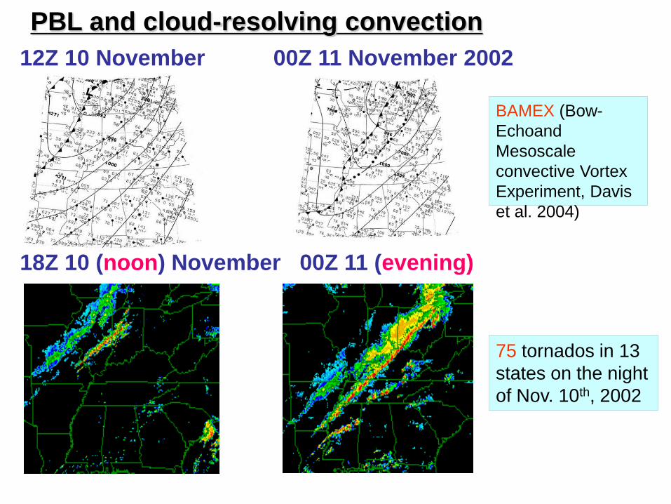
12Z 10 November 00Z 11 November 2002
18Z 10 (noon) November 00Z 11 (evening)
75 tornados in 13
states on the night
of Nov. 10th, 2002
BAMEX (Bow-
Echoand
Mesoscale
convective Vortex
Experiment, Davis
et al. 2004)
PBL and cloud-resolving convection
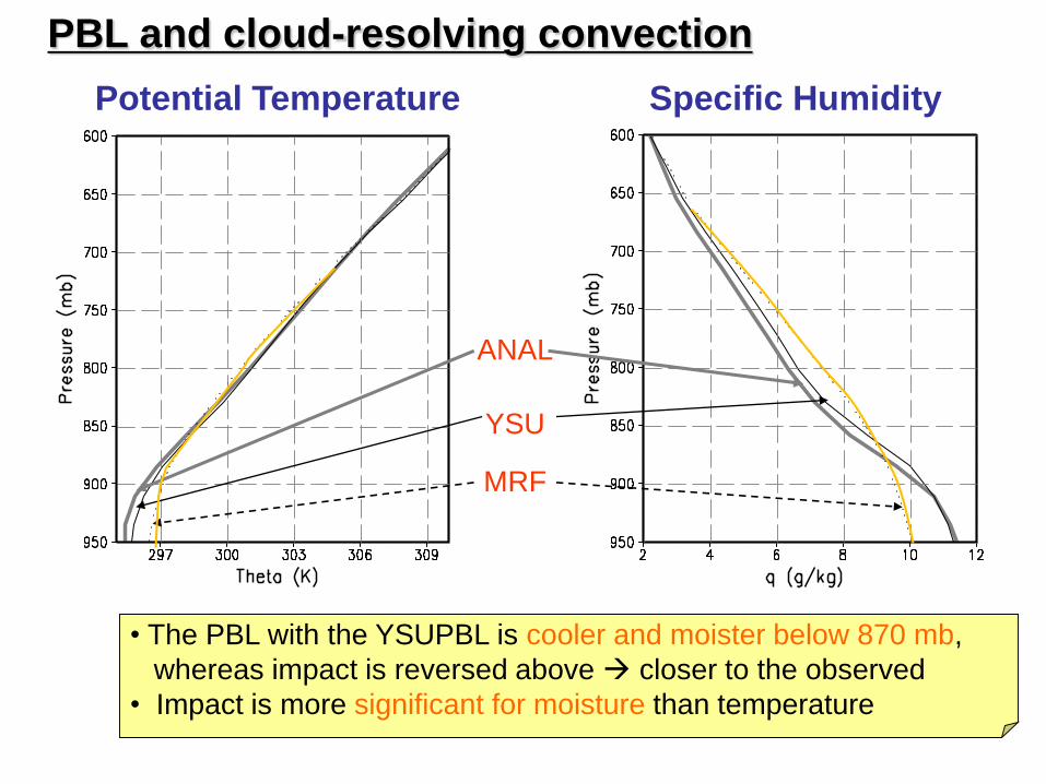
Potential Temperature Specific Humidity
YSU
MRF
ANAL
• The PBL with the YSUPBL is cooler and moister below 870 mb,
whereas impact is reversed above closer to the observed
• Impact is more significant for moisture than temperature
PBL and cloud-resolving convection
Dry convection is easy to explain, but
How can we explain the differences in precipitation ?
A
B
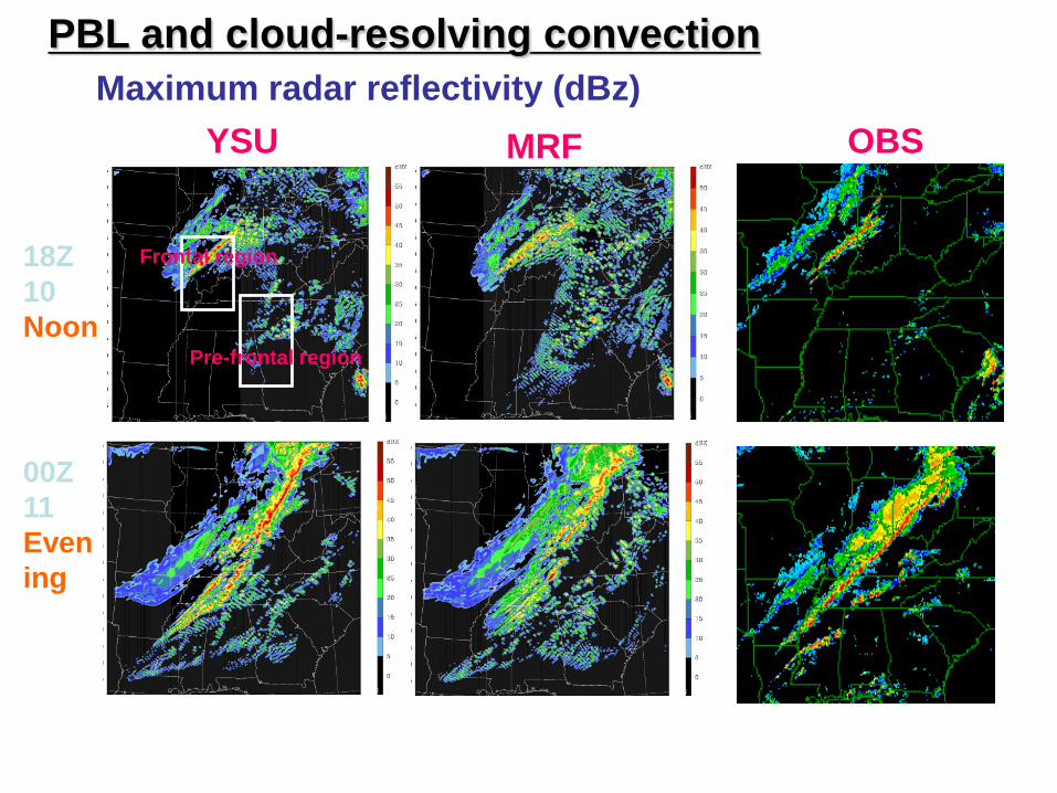
Maximum radar reflectivity (dBz)
18Z
10
Noon
00Z
11
Even
ing
YSU MRF OBS
Pre-frontal region
Frontal region
PBL and cloud-resolving convection
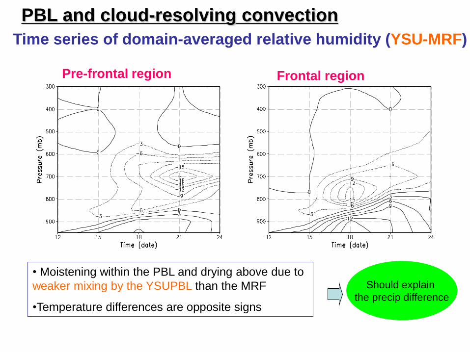
Time series of domain-averaged relative humidity (YSU-MRF)
Pre-frontal region Frontal region
• Moistening within the PBL and drying above due to
weaker mixing by the YSUPBL than the MRF
•Temperature differences are opposite signs
Should explain
the precip difference
PBL and cloud-resolving convection
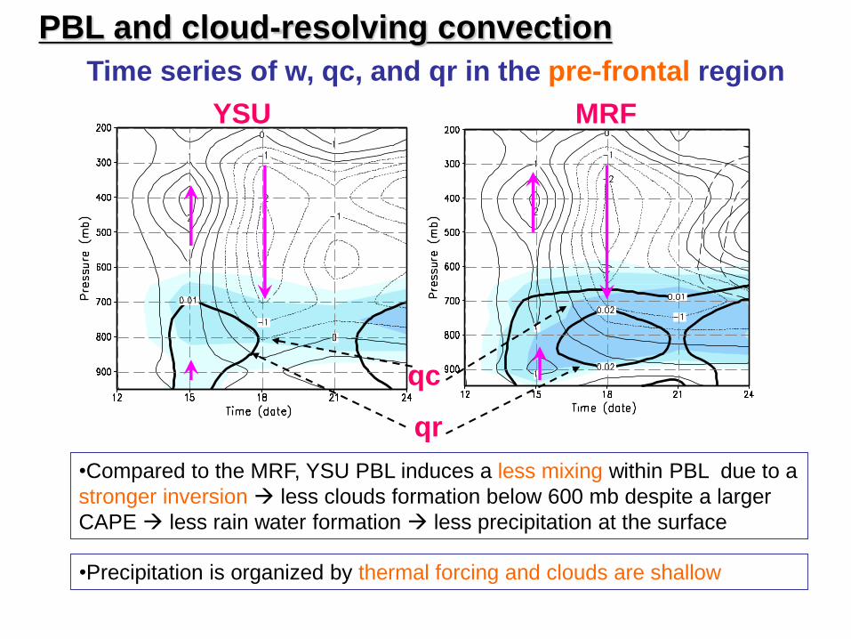
Time series of w, qc, and qr in the pre-frontal region
YSU MRF
qr
qc
•Compared to the MRF, YSU PBL induces a less mixing within PBL due to a
stronger inversion less clouds formation below 600 mb despite a larger
CAPE less rain water formation less precipitation at the surface
•Precipitation is organized by thermal forcing and clouds are shallow
PBL and cloud-resolving convection
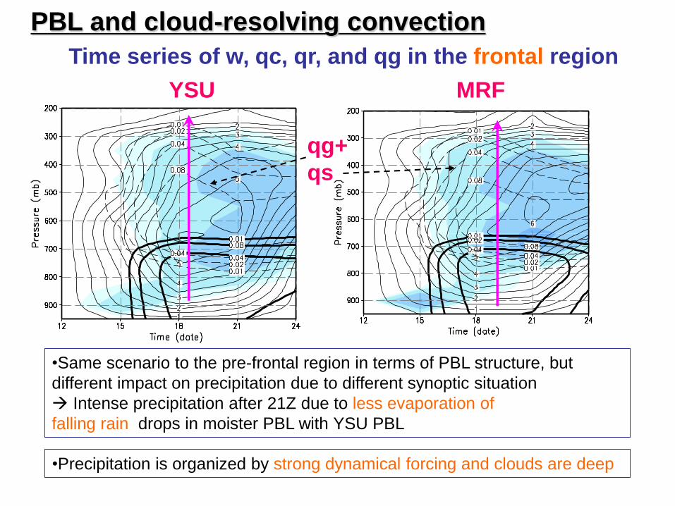
Time series of w, qc, qr, and qg in the frontal region
YSU MRF
•Same scenario to the pre-frontal region in terms of PBL structure, but
different impact on precipitation due to different synoptic situation
Intense precipitation after 21Z due to less evaporation of
falling rain drops in moister PBL with YSU PBL
•Precipitation is organized by strong dynamical forcing and clouds are deep
qg+
qs
PBL and cloud-resolving convection
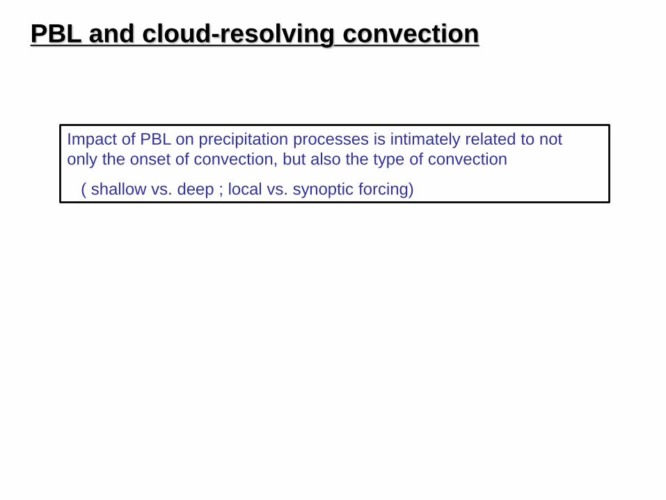
Impact of PBL on precipitation processes is intimately related to not
only the onset of convection, but also the type of convection
( shallow vs. deep ; local vs. synoptic forcing)
PBL and cloud-resolving convection
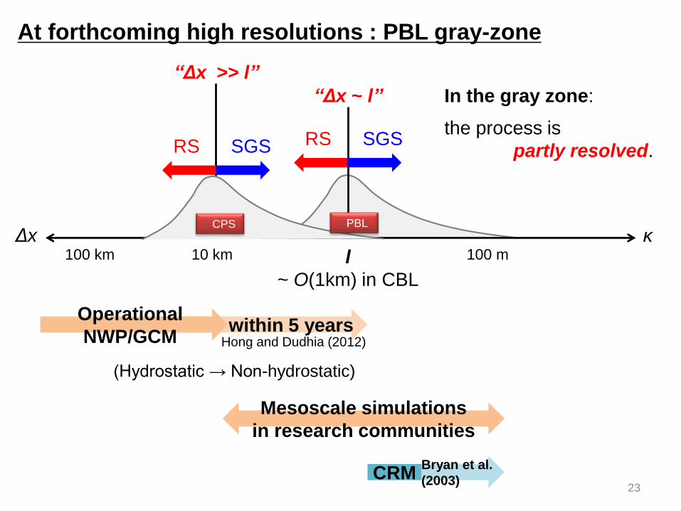
At forthcoming high resolutions : PBL gray-zone
RS SGS
“Δx ~ l”
κΔxl
~ O(1km) in CBL
10 km100 km 100 m
RS SGS
“Δx >> l”
23
In the gray zone:
the process is
partly resolved.
Mesoscale simulations
in research communities
within 5 years Operational
NWP/GCM
Bryan et al.
(2003)CRM
(Hydrostatic → Non-hydrostatic)
Hong and Dudhia (2012)
CPS PBL
24
Gray-zone PBL: Concepts & Methods
• Shin, H. H., and S.-Y. Hong, 2013: Analysis on Resolved and
Parameterized Vertical Transports in Convective Boundary Layers at
Gray-Zone Resolutions. J. Atmos. Sci., doi:10.1175/JAS-D-12-0290.1.
• Shin, H. H., and S.-Y. Hong, 2015: Representation of the Subgrid-Scal
e Turbulent Transport in Convective Boundary Layers at Gray-Zone
Resolutions. Mon. Wea. Rev.
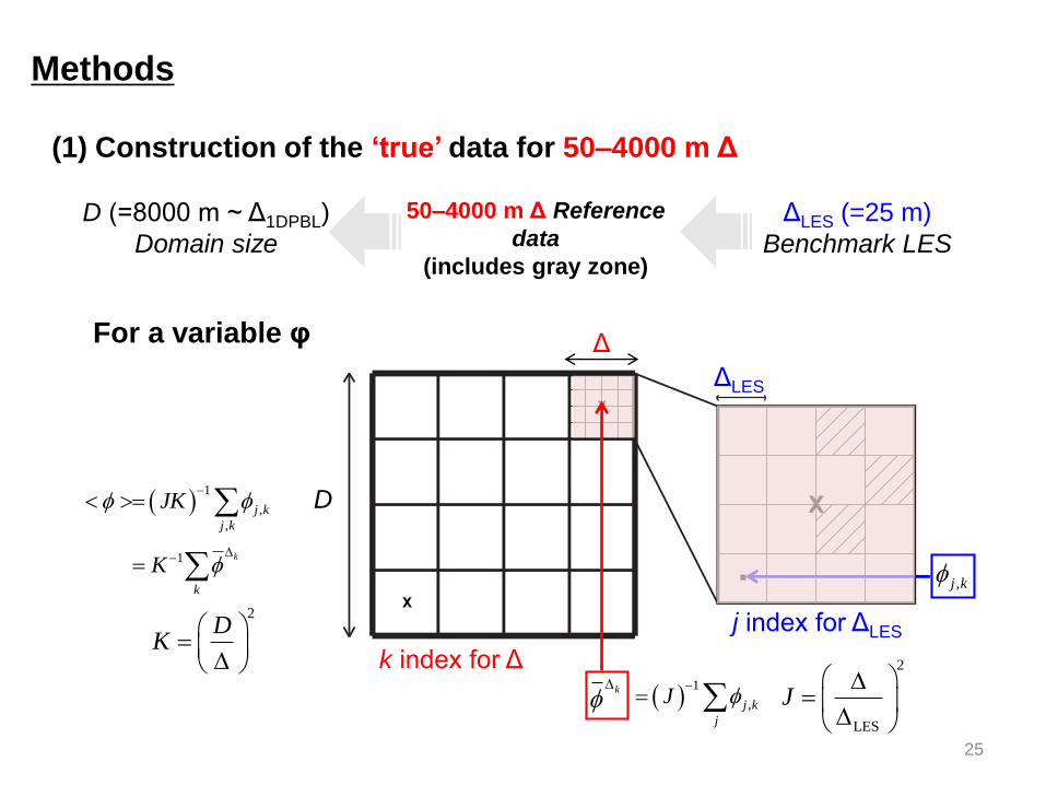
Methods
(1) Construction of the ‘true’ data for 50–4000 m Δ
ΔLES (=25 m)
Benchmark LES
50–4000 m Δ Reference
data
(includes gray zone)
D (=8000 m ~ Δ1DPBL)
Domain size
25
For a variable φ
2D
K
1 1
,
,
k
j k
j k k
JK K
1 1
,
,
k
j k
j k k
JK K
,j k
k index for Δ
j index for ΔLES
ΔLES
D
Δ
2
LES
J
1
,
k
j k
j
J
k
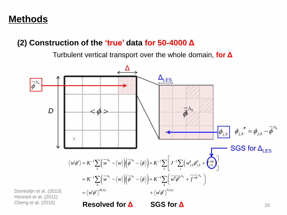
Turbulent vertical transport over the whole domain, for Δ
1 1 1
, , ,
1 1
( ) ( )
k k
kk k k
w
j k j k j k
k k j
w
k k
R S
w K w w K J w f
K w w K w f
w w
SGS for ΔLES
SGS for ΔResolved for Δ
ΔLES
D
Δ
, ,
k
j k j k
k
k
,j k
Dorrestijn et al. (2013)
Honnert et al. (2011)
Cheng et al. (2010)26
(2) Construction of the ‘true’ data for 50-4000 Δ
Methods
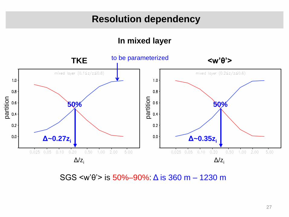
In mixed layer
27
Δ/zi
part
itio
n
Δ/zi
part
itio
n
TKE <w’θ’>
Δ~0.27zi
50%
Δ~0.35zi
50%
SGS <w’θ’> is 50%–90%: Δ is 360 m – 1230 m
to be parameterized
Resolution dependency
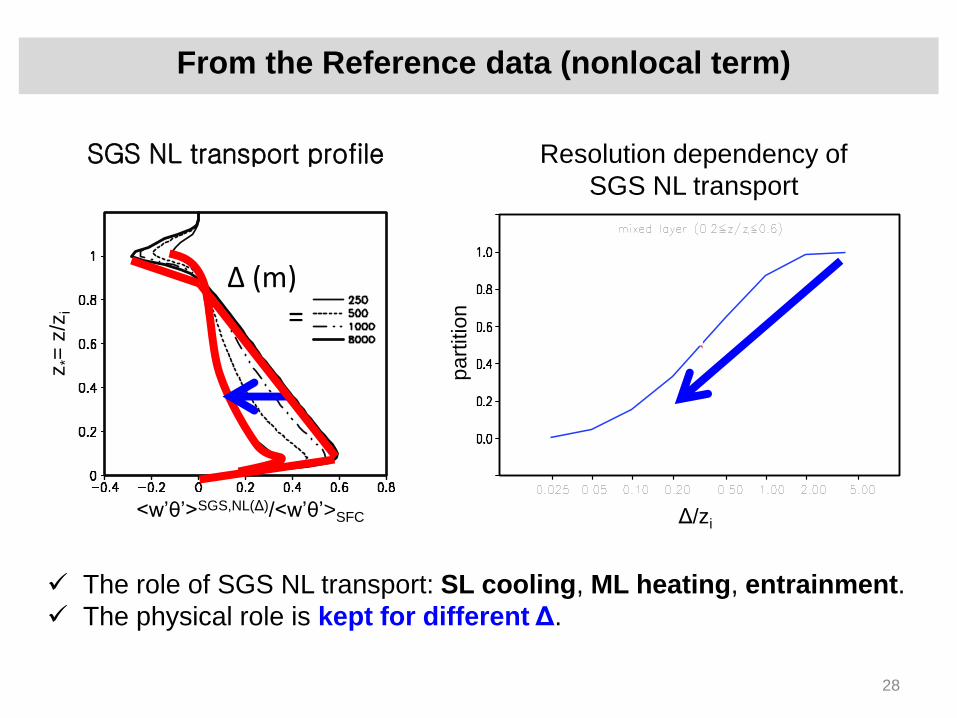
z*=
z/z
i
<w’θ’>SGS,NL(Δ)/<w’θ’>SFC
Δ (m) =
SGS NL transport profile Resolution dependency of
SGS NL transport
The role of SGS NL transport: SL cooling, ML heating, entrainment.
The physical role is kept for different Δ.
Δ/zi
part
itio
n
28
From the Reference data (nonlocal term)
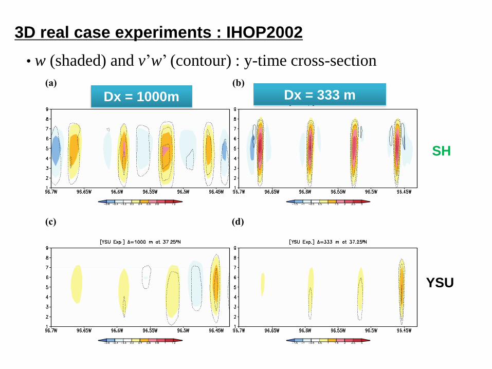
3D real case experiments : IHOP2002
• w (shaded) and v’w’ (contour) : y-time cross-section
(a) (b) 1
2
(c) (d) 3
4
SH
YSU
Dx = 1000m Dx = 333 m
PBL and precipitation at grey-zone resolutions
(YSU PBL vs. Shin-Hong PBL)
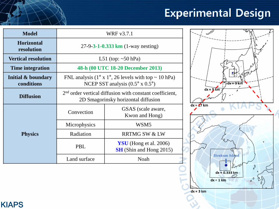
Model WRF v3.7.1
Horizontal
resolution27-9-3-1-0.333 km (1-way nesting)
Vertical resolution L51 (top: ~50 hPa)
Time integration 48-h (00 UTC 18-20 December 2013)
Initial & boundary
conditions
FNL analysis (1° x 1°, 26 levels with top ~ 10 hPa)
NCEP SST analysis (0.5° x 0.5°)
Diffusion2nd order vertical diffusion with constant coefficient,
2D Smagorinsky horizontal diffusion
Physics
ConvectionGSAS (scale aware,
Kwon and Hong)
Microphysics WSM5
Radiation RRTMG SW & LW
PBLYSU (Hong et al. 2006)
SH (Shin and Hong 2015)
Land surface Noah
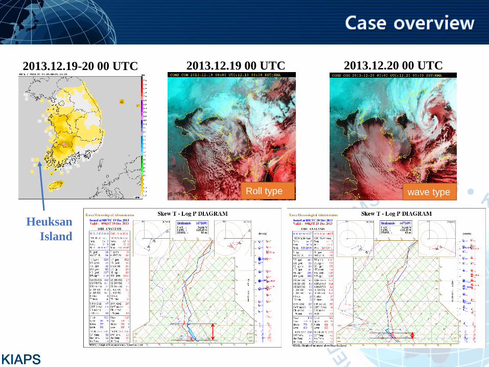
2013.12.19-20 00 UTC 2013.12.19 00 UTC 2013.12.20 00 UTC
Heuksan
Island
Roll type wave type
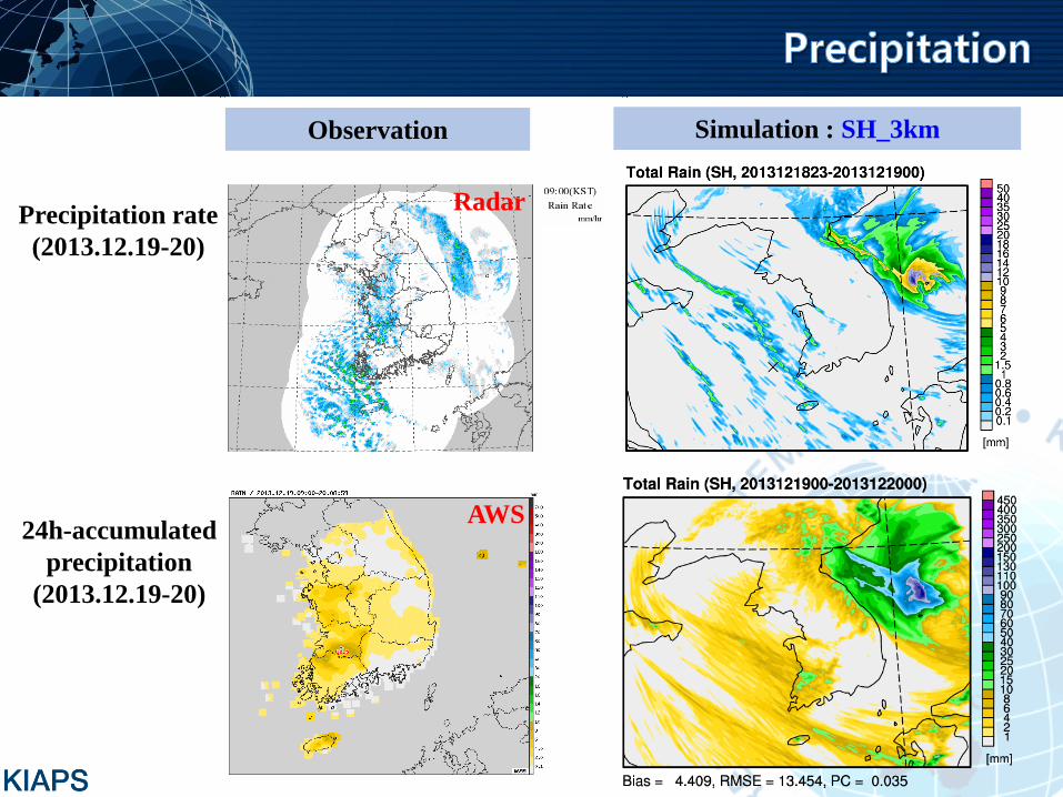
Simulation : SH_3km
24h-accumulated
precipitation
(2013.12.19-20)
Observation
Precipitation rate
(2013.12.19-20)
Radar
AWS
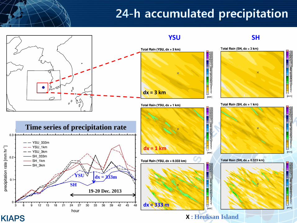
YSU SH
dx = 3 km
X : Heuksan Island
dx = 1 km
dx = 333 m
Time series of precipitation rate
19-20 Dec. 2013
dx = 333m
SH
YSU
dx = 3 km
X : Heuksan Island
dx = 1 km
dx = 333 m
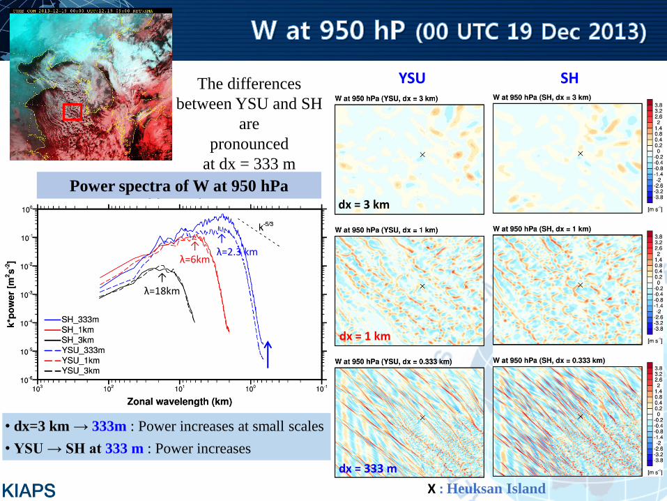
YSU SH
Power spectra of W at 950 hPa
• dx=3 km → 333m : Power increases at small scales
• YSU → SH at 333 m : Power increases
↑λ=18km
↑λ=6km
↑λ=2.3 km
The differences
between YSU and SH
are
pronounced
at dx = 333 m
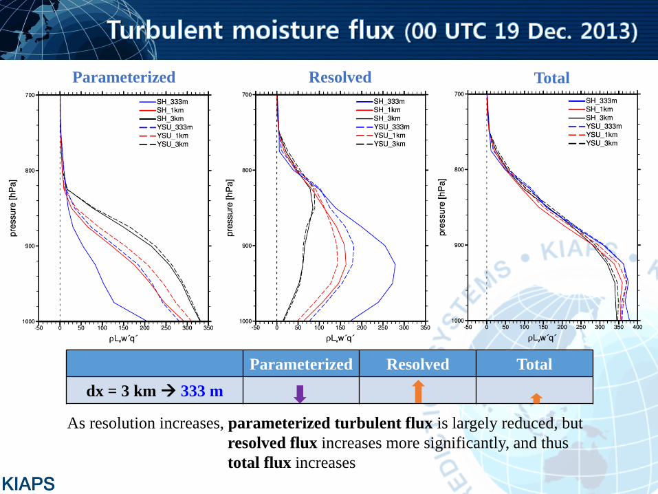
Parameterized Resolved
Parameterized Resolved Total
dx = 3 km 333 m
Total
As resolution increases, parameterized turbulent flux is largely reduced, but
resolved flux increases more significantly, and thus
total flux increases
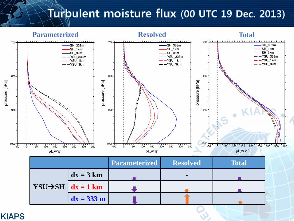
Parameterized Resolved
Parameterized Resolved Total
YSUSH
dx = 3 km -
dx = 1 km
dx = 333 m
Total
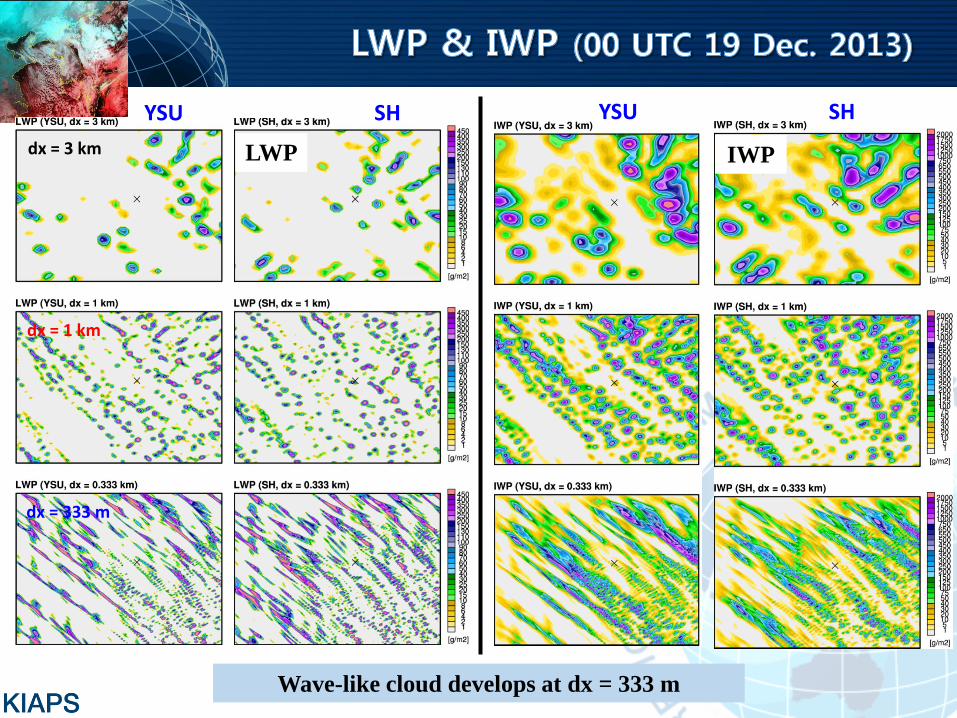
IWPLWP
YSU SH YSU SH
dx = 3 km
dx = 1 km
dx = 333 m
Wave-like cloud develops at dx = 333 m
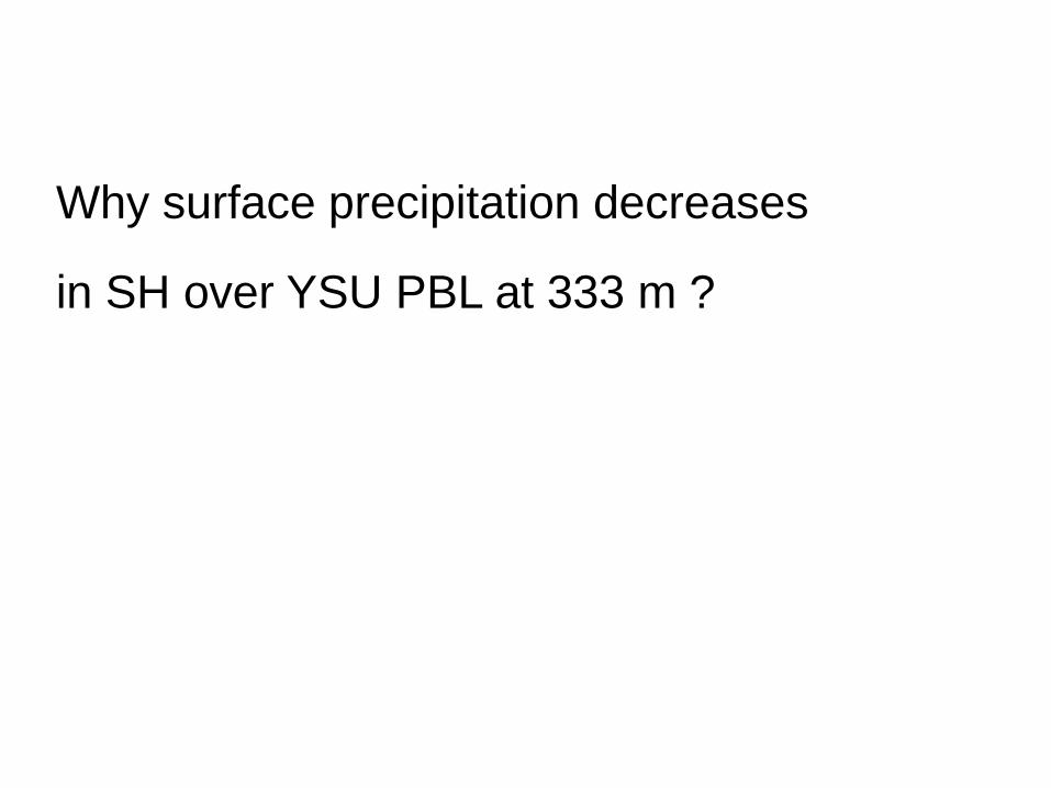
Why surface precipitation decreases
in SH over YSU PBL at 333 m ?
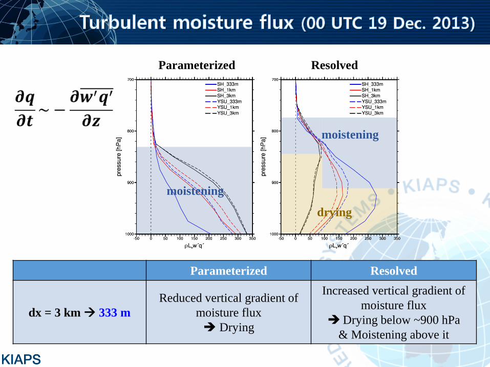
Parameterized Resolved
Parameterized Resolved
dx = 3 km 333 m
Reduced vertical gradient of
moisture flux
Drying
Increased vertical gradient of
moisture flux
Drying below ~900 hPa
& Moistening above it
moistening
moistening
drying
drying
moistening
moistening
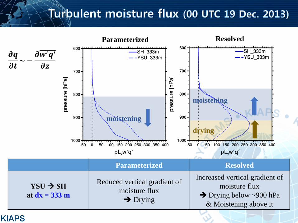
Parameterized Resolved
Parameterized Resolved
YSU SH
at dx = 333 m
Reduced vertical gradient of
moisture flux
Drying
Increased vertical gradient of
moisture flux
Drying below ~900 hPa
& Moistening above it
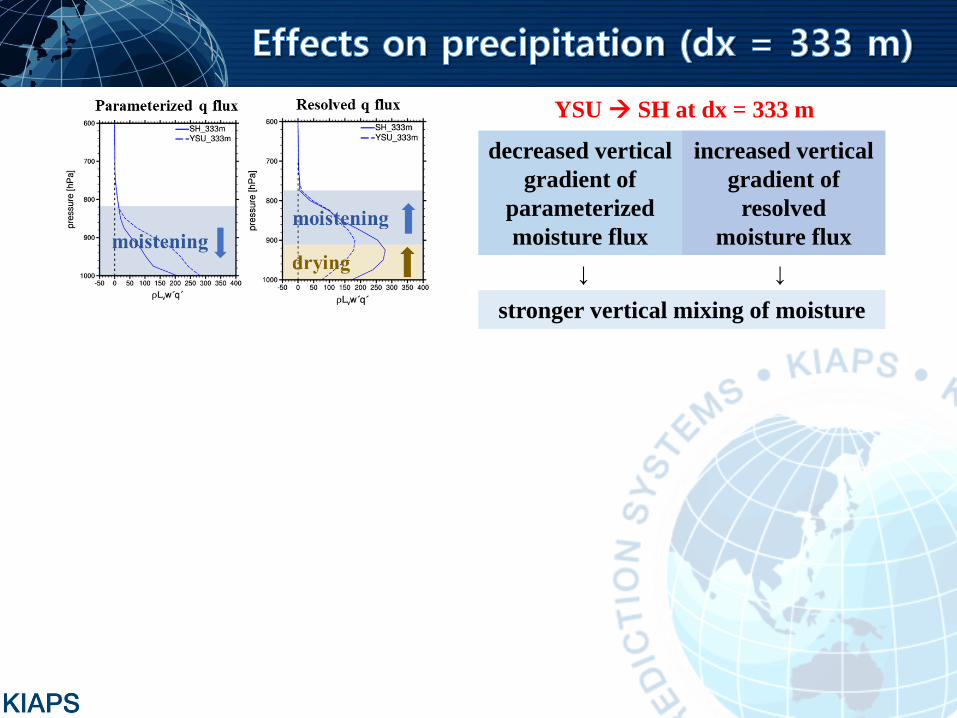
YSU SH at dx = 333 m
decreased vertical
gradient of
parameterized
moisture flux
increased vertical
gradient of
resolved
moisture flux
↓ ↓
stronger vertical mixing of moisture
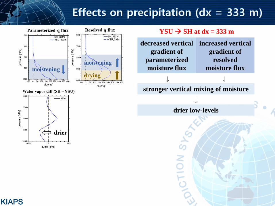
YSU SH at dx = 333 m
decreased vertical
gradient of
parameterized
moisture flux
increased vertical
gradient of
resolved
moisture flux
↓ ↓
stronger vertical mixing of moisture
↓
drier low-levels
drier
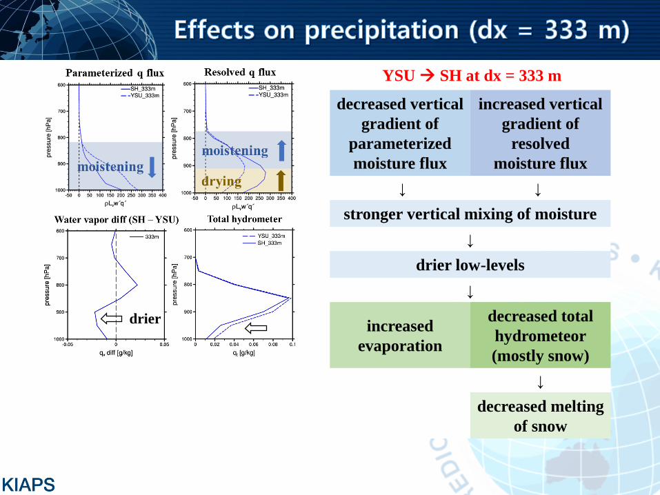
YSU SH at dx = 333 m
decreased vertical
gradient of
parameterized
moisture flux
increased vertical
gradient of
resolved
moisture flux
↓ ↓
stronger vertical mixing of moisture
↓
drier low-levels
↓
increased
evaporation
decreased total
hydrometeor
(mostly snow)
↓
decreased melting
of snow
drier
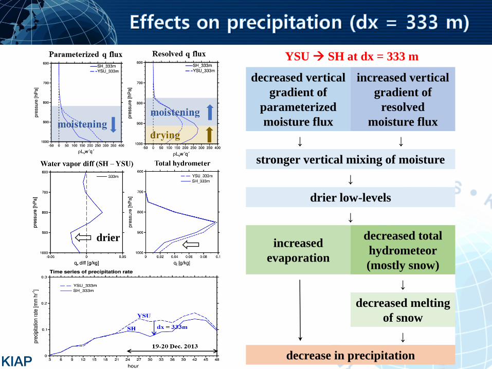
YSU SH at dx = 333 m
decreased vertical
gradient of
parameterized
moisture flux
increased vertical
gradient of
resolved
moisture flux
↓ ↓
stronger vertical mixing of moisture
↓
drier low-levels
↓
increased
evaporation
decreased total
hydrometeor
(mostly snow)
↓
decreased melting
of snow
↓
decrease in precipitation
drier