Paying for Safety:An Economic Analysis of the Effect ofCompensation on Truck Driver Safety

Michael H. Belzer*Project Director and Principal Investigator

Daniel Rodriguez**Investigator

Stanley A. Sedo***Investigator

September 10, 2002

Direct SponsorScience Applications International Corporation

Prime SponsorFederal Motor Carrier Safety AdministrationPrime Contract Number DTFH 61-98-C-0061

* Associate ProfessorCollege of Urban, Labor, and Metropolitan Affairs

Wayne State Universityand

Research ScientistInstitute of Labor and Industrial Relations

University of Michigan

** Assistant ProfessorDepartment of City and Regional PlanningUniversity of North Carolina, Chapel Hill

***Assistant Research ScientistInstitute of Labor and Industrial Relations

and LecturerEconomics DepartmentUniversity of Michigan

Address all correspondence to:

Michael H. BelzerAssociate Professor

College of Urban, Labor, and Metropolitan AffairsWayne State University

3198 Faculty/Administration Building656 W. Kirby

Detroit, MI 48202Phone: 313-577-1328Fax: 313-577-8800

E-mail: Michael.H.Belzer@wayne.edu

2

TABLE OF CONTENTSExecutive Summary..........................................................................................................................6

I. Introduction...............................................................................................................................15

II. Literature Review.....................................................................................................................17Introduction............................................................................................................................................17

Motivation...............................................................................................................................................17

The Role of Employee Compensation..................................................................................................18

Compensation Level...............................................................................................................................19Direct Compensation............................................................................................................................................19Efficiency wages..................................................................................................................................................20Wage-deferral or wage-tilting..............................................................................................................................20Transaction cost theory........................................................................................................................................21Incentive theory....................................................................................................................................................21Equalizing differences theory..............................................................................................................................22Fair wage theory...................................................................................................................................................22

Compensation Method...........................................................................................................................22Direct Compensation............................................................................................................................................23Deferred Compensation.......................................................................................................................................24

III: Driver Compensation and Driver Safety: Evidence from Trucking Research....................27Safety Studies of the Trucking Industry: Firm-Level Characteristics.............................................27

Firm profitability..................................................................................................................................................28Specific Firm Safety Practices.............................................................................................................................29Fleet Ownership...................................................................................................................................................29Demographics of firm driver force......................................................................................................................30Firm age...............................................................................................................................................................30Union presence.....................................................................................................................................................30Firm size...............................................................................................................................................................31Industry segment..................................................................................................................................................31Summary..............................................................................................................................................................31

Empirical Evidence for the Effect of Methods and Level of Compensation in the Trucking Industry: Driver-Level Research..........................................................................................................32

Other Issues in the Relationship Between Driver Compensation and Safety..................................34

Indirect Links Between Driver Compensation and Driver Safety....................................................35

Indirect Effects, Compensation Level and Method............................................................................36

Indirect Effects, Driver Safety..............................................................................................................37Age.......................................................................................................................................................................37Work experience..................................................................................................................................................37Fatigue..................................................................................................................................................................38Turnover...............................................................................................................................................................39Safety Climate......................................................................................................................................................39

Driver Safety and Driver Crashes........................................................................................................39

IV. DATA......................................................................................................................................41

3

UMTIP Drivers Survey.........................................................................................................................42

National Survey of Driver Wages.........................................................................................................43

SAFER Web Site....................................................................................................................................44

MCMIS Crash File................................................................................................................................44

MCMIS Carrier Profiles.......................................................................................................................45

Financial and Operating Statistics Form M Data...............................................................................45

Firm-Specific Case Studies....................................................................................................................46

V. RESEARCH STRATEGIES....................................................................................................47Theoretical Background........................................................................................................................47

The Standard Model.............................................................................................................................................47Extensions of the Standard Model.......................................................................................................................49

Theoretical Arguments: The Tradeoff between Pay Rate and Hours of Work...............................52Labor Supply Curve Estimation...........................................................................................................................54

Firm Level Data.....................................................................................................................................60

Individual Level Survey Data...............................................................................................................62

Quantitative Firm Case Study at the Individual Driver Level..........................................................62

Estimation Techniques..........................................................................................................................63

VI. RESULTS................................................................................................................................64Pay Level and Method, Cross Sectional Analysis...............................................................................64

Data......................................................................................................................................................................64Results..................................................................................................................................................................64

Pay Level and Safety: The Case of a Large Pay Raise.......................................................................71Hazard Rate..........................................................................................................................................................74Incorporation of Unobserved Heterogeneity........................................................................................................75Data......................................................................................................................................................................75Crash modeling....................................................................................................................................................78

TL Case Study: Turnover Analysis......................................................................................................88

Event: Leave the firm = 1......................................................................................................................89

The University of Michigan Trucking Industry Program Driver Survey........................................92

VII. CONCLUSIONS...................................................................................................................99Labor Supply Curve..............................................................................................................................99

Signpost...................................................................................................................................................99

J.B. Hunt.................................................................................................................................................99

Driver Survey.......................................................................................................................................100

VIII. BIBLIOGRAPHY..............................................................................................................101

Appendix A..................................................................................................................................112

Appendix B..................................................................................................................................115

4

5

FiguresFigure 1. Direct and Indirect Effects — Compensation Method and Level................35Figure 2: The Standard Model..................................................................................48Figure 3: Extension of the Standard Model...............................................................50Figure 4: Method of Pay............................................................................................51Figure 5: Labor Supply Curve for Over-the-Road Truck Drivers................................53Figure 6: Predicted Crashes......................................................................................70Figure 7: Kaplan-Meier Empirical Crash Hazard........................................................78Figure 8: Elasticity of Crash Probabilities by Pay Rate and Tenure...........................82Figure 9: Crash Risk and Age....................................................................................84Figure 10: Crash Risk and Tenure.............................................................................84Figure 11: Negative Duration Dependence and the Role of Experience...................85Figure 12: Effect of total experience on crash risk...................................................86Figure 13: Raw Turnover Risk...................................................................................89Figure 14: Turnover Probability by Driver Age..........................................................90Figure 15: Turnover Probability by Driver Tenure.....................................................91Figure 16: Estimated Semi-Parametric Baseline Turnover Hazard...........................92

TablesTable 1: Summary Statistics.....................................................................................58Table 2: Mileage Rate Equation................................................................................59Table 3: Weekly Hours Equation...............................................................................60Table 4: Summary Statistics.....................................................................................65Table 5: Negative Binomial Regression Results........................................................69Table 6. Descriptive statistics summarized at the individual level..........................76Table 7: Descriptive statistics summarized at the individual level before and after

pay raise............................................................................................................77Table 8 Driver Discrete Time Proportional Crash Hazards Model with Gaussian-

Distributed Unobserved Heterogeneity..............................................................80Table 9 Driver Discrete Time Proportional Crash Hazards Model with Gaussian-

Distributed Unobserved Heterogeneity –Months of Experience Subset..............86Table 10: Driver Discrete Time Proportional Crash Hazards Model with Gaussian-

Distributed Unobserved Heterogeneity –Months of Experience AND Moving Violations Subsets..............................................................................................88

Table 11: Driver Discrete Time Proportional Turnover Hazards Model with Gaussian-Distributed Unobserved Heterogeneity..............................................................89

Table 12: Summary Statistics: Drivers’ Survey.........................................................94Table 13: Probit Results: Drivers’ Survey.................................................................97

6

Executive Summary

Paying for Safety:An Economic Analysis of the Effect of Pay on Truck Driver Safety

Michael H. Belzer, Project Director and Principal InvestigatorDaniel Rodriguez, InvestigatorStanley A. Sedo, Investigator

Address all correspondence to:

Michael H. BelzerAssociate Professor

College of Urban, Labor, and Metropolitan AffairsWayne State University

3198 Faculty/Administration Building656 W. Kirby

Detroit, MI 48202Phone: 313-577-1328Fax: 313-577-8800

E-mail: Michael.H.Belzer@wayne.edu

May 1, 2002

Direct SponsorScience Applications International Corporation

Prime SponsorFederal Highway Administration / Federal Motor Carrier Safety Administration

Prime Contract Number DTFH 61-98-C-0061

This report examines the link between truck driver pay and driver safety. It establishes a relationship that is important for policy purposes because it suggests that low driver pay, which we expect is linked to low but unmeasured human capital, may be an important predictor of truck driver safety. The study uses three different data sets at three different levels of analysis to demonstrate this link. The study also includes an estimation of the truck driver labor supply curve, an important contribution to understanding drivers’ (and carriers’) preferences for balancing income and work time. One model includes the entire population of drivers at a very large truckload motor carrier and uses survival analysis (also known as duration modeling) to measure individual crash probabilities over time while controlling for individual and work characteristics. Another model uses a cross section of more than 100 truckload carriers to link driver pay with safety performance across firms. The third model uses a representative sample of individual drivers across all firms engaged in over-the-road operations to demonstrate the effect of driver pay in predicting crashes.

7

Previous Research

Research has shown that:

Over-the-road drivers ordinarily are paid on a piecework basis; Real pay levels for trucking industry personnel have declined over the past two decades; real

pay levels have declined relative to employees in other industries; Benefits availability and level of benefits have declined, and deferred compensation in the

form of pensions has declined; Unionization has declined, further reducing compensation; The trucking industry has been increasingly competitive and firms and drivers are under

great pressure to deliver loads just-in-time and quickly.

Theory

We expect driver compensation to predict safety outcomes because:

Employee earnings levels affect the quality of drivers attracted to the job; Employee expected earning levels also determine the quality of the drivers attracted to the

job; both earnings levels and expected earnings affect employee behavior; Employee pay methods affect employee behavior; Turnover, a likely independent predictor of safety, is related to compensation.

Economic theory would lead us to predict that low pay levels would be associated with low human capital and lower human capital would be associated with inferior performance outcomes. We hypothesize that low human capital is associated with unsafe driving, since higher quality workers can be expected to perform better in their jobs and since safe driving is an important attribute of high performing truck drivers.

8

Data

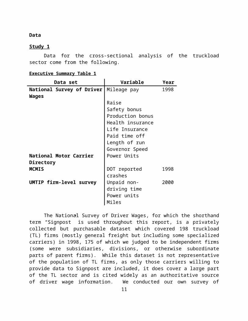
Study 1

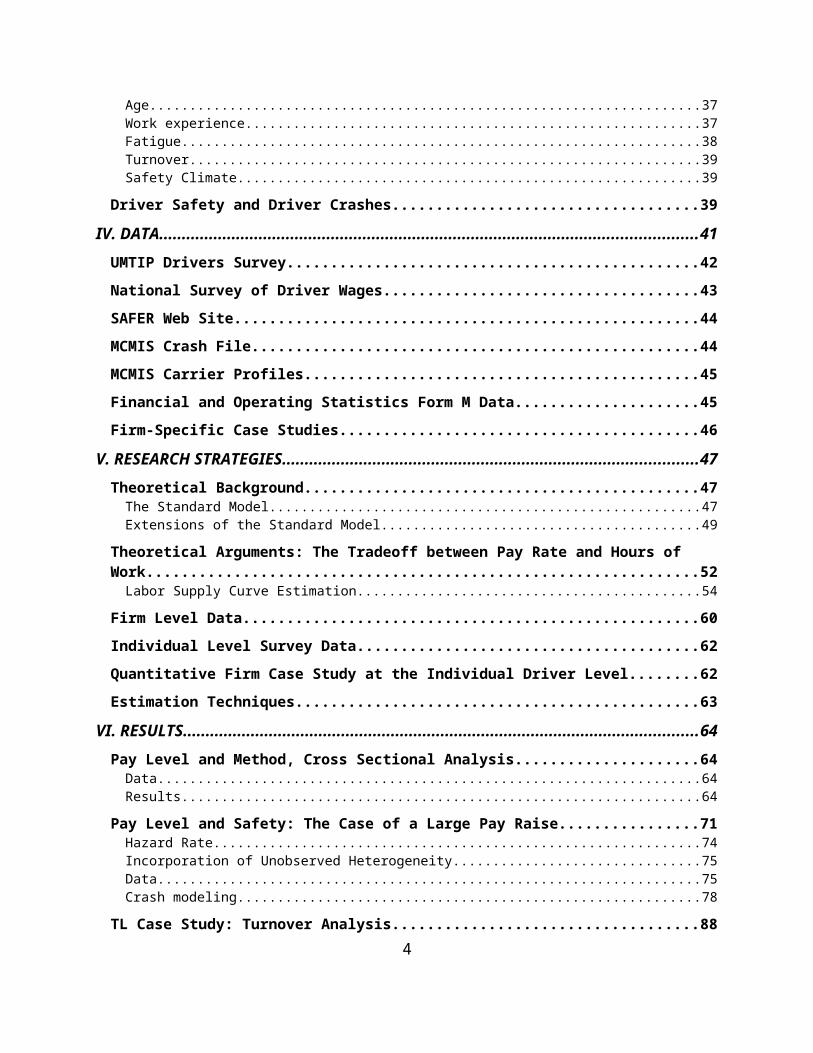
Data for the cross-sectional analysis of the truckload sector come from the following.

Executive Summary Table 1

Data set Variable YearNational Survey of Driver Wages Mileage pay 1998

RaiseSafety bonusProduction bonusHealth insuranceLife InsurancePaid time offLength of runGovernor Speed

National Motor Carrier Directory Power UnitsMCMIS DOT reported crashes 1998UMTIP firm-level survey Unpaid non-driving time 2000

Power unitsMiles

The National Survey of Driver Wages, for which the shorthand term “Signpost” is used throughout this report, is a privately collected but purchasable dataset which covered 198 truckload (TL) firms (mostly general freight but including some specialized carriers) in 1998, 175 of which we judged to be independent firms (some were subsidiaries, divisions, or otherwise subordinate parts of parent firms). While this dataset is not representative of the population of TL firms, as only those carriers willing to provide data to Signpost are included, it does cover a large part of the TL sector and is cited widely as an authoritative source of driver wage information. We conducted our own survey of Signpost firms to develop a measure of unpaid non-driving time, since Signpost declined to collect this information systematically on the presumption that drivers simply are not paid for this time (which we found not to be true). The UMTIP firm-level survey collected information on firm pay method and level for non-driving time and supplements Signpost. The Motor Carrier Management Information Systems data set is a data file maintained by the U. S. Department of Transportation.

Study 2

Data for the individual firm driver-level study come from truckload carrier J.B. Hunt over two periods of 13 months each. The dataset included observations on 11,540 individuals for one to 26 months; a total of 92,528 person-months were observed. Drivers were observed at Hunt before and after a major wage increase. Hunt raised wages in an effort to reduce crashes and turnover, so the wage increase was accompanied by other efforts designed to achieve these goals, such as a promise to send drivers home within two weeks of a request. These data are proprietary and not available to the public.

9

Elements of the dataset include:

Age Gender Race (white and non-white) Marital status Base pay (cents/mile) Pay increase from period 1 to period 2 Miles driven per month Dispatches per month Driving season (Winter) Hiring date Tenure with firm Prior moving violations (only for a subset of the data) Driving experience prior to hire (only for a subset of the data) Crash occurrence Date of termination, if employee is terminated during observed periods

Study 3

Data for the individual driver study come from the University of Michigan Trucking Industry Program. Drivers were selected using a stratified random sample of truck stops (stratifying on size of truck stop proxied by number of parking spaces) in Michigan, Ohio, Indiana, Illinois, and Wisconsin and randomly selecting drivers at each truck according to a carefully developed sampling design. Data were collected in two “waves,” one during the summer of 1997 and another during four seasonal periods beginning in the spring of 1998 and continuing to the winter of 1998/1999. Data are proprietary and not available to the public. All of the information is self-reported.

Crash during the past year Yearly Miles Mileage Rate Unpaid Time Paid Days Health Insurance Late Penalty Safety Bonus On Time Bonus Tenure Experience High School Grad Weekly Hours % Non-Driving time % Night Driving Union Membership Firm Size Type of trailer used

10

Findings

Truck Driver Labor Supply CurveAn important component of this study involves modeling the labor supply curve for truck

drivers. Using the UMTIP driver survey data we demonstrate a classic backward-bending labor supply curve, which is predicted but rarely found in other data because of institutional and other limitations on actual work practice. In the case of over-the-road truck drivers, whose hours are not constrained by the Fair Labor Standards Act and whose maximum hours enforcement agencies find very difficult to regulate, we see a full backward-bending curve within the range of valid observations.

While such a curve theoretically represents drivers’ preferences in trading labor and leisure, our institutional knowledge leads us to think that driver and firm preferences are not independent. That is, this curve represents the joint choice by drivers to work more or less hours depending on their rate of pay as well as the firms’ choice (at various levels of pay) to ask or require drivers to work more hours or, alternatively, to limit their hours. We would expect firms paying lower wages to require drivers to work more hours (take more runs) and that drivers working for lower wages would tend to want to take more runs (work more hours) to reach their target earnings (they would collaborate with firms to work more hours). Firms which pay higher wages tend to be unionized, and union wages and bargaining power give workers a higher rate of pay (and less need to work longer hours to reach target earnings) and greater leverage with the firm to refuse extra work.

At 20 cents per mile, drivers have a positive economic incentive to work 48.9 hours. At 25 cents per mile, drivers have a positive incentive to work 60.1 hours. At 31.4 cents per mile, drivers - on average - choose to work 65.1 hours per week.Above this pay level drivers’ preference for more work hours declines. At 37.8 cents per mile, the drivers’ preference for work declines to 59.9 hours per week At 42.1 cents per mile, the drivers’ preferred work level drops to 50.6 hours.

This finding demonstrates conclusively that increasing driver pay decreases the likelihood that drivers will work more hours. This finding is entirely consistent with prevailing economic theory with respect to the labor - leisure tradeoff.

Safety Study 1: Firm-level cross sectional analysis Average pay is $0.286 per mile for drivers with three years experience. The average driver works 0.004 hours of unpaid time per mile driven, or 3.6 hours of unpaid

time per trip with an average reported trip length of 906 miles. The average expected annual raise in driver pay is $.0007 per mile. 49% of firms pay a safety bonus. 28.4% of firms pay a production bonus. The average driver pays $166.84 monthly for health insurance. The average amortized value of a driver’s available life insurance policy is $15,505. The average driver receives $773.56 per year in paid time off. The average run is 905.85 miles. 20.6% of all firms primarily use flat bed trailers. 51.0% of all firms primarily use van trailers. The average carrier has 683 power units.

11

76.5% of carriers use governors to limit truck speeds.

We ran a negative binomial regression to predict the number of crashes in each firm as a function of various pay variables and other carrier characteristics. The results are highly significant, with most compensation variables except “pay raise” significant at the 0.01% level (pay raise is significant at the 10% level; paid time off is not significant). Incentive variables produce uneven results: “safety bonus” is significant, while “production bonus” is not.

We converted the estimates to elasticities to explain most clearly the effect of each of the independent variables. If we sum up all of the compensation effects tested in this model, we find that compensation and crashes are inversely related on nearly a 1:1 level. To be specific, for every 10% more in average driver compensation (mileage rate, unpaid time, anticipated annual raise, safety bonus, health insurance, and life insurance), the carrier will experience 9.2% fewer crashes.

Safety Study 2: Individual driver level study at one firmA pay raise by a major TL carrier gave researchers an ideal scenario for a quasi-

experimental research design. How much does driver pay predict safety? What is the effect of a major pay increase on safety?

Table 2 shows the raw effects of the pay raise on demographic and occupational factors.

Executive Summary Table 2: Before and After Descriptive Data

Before the raise After the raiseAge 38.0 41.6Female 3.6% 2.0%White 72.9% 78.2%Non-married 53.6% 43.7%Base pay (dollars/mile) $0.262 $0.336Percent pay raised 10%Miles per month 9,155 9,190Dispatches per month 15.6 16.2

The variable “percent pay raised” substantially understates the increase because all drivers did not receive a pay raise. Drivers who were hired at a low rate during the first period and who were retained under the new regime received pay raises, while drivers who were hired during the first period and who did not remain after the pay raise are not in the dataset. In addition, drivers who were hired at the higher rate in the second period also did not receive a raise. Among drivers receiving a pay raise, the average increase is 38%.

Both driver pay rate and the pay increase have statistically significant effects on the probability of observing a crash each month. All predictors are significant at the 0.01% significance level except marital status, season, and the interactive effect of age and time observed, which are significant at the 0.05% confidence level. Other covariates that were not statistically significant include gender, number of dispatches and time of hire (before or after pay raise).

12

The key findings are, controlling for the other effects in the model: Driver crash risk decreases with age until the driver reaches 41 years of age, when the

effect changes direction. A driver who is 20 years old has a crash risk similar to the crash risk of a driver 62 years of age, all other characteristics held equal.

Non-married drivers are safer. Higher pay rates are associated with greater driver safety. Pay increases are associated with greater driver safety. The more miles drivers drive the safer they are (probably reflecting miles on Interstate

highways). Longer driver tenure contributes to safety. Drivers are safer in winter. The interaction of driver age and driver base pay over time also significantly contribute to

higher safety outcomes. There are unmeasured attributes, perhaps at the driver or at the operations level, that

suggest that crash risk decreases over time, even after controlling for the variables described above.

What does this mean in terms of elasticities? The results show that at the mean, for every penny in a driver’s base pay rate, the risk of crash is 11% lower; in percentage terms, at the mean a 10% higher driver base pay rate (hiring rate or the rate at which the drivers were paid before the pay increase, which generally is the hiring rate) leads to a 34% lower probability of crash. The effect is not linear, so this elasticity will change above and below the mean. In addition, for every 10% raise in driver pay that occurred while we observed the drivers, there is a 6% reduction in crash risk. However, this effect cannot be attributed solely to the pay raise, since individuals getting the pay raise tend to be, on average, more safe than other individuals. These crash effects are independent of the demographic changes that resulted from the pay increase.

We ran a further analysis on the drivers who worked for Hunt during the second period (after the pay raise). For these drivers we have prior driving experience measures, and thus together with tenure at the firm, we can construct a measure of total driving experience. As with age, we found that the relationship between total driving experience and crash risk is quadratic: as experience increases, crash risk is lowered, but at a decreasing rate. Evaluated at the mean experience for the sample (5.2 years), this suggests an elasticity of -4.94; at the mean, 10% more experience leads to a 49.4 percent lower probability of crash. However, this decreasing effect of experience rarely is observed in the data since experience is associated with lower crashes for the first 18 years of a driver’s experience.

Overall, we conclude from these analyses that higher driver pay is associated with a lower probability of crash. Conventional economic theory supports the assertion that pay is a proxy for human capital. Most of this human capital is unmeasured: we simply have no good measures in conventional data sets nor in our own data sets to calculate this effect, so it remains captured by proxies such as pay, race, and other factors. In addition to serving as a proxy for human capital, and consistent with our other studies, we also find that a pay increase appears to have an “incentive” effect that results in safer driver behavior. The causal underpinnings of such behavioral outcomes are a matter for further research. For the purpose of public policy, however, it may not make any difference for safety outcomes whether higher pay results from

13

the sorting effect (which is another term for selection effect) or from the incentive effect: the consequence is still greater highway safety.

Safety Study 3: Individual driver level; random sample of all driversOur final analysis is based on our driver survey. While this survey included 1,000

drivers, we narrowed our analysis to “employee” drivers who are paid a mileage rate. This excluded hourly drivers and owner-operators, as well as company drivers and owner-operators whose earnings are based on a percentage of revenue. We did this to reduce the noise in the data and develop a consistent measure.

The drivers in the sample look similar to drivers in other studies, including the two other studies included in this report. The average driver earns $0.295 per mile, drives 121,380 miles per year, receives 14.7 paid days off, and works 62.1 hours per week. We found that 85% have health insurance, 26.7% receive an on-time bonus, 57.9% get a safety bonus, and 62.8% will suffer a penalty if they pick up or deliver a load late. Surprisingly, the average driver has worked for his current employer nearly 4 years and has more than 14 years of experience. Drivers put in a great deal of non-driving time (18.3% of their time) and work more than 20% of their hours during the night. Only 9.3% of over-the-road drivers we surveyed are union members (we probably undersampled this group because they are somewhat less likely to stop at truck stops and do not fuel on the road).

A probit regression was used to estimate the likelihood that a driver reported having a crash during the past year. While some individual statistics are significant, our overall model is not significant because the data set has so much “noise.” While this may be disappointing, the fact that we achieved very strong results on the two pay variables (pay rate and paid time off, both significant at the 0.05 level) supports our hypothesis that driver pay strongly predicts truck driver safety. Measured at the mean value of all characteristics, a 10% increase in the mileage rate from $0.295 to $0.324 is estimated to reduce the probability of a crash from 13.8% to 10.86%, which is a 21% decrease in this probability. Similarly, increasing the number of paid days off also reduces the estimated crash risk. A 10% increase in the number of paid days off decreases the crash risk from 13.8% to 12.79%, which is a 7% decrease.

Conclusion

This study demonstrates that driver pay has a strong effect on safety outcomes. These results are consistent with economic theory because we expect that carriers pay drivers according to their market value, and that value is determined by their personal employment history, driving record, training and education experience, driving skills, temperament, and other unmeasured factors. Since very few of the drivers studied in our datasets are union members, we expect that the differences in safety outcomes are likely due to different individual characteristics for which they are paid differentially. Firm size probably is associated also with greater driver safety, as two of the three data sets suggest (though the results are ambiguous because the trend does not appear to be linear), and firm size has shown to be an independent predictor of employee pay rates.

It is difficult to come up with a single summary estimate of the effect of driver pay, as elasticities vary across datasets and model specifications, but conservatively we can say that the relationship between safety and pay probably is better than 2:1. Higher pay produces superior

14

safety performance for firms and for drivers. The precise driver-level study of Hunt suggests this relationship may be as high as 1:4 while the cross-sectional study of Signpost carriers shows that even with an imprecise pay variable, the relationship between safety and pay rate is 1:0.5 and the relationship between safety and compensation is 1:0.92 – a ratio of nearly 1:1. Clearly truck driver pay is an extremely strong predictor of driver safety.

15

Paying for Safety:An Economic Analysis of the Effect of Pay on Truck Driver Safety

I. Introduction

Trucking safety has become an increasingly important transportation issue in recent years. Between 1992 and 1997 there was a 20% increase in the number of persons who died in crashes involving large trucks. Although such an increase might be expected given the simultaneous 25% increase in the annual number of miles traveled by large trucks, a GAO study points out that fatality levels continue to exceed national goals for reducing fatalities. While trucks experience fewer crashes per mile than passenger cars, the majority of all fatally injured persons involved in truck-related crashes were occupants of passenger cars (Scheinberg 1999). Furthermore, 38% of all crashes and 30% of fatal crashes involving trucks were not reflected in federal statistics in 1997 (Scheinberg 1999).

Clearly, there is both a solid rationale for public concern and a strong impetus for improved data collection and research on the causes of trucking crashes. Larger trucks, increased congestion and deregulation have all been considered as possible explanations for the number of crashes and deaths related to trucking. In addition, research has been focused on such issues as the incidence of nighttime driving, driver fatigue, and increases in the average length of trips. However, little effort has been focused on the effects of monetary compensation on trucking crashes. The purpose of this study is to determine how the level and method of pay influence safety related outcomes in the trucking industry.

Monetary compensation can influence worker behavior in a number of ways. Yellen (1984) hypothesizes that an employer paying higher than average “efficiency” wages will discourage workers from shirking, since losing their job imposes a cost on the worker. If the cost of monitoring workers is higher than that of the increased wages, Yellen (1984) argues that this can be an efficient way for the employer to elicit effort from workers. In addition to the level of compensation, the type of payment can also influence worker behavior. Although this practice is no longer as common outside of transportation, the practice of paying “piecework” rates has a long history of providing an incentive for workers – and especially contract workers – to increase their effort (Belzer 2000). While the efficiency wage argument appeals to the long run interest of the worker to maintain employment, the piecework system is designed to create an immediate incentive to increase production by paying higher wages to those workers who are more productive.

One of the few places where piecework pay is still the norm is the trucking industry. The vast majority of both truckload (TL) and less-than-truckload (LTL) road drivers are paid by the mile or in some manner by the load, rather than an hourly wage. This method of pay is so pervasive that in the industry, mileage often is the sole determinant of compensation, regardless of what other tasks the driver might undertake. The treatment of loading and unloading time is a good example. Drivers frequently wait long periods of time for their loads, and in many cases must load or unload their own freight. However, it is generally the case that these drivers are underpaid, relative to their driving time, or not paid at all, for these efforts. We hypothesize that while these compensation practices may be useful in eliciting more work effort from drivers,

16

they also create incentives that encourage behaviors that have a negative influence on safety-related outcomes.

Both the method and level of compensation in the trucking industry create short run economic incentives that may lead to unsafe driving practices. These behaviors may include neglecting safety inspections and repairs as well as driving too fast for conditions (and faster than legally allowed). In addition, these compensation practices can lead drivers to work more than the number of hours allowed by the hours of service rules. This last area of driver behavior is of particular interest to this study. In many instances it may be the case that a driver requires a minimum or ‘target’ level of income that is necessary in order to meet basic living expenses. If the mileage rate is sufficiently low so that this target cannot be reached, the driver may feel compelled to work hours that are in excess of the legal maximum, and economic theory supports this expectation. These incentives can be compounded under conditions where the drivers are either underpaid relative to their driving time, or not paid at all for loading and unloading. In these instances, there is an incentive to underreport the amount of time spent on the lower paid loading time in order to conserve more available hours for the relatively higher paid driving time. This underreporting of loading and unloading time combined with additional driving time means that drivers might often work hours in excess of those allowed by law. While this may provide short run economic benefit to the drivers, in the long run it would result in an excessive supply of labor to the marketplace for a fixed number of workers, driving wage rates down and encouraging further excessive hours of work. Given a fixed labor market, each individual driver will tend to work more hours than allowable and this “sweating” of labor will encourage each individual driver to work even harder and longer, in a sense expanding the labor market (measured as the number of hours provided to the market) artificially and increasing all drivers’ crash risk accordingly. These longer hours create safety concerns that affect not only the industry, but the broader population as well. If the cost of this additional safety hazard is insufficiently captured by the market for individual driver services, it would represent a market imperfection that might have significant policy consequences.

The remainder of this report is organized as follows. Parts II and III provide a review of the literature on the subject of trucking safety. Part IV describes the data that have been used in the study. Part V describes the research strategies used in the study, including the theoretical basis for the hypotheses and the methodologies that have been employed in testing them. Part VI provides results. Part VII gives some conclusions drawn from these studies and Part VIII is a bibliography of sources cited.

17

II. Literature Review

Introduction

Employee earnings levels and the method of compensation are believed to have an influence on employee behavior. This research hypothesizes that the level and method of compensating truck drivers affects their driving and non-driving behavior, which ultimately influences their involvement in crashes. From the perspectives of the driver, the firm, and society, driver safety is a serious concern. It is therefore important to determine how different methods and levels of compensation influence the behavior of drivers, and how these behaviors result in desirable or undesirable outcomes.

Truck driver attitudes and behaviors have been studied in various contexts. In most cases, the motivation for these studies is to understand the immediate mechanisms that influence certain driver behaviors. These studies, however, often focus on particular behaviors (e.g., speeding, working – and especially driving – excessively long hours, and not getting enough sleep) rather than confronting the factors that motivate such behaviors at different organizational levels. Such factors can include economic pressures, personal characteristics, pay rate, and the compensation method itself, among others.

By reviewing the literature on employee compensation (method and level) and its influence on workers’ safety outcomes, this study seeks to account for the fundamental motivations of certain driver behaviors. In particular, we are concerned with uncovering and understanding the existing body of research that links individual compensation with safety both directly and indirectly. For this purpose, journals in several disciplines, including human resource policy, economics, and psychology, have been surveyed.

The review is organized as follows. First, we present the motivation for studying compensation and safety. Second, we provide a brief discussion of the role and relevance of employee compensation. Third, we address worker compensation level and its implications for the employee and the firm. Fourth, we review the literature on methods of compensating employees. Fifth, we provide a summary of the evidence suggesting a link between driver compensation and safety in the trucking industry. Due to the paucity of research directly linking compensation and safety, we then summarize the research literature covering any indirect effects that might link the two. Finally, we present conclusions and identify research designs used here to address the direct and indirect links between driver compensation and driver safety.

Motivation

In 1990, the National Transportation Safety Board called for a review of trucking industry structure, operations, and conditions that may create incentives for drivers to violate hours of service regulations and to use drugs (National Transportation Safety Board 1990). In a 1995 report, a NTSB study raised “questions about the influence of pay policies on truck driver fatigue,” and about “a link between method of compensation and fatigue-related accidents” (National Transportation Safety Board 1995). Although the study comes from analyses of a convenience sample, and hence is not representative of the population of truck drivers, its summary statistics regarding compensation method and the prevalence of fatigue are consistent

18

with other studies (National Transportation Safety Board 1990; Beilock 1994; National Transportation Safety Board 1995).

From the driver’s perspective some consideration has been given to the compensation issue and its influence on safety. Pay level has been studied more consistently than pay method. Low levels of pay have been considered by many as a motivator of long driving hours, illegal substance use, the onset of fatigue, and other practices and phenomena (Hensher et al. 1991; General Accounting Office 1991; Saccomanno et al. 1997). Other studies, however, have suggested that truck driver compensation level has a less important role than the one regularly attributed to it (McElroy et al. 1993).

Groups of drivers participating in different focus groups have characterized the prevailing piece rate (per mile) compensation method as limiting income and encouraging cheating (Mason et al. 1991; Cadotte et al. 1997). Drivers readily identified the compensation system in place as a motivation for unsafe driver behavior. Piece rate systems coupled with hours of service regulations limit the income opportunities of drivers (Chatterjee et al. 1994). Forty-five percent of respondents to a New York State driver survey thought it would be useful to pay by the hour in order to reduce driver drowsiness (McCartt et al. 1997).

Management also has recognized the importance of better understanding driver compensation. A 1995 mail survey of 1,464 drivers at 57 for-hire truckload dry van, flatbed, refrigerated, and tank carriers showed that an overall driver compensation factor emerged as the important dimension for human resources improvement (Stephenson and Fox 1996). Similarly, in a survey of 148 trucking company personnel managers, other researchers found that managers believed that pay level was the most important factor in drivers’ choice of motor carriers for employment (Southern et al. 1989).

The Role of Employee Compensation

An initial discussion of the roles that have been attributed to employee compensation will serve as a guide for the discussion in subsequent sections. The first role traditionally assigned to employee compensation is to allocate prices. As a method of allocating resources, employee earnings are a pricing mechanism used to direct labor to its most productive use. This function, very much in line with traditional microeconomics, explains variations in the distribution of earnings as emerging from the interactions of supply and demand where certain observable characteristics are taken into account.

A second role of compensation is to serve as a tool for social stratification and cohesion. In this role, employee earnings are seen as a prime determinant of standard of living. Earnings play the role of providing social legitimacy within organizations and society. Compensation policies play a role in determining what is a “fair” wage level (Akerlof et al. 1988; Akerlof and Yellen 1988; Akerlof and Yellen 1990).

A third, and increasingly prominent, role of employee compensation is as a management tool that can be used to elicit higher employee effort and align employees’ core skills with the organization's interests. Earnings become a key element in the management-employment relationship. There are multiple theories about the role of pay in this relationship. They range from that of the transaction cost perspective (Williamson 1975), where opportunistic behavior is to be minimized, to that of efficiency wage theorists (Yellen 1984; Holzer 1990; Weiss 1990;

19

Lazear 1995), where above-market wages result in desired behavioral outcomes for a group of employees. These outcomes, discussed below, can range from reduced shirking and enhanced effort (Yellen 1984) to outcomes more directly relevant to the present study, such as adherence to hours of service regulations, behaviors oriented towards reducing risk of fatigue and dozing while driving, and generally safe-driving behaviors. However, no previous study has utilized efficiency wage theory to study truck driver behavior.

We took these three roles as starting points for the literature review. As highlighted by some authors, recent changes in wage structures, such as the impact of economic deregulation, have created increased interest in the roles that compensation plays in society (Rubery 1997). Belzer (1993) traced the post-regulation transition from regulation-related truck industry segmentation to market segmentation, and the resulting impact on industrial relations, including compensation practices. Wage levels were modeled as a function of a variety of firm-level factors including industry segment, average haul, unionization, market share, profitability, and locational variables such as urbanism and regionalization. Unionization and industry sector (LTL) was most strongly associated with higher wages. He also found that market share affected wages positively (consistent with previous findings) as did location (Southern carriers had significantly lower wages) (Belzer 1993; see also Belzer 1995). These findings have yet to be extended to the impact of variation in compensation levels on safety outcomes. For instance, do firms in the Southern region or with small market shares also evidence sub-standard safety records? Do nonunion firms have worse safety records? Do lower-paying firms have more safety problems? We found a very limited number of cross-industry studies linking compensation policy and safety outcomes. As a result, in the next two sections we present what we consider to be a predominant emphasis in the literature regarding the rationalization of the wage structure. Subsequent sections cover compensation policy and safety in the trucking industry more explicitly.

Compensation Level

The need to consider employee compensation as an integral package was perceived early in the study. The term “compensation level” is often discussed in the context of a hierarchical conception of pay (Milkovich and Newman 1993), where the compensation system is disaggregated into its fundamental components, such as method, level, changes in earnings over increasing job tenure and similar factors. Employee compensation is understood as the overall employee earnings for a period of time, including direct compensation (e.g., wages) and deferred compensation (e.g., pension plans).

Direct Compensation

Organizations can have varying pay levels, depending on the flow of work and the organization, yet pay differences between similar jobs in similar organizations often are observed (Seiler 1984; Leonard 1987; Chen 1992). It is important to understand the circumstances under which this occurs, the consequences for employees, and why these consequences might be important.

The field of economics has contributed considerably to the discussion about compensation levels. Weiss provides a useful summary of issues associated with direct compensation (Weiss 1990). The literature consistently shows that increases in relative wages

20

(after controlling for occupation and human capital) are associated with increases in productivity. There seems to be less agreement about the magnitude of the effects and whether the increase in productivity is large enough to pay for the wage increase (Levine 1992). It also is difficult to disentangle cause and effect. Rather than focusing on the literature covering the stylized effects of wages on employee behavior, we focus on prevalent theories about the mechanisms by which compensation levels affect workers and firms. Next, we introduce the concepts of efficiency wages, wage deferral (also known as “wage-tilting”), transaction costs, incentives, equalizing differences, and fair-wage theories.

Efficiency wages

Theorists of efficiency wages argue that some employers are not price-takers with respect to wage levels (they do not pay market-clearing wages). Instead, they offer above market-clearing wages that allow them to induce employees to be more efficient. This efficiency increase can occur in several ways.

Reduction in shirking. Since employees have a higher compensation level with efficiency wages than they would have otherwise, the cost of being fired due to shirking behavior is higher. This leads to a reduction in worker shirking. Some research suggests that greater wage premia are in fact associated with lower levels of shirking as measured by disciplinary dismissals (Yellen 1984; Cappelli and Chauvin 1991). However, shirking and discipline also are dependent on conditions in the labor market where, for example, the costs associated with shirking are correlated with the difficulty in finding alternative employment (Groshen and Krueger 1990).

Quality of workers. It is reasonable to expect, and empirical research has shown, that high compensation levels attract more qualified workers than do lower compensation levels (Groshen and Krueger 1990; Chen 1992). This is the “creaming effect.” Acting as a mechanism for selection, the compensation level attracts more productive employees. For example, positive consequences often associated with having a more qualified pool of workers include the reduced need to supervise employees and a reduction of employee shirking. For example, Groshen and Krueger found that hospitals that paid high wages to staff nurses employed fewer supervisors (Groshen and Krueger 1990). It is unclear, however, if this is due to greater work effort from the average existing nurse workforce or due to higher wages attracting better nurses who needed less supervision (the creaming effect). Another study, however, concludes that the negative correlation between supervisory intensity and worker's wages hypothesized was not apparent from the statistical results (Leonard 1987).

Turnover costs. Increases in tenure also can be explained by higher wage levels; higher wages may tend to reduce turnover. Turnover costs include advertising, search, and training costs (Becker 1975; Salop and Salop 1976; Arnold and Feldman 1982; Cotton and Tuttle 1986; Chen 1992). One study of high school graduates correlated higher wages with longer job tenure (Holzer 1990). In many instances the turnover effects are hard to determine because few companies evaluate their recruiting programs well enough to show that higher wages did in fact allow them to choose superior applicants.

Wage-deferral or wage-tilting

The wage-deferral or wage-tilting model argues that, in order to invest in human capital, firms need to obtain long-term commitments from their workers. Under the turnover threat, firms

21

under-invest in employee training. Requiring workers to share in the firm-specific investment in human capital is a way of receiving this commitment. Such a sharing arrangement is achieved, for example, by having workers earn below-market wages during the early years of employment in the firm; during later years they earn above market wage, reflecting a return on this investment. This is similar in nature to the use of deferred compensation to encourage lower turnover, as shown later. Proponents argue that the wage tilt profile can be used to favor older workers (Ippolito 1991), dissuade workers from shirking (Lazear 1979), or attract a higher quality of workers (Salop and Salop 1976). Contrary to the popular (but little tested) hypothesis that wage-tilt is important in inducing workers to make long-term commitments to the firm, some researchers have shown that the wage-tilt had no significant effect on tenure, except indirectly through its effect on pension quit costs (Ippolito 1991).

Transaction cost theory.

Transaction cost theory, also known as the New Institutional Economics (NIE), is based on the premise that people act in their own self interest; this assumption is similar to the one on which neoclassical economics is based. Transactions cost analysis also begins with the notion that exchange is costly; the explicit assumption of costly exchange distinguishes it from neoclassical economics. There is no third party to enforce the bargain costlessly (no referee) — thus it pays to minimize transactions cost; and transactors are self-seeking with guile — they will hold their cards closely. While neoclassical economics assumes perfect information, transactions cost theory assumes information is imperfect and asymmetric. In addition, where neoclassical economics assumes rationality, the NIE does not: people do not necessarily make economically rational choices. Finally, while neoclassical economics assumes a free-flow of information, the NIE assumes information impactedness: outcomes are bundled and it is hard or impossible to be sure you are getting what you pay for. These assumptions lead theory in a very different direction, one fundamentally more cautious about market transactions and more supportive of institutions and contracts (Williamson 1975; Milgrom and Roberts 1992).

Incentive theory

Incentive theory is related closely to efficiency-wage-based theories for motivating higher employee effort. There are several incentive-based theories among which content and process theories are very relevant. Content theories focus on what motivates employees. The two most popular content incentive theories, Maslow’s hierarchy of needs (Maslow 1954) and Herzberg's hygiene theory (Herzberg 1966), include pay as an important factor in employee motivation (Milkovich and Newman 1993). In the former, pay supplies a series of basic needs: e.g., the need to acquire food and shelter. Beyond attending basic needs, pay also can be associated with other higher needs, such as recognition and satisfaction at the workplace.

In contrast to content theories, process theories focus on how people are motivated (rather that what motivates them) while recognizing the importance of content. There are several lines of research within process theories. The operant conditioning literature, for example, focuses on how types of reinforcement schedules best motivate high performance. Similarly, the utility of expectancy theory models work motivation as a three step process involving an evaluation of the effort needed for task completion, valuing the completed task, and linking effort and task completion outcomes and the individual's value system (Deci 1985). Again, pay is a fundamental

22

component of reward systems and hence is also important within process theories (Milkovich and Newman 1993).

Equalizing differences theory

This theory is based on the thought that low employee monitoring goes hand in hand with low wages. The theory assumes that employees dislike being monitored, and therefore closely supervised workers will exhibit higher wages because they need to be compensated for the lack of privacy. Groshen and Krueger’s research on nurse turnover concluded that the wages of staff nurses tended to fall with the extent of supervision, suggesting that workers do not receive a compensating wage premium for close supervision, thereby claiming to disprove this theory1

(Groshen and Krueger 1990). In the context of the trucking industry, the equalizing differences theory seems linked to the argument behind Ouellet’s Pedal to the Metal (Ouellet 1994). In his book, Ouellet argues that truck drivers are a unique group with specific tastes that are significantly different from the tastes of the average workforce. A notion of drivers as “highway cowboys” who enjoy a high degree of independence certainly is aligned with the assumption of the equalizing differences theory.

Fair wage theory

This is yet another conception of efficiency wages based on the idea that “fairness” provides explanations for (a) wage compression, (b) the positive correlation between industry profits and industry wages, and (c) the inverse correlation between unemployment and skill. The fundamental hypothesis is that in industries where it is advantageous to pay some employees highly, it is considered fair also to pay other employees well and hence the “fair wage/effort hypothesis” (Akerlof et al. 1988; Akerlof and Yellen 1990; Rice et al. 1990; Milkovich and Newman 1993). In other words, in some industries and firms, high wages paid to one group must also be paid to another or tensions may arise due to the perceived inequity. Other theories incorporating the notion of fairness and similar social norms include the rent-sharing (Levine 1992) and reciprocal-gift models (Milgrom and Roberts 1992; Burks 1997).

Compensation Method

We now move from compensation level to the way workers are compensated. Compensation methods that deviate from the traditional time rates and salaries have become more popular. Most of these new compensation methods attempt to align the employee’s interests with those of the firm. While performance-based methods have a long history in some areas of manufacturing, the have become increasingly common in other industries and particularly in the service sector. Piecework, where pay is related directly to specific units of output, is a common performance-based pay measure, as is incentive pay, which provides bonuses for meeting or exceeding a target output. In the next section we focus on piece rates and time rates and their implications for individual and firm productivity. We focus on these two methods of direct compensation because of their prevalence in the trucking industry.

1 Again, it is unclear if nurses that were monitored less were qualitatively similar to nurses that had more monitoring but similar or lower wages. Any unobserved heterogeneity can bias the interpretation of the results by Groshen. The direction of causation, moreover, may be reversed.

23

Direct Compensation

Applied at the individual level, piece rates give individual financial recognition to more productive or harder-working employees who are thus encouraged to work more intensively. Because they are tied so closely to output, piece rates provide incentives for employees to exert themselves to produce more output and generate firm revenues.

Research on compensation methods and piece rates vis-à-vis time rates has developed over more than 30 years (Keselman et al. 1974). In most of the work reviewed, individuals receiving pay contingent on performance were more productive than individuals on a time-pay basis (Fernie and Metcalf 1996; LaMere et al. 1996) . For example, in a recent study of tree planters in British Columbia, workers compensated under piece rates produced more, on average, than those on time rates. Interestingly, however, the productivity of piece-rate planters fell with the number of consecutive days worked (Paarsch and Shearer 1996). This result becomes especially important in understanding the effects of long daily and weekly working hours on the trucking industry, in terms of both driver productivity and safety.

If piece rates produce higher output, one would think this should be reflected in higher worker earnings. In a study of over 100,000 employees in 500 firms within two industries, Seiler (1984) examined the effect of piece rates on employee earnings and the impact of incentives on earning. Two incentive effects are observed. First, incentive workers’ earnings are more dispersed (i.e., the distribution is wider) than identical hourly workers’ earnings. Second, on average the incentive workers earn 14% more money, controlling for other factors. This premium is partly a compensation for the greater variation in their income and partly a result of an incentive-effort effect (Seiler 1984).

Two interesting questions emerge from these results. First, does contingent pay, or more broadly, do productivity-based incentives, actually increase productivity (the motivation effect) or do they simply attract the most productive workers (the sorting or selection effect) (Blinder 1990; Lazear 1995)? This is similar to the issue raised by trying to understand the way compensation level affects workers’ productivity and behavior. Second, in contingent pay, part of the earnings risk is passed on to workers. Therefore, risk averse workers may prefer time-rates, which further strengths the sorting mechanism described above.

Advocates of the sorting effect argue that piece rates differentially attract workers who are harder working, or who are more productive, than are those attracted by hourly rates, ceteris paribus. By eliciting higher effort levels, the effect of piece rates on earnings produces an “earnings effect.” Piece rates also affect other non-earnings situations, the “non-earnings effect.” For example, a break or a visit to the restroom has a high opportunity cost for the employee working in a piece rate compensation system. Therefore, given the choice, people who are more apt to increase effort intensity and effort duration may choose piece rate methods, while individuals who value the negative non-earning consequences more than the positive earnings consequences of piece-rates may tend to select time-based pay schedules. In a study of agricultural workers, Rubin and Perloff found that the non-earnings effect captures the change with age in a worker’s relative taste for piece rate work. For the very young and very old, the non-earnings effect of age dominates the earnings effect (Rubin and Perloff 1993).

Piece rate compensation is attractive to business because it seemingly solves the problems associated with adverse selection and moral hazard. In addition, by paying piece rates,

24

the firm allows workers to receive the full value of their own marginal product, thereby eliminating some of the firm’s a priori need for information on productivity, thus reducing monitoring costs (or transferring that cost to the worker, who reaps the savings). Arguably these incentives may also reduce the need for employee monitoring and observation to determine individual merit or performance pay necessary when using other compensation systems.

Piece rate compensation, however, can bring some disadvantages. As indicated above, it introduces a source of randomness into workers’ earnings. Also, piece rates alone encourage employees to ignore other valuable activities. As a result, piece rate workers are tempted to reduce quality to increase measured quantity and engage in other non-productive activities (Burawoy 1979). Another commonly cited disadvantage of piece rate compensation is the difficulty of observing actual productivity (information and observation problems), which may lead to shirking behavior in the short term (Gibbons 1987).

Bloom et al (1995) suggest that adverse selection and moral hazard, as described above, only tells part of the story of the effects of piece rates. The problem is one of “principals” and “agents”, where the firm is the principal and the employee or subcontractor is the agent. That is, firms might act to align the workers’ interest with their own through the use of payment incentives, but its effect on agent behavior may be more complex than typically assumed by agency-based research. The incentives and earnings risk-sharing tradeoff, for example, might lead to imposing “greater uncertainty in the employment relationships” or other adverse outcomes (Bloom and Milkovich 1995). Surely there are other responses to incentive payments that affect the individual and organizational climate. These are reviewed in subsequent sections.

A 1991 study commissioned by the U.S. Office of Personnel Management to assess the contemporary research literature on employee job performance and performance-based pay concluded that individual incentives (including piece rates) can have positive effects on performance, though the context of implementation remains important (Milkovich et al. 1991). The report cites some negative consequences of incentive pay, including neglecting aspects of the job not covered in the incentives, encouraging gaming or reporting of invalid data, and a potential clash with group norms. Scholars conclude that individual incentive plans are inappropriate when there is high complexity of tasks (Brown 1990; Brown 1992) and a required focus on quality rather than quantity.

There is limited literature associating compensation methods and safety outcomes. Hopkins, as cited in Hofmann, argued that incentive pay was not the root of unsafe behaviors in several coal mines studied (Hofmann et al. 1995). Instead, unsafe behaviors were fueled by the organizational climate and the workers’ perceptions of the nature of the job (e.g., being unmanly to be careful and safe) (Hofmann et al. 1995).

Deferred Compensation

The lower labor turnover found in large firms relative to smaller firms has been cited by some as evidence that large firms pay workers a wage above their opportunity cost (Even and Macpherson 1996). Large firms, it is argued, can afford efficiency wages. Several studies have disputed this claim by investigating an alternative possible explanation: size-related differences in the availability, portability, or generosity of pension plans (Even and Macpherson 1996). Pensions, as wage-tilts discussed in the previous section, can be a mechanism for encouraging

25

long-term employment relationships beneficial to firms. Other mechanisms, such as up-front fees and bonds are rarely actually observed, but steep age-earnings profiles and deferred compensation plans are equivalent to bonding in their effects on behavior. Several scholars argue that deferred compensation (e.g., pension plans, profit sharing, contribution thrift, ESOPs) directly substitutes for employee wages (Lazear 1979; Lazear 1995; Salop and Salop 1976). Arvin argues persuasively, however, that in imperfect capital markets where individuals cannot borrow freely, deferred compensation and wages are not perfect substitutes (Arvin 1991).

Lower turnover in jobs covered by pensions than in other jobs seems to be a well-documented finding in the worker mobility literature. The hypothesis that pensions (which act as deferred compensation) discourage turnover is supported by the finding that turnover is only about half as great for workers covered by pension plans as for workers without pensions. This relationship remains consistently strong even after controlling for other factors such as pay level, union membership, and tenure (Gustman and Steinmeier 1994). Ippolito found that pensions increased tenure in the firm, on average, by more than 20 percent (Ippolito 1991). Lazear argues persuasively that the pension plan’s vesting provisions affect turnover the most and constitute the real incentive effect (Lazear 1990). Other research shows that capital loss is the main factor responsible for lower turnover in jobs covered by pensions, but self-selection and compensation levels also play an important role. Allen provides direct evidence that bonding is important for understanding long-term employment relationships (Allen et al. 1993). Somewhat contrary to these results, Arvin found that pension portability was not an important factor in determining turnover and that further research was needed (Arvin 1991).

A self-selection concern similar to the effect of efficiency wages also occurs with pensions. Employees prone to have lower mobility would tend to prefer deferred compensation. A study found virtually no association between firm size and labor turnover for workers not covered by a pension (Even and Macpherson 1996). In contrast, a smaller study of the trucking industry found a significant positive correlation between size of firm and turnover (LeMay et al. 1993), not controlling for the presence of a pension plan. From this the authors warn growing firms about fast growth and the effects it may have on turnover.

Two alternative interpretations are plausible. First, larger firms may tend to select a method of compensation (Soguel 1995) that actually increases turnover and crash rates (Brown 1990; Brown 1992). Second, pensions were not included in the study, so the correlation may be a result of the mere existence of a pension plan or its vesting characteristics (Lazear 1990; Lazear 1995).

Several unresolved questions about deferred compensation remain. First, the pension loss involved in quitting could be offset by a salary increase. This means that deferred compensation is relevant in the context of the entire level of compensation. It is argued, for example, that firms offering deferred compensation tend to have higher compensation levels overall. Hence it is not the existence of deferred compensation (which is merely a compensation method), but its existence in the context of other compensation and the overall level reached (Gustman and Steinmeier 1993). Second, low turnover rates have been observed for employees under both defined contribution and defined benefits plans, which suggests that pension portability is not an issue and suggests the existence of an unobserved sorting mechanism which is causing the turnover reduction (Arvin 1991). This may be an issue in trucking, however, since turnover

26

generally is high in the non-union TL sector and therefore drivers may be unable to vest and to take advantage of defined contribution pensions (Belzer 2000).

Finally, it has been assumed throughout the discussion that compensation levels and methods are independent of one another. Chen tested inter-industry wage differentials across different methods of pay. He argued that his evidence showed that efficiency wage considerations are less important for piece-rate wages than for time-rate wages under three efficiency-wage-related models: adverse selection or worker-quality, turnover, and shirking models. In the main, he concludes that industry wage differentials observed are less prominent in piece-rate compensation (Chen 1992). The importance of this finding will be apparent in subsequent sections.

Other studies reviewed assume that compensation method is an exogenous variable. A limited number of studies viewed compensation method as a firm policy variable (Brown 1990; Brown 1992; Gustman and Steinmeier 1994). Along these lines, Brown found lower inter-industry wage differentials among workers under piece rates than under time rates. Gustman and Steinmeier argue that wages and pensions (or other forms of deferred compensation) are determined simultaneously by the firm and therefore single equation models tend to bias this relationship.

27

III: Driver Compensation and Driver Safety: Evidence from Trucking Research

The paucity of empirical evidence linking compensation level and method to worker safety also involves the trucking industry. First, we review studies which focus on the effect of various firm characteristics on trucking safety, but which do not directly address the role of compensation level and method. Next we review the studies and papers that have included either compensation level or method in the study of trucking crashes. We also extend the review to include those studies that have correlated compensation with behaviors traditionally associated with high crash rates, such as speeding and violation of hours-of-service regulations.

Safety Studies of the Trucking Industry: Firm-Level Characteristics

The complex possible causal paths of large truck crashes were charted in a comprehensive manner as early as 1988 (Office of Technology Assessment 1988). The originating factors in the overall causal mechanism seen as influencing truck crashes were traced to macro-social factors such as societal values and market forces and their impact on macro-structural features such as government policy and legislation, motor carrier industry segment goals, and shipping and distribution interests. These large-scale social forces and structures were seen as influencing two major sets of micro-structural sources of organizational action. On the one hand, there were federal and state agency actions such as regulations, roadway design, inspection and enforcement. On the other hand, there were firm actions related to road operations, driver selection and training, and vehicle maintenance and specifications. Finally, at the level closest to the actual set of crashes, there were factors such as roadway conditions, traffic conditions, other highway users, driver performance, vehicle performance, load characteristics, weather and unpredictable situations. Another causal model also identified management operating practices as a key element in the crash causation chain ( National Highway Traffic Safety Administration 1987).

In both models, driver error, haphazard road conditions or equipment failure were the immediate determinant of a crash. But Loeb et al. pointed out that the direct causes of crashes “may have been influenced by a prior occurrence (for example, insufficient driver training) that may have been affected by an earlier policy action (for example, regulation on driver qualifications). Furthermore, societal values or economic considerations may have prompted adoption of a particular policy” (Loeb et al. 1994). There has been increased attention recently to the importance of the economic conditions facing the trucking industry, and how they can be manifest in after-inflation declines in freight rates, tightening of schedules to meet shipper demands, and increased interfirm competition (Hensher et al. 1989; Belzer 2000).

Despite awareness of the complexity of the policy environment and the stochastic nature of the crash environment, the predominant sets of variables found in large truck safety research have been driver characteristics and behavior, load characteristics, vehicle characteristics, and roadway conditions. Relatively little research attention has addressed motor carrier operations (such as compensation level and method) and driver selection and training. Yet both were identified as important in the Gearing Up for Safety report (Office of Technology Assessment 1988).

28

A new literature thus is emerging which seeks to take firm characteristics such as these into account in modeling trucking safety. A number of firm-level characteristics, other than the compensation-related variables reviewed in the next section, have been identified. Where data are available, these may serve as control variables in the present study. These include firm profitability, specific firm safety practices, fleet ownership, demographics of the firms’ driver force, firm age, union presence, firm size and industry segment.

Firm profitability

Firm profitability is one firm characteristic posited to be related to safety of transportation operations. Corsi, Fanara and Roberts (1984) found that a profitability measure (net operating income) could not be established as a statistically significant predictor of crash rates, although there was an inverse relationship (Corsi et al. 1984). Chow et al. found a suggestive association between a carrier’s financial condition and its safety performance. They suggested that carriers close to bankruptcy skimp on maintenance, use older equipment, and use owner-operators (Chow et al. 1987). Blevins and Chow further studied the profitability-safety relationship during the post-deregulation era. Using bivariate analyses, they compared results for bankrupt and non-bankrupt firms, and found that bankrupt firms did in fact spend less on insurance and safety, maintenance, and equipment replacement, and also were more likely to have unsatisfactory compliance ratings, but the results were not statistically significant (Blevins and Chow 1988). Corsi, Fanara, and Jarrell found operating ratio (operating expenses divided by operating revenue) as having a statistically significant and positive relationship with crash rates for Class I and II carriers in 1977 and 1984 (Corsi et al. 1988).

Seeking to improve on these earlier, rather inconclusive studies, Bruning (1989) found that higher return on investment was associated with lower crash rates. He used a 1984 database based upon Bureau of Motor Carrier Safety records of crashes causing at least $2000 in property damage and federal Financial and Operating Statistics from the Form MCS-50T report of 468 Class I and II general freight and specialized carriers. Bruning made two linked assumptions: (1) that managers substitute among various production-related expenses in order to maximize profits, and (2) that the level of substitution of such expenses as maintenance and training would be reduced given higher flows of revenue. Bruning found that carrier profitability was inversely related to the crash rates for all general freight and specialized carriers except for the smallest firms in his sample, although the relationship was statistically significant only for larger firms. He also found that profitability in preceding periods (measured in 1980 and 1982) explained safety performance in 1984 (Bruning 1989).

Moses and Savage utilized a large dataset of 75,577 federal safety audits and crash records from the 1986-1991 period, but did not report statistically significant effects for carrier profitability (Moses and Savage 1994). However, in an earlier analysis the authors found that carriers identified in safety audits as unprofitable did indeed have significantly more crashes (Moses and Savage 1992). Their analyses differed in the type of statistical procedure used and the industry segments examined. They point out the importance of stratifying for or controlling for firm size and industry segment.

Hunter and Mangum measured carrier financial stability using three variables: revenue per mile; net debt to equity ratio, and operating ratio (total annual operating expenses divided by

29

annual gross revenue). They viewed operating ratio as an indicator of a firm’s long-term profitability (Hunter and Mangum 1995).

The difficulty of establishing such a relationship in any industry was shown by Golbe (1986). Golbe’s own cross-sectional study of the airline industry found no statistically significant relationship between profitability and the square root of total crashes, although it should be pointed out that the number of firms and number of crashes is much smaller in the airline industry than in trucking. In addition, higher levels of federal oversight of maintenance in the airline industry may result in less between-firm variance in crashes. Most importantly, however, Golbe concluded that data on firm risk preferences and the specific cost and demand conditions in the industry are necessary in order to test the relationship between profitability and safety (Golbe 1986). Furthermore, Chow has pointed out that short-term profitability is but one dimension of the financial condition of a firm, and may not reflect the longer-range strengths or weaknesses of a firm (Chow 1989).

Direct measures of firm profitability are difficult to obtain for those firms who do not submit financial and operating statistics to the federal government. However, one proxy measure of firm financial condition is the ratio of sales volume to power units or sales volume to number of employees, data which are readily available over a period of several years for firms filing federal financial and operating statistics as well as for firms of all sizes from Dun and Bradstreet’s TRINC file.

Specific Firm Safety Practices

Specific firm safety practices have long been identified as related to actual safety outcomes. One such practice found to be significant is oversight of the driver and oversight of equipment (National Transportation Safety Board 1988). Moses and Savage identified as particularly significant several other safety practices: compliance with requirements to file accident reports; taking action against drivers involved in preventable crashes; and carrier ability to explain hours of service rules; there was an insignificant coefficient for carrier-reported profitability (Moses and Savage 1994). However, counter-intuitive results often are achieved in such studies. For instance, like Moses and Savage, Corsi and Fanara, and Corsi, Fanara and Roberts also used safety audit data to study the influence of firm safety practices (Corsi et al. 1984; Corsi and Fanara Jr. 1989). They found a significant and positive relationship between carrier spending on maintenance and crash rates. They attributed this to another known factor, age of fleet: the older the fleet, the higher the unavoidable repair expenses. Furthermore, in some of their models, the authors found that high levels of hours of service compliance and setting of high driver qualifications were associated with statistically significant and higher crash rates. The authors explained this result by arguing that the evolution of an unsatisfactory crash rate may lead to subsequent and costly improvements in safety management practices, but that cross-sectional data may not take into account a time lag in the eventual improvement of the crash rate.

Fleet Ownership

One important data element for firm-level studies is the proportion of a firm’s fleet which is represented by company-owned vehicles driven by company employees, leased vehicles driven by company employees, and vehicles operated by owner-operators.

30

For Class I and II firms, Corsi, Fanara and Roberts (Corsi et al. 1984) and Corsi, Fanara and Jarrell (Corsi et al. 1988) presented findings that suggested that higher use of owner-operators was significantly related to higher crash levels. Chow also concludes that higher proportion of owner-operators may negatively affect crash rates (Chow 1989). However, Bruning did not find a significant effect for the natural log of the number of rented power units with drivers as a ratio of total power units (Bruning 1989).

Demographics of firm driver force

Although such factors as driver age and experience can be reduced to an individual level analysis, as firm aggregates they can also be considered a firm characteristic. Since length-of-service with the firm is a data element in the MCMIS crash file, a number of studies have sought to examine its impact. Although one study sought to portray this as an indicator of firm turnover rates, the raw measure used showed a significant and inverse relationship between length of service and crash rates, with over half of nearly 200,000 DOT crashes involving drivers with less than a year of experience with the firm (Feeny 1995). Bruning also found that over 50% of crashes in a similarly sized database were incurred by drivers with less than one year with a reporting carrier (Bruning 1989). Such measures can’t be considered a proxy for firm turnover, even in the presence of controls for firm growth from year to year, nor may they be utilized as measures of the minimum experience requirements for firm hiring. They may, however, be indicative of driver tenure as a safety predictor at the individual level, a hypothesis we will test in this study. Firms with greater driver tenure may experience fewer crashes, ceterus paribus.

Firm age

The ready availability of data on firm age suggests the value of the inclusion of the year the carrier was established (and a calculated variable for firm age) as a firm-level control variable in fire-level safety research. Such data also permit a determination of whether a firm was established before or after deregulation. Both firm establishment before or after deregulation and the year of establishment of post-deregulation firms were found to be statistically significant predictors of crash rate in a multivariate model (Corsi and Fanara Jr. 1989).

Union presence

Hunter and Mangum hypothesized that the presence of a union would be correlated with lower preventable crash rates. Utilizing carrier-reported U.S. Department of Transportation Accident Data Files for 1976 and 1986, they focused on ICC-regulated motor carriers which had filed financial and operating statistics and which had more than 125 power units. The sample size was 117 carriers in 1976 and 236 in 1986. The authors stratified their analysis by whether or not a union was present. Descriptive statistics did not confirm that unionized firms had better safety records either before or after regulation, which the authors explained as an artifact of the larger size of unionized firms, but they did find that larger firms reported crashes more reliably (Hunter and Mangum 1995). Current MCMIS crash file records do not rely upon firm reporting, and permit more accurate study of this factor.

31

Firm size

Corsi and Fanara’s study of 2,000 safety audits found that, using multiple regression, firm size was negatively related to crash rates, with larger firms having lower rates (Corsi and Fanara 1988). However, Even and Mcpherson noted that the relationship between firm size and employee turnover is weakened when accounting for such factors as the nature of pension coverage (Even and Macpherson 1996). This finding suggests that research must carefully assess the possibility of interactions between firm size and other firm characteristics such as industry segment, union presence, and others.

Mixon and Upadyyaya used agency theory and its moral hazard mechanism to suggest that managers of large firms with greater separation of ownership and control are more likely to pursue better labor relations and improved safety levels. However, the authors recognized that firm size is not always the best measure of remote ownership (Mixon and Upadhyaya 1996). An improved design might have compared publicly traded firms and firms owned by holding companies with privately-held firms. While firm size was a significant predictor of a proxy for safety (damage expenses), firm size may not have a linear effect, the authors found.

Industry segment

There has been considerable attention paid to the similarities and differences which can exist between different sectors of the trucking industry and to the need to better understand the nature of industry segmentation (Blevins and Chow 1988; Belzer 1993; Burks 1997, Belzer 2000). Yet despite the work of Moses and Savage, much remains to be learned about the differential causes of and rates of crashes in different sectors of the trucking industry. The firm-level factors that can enable the stratification of findings or a focus on a particular segment include for-hire or private fleet; load mix (primary commodities hauled); trailer mix (primary and secondary trailer types); truckload, LTL, or both; and average length of haul. Such firm characteristics are readily available in industry directories as well as from other sources.

Summary

Moses and Savage note that “even among ostensibly similar firms there may be ‘safe’ firms and ‘not-so-safe’ firms” (Moses and Savage 1994). The design of the federal SAFESTAT system rested upon a similar assumption in order to develop a national “safety fitness” program for the nation’s commercial trucking fleet. The Progressive Compliance Program, a component paired with SAFESTAT, is designed to identify “’sick’ (i.e. unsafe) carriers and provide different treatments based on that diagnosis to nurse these ‘sick’ carriers back to health” (John A. Volpe National Transportation Systems Center 1998). Despite the advances in research on firm characteristics outlined above, the definition of a “sick firm” remains unresolved. Furthermore, given the paucity of longitudinal firm-level research, the question remains: are firms with high levels of crashes at the present time unsafe or merely “unlucky.” Is it possible that there is a significant distribution of year-to-year random variation in firm crash levels? Finally, are there firm characteristics which have a differential effect across several years, such as whether a firm purchases a new fleet all at once (and experiences the effects of fleet aging later) or replaces a portion of the fleet each year (thus masking the effect of vehicle age and safety features)?

Continued and enhanced retrospective research using existing records and prospective research beginning with some baseline year is required in order to more fully examine firm level

32

characteristics in general and the specific compensation level and method effects discussed in the next section.

Empirical Evidence for the Effect of Methods and Level of Compensation in the Trucking Industry: Driver-Level Research

The lack of availability of driver-level demographic data has contributed to limitations to the empirical research in this area. Researchers, as a result, have used either survey data gathered separately or have approached private firms in order to have access to their human resources data. The limitations of both approaches are readily apparent. In the former, the lack of representativeness is an issue. Truck stop surveys, for example, may cause oversampling of truckload for-hire carriers, over-the-road drivers, and drivers that use truck stops for some other reason. In carrier-level findings, the results exclusively apply to the population of drivers belonging to the firm and therefore inferences about the truck driver population should be made with care. Finally, data limitations on the causes of the crashes being utilized rarely provide a data element which easily distinguishes truck-at-fault crashes.

Despite these limitations, some researchers have studied the effects of compensation on driver crashes and productivity. For example, Krass (1993) sought to study the economic environment of trucking firms in order to explain truck-at-fault crashes in California from 1976-1987. He relied on real wage rates as an indicator and found a significant inverse relationship for the period after deregulation (Kraas 1993).

Beilock, Capelle and Page (1989) studied the effect of various driver-reported firm characteristics on safety-related behavior of drivers and on firm crashes. The data set comes from a survey of 1,762 truck drivers in the Florida peninsula. They viewed speeding as providing an intrinsic pleasure-seeking ability for some drivers, as well as being a way of maximizing leisure time (given the predominant per-mile form of payment). The authors found that tight schedules, high company-demanded productivity, and the incentives of the per-mile pay method were associated with speeding. The authors also estimated a logit model with a binary dependent variable indicating if a crash had occurred in the past n years (hence drivers with less than “n” years of experience were excluded from the sample). Crash likelihood was hypothesized to be a function of carrier characteristics, driver characteristics, and equipment features. Miles driven in the 12 months previous to an crash and method of compensation (hourly vs. per-mile) were found insignificant (Beilock et al. 1989). However, since firm characteristics were based upon current employer, and crash experience was based on the drivers’ overall experience over the past year, high industry turnover could have prevented an accurate estimate of these effects.

A recent study examined the effects of a multicomponent incentive system on the performance, safety, and satisfaction of 22 drivers working for a private carrier. The study found that the introduction of performance-based pay incentives led to sustained productivity increases over a long period, without accompanying increases in crashes or turnover or decreases in workers’ satisfaction, although given the stochastic nature of truck crashes, the small sample may explain the lack of a statistically significant increase in crashes (LaMere et al. 1996). Even though the multiple baseline design creates some econometric problems in attributing causality to the intervention, the results reported are strong enough to suggest that the incentive pay was an important factor in increased productivity. All drivers in the study were paid by the hour and the incentives included a distance-driven bonus. As a result, no earnings risks were passed on to

33

drivers by implementing the incentive pay system. In addition, the study provided very limited information about driver characteristics (e.g., experience and tenure) and driver exposure. This information may help to further explain the changes (or lack thereof) in productivity and crashes.

In 1991, the US General Accounting Office (GAO) published the report “Freight Trucking: Promising Approach for Predicting Carriers' Safety Risks.” The report documented the development of a model system of economic factors and safety. Even though the GAO models driver quality as a result of macroeconomic conditions of firms, the underlying mechanism that makes this hypothesis operative is based fundamentally on driver compensation. As firms face economic hardship, they are unable to pay high compensation levels, and therefore the quality of their work force decreases (General Accounting Office 1991). Similarly, the GAO hypothesizes that, in the presence of unfavorable firm financial conditions, drivers who are paid on a “rate basis ... can work at the same pace and face income erosion or they can drive harder … to maintain their incomes” (General Accounting Office 1991).

Elements of GAO’s model were tested empirically using survey data from the Regular Common Carriers Conference survey (Beilock et al. 1989). The GAO finds that as pay increases, the odds of engaging in a moving violation decreases. However, for owner operators the odds of conviction decrease as pay increases and then increase, forming a U-shaped curve (General Accounting Office 1991). A comprehensive study in Australia concluded that overall earnings had significant negative influence on the number of driver convictions for moving violations. The same study found strong evidence suggesting that owner operator compensation and company freight rates have a significant negative influence on the propensity to speed.

In contrast, another study found that compensation method was not a significant factor in determining the probability of crash involvement for truck drivers who had experienced a crash in the past 10 years (Beilock et al. 1989)2. In a subsequent study, Beilock found that compensation method (by the load, per mile, per hour or fixed salary) was not significantly correlated with a driver’s schedule tightness, but hours of service and speed, among others, were not observed (Beilock 1995). Braver et al. did find that lower per-mile compensation levels were associated with higher propensity to violate hours of service regulations, but they made no explicit link to crashes (Braver et al. 1992). Hertz explicitly mentions compensation method as a probable cause for the hours of service violations found in her study. Per mile and per load compensation provide drivers “with direct economic incentives to drive longer hours” (Hertz 1991).

In addition to the violation of hours-of-service regulations, other factors such as sleepiness, fatigue and speeding play an important role in driver crashes. For example, a report on the causes and effects of sleepiness and fatigue for motor carrier drivers in New York State concluded that pay method was associated with driving more than 10 consecutive hours and taking fewer than 8 hours off-duty (McCartt et al. 1997).3 Hensher found strong evidence suggesting that owner operator compensation and company freight rates have a significant influence on the propensity to speed: “The negative relationship is stronger for owner drivers as might be expected” (Hensher et al. 1991).

2 A selection bias is evident here because only drivers that have had an accident were included in the sample. The inferences claimed about the driving population should be interpreted with care.3 No multivariate analysis was included in the paper. It is unclear if the association found between pay method and violations would hold after controlling for other relevant factors.

34

Besides being an important crash risk factor, speeding is correlated with crash severity (Wasielewski 1984). Beilock summarized truck drivers’ reasons for speeding as: (a) pleasure or thrill, (b) overestimation of abilities, and (c) economic pressures. Since individuals are assumed to be risk averse, or at least risk neutral, there should be some payoff from increasing the level of crash risk (Golob 1995) associated with speeding (Beilock et al. 1989). Overall earnings also have been found to have a negative influence on average speeds (Hensher et al. 1991).

Other Issues in the Relationship Between Driver Compensation and Safety

Piece-rate compensation is used widely in trucking as a form of performance-based pay. However, incentive mechanisms go well beyond piece rates. Many firms have readily identified this and now offer pay bonuses for maintaining a satisfactory safety record, having low fuel consumption, and the other characteristics of interest. It is therefore important to stress that the incentive literature is replete with papers documenting varying degrees of effectiveness of safety pay bonuses.

Wilde, considered to be the author of the risk homeostasis theory (a fundamental concept in risk behavior analysis), has studied safety incentives for the trucking industry (Wilde 1995). He claims that safety incentives are “generally more effective than engineering improvement, personnel selection, and other types of intervention, including disciplinary action.” Hence, individual compensation tied to specific safety outcomes may be the key to reducing crashes. His study provides solid evidence of the success of safety incentives in other industries (mostly manufacturing)4. The author explicitly states that he knows of no controlled experiments addressing the safety and incentives issue (Wilde 1995). Another study found a significant relation between the introduction of safety incentives (e.g., surcharge and rebate system due to crash frequency) and the reduction in the number of crashes (Kotz and Schaefer 1993)5.

Besides the fundamental need for determining more precisely the association between driver pay and driver safety, we have identified three areas related to driver compensation and driver safety that warrant further detailed study: (a) the interaction between compensation method and level, (b) the role of pensions, and (c) the role of internal labor markets.

Regarding the interaction between compensation method and level, we presented research suggesting that piece rates shift earnings risks to drivers. Said differently, piece rates provide drivers with some degree of autonomy in determining effort and intensity levels. It is reasonable to expect, therefore, that the intensity and effort incentives afforded by piece rates vary according to the different piece rate levels. For example, a driver paid low piece rates may have a higher incentive to speed than a driver paid high piece rates. In order to reach an earnings target, the driver on low piece rates might find it necessary to drive more miles overall. In fact, some researchers have recently argued that workers do exhibit a target level of earnings; as a result, workers earning below the earnings target gain more satisfaction from additional pay than do those earning above the target level (Drakopoulos and Theodossiou 1998). Variations in

4 Many of the studies assessing the effectiveness of safety incentives tend to suffer from the econometric complications of the longitudinal character of the data. 5 It is unclear, however, if these differences observed are due to changes in manager or worker behavior. Furthermore, there are other methodological questions of concern (e.g., omitted variables correlated with predictors and the panel nature of the data).

35

incentives at different piece-rate levels could be explained from a similar perspective. This hypothesis should be further investigated and tested.

In contrast, the effects of incentives afforded by time rates are harder to determine. On the one hand, a driver can speed in order to complete a task and have more leisure time (or work more and earn extra pay). On the other hand, a driver can go slower than normal (i.e., shirk) and make extra hourly pay, even though his time-on-task is frequently monitored. We have found no other research about the potential interaction between compensation method and compensation level.

On the issue of pensions, only Southern in his survey of personnel managers included pensions as a compensation category. He finds that vacation time and sick time, pension fund contributions, and safety bonuses were not ranked as high as pay as the most important factor in drivers’ choice of motor carriers for employment (Southern et al. 1989). A model that departs from using only the traditional piece or hourly rate and includes pensions and other bonuses may be useful in painting a more accurate picture of overall truck driver compensation levels. We found no other study in the trucking industry that included the role of pensions on worker mobility and worker satisfaction.

Internal labor markets are difficult to proxy with these data except by looking at pay raises and retention as proxies for career ladders. Since drivers’ occupations are on the surface (and at our level of data analysis) homogeneous, we are limited to this approach to internal labor marketis. We do this with the J.B. Hunt analysis below.

Indirect Links Between Driver Compensation and Driver Safety

The paucity of research explicitly linking driver compensation to driver safety compelled us to review in more detail the literature regarding the potential indirect effects that may exist. We found sorting and effort-eliciting incentives for different levels and methods of compensation. For example, through sorting, higher compensation levels would attract a more qualified labor pool, which, in turn, will exhibit safe behavior. Figure 1 shows the paths of direct and indirect effects of compensation method and level on safety. We review next what we believe are mediating variables that have been associated with both compensation and safety for truck drivers, such as age, job satisfaction, turnover, and propensity to engage in risky behavior (e.g., drive long hours and use illegal substances), among others. These indirect links are shown as dotted lines in Figure 1.

Figure 1. Direct and Indirect Effects — Compensation Method and Level

36

Compensation Method and Level

Mediating Variables

Mediating Variables

Safety Outcomes

Indirect Effects, Compensation Level and Method

An important mediating variable is the link that exists between compensation level and both job satisfaction and organizational commitment. Previous research suggests that level of pay affects attitudes and perceptions that affect behavior, including the propensity to have crashes. Results of a controlled experiment suggest that neither the payment system nor incentive level directly affect pay satisfaction beyond their impacts on absolute level of pay (Berger and Schwab 1980). As expected, other researchers have established a link between job satisfaction (i.e., satisfaction with the employer) and driver turnover (Richard et al. 1994).

Some important differences in job satisfaction between and within the truckload and the less-than-truckload segments of the industry have been found. Researchers divided TL drivers into short haul and long haul occupations, and the differences reported correspond to the different job characteristics. For example, long haul truckload drivers reported more negative attitudes concerning issues such as benefits, income, and advancement opportunities than did short haul drivers (McElroy et al. 1993). Such results support other research showing substantial pay differentials between regional and long haul drivers; long-haul TL drivers are among the lowest-paid U.S. workers (Belzer 1995). This might also be further evidence of the importance of career ladders in some segments of the trucking industry, as discussed previously.

Employee turnover becomes an issue as a consequence of low job satisfaction but it also is instrumental in determining the sorting effects caused by variations in compensation levels. In fact, the sorting effect of efficiency wages or wage tilting can be considered an indirect path that may result in increased safety. Some researchers have found evidence that firms’ wage levels are associated positively with the previous experience of new hires, the tenure of employees with the firm, managers’ perceptions of employee productivity, and managers’ perceptions of the ease of hiring qualified workers. Wage levels were negatively associated with job vacancy rates and training time (Holzer 1990).

In a meta-analytic study, Cotton and Tuttle found that higher pay was associated with lower turnover likelihood (Cotton and Tuttle 1986). Some socio-demographic variables also are consistently correlated with turnover. They include age, tenure and number of dependents (Cotton and Tuttle 1986). This finding is important because a firm’s compensation policies might attract certain types of individuals who might be more or less prone to quitting the job early. Cotton’s review notes that 4 out of 5 papers assessing the link between individual performance and turnover found that the relationship was negative and significant. Similar results were obtained in a truck driver study (LeMay et al. 1993). In another trucking study actual turnover was predicted best by the driver’s sense of trust in the company (Kalnbach and Lantz 1997). In the same study, trust, optimism and job satisfaction had weak relationships with employee attitudes. Studies in other industries have shown that those who perceive their jobs as stressful and those who have limited family responsibilities for children tend to be prime candidates for turnover (Keller 1984).

Similar analyses have been developed for compensation method. For example, a study using an experimental design was used to measure the differences in employee satisfaction with pay for workers under time rates and under incentive payment systems. Results indicated that neither the payment system nor incentive levels directly affect pay satisfaction beyond their impacts on absolute level of pay (Berger and Schwab 1980).

37

The likelihood of using illegal drugs on the job also is an indirect effect of compensation level. In the single study of this type for truck drivers, Hensher et al. found that the pay level for owner operators is negatively associated with the propensity to use illegal drugs (Hensher et al. 1991). The higher the pay the less likely the owner operator will use performance enhancing drugs (particularly amphetamines).

Indirect Effects, Driver Safety

If driver compensation influences the age distribution of the driver pool, and the age of drivers is heavily correlated with safe or unsafe behavior, then one could argue that driver compensation and safety are linked via an age-mediating variable. We describe in this section the “intermediate factors,” such as age and tenure, and their association with driver safety.

Age

Considerable literature linking driver age with crash rates exists. For example, younger and less experienced drivers are associated with higher crash involvement. The fatal crash involvement rates for drivers of large trucks decrease with increasing driver age (National Highway Traffic Safety Administration 1982). Younger drivers are over-involved by a factor of six in comparison to the overall involvement rate of drivers (Campbell 1991). In addition, research has shown that young truck drivers have significantly more traffic violations than older drivers, with higher proportions of unsafe speed, reckless/careless, and failure-to-yield violations (Blower 1996). In addition, Braver et al. found that being a violator of hours-of-service regulations was significantly associated with being a young driver, having a tendency to speed or drive longer when given unrealistic schedules, and not knowing the hours-of-service rules (Braver et al. 1992).

Work experience

Research attempting to distinguish between age and experience has not been very convincing. With respect to employee safety, worker experience shows the same effect as the driver age variable, probably due to the high collinearity between the two (Bloom and Milkovich 1995). Ayres attempts to distinguish between the two concepts econometrically, and concludes that experience and age make separate significant contributions to injury risk with age as the most important predictor and experience the second most important out of ten factors identified. Surprisingly, when both factors are in the same equation the presence of each factor enhances the predictive power, but age takes on a negative sign. Ayres explains this by claiming that this picks up a tendency for more experienced drivers to acquire an “optimism bias” that, since it is unwarranted, makes the driver feel overconfident and increases risk (Ayres 1996). While this may be true, econometric problems suggest this hypothesis requires considerable more validation. Clearly age and experience alone have a positive affect on safety and incorrect statistical specification may have introduced this paradoxical outcome. However, Lin, Jovanis and Yang studied the experience of one large interstate carrier and found that while driving time on the trip prior to a crash was the strongest predictor of a crash, drivers with more than 10 years of experience had the lowest crash risk, although the relationship was not linear between one and ten years of experience (Lin et al. 1993).

38

Fatigue

Despite its intuitive appeal, we found no conclusive empirical evidence linking driver compensation method and the onset of fatigue. Clearly, more research is necessary in this area. An NTSB study of the factors that affect fatigue in heavy truck crashes did observe pay structure (but not level) as a variable affecting the onset of fatigue (National Transportation Safety Board 1995). However, the aim of the study was to examine the factors that affect driver fatigue, and not the statistical incidence of it. Definite statistical biases were introduced by observing single-vehicle heavy truck crashes in which the driver survived. Nevertheless, the report “raises questions about the influence of pay policies on truck driver fatigue … and raises questions about a link between method of compensation and fatigue-related accidents” (National Transportation Safety Board 1995).

Hensher’s study in Australia tested the hypothesis that driver fatigue was strongly linked to the underlying economic conditions in the long distance trucking industry. However, the experimental design did not allow the observation of fatigue per se. Rather, fatigue was assumed not to be observable directly. Proxies for fatigue, such as number of moving violation convictions and number of crashes, were used instead (Hensher et al. 1991). Even within the industry there are differences between drivers’ and companies’ perceptions about causes of fatigue, and strategies that should be used to manage it (Arnold and Hartley 1997; Arnold et al. 1997).

In a newly released report, Quinlan concludes that Australia’s truck safety problems stem from competitive industry forces, and particularly on pressures created by shippers who demand rapid and timely service for a low price. This has created a “sweatshop” sort of environment in Australia that is responsible for an alarming truck safety problem, including long hours, high levels of chronic fatigue, and amphetamine abuse. Regulations aimed at individual drivers are relatively ineffective because they do not address underlying economic performance pressures on the industry. Self-regulation, while laudable, also does not work because it doesn’t address the problems created by competitive market forces. His inquiry recommends the establishment of an industry-wide “Code of Practice” which would include coordination among regulatory agencies, compulsory licensing of all participants in the logistics industry, the replacement of logbooks with “Safe Driving Plans” signed and filed by motor carriers and drivers, and minimum pay and conditions standards for all drivers - a “safety rate” applicable to both employee and owner-operator drivers and carriers (Quinlan 2001).

The link between fatigue and driver safety, however, seems to be more robust (Feyer et al. 1993; Chatterjee et al. 1994; Golob 1995; Sucharov et al. 1995; Wylie et al. 1996; Arnold and Hartley 1997). Studies have shown increases in driving errors and decreases in driver alertness due to fatigue (National Highway Traffic Safety Administration 1982). A preliminary statistical link is established between truck driver fatigue and crash rates, as a contributing factor (Sucharov et al. 1995). Despite experimental design limitations, an NTSB study found that fatigue and fatigue-drug interactions were involved in more fatalities than alcohol and drug abuse alone (National Transportation Safety Board 1990).

39

Turnover

High labor turnover rates have been linked to crash rates. For example, the Bureau of Labor Statistics (Bureau of Labor Statistics 1982) found that workers were approximately three times more likely to be injured during the first month of employment than during their ninth month of employment. In addition, it found that workers under 25 years of age were 10 to 20 times more likely to sustain work injury than older workers. Several studies in the trucking industry have found a consistent positive correlation between turnover and crash rates (Corsi and Fanara 1988; LeMay et al. 1993; Taylor and McLennan 1997).6 In other firm-level studies, high turnover rates have been positively correlated with injury rates and injury costs (Rinefort and Van Fleet 1998). Again, in most instances these associations tell little about causation, though plausible mechanisms outlining causality between turnover and crashes can be easily devised.

Safety Climate

The safety culture of an organization is considered a subset of organizational climate such as work practices, work style, training and industrial hygiene. A poor safety climate is considered an antecedent of safety outcomes such as crashes and unsafe behaviors. In a recent study of the relationship between culture, turnover and driver safety, Taylor and McLennan find a statistically significant correlation between intent-to-quit and the safety culture of the organization (Taylor and McLennan 1997). Another study found a high correlation between traditional safety indices, such as lost time and crash rates, and safety climate (Coyle et al. 1995).

At the individual level, driver stress affects performance significantly (Matthews 1996). As with fatigue, however, we found no conclusive evidence linking compensation with either safety culture or stress. It is intuitive to think that the performance pressures induced by piece-rate systems, for example, have an effect on the individual’s perception of stress and an organization’s safety climate. It may be likely that a sorting mechanism underlies these phenomena. Individuals more able to handle the stress of piece rate compensation schemes may opt for them while others would find jobs that have different compensation systems (Rubin and Perloff 1993), but the fact that the pay system for virtually every over-the-road trucking job is piece-rate (either by the mile or a percentage of revenue) means that few alternatives exist for those with the truck-driver skill set. Research does link work stress with turnover (Keller 1984)and it is not difficult to imagine that wage systems in trucking (including piece-work rates such as mileage pay or percentage pay, or no explicit pay at all for non-driving time) would be associated with work stress.

Driver Safety and Driver Crashes

Five primary root causes of crashes at the level of an individual are traditionally categorized as (Asalor et al. 1994):

environmental (e.g., the road and its surroundings);

vehicle (e.g., equipment failure);

6 The implications of these studies for future research on driver compensation are important. Again, a correlation between driver turnover and accident rates (at the firm level) is established, though the causal mechanisms remain unclear. This correlation may be spurious, due to driver age, for example. Younger drivers change jobs more frequently and have higher accident rates, therefore accounting for the correlation.

40

driver;

pedestrian and other non-motorized users; and

“pure circumstance.”

Pure circumstance consists of being on the road at the wrong time and, say, being struck by a passing vehicle. This is different from pure randomness, however. It is argued that if crash involvement for any given driver is purely random or circumstantial, then crash involvement should not be an issue when studying driver compensation policies. In fact, observing crash data that contains a strong “pure circumstance” component to it introduces a standard error bias.7

The core argument is that pure circumstance is not present in single vehicle crashes. A vehicle in a multi-vehicle crash may be there due to pure circumstance or any of the first four categories listed. If pure circumstance is a factor, then single vehicle crashes would be significantly different from multi-vehicle crashes. The implication for future research is that additional information about the crash (i.e., number of vehicles involved) might be desirable in order to improve the explanatory and predictive power of the models.

In addition to the use of subsets of crashes at the individual level, researchers have used moving violation convictions as proxies for driver safety behavior. The stochastic nature of crashes highlights the difficulty in predicting them. As a result, researchers have consistently used driving convictions as variables that are less vulnerable to randomness (Peck et al. 1971; Beilock et al. 1989). Most researchers have found that, on the whole, moving violations could be used to predict future crashes. These results lead to the conclusion that that bad behavior, as measured by moving violations, is consistently exhibited over time (Ferreira 1972; Mitter and Vilardo 1984). This conclusion does not support the common belief that poor driver behavior can be modeled as random walk (Poisson distribution or Poisson-related model). One explanation for this is that the relevant variables probably have some of the same behavioral elements involved in moving violations and are more stable and sensitive measures of individual differences of driver behavior. Miller and Schuster, however, found a positive relationship between previous violations and future (or current) moving violation convictions but not with crashes (Miller and Schuster 1983). Similarly, a recent report concludes that “there is no clear evidence on the relation between driving offences to accidents.” However, others conclude “there is sufficient initial evidence to examine the issue further, together with the relationship between employee status and crashes” (Pearson and Ogden 1991).

7 Pure circumstance is a subset of pure randomness. Someone can get into a crash for a number of reasons, such as environmental, vehicle and driver factors. There is randomness in all of these. The fact that a driver’s tire blew out because of a nail or the fact that he or she encountered black ice in his or her lane has some randomness to it. Included in that randomness is “pure circumstance” – the fact that the driver was at the wrong place at the wrong time. A specific instance of pure circumstance comes from the fact that other vehicles can hit you. Speaking personally, even though I did not encounter black ice in my lane but my neighbor did, this occurrence resulted in a crash between both of us. If pure circumstance is an important factor in crashes, then observing multi-vehicle crashes may not be as efficient as observing single-vehicle crashes for detecting the causes of the crash. This is because in multi-vehicle crashes, some of the crashes are due to the pure circumstance of being next to a vehicle that crashed into you. Instead, single vehicle crashes will exhibit less (but still some) pure circumstance crashes than multi-vehicle crashes, and as such there is less noise impeding the extracting of the causal factors in single vehicle crashes.

41

IV. DATA

In preparation for the development of the research design in Section V of this report, a review was done of data sources for trucking industry compensation and safety research. Facilitating this process was a review of two earlier reviews of such sources. In 1988, the Congress of the United States ordered a study, published as Gearing Up for Safety, which included a chapter on sources of information for evaluating safety (Office of Technology Assessment 1988). This report stressed the importance of developing a complete and accurate database containing key accident and exposure statistics, and decried the lack of data on the details of heavy truck accidents. The purpose of such a database would be to enable the identification of causal factors contributing to accident frequency and severity, the study argued. In 1990, the Committee for the Truck Safety Data Needs Study prepared a special report, Data Requirements for Monitoring Truck Safety (Transportation Research Board 1990). The report described the current state of data sources on both truck accidents and truck travel, including some also covered in an updated review presented in the Appendix. It concluded that data sources at the time were not adequate for regulatory, enforcement and planning functions and made a number of recommendations for improvement, many of which have been adopted.

Ten years later, a review of the current data sources indicates a strong advance in the number of data elements available on individual truck crashes, vehicle and driver violations, and trucking firm compliance with safety standards. However, while the new data focuses on the characteristics of the crash scene and permits the compilation of aggregate data on a firm’s fleet and workforce violations, there are few other firm-level data elements available in the new crash and violation files which might help to establish the full-range of factors that explain a firm’s overall safety record. This suggests the need for this review to focus on the potential for merging a variety of existing databases in order to permit the linking of the necessary causal variables and other factors which would need to be controlled for in order to study the effects of compensation levels and methods on trucking safety.

Although previous studies have sought to examine the relationship between firm characteristics and safety outcomes (Moses and Savage 1994; Corsi et al. 1988), most have been forced to rely upon single data sources such as the MCMIS safety audits and crash files for both firm characteristics and safety-related data. Often this resulted in the primary reliance upon MCMIS crash file data elements such as the number of years a driver has been with the firm in order to produce a questionable measurement of a firm characteristic such as driver turnover (Feeny 1995). However, one study addressed the nature of the relationship between profitability and safety performance in the trucking industry, and used both federal crash data released at that time by the Bureau of Motor Carrier Safety (BMCS) and federal financial and operating statistics as published by the American Trucking Association (Bruning 1989). In addition, Corsi, Fanara and Jarrell (Corsi et al. 1988) merged BMCS accident data with financial and operating statistics, finding that high vehicle maintenance expenses were associated with lower accident rates. These two studies demonstrate the potential for merging two or more extant data sources in order to examine the impact of firm characteristics on safety outcomes. Finally, Belzer collected original data on firm compensation practices and merged these with federal financial and operating statistics (Belzer 1993). However, strong potential remains for continued research relying upon the merger of two or more trucking industry and federal/state data sources.

42

The following data sources were reviewed, although all of them were not used in this study: The University of Michigan Trucking Industry Program (UMTIP) driver survey (Wave 1 [1997] and Wave 2 [1998-1999]); SAFESTAT Motor Carrier Safety Status Measurement System; NHTSA state data system program; Directory of Standard Alpha Codes of the National Motor Freight Traffic Association; North American Truck Fleet Directory of the American Trucking Association; National Motor Carrier Directory of Transportation Technical Services; TTS Blue Book of 2000 Trucking Companies; National Survey of Driver Wages of Signpost, Inc.; American Trucking Associations (ATA) 1997 Compensation Survey; Fatality Analysis Reporting System (FARS); SAFER web site summary of MCMIS file data elements; MCMIS Carrier Profile presenting MCMIS file data element for individual firms; MCMIS Carrier File; MCMIS Crash file; VIUS/TIUS Census Data (Vehicle and Truck Inventory and Use Survey 1992 and 1997); Transportation Annual Survey of the Bureau of the Census; TRINC (Truck Fleet Marketing Information database of Dun and Bradstreet, Inc.); Bureau of Transportation Statistics Form M Data (Financial and Operating Statistics for Class I and Class II firms). The section reporting results identify the data sets used.

The remainder of this section describes these data sources.

UMTIP Drivers Survey

Wave 1 of the University of Michigan Trucking Industry Program (UMTIP) driver survey, conducted with the assistance of the Survey Research Center at the Institute for Social Research at UM, involved approximately 900 interviews with truck drivers at 19 truck stops in the Midwest in August and September 1997. A second wave of interviews occurred at various times throughout 1998 and 1999; it used substantially the same questions but sampled during all four seasons, increasing the overall sample size to 1,019 valid interviews. Among the available variables (listed below by variable name and variable label) are data on compensation systems including method and amount of pay for driving time, treatment of non-driving time, benefits such as pensions, health insurance, vacation and holiday time, and on supplemental retirement systems. The data set includes a number of safety-related outcome variables, such as self-reported dozing while driving during the last month; involvement in a police-reported accident in the last year while driving a truck or commercial vehicle; citation for moving violation in last year when on duty; and others. Results are reportable by industry segment (for-hire, private fleet), nature of firm affiliation (union driver, non-union driver, owner-operator), etc. A subset of relevant variables will be used in this research. These are proprietary data of the University of Michigan Trucking Industry Program and, by agreement, the data may not be released at this time.

The survey utilized a two stage randomized design to assure that it was as representative as possible. The first stage involved the selection of truck stops. In order to ensure coverage of truck stops of differing sizes and traffic densities, locations were stratified into groups by the number of parking spaces (sizes) and state. The number of truck stops randomly selected from each group was determined by the proportion of total parking spaces for that group. The second stage involved recruitment of drivers at times randomized by day, time and randomly selected interviewer. Finally, depending on truck stop size, every n th potentially eligible driver was screened and eligible drivers were recruited. The response rate was approximately two thirds of all eligible drivers, an excellent rate given the inability to try to convert potential respondents

43

who decline at first to participate, and given the driver’s tight schedules. Since road drivers often are away from home for weeks at a time, and since they fuel and obtain amenities and necessities such as food and hygiene at truck stops, the truck driver’s home away from home may be the truckstop; the sampling frame therefore is valid because it samples drivers who may be on or off duty. The study provides strong individual level data regarding various methods and levels of compensation which may be used to assess their relationship with individual’s reported safety-related experiences.

National Survey of Driver Wages

The National Survey of Driver Wages is a quarterly survey of truckload firm compensation data carried out by Signpost, Inc. The 1998 sample, which we used, represents a medium sized group of 198 truckload firms of various sizes and in various industry subsectors. We judged 175 of which to be independent firms (some were subsidiaries, divisions, or otherwise subordinate parts of parent firms). Our final sample used in the study was 101 firms. We excluded firms primarily because they were tanker firms and therefore pay practices might vary systematically with general freight carriers, but we also excluded firms because data in critical fields were missing in the original Signpost data (i.e. missing variables like mileage rates, miles driven, etc.) or key variables were missing from our follow-up phone survey on non-driving time.

Represented are most major truckload carriers and a sample of medium-size and smaller carriers. There are two sets of data: one for compensation for company drivers and another one for compensation for owner-operators. The data are published quarterly in spreadsheet and hard copy format. Data are limited primarily to compensation data, although there is ordinal data on the number of drivers. The ranges are under 100 drivers, 100-250, 251-500, 501-1000, and over 1000. Within each set of data, more than one row per firm may exist, as Signpost provides compensation data for each trailer type, with the field for number of drivers providing a rough indicator of which is the predominant trailer type for each firm.

The truckload firms were chosen on the basis of the Commercial Carrier Journal (CCJ) list (Klemp 1998) and other sources of top 100, second 100 and third 100 truckload firms. Signpost claims that nearly all firms in the A.T.A. list of the top 100 firms are included. They also put most of their own subscribers in, but there are many firms in the sample which do not subscribe, and if the subscriber is small it might be left out of the sample. Signpost was unable to assess the representativeness of their sample, but it tends to include most of the larger carriers and exclude thousands of smaller carriers, for reasons of efficiency. Most of the carriers are national, and are some regional firms, and we believe it is reasonable to assume that they represent the labor market serviceably. As an additional indication of the industry’s perception of their validity, the Signpost data were recently used for a compensation study conducted by the American Trucking Association’s Research Foundation.

One aspect of the Signpost data requiress explanation. The data on compensation are generally standard measures of cents per mile, dollars per hour, and the like, but in this case data analysis has forced us to create an index that compresses a wide degree of payment methods into a tractable single measure. The original Signpost data on pay for loading and unloading is presented as either a flat rate, or an amount per hour, or one of several other modes. For instance, “.030 cse” means pay is based on cents per case; “100% rev” is whatever the customer pays for

44

loading/unloading; “112 cwt” is cents per hundred weight, or $1.12 per thousand pounds; “Cust” is whatever the customer pays, which usually is nothing. These data enable coding by whether the driver is definitely paid (the rate is specified), sometimes paid (100% rev, “cust”) or is not paid at all. They do not, however, permit development of a more finely tuned scale of pay for loading and unloading. For this reason we conducted a survey of Signpost firms during the summer of 2000 to understand both method and level of pay for non-driving time. An explanation of this survey and its results appears below.

One other limitation of these data is the fact that only indirect data are available on the range of fleet size. Fleet size can only be inferred from the range of the number of drivers for each trailer type (less than 100, 101-250, etc.). However, the present study will utilize data from the National Motor Carrier Directory to identify the number of trailers of each type for each firm.

SAFER Web Site

The convenient and accessible SAFER web site (http://www.safersys.org/snpquery.asp) of the Federal Motor Carrier Safety Administration has already been used to collect a number of key variables for each firm in the National Survey of Driver Wages. This has permitted the collection of such variables as number of crashes, crashes with fatality, and crashes with injury in last 24 months; number of out-of-service vehicle and driver violations in the last 24 months; carrier safety rating as of the (provided) date of the latest review. Most importantly, the web site permits the identification of DOT numbers, MC numbers (limited to for-hire firms) and DUNS numbers for any firm for which one has the full name.

The carrier safety rating, like the number of power units and drivers provided, is the least satisfactory data element, as it is only as recent as the latest review. Thus, while the SAFER site is an excellent way to identify crash and violation data for a small to medium sample of firms, other methods must be used to obtain number of power units and drivers. The present research relies on the National Motor Carrier Directory and other sources for these data elements.

MCMIS Crash File

This file contains the motor carrier's reported accident file elements, based on an amalgamation of data collected from the states, uploaded through the SAFETYNET system. The data in this file is a result of the SAFETYNET cooperative federal and state data program. It includes only those accidents severe enough that one of the vehicles involved must be towed away. This CD-ROM file contains raw data on the history of DOT-reportable accidents for each firm.

The file includes a number of key, federally-required data elements used in our study, elements which are utilized in SAFER and SAFESTAT as well. These include USDOT number; driver age; years driver employed; hours of driving since last eight hours off before accident; anticipated hours of driving; accident time; condition of driver (normal, sick, had been drinking, dozed at wheel, medical waiver, multiple); year truck manufactured; number of axles; type of body (van, etc.); presence or absence of second full trailer; type of cargo; mechanical defect; weather condition; road condition; type of highway (divided or not); type of trip; rural, business, residential; and date reported. State-required data elements are also included.

45

One previous limitation, according to the 1990 Transportation Research Board study, was that “many key vehicle, driver, and accident characteristics” were not available. Since that time, the National Governor’s Association recommendations for uniform data collection have been implemented. As can be seen, the file is rich in such elements, but does not contain many firm characteristics. Also, there is still a problem with under-reporting, with wide variation in completeness by state. Estimates of this for each state have been performed by Ralph Craft of FMCSA and Dan Blower of UMTRI, based on a comparison of MCMIS-reported crashes with fatalities and the higher number of FARS-reported fatal involvements. In addition, testimony to Congress by Phyllis Scheinberg of the General Accounting Offices concludes that 30% of fatal accidents and 38% of all crashes were not reflected in the OMCHS’s MCMIS database (Scheinberg 1999). Nevertheless, there is no reason to believe that, despite state to state variations, there is any regional bias in reporting (Don Wright, John A. Volpe National Transportation Systems Center Economics Analysis Division, personal communication). Since most firms to be studied are interstate firms as well as being regional or national in scope, these data reporting limitations may not systematically bias results, as the error is distributed throughout the nation.

MCMIS Carrier Profiles

The MCMIS Carrier Profiles are more detailed summaries for each firm of the data reported on the SAFER web site, in the MCMIS crash file, in the MCMIS carrier file, and in other MCMIS data such as enforcement data, settlement agreements, sections violated, a three year summary of accidents, details on each accident for at least one year and up to two years for firms with less than 50 in the requested year. The details on each accident include date; report number; location; injuries or fatalities or tow only; the sequence of events leading to the accident; firm name; vehicle license and driver name and birth date. Also included is a two-year summary of inspections and data on each inspection, including the number and percent of violations of various types. Several of these violations are related to the driver behavior which is related to the safety outcomes we have studied. These include use of drugs, alcohol, failure to use seat belt, use of radar detectors, other traffic violations, poor load securement, disqualified driver and improper placarding. Also included is evidence of log violations of various kinds.

While the data in this file can be obtained from a combination of various raw MCMIS files, when working with a small or medium sample of firms it may be preferable to obtain these carrier profiles for each firm in the sample and merge them via DOT numbers. This is a distinct advantage to use of carrier profiles as a data source. However, these data present the same limitations discussed above for MCMIS data in general.

Financial and Operating Statistics Form M Data

Form M data comprises over 200 fields of data collected from medium to large motor carriers It includes a variety of financial and operating statistics, originally collected by the Interstate Commerce Commission (ICC) and passed along to the USDOT’s Bureau of Transportation Statistics (BTS) after the ICC disappeared. Form M data covers only firms in interstate commerce. It also often is plagued by missing values in a number of data elements. For instance, both the ATA and Transportation Technical Service (TTS) publish Form M data on approximately 2000 firms. Yet for 1997, over 10,000 firms were listed in the TTS National

46

Motor Carrier Directory as being Class I or Class II firms with as least $3 million in revenue. Such firms are required to file Form M data, but only approximately 20% do so. A new program by the BTS seeks to remedy this reporting deficiency and resolve the discrepancy between the TTS data and F&OS obtained by the BTS.

Nevertheless, where available, Form M Data has the advantage of providing more accurate and up to date firm-level measures of fleet size, miles of operation, and other variables than is available from other sources. There is a lag of approximately one year in obtaining up to date data.

Firm-Specific Case Studies

Individual firms are additional an additional source of disaggregate data useful in testing hypotheses at the individual level. The University of Michigan Trucking Industry Program conducted a study using month-to-month personnel and operations data from a major TL carrier for a period of 26 months. The data used in the analysis includes driver demographic information (e.g., age, gender, marital status), driver employment information (e.g., month of hire, prior working experience, pay rate), and driver performance information (e.g., miles driven, accidents, accident cost, number of dispatches). These are firm proprietary data; however, the results can provide useful information for testing our hypotheses regarding the relationship between pay and safety.

A fundamental strength of using driver-level microdata is the possibility of testing for behavioral responses to different firm stimuli, including changes in type and level of pay. Unless explicit (and costly) firm collaboration is achieved, bias arising from non-randomization of the subjects sharply limit any inferences that can be made regarding the industry or industry segment. This is clearly the main shortcoming of using firm-specific data.

47

V. RESEARCH STRATEGIES

Theoretical Background

We divide our theoretical discussion into three parts. First, we will discuss a standard model of labor supply, modified to account for the particular constraints faced by a typical mileage-paid over-the-road driver. This model will allow us to specify the economic incentive effects of piece rates as opposed to time rates. Next, we will consider briefly a series of models that stylize the employment relationship somewhat differently than our basic model. In so doing, they capture different aspects of the complex causal structure of jobs than our standard model. The primary factor that separates these models from our standard one is that they are designed to represent situations in which the employee receives a higher net wage than that offered by the next best alternative. Finally, we consider a model that describes how unpaid time can create an incentive for drivers to work in excess of the hours of service regulations.

The Standard Model

Our standard model implicitly assumes that we observe an equilibrium in which any differences in pay are directly accounted for by such straightforward economic factors as differences in the productivity of employees, or in the positive or negative non-pecuniary rewards of the particular job. Given the high level of turnover in the trucking industry, such a model where the worker is indifferent between the current job and the next best alternative is a reasonable starting point. The standard model is illustrated in Figure 2. One aspect of the hours of service regulations is that they require a certain amount of time off before the worker can resume driving. Since leisure time at home and income are both goods that can be consumed by the individual, leisure time at home is measured on the horizontal axis, and income on the vertical. A worker in the hourly job can choose a point anywhere on the budget constraint represented by the line segment A-B. However, a higher level of income is available to the worker if he is willing to work a minimum of six days per week. This constraint is represented by the segment C-D-E. In this case the worker can choose a job with more time at home, but a lower income. However, in order to earn the higher level of annual income offered by the trucking industry, the driver must work the long hours required by the job. Those workers who are just indifferent to taking the lower income of hourly employment and the higher pay and long hours of a trucking job are represented by the indifference curve that passes through point C. In this case, there are no rents being earned, since the worker is indifferent between working in the trucking industry or as an hourly production worker in another industry. In addition, those workers who wish to work even more hours can choose to do so, and will choose a point such as D in the trucking industry.

48

Figure 2: The Standard Model

E

49

E

D

C Income

B

A

24 168 Work Leisure

Extensions of the Standard Model

Level of Pay

While the model described above explains why some workers will choose employment in the trucking industry, it does not address the relationship between the level of pay and driver behavior. Several justifications would explain why higher mileage rates might induce workers to be more safety conscious. The first of these falls under the broad category of efficiency wages. An efficiency wage is defined as a wage rate that is in excess of the competitive equilibrium. The purpose of an efficiency wage is to create the incentive for a worker to act in a certain manner when it is difficult to monitor this behavior directly. For example, if a firm was concerned about the number of crashes and violations, it might pay a premium to its drivers based on their safety outcomes. This premium could serve a number of purposes. First, it would create a financial loss to those drivers who failed to meet the safety requirements of the firm, which would in turn cause the drivers to be more cognizant of their driving patterns. Second, it would attract safer drivers to the firm since these drivers would be rewarded for their behavior, and finally it would help to reduce turnover. All of these would result in a reduction in the crashes and violations of the firm. As long as the value of these reductions is greater than the cost of paying the efficiency wage, the firm will find it profitable to undertake this practice.

Workers might have a ‘target’ income that is some minimum they deem necessary and higher compensation rates might induce drivers to be more safety conscious than they would be otherwise. This might be as low as a subsistence wage or it may be a higher amount that allows drivers to attain a certain standard of living that is above the subsistence level. If drivers are unable to attain this target income without violating the hours of service regulations, then there is an incentive to exceed the limits. Paying a higher mileage rate would allow these drivers to attain their target income after fewer hours of work.

However, this incentive can exist even if the target income hypothesis is not true, since higher incomes mean a higher level of utility for the worker. As long as the additional utility from income is greater than the disutility of working, offset by the threat of detection and the expected cost of paying the fine for violation, drivers will have an incentive to work additional hours. On the other hand, increasing the rate of pay can reduce this incentive regardless of whether the target income hypothesis is true. If drivers do indeed have a target level of income, then increasing rates of pay will allow more of them to attain these targets without increasing their hours to dangerous levels.

For those drivers who do not have a target level of income, an increase in pay rates will also lead to a reduction in the incentive to work additional hours, as long as the income effect of this increase is larger than the substitution effect. However, it may also be the case that the substitution effect will be larger, which means that increasing the rate of pay would lead to an increase in the number of hours worked. This ambiguous theoretical prediction provides the basis for a testable hypothesis regarding the actual response of drivers to changes in their rate of pay. The case where the increase in pay rate leads to a reduction in hours can be seen in Figure 3 (please see next page). In this instance, the substitution effect of an increased compensation rate causes the driver to increase the number of hours worked from A to B, while the income effect reduces these hours from B to C. Since the reduction due to the income effect is larger than the increase due to the substitution effect, the net effect of the increase is to reduce the number of

50

hours worked. However, in this case it is possible for workers to make more money for fewer hours of work. Therefore, increasing the rate of pay for drivers can reduce the incentive to work beyond the hours of service regulations, regardless of whether the target income hypothesis holds true, leading to greater safety performance.

Figure 3: Extension of the Standard Model

Method of Pay

Another compensation issue that can influence driver behavior is the common practice to either underpay or not pay at all for non-driving time. This is particularly true for time spent loading and unloading, which represents a significant proportion of working time, according to results from the UMTIP Drivers Survey. When drivers are not paid or are underpaid for loading and unloading, there is an incentive to underreport this unpaid time in order to drive for more hours. This can be seen in Figure 4 (please see next page).

Hours of leisure are measured from left to right (we are measuring leisure time, not work time in this case) and working hours are measured from right to left on the horizontal axis, and

51

Income($)

B C A

Work Leisure

A-B Increase Work (Substitution Effect)B-C Decrease Work (Income Effect)A-C Total Effect – Decrease work since income effect is greater than the substitution effect

compensation is measured on the vertical. For a given amount of unpaid time (U*), a driver is limited to a certain amount of driving time, which determines his maximum level of income. If at this point, the compensation for an additional hour of driving is higher than the marginal rate of substitution of money for time, then the driver would prefer to work more hours. This can be accomplished by not reporting some of the time spent unloading, which allows the driver to spend more time on the road. This incentive exists even if there is some compensation for loading time, as long as it is less than the amount paid for driving.

Figure 4: Method of Pay

52

Income($)

B A’MaxLegal Income A

Work LeisureU* 168

Limit ofTotal WorkTime (Reported)

Pt. A’ – Utility Maximizing Pt if all unpaid hours are reportedPt. B – Utility Maximizing Pt if unpaid hours are not reported

Another common practice that creates an incentive for drivers to violate the hours of service regulations is the fact that most drivers are either paid by the mile or as a percentage of the revenue paid to transport the freight. This means that the driver will be paid the same amount regardless of how many hours are worked. Therefore, if traffic or weather conditions cause the trip to take longer than usual, the driver may want to work additional hours in order to make up for these delays. Since these delays are difficult to verify, it is possible for the driver to work these extra hours without fear of detection.

Theoretical Arguments: The Tradeoff between Pay Rate and Hours of Work

The primary goal of the this research is to determine how compensation practices, particularly the level and type of pay, influence the safety practices of commercial motor vehicle drivers. An important consideration in many of the studies cited above is the relationship between fatigue and accidents rates. Lin et al. use 1984 data from an LTL firm to show that accident rates increase with the number of continuous hours driven (Lin et al. 1993), while McCartt et al. provide similar results from a survey of truck drivers in New York State (McCartt et al. 1997). Beilock used a survey of drivers at Florida inspection stations to show that tight schedules induced drivers to either violate speed limits or violate the hours of service regulations (Beilock 1994). In a similar study, Hertz estimated that 51% of the observed drivers violated these regulations (Hertz 1991). Since the hours of service regulations were put in place as a means of reducing driver fatigue, it is important to determine the factors that create an incentive for drivers to violate these regulations.

In the trucking industry, there are two important compensation issues that create the potential incentive to violate the hours of service regulations. One of these is the common practice to either underpay, or not pay at all, for non-driving time. This is particularly true for time spent loading and unloading. In this case, there is an incentive for a driver to underreport this unpaid time in order to drive more paying miles. The over-the-road truck driver labor supply curve, shown in Figure 5 (following page, with technical discussion of estimation technique in the following section), uses the UMTIP driver survey to demonstrate this labor-leisure tradeoff empirically. Hours of work are measured from left to right on the horizontal axis, and compensation is measured on the vertical. For a given amount of unpaid time (U*) a driver is limited to a certain amount of driving time, which determines his maximum level of income. If at this point, the compensation for an additional hour of driving is higher than the marginal rate of substitution of money for time, then the driver would prefer to work more hours. This can be accomplished by not reporting some of the time spent unloading, which allows the driver to spend more time on the road. This incentive exists even if there is some compensation for loading time, as long as it is less than the amount paid for driving.

53

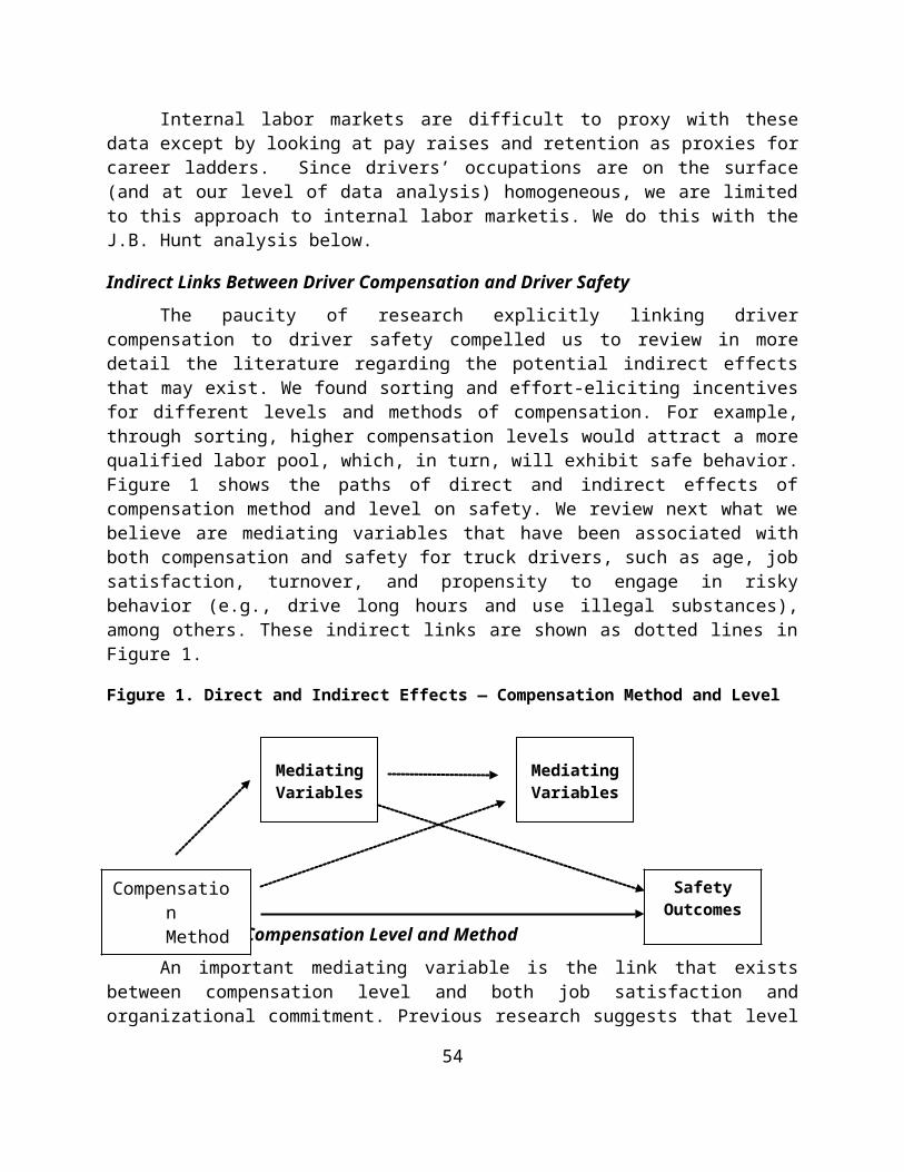
Figure 5: Labor Supply Curve for Over-the-Road Truck Drivers

54

Labor Supply Curve Estimation

The primary purpose of this section is to estimate the determinants of the number of weekly hours worked by drivers. Of particular interest is the relationship between mileage rates and hours of work. However, since it is reasonable to assume that hours might be determined in part by some of the same random components that influence mileage rates, it is not possible to estimate this relationship directly. It is therefore necessary to use a two-step procedure, first estimating the mileage rate for each driver, and then using the fitted values of the mileage rate to estimate the hours equation.

Each equation was estimated using ordinary least squares (OLS). The general form of the model can be written as:

Ratei = 1 + 2Xi2 + 3Xi3 + . . . KXiK + i

where Ratei is the mileage rate for the ith driver, the X’s represent characteristics of the driver and job that are relevant to determining the mileage rate, and the ’s are the parameters to be estimated. The term summarizes the random components and unobserved characteristics of the individual driver.

The variables used to estimate the mileage rate equation can be divided broadly into two groups. The first group of variables represents the human capital characteristics of the individual driver. These include experience, tenure, race and union status. The squares of experience and tenure are included to allow for a non-linear relationship between these variables and the mileage rate. In addition, the interaction of race and union status is included which would allow the union premium to differ by race. Finally, education and the previous driving record of the driver are also included as measures of the skill and performance levels of the individual drivers.

It would be expected that the mileage rate would be positively associated with experience and tenure, but a negative second order term would indicate that this premium is decreasing. Unionized and white workers might be expected to earn more. However, the interaction would be expected to be negative, since unions tend to equalize the wages of workers who otherwise might be expected to earn less. In this case, it would be expected that unions would raise the mileage rate of black drivers by more than that of white drivers. While in most occupations, a high school degree would be expected to raise the wage rate, this may not be true among truck drivers, since the formal education requirement of most jobs is rather low. Finally, those drivers with a previous moving violation might be expected to receive a lower mileage rate.

The second group of variables captures characteristics of the firm and job. It has been documented in other cases that large firms pay higher wages. Private carriage firms (versus for-hire firms) and firms that haul primarily dryboxes (versus refrigerator and tanker firms), might be expected to pay different mileage rates, but the direction of these differences cannot be predicted in advance. Drivers with longer dispatches might be expected to earn a lower mileage rate since they are able to spend a greater percentage of their time driving. Finally, the amount of unpaid time and paid time off are also included. However, the direction of these influences cannot be determined in advance. Firms that require a substantial amount of unpaid time for loading, waiting or other activities may or may not be compelled to compensate their drivers by

55

paying a higher mileage rate depending on other characteristics of the job. Similarly, it might be the case that more paid holidays and longer vacations are compensation for a lower mileage rate, or they could be complementary aspects of ‘good’ jobs that offer better compensation in all areas.

The data used in the study are summarized in Table 1. The sample consists of all full time drivers who are employees and paid by the mile. Owner operators and those drivers who are paid hourly are not included since it is difficult to make a valid comparison of their wages. The estimation is based on a sample of 233 drivers for whom complete information was available.

The average hours worked is 64.49 with a minimum of 25 and a maximum of 126. They are paid an average of .286 per mile with a range from .13 to .485. The average experience is 13.66 years and the average tenure is 3.46 years, and 83% of the drivers have a high school degree. A number of the variables in the study are categorical. Union members account for 8% of the sample, 86% are white, 25% have had a moving violation in the past year, while 33% work in a ‘medium’ sized firm, (between 100-500 workers) and 34% work in ‘large’ firms with over 500 workers. Other firm characteristics include 14% of the drivers working in the private carriage segment of the market, while 65% haul dryboxes.

The average miles per dispatch is 858 with a standard deviation of 619.75. Two variables of particular importance involve compensation for time spent in activities other than driving. The variable, “unpaid time” measures the number of minutes of unpaid time per mile driven. The average driver spend about .23 minutes in uncompensated activities per mile driven. Given the average of 858 miles per dispatch, this means that the typical run includes about 197 minutes of uncompensated time. At the other end of the spectrum, the typical driver receives 13.7 paid holiday, vacation and sick days per year, with a minimum of zero and a maximum of 35 days.

The last group of characteristics includes age, with an average of 42.18 years, and marital status, with 69% of the drivers married. The variable “other income” is the measure of total family income less the income earned from driving. This can include income earned by other family members, or by the driver in other occupations. The mean value is $31,978 with a standard deviation of $18,878. The final variables used in the study indicate that 22% of driving occurs at night (between the hours of midnight and 6:00 a.m.), and that 19% of the typical driver’s time is spent in non-driving activities. Finally, the typical driver last slept at home 8.46 days prior to the interview.

The results of the mileage rate equation are reported in Table 2. These show that the returns to tenure are statistically significant at the 5% level of significance, and the returns to experience are significant at the 10% level. However, the point estimates indicate that an additional year of tenure (and experience) increases the mileage rate by less than .005 per year. However, union members can be expected to earn almost $0.10 per mile more than non-union drivers, and this estimate is significant at a 1% level of significance. The returns to education and racial differences in compensation are not significant; neither is the interaction of race and union status, which indicates that the union premium is similar for all drivers, regardless of race.

The firm level characteristics offer a great deal of insight into differences in driver compensation. Workers in large firms are paid significantly more than those in smaller firms, while workers in private carriage firms earn less. In addition, workers with more paid time off also receive higher mileage rates, indicating that ‘good jobs’ reward workers not just by paying

56

higher wages, but with other forms of compensation as well. Finally, drivers with longer dispatches are paid less per mile than those with shorter dispatches.

In order to estimate the weekly hours equation, it is necessary to include variables in the mileage rate equation that do not determine hours of work. In this case, we hypothesize that experience and tenure will influence wages, but not hours. In addition, education, race, and firm size are also included in the wage equation, but are not used to determine hours worked. Finally, the size of the firm and the type of trailer are not included in the hours equation. The weekly hours equation can be written as:

Hoursi = 1 + 2*Wi + 3Wi2 + 4Zi4 + … KZiK + i

where Hoursi are the weekly hours of the ith driver, and Wi is the fitted wage of the ith

driver from the regression estimates described above. The Z’s represent characteristics of the driver and job that influence the number of hours worked, while i captures the random components of the hours worked not .included in the explanatory variables.

Both the fitted wage and its square are included in the regression. This allows the influence of the wage rate to decrease, and even allows for the possibility of a ‘backward bending’ supply curve where higher wages actually cause a decrease in hours worked. The other variables included in the regression are age (and it’s square), marital status and other income. Characteristics of the firm and job that might influence hours worked are also considered. These include the percentage of driving done at night, the percentage of time spent in non-driving activities, the amount of unpaid time, and paid days off. Union status, length of dispatch, private carriage and tenure are also included. Finally, the variable ‘last home’ is a measure of how long it has been since the driver has slept at home.

The results of the hours equation are reported in Table 3. The first thing to note is that weekly hours are not estimated as precisely as the mileage rate. One obvious reason for this is that the reported hours may be measured with error, relative to the explanatory variables. The weekly hours are reported for the most recent week. However, it is possible that the hours worked in any given week may over or under estimate the hours worked in a typical week. As long as these differences are not systematic, they do not bias the parameter estimates, but do make them less precise, which is reflected in the results.

Some results of note are that weekly hours tend to increase with age, until the driver is about 44.8 years old, at which point they decline. Married workers tend to work fewer hours, but this result is significant only at the 10% level of significance. Finally, it is necessary to interpret the results on non-driving time. The variable “unpaid time” measures the amount of unpaid time per mile driven. The estimate indicates that if a driver is not paid for his non-driving time, he tends to compensate by working longer hours. The variable non-driving time measures the percentage of time that a driver spends in activities other than driving. While the negative coefficient may seem surprising, in conjunction with unpaid time, the interpretation of this variable to measure the effect of non-driving time that is compensated, at least in part. Therefore, it is not surprising that drivers with more non-driving time that is paid may work fewer hours, while those who have more unpaid non-driving time may work more.

57

The results on mileage rate can be interpreted as follows. The fitted value of the mileage rate and its square show an overall positive influence of wages on hours, for most drivers. However, these estimates are only significant at the 10% level of significance. The positive relationship between mileage rates and hours continues until the mileage rate reaches about $0.313 per mile, at which point we estimate that further increases in the mileage rate lead to a decrease in hours. This relationship is described in Figure 5. Of particular note are the predictions of hours worked relative to the current hours of service regulations, which generally limit drivers to 60 hours per week. For low mileage rates, increasing the mileage rate leads to an increase in hours worked. The mean rate of $0.286 provides an estimate of about 62.5 hours worked per week, with an increase to almost 65 hours. However, after this point, further increases in the mileage rate lead to a decrease in hours. This can be explained by the idea that once drivers are paid a high enough rate and are already working long hours, further increases in the mileage rate are used to ‘buy’ more time off rather than purchase more goods and services. This also may be explained by joint decisions of drivers and firms at higher or lower rates of pay: firms that pay a high rate of pay may systematically prefer that their drivers obey the hours-of-service regulations, while firms that pay a low rate of pay may recognize that their drivers cannot make a living working no more hours than the regulations allow, and may encourage or coerce them to work more hours and drive more miles. The point estimates indicate that if the mileage rate were to increase to $0.37 per mile, drivers would reduce their weekly hours to be in compliance with the current regulations. At this rate, drivers are being compensated at a rate sufficient for them to be able to satisfy their income requirements without being induced to work in excess of those mandated by law.

58

Table 1: Summary Statistics

Variable Mean Standard Deviation

Minimum Maximum

Weekly Hours 64.49 18.11 25 126Mileage Rate .286 .055 .130 .485Experience 13.66 10.12 1.00 43.00Tenure 3.46 4.58 .083 30.00HS Degree .83 .37 0 1Union .08 .27 0 1White .86 .35 0 1Moving Violation .25 .43 0 1Medium Firm Size .33 .47 0 1Large Firm Size .34 .48 0 1Private Carriage .14 .34 0 1Drybox .65 .48 0 1Miles Per Dispatch 858.01 619.75 144.14 3500.00Unpaid Time per Mile .23 .40 3.00Paid Days Off 13.70 8.40 0 35.00Age 42.18 9.51 22.00 64.00Married .69 .46 0 1Other Income 31,978 18,878 0 85,000% Night Driving .22 .21 0 .75% Non-Driving .19 .17 0 .89Last Home 8.46 12.74 0 90.00N = 233

59

Table 2: Mileage Rate Equation

Variable Estimate Standard Error t-value

CONSTANT 0.241 0.016 14.727 ***Experience 0.002 0.001 1.939 *Experience2 -0.000041 0.000031 -1.338 Tenure 0.003 0.001 2.057 **Tenure2 -0.000106 0.000069 -1.529 HS Degree 0.000574 0.008 0.067Union 0.097 0.027 3.531 ***White 0.015 0.008 1.749 *Union x White 0.040 0.030 -1.332Prev Moving Violation 0.006 0.007 0.988Medium Firm 0.013 0.007 1.698 *Large Firm 0.026 0.008 3.324 ***Private Carriage -0.019 0.009 -2.024 **Drybox -0.008 0.006 -1.261Miles per Dispatch -0.00002 0.000005 -4.056 ***Unpaid Time -0.009 0.008 -1.194Paid Days Off 0.001 0.0004 2.080 **

* significant at .10** significant at .05*** significant at .01

Valid cases: 233 Dependent variable: Mileage RateR-squared: 0.385 Rbar-squared: 0.340Residual SS: 0.431 Std error of est: 0.045F(16,216): 8.457 Probability of F: 0.000

The R-squared can be used to test the overall significance of the regressions as follows:

F = [R2/(K-1)]/[(1-R2)/(n-K)] which has an F distribution with K-1 and n-K degrees of freedom, where K is the number of included regressors. In our example, the R-squared of .385 for the first equation (reported in Table 2) yields an F statistic of 8.457 which is significant beyond 1% and the .16 for the second equation (Table 3) yields a value of 2.852, which is also significant at less than .01.

In these models, both hours and mileage rates are determined simultaneously. Therefore, there is no obvious dependent and independent variable. It is common, if not ubiquitous for labor economists to put the wage rate on the y-axis and hours on the x-axis. This is very similar to basic supply and demand models that have price on the y axis ands quantity on the x-axis despite the fact that these models are often discussed in terms of Q = f(P).

60

Table 3: Weekly Hours Equation

Variable Standard Estimate Error t-valueConstant -119.328 65.559 -1.820 *Fitted Rate 785.677 446.722 1.758 *Fitted Rate2 -1252.969 756.186073 -1.656 *Age 3.124 0.992 3.147 ***Age2 -0.035 0.011 -3.056 ***Married -4.827 2.672 -1.806 *Other Income ($1000) 0.023 0.067 0.336% Night Driving 9.377 5.666 1.654 *% Non-Driving Time -21.803 8.913 -2.446 **Unpaid Time 11.066 3.864 2.86 ***Paid Days Off -0.064 0.196 -0.327Union 9.759 9.207 1.059Miles Per Dispatch 0.001 0.002 0.386Private Carriage -3.487 4.256 -0.819Tenure -0.362 0.300 -1.207Last Home -0.008 0.094 -0.090

Valid cases: 233 Dependent variable: Hours Per Week R-squared: 0.165 Rbar-squared: 0.107Residual SS: 63580.403 Std error of est: 17.117F(15,217): 2.852 Probability of F: 0.000

While mileage pay can be the cause of hours of service violations, it might also lead to unsafe practices even when the number of hours worked is not in violation of these rules. Mileage pay creates an incentive for drivers to travel as fast as possible, which may create safety problems due to speeding or driving to fast for existing weather conditions. In order to see if this is the case, we investigate the number of citations received by drivers.

Changing these compensation practices would reduce the incentive for drivers to violate the hours of service regulations. This would also be true for increases in compensation rates, as discussed above.

Firm Level Data

In order to obtain a complete understanding of these issues, a number of methodologies have been employed. The first of these is a firm level analysis of safety related outcomes by merging the Signpost, Form M and MCMIS data sets. In addition, we have made use of detailed data gathered from a large carrier by the University of Michigan Transportation Industry Program. As described above, the Signpost data set is a non-random sample of all TL firms operating in the U.S. The data set includes a wide range of information regarding driver compensation, including rates and type of pay, benefits and training practices. In addition, a description of whether and how drivers are compensated for waiting and unloading time is also included in this data set. In order to obtain a parsimonious description of how compensation practices influence safety outcomes, we focus on a selected subset of the variables included in

61

the Signpost data. To determine how pay levels influence driver behavior, we include the starting base pay as an explanatory variable. In addition, we use information regarding tenure increases in order to control for the rate of pay for a typical driver and turnover at the firm.

Since virtually all of the firms included in the data compensate their drivers by the mile rather than hourly, this variable does not address the issue of how the type of compensation might influence safety outcomes. An area of primary interest where the type of compensation does vary across firms is the treatment of waiting and unloading time. Some firms compensate their drivers by the hour for this work, while others pay a flat or piece rate. Finally a number of firms provide no compensation at all for this work. Since it is not possible to obtain an exact comparison of these varied compensation practices, we surveyed these carriers to determine exactly how drivers are paid for non-driving time and reduced this measure to an index of number of paid hours per mile driven.

For those firms who compensate their drivers hourly at a rate that is comparable to what they might earn on the road, there is little if any incentive to falsify their logbooks. For every hour they do not claim as unloading time, they are able to drive an additional hour, but this driving time does not increase their income, since they forfeit a similar amount by failing to log their loading time. If a firm compensates its drivers for unloading time either by the piece or at a flat rate, there is an incentive to declare some, but not all of the time spent unloading. It is necessary to declare a minimum amount of time in order to collect the payment, but any time included after this does not increase the income of the driver. Finally, for those firms that do not compensate their drivers at all, there is an incentive to completely ignore unloading time, since every hour of uncompensated unloading time could be spent driving. Therefore, we determine from the data which firm practices create incentives for drivers to declare all, some, or none of the unloading time. In this manner, we estimate how these firm policies influence driver behavior in specific areas. In particular, we can estimate whether drivers are more likely to work in excess of the hours allowed by law, and how this behavior influences safety outcomes.

A final variable of interest in the Signpost data is the average miles per trip for each firm. Since accidents may be more likely to occur after long spells of driving, it is important to take this into consideration. Driving for long periods is more likely to occur on longer trips, so this variable serves as a proxy for increased risk faced by drivers working for firms with longer routes.

To consider the effect of driver compensation on safety issues, it is necessary to control for other practices undertaken by the firm as well. Simply establishing a correlation between compensation practices and safety outcomes does not rule out the possibility that the true causal relationship regarding these outcomes is the result of some other aspect of firm behavior. In order to isolate the effect of compensation on safety outcomes, it is therefore necessary to consider all of these firm characteristics simultaneously.

One limitation of the Signpost data is that it does not include other pertinent aspects of the firm such as size or how long it has been in operation. Moses and Savage show that characteristics such as firm size and the type of freight typically hauled are significantly related to accident rates. In addition, they find that a number of questions related to safety audits and driver qualifications also are important (Moses and Savage 1994). The number of power units was obtained from the 1999 National Motor Carrier Directory, for 1997 fleet sizes. Larger firms,

62

and those with higher annual miles would be expected to have more accidents regardless of whether safety practices are emphasized by these firms. Taken together, the Signpost and other added data provide a broad picture of the operating practices of these firms as well as their compensation practices that will allow us to obtain a complete description of how these characteristics and practices influence safety.

Individual Level Survey Data

An alternative data set that allows us to investigate the effects of compensation on driver behavior is the UMTIP driver survey. This survey is a random sample of drivers passing through truck stops during 1997 and 1998-1999. In addition to providing a detailed description of firm characteristics, the survey also provides information regarding the compensation practices facing the drivers. There are several advantages to using the UMTIP sample in addition to the data described above. First, the UMTIP sample provides information about the actual practices of drivers, rather than those practices reported by the firm. While the firm may indeed adhere to these practices in general, it may not be the case that they always do so. The UMTIP survey asks questions not only about the current trip, but also about the most recently completed trip, the most recent month and the past year. This provides a description of not only the current conditions faced by the driver, but also about the typical conditions as well.

Another advantage of the UMTIP data is that it provides a wider range of safety related information. The drivers are asked whether they have received a violation or been in an accident over the past year. In addition, they are asked questions about the number of hours they have worked, the types and sizes of loads they have carried, and whether they have driven while tired. While these types of behavior are not themselves negative safety outcomes, they are known to be highly correlated with accidents and violations. In firm level data it is not possible to determine the extent to which drivers are forced to undertake unsafe practices, since the only information available is the actual number of accidents and violations. Therefore, the individual level data obtained from the UMTIP survey allows us not only to determine the extent to which these types of incidents have occurred, but also the extent to which drivers are placing themselves at risk.

Some explanatory variables in the UMTIP driver survey can be used to determine the safety related issues described above. The survey includes controls for firm level information, including the size and compensation levels of the firm. We also have information about the individual driver, including age and experience. Finally we have information regarding the type of work the driver has been doing during the current trip as well as the most recently completed trip and the past year. Taken together, these variables provide us with a detailed description of the conditions faced by drivers, and how these conditions influence safety related outcomes.

Quantitative Firm Case Study at the Individual Driver Level

We use UMTIP’s TL carrier data set to test driver behavior within the constraints imposed by using drivers of a single firm. Even though the firm is the data source, rather than a sample of its drivers, we have high confidence that the data provided reflects actual practices.

From the data collected, we have looked into the relationship between accident occurrence and driver characteristics, employment history, and driving activity. These include the association between crash likelihood and (a) prior moving violations; (b) prior truck driving

63

experience; (c) pay level; and (d) pay increases, after controlling for other demographic and driving activity information. Results appear below.

Estimation Techniques

The estimation for the individual drivers is based on cross-sectional data. The data are dichotomous, which means that limited dependent variable techniques, such as probit or logit analysis are appropriate. There is one aspect of the UMTIP data that would be problematic for the limited dependent variable techniques. The first of these is the likely presence of heteroskedasticity due to the cross-sectional nature of the data. A modification of White’s technique to correct for general heteroskedasticity is possible for limited dependent variable estimation as well, and will be employed.

The estimation for data from the TL firm case studies is based on panel data. This is because we observe drivers for 26 periods of time (months). The variable regarding accident involvement is dichotomous, which points to use of a duration model (also known as survival analysis or reliability analysis). However, it is important to note that the firm level data offers a wider range of modeling possibilities. First the number of accidents per firm is an ordered categorical variable rather then the typically dichotomous variable observed for individual drivers. This means that count models such as negative binomial models are appropriate for the firm level estimation. If two years of data are available, a form of differencing can be employed that will allow us to remove any unobservable firm level characteristics that are constant across the two periods. This is particularly useful for firm level data, where much of the performance of the firm might be attributable to idiosyncratic characteristics such as who heads the firm.

Because the individuals in the rich micro-data set are not randomly selected, the presence of unobserved heterogeneity is unsettling and will yield biased estimates in a duration model. We have accounted for unobserved heterogeneity (or “frailty”) by implementing a mixing distribution of the gaussian and gamma families where appropriate.

Taken together these proposed methodologies have allowed us to investigate the link between pay rates, driver behavior and safety related outcomes from a number of different points of view. The firm level data enables us to look at how the institutional behavior of the firm is related to accident rates. The individual data provided by the driver survey provides a more complete picture of how drivers react to the constraints placed on them by their working conditions, and how these responses are reflected in their safety performance.

64

VI. RESULTS

Pay Level and Method, Cross Sectional Analysis

Data

Data have been discussed previously, but the discussion is repeated here for convenience. The primary data source for the firm level study was The National Survey of Driver Wages published by Signpost, Inc. This is a quarterly survey of 198 truckload firms of various sizes. Represented are all major truckload carriers and a sample of medium sized and smaller carriers. These firms were chosen on the basis of the Commercial Carrier Journal (CCJ) list and other sources of top 100, second 100, and other truckload firms. Signpost also includes most of their own subscribers in the data, but there are many firms in the sample who are not subscribers, and if the carrier is small, it might be left out of the sample. Signpost was unable to provide an assessment of the randomness of the sample. However, the Signpost data were recently used for a compensation study conducted by the American Trucking Association’s Research Foundation and are considered by many to provide a reasonable approximation of driver pay for the industry. The data for the firms was obtained from the fourth quarter of 1998. Crashes are DOT recordable crashes during 1998.

One weakness in the signpost data is a lack of detailed information on non-driving time. Since this variable was of considerable interest, researchers from the University of Michigan Trucking Industry Program at the University of Michigan Institute of Labor and Industrial Relations conducted phone survey of the Signpost firms during the summer of 2000. This survey asked a detailed set of questions regarding the amount of time spent on activities other than driving, and whether and how this time was compensated. This information was used to compute the variable “unpaid time,” which is described below.

Results

The variables used in the study are summarized in Table 4. The variable of interest (the dependent variable) is the number of DOT reported crashes during 1998. The sample used in the analysis consists of firms with mileage-paid employee drivers which responded to the UMTIP survey of Signpost respondent firms. Of approximately 178 firms which paid their employee drivers by the mile, we received valid responses from 102 firms, representing a response rate of two-thirds. These firms had an average of about 64 crashes per firm. The average starting rate of pay for a driver with three years experience was 28.6 cents per mile, with a minimum of 23 cents and a maximum of 38 cents per mile. The variable “unpaid time” measures the number of hours of unpaid time per mile driven. This variable provides a measure of the amount of uncompensated time relative the paid time. The mean amount of unpaid time is 0.004 hours per mile driven. Since an average trip in this data set is 906 miles, this means that the average driver worked 3.624 hours of unpaid time per trip. We hypothesize that a high percentage of unpaid time provides incentives for drivers to increase the number of hours worked, which might be expected to increase the number of crashes.

65

Table 4: Summary Statistics

N = 102

VARIABLE MEAN STANDARD DEVIATION

MINIMUM MAXIMUM

CRASHES 63.87 101.20 1 660MILEAGE PAY $0.286 .026 .230 .380UNPAID TIME .004 .004 .870 E-4 .017RAISE $0.007 $0.005 $0.00 $0.040SAFETY BONUS .490 .502 0= No 1= YesPRODUCTION BONUS

.284 .453 0= No 1= Yes

HEALTH INS $166.84 69.803 $0 $368.30LIFE INS $15,505 10,991.00 $0 $52,000PAID TIME OFF $773.56 $302.27 $250 $2,000GOVERNOR SPEED .765 .426 0= No 1= YesMILES PER RUN 905.85 472.77 400 3,800MILES PER YEAR (MILLIONS)

127.53 238.88 1.5 1,106.0

FLAT BED .206 .406 0 1VAN .510 .502 0 1POWER UNITS 682.94 1035.8 24 7193

Definition of VariablesCrashes Number of DOT Reportable CrashesMileage Pay: $/MileUnpaid Time: Number of hours of unpaid time per mile driven in a typical runRaise: Average yearly increase in mileage paySafety Bonus: 1 if firm offers a safety bonus, zero otherwiseProduction Bonus 1 if firm offers a production bonus, zero otherwiseHealth Insurance Contribution of DRIVER to health plan, per monthLife Insurance Amortized value of company paid life insurance policyGovernor Speed 1 if firm uses a governor, zero otherwiseMiles per Run Number of miles driven in a typical runMiles Per Year Total number of miles driven by all drivers in the firmFlat Beds 1 if primary trailer type is a flat bed, zero otherwiseVans 1 if primary trailer type is a van, zero otherwisePower Units Number of power units owned and leased by the firm

The variable RAISE measures the typical yearly increase in the mileage rate for drivers in a firm, with a minimum of zero and a maximum of 4 cents per mile. About half of the firms provide a safety bonus and 28% offer production bonuses. The HEALTH INS variable measures the required monthly contribution of the driver to obtain company provided health insurance, while LIFE INS measures the amortized value of the available life insurance policy. The average

66

driver contribution to the health plan is about $167 per month with a minimum of zero and a maximum of $368. There is similar variation in the value of the life insurance policy, with some firms offering no insurance, and others offering policies with a value over $50,000. The variable PAID TIME OFF measures the value of the sum of vacation, holiday and sick pay. The average firm offers about $774 worth of paid time off per year, with a minimum of $250 and a maximum of $2,000.

The variable GOVERNOR SPEED is a dummy variable that indicates whether a firm restricts the speed of the trucks in its fleet, with about three quarters of the firms undertaking this practice. The average length of a run was 906 miles and the average firm drove about 128 million miles (average length of run in the Signpost set seems about 50% greater than averages in other data sets, suggesting a possible bias toward longer runs and therefore a downward bias in the measure of unpaid time – hours of unpaid work per mile driven). About 21% of the firms haul primarily flat beds while about 51% haul vans, with the remainder primarily hauling refrigerator loads. Due to a number of differences in the behavior of tanker firms, these were removed from the sample. Finally, the average firm had 693 power units, with a minimum of 24 and a maximum of over 7000.

Based on conventional economic theory, we expected that the compensation variables would be negatively related to crashes. Those firms that provide higher levels of remuneration should be able to select their drivers from a pool of more qualified workers. To the extent that safety is a desirable characteristic, fewer crashes would be expected from these firms. This would include not only direct payments, but benefits as well. Therefore, it would be expected that firms offering higher mileage pay, better raises, more lucrative life insurance and more paid time off would have fewer crashes. Unpaid time and health insurance would be expected to have negative coefficients because unpaid time represents time not paid for, and the health insurance variable is the amount contributed by the driver (and therefore a pay reduction). The 401K plans offered by firms were not included in the model. The primary reason for this is that the existence and level of these plans was not available for a large number of firms in the study. In addition, the tenure required for vesting in these plans is far longer than the typical driver could be expected to attain. Therefore, a more generous 401K plan would not necessarily influence the behavior of the drivers of that firm.

The expected signs of the coefficients on a safety bonus and governor speed would be negative, since they indicate at least a nominal interest in safety and the bonus would suggest a positive monetary reinforcement for safe performance. On the other hand, production bonuses might be expected to have a positive sign, since they may induce drivers to work longer hours or driver faster than they would otherwise, and might generally provide incentives to trade productivity for safety. While the effect of the length of a run may be ambiguous a priori, there might be some expectation that longer runs are safer. Shorter runs often are associated with more urban driving on congested roads, which might lead to higher crash rates. Finally, the number of power units and yearly miles reflect the size of the firm and exposure respectively, and would be expected to be positively related to crashes.

Since the number of crashes can take on the value of any non-negative integer, a negative binomial model was used to estimate the parameters of interest. While a Poisson regression might also be considered, the Poisson model suffers from the disadvantage of imposing the restriction that the variance of the dependent variable be equal to the mean. Failure of the data to

67

meet this restriction is referred to overdispersion. The appropriateness of the negative binomial model is indicated by the significance of the estimate of the overdispersion parameter.8

The results for the firm level model are reported in Table 5. Of primary interest are the variables related to compensation. The estimated affect of an increase in mileage pay is a significant reduction in the number of crashes. The most transparent interpretation of this result can be observed from estimating the elasticity. The estimated elasticity of -0.52 indicates that a 10% increase in mileage pay would be expected to reduce crashes by 5.2%. The amount of unpaid time is also significant, with a 10% increase resulting in 1% fewer crashes. Higher raises also reduce the number of crashes but this estimate is only significant at the 10% level of significance.9

8 The Poisson model is a restricted version of the negative binomial model. To see this, allow N to approach infinity, and P to approach zero in such a way that NP = , a finite constant. Then using l’hopitals rule, it is possible to show that the ln(P(X=k)) for the negative binomial is the same as the ln(P(X=k)) for the Poisson. In addition, this means that the mean and variance of the negative binomial. While the point estimates from the Poisson model are consistent even in the presence of overdispersion, the estimated standard errors are biased, which means that the t-statistics are not valid. However, the negative binomial model remedies this problem. The fact that the overdispersion parameter is significantly different from zero in the negative binomial model indicates that this is preferred over the Poisson, in this case.

9 Technical notes.Fourth-order term for “power units.” The higher order terms for the number of power units in the firm

level (Signpost) data were included for a number of reasons. Power units may be a proxy for firm size, but more accurately are a proxy for the number of employees, and there are other factors with regard to size that explain why the fourth order term might be necessary. A second order (squared) term would seem plausible since increasing the number of power units would not necessarily be expected to cause a proportionate increase in crashes. However, a residual analysis showed that when only a second order term was included, that the model severely overpredicted crashes for small firms and underpredicted them for large firms. While there is no direct theoretical reason for including the higher order terms, this was necessary to remedy the problem, as the fourth order term mathematically specifies the shape of the curve of the power unit variable, though the higher order variables are outside the range of the data. That is, it should be noted that even though the higher order terms allow for the possibility of the number of crashes declining with an increase in the number of power units, this does not turn out to be the case. Within the data reported in the sample, the equation estimates that crash rates always increase with the number of power units. Thus, within the relevant range of the data, the fourth order curve has the same shape as the second order curve, that is, increasing at a decreasing rate. However, the higher order terms are necessary to capture adequately the shape of the curve indicated by the data.

“Firm size” and “power units” measure slightly different things, so it is important not to generalize with respect to firm size (either in terms of revenue or employees) without more research. In the Signpost data, the dependent variable is the number of crashes in a one year period. You would expect these to increase as the size of the firm increases. The question is whether the increase is proportional, i.e. does doubling firm size lead to a less than doubling, a doubling, or more than doubling of crashes? The graph in Figure 6 shows that the increase in crashes is rapid as the number of power units increases for very small and very large firms, but less rapid for moderately sized firms. We might suggest the hypothesis that as small firms become larger, they can afford better safety precautions, such as better maintenance of trucks, but this advantage is lost as the firms become ‘too’ large. Overall, crashes do increase with firm size, but at a slower rate, so that doubling firm size leads to a less than doubling in the number of crashes.

These findings are consistent with the results that show that individual drivers working at large companies have lower crash probabilities. If doubling the number of drivers in the firm leads to a less than doubling of crash probabilities (see above), then the individual driver at the larger firm has a lower crash probability than an identical driver at a smaller firm.

The shape of fourth order power units curve appears in Figure 6. The maximum point (where it turns down) is at 6,580 power units. There are only two firms in this sample anywhere near this large, one with 5,878 and

68

Table 5: Negative Binomial Regression Results

Variable Estimate T-statistic ElasticityConstant 3.09 *** 12.80MILEAGE PAY -1.83 *** -2.68 -.52UNPAID TIME 24.63 *** 5.68 -.10RAISE -8.72 * -1.89 -.06SAFETY BONUS -0.10 *** -3.56 -.10PRODUCTION BONUS -0.05 -1.60 -.05HEALTH INSURANCE ($100) 0.05 ** 2.00 .08

another with 7,193. This means that for all but one firm, the model predicts an upward sloping relationship, and this would clearly be true even for this firm, if there where more large firms in the sample. The shape of the curve is as we hypothesized. It rises rapidly, and then slowly, and then rapidly again, suggesting that in the middle range, once firms obtain a sufficient minimum size, they get a handle on safety management, but they may tend to lose control if the firms become too large. While industry segment may be a confounding variable (and hence more research is needed), it appears that something is happening with large carriers and crash rates increase markedly.

Overdispersion Parameter. The two methods most commonly used to estimate models where the dependent variable is a non-negative integer are the exponential and negative binomial. The exponential is simpler, but requires that the mean and variance of the dependent variable are equal. Since this is a restriction that is not likely to be met, the exponential distribution is not often used. When the variance is not equal to the mean, this is referred to as “overdispersion.” The negative binomial model is an extension of the exponential that allows the variance to differ from the mean. This requires the estimation of an additional parameter, referred to as the “overdispersion parameter.” If this parameter has a value of zero, then the exponential distribution is appropriate. In the Signpost data, the estimate of the overdispersion parameter indicates that the parameter is not equal to zero, and therefore that the negative binomial model is preferred to the exponential.

Calculation of unpaid time. We calculated non-driving and unpaid non-driving time as follows:First, we identified the major ways that drivers spent non-driving time. These were:

Waiting for a LoadLoadingWaiting to UnloadUnloadingDropping and Hooking

These times were obtained for the ‘typical’ run. We then determined whether the drivers were paid for this timeNeverSometimes, or conditionallyAlways

The “never” and “always” were easy. We assigned one and zero to the time spent in the activity. For “sometimes”, it was too complicated to try to determine how often or how much the driver was paid, so we assigned 0.5.

We than multiplied these to obtain the amount of unpaid time per run. However, since the same amount of unpaid time represents a bigger loss to the driver for shorter runs, we divided this number by the number of miles per run, to obtain a relative measure of the amount of unpaid time per mile driven. The same method was done for this variable in the Signpost data as well as the driver survey.

Average length of trip. The Truckload Carriers Association’s (TCA) studies of both the dry van and refrigerated carriers estimate between 35 and 45 hours per week in non-driving labor time (“Just In Time To Wait” program of the TCA; research conducted by Martin Labbe Associates; “1999 Dry Van Drivers Survey” and “1999 Refrigerated Drivers Survey”). Their reports further indicate that dry van drivers average more than 500 miles per run and make 5 runs per week, which at 50 miles per hour would mean they drive at least 2500 miles (50 hours) plus work the additional 35 hours of non-driving labor. The Signpost data report an average trip of more than 900 miles, which is nearly twice that found by Labbe’s survey. While we suspect the latter is closer to the truth, we are forced to use the actual data we have. If the average trip length for the carriers in the Signpost set is actually much lower, we will have underestimated the pay effect for “unpaid time.” For this reason we believe our estimates are conservative.

69

LIFE INSURANCE ($1000) -0.04 *** -3.08 -.06PAID TIME OFF ($1000) -0.04 -0.61 -.03GOVERNOR SPEED -0.19 *** -6.14 -.19MILES PER RUN (thousands) -0.03 -0.53 -.03FLAT BEDS -0.24 *** -5.37 -.24VANS -0.03 -0.70 -.03LOG MILES (millions) 0.04 *** 2.80 .04POWER UNITS 0.004 *** 20.94 .77POWER UNITS2 -1.60 E-06 *** -8.33POWER UNITS3 2.97 E-10 *** 4.17POWER UNITS4 -1.78 E-14 ** -2.46OVERDISPERSION PARAMETER

0.12 *** 6.16

* significant at .10 level** significant at .05 level*** significant at .01 level

N = 102Log-likelihood: -454.996Restriced Log-likelihood: -4648.659Likelihood Ratio Statistic: -8387.326 Significance Level: 0.000Chi-Square Statistic 465.016 Significance Level: 0.000

Definition of VariablesMileage Pay: $/MileUnpaid Time Number of hours of unpaid time per mile driven in a typical runRaise Average yearly increase in mileage paySafety Bonus 1 if firm offers a safety bonus, zero otherwiseProduction Bonus 1 if firm offers a production bonus, zero otherwiseHealth Insurance Contribution of DRIVER to health planLife Insurance Amortized value of company paid life insurance policyGovernor Speed 1 if firm uses a governor, zero otherwiseMiles per Run Number of miles driven in a typical runFlat Beds 1 if primary trailer type is a flat bed, zero otherwiseVans 1 if primary trailer type is a van, zero otherwiseLog Miles Natural logarithm of number of miles driven per yearPower Units Number of power units owned and leased by the firm

Elasticity. Safety and production bonus, governor speed, flat beds, and vans are indicator (“dummy”) variables. For these variables, the elasticity is the percentage change in the number of crashes when the value of the dummy changes from 0 to 1. The elasticities were calculated as follows. A 0.01 change in the mileage rate reduces crashes by 11.09,% or 0.1109. The 0.01 change in the mileage rate represents a 0.01/0.3027 or 3.3% change in the mileage rate. The formula is %change in crashes/%change in mileage rate or 0.1109/0.033 or 3.36 for Table 8 For Table 9, it is 0.1007/0.033 or 3.05 for Table 10, it is 0.0973/0.033 or 2.92 and for Table 11 (the turnover model it is 0.052/0.033 or 1.58. The reader is cautioned to avoid confusion because the base pay is measured in cents per mile, and the coefficient represents the change for a 1 cent change in base pay, which is 3.3%, based on the average base pay of 30.27 cents per mile.

70

Figure 6: Predicted Crashes

Firms offering a safety bonus can expect to have about 10% fewer crashes, while the influence of production bonuses is not statistically significant. Although the estimated elasticities are quite small, firms requiring higher employee contributions to health insurance have more crashes, while those with more generous life insurance policies have fewer crashes. Finally, those firms that offer more paid time off have fewer crashes as well.

Turning to other characteristics of the firm, we estimate that firms that have governors on their trucks have 19% fewer crashes than those who do not. Firms that operate primarily flatbeds have about 24% fewer crashes, while those that operate vans do not appear to be different, on average from than firms that haul primarily refrigerated loads. Similarly, firms with longer average runs do not have different crash rates. The variable of log miles is significant, but surprisingly, a 10% increase in miles indicates only a 4% increase in crashes.

The estimated influence of increasing the number of power units requires explanation. The first estimated model included only the number of power units. However, the fit from this model was very poor. An investigation into the residuals showed that the model was severely over-predicting the crash rates of larger firms. This result indicated that a higher order term was necessary. However, since there was no theoretical basis for the necessary degree of non-linearity, higher order terms were included as long as they were significant at the 5% level of significance. The results indicate, as expected, that firms with more power units have more crashes, and that a 10% increase in the number of power units will result in 7.7% more crashes.

71

0

100

200

300

400

500

600

700

800

900

1000

1 1001 2001 3001 4001 5001 6001 7001

Power Units

The results described by the negative binomial model are almost uniformly consistent with those predicted. However, additional insight into the effects of compensation on crash rates can be obtained by considering the overall effect of these variables: mileage pay, unpaid time, pay raise, safety bonus, production bonus, health insurance, life insurance, and paid time off. The included variables account for a large part of the overall compensation package offered by most firms. Therefore, a 10% across the board increase in these variables would be consistent with about a 10% increase in compensation costs. If the effects of such an in increase on crashes are independent of each other, the effect of a 10% increase in compensation could be estimated by adding the individual estimated elasticities. These elasticities sum to –0.92, which means that a 10% increase in compensation would be estimated to cause an 9.2% decrease in crashes. 10

Pay Level and Safety: The Case of a Large Pay Raise

The truckload industry has long been characterized by low wages, along with the “driver shortage” much discussed in the media. We have hypothesized that these low wages have led to a safety problem on the highway. We sought to test this hypothesis by studying a single large truckload carrier, J.B. Hunt, which made a strategic decision in 1996 to increase pay by one-third.

The carrier’s goal was to increase both safety and productivity of drivers by paying an efficiency wage: a wage somewhat higher than that necessary to attract drivers at the margin. According to the firm, the new wage allowed them both to identify and hire drivers with the characteristics they desired. It also allowed them to terminate drivers who did not meet either safety or productivity standards. Our goal was to determine whether efficiency wages had the effect of increasing safety performance.

This wage increase gave us the opportunity to witness and test a social experiment. We attempted to distinguish between the sorting effect11, the selection effect12, and incentive effect13. We assume that a “good driver” is a safe and productive driver, and returns value to the firm and to the public. That is, it is in the firm’s interest to reduce cost (recruitment, selection, training, and casualty cost) while increasing revenue (increased productivity and greater reliability).

We model the influence of compensation on crash risk using a semi-parametric hazards approach. Building on prior safety research employing related methodologies (Jovanis and Chang 1989; Chang 1990; Mannering 1993), we allow the shape of the baseline hazard to be determined non-parametrically rather than imposing a particular distribution14. Furthermore, we allow the incorporation into the model of “unobserved heterogeneity,” referring to characteristics 10 We also examined truck out-of-service and driver out-of-service as possible dependent variables, and results where very weak. For “driver out-of-service none of the variables were significant. For “trucks out-of-service”, pay and life insurance were significant at 5% for lower crashes, but the overall model results were not significant. Reportable crashes were the most reliable proxy for safety outcomes in our research.11 From the firm’s perspective, the sorting effect is the effect on safety outcomes of those who stay at the firm (which we call “stayers”) when the firm upgrades its compensation package. From the labor market perspective, the sorting effect represents differential human capital available in the marketplace, and ranking of individuals by human capital and the labor market employment consequences of this ranking.12 The human resource management term for the firm’s hiring preferences given the greater range of choice provided by a higher compensation package.13 “Stayers” are those who remain with the firm when it upgrades the compensation package. These employees have incentives to perform at a higher level, and are willing to exert special attention in an effort to retain their jobs, which are more attractive due to the improved pay.

72

that differ across individuals but are not observable in the available data15. A compelling reason why it is important to consider a semiparametric baseline hazard and to account for unobserved characteristics is that failure to do so may lead to false inferences regarding the importance of compensation, operating conditions, and driver characteristics on likelihood of future crash involvement.

Our results suggest that the pay increase corresponded with a reduction in crashes by approximately 50%, along with a corresponding reduction in turnover of a similar scale. Hunt was able to hire an older, more married workforce (generally a proxy for stability) with more experience and superior unmeasured characteristics.16 The decline in turnover reduced crash risk attributable to unfamiliarity with the job and the trucks, and to pressure and stress associated with change.

We conducted a multivariate analysis using semi-parametric hazard modeling techniques discussed extensively by Meyer (1990). Specifically, we define Ti as a discrete random variable representing the duration of stay in a non-crash state for person i. Said differently, Ti is a variable at which the end of the non-crash spell occurs for person i. Durations are modeled as the distribution of transition probabilities between a non-crash state and a crash state (i.e., the probability of ending a spell at each time period). The calendar time is not the same for all drivers and therefore we measure duration on person-specific clocks that are each set to zero when we begin to observe each individual.

Suppose there are truck drivers i = 1,...,N, who each are in the non-crash state at time 0. The recorded duration for each driver i is the interval [ti -1, ti). Drivers also are recorded as either having a crash during the interval (contributing completed spell data) or as still remaining in the non-crash state (thus contributing right-censored spell data)17. The hazard probability hit , the 14 We do not assume a priori a parametric distribution for how crash hazards vary with time. While some researchers have specified an exponential distribution, we prefer not to impose such distribution on the data. Rather, by using dummy variables for each time period observed, we allow the data to show the underlying distribution of the baseline hazard. The result is a piece-wise linear baseline hazard function that is more general than imposing a given distribution.15 Although economists have theorized about the implications of human capital on performance, most aspects of human capital in actual labor markets are unobserved, as standard data sets include age, education or training, and perhaps experience as the only measures. We have found, for example, that educational attainment does not predict driver performance, suggesting that other factors explain performance (experience, job history, training, temperament, and other unmeasured factors). For an analytical examination of the issue of unobserved heterogeneity, or perhaps more particularly the heterogeneous unobserved human capital characteristics of individuals in the labor market, and firms the impact on unobserved worker heterogeneity on the economy, see Abowd, Kramarz and Margolis (1999).16 As we indicate below, we analyze variables Hunt happened to put into its administrative data set: age, gender, marital status, race, pay, mileage, season, number of dispatches, division within which driver is assigned, and experience (but only for the second year of the data set, since Hunt did not record experience initially as most drivers were inexperienced “students.” Most human capital characteristics, however, are not included in this data set.17 Censoring is an attribute of time-to-event or duration data. Broadly speaking, censoring occurs when a duration (time-to-crash, for example) for some subjects is known to have occurred during a certain interval, while the rest of durations (for other subjects, or for the same subject) are known exactly. In other words, for drivers in our Hunt data, we either know their exact time to a crash (because we observed them involved in a crash in month X) or we have a vague idea (because we observed them until a certain point, so at least we know that before that certain point they weren’t crash-involved, but they could be involved beyond that point. A classic example of censoring is the date we decided to stop collecting Hunt information (also called right censoring or type I censoring). Beyond that date, whatever observations we had may or may not be involved in a crash. They are censored observations. Another

73

probability of moving to a crash-state having survived until t in a non-crash state, can thus be expressed as

[1]

where Xit is a vector of covariates summarizing observed differences between individuals, which may vary with time. The conditional probability of a crash occurring given survival up to time Ti = t (i.e., censored cases) is

[2]

and

[3]

for non-censored cases.

Therefore, the likelihood for the entire group is

,[4]

where i = 1 for non-censored cases and 0 otherwise. The log-likelihood function is thus

.[5]

By defining an indicator variable, Jenkins (1995) rewrites the likelihood function in the form of a standard log-likelihood function for a binary dependent variable where the unit of analysis is the person-month as

example with the Hunt study is the hole in the data in the middle of the calendar time when we did not collect any information. For drivers that left that company during this period, we know it happened, but we don’t know when exactly. This is called “interval censoring.”

74

[6]

thereby allowing convenient estimation of these models with available statistical packages.

Hazard Rate

We need to identify an expression of the hazard rate for the particular crash process in order to specify fully the likelihood function. This, of course, has a substantial impact on the inferences made about the process. As expected, interpretation of the covariates varies according to hazard specification selected.

We use a complementary log-log specification for the hazard rate:

, [7]

where ' is a vector of parameters to be estimated and (t) is a function describing duration dependence18 in the hazard rate. This specification results in a model that is the discrete time counterpart of the continuous time proportional hazards model (Prentice 1978; Jenkins 1995). A proportional hazards specification refers to the influence of any covariate having a multiplicative effect on the baseline hazard function. Such specification has been used elsewhere in other safety research (see Jovanis and Chang 1989; Chang 1990; Mannering 1993).

We model the hazard rate’s duration dependence semiparametrically using time dummy variables for time periods during which drivers are observed. The underlying assumption is that the hazard is constant during the time period captured by each dummy variable. Thus, dummy variables provide information on how the baseline hazard rate increases or decrease across time periods thereby explicitly allowing for occurrences of periodic heterogeneity (Box-Steffensmeier 1997).

Incorporation of Unobserved Heterogeneity

Initially we assume that the population is homogenous with respect to the covariates Xit

that affect the duration distribution. This means that every person’s duration in the non-crash state will be a realization of a random variable from the same probability distribution. However this assumption can be violated with the current research design. Recruiters, for example, can hire individuals based on traits unobserved (to us) such as prior driving experience, character, or 18 Duration dependence can be also referred to as time dependence, a common characteristic of time-to-event studies. It means that the results can depend (positively or negatively) on how long the study has been observing subjects. Take the Hunt example. It is unfair to compare all drivers for whom we observed their 5th month of driving with drivers for whom we observed their 25th month of driving because the average driver whose 25th month we observed is probably quite different from the average driver for whom we observed a 5th month of driving. We expect the drivers in the 25th month to have more of the characteristics that lead them to stay longer, like higher age and higher experience, than those drivers present in the 5th month. In part this is why crash risk decreases the longer we observe drivers: drivers whom we observe for very long periods tend to be really good drivers, on average. That justifies our use of quasi-experimental tools (regression analysis) to attempt to account for such time dependence.

75

disposition. A practical consequence is that our sample may contain some degree of unobserved heterogeneity that often leads to hazard rates biased towards negative duration dependence (Heckman and Singer 1985).19

A solution to addressing the problem of heterogeneity, other than incorporating additional variables into the model, is to generalize the hazard rate specification to include an additive error-term i at the individual level with mean zero and uncorrelated with the X it vector. The error term for the sample is then assumed to follow a parametric distribution and by integrating it out of the likelihood function, model estimation is feasible (Jenkins, 1995). This means imposing a distribution, such as normal, lognormal, or gamma on failure-prone individuals and a different distribution for those less “vulnerable” (Lancaster, 1990). The problem is that neither theory nor data provides much guidance for imposing a specific distribution (Box-Steffensmeier, 1997). Instead of a specific heterogeneity distribution Heckman and Singer (1985) derive an nonparametric estimator. Kiefer (1988) however, suggests that Heckman’s estimator is sensitive to the selected parametric form of the hazard for the general model and to the explanatory variables selected. We therefore parameterize the heterogeneity term using a gamma distribution.

Data

We use demographic, operations, compensation, and crash data for unscheduled over-the-road drivers of a large U.S. truckload firm over a period of 26 months (Table 6). The data cover two periods of 13-consecutive months each, beginning in September 1995 and ending in March 1998. Accordingly, there are five months between October 1996 and February 1997 during which no data were collected and thus observations are treated as censored. The end of the first period coincides with the announcement of changes in the firm’s human resource practices designed to improve driver safety and reduce employee turnover. Of particular interest to this study are significant increases in driver per-mile compensation that took place at the beginning of the second period. On average, drivers observed during both time periods had their pay increased by 38% or 10 cents per mile driven. Other changes announced include the establishment of safety bonuses and a heightened emphasis on fulfilling drivers’ requests to get home within a given time frame.

The compensation and operations data gathered deserve additional explanation. For driver compensation, we use driver base pay, which is the per mile pay rate earned by drivers when first hired. Even though the firm provides other income to drivers such as safety and productivity bonuses, the vast majority of their income results from miles driven, and these data are not available in our data set. In addition, we use the percent pay increase per driver, which summarizes the percent pay raise announced on October 1996 and implemented on February 1997. Only drivers who were hired before the announcement and remained with the firm until the pay raise became effective had their pay increased.

In terms of operations data, average monthly miles driven is a measure of average productivity and thus captures average earnings up to the beginning of each month. In contrast, miles driven during a month summarizes each driver’s crash exposure. This information is

19 Heckman and Singer (1985) and Sancaster (1990) show that unobserved heterogeneity leads to a bias in the coefficients estimated in the model (including the estimates for the baseline hazard). Particularly, such heterogeneity results in coefficients that are higher than the true coefficients. It is labeled negative duration dependence because the bias leads to an artificial increase in crash risk (and thus lower duration in a non-crash state).

76

complemented with data summarized by the total number of monthly dispatches. All else held equal, a higher number of dispatches involves a higher likelihood of engaging in unpaid and unproductive waiting time and more pulling-in and out of conflict zones such as docks and urban areas. Finally, we also controlled for the possible seasonal effects of weather on crash risk. December through March were classified as winter months for this purpose. Table 6 provides descriptive statistics of key information summarized at the individual level. For variables that change with time, such as percent pay or miles driven, summary statistics at the individual level in Table 6 provide a skewed and incomplete picture.

Table 6. Descriptive statistics summarized at the individual level

Mean or Percentage

Standard Deviation

Min Max

Age (yrs.) 40.12 10.23 20 76Female 4%White 77%Non-married 52%Base pay (cents/mi) 30.27 6.73 16 48Percent pay increase 5% 12% 0 111%Tenure at firm with t = 0 (yrs.) 1.10 2.17 0 19.1Total miles driven during each month 7,500 3.19 4 23,863Total dispatches during each month 13.42 5.13 1 49Percent of driving during winter month 38%Percent individuals hired after pay raise 60%Note: Unit of analysis is individual drivers, independent of duration of observation.N: 11540

We observe a total of 11,540 individuals for at least one month of activity. As with the period with no data, a given month during which drivers had no activity is treated as a censored observation. Regarding the distribution of observed times, 50% of the drivers are observed 5 months or less, 75 percent are observed 11 months or less and only 5 percent of drivers are observed the full 26 months (their duration of employment at Hunt lasted at least the full 26 months of the study, plus the intervening months between before and after the wage increase). Furthermore, the average driver duration of employment for the group observed is 9.2 calendar months when censored observations are included, with a standard deviation of 8.7. These figures confirm the importance of understanding driver turnover in the truckload segment of the trucking industry in the U.S. Furthermore, they underscore the existence of at least two groups of drivers: one that engages in high turnover, often leaving the firm for jobs in other firms or occupations, and another that remains with firms for a longer term.

Only crashes involving $200 or more of actual or estimated damages are included in the analysis. A stylized analysis shows that the first period had 1,535 crashes (which occurred during 3.6% of person-months) while the second period had 783 crashes (1.6% of person-months) reported. In individual terms, 18.4% of drivers during the first period and 10.6% of drivers during the second period reported crashes. Finally, the probability of transitioning to a crash state during a month, given that the driver is in a non-crash state the month before, is 3.5% before the wage change and 1.5% after the wage increase. Interestingly, the probability of remaining in a

77

crash state for any driver is 5.9% during the first period and 2.2% for the second period, which suggests that the first months of employment are critical for repeat crashes. 20

Demographic changes were notable between the two periods: the second period shows an increase in average driver age, and in the percent of males, whites, and married drivers (Table 7). These increases can occur if higher quality drivers are being attracted by the pay raise and the underlying time dependence of the data causes changes in unmeasured driver characteristics consistent with safety, and where these indicators proxy unmeasured characteristics of these drivers which are associated with lower crash rates. One poorly-measured variable, for example is experience: Hunt entered experience information in the database only during the second period21. Other increases in the number of miles driven and the number of dispatches per month per driver also are detected. The decrease in the standard deviation of miles and dispatches suggests that the work was more evenly assigned among drivers during the second period (between rows in Table 7) and for each driver over time (within rows in Table 7).

Table 7: Descriptive statistics summarized at the individual level before and after pay raise

09/95 to 09/96 Period 03/97 to 03/98 Period

(N = 42,295person-months)

(N = 50,233person-months)

Mean Standard Dev. Mean Standard Dev.

Age at t = 0 (yrs.) 38.0 10.0 41.6 9.6% Female 3.6 18.6 2.0 13.9% White 72.9 44.4 78.2 41.3

% Nonmarried 53.6 49.9 43.8 49.6

Base pay (cents/mile) 26.2 4.3 33.0 6.06% Pay raised 0.0 0.0 10.0 4.0

Miles driven per month per driver overall 9,155 4,150 9,170 3,086

between 3,625 3,005

within 2,731 2,300Dispatches per month per driver overall 15.6 6.6 16.2 5.7

between 5.7 5.0within 4.9 4.4

Note: Unit of analysis is person-months, which depends on length of time individual is observed (female probability of turnover is 26% higher than male turnover, ceteris paribus).

20 Remaining in a crash state over two months means having at least one crash for two consecutive months.21 Previous unpublished research by Belzer has suggested that recruiters look for a bundle of characteristics, including the vague attribution of “character,” but the Hunt data set does not include such variables as previous employment stability or quality of previous employment, which might provide evidence of other unmeasured characteristics that might be explaining outcomes more explicitly.

78

Crash modeling

An illustration of how crashes, censoring, and time are associated is provided by the empirical hazard of crash involvement. The empirical hazard is the fraction of drivers ongoing at the start of a period that are involved in a crash during that period (Figure 7). As months observed increases, the pool of drivers that can crash decreases because a low number of drivers are observed for long time periods. Figure 7 suggests that the empirical hazard in several periods (15,20, and 2822) appears to be noticeably higher than in surrounding periods. A high hazard in the second month is probably due to drivers' inexperience. During the first month, drivers have a trainer with them at all times, whereas the second month of activity is when drivers begin driving alone. The spike at month 15 is roughly coincident with the highest number of censored observations, those taking place in the interregnum between the two periods of data. These censored observations correspond to individuals that were not observed during the time break but that were observed again later in time. If these censored cases were randomly selected, the spike would be a cause for concern. However, because these censored cases correspond to individuals that were with the firm at time zero and that are safer than other non-censored drivers, we can expect the empirical hazard to be higher for this time period than at other nearby time periods.

Figure 7: Kaplan-Meier Empirical Crash HazardThis is the empirical crash hazard, not accounting for possible underlying causes. It

suggests a declining crash hazard the longer we observed an individual. Is this finding a result of observing for longer time drivers that have certain characteristics, such as high tenure at firm, that lead them to be safer? It may also be that there is some true negative duration dependence –the longer a driver is observed, the safer he or she is. We explore the causal underpinnings using 22 The apparent spike in period two actually is the first complete month of observation, as drivers may have entered anytime during the first month.

79

0

0.01

0.02

0.03

0.04

0.05

1 3 5 7 9 11 13 15 17 19 21 23 25 27 29

Months observed

Cras

h Ri

sk

hazard 95% confidence bandN = 92528

the discrete time counterpart of the continuous proportional hazards model as proposed discussed above.

It is important to note that there can be conceptual difficulties because drivers are selected to work for this firm based on observed and unobserved characteristics. Given this stock-sampling design and the subsequent monthly follow-up, the variance of heterogeneity estimated applies to the sample but not the population and therefore the sample variance can be biased because of the unobserved selection that occurs.

More importantly, Figure 7 suggests that the longer drivers remain with the firm (and thus the longer we observe them in the data), the less likely they are to be involved in a crash. However, several aspects of Figure 7 point to the need for the duration modeling methodology suggested in the previous section. The Kaplan-Meier hazard assumes homogeneity in the sample, but we expect that the characteristics causing a lower hazard (observed or unobserved) are more concentrated among the remaining individuals the longer we observe them. For example, the remaining drivers are likely to be disproportionately older and perhaps better paid. This sorting effect masks underlying changes in the hazard and thus can affect the duration dependence of crash risk. Additionally, spikes in periods 20 and 28 have not been fully explained. We turn therefore to duration models’ results.

Crash Model Estimation Results and Discussion

We report estimates from the Prentice-Gloeckler (1978) model incorporating a gaussian mixture distribution to summarize unobserved individual heterogeneity as proposed by Meyer (1990). This model was preferred to those with no heterogeneity parameters (results not shown). Similarly, in the interest of parsimony, we include a total of 15 dummy variables (one for every two months) for estimating the baseline hazard semi-parametrically. We also select the period between 0 and 2 months as the base category.

Additionally, even though there is no compelling reason to support specifying proportional hazards vis-à-vis non-proportional hazards, all model specifications assume proportionality. We test this assumption by interacting each time invariant explanatory variable with a time variable measuring the length of spell. This test is performed by re-estimating the models with an additional covariate such that , where Xi is an explanatory variable already in the model and f (t) is a particular functional spell length distribution. The subscript for time has been dropped because by definition Xi does not vary with time. A test of the hypothesis that the coefficient for Xm = 0 is a test of the proportional hazards assumption for Xi. As a result of these tests, three terms are suspect of violating the proportionality assumption (AGE, BASEPAY, and WINTER) and thus time interactions with each are included in the model. The behavioral meaning of these interactions is not simple. In the case of driving season, for example, we expect the influence of driving in winter on crash risk to vary over time as a result of accrued driving experience.

80

Table 8 Driver Discrete Time Proportional Crash Hazards Model with Gaussian-Distributed Unobserved Heterogeneity

Crash Event = 1 Coeff. Z-statistic E-form % change in crash rate per unit change in variable

Age -0.089 *** -14.78 0.91 -8.54%Age2 0.002 *** 14.34 1.00 0.21%Female -0.186 -1.51 0.83 -16.95%White -0.543 *** -12.62 0.58 -41.93%Nonmarried -0.095 ** -2.39 0.91 -9.10%Base pay (cents/mile) -0.118 *** -17.08 0.89 -11.09%Percent pay increase -0.006 *** -2.61 1.00 -0.60%Average miles up to given month (000s) 0.014 1.39 1.01 1.40%Monthly miles driven during month (000s) -0.093 *** -8.23 0.91 -8.92%Dispatches -0.002 -0.36 1.00 -0.20%Tenure (years) -0.176 *** -5.88 0.84 -16.11%Tenure2 0.013 *** 4.93 1.01 1.29%Winter -0.142 ** -2.26 0.87 -13.25%Hired after pay raise 0.129 1.38 1.14 13.82%Age by time 0.001 ** 2.01 1.00 0.07%Base pay by time 0.004 *** 4.65 1.00 0.42%Winter by time 0.003 0.37 1.00 0.29%sigma_u 0.399 Rho 0.137*** Significant at a 99% confidence level** Significant at a 95% confidence level* Significant at a 90% confidence level

Log Likelihood = -10411.346Likelihood ratio test of gamma unobserved heterogeneity (rho = 0): 7.65; P = 0.003Number of driver-months = 92,528 Number of drivers = 11,540

The two variables associated with driver compensation, “basepay” and “percent pay increase,” have the hypothesized negative sign and are statistically significant. The coefficient estimates suggest that for every additional cent per mile paid when hired, crash risk for drivers decreases 11 percent. At the mean rate of pay (30.27 cents/mile – see Table 6) this translates into an elasticity of -3.4.23 Because driving experience prior to hire is missing, the pay level coefficient can be biased (if individuals who are paid more have more experience). The implications of this result are explored in more detail below. Furthermore, interactions between total months observed (time) and three other variables (age, base pay and winter) are included in the model because the variables violate the assumption of hazard’s proportionality. For pay this means that the longer a driver is observed, the lower the crash risk, although the effect is small relative to other effects estimated.

Similarly, a ten percent raise in driver pay is associated with six percent lower crash risk, all things held equal. Because only drivers spanning both time periods were subject to a pay 23 The reported coefficients are marginal effects. From these estimated marginal effects, the elasticities are derived by determining the percent change in the hazard (1-exp(estimated coefficient for variable X1)) vis-à-vis the percent change implicit by a unit change in variable X1.

81

raise, this parameter captures simultaneously the incentive effect of higher pay with the sorting effect attributed to unobserved characteristics having negative duration dependence of crash risk, and the sorting effect is the larger of the two. Thus, the pay increase variable captures not only the pay increase faced by drivers but also a self-selection effect related to who received a pay raise: drivers who are more prone to remaining employed with the firm than those who are prone to leaving the firm. As such, this coefficient should be interpreted with caution, as evidenced below.24

Figure 8 shows an estimate of how the probability of crashes (y-axis) changes with different levels of pay rate (x-axis). All other variables are held constant at their means. The graph is an estimate of the probability because the original equation estimated incorporates a normally-distributed unobserved heterogeneity term for each individual. For the purposes of producing Figure 8, the unobserved heterogeneity for each individual was assumed to be zero. For additional illustration, this figure includes the shape of the curve for two levels of driver tenure at the firm, 0 and 5 years. One must recall that we would not expect the effect to be linear; accordingly, the estimated line is curved.

By normalizing changes in crash probability and changes in pay depicted in Figure 8, one can estimate point elasticities. The short straight double line below the curve is the slope of the crash probability curve at the mean pay of 30.27 cents per mile. The overall slope of the line decreases as pay increases, as it should, because marginal effects of increased pay have a lower effect the higher we raise the pay rate, so we get a great deal of safety effect at the lower pay rates and we would expect the effect to flatten out at pay rates approaching the National Master Freight Agreement scale of approximately 50 cents per mile (which are not observed in this data set).

A unit increase in pay rate from 30.27 to 31.27 cents per mile, normalized by the base units, is a percentage increase of 3.33%. This pay increase lowers crash probability as depicted by the y-axis from about 0.0289 to 0.0257. In percentage terms, this decrease in crash risk is 10.7%. Summarizing in percentage terms, an increase of 3.3% in pay rate, evaluated at its mean and holding other variables at their means except for tenure which is held at zero, is associated with a decrease in crash risk of 10.7%. The point elasticity (ratio between 10.7 and 3.3) is therefore 3.21. This estimate differs slightly from the estimate reported from Table 8 for two reasons. First, Table 8 incorporates a normal mixing distribution. Second, the elasticity estimates derived from Table 8 hold all variables at their means. Since the mean driver tenure is 1.1 years (not zero) a slightly different estimate should be expected. See Appendix A for further graphs of these effects, controlling for different variables.

24 The sorting (or selection) effect stems both from decisions by the firm and individual decisions. The sorting effect results from the fact that individuals observed for 30 time periods are inherently safer than individuals observed only for a few months. The latter are observed for a few months because they are unsafe (and they or the firm terminate their employment), or they have low human capital and are unreliable or unproductive, or they simply decide to leave the firm or the industry. So the variable captures the incentive effect and this sorting issue. Both effects are expected to decrease crash risk. Insofar as we are interested in the incentive effect only, then the coefficient estimated is biased downwards (because sorting is confounded with selection). If, as we believe, most of the effect results from sorting, the effect is accurately estimated.

82

Figure 8: Elasticity of Crash Probabilities by Pay Rate and TenureMaking an efficiency wage argument, it may be that a driver’s base pay reflects

unmeasured characteristics – in addition to the demographic characteristics accounted for in this study – which explains his or her superior safety performance and productivity. Thus, “base pay” is the largest component of compensation and thus has the greatest impact on crash risk, but can also explain the presence of “good driver” characteristics that reduce crash risk (unobserved to us with this data set but observable to recruiters). This is particularly important if we recognize the potential role of driver experience on crash risk. Unfortunately, each individual’s prior driving

experience is only available for a subset of drivers, those hired after the pay raise became effective. The correlation between months of experience and base pay for the subset of individuals having the data available is relatively low, however (r=0.45). We further clarify the effect of experience on crash risk by estimating a model containing all independent variables used thus far in addition to months of experience for the subset of our data containing the required information (Table 9). The results confirm that higher base pay, independent of driver experience, is associated with lower crash risk. However, the results show that the percent increase becomes insignificant, suggesting that it was a acting as a proxy for months of experience.

In addition to compensation issues, there are two other variables related to human resources included in the model. First is the influence of tenure with the firm on crash risk. We find that for every additional year of tenure with the firm (TENURE), drivers are 16 percent less likely to have a crash, all else held equal. The squared tenure term is significant, suggesting that its effect on crash risk lessens as tenure with firm increases. Drivers with seven years of employment with J.B. Hunt face the lowest crash risk, whereas drivers with 13 years of tenure with the firm have a similar risk than drivers recently hired.

The second human resources variable of interest, AFTER, measures the selection effect of higher wages on the quality of new hires beyond what is captured by the observable

83

Predicted crash probability by pay rate and tenure

0.00

0.02

0.04

0.06

0.08

0.10

0.12

0.14

17 19 21 23 25 27 29 31 33 35 37Pay rate (cents/mile)

Pre

dict

ed P

roba

bilit

y of

Cra

sh

Haz

ard

0 years 5 years

characteristics included in this study. It is coded as one for drivers hired after the pay increase was announced and zero otherwise. Holding constant all other variables, the parameter estimate unexpectedly indicates that drivers hired after the pay raise announcement are as likely to be involved in a crash as drivers hired before the announcement. The sign and significance of the estimate has several competing explanations. One is that the model already accounts for the driver characteristics relevant to lower crash risks, such as age, exposure and base pay. The summary statistics of drivers before and after the wage increase (Table 7, above) are supportive of this interpretation. Further examination of the data suggests that drivers who were hired during the period after the raise were less experienced than the retained drivers who had been hired before the raise (perhaps as inexperienced drivers) and had gained their experience during their employment with Hunt. This explanation is consistent with the results obtained for total months of experience.

With respect to driver characteristics, the existing safety literature has emphasized a non-linear association between truck driver age and crash risk. Young truck drivers, particularly those under 25 years of age, tend to be over-involved in careless driving, traffic violations and crashes (Walton 1999; Blower 1996; Campbell 1991) Other research suggests that older drivers are more likely to fall asleep at the wheel (McCartt 2000) and may exhibit deficits in driving ability that are reflected in higher crash risk (Brock, 1996).

Our results show that driver risk decreases with age until the driver reaches 41 years of age, when the effect changes direction. We attempted other functional specifications of driver age – such as the inclusion of a cubed term for AGE, but results are not significantly different from those in Table 8. We estimate that a driver that is 20 years old has the same crash risk as a driver 62 years of age, all other characteristics held equal. Even though this result is consistent with the literature in the field, the drivers under study are not likely to be representative of the population of truck drivers, which may also explain differences with the existing literature. White individuals have a crash likelihood that is almost less than half the crash likelihood of individuals of other races and unmarried individuals appear to be safer than married ones. Finally, we detected no consistent crash risk differences by gender.

Two of exposure measures are statistically significant. First, and contrary to preliminary expectations, as the number of miles driven increases crash risk decreases. For every additional 1,000-miles driven during the observed month, crash risk decreases individually by 8.9 percent, all else held equal. This means that a one percent increase in miles driven is related to a 0.8 percent decrease in crash risk. Because higher miles means more use of divided, interstate roads this result is consistent with other research suggesting that local and regional roads are riskier than interstate highways. Second, driving during a winter month is associated with a 13.3 percent lower crash risk. Because private vehicle traffic decreases during winter months we interpret this result as supportive of the hypothesis suggesting that an important cause of truck crashes is related to behavior of drivers of private vehicles. Finally, the number of dispatches is not statistically significant despite having the expected sign.

84

Figure 9: Crash Risk and Age

Figure 10: Crash Risk and Tenure

The sigma_u coefficient reported in Tables 7 and 8 is the standard deviation of the heterogeneity variance. The reported rho is the ratio of the heterogeneity variance to one plus the heterogeneity variance. A likelihood ratio test of the null hypothesis that rho is zero can be rejected (p=0.003) and therefore unobserved heterogeneity or ”frailty” is important.

For the baseline hazard estimated using the time dummies described before, the following figure shows that after controlling for all other effects, the crash hazard continues, thereby suggesting negative duration dependence that goes beyond what is captured by the independent

85

variables. The analysis in the next page suggests that months of experience prior to hire is a key contributor to the duration dependence detected here.

Figure 11: Negative Duration Dependence and the Role of Experience

All results are as expected for every other variable, except AFTER where the results suggest that people hired after the pay raise are less safe than those hired before the pay raise. We have addressed this problem and have a compelling explanation for it: the omitted variable of driving experience. When hired, AFTER drivers tend to have somewhat more driving experience than BEFORE drivers (when hired). When the experience at the firm is counted as driving experience, however, the effect is reversed: BEFORE drivers tend to have higher overall experience. Because we do not have driving experience for everyone (only for those who stayed with the firm during the pay raise and for those hired AFTER the pay raise), we cannot control for experience in the global model.

To examine the relationship between months of experience prior to hire and crash risk, we estimated the model described above for a subset of the data for which this information was available. As a result, only drivers present after the pay raise (5,897 drivers) are included in this sub-model. The coefficients estimated (Table 9) show that a nonlinear relationship between total driving experience (defined as experience prior to hire + tenure at the firm + time observed) and crash risk.

86

Estimated Semi-parametric Baseline Hazard

Table 9 Driver Discrete Time Proportional Crash Hazards Model with Gaussian-Distributed Unobserved Heterogeneity –Months of Experience Subset(N = 52,393 driver-months; n = 5,897 drivers)

Crash Event = 1 Coeff. Z-statistic E-form % change in crash rate per unit change in variable

Age -0.100 *** -11.94 0.90 -9.52%Age2 0.002 *** 10.60 1.00 0.22%Female -0.232 -1.10 0.79 -20.69%White -0.471 *** -8.03 0.62 -37.56%Nonmarried -0.154 *** -2.78 0.86 -14.31%Base pay (cents/mile) -0.106 *** -11.70 0.90 -10.07%Percent pay increase 0.000 0.02 1.00 0.00%Average miles up to given month (000s) 0.032 ** 2.23 1.03 3.24%Monthly miles driven during month (000s) -0.111 *** -7.13 0.89 -10.51%Dispatches 0.003 0.36 1.00 0.26%Winter -0.213 ** -2.10 0.81 -19.16%Hired after pay raise 0.491 *** 4.78 1.63 63.44%Total experience (yrs) -0.049 *** -3.03 0.05 -95.1%Total experience2 0.001 ** 2.41 1.00 0.1%Age by time 0.001 ** 2.48 1.00 0.11%Base pay by time 0.006 *** 4.70 1.01 0.58%Winter by time 0.029 ** 2.36 1.03 2.98%sigma_u 0.399Rho 0.137Log likelihood = -5,478.65

Figure 12: Effect of total experience on crash risk87

The three main differences between the model estimated for the subset of drivers having months of experience information and the model with all drivers are:

1. Percent pay increase is not statistically significant, which is expected since this only includes drivers hired after the pay increase.

2. The dummy for individuals hired after the pay raise is positive and significant, suggesting that individuals hired after the pay increase have higher crash risk than individuals that benefited from the pay raise, all other things held equal. An important distinction should be made in understanding why this coefficient becomes significant with this subset of the data. For the data in Table 8, individuals hired after the pay raise are being compared to the heterogeneous group of individuals hired before the pay raise. The latter is composed of individuals who stay with the firm and get a pay raise, and those who leave the firm before the pay raise is in effect. As such, it is not unexpected to find that the dummy variable for the after group in Table 8 is not significant. In Table 9, the group is being compared solely against those getting the pay raise, who tend to be safer not only in terms of human capital, but also due to the sorting effect explained earlier.

3. The baseline hazard does not exhibit negative duration dependence. Driving experience appears to account for the duration dependence detected in the previous model.

Finally, we explore the association between prior moving violations and crash risk using only those observations for which the data are available. This model contains the largest number of variables of all models estimated. A total of 3,555 drivers (20,212 driver-months) are used in this estimation. The results suggest that having prior moving violations (coded as 0 = no, 1 = yes) is associated with a 20.4% lower crash risk. The reasons for such an effect are a matter of further empirical exploration. Many competing explanations exist, such as the behavioral effect that citations for moving violations may have on drivers. Most coefficients estimated for this model (Table 10) remain similar to results presented previously except for:

1. As with the months of experience model, percent pay increase remains statistically insignificant. This is mostly due to the presence of experience in this model.

2. Months of experience and its square become statistically insignificant.

3. The baseline hazard again exhibits negative duration dependence. See footnote 14 for a definition of duration dependence.

88

Table 10: Driver Discrete Time Proportional Crash Hazards Model with Gaussian-Distributed Unobserved Heterogeneity –Months of Experience AND Moving Violations Subsets(N = 20,212 driver-months; n = 3555 drivers)

Crash Event = 1 Coeff. Z-statistic E-form % change in crash rate per unit change in variable

Age -0.098 *** -8.73 0.91 -9.37%Age2 0.002 *** 8.53 1.02 0.23%Female -0.117 -0.44 0.89 -11.05%White -0.545 *** -6.46 0.58 -42.04%Nonmarried 0.040 0.5 1.04 4.07%Base pay (cents/mile) -0.102 *** -8.45 0.90 -9.73%Percent pay increase -0.002 -0.42 1.00 -0.17%Average miles up to given month (000s) 0.021 0.88 1.02 2.09%Monthly miles driven during month (000s) -0.164 *** -6.44 0.85 -15.09%Dispatches 0.029 ** 2.39 1.03 2.97%Winter -0.314 ** -2.16 0.73 -26.96%Hired after pay raise 0.310 ** 2.18 1.36 36.38%Total experience (yrs) -0.008 -0.33 0.99 -0.83%Total experience2 0.000 -0.24 1.00 -0.02%Prior moving violations -0.228 ** -2.41 0.80 -20.40%Age by time 0.001 1.39 1.00 0.11%Base pay by time 0.006 *** 3.41 1.01 0.63%Winter by time 0.049 ** 2.2 1.05 4.97%sigma_u 0.001rho 0.000Log likelihood = -2485.33

TL Case Study: Turnover Analysis

The safety analysis above shows that turnover represents an important indicator of crash risk. While tenure is not a straight line, for the first six months truck driver tenure represents a distinct predictor of driver crash probability. We therefore address the issue of turnover directly. What predicts driver turnover?

89

Figure 13: Raw Turnover RiskWithout controlling for other factors, we see that driver turnover decreases monotonically

in a rather linear fashion. For additional interpretation of this turnover hazard, please see the comments above regarding the interpretation of the empirical hazard curve for crashes.

Table 11: Driver Discrete Time Proportional Turnover Hazards Model with Gaussian-Distributed Unobserved Heterogeneity

Event: Leave the firm = 1 Coeff. Z-statistic

Eform Change in turnover rateper unit change in variable

Age -0.020 *** -4.90 0.98 -1.9%Age 2 0.000 *** 4.02 1.00 0.04%Female 0.232 *** 3.78 1.26 26.1%White 0.151 *** 5.08 1.16 16.3%Nonmarried 0.089 *** 3.44 1.09 9.3%Base pay (cents/mile) -0.053 *** -14.81 0.95 -5.2%Percent increase -0.002 *** -12.26 1.00 -0.2%Average miles up to given month (000s) 0.065 *** 12.22 1.07 6.7%Dispatches -0.181 *** -68.03 0.83 -16.6%Tenure (years) -0.367 *** -16.50 0.69 -30.7%Tenure 2 0.019 *** 8.78 1.02 1.9%Peak activity period (Sept-Nov.) 0.396 *** 13.02 1.49 48.6%Hired after pay raise -0.284 *** -4.92 0.75 -24.8%sigma_u 0.001rho 0.000*** Significant at a 99% confidence level** Significant at a 95% confidence level* Significant at a 90% confidence level

Log likelihood = -16510.36Likelihood ratio test of gamma unobserved heterogeneity (rho = 0): 0.00; P = 1.00

90

Kaplan-Meier Empirical Turnover Hazard

Coefficients estimated, as shown in Table 11, suggest that driver turnover risk decreases monotonically with age until age 43 and then begins to increase (for graphical depiction see Figure 14 below). We estimate that a driver who is 25 years old has the same turnover probability as a driver 65 years of age, all other characteristics held equal. If age is viewed as proxy for driving experience, the decrease in crash risk associated with young age can be interpreted as supportive of the influence of wage growth on individual decisions to leave the firm. Because prior driving experience is key for determining pay level, young individuals with little or no experience face a steeper wage growth curve than an individual with some work experience.

Figure 14: Turnover Probability by Driver AgeConsistent with prior research, females are more likely to leave the trucking firm than

males. This may be related to the incompatible demands between domestic responsibilities and the lifestyle afforded by unscheduled truckload driving. Similarly, the coefficients estimated suggest that married individuals are less likely to leave the company than non-married individuals. Finally, individuals self-identified as white in the job application form have a turnover likelihood that is more than 16 percent higher than the turnover likelihood of individuals of other races. In a labor market with some racial discrimination in employment, better overall opportunities in the labor market will be reflected in higher turnover probability.

As with driver age, tenure at the firm also exhibits a quadratic relationship with respect to turnover risk (see Figure 15 below). The base category for tenure is zero. Therefore, our results suggest that turnover probability decreases as tenure increases during the first 10 years of tenure with the firm. Beyond 10 years, additional tenure is related to an increased risk of turnover. This finding is in apparent conflict with Jovanovic (1979) and others who have found empirically that tenure has a strong negative structural effect on turnover risk. Yet, the findings are consistent with research on wage growth and turnover (Munansinghe, 2000). Beyond 10 years of tenure, the expected wage growth for Hunt drivers is minimal. Similarly, the absence of pension plans

91

and other deferred compensation (Lazear, 1990), also stimulates turnover once wage growth is minimal.

Figure 15: Turnover Probability by Driver TenureThe second source of employment information relates to being hired before or after the

pay raise was made effective. This variable measures the selection effect of higher wages on the quality of new hires beyond what is captured by the observable characteristics included in this study. It is coded as one for drivers hired after the pay increase was announced and zero otherwise. Holding constant all other variables, the coefficient estimated indicates that drivers hired after the pay raise are 24 percent less likely to quit or be laid off than drivers hired before the pay increase. A comparison of the estimated coefficient across models suggests that compensation and driving activity also help explain why drivers hired after the pay raise are less likely to leave. This supports the view that the company’s increase in pay level attracted drivers that were less likely to leave the firm than the average current drivers, beyond changes in observable characteristics such as age and marital status.

Driving during the peak period of activity for truckload operations (September through November) is related to a 48.6 percent higher turnover probability (see Table 11). Better opportunities in the industry or in other industries (such as construction) and heavy workloads may explain this result. Similarly, the higher the number of dispatches per month, the lower the turnover probability (2.64 elasticity, evaluated at the mean number of dispatches). In contrast, an increase of 1,000 miles per month is related to an increase in turnover probability of 6.7 percent (a 0.57 elasticity evaluated at the mean number of miles driven per month). This finding might be considered surprising because higher miles translate into higher earnings, but our labor supply curve suggests that drivers’ preference for work over leisure declines above a target earnings level.

The two variables associated with driver compensation have the hypothesized negative sign and are statistically significant. The coefficients estimated for base pay suggest that for every extra cent per mile, turnover decreases by 5 percent, a pay level elasticity of turnover of -

92

1.57. This finding is supported by both the HR literature (Cotton 1986) related arguments in the labor economics empirical and theoretical literature (cf. Jovanovic 1979; and Akerlof et al. 1988)

Similarly, the estimated parameter for percent increase of pay indicates that a one percent increase in base pay is associated with a turnover likelihood that is 0.2 percent lower, an elasticity of –0.2. Because only drivers spanning both time periods were subject to a pay raise, this parameter captures simultaneously the incentive effect of higher pay with the sorting effect attributed to unobserved characteristics having negative turnover duration dependence and that are not captured by other observed variables.

The sigma_u coefficient reported is the standard deviation of the heterogeneity variance. The reported rho is the ratio of the heterogeneity variance to one plus the heterogeneity variance. A likelihood ratio test of the null hypothesis that rho is zero cannot be rejected an therefore frailty is unimportant in the model.

For the baseline hazard, the following figure shows that after controlling for all other effects, the turnover hazard for the first twelve months is significantly higher than the turnover during the first two months of employment. After the twelfth month the turnover hazard is no different than during the first two months of employment.

Figure 16: Estimated Semi-Parametric Baseline Turnover Hazard

The University of Michigan Trucking Industry Program Driver Survey

An alternative data set that allows an investigation into the relationship between compensation and driver safety is the University of Michigan Trucking Industry Project (UMTIP) Survey of Truck Drivers, which was undertaken between 1997 and 1998. Over 1000 interviews were conducted in two waves at 19 truck stops in the Midwest. The study utilized a two stage randomized design to assure that the sample was as representative as possible. The first stage involved the selection of truck stops. In order to ensure coverage of truck stops of differing sizes and traffic densities, locations were stratified into groups by the number of parking spaces and state. The number of truck stops randomly selected from each group was determined by the

93

Estimated Semi-parametric Baseline Hazard

proportion of total parking spaces for that group. The second stage involved questioning of drivers at times randomized by day, time and interviewer. Finally, depending on the size of the truck stop, every nth potentially eligible driver was screened and interviewed, if found to be eligible. The response rate was approximately two-thirds of all eligible drivers.

In addition to providing a detailed description of firm characteristics, the survey also contains information on the compensation offered to drivers. There are several advantages to using the UMTIP sample over the firm level data described above. First, the UMTIP sample provides information about the actual practices faced by the individual drivers, rather than the average values reported by the firms. The UMTIP survey asks questions not only about the current trip, but also about the most recently completed trip and pay period as well as the most recent year. This information provides a description of not only the current conditions faced by the driver, but about typical conditions as well. Ultimately, for the purposes of this study, the UMTIP driver survey provides an additional data set that links the cross-sectional firm-level study with the intensive TL carrier case study by including individual-level data from numerous firms.

In order to obtain a sample with comparable data, only those drivers who characterized themselves as full time employees that were paid by the mile were considered. The primary reason for this was to eliminate the need to impute mileage rates for those drivers that are paid by the hour or by other means, and virtually all pay schemes for over-the-road drivers ultimately are based on the mileage of the run. Owner operators were not included because their mileage rates are higher to account for the fact that these rates must compensate the drivers for the operating expenses of their truck as well as their for their time, and substantial error likely would be introduced if we attempted to back out the cost of operating the truck from the overall rate. We attempted also to remove “team” drivers from this data set to retain uniformity of working conditions and pay structures across the set; further survey research would be required to estimate the effect of pay on team drivers.

These restrictions left a sample of 247 drivers, which was used to estimate the determinants of crashes. Summary statistics are reported in Table 12. The dependent variable is coded as one if the driver had a crash in the previous year, and zero otherwise. Of the drivers in the sample, 13.8% reported a crash. The average yearly mileage was 121,378 with a minimum of 6,000 and a maximum of 275,000.

94

Table 12: Summary Statistics: Drivers’ Survey

Variable Mean St. Dev. Min MaxCrash .138 .345 0 1Yearly Miles (1000) 121.38 39.34 6.00 275.00Mileage Rate .295 .057 .13 .485Unpaid Time .227 .492 0 3.92Paid Days 14.71 8.48 0 35Health Ins .85 .358 0 1Late Penalty .628 .484 0 1Safety Bonus .579 .495 0 1On Time Bonus .267 .443 0 1Tenure 3.98 4.83 .08 30Experience 14.15 10.17 1 43HS Grad .822 .383 0 1Weekly Hours 62.10 18.40 14.00 126.00% Non-Drive .183 .168 0 .887% Night .212 .201 0 .750Union .093 .291 0 1Large Firm .689 .464 0 1Drybox .664 .473 0 1N = 247

Variable definitions:Crash Dummy variable set to one if the driver had a crash in the previous year.Miles Number of miles (in thousands) driven in the past year.Mileage Rate Measured in cents per mile.Unpaid Time Amount of unpaid non-driving time per run, measured in minutes per mile driven.Holidays The total number of paid holidays, vacation and sick days, per year.Large Firm Dummy variable set equal to one if the firm has more than 100 drivers.Tenure Tenure with the current firm, measured in yearsExperience Total experience, measured in years.% Non-Drive Percentage of work spent in non-driving activities.% Night Driving Percentage of driving hours worked between 12:00 a.m. and 6:00 a.m.Weekly Hours Total work hours in the most recent week.Union Dummy variable set to one if the worker belongs to a union.HS Degree Dummy variable set to one if the driver has a high school degree, or higher.Drybox Dummy variable set to one if the primary trailer hauled is a drybox.Age Measured in years.Priv Carriage Dummy variable to one if the firm is private carriage.White Dummy variable set to one if the ethnicity of the driver is reported as ‘White’.OTR Dummy variable set to one if the driver primarily drives over the road.Married Dummy variable set to one if the driver is married.Late Penalty Dummy variable set to one if the driver is penalized for late delivery.Safety Bonus Dummy variable set to one if the firm offers a safety bonus.On Time Bonus Dummy variable set to one if the firm offers an on-time bonus.Yearly Earnings Total yearly earnings of the driver, in thousands of dollars.

95

The first group of variables represents the compensation scheme offered to the drivers. The variable of primary interest is the mileage rate. The average rate is $0.295 per mile and varies from a minimum of $0.13 to a maximum of $0.485. In addition to the amount paid to drivers, the amount of unpaid time can also be important. Data from the sample provides information about the amount of uncompensated time during the most recent trip. This was converted to the number of unpaid minutes per mile driven in order to measure the relative importance of this time, but suffers from the disadvantage that reported uncompensated time is available only for the most recent trip (as trip experiences may vary randomly throughout the year, our variable has random error). The mean value is .227 minutes per mile driven with a minimum of zero and a maximum of 3.92. Paid days measures the number of paid vacation, holiday and sick days per year, with a mean value of 14.71, a minimum of zero and a maximum of 35. The variable “Health Ins” is a dummy coded as one if the firm pays all or part of the driver’s insurance and zero otherwise, with the employers of 85% of the drivers making some contribution. The last group of variables measures performance bonuses and penalties. Sixty-three percent of the firms assess a late penalty, 57.9% offer a safety bonus and 26.7% provide on-time bonuses.

Tenure with the current firm and experience (in years) as well as whether the driver has a high school diploma are included to account for human capital accumulation. The average driver has 3.98 years of tenure and 14.15 years of experience, while 82% have high school degrees. The average hours worked from the sample is 62.10, which means that the mean driver works slightly more than allowed by the hours of service regulations.25 About 18% of all work is non-driving, and 21% of the miles are driven between the hours of midnight and six A.M. Finally, about 9% of the drivers are unionized, 69% drive for firms with more than 100 drivers, and 66% haul primarily dryboxes. We know we underestimate non-union drivers overall by approximately half (the Current Population Survey reports approximately 18 percent of all drivers to be unionized). The CPS figures include local and not-for-hire drivers and we concentrate here on over-the-road drivers in the for-hire sector. We know of no dataset that captures this group accurately.

It would be expected that increasing the yearly miles driven would raise the probability of a crash. Previous results, including those reported above, indicate that drivers in larger firms would be less likely to have a crash. Higher tenure and experience would be expected to lower crash rates, but carrier management has suggested to us that complacency might mitigate or even reverse this expectation. While a higher percentage of non-driving time might be expected to increase crash probabilities, that might not be the case here. Since the amount of unpaid time and total hours worked are also included, this variable measures the effects of an increase in compensated driving time that does not increase the total weekly hours. Therefore it is not obvious whether this would increase or decrease the probability of a crash.

A higher percentage of night driving and more weekly hours worked would be expected to increase crash rates. While in general, it might be expected that union workers would have fewer crashes, this might not be true once the other included characteristics are taken into account. While high school graduates might be expected to have higher skills, the results described above indicate that they might suffer from a similar type of complacency present

25 For this and other analyses, we consider the HOS limits to be 60 hours per week, though we know it is possible to stack as many as 62 hours into a seven-day week using the eight-day-week formula. It is too awkward and hard to explain, calculate, and translate among drivers and fleets when we attempt to account for the latter rule.

96

among more experienced workers. The predicted effects on crash rates of drivers who haul dryboxes, white workers and workers who work for private carriage firms is ambiguous, but nonetheless should not be ignored. Controlling for experience and tenure, older workers would be expected to have fewer crashes, but this effect might be reversed at very high ages. Although the square of age was also considered, this inclusion did not change the results.

Over the road drivers might be expected to have fewer crashes, if the fatigue of driving long distances is outweighed by the added risk of driving in congested areas. Married workers might be expected to be more stable, and therefore safer (although this effect could be reversed if wage rates are so low that drivers are unable to earn target wages required to support their families without running extra trips). Finally, late penalties and on time bonuses might be expected to increase the risk of crashes, while we would expect that safety bonuses would lower this risk.

The final group of variables under consideration are those related to compensation. A higher mileage rate would be expected to reduce the risk of crash, while more unpaid time would be expected to increase this probability. Finally, more paid days off and greater employer contribution to health insurance would be expected to reduce crash rates. The predicted effect of yearly earnings on crash rates is ambiguous, once the other variables in the model are included.

Since the dependent variable is dichotomous, a probit model is appropriate for estimating crash probabilities. A heteroskedastic corrected covariance matrix was used to ensure that the estimated standard errors are consistent. Results of the probit estimation are reported in Table 13. One notable difference between these results and those reported at the firm level is the lack of statistical significance for many of the variables. The primary reason for this difference is the much more highly random nature of the dependent variable over a smaller number of miles driven. While this variability is also present at the firm level, the firm level data is taken over the total number of workers in the firm; the 247 drivers in the driver survey report a total of approximately 30 million driving miles during the past year, while the total mileage exposure of the 102 firms in the Signpost data set used above is over 13 billion. Thus, while the safety outcomes of the individual drivers of the firm are subject to random variation, the systematic differences across firms are more transparent when all drivers are considered. These differences can be illustrated by considering the results that might be expected if only one driver from each firm had been interviewed, rather than looking at the results for all drivers.

97

Table 13: Probit Results: Drivers’ Survey

VARIABLE ESTIMATE STANDARDERROR

t-STATISTIC

INTERCEPT .066 .549 .120YEARLY MILES (1000)

.00014 .00581 .024

MILEAGE RATE

-4.852 ** 2.438 -1.990

UNPAID TIME -.425 .385 -1.102PAID DAYS -.031 ** .144 -2.148 HEALTH INS -.077 .339 -.228 LATE PENALTY

.171 .234 .729

SAFETT BONUS

-.221 .232 -.954

ON TIME BONUS

.061 .264 .232

% NON-DRIVING

-.078 .913 -.084

% NIGNT .782 .582 1.342LARGE FIRM -.493 * .261 -1.889DRYBOX -.163 .259 -.630PRIV CARRIAGE

.033 .358 .094

OTR -.388 .286 -1.359UNION .468 .405 1.156WEEKLY HOURS

.005 .006 .825

AGE - .001 .018 -.042TENURE .034 .023 1.449EXPERIENCE -.014 .018 -.791HS DEGREE .561 .371 1.513WHITE -.125 .278 -.446MARRIED .089 .323 .273YEARLY EARNINGS

.016 .013 1.165

N = 247Log-likelihood: -85.706Restricted Log-likelihood: 98.967Chi-Square Statisic: 26.522 Significance Level: .380

As a result of this highly random nature of the data, most of the variables included in the study do not have a significant impact on the probability of incurring a crash, and the overall model is not significant. The exceptions to this are firm size, the number of paid days off and the

98

mileage rate. Although only significant at the 10% level of significance, drivers working at firms with more than 100 employees are predicted to have lower crash rates, a trend which generally follows the pattern uncovered in the Signpost study above.

The results for paid days off and mileage rates are striking, given the restrictions of the data. Despite the highly random nature of the data, the estimated coefficient on the mileage rate indicates that drivers who are paid a higher rate have significantly fewer crashes. Measured at the mean value of all characteristics, a 10% increase in the mileage rate from $0.295 to $0.324 is estimated to reduce the probability of a crash from 13.8% to 10.86%, which is a 21% decrease in this probability. Similarly, increasing the number of paid days off also reduces the estimated crash risk. A 10% increase in the number of paid days off decreases the crash risk from 13.8% to 12.79%, which is a 7% decrease. The conclusion from these results is that, given the size of the sample and that crashes are potentially highly random, increasing compensation appears to lower the probability of a crash. This is particularly true when the form of this compensation is more direct, as is the case when considering mileage rates and paid time off.

In conclusion, the results from the probit estimation based on the UMTIP Drivers’ Survey do not provide a great deal of insight into the causes of increased crash probabilities. However, the results on mileage rates and paid time off are striking in their similarity to the estimates from the firm level data. In both cases, increases in these compensation variables leads to a decrease in crash rates.

99

VII. CONCLUSIONS

These studies show that higher driver pay is associated with safer operations. Clearly the more drivers are paid, and the more they are paid for their non-driving time, the less likely they are to have crashes. We think most of this effect is due to labor market sorting: carriers who pay more money can afford to be more choosy, which allows them to select drivers with superior unobserved (to us) human capital characteristics.

Labor Supply Curve

We derived a labor supply curve from the UMTIP Driver Survey Data, the most precise sample of drivers of its kind. This curve represents a joint employer-employee decision to trade pay rate off against number of hours worked. Our measurement supports the hypothesis that drivers have target earnings and drivers paid lower than average seek to achieve earnings of about $750 per week by increasing their hours, in confirmation of the “sweatshop” hypothesis. We demonstrated that drivers (and firms; we cannot disentangle the two in these data) prefer more hours as pay increases to an average of 30.5 cents per mile and 65 hours, then prefer fewer hours as pay rates go up. At approximately 37.5 cents per mile drivers prefer to work 60 hours, and a higher pay rate is associated with the preference for fewer hours.

Signpost

The results of the Signpost study are quite strong, and represent the most conservative measure. The statistical model is noisy because we have an imprecise measure of driver pay at the firm level. In this case, we have the firm’s rate of pay of drivers with three years of experience, but we have no information on the average experience level of their drivers. Unfortunately, carriers cannot readily tell us the average experience level of their drivers. For this reason, the pay level measure in this study is noisy. In spite of this noise, however, our model tells us that there is nearly a 1:1 relationship between driver pay and crash rates.

Significant compensation predictors include:

Mileage pay rate

Unpaid time (amount of unpaid time per loaded mile)

Raise

Safety bonus

Health insurance (safety declines insofar as drivers pay out-of-pocket for family coverage

Life insurance (amortized value)

Paid time off

J.B. Hunt

The study of J. B. Hunt tells a much more precise story regarding pay rates. Because this is a microdata set (individual level at a single firm) it is rich in individual data. It may not have all the information we would like (for example, experience is available only for the second year

100

studied, and we know nothing about each driver’s prior non-trucking job history), the data we have indicate a 1:3.4 relationship between safety and pay. That is, for every ten percent in pay rate we find a 34 percent reduction in the probability of crash in any given month of employment. Pay raises also are important, as a 10 percent pay raise is associated with a 6 percent lower probability of crash.

In addition, our study of Hunt turnover shows that higher pay has a substantial effect on turnover, which itself is an independent risk factor for crashes during the first six months of employment. For our subset including both violations and experience: a 1 cent per mile greater pay rate predicts a 9.7 percent lower probability of crash and the presence of moving violations in a driver’s record is associated with a lower probability of crash.

Driver Survey

The third study, using the UMTIP driver survey, covers drivers at a random sample of all jobs in the over-the-road trucking occupation. While it is quite noisy as well – because it rests on self-report of driver crashes, because we could include only for-hire drivers paid by the mile, because crashes actually are rare, and because less than 14% of the drivers in this sample had a reportable crash – the results on pay rates are quite strong. The driver survey shows that for every 10% more in driver pay (measured as mileage rate and paid days off), the probability of a driver crash in the surveyed year is 25% lower. In detail, every 10% more that drivers earn in pay rate is associated with an 18.7 percent lower probability of crash, and for every 10% more paid days off the probability of driver crash declines 6.3 percent.

While further research, including further careful data collection, would be needed to prove this conclusion definitively, and further research is needed to account for all possible labor market/human factors crash factors, the conclusion from the policy perspective seems inescapable. Driver pay rates strongly predict the likelihood that drivers have safe driving records. Whether this is because they exceed safe driving time and labor time limits, or because unmeasured human capital characteristics lead to superior safety outcomes, the consequence is the same. We can reduce highway safety problems substantially by changing the economics of trucking so that motor carriers are able to pay drivers a wage commensurate with the safety outcomes we desire.

101

VIII. BIBLIOGRAPHY

Abowd, John M., Francis Kramarz, and David Margolis. 1999. “High Wage Workers and High Wage Firms.” Econometrica, v67, n2 (March): 251-334.

Akerlof, George A., Andrew K. Rose, and Janet L. Yellen. 1988. “Job Switching and Job Satisfaction in the US Labor Market.” Pp. 495-595 in Brookings Papers on Economic Activity, Cambridge: The Brookings Institution.

Akerlof, George A. and Janet L. Yellen. 1988. “Fairness and Unemployment.” American Economic Review, Papers and Proceedings 78(2):44-49.

———. 1990. “The Fair Wage-Effort Hypothesis and Unemployment.” Quarterly Journal of Economics 105:1003-16.

Allen, Steven G., Robert L. Clark, and Ann A. McDermed. 1993. “Pensions, Bonding, and Lifetime Jobs.” Journal of Human Resources 28(3):463-81.

Arnold, Hugh J. and Daniel C. Feldman. 1982. “A Multivariate Analysis of the Determinant of Job Turnover.” Journal of Applied Psychology 67(3):350-360.

Arnold, Pauline K. and Laurence R. Hartley. 1997. “Hours of Service for Truck Drivers: Recent Research on Fatigue and a Proposed Approach to Dealing With the Problem.” International Large Truck Safety Symposium (Knoxville, Tennessee).

Arnold, Pauline K., Laurence R. Hartley, Angela Corry, David Hochstadt, Fulvio Penna, and Anne M. Feyer. 1997. “Hours of Work and Perceptions of Fatigue Among Truck Drivers.” Accident Analysis and Prevention 29(4):471-77.

Arvin, Mak B. 1991. “A Role for Private Pensions in Labour Contracts.” Oxford Economic Papers 43(1):99-115.

Asalor, J. O., E. A. Onibere, and G. C. Ovuworie. 1994. “Pure Circumstance in Road Traffic Accidents.” Journal of Safety Research 25(1):47-60.

Ayres, T J. 1996. “Operator Experience and Accident Risk.” 40th Human Factors and Ergonomics Society Meeting. Philadelphia, PA: Human Factors and Ergonomics Society.

Becker, Gary. 1975. Human Capital. 2nd. ed. New York: Columbia University Press.

Beilock, Richard. 1994. “Schedule Tightness and Work Hours of Long-Distance Tractor Trailer Drivers in the United States.” Canadian Transportation Research Forum. Victoria (BC): Canadian Transportation Research Forum.

———. 1995. “Schedule-Induced Hours-of-Service and Speed Limit Violations Among Tractor Trailer Drivers.” Accident Analysis and Prevention 27(1):33-42.

102

Beilock, Richard, Russell Capelle, and Edith Page. 1989. “Speed and Training Factors Associated With Heavy Truck Accidents.” Transportation Quarterly 43(4):571-89.

Belzer, Michael H. 1993. “Collective Bargaining in the Trucking Industry: the Effects of Institutional and Economic Restructuring.” Ithaca, NY: Cornell University.

———. 1994. “The Motor Carrier Industry: Truckers and Teamsters Under Siege.” In Contemporary Collective Bargaining in the Private Sector, edited by Paula B. Voos. Madison, Wisconsin: Industrial Relations Research Association.

———. 1995. “Collective Bargaining in the Trucking Industry: Do the Teamsters Still Count?” Industrial and Labor Relations Review 48:4 July 1995.

———. 2000. Sweatshops on Wheels: Winners and Losers in Trucking Deregulation. Oxford University Press.

Berger, Chris J. and Donald P. Schwab. 1980. “Pay Incentives and Pay Satisfaction.” Industrial Relations 19(2):206-11.

Blevins, M. and G. Chow. 1988. “Truck Safety and Financial Distress: A Preliminary Analysis.” Journal of the Transportation Research Forum 29(1):18-23.

Blinder, A. 1990. Paying for Productivity. Washington, D.C.: Brookings Institution.

Bloom, Matthew C. and George T. Milkovich. 1995. “The Relationship Between Risk, Performance-Based Pay, and Organizational Performance.” Pg. 30 ff. in 1995 Academy of Management Annual Meeting, Business Policy & Strategy Division.

Blower, Daniel. 1996. The Accident Experience of Younger Truck Drivers. Ann Arbor, MI: University of Michigan Transportation Research Institute/Great Lakes Center for Trucking and Transit Research.

Box-Steffensmeier, Janet M., and Bradford S. Jones. 1997. “Time is of the essence: Event history models in Political Science.” American Journal of Political Science 41.4: 1414-1461.

Braver, Elisa R., C. W. Preusser, D. F. Preusser, H. M. Baum, R. Beilock, and R Ulmer. 1992. Who Violates Work Hour Rules? A Survey of Tractor-Trailer Drivers. Arlington, VA: Insurance Institute for Highway Safety.

Brock, John F. Older Commercial Drivers: Literature Review. Philadelphia, PA: Human Factors and Ergonomics Society, 1996. 929-932.

Brown, Charles. 1990. “Firms’ Choice of Method of Pay.” Industrial & Labor Relations Review 43(3):165-S.

———. 1992. “Wage Levels and Method of Pay.” Rand Journal of Economics 23(3):366-75.

103

Bruning, Edward R. 1989. “The Relationship Between Profitability and Safety Performance in Trucking Firms.” Transportation Journal 28(Spring):40-49.

Burawoy, Michael. 1979. Manufacturing Consent. Chicago: University of Chicago Press.

Bureau of Labor Statistics. 1982. Age and Experience Count. Washington, D.C.: Bureau of Labor Statistics.

Burks, Stephen V. 1997. “Origins of a Segmented Labor Market: An Endogenous Gift Exchange Explanation of Good Jobs and Bad Jobs in Motor Freight.” Unpublished Ph.D. dissertation, Economics Department, University of Massachusetts, Amherst, MA.

Cadotte, E. R., H. L. Sink, and A. Chatterjee. 1997. “Human Factors and Their Influence on Accidents Involving Long-Haul, Tractor Trailers in the United States.” International Large Truck Safety Symposium. Knoxville, Tennessee.

Campbell, Kenneth. 1991. “Fatal Accident Involvement Rates by Driver Age for Large Trucks.” Accident Analysis and Prevention 23(4):287-95.

Cappelli, Peter and Keith Chauvin. 1991. “An Interplant Test of the Efficiency Wage Hypothesis.” The Quarterly Journal of Economics 106(3):769-87.

Chang, Hsin, & Jovanis, Paul P. 1990. “Formulating Accident Occurrence As A Survival Process.” Accident Analysis and Prevention, 22(5): 407-419.

Chatterjee, A., E. Cadotte, H. Sink, M. Venigalla, and G. Gaides. 1994. Driver-Related Factors Involved With Truck Accidents . Raleigh, NC: Institute for Transportation Research and Education.

Chen, Paul. 1992. Industry Wage Differentials, Efficiency Wages, and Method of Pay. Uppsala, Sweden: Uppsala University, Dept. of Economics.

Chow, Garland, M. Vasina, R. Gritta, and B. Adrangi. 1987. “Definition and Measurement of Financial Fitness in the Trucking Industry.” Journal of the Transportation Forum 28(1):319-24.

Chow, Garland. 1989. “Deregulation, Financial Distress and Safety in the General Freight Trucking Industry.” Transportation Safety in an Age of Deregulation, Editors Leon N. Moses and Ian Savage. New York City: Oxford University Press.

Corsi, Thomas M. and Philip Fanara Jr. 1989. “Effects of New Entrants on Motor Carrier Safety.” Transportation Safety in an Age of Deregulation, Editors Leon N. Moses and Ian Savage. New York City: Oxford University Press.

———. 1988. “Driver Management Policies and Motor Carrier Safety.” Logistics and Transportation Review 24(2):153-63.

104

Corsi, Thomas M., Philip Fanara Jr., and Judith Jarrell. 1988. “Safety Performance of Pre-MCA Motor Carriers, 1977 Versus 1984.” Transportation Journal 27(3):30-36.

Corsi, Thomas M., Philip Fanara Jr., and Merrill J. Roberts. 1984. “Linkages Between Motor Carrier Accidents and Safety Regulation.” Logistics and Transportation Review Vol. 20(2):147-64.

Cotton, John L. and Jeffrey M. Tuttle. 1986. “Employee Turnover: A Meta-Analysis and Review with Implications for Research.” Academy of Management Review 11(1):55-70.

Coyle, Ian R., Sleeman S. David, and Neil Adams. 1995. “Safety Climate.” Journal of Safety Research 26(4):247-54.

Deci, Edward L. 1985. Intrinsic Motivation and Self-Determination in Human Behavior. New York: Plenum.

Drakopoulos, S. A. and L. Theodossiou. 1998. “Job Satisfaction and Target Earnings.” Journal of Economic Psychology 18(6):693-704.

Even, William E. and David A. Macpherson. 1996. “Employer Size and Labor Turnover: The Role of Pensions.” Industrial and Labor Relations Review 49(4):707-28.

Feeny, J. 1995. Driver Turnover: the Leading Cause of Truck Accident Frequency. Gladstone, MO: Motor Carrier Safety Services, Inc.

Fernie, Sue and David Metcalf. 1996. It's Not What You Pay; It's the Way You Pay It and That's What Gets Results: Jockey's Pay and Performance. CentrePiece. London: Centre for Economic Performance, London School of Economics. Cited also in The Economist (London), May 18, 1996.

Ferreira, Jr. J. 1972. “Driver Accident Models and Their Use in Policy Evaluation.” Analysis of Public Systems, Editors Keeny a. M. Drake. Cambridge, MA: MIT Press.

Feyer, A.-M., A. M. Williamson, R. Jenkin, and T. Higgins. 1993. Strategies to Combat Fatigue in the Long Distance Road Transport Industry - Bus and Coach Perspective. Canberra: Australian National Occupational Health and Safety Commission, Sydney.

General Accounting Office. 1991. Freight Trucking: Promising Approach for Predicting Carrier's Safety Risks. Washington, D.C.: United States General Accounting Office (US GAO).

Gibbons, Robert. 1987. “Piece-Rate Incentive Schemes.” Journal of Labor Economics 5(4, Part 1):413-29.

Golbe, D. L. 1986. “Safety and Profits in the Airline Industry.” The Journal of Industrial Economics 24(3):305-18.

105

Golob, Thomas. 1995. “Driver Behavior of Long Distance Truck Drivers: The Effects of Schedule Compliance on Drug Use and Speeding Citations” 74th Transportation Research Board Meeting. Washington, D.C.: Preprint.

Groshen, Erica L. and Alan B. Krueger. 1990. “The Structure of Supervision and Pay in Hospitals.” Industrial & Labor Relations Review 43(3):134S-46S.

Gustman, Alan L. and Thomas L. Steinmeier. 1993. “Pension Portability and Labor Mobility: Evidence From the Survey of Income and Program Participation.” Journal of Public Economics 50(3):299-323.

———. 1994. “The Role of Pensions in the Labor Market: A Survey of the Literature.” Industrial and Labor Relations Review 47(3):417-38.

Heckman, James, and B. Singer. 1985. “Econometric Duration Analysis.” Journal of Econometrics 24: 63-132.

Hensher, David, H. C. Batellino, and J. Young. 1989. Long Distance Truck Drivers - A PILOT SURVEY: On-Road Performance and Economic Reward. Dept. of Transport and Communications Federal Office of Road Safety.

Hensher, David, H. C. Battellino, J. L. Gee, and R. F. Daniels. 1991. Long Distance Truck Drivers On-Road Performance and Economic Reward. Sydney: Sydney University, Australia, Institute of Transport Studies.

Hertz, R. P. 1991. “Hours of Service Violations Among Tractor-Trailer Drivers.” Accident Analysis and Prevention 23(1):29-36.

Herzberg, Frederick. 1966. Work and the Nature of Man. New York: New American Library.

Hofmann, David A., Rick Jacobs, and Frank Landy. 1995. “High Reliability Process Industries: Individual, Micro, and Macro Organizational Influences on Safety Performance.” Journal of Safety Research 26(3):131-49.

Holzer, Harry. 1990. “Wages, Employer Costs, and Employee Performance in the Firm.” Industrial & Labor Relations Review 43(3):147S-64S.

Hunter, Natalie and Stephen Mangum. 1995. “Economic Regulation, Employment Relations, and Accident Rates in the U.S. Motor Carrier Industry.” Labor Studies Journal :48-63.

Ippolito, Richard A. 1991. “Encouraging Long-Term Tenure: Wage Tilt or Pensions?” Industrial and Labor Relations Review 44(3):520-535.

Jenkins, Stephen P. (1995). “Easy estimation methods for discrete-time duration models.” Oxford Bulletin of Economics and Statistics 57.1: 129-138.

John A. Volpe National Transportation Systems Center. 1998. SAFESTAT Motor Carrier Safety

106

Status Measurement System. Cambridge, MA: Economic Analysis Division, John A. Volpe National Transportation Systems Center.

Jovanovic, B. 1979. “Job matching and the theory of turnover.” The Journal of Political Economy 87.5: 972-990.

Jovanis, P. and Chang, Hsin. 1989. “Disaggregate Model of Highway Accident Occurrence Using Survival Theory.” Accident Analysis and Prevention 21(5): 445-58.

Kalnbach, L. R. and B. M. Lantz. 1997. The Effects of Optimism and Willingness to Trust on Work-Related Attitudes and Behaviors: An Application to the Commercial Vehicle Industry. Fargo, ND: Mountain-Plains Consortium, North Dakota State University.

Keller, Robert T. 1984. “The Role of Performance and Absenteeism in the Prediction of Turnover.” Academy of Management Journal 127(1):176-83.

Keselman, Gerald, Michael T. Wood, and Eileen Hagen. 1974. “Relationship Between Performance and Satisfaction Under Contingent and Noncontingent Reward Systems.” Journal of Applied Psychology 59(3):374-76.

Kiefer, Nicholas. 1988.“Economic Duration Data and Hazard Functions.” Journal of Economic Literature 26: 646-679.

Klemp, Victor. 1998. “Driver Wars: A Report From the Front.” Commercial Carrier Journal 155(9, September):71-76.

Kotz, Hein and Hans-Bernd Schaefer. 1993. “Economic Incentives to Accident Prevention: an Empirical Study of the German Sugar Industry.” International Review of Law and Economics 13:19-33.

Kraas, A. 1993. “The Impact of the US Motor Carrier Act of 1980 on Road Safety in California: An Econometric Policy Evaluation.” Logistics and Transportation Review 29:179-92.

Lancaster, Tony. 1990. The Econometric Analysis of Transition Data. Cambridge: Cambridge University Press.

LaMere, Jeanne M., Alyce M. Dickinson, Michele Henry, Henry Gordon, and Alan Poling. 1996. “Effects of a Multicomponent Monetary Incentive Program on Th Performance of Truck Drivers.” Behavior Modification 20(4):385-405.

Lazear, Edward P. 1979. “Why Is There Mandatory Retirement?” Journal of Political Economy 87(6):1261-84.

———. 1986. “Salaries and Piece Rates.” Journal of Business 59(3):405-31.

———. 1990. “Pensions and Deferred Benefits As Strategic Compensations.” Industrial Relations 29(2):263-80.

107

———. 1995. Personnel Economics. Cambridge, MA: MIT Press.

LeMay, Stephen, Taylor Stephen, and Gregory Turner. 1993. “Driver Turnover and Management Policy: A Survey of Truckload Irregular Route Motor Carriers.” Transportation Journal 33(2):15-21.

Leonard, Jonathan S. 1987. “Carrots and Sticks: Pay, Supervision, and Turnover.” Journal of Labor Economics 5(4 pt. 2):S136-S152.

Levine, David I. 1992. “Can Wage Increases Pay for Themselves? Tests With a Production Function.” Economic Journal 102(414):1102-15.

Lin, T. D., P. Jovanis, and C. Z. Ynag. 1993. “Modeling the Safety of Truck Driver Service Hours Using Time-Dependent Logistic Regression.” Transportation Research Record (1407):1-10.

Loeb, Peter D., Wayne K. Talley, and Thomas J. Zlatoper. 1994. Causes and Deterrents of Transportation Accidents: An Analysis by Mode. Westport, Conn: Greenwood.

Mannering, Fred. 1993. “Male/Female Driver Characteristics and Accident Risk: Some New Evidence.” Accident Analysis and Prevention 25(1): 77-84.

Maslow, Abraham. 1954. Motivation and Personality. New York: Harper and Row.

Mason, J. M. Jr., M. L. Patten, C. M. Plummer Jr., and R. J. Micsky. 1991. Safer Truck Travel. Volume II, Technical Report. University Park, PA: Pennsylvania Transportation Institute, Pennsylvania State University; Kelly Michener.

Matthews, Gerald. 1996. “Individual Differences in Driver Stress and Performance.” 40th Human Factors and Ergonomics Society Meeting. 2 ed. Philadelphia, PA: Human Factors and Ergonomics Society.

McCartt, Anne, Mark C. Hammer, and Sandra F. Fuller. 1997. “Understanding and Managing Fatigued Driving: Study of Long-Distance Truck Drivers in New York State.” International Large Truck Safety Symposium . Knoxville, Tennessee.

McCartt, Anne, Rohrbaugh, John W., Hammer, Mark C., and Fuller, Sandra Z. 2000. "Factors associated with falling asleep at the wheel among long-distance truck drivers." Accident Analysis and Prevention 32: 493-504.

Meyer, B. D. 1990. “Unemployment insurance and unemployment spells.” Econometrica 58.4: 757-782.

McElroy, J. C., J. M. Rodriguez, G. C. Griffin, P. C. Morrow, and M. G. Wilson. 1993. “Career Stage, Time Spent on the Road, and Truckload Driver Attitudes.” Transportation Journal 33(1):5-14.

Milgrom, P. and J. Roberts. 1992. Economics, Organization and Management. Englewood 108

Cliffs: Prentice Hall.

Milkovich, George T. and Jerry M. Newman. 1993. Compensation. 4th ed. Boston, MA: Irwin.

Milkovich, George T., James Baron, Michael Beer, Charles Brown, Thelma A. Crivens, Charles Fiero, Patricia Ingraham, William Morrill, Kevin Murphy, James Perry, Walter H. Read, Alexandra Wigdor, Anne S. Mavor, Renae F. Broderick, and Carolyn J. Sax. 1991. Pay for Performance. Washington, D.C.: National Academy of Sciences.

Miller, T. M. and Donald Schuster. 1983. “Long-Term Predictability of Driver Behavior.” Accident Analysis and Prevention 15(1):11-22.

Mitter, Eric and Frank J. Vilardo. 1984. “Driver Data As a Predictor of Crash Involvement: A Comparative Analysis of Heavy Truck Operators Versus Other Drivers.” 28th Annual Proceedings American Association for Automotive Medicine. Denver, Colorado.

Mixon, Franklin, G. Jr., and Kamal P. Upadhyaya. 1996. “Principal-Agent Relationships, Asset Specificity, and Motor Carrier Safety: Evidence From Panel Data Estimates.” International Journal of Transport Economics 23(2):205-11.

Moses, Leon. N. and Ian Savage. 1992. “The Effectiveness of Motor Carrier Safety Audits.” Accident Analysis and Prevention 24:479-96.

———.1994. The Effect of Firm Characteristics on Truck Accidents. Evanston, Ill.: Northwestern University.

Munansinghe, Lalith. 2000. “Wage growth and the theory of turnover.” Journal of Labor Economics 18.2: 204-220.

National Highway Traffic Safety Administration. 1982. Large-Truck Accident Causation. Washington D.C.: United States Department of Transportation, Research and Development, National Center for Statistics and Analysis, NHTSA.

———. 1987. Heavy truck safety study. Report no. DOT HS 807 109. Washington, DC: U.S. Department of Transportation.

National Transportation Safety Board. 1988. Safety Study: Case Summaries of 189 Heavy Truck Accident Investigations. Washington, DC: National Transportation Safety Board.

———. 1990. Safety Study: Fatigue, Alcohol, Other Drugs, and Medical Factors in Fatal-to-the-Driver Heavy Truck Crashes. Vols 1 and 2. Washington D.C.: National Transportation Safety Board.

———. 1995. Factors That Affect Fatigue in Heavy Truck Accidents. Vol. 1: Analysis. Washington, D.C.: National Transportation Safety Board.

Office of Technology Assessment. 1988. Gearing Up for Safety: Summary and Report.

109

Washington DC: Office of Technology Assessment, Congress of the United States.

Ouellet, Lawrence J. 1994. Pedal to the Metal : the Work Lives of Truckers. Philadelphia: Temple University Press.

Paarsch, Harry and Bruce Shearer. 1996. Fixed Wages, Piece Rates, and Intertemporal Productivity: A Study of Tree Planters in British Columbia.

Pearson, R. A. and K. W. Ogden. 1991. Review of Issues Relating to Drivers, and Enforcement: Australian Truck Safety Study Task 3. Melbourne, Australia: Published by Australian Road Research Board.

Peck, R. C., R. S. McBirde, and S. Coppin. 1971. “The Distribution and Prediction of Driver Accident Frequencies.” Accident Analysis and Prevention 2:243-99.

Prentice, R. , and L. Gloeckler. 1978. “Regression analysis of grouped survival data with application to breast cancer data.” Biometrics 34: 57-67.

Quinlan, Michael. 2001. “Report of Inquiry Into Safety in the Long Haul Trucking Industry.” Prepared for the Motor Accidents Authority of New South Wales.

Rice, R. W., S. M. Philips, and D. B. McFarlin. 1990. “Multiple Discrepancies and Pay Satisfaction.” Journal of Applied Psychology 75(4):386-93.

Richard, M. D., S. A. LeMay, G. S. Taylor, and G. B. Turner. 1994. “A Canonical Correlation Analysis of Extrinsic Satisfaction in a Transportation Setting.” Logistics and Transportation Review 30(4):327-38.

Rinefort, Foster and David D. Van Fleet. 1998. “Work Injuries and Employee Turnover.” American Business Review 16(2):9-13.

Rubery, Jill. 1997. “Wages and the Labour Market.” British Journal of Industrial Relations 35(3):337-66.

Rubin, Kate and Jeffrey M. Perloff. 1993. “Who Works for Piece Rates and Why.” American Journal of Agriculture Economics 75:1036-43.

Saccomanno, F. F., L. V. Craig, and J. H. Shortreed. 1997. “Multi-Stakeholder Perspectives on Truck Safety: Results of a Conference on Truck Safety -Perceptions and Reality.” 76th Transportation Research Board Annual Meeting. Washington, D.C.: Preprint.

Salop, Joanne and Steven Salop. 1976. “Self-Selection and Turnover in the Labor Market.” Quarterly Journal of Economics 90(4):619-28.

Scheinberg, Phyllis F. 1999. “Truck Safety: Effectiveness of Motor Carriers Office Hampered by Data Problems and Slow Progress on Implementing Safety Initiatives. Testimony Before the Subcommittee on Ground Transportation, Committee on Transportation and

110

Infrastructure, House of Representatives, March 17, 1999.” Washington D.C.: United States General Accounting Office.

Seiler, Eric. 1984. ‘Piece Rate vs. Time Rate: The Effect of Incentives on Earnings.” Review of Economics and Statistics 66(3):363-76.

Soguel, Nils C. 1995. “Contingent Valuation, Transport Safety and the Value of Life: Introduction.” :1-17. Kluwer, Boston.

Southern, R. N., James P. Rakowski, and L. R. Goodwin. 1989. “Motor Carrier Road Driver Recruitment in a Time of Shortages.” Transportation Journal 28:42-48.

Stephenson, F. J. and R. J. Fox. 1996. “Driver Retention Solutions: Strategies for For-Hire Truckload (TL) Employee Drivers.” Transportation Journal 35(4):12-25.

Sucharov, L. J., F. Saccomanno, M. Yu, and J. H. Shortreed. 1995. “Effect of Driver Fatigue On Truck Accident Rates.” Pp. 439-46 in Urban Transport and the Environment for the 21st Century., Editors L. J. Sucharov. Boston: Computational Mechanics Publications.

Taylor, Stephen G. and Marsh & McLennan. 1997. “An Analysis of the Relationship Between Culture, Intent-to-Quit and Driver Accidents.” International Large Truck Safety Symposium. Knoxville, Tennessee.

Transportation Research Board. 1990. Data Requirements for Monitoring Truck Safety. Washington, DC: Transportation Research Board.

Walton, D. 1999. Examining the self-enhancement bias: professional truck driver's perceptions of speed, safety, skill and consideration. Transportation Research Part F: Traffic Psychology and Behavior, 2(2): 91-113.

Wasielewski, P. 1984. “Speed As A Measure Of Driver Risk: Observed Speeds Versus Driver And Vehicle Characteristics.” Accident Analysis and Prevention 16(2):89-104.

Weiss, Andrew. 1990. Efficiency Wages. Princeton, NJ: Princeton University Press.

Wilde, Gerald. 1995. Improving Trucking Safety and Profitability Through Safety Incentive Schemes. Queen's University, Australia.

Williamson, Oliver. 1975. Markets and Hierarchies, Analysis and Antitrust Implications : a Study in the Economics of Internal Organization. New York City: Free Press.

Wylie, C. D., J. C. Shultz, M. M. Miller, and R. R. Mackie. 1996. Commercial Motor Vehicle Driver Fatigue and Alertness Study Project Report. Goleta, CA: Essex Corporation, Federal Highway Administration (US Department of Transportation), Trucking Research Institute (American Trucking Associations) and Transportation Development Centre, Safety, and Security (Transport Canada).

111

Yellen, Janet L. 1984. “Efficiency Wage Models of Unemployment.” American Economic Review 74(2):200-205.

112

Appendix A

The following curves demonstrate these effects dynamically.

Appendix A Figure 1

113

Appendix Figure 2

Appendix A Figure 3

114

Appendix A Figure 4

115

Appendix B

The following survey was administered to the carriers reporting in the Signpost dataset.May 31, 2000 (3:18PM)

Introduction

Hi, my name is ----------- and I’m calling from the University of Michigan Trucking Industry Program. I’m working for Mike Belzer on a survey of trucking companies in the truckload sector of the industry. We are interested in learning more about the ways that firms compensate their drivers. Our primary focus is on non-driving time and I’d like to ask you a few questions about this issue.

I’d like to assure you that your answers will be confidential. Only myself, our principal investigator Dr. Michael Belzer and the project supervisor Dr. Stanley Sedo will be privy to the names of the firms. Any results made public will not mention any company names; nor will these results contain information which would permit the identification of a company by anyone else.

Is there any way that you could spend a little time helping us to understand this issue by answering a few questions?

First, I’ll ask some questions about the origin and destination of runs. Then I’ll ask some similar questions about so-called intermediate or “extra” stops. Finally, I’ll ask several brief overall questions about your firm, so we can place these answers in context. If at any time you are uncertain about the meaning of a specific question, please feel free to ask me to clarify.

116

Section One: Origin and Destination

We’d like to ask a number of questions about the origin and destination of runs. By the origin of the run we mean the dock where the driver makes his first pick-up and by the destination we mean the dock where the driver makes the last delivery on the run.

On average, how much time does a driver spend at the origin of a run?

Of this time, how much time is spent by the driver loading freight or monitoring the loading when it is done by someone other than the driver?

On average, how much time does a driver spend at the destination of a run?

Of this time, how much time is spent by the driver unloading freight or monitoring the unloading when it is done by someone other than the driver?

117

Now we’d like to ask about pay for drivers for loading and unloading at origin and destination.

Do you pay drivers when they are required to load or help load the truck themselves at the point of origin?

YesNo (Skip to Question #8)

Do you pay drivers by the hour, a flat amount per load, in cents per hundredweight, in cents per case or some other method? If there is more than one method, you can choose more than one.

By the hour. How much?Flat amount per load. How much?Cents per hundredweight. How much?Cents per case. How much?Other method. What method and how much?

Are there any requirements that must be met before receiving this pay such as a minimum amount of freight which must be handled?

Yes. Please describe:No

118

Do you pay drivers when they are required to unload or help unload the truck themselves at the point of destination?Yes No (Skip to Question #11)

Do you pay drivers by the hour, a flat amount per load, in cents per hundredweight, in cents per case or some other method? If there is more than one method, you can choose more than one.

By the hour. How much?Flat amount per load. How much?Cents per hundredweight. How much?Cents per case. How much?Other method. What method and how much?

Are there any requirements that must be met before receiving this pay such as a minimum amount of freight which must be handled?

Yes. Please describe:No

119

Are there any other circumstances where the driver typically is paid for non-driving time at origin or destination? These might include dropping or hooking, waiting time, or the monitoring of loading or unloading when the driver doesn’t actually do the loading or unloading himself.

YesNo (Skip to Question #24)

At the point of origin, do you pay drivers when they don’t do any loading themselves but are required to monitor or check the process of loading?

YesNo (Skip to Question #15)

How do you pay your drivers for this?

By the hour. How much?Flat amount per load. How much?Cents per hundredweight. How much?Cents per case. How much?Other method. What method and how much?Are there any requirements that must be met before receiving this pay such as a minimum amount of freight which must be monitored or checked?

Yes. Please describe:No

120

At the point of destination, do you pay drivers when they don’t do any unloading themselves but are required to monitor or check the process of unloading?

YesNo (Skip to Question #18)

How do you pay your drivers for this?

By the hour. How much?Flat amount per load. How much?Cents per hundredweight. How much?Cents per case. How much?Other method. What method and how much?

Are there any requirements that must be met before receiving this pay such as a minimum amount of freight which must be monitored or checked?

Yes. Please describe:No

121

Now I’d like to ask a few questions about dropping and hooking at origin or destination.

Do you pay drivers for the work of dropping or hooking a trailer?

YesNo (Skip to Question #21)

What method or methods do you use to pay your drivers for dropping? If there is more than one method, you can choose more than one.

No pay (Button should put zero amounts in b, c and d below)

By the hour. How much?

Flat amount. How much?

Other way.

What other way?

122

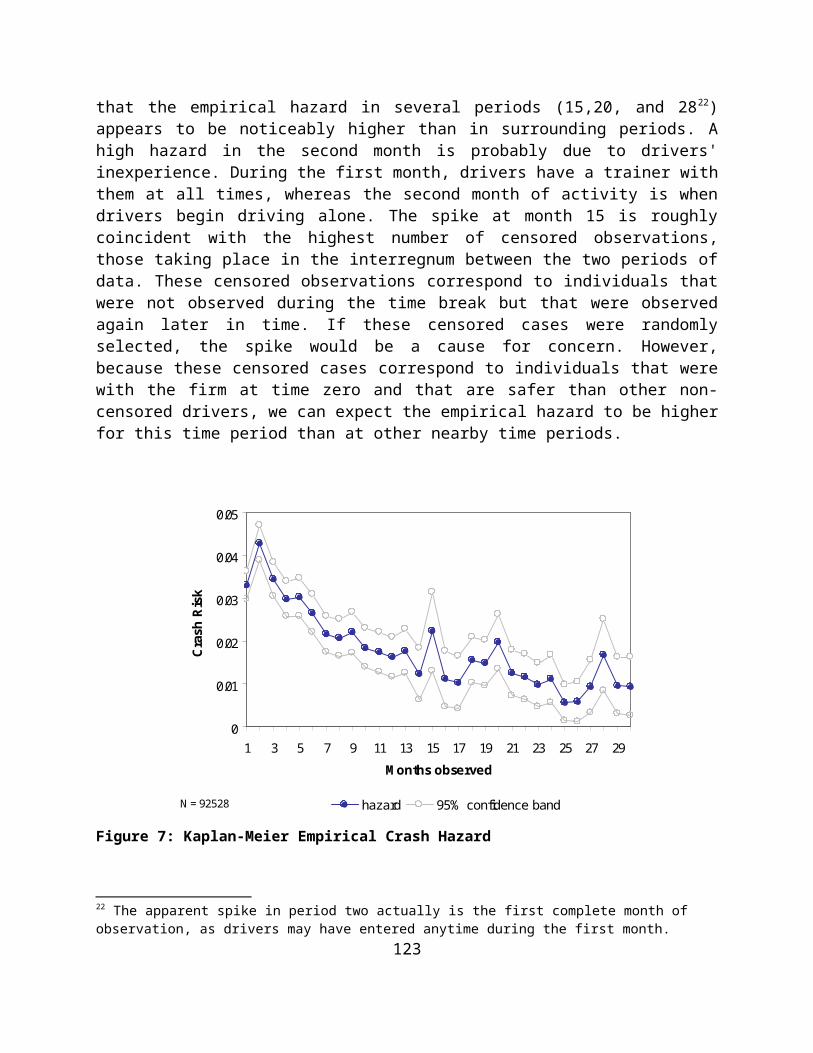
How much?

What method or methods do you use to pay your drivers for hooking? If there is more than one method, you can choose more than one.

No pay (Button should put zero amounts in b, c and d below)

Same as for dropping. (Button should make c, d and e below equal to Question #19 b, c, d)

By the hour. How much?

Flat amount. How much?

Other way.

What other way?How much?

Next we’d like to ask about pay for various kinds of waiting time at origin or destination.

Do you pay your drivers while they wait for loading or unloading to begin?YesNo (Skip to Question #24)

What method or methods do you use to pay your drivers for this? If there is more than one method, you can choose more than one.

By the hour. How much?

Flat amount. How much?

Other way.

What other way?How much?

Are there any requirements that must be met before receiving this pay such as a minimum amount of waiting time?

Yes. Please describe:

No

What percentage of your pickups involve only dropping or hooking at the point of origin?

What percentage of your deliveries involve only dropping or hooking at the point of destination?

What percentage of your runs involve the loading of freight by your drivers at the point of origin?

What percentage of your runs involve the unloading of freight by your drivers at the point of destination?

Section Two: Intermediate Stops

In this section we are going to ask questions about pay at intermediate stops. By an intermediate stop we mean a stop between the point of origin of a run and the point of destination of a run. We’ll ask about four different kinds of pay. The first is a flat amount of pay for making an intermediate stop; this is sometimes called stop pay. The second is pay for loading or loading done by the driver at an intermediate stop. The third is pay for monitoring loading or unloading, and the fourth is pay for waiting time.

First we’d like to ask about whether you pay drivers for making an intermediate stop.

Do you pay drivers a flat rate for making an intermediate stop?

Yes

No (Skip to Question #32)

How much is this flat rate?

Are there any requirements that must be met before receiving this pay such as a minimum amount of time spent at an intermediate stop?

Yes. Please describe:

No

Do you pay your drivers the same way for subsequent intermediate stops as they are paid for the first intermediate stop? If no, can you please explain how you pay them for subsequent intermediate stops?

Yes, the same way as for the first stopNo (please explain):

Next, we’d like to ask about pay when drivers load or unload the truck themselves at intermediate stops.

Do you pay drivers when they are required to load or unload freight at intermediate stops?

Yes No (Skip to Question #36)

How do you pay your drivers for this?

By the hour. How much? Flat amount per load. How much?Cents per hundredweight. How much? Cents per case. How much?Other method. What method and how much?

Are there any requirements that must be met before receiving this pay such as a minimum amount of freight which must be handled?

Yes. Please describe:

No

Is this pay for loading or unloading in addition to any flat rate that is paid for making an intermediate stop, or instead of this flat rate? Would you say this pay is A. ‘in addition to any flat rate’ or B. ‘instead of this flat rate?

In addition to any flat rate

Instead of this flat rate

What percentage of intermediate stops require the driver to load or unload freight?

Do you pay drivers at intermediate stops when they don’t do any loading or unloading themselves but are required to monitor or check the process of loading or unloading?

Yes

No (Skip to Question #40)

How do you pay your drivers for this?

By the hour. How much?Flat amount per load. How much?Cents per hundredweight. How much?Cents per case. How much?Other method. What method and how much?

Are there any requirements that must be met before receiving this pay such as a minimum amount of freight involved?

Yes. Please describe:

No

Next we’d like to ask about pay for waiting time at intermediate stops.

Do you pay your drivers while they wait for loading or unloading to begin?

YesNo (skip to Question #43)

What method or methods do you use to pay your drivers for this? If there is more than one method, you can choose more than one.

By the hour. How much?

Flat amount. How much?

Other way.

What other way?How much?

Are there any requirements that must be met before receiving this pay such as a minimum amount of waiting time?

Yes. Please describe:

No

What percentage of runs involve at least one intermediate stop?

(If answer to Question #43 is 0%, skip to question #47).

For those runs which have at least one intermediate stop, how many intermediate stops are there, on average?

How much elapsed time does a driver spend at the average intermediate stop?

Of this time, how much time is spent by the driver loading or unloading freight or monitoring the loading or unloading when it is done by someone other than the driver?

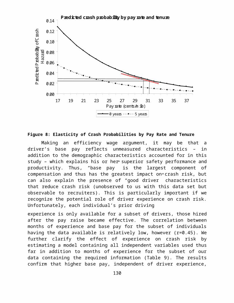
Section Three: Additional Questions

Is there some way drivers are paid at either origin or destination or at intermediate stops that we haven’t asked you about? If so, could you please describe what that is?

What proportion of your runs involve a destination which is a food distributor’s warehouse, a grocery warehouse or a store that sells groceries?

How many company solo drivers do you employ, not including owner-operators?

Solo drivers:

How many company teams do you employ, not including owner-operators?

Teams:

How many solo drivers do you run who are owner-operators or working for owner-operators?

Solo drivers:

How many teams do you run who are owner-operators or working for owner-operators?

Teams:

How many total miles did your firm operate in 1999?