Finance and Economics Discussion SeriesDivisions of Research & Statistics and Monetary Affairs

Federal Reserve Board, Washington, D.C.

Payday Loans and Consumer Financial Health

Neil Bhutta

2013-81

NOTE: Staff working papers in the Finance and Economics Discussion Series (FEDS) are preliminarymaterials circulated to stimulate discussion and critical comment. The analysis and conclusions set forthare those of the authors and do not indicate concurrence by other members of the research staff or theBoard of Governors. References in publications to the Finance and Economics Discussion Series (other thanacknowledgement) should be cleared with the author(s) to protect the tentative character of these papers.

Payday Loans and Consumer Financial Health Neil Bhuttaa

September 2013

Abstract: The annualized interest rate for a payday loan often exceeds 10 times that of a typical credit card, yet this market grew immensely in the 1990s and 2000s, elevating concerns about the risk payday loans pose to consumers and whether payday lenders target minority neighborhoods. This paper employs individual credit record data, and Census data on payday lender store locations, to assess these concerns. Taking advantage of several state law changes since 2006 and, following previous work, within-state-year differences in access arising from proximity to states that allow payday loans, I find little to no effect of payday loans on credit scores, new delinquencies, or the likelihood of overdrawing credit lines. The analysis also indicates that neighborhood racial composition has little influence on payday lender store locations conditional on income, wealth and demographic characteristics. JEL Codes: D14, G2 Key words: payday lending, credit scores, consumer financial protection, consumer finance, predatory lending, behavioral economics

a Board of Governors of the Federal Reserve Board. 20th and C St NW, Washington, DC, 20551. Email:

neil.bhutta@frb.gov. The views and conclusions expressed in this paper are those of the author and do not necessarily represent those of the Federal Reserve Board or System. Robert Sterling Letson, Shira E. Stolarsky and Peter Jacobson provided research assistance. Thanks to Kartik Athreya, Brian Bucks, David E. Buchholz, Glenn Canner, John Caskey, Jane Dokko, Gregory Elliehausen, Jacob Goldin, Tal Gross, Benjamin Keys, Michael D. Makowsky, Hilary B. Millar, Donald Morgan, Maureen C. Yap and an anonymous referee for very helpful comments.

1. Introduction

For a two-week $300 payday advance loan, payday lenders typically charge in excess of

$45, a cost so high that many believe the loan could not possibly be in the best interest of the

borrower. Nevertheless, some estimates indicate that payday loan volume grew more than five-

fold to almost $50 billion from the late 1990s to the mid 2000s (Stegman 2007). With the recent

rise of the payday lending industry, questions abound about the characteristics and circumstances

of payday loan borrowers, and the ultimate impact of such loans on their welfare. Interest in

payday lending has grown among economists in particular because of the possibility that

transactions in this market may reflect a market failure due to asymmetric information or

borrowers’ cognitive biases or limitations, or demonstrate divergence in behavior from

traditional models (hyperbolic discounting, for example).

In 2007, Congress and the Department of Defense moved to ban payday lending to

members of the military based on the view that such lending traps service members in a cycle of

debt and threatens military readiness.2 And in 2010, the Dodd-Frank Wall Street Reform and

Consumer Protection Act established the Consumer Financial Protection Bureau (CFPB) to help

regulate the market for consumer financial products, including the payday loan market.

Historically, regulation of payday lending to the general population has often come at the state

level, but the CFPB has authority to write and enforce new federal regulations to the extent that

they judge payday loans to be “unfair, deceptive or abusive,” and they have recently suggested

that new consumer protections in the payday loan market may be forthcoming (CFPB 2013).

In this paper, I draw on nationally representative panel data comprised of individual

credit records, as well as Census data on the location of payday loan shops at the ZIP code level,

to test whether payday loans affect consumers’ financial health. I use credit scores and score

changes, as well as other credit record variables, as measures of financial health. Credit scores

conveniently summarize one’s credit history, and previous research suggests payday loan usage

could affect credit scores. Importantly, use of and performance on payday loans does not

directly affect traditional credit scores (such as the FICO score). Rather, payday loans can affect

scores indirectly to the extent that such loans either improve or undermine consumers’ ability to

manage cash flow and meet their financial obligations in general.

2 See “Limitations on Terms of Consumer Credit Extended to Service Members and Dependents: Final Rule,” 72 Federal Register No. 169 (August 31, 2007), pp. 50580-50594 (http://www.gpo.gov/fdsys/pkg/FR-2007-08-31/pdf/07-4264.pdf).

1

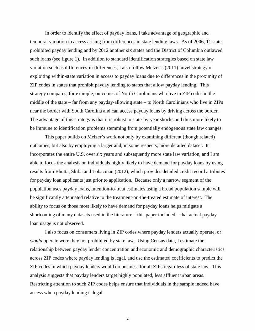
In order to identify the effect of payday loans, I take advantage of geographic and

temporal variation in access arising from differences in state lending laws. As of 2006, 11 states

prohibited payday lending and by 2012 another six states and the District of Columbia outlawed

such loans (see figure 1). In addition to standard identification strategies based on state law

variation such as differences-in-differences, I also follow Melzer’s (2011) novel strategy of

exploiting within-state variation in access to payday loans due to differences in the proximity of

ZIP codes in states that prohibit payday lending to states that allow payday lending. This

strategy compares, for example, outcomes of North Carolinians who live in ZIP codes in the

middle of the state – far from any payday-allowing state – to North Carolinians who live in ZIPs

near the border with South Carolina and can access payday loans by driving across the border.

The advantage of this strategy is that it is robust to state-by-year shocks and thus more likely to

be immune to identification problems stemming from potentially endogenous state law changes.

This paper builds on Melzer’s work not only by examining different (though related)

outcomes, but also by employing a larger and, in some respects, more detailed dataset. It

incorporates the entire U.S. over six years and subsequently more state law variation, and I am

able to focus the analysis on individuals highly likely to have demand for payday loans by using

results from Bhutta, Skiba and Tobacman (2012), which provides detailed credit record attributes

for payday loan applicants just prior to application. Because only a narrow segment of the

population uses payday loans, intention-to-treat estimates using a broad population sample will

be significantly attenuated relative to the treatment-on-the-treated estimate of interest. The

ability to focus on those most likely to have demand for payday loans helps mitigate a

shortcoming of many datasets used in the literature – this paper included – that actual payday

loan usage is not observed.

I also focus on consumers living in ZIP codes where payday lenders actually operate, or

would operate were they not prohibited by state law. Using Census data, I estimate the

relationship between payday lender concentration and economic and demographic characteristics

across ZIP codes where payday lending is legal, and use the estimated coefficients to predict the

ZIP codes in which payday lenders would do business for all ZIPs regardless of state law. This

analysis suggests that payday lenders target highly populated, less affluent urban areas.

Restricting attention to such ZIP codes helps ensure that individuals in the sample indeed have

access when payday lending is legal.

2

Interestingly, the analysis of payday lender locations does not indicate that lenders target

minority neighborhoods, conditional on economic characteristics of the population. This result is

important in its own right because of fair lending concerns that payday lenders target minority

neighborhoods without economic justification. Previous research on the determinants of payday

lender location has generally been limited to analyses of one city or nationally at a more

aggregated level such as the county (e.g. Prager 2009). Surprisingly, this is the first paper to use

readily available Census ZIP code business data to analyze the socioeconomic factors correlated

with payday lender concentration.

Finally, I also test whether access to payday loans interacts with shocks to the local

economy. The period studied covers the Great Recession and thus large unemployment shocks

at the county level are not uncommon in the data. This test has much in common with Morse

(2011), who finds that access to payday loans substantially mitigates foreclosures after natural

disasters.3

Overall, I find little to no effect of payday loans on consumers’ financial health, which

contrasts somewhat with recent research that finds both substantive positive and negative effects

of access to payday loans on financial well-being. For example, Morse (2011) finds that access

to payday loans lowers the likelihood of foreclosure after natural disasters by over 20 percent,

and Morgan and Strain (2008) find that loss of access to payday loans results in increased

bankruptcy filings. On the contrary, Skiba and Tobacman (2011) find that access doubles

chapter 13 bankruptcy filings, and Melzer (2011) finds that access increases the incidence of

having difficulty paying bills by 25 percent among lower-income households.

Thus, previous research suggests payday loans could affect credit scores, but the evidence

is mixed.4 The primary outcome variable studied in this paper – credit score – has the advantage

of summarizing consumers’ recent credit history and allowing detection of outcomes less severe

than events such as bankruptcy and foreclosure, and helps extend the range of outcomes studied

in the literature.5

3 Carrell and Zinman (2013) find that payday loans have a more negative effect on military personnel performance in areas with higher unemployment, although this is

4 As I discuss in Section 6, there are some plausible reasons for the differences in findings between various studies. See Caskey (2010) for an in-depth review of these papers.

5 Some other outcomes studied not mentioned elsewhere in the text include the incidence of bounced checks (Morgan, Strain and Seblani 2012), job performance (Carrell and Zinman 2013), and employment (Zinman 2010). Bhutta, Skiba and Tobacman (2012) also study credit scores and similarly find that payday loans have no

3

The available data do not allow for a full welfare assessment of access to payday loans,

but this analysis nevertheless helps inform the debate by testing for some of the potential costs

and benefits of access to payday loans. The next section also discusses the payday borrowing

process, the credit profile of people applying for payday loans, and state payday lending laws.

Section 3 presents the empirical strategy for estimating how payday loans affect financial health.

Section 4 focuses on the location of payday lenders and how state laws and neighborhood

socioeconomic factors have influenced payday lender locations. Section 5 presents estimates of

how payday loans affect financial well-being and Section 6 discusses these results further in the

context of past research. Finally, Section 7 concludes.

2. Background

2.1. Payday Loans and Financial Health

A payday loan is a 1-4 week loan of less than $1,000 that costs about $15-$30 per $100

borrowed, an annualized percentage rate of 360%-780% for a two-week loan. Payday loans are

usually provided by specialized finance companies that may also provide check cashing services,

rather than more mainstream financial institutions such as federally-insured banks. To qualify

for a payday loan, an applicant typically must show proof of residence, identification,

employment and a valid checking account, and must have some minimum level of monthly

earnings. If approved, applicants then provide the lender with a postdated check for the amount

of the loan and fee (or provide authorization to debit their checking account). Finally, the

application process does not involve a traditional credit check, and payday borrowing activity is

not reported to the national credit bureaus Equifax, Experian and TransUnion. This means that

payday borrowing is not a factor, like credit card borrowing, that directly affects one’s credit

score.6 Instead, access to payday loans can only affect one’s credit score indirectly depending on

how such loans affect consumers’ ability to meet their financial obligations in general.

On the one hand, usury laws that prohibit payday lending may inefficiently constrain

credit access, and lifting such bans would expand financial choices and allow individuals and

households to better manage their cash flow in the face of volatile income and expenses.

Although the fees can add up to large amounts, especially when loans are renewed multiple

effect, but in contrast to this paper, they use a regression discontinuity research design comparing those just above and below the payday loan approval threshold.

6 For an in-depth discussion of credit score modeling, see Board of Governors (2007).

4

times, these loans are often promoted by the payday loan industry as being meant for liquidity-

constrained individuals with a short-term emergency need for cash; for example, to help pay for

a necessary car repair or for out-of-pocket medical costs. In the absence of such credit, these

short term emergencies could become more costly than the ultimate cost of the loan if, for

instance, they lead to job loss or more severe medical problems.

On the other hand, potential payday loan customers may have behavioral biases or

limitations in analytical ability that make a ban on payday lending welfare enhancing. For

example, over-optimism about their ability to pay off the loan in 1-4 weeks may entice people to

use payday loans, when in fact they are likely to renew the loan several times (which lenders are

aware of), putting their financial well-being at risk. Indeed, administrative data on payday

borrowers collected by Skiba and Tobacman (2008) indicate that many payday borrowers renew

their loans several times, although it is not clear whether they expected, ex-ante, to renew so

many times or not. Even if borrowers expect to renew the loan several times, Bertrand and

Morse (2011) provide survey evidence that payday borrowers tend to get the math wrong. That

is, survey respondents typically did not correctly add-up (and, more importantly, underestimated)

the fees stemming from multiple renewals. Finally, by expanding credit at the margin, payday

loans could exacerbate perpetual liquidity problems and chronic dissaving due to time-

inconsistent preferences of hyperbolic discounters and again negatively affect lifetime utility.7

In this paper, I test whether access to payday loans affects credit scores. Credit scores are

heavily influenced by consumers’ payment history on their loans and lines of credit, and thus

reflect their ability to manage their financial obligations. Scores could be positively related to

access if payday loans provide an additional source of liquidity that can help people better

manage temporary cash flow shocks and keep them from missing payments on important

financial obligations.8 Some previous research provides evidence that payday loans help

mitigate the likelihood of major negative events such as foreclosure (Morse 2011) and

bankruptcy (Morgan and Strain 2008); studying credit scores has the advantage of being able to

detect more modest effects as well.

7 See Laibson (1997) for more on hyperbolic discounting and the welfare effects of expanded credit access. Skiba and Tobacman (2008) examine payday borrowing behavior using data from a payday lender and conclude that borrowing and repayment patterns are most consistent with partially naïve quasi-hyperbolic discounting.

8 That said, such a result does not necessarily imply that the benefits outweighed the cost of the loan.

5

Alternatively, previous research has also provided some evidence that payday loans may

be financially destabilizing and therefore could negatively affect credit scores. A substantive

negative relationship might reflect a market failure, perhaps related to the behavioral issues just

discussed, suggesting the need for regulation. The primary goal in this paper is to build on

previous research by quantifying the causal relationship between payday loans and credit scores.

If a large negative effect were to be found, it would lend support to the concerns about payday

loans.

2.2. The Credit Profile of Payday Loan Borrowers

A critical assumption in this paper is that payday loan borrowers actually have credit

records and credit scores that could be influenced (indirectly) by payday loan use. Existing

evidence shows that payday loan borrowers do indeed operate in the mainstream financial

system, which is perhaps not too surprising given payday loan borrowers must be employed and

have a checking account to qualify for the loan. For example, Elliehausen and Lawrence (2001)

present survey evidence that payday borrowers also apply for and use traditional forms of credit

(credit cards, car loans, etc.).

More recently, Bhutta, Skiba and Tobacman (2012; hereafter BST) provide

administrative evidence on the credit histories of payday loan applicants, matching applicant data

from a large payday lender to applicants’ credit records from Equifax. The data allow for a

precise match, and the matching results imply that essentially all payday loan borrowers have

credit records, and well over 90 percent have a credit score. Additionally, about 87 percent have

at least 1 open account at the time of applying for a payday loan, and the median debt balance

across all applicants (including those without any accounts) is about $6,000, compared to about

$9,000 for the general population. BST also find that about 60 percent of payday loan applicants

have at least one credit card account (compared to 75 percent of the general population), but the

cumulative credit limit across all card accounts is just $3,000 on average, compared to nearly

$19,000 for the general population.9

Two other characteristics of payday loan applicants that stand out are that they are

relatively young, and appear to be searching intensively for more traditional forms of credit.

BST document that payday applicants had, on average, over 5 credit inquiries (a proxy for credit

9 Note that the time period of the matched data in BST is the early 2000’s.

6

applications at traditional lenders that report to Equifax) in the 12 months leading up to their

application for a payday loan, compared to just one inquiry for the general population in the

same 12 month period, and 3 inquiries for the general subprime population.

As noted earlier, I draw on this information from BST to form a restricted sample of

consumers where the probability of using a payday loan, given access, is likely to be much

higher than for the population at large. Restricting the sample will help provide a better sense of

the potential size of the true effect of payday loans on financial well-being.

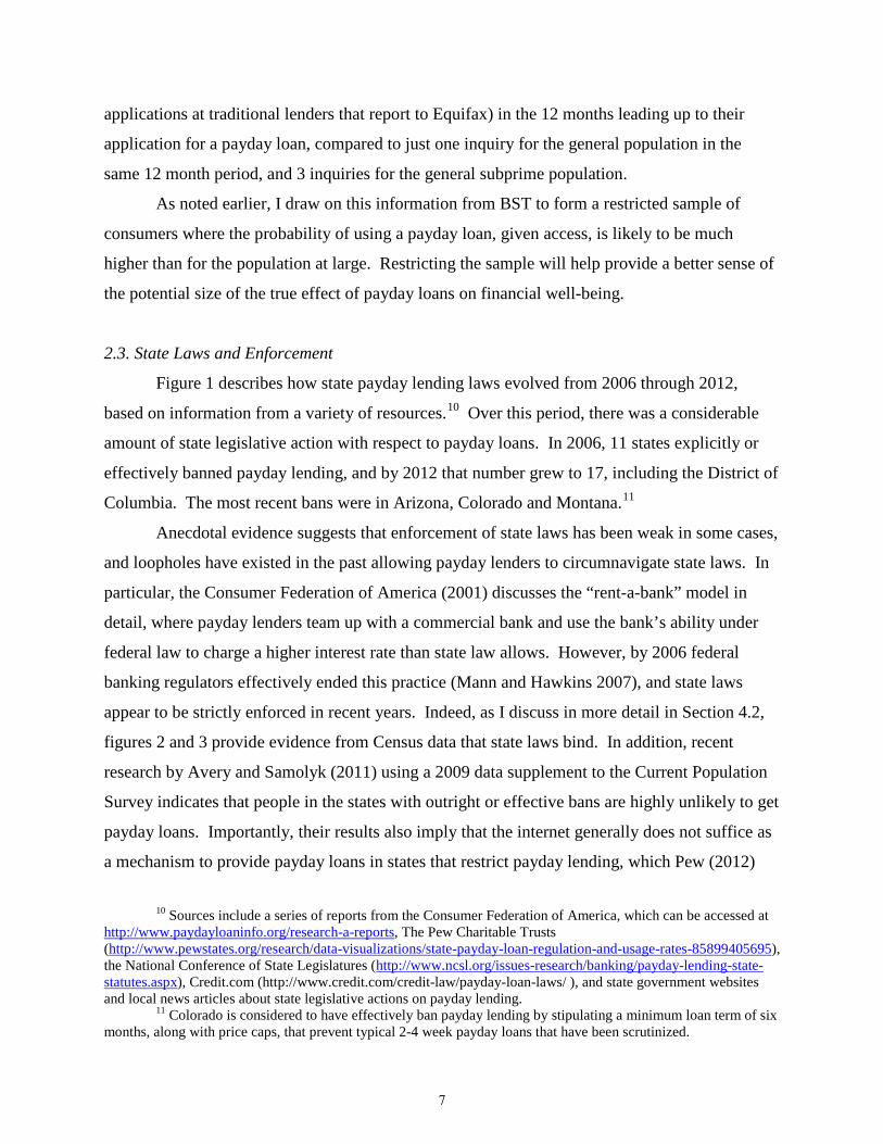
2.3. State Laws and Enforcement

Figure 1 describes how state payday lending laws evolved from 2006 through 2012,

based on information from a variety of resources.10 Over this period, there was a considerable

amount of state legislative action with respect to payday loans. In 2006, 11 states explicitly or

effectively banned payday lending, and by 2012 that number grew to 17, including the District of

Columbia. The most recent bans were in Arizona, Colorado and Montana.11

Anecdotal evidence suggests that enforcement of state laws has been weak in some cases,

and loopholes have existed in the past allowing payday lenders to circumnavigate state laws. In

particular, the Consumer Federation of America (2001) discusses the “rent-a-bank” model in

detail, where payday lenders team up with a commercial bank and use the bank’s ability under

federal law to charge a higher interest rate than state law allows. However, by 2006 federal

banking regulators effectively ended this practice (Mann and Hawkins 2007), and state laws

appear to be strictly enforced in recent years. Indeed, as I discuss in more detail in Section 4.2,

figures 2 and 3 provide evidence from Census data that state laws bind. In addition, recent

research by Avery and Samolyk (2011) using a 2009 data supplement to the Current Population

Survey indicates that people in the states with outright or effective bans are highly unlikely to get

payday loans. Importantly, their results also imply that the internet generally does not suffice as

a mechanism to provide payday loans in states that restrict payday lending, which Pew (2012)

10 Sources include a series of reports from the Consumer Federation of America, which can be accessed at http://www.paydayloaninfo.org/research-a-reports, The Pew Charitable Trusts (http://www.pewstates.org/research/data-visualizations/state-payday-loan-regulation-and-usage-rates-85899405695), the National Conference of State Legislatures (http://www.ncsl.org/issues-research/banking/payday-lending-state-statutes.aspx), Credit.com (http://www.credit.com/credit-law/payday-loan-laws/ ), and state government websites and local news articles about state legislative actions on payday lending.

11 Colorado is considered to have effectively ban payday lending by stipulating a minimum loan term of six months, along with price caps, that prevent typical 2-4 week payday loans that have been scrutinized.

7

concludes as well in separate research. Consistent with those findings, the websites of the largest

payday lending companies appear to prohibit applications from people residing in states that

restrict such loans.

3. Empirical Strategy

3.1. Main Specifications

The primary goal of this paper is to estimate the effect of payday loans on financial well-

being. To that end, I exploit within-state variation in access to payday loans arising from

changes in state laws, as well as across-ZIP-code variation within payday-prohibiting states, as in

Melzer (2011), in the following regression specification:

1 2

3 4 5

( ) ( )( ) ( ) ( )

izcst zt zt ct

ct zt ct i s t izcst

y PDaccess PDaccess unemp shockunemp shock border HPIgrowth

α β ββ β β γ µ ε

= + + ⋅′+ + + + + + +x δ

(1)

The dependent variable is a measure of financial well-being from the credit record data

(discussed later) for individual i, in ZIP code z, county c, state s and year t. As discussed earlier,

payday loan access (PDaccess) varies at the ZIP code level because in states where payday

lending is banned, some ZIP codes in those states will still have access because of their close

proximity to states that allow payday lending. Following Melzer (2011), I consider a ZIP code in

a ban state to have access if it is less than 25 miles from a ZIP code in another state that allows

payday lending.

I also interact payday loan access with county unemployment shocks, measured as the

difference between the unemployment rate in year t and the average unemployment rate for the

county from 2000 to 2006. Although someone who loses his job may not be able to get a payday

loan because they no longer have a regular paycheck (although a regular unemployment check

may suffice), a spouse or other member of the household may still be able to access payday

loans. A household suffering from an income shock may turn to payday loans to help smooth

consumption, expecting that the lost income will soon be replaced from a new job. However,

borrowers may systematically overestimate the likelihood of replacing their income, and payday

loans could then make a tough financial situation even worse. Alternatively, borrowers could

use the proceeds of a payday loan to help make minimum payments on other financial

8

obligations to avoid becoming delinquent on accounts that get reported to credit bureaus and feed

into their credit score.

The specification also includes controls for whether a ZIP code borders another state;

house price appreciation at the county level over the previous two years in order to help control

for the extent of the housing bust; and a vector x of socioeconomic characteristics.12 Finally,

equation (1) includes state fixed effects and time fixed effects and thus, as noted earlier, the

effect of access to payday loans will be identified from within-state variation.

There are three sources of within-state variation. First, residents of a given state can lose

access to payday loans simply because their state implements a ban of such loans. Second, some

residents of states with a ban still have access through a bordering state if they live close to the

border, whereas other residents of the same state living in the interior do not have access. And

third, those who have access through a border state can lose access when that bordering state

implements a ban. For example, residents of Massachusetts who had access to payday loans

through New Hampshire lost that access in 2009 when New Hampshire imposed a ban.

A benefit of the detailed data used in this paper is that state-by-year fixed effects, which

control for state-year shocks that could be correlated with state law changes and outcomes, can

be included:

1 2

3 4 5

( ) ( )( ) ( ) ( )

izcst zt zt ct

ct zt ct i st izcst

y PDaccess PDaccess unemp shockunemp shock border HPIgrowth

α β ββ β β η ε

= + + ⋅′+ + + + + +x δ

(2)

Identification in this specification comes from the second and third sources of variation just

discussed. Obviously, a key assumption is that people actually cross state borders to get payday

loans. Anecdotal evidence suggests this occurs, and Melzer (2011) provides evidence that

payday lenders open shops along borders with payday-prohibiting states, presumably because

people will travel across the border to get payday loans. In Section 4.4, I provide similar

evidence.

3.2. Regressions Using a Restricted Sample

12 Although x has a subscript i, I am mostly limited to using census tract proxies for individual characteristics. Census tracts are considerably smaller geographic areas than ZIP codes and are designed to be relatively homogenous with respect to socio-economic characteristics.

9

As a starting point, equations (1) and (2) are estimated using an unrestricted sample

representing all consumers in the U.S.. However, because only a narrow segment of the

population typically uses payday loans, estimates of β1 and β2 will be substantially smaller than

the treatment-on-the-treated estimates of the effect of payday loan borrowing that are ultimately

of interest.13 In other words, because borrowing on payday loans is not directly observed in the

data, and because the probability of payday loan use is small, the reduced form estimates from

equations (1) and (2) will be attenuated relative to the estimates of interest.

To address this issue, I also estimate equations (1) and (2) using a restricted sample of

consumers where the probability of borrowing on payday loans given access is likely to be much

higher. I restrict the sample along two dimensions. The first dimension relates to individual

characteristics that have been shown in past research to be closely related to payday loan use, as

discussed will be discussed in more detail in Section 5.1. The second dimension relates to where

individuals live, and whether their residential ZIP code location is the type of area that actually

attracts payday lenders – for example ZIP codes with a high enough concentration of people with

potential demand for payday loans in order to operate profitably.14

3.3. Identifying “Payday ZIPs”

In order to identify ZIP codes that are attractive to payday lenders, I run a negative

binomial regression of the count of payday stores in a given ZIP code, z, in 2008 on two scale

variables (ZIP code population and ZIP code total number of establishments) and a variety of

ZIP code socioeconomic characteristics:15

{ }0 1 2( ) exp ln( ) ln( )z z z zE PDstores pop estabα α α ′= + + + x β (3)

Equation (3) is estimated using only those ZIP codes in states that allowed payday lending

throughout the 2006-2012 period, and then I generate predictions of the number of payday loan

stores across ZIP codes in all states using the estimated coefficients (that is, both in-sample and

13 For example, Avery and Samolyk (2011) find that less than 5 percent of households report having used payday loans at least once during 2008.

14 This restriction may be less important for estimates of equation Error! Reference source not found. since they are identified from people who must travel to other to get payday loans anyway. On the other hand, payday lenders might only operate in places along the border if there are ZIP codes just across the border that would have attracted payday lenders had state law not prohibited them.

15 Negative binomial regression is a more general version of Poisson regression that allows the variance to exceed the mean.

10

out-of-sample predictions). Finally, I construct expected payday stores per capita (PDpercap)

for every ZIP code as:

zz

z

PDstoresPD percappopulation

= (4)

and define “payday ZIPs” as those ZIP codes with

zPD percap in the top one-third of ZIP codes.

4. Where Do Payday Lenders Operate? Evidence from Census Data

4.1. ZIP Code Socioeconomic and Payday Lender Location Data

I employ two primary sources of data to estimate equation (3) and obtain estimates of

neighborhood payday store concentration. The first are Census ZIP Code Business Patterns

(ZCBP) data, and the second are ZIP code socioeconomic characteristics from the 2000 Census.

The ZCBP data have been published annually since 1994, and measure the number of

establishments, number of employees and total payroll by ZIP and detailed industry code.16 Two

North American Industrial Classification System (NAICS) codes in particular capture payday

lending establishments:

1) Nondepository consumer lending (522291): establishments primarily engaged in making

unsecured cash loans to consumers

2) Other activities related to credit intermediation (522390): establishments primarily

engaged in facilitating credit intermediation (except mortgage and loan brokerage; and

financial transactions processing, reserve, and clearinghouse activities), including check

cashing services and money order issuance services

In 2008, there were about 14,500 establishments in industry 522291 and just over 20,000

establishments in industry 522390 across the entire U.S. The total number of payday

establishments based on the ZCBP may be on the high side (for instance, Stegman (2007) cites

industry figures estimating a total of around 25,000 storefronts) because not all check-cashing

outlets, especially those in states that prohibit payday lending, necessarily offer payday loans.

Also, these six-digit NAICS industries can include other types of businesses besides payday

lenders and check-cashers to the extent that they still fit within the industry definition.

16 Note that these data exclude information on non-employer firms. For more information on the ZCBP data, see http://www.census.gov/econ/cbp/index.html.

11

Although the ZCBP data provide a noisy measure of payday lending stores in a given ZIP

code, my interest lies in the geographic variation of stores rather than in their total number, and

therefore the ZCBP should serve the analysis well. Indeed, state-level variation in the number of

establishments per person follows expected patterns. For instance, several southern states

(Mississippi, South Carolina and Louisiana) have the highest number of payday establishments

per person, which is very similar to Prager’s (2009) finding.

Table 1 provides summary statistics from the ZCBP and the 2000 Census data. The

sample of ZIP codes includes only those in states that allowed payday lending throughout the

2006 to 2012 period (excluding Alaska and Hawaii); those in metropolitan areas; and those with

at least one establishment employee, at least 1000 residents, and no more than 50 percent of the

population residing in group quarters. These restrictions yield a sample of 8,666 ZIP codes, with

an average population of just over 17,000.

On average, these ZIP codes contain about 400 establishments across all industries, and

about 2.4 establishments in the payday lending industries. The median ZIP code, however,

contains just one payday industry establishment. The other variables listed help describe the

income, wealth and demographic characteristics of the ZIP codes, which may influence the

demand for payday loans. Median family income ranges from about $32,000 at the 10th

percentile to over $75,000 at the 90th percentile. Median home value and the homeownership

rate also vary considerably across ZIP codes, as does educational attainment. Finally, as Caskey

(2005) notes, previous survey research indicates that payday loan customers tend to be young

and also tend to be female. I will therefore include the share of adults under the age of 40 and

the single-mother share of families as additional predictors of the number of payday lending

establishments.

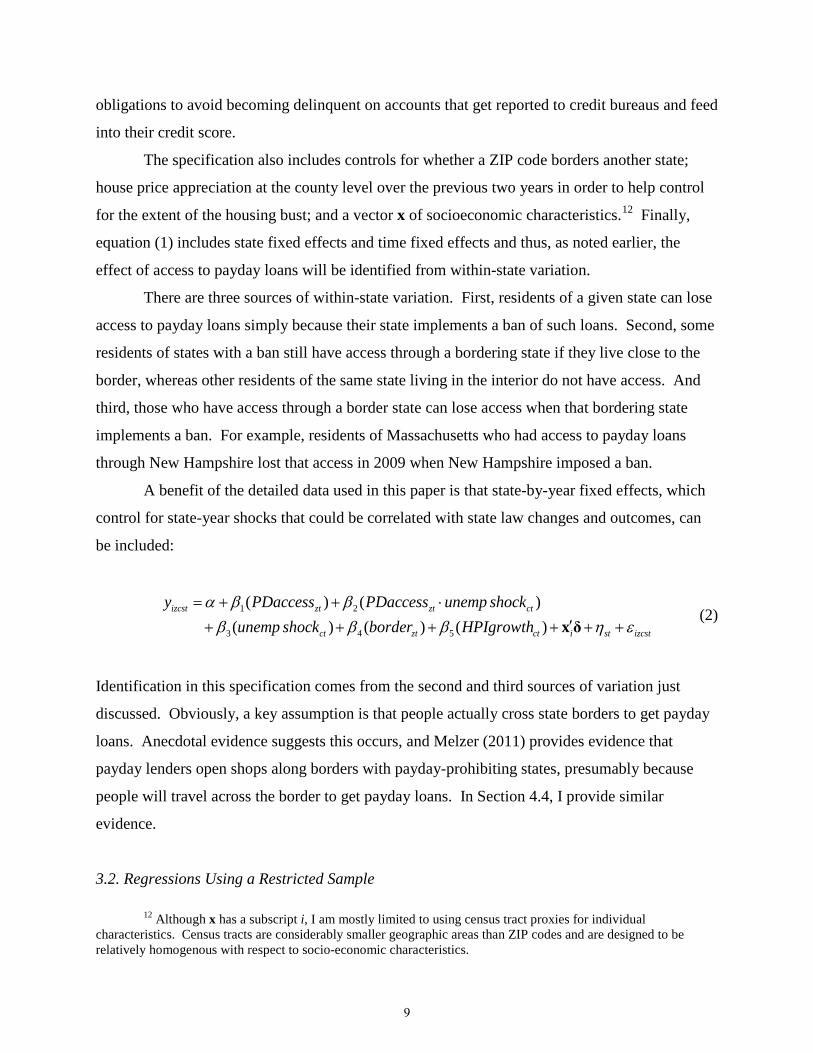
4.2. Are Payday Lending Laws Binding?

The ZCBP data suggest that state payday lending restrictions have had bite in recent

years. Figure 2 indicates that the state-level concentration of payday lending stores is

considerably higher in states that permit payday lending, whereas the concentration of

establishments in another nondepository consumer credit industry (522292 – real estate credit) is

much more similar across the two groups of states. (As noted above, because the industry codes

12

used to identify payday lenders include non-payday-lending establishments, the concentration of

establishments in these industries is not expected to be zero in payday-prohibiting states.)

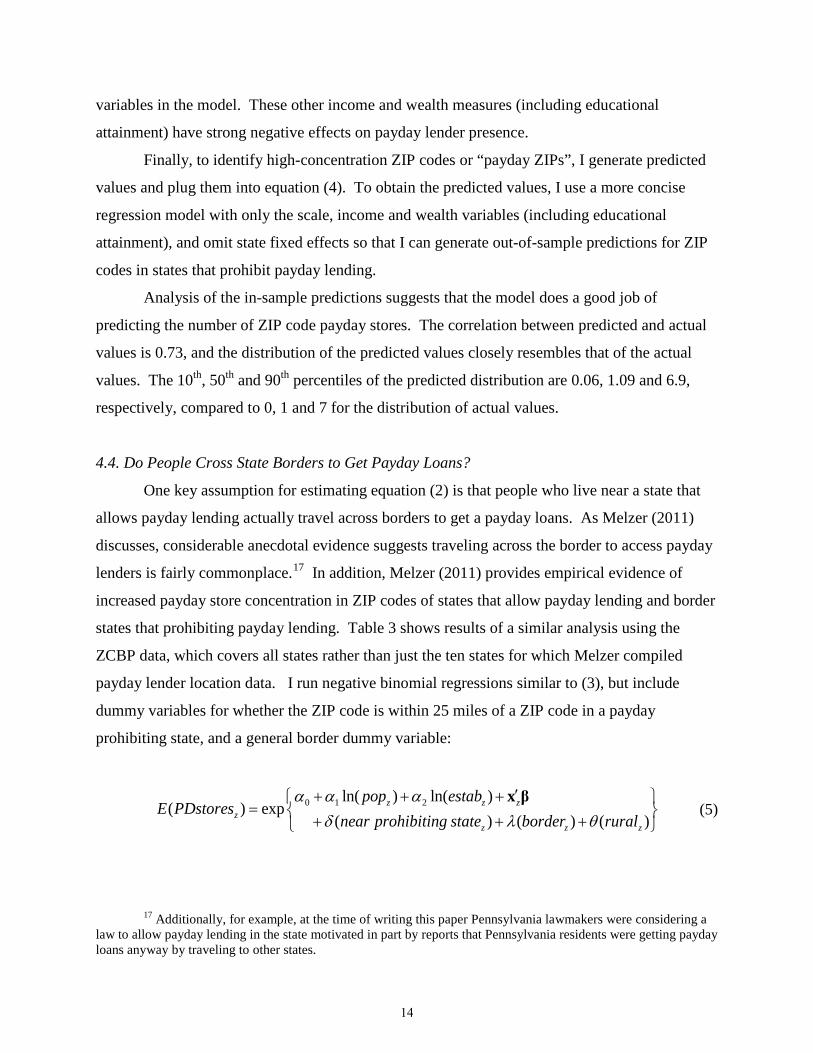
Figure 3 indicates that the concentration of payday lending stores declined by about 50

percent from 2006 through 2011 in the states that passed laws prohibiting payday lending during

this period (black bars). In 2007, the concentration of payday lending stores in these states was

almost double the concentration in states where payday lending was prohibited throughout the

period. But by 2011, the concentrations in these two groups of states were nearly identical. To

be sure, there was a slight down trend in concentration in states that allowed payday lending

throughout the period, but this trend was not nearly as pronounced as for the states that

implemented bans or significant restrictions.

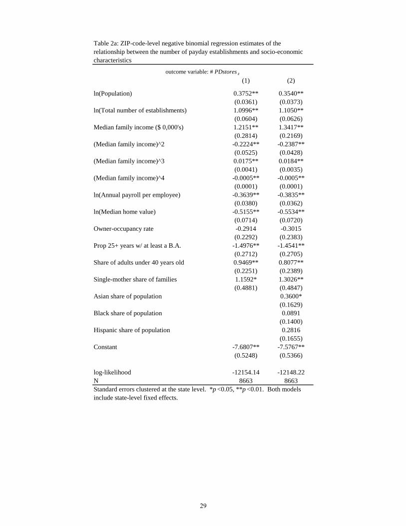
4.3. Socioeconomic Determinants of Neighborhood Payday Lender Concentration

Table 2a displays negative binomial (similar to Poisson regression) estimates of equation

(3). As noted in the introduction, these results are of interest in their own right because of

concerns about predatory lending and the concentration of payday lenders in minority

neighborhoods. With that in mind, I estimate two models, the first leaving out race and ethnic

composition variables and the second including them. Each specification allows for a nonlinear

relationship between the number of payday industry establishments and median family income,

and includes state fixed effects. Standard errors are clustered at the state level.

The second column of table 2a shows that one of the three race/ethnicity variables is

statistically significant, and the likelihood ratio test statistic rejects the hypothesis that all three

minority coefficients are zero. But as table 2b shows, the magnitudes of these coefficients are

quite small. For example, a one standard deviation increase in the Black population share (an

increase of 18 percentage points) would increase the number of payday stores by just 2 percent,

all else equal. In contrast, home values, educational attainment and median family income are

strongly related to the number of payday stores. Payroll per worker (the wages of local

employees, not necessarily residents of the ZIP code) also appears to have a strong relationship

with the number of payday lenders. Interestingly, a rise in median family income from $40,000

to $60,000 appears to have a positive effect on the number of payday establishments, but that

effect is of course conditional on local wages, home values, educational attainment and the other

13

variables in the model. These other income and wealth measures (including educational

attainment) have strong negative effects on payday lender presence.

Finally, to identify high-concentration ZIP codes or “payday ZIPs”, I generate predicted

values and plug them into equation (4). To obtain the predicted values, I use a more concise

regression model with only the scale, income and wealth variables (including educational

attainment), and omit state fixed effects so that I can generate out-of-sample predictions for ZIP

codes in states that prohibit payday lending.

Analysis of the in-sample predictions suggests that the model does a good job of

predicting the number of ZIP code payday stores. The correlation between predicted and actual

values is 0.73, and the distribution of the predicted values closely resembles that of the actual

values. The 10th, 50th and 90th percentiles of the predicted distribution are 0.06, 1.09 and 6.9,

respectively, compared to 0, 1 and 7 for the distribution of actual values.

4.4. Do People Cross State Borders to Get Payday Loans?

One key assumption for estimating equation (2) is that people who live near a state that

allows payday lending actually travel across borders to get a payday loans. As Melzer (2011)

discusses, considerable anecdotal evidence suggests traveling across the border to access payday

lenders is fairly commonplace.17 In addition, Melzer (2011) provides empirical evidence of

increased payday store concentration in ZIP codes of states that allow payday lending and border

states that prohibiting payday lending. Table 3 shows results of a similar analysis using the

ZCBP data, which covers all states rather than just the ten states for which Melzer compiled

payday lender location data. I run negative binomial regressions similar to (3), but include

dummy variables for whether the ZIP code is within 25 miles of a ZIP code in a payday

prohibiting state, and a general border dummy variable:

0 1 2ln( ) ln( )( ) exp

( ) ( ) ( )z z z

zz z z

pop estabE PDstores

near prohibiting state border ruralα α α

δ λ θ′+ + +

= + + +

x β (5)

17 Additionally, for example, at the time of writing this paper Pennsylvania lawmakers were considering a law to allow payday lending in the state motivated in part by reports that Pennsylvania residents were getting payday loans anyway by traveling to other states.

14

I also include both rural and urban ZIP codes (of payday-allowing states) in the regression

sample since payday lenders might also increase their presence in rural ZIP codes on borders,

and I include a rural indicator variable in the regression.

The first column of table 3 shows a 12 percent increase in the number of payday stores in

ZIP codes within 25 miles of a ZIP code in a payday prohibiting state relative to other ZIP codes

in the same state, but the estimate is not quite statistically significant at the 5 percent level. The

second column regression employs a quadratic in distance to other states, rather than the border

dummy variable. The point estimate now is slightly larger (almost 15 percent) and statistically

significant. The final column presents an estimate using only ZIP codes that are near a state

border (that’s why the sample size drops significantly). This specification identifies δ more

stringently; the estimate indicates that ZIP codes near prohibiting states have 18 percent more

payday lending stores, on average, relative to other border ZIP codes in the same state that are

near other payday-allowing states. Notably, this estimate is quite similar in magnitude to

Melzer’s, and provides supportive evidence for the notion that people cross borders to obtain

payday loans.

5. Do Payday Loans Affect Financial Well-Being?

5.1. Consumer Credit Record Data and Outcome Measures

The credit record data used in this paper come from the Federal Reserve Bank of New

York Consumer Credit Panel/Equifax (CCP), a nationally representative longitudinal database

with detailed information at a quarterly frequency on consumer debt and loan performance

derived from consumer credit records maintained by Equifax, one of that nation’s three major

credit bureaus. 18 The CCP can be used to compute both nationally representative estimates at

the end of a given quarter as well as to track changes in debt use and loan performance for a

given individual over time.19

The CCP includes each person’s year of birth, and the ZIP and census tract codes of their

mailing address each quarter. With these geographic codes, I am able to merge the ZIP-level

predictions on payday lender concentration and census tract level socioeconomic characteristics

18 Lee and van der Klaaw (2010) provide a detailed discussion of these data. 19 All individuals in the database are anonymous: names, street addresses and social security numbers have

been suppressed. Individuals are distinguished and can be linked over time through a unique, anonymous consumer identification number assigned by Equifax.

15

from the 2000 Census to use as controls (in lieu of individual demographic data beyond age).

Finally, in addition to detailed credit account information, the CCP also provides a credit score

for most individuals, updated each quarter.20 The Equifax credit score, like other credit scores,

essentially summarizes the information in one’s credit report and is based on a model that

predicts the likelihood of becoming 90 days or more delinquent over the next 24 months. Credit

scoring models include numerous factors such as the frequency and degree of delinquent

accounts, the amount of credit being utilized, and recent applications for credit. Factors that are

not considered include income and employment history as such information is not available in

credit reports. The credit score ranges from 280-850, with a higher score corresponding to lower

relative risk.

I drew three independent cross-sections of the data for 2007, 2009 and 2012, and in each

cross section individuals are observed at both the beginning and end of the year.21 Table 4

provides summary statistics for the four outcomes examined in the regressions: credit score at the

end of the year, the probability of a score drop of 25 points or more over the course of the year,

the probability of a new delinquency, and the probability of hitting one’s credit limit on credit

cards (general purpose and retail cards) conditional on utilizing less than 75 percent at the start of

the year.22 Panel A shows statistics for the full sample of consumers. The average credit score is

almost 700, while the probability of experiencing a score decline of 25 percent or more is nearly

17 percent. The likelihood of a new delinquency is about 9 percent.23 Finally, the probability of

reaching or exceeding one’s credit card limit is just 2.4 percent.

Panel B restricts the sample to those living in “payday ZIPs” (see Section 4.3). This

restriction cuts the sample roughly in half, but the credit record statics are quite similar to the full

sample. In other words, people living in the urban areas where payday lenders most likely to be

highly concentrated are, on average, quite similar to the broad population in terms of their credit

20 Some individuals at a point in time are not “scoreable” because of a limited credit history. The Equifax credit score is similar to the well-known FICO risk score. For more details, see https://help.equifax.com/app/answers/detail/a_id/244/related/1.

21 I start with 2007 as opposed to 2006 because it comes after the FDIC guidance on the “rent-a-bank” model. Each cross section is an independent 25 percent of the full CCP.

22 FICO considers score changes of less than 20 points as indicative of stability. See for instance http://bankinganalyticsblog.fico.com/2010/07/how-much-do-fico-scores-change-over-time.html.

23 The CCP does not have account level information, but rather provides information on all accounts rolled up to the credit category level for ten different types of credit (e.g. credit cards, auto loans, etc.), such as the number of open accounts and the number of accounts in good standing. I identify individuals with a new delinquency as those who have at least one non-current account at the end of the year in a credit category in which they had at least one open account in that category at beginning of the year with all open accounts in the category in good standing.

16

record characteristics. Finally, Panel C restricts the sample further to borrowers likely to have

high demand for payday loans. Based on information from BST (2012), the sample includes

relatively young borrowers age 25-49, with no more than a $5,000 cumulative credit limit on

credit cards at the start of the year, and who inquired about credit at least twice in the prior

year.24 Notably, the sample size drops by almost 90 percent, which seems appropriate given

estimates that only about 5-10 percent of the population uses payday loans in a given year. This

group has considerably lower credit scores than the general population, and are more likely to

experience a score drop in excess of 25 points. The probability of a new delinquency is more

than double what it is for the general population, and the probability of maxing out their credit

card lines is substantially higher too. The regressions will test whether access to payday loans

improves or worsens these outcomes.

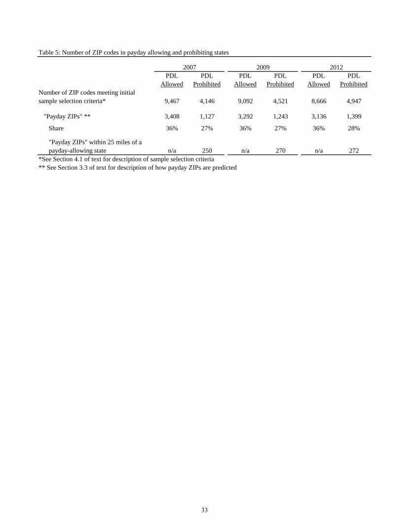
Table 5 shows the distribution of ZIP codes and payday ZIPs across payday allowing and

prohibiting states over time in 2007, 2009 and 2012. Between 2007 and 2009, about 800 ZIP

codes move from the allowed group to the prohibited group, an increase of about 20 percent. As

noted earlier, I define payday ZIPs as ZIP codes with a predicted payday lender concentration in

the top one-third of all ZIP codes. Thus, of the 13,613 ZIP codes initially in the sample, one-

third or 4,535 are payday ZIPs, and in 2007, 3,408 of these ZIPs were in payday allowing states

and 1,127 were in payday prohibiting states.25 By 2012, the number of payday ZIPs in

prohibiting states increased by about 24 percent to 1,399.

The last row of table 5 shows the number of payday ZIPs in prohibiting states within 25

miles of a payday allowing state. There were 250 such ZIP codes in 2007, rising to just 272 by

2012. The steadiness of this number masks the fact that some ZIP codes fall out of this group

over time (for example ZIP codes in Massachusetts near the border with New Hampshire lost

access in 2009 when New Hampshire implemented a ban), and others enter (for example border

ZIP codes in Arkansas that maintained access to payday loans through Tennessee despite the

state’s ban).

24 Credit inquiries refer to specific instances when a lender requests a credit report for an individual because that individual was seeking a new credit account. Inquiries do not include instances when lenders pull credit reports without an individual’s consent in order to conduct targeted marketing campaigns or for routine risk management procedures. Inquiries also do not include instances when a consumer requests his or her own credit report for monitoring purposes.

25 Since the District of Columbia (DC) allowed payday loans for most of 2007, DC is considered an allowing state for 2007.

17

5.2. The Effect of Payday Loans on Credit Scores

Table 6 presents estimates of the effect of payday loans on credit scores and the

probability of a score drop of at least 25 points. The first three columns show results for the

level of credit scores using an unrestricted sample of consumers. In addition to the specifications

discussed earlier with state fixed effects and state-by-year fixed effects, the first column shows

estimates only with region-by-year fixed effects, thus allowing cross-state variation to help

identify the effect of payday loans. The point estimate on the access variable in this regression

implies that access to payday loans leads to a reduction in credit scores of just -2.86 points (note

that the unemployment shock variable has been re-centered to have mean zero so that the

coefficient on the access to payday loans variable is roughly equivalent to what it would be in a

regression excluding the interaction term). The second column reports the results from

estimating equation (1), which one might find more persuasive as it includes state fixed effects,

but the result is little changed. The point estimate in this specification is only -1.14 points with a

standard error, clustered at the state level, of 1.37 points. Finally, the third column reports

results from estimating equation (2), which mirrors Melzer’s (2011) identification strategy by

including state-by-year fixed effects. Again, the point estimate is close to zero and insignificant.

The second row indicates that unemployment shocks have a statistically significant, but

small, negative effect on credit scores in places that prohibit payday loans. As noted earlier, the

unemployment shock variable is defined as the average unemployment rate in either 2007, 2009

or 2012 minus the average unemployment rate from 2000-2006; it has a standard deviation of

about 2.5 percentage points. The small effect of this variable probably stems from county-level

unemployment providing a rather noisy measure of individual unemployment. The coefficient

on the interaction with payday loan access is also close to zero and insignificant. Thus, overall

the regression results so far provide no evidence that payday loans affect credit scores.

As discussed in Section 3.2, one reason why the estimated effect over the unrestricted

sample might be so close to zero is that the probability of using payday loans among the broad

population is small. The next 3 columns show results for the same three specifications but using

only the restricted sample of individuals, described in the previous section, most likely to have

high demand for payday loans. The results over the narrow sample change sign (the effect of

payday loans is now positive), but the point estimates remain close to zero. The largest estimate

18

is in the middle column and is statistically significant, but the magnitude is only 2.8 points and

the 95 percent confidence interval rules out effects in excess of 5.3 points.

The second half of table 6 presents estimates of the effect of payday loans on the

probability of a score drop of 25 points or more over the course of the year. Focusing on the last

two columns where the restricted sample is used and state and state-year fixed effects are

included, respectively, the point estimates are negative (implying payday loans are beneficial)

but close to zero and insignificant.

The sign on the interaction term in the last two regressions indicates that payday loans are

more beneficial in places hit hard by labor market shocks, but the magnitude of the estimates are

fairly small, which again may reflect the weakness of the correlation between county level

unemployment and individual unemployment. With more precise data on individual

employment status, it seems possible that the interaction effect could be economically important,

but such data unfortunately are not available.26

5.3. Other Outcomes

Table 7 provides estimates the effect of payday loans on the likelihood of a new

delinquency, and the likelihood of reaching or exceeding one’s credit card limit. These two

variables are closely connected to variables that play an important role in determining one’s

credit score.

The first two columns of table 7 show the preferred specifications with state and state-

year fixed effects, respectively, over the restricted sample, and indicate a negative effect of

payday loans on the likelihood of delinquency (that is, payday loans tend to be helpful in

avoiding delinquency on traditional accounts), but the point estimates are small and statistically

insignificant. Labor market shocks appear to have a significant effect on the likelihood of

delinquency – a one standard deviation increase in the size of a county unemployment shock

leads to about a two percentage point increase in the likelihood of a new delinquency. The sign

on the interaction term is negative, suggesting that access to payday loans helps mitigate the

negative effect of a labor market shock, but the estimate is not statistically significant.

26 In contrast, Carrell and Zinman (2013) provide some evidence that high local unemployment exacerbates the negative effect of payday loans on military personnel performance. Although military personnel are, of course, employed, high unemployment could affect the employment status of a spouse and overall household income.

19

The last two columns of table 7 provide estimates of the effect of payday loans on the

likelihood of hitting one’s credit card limit. Again the point estimates are fairly small and

statistically indistinguishable from zero.

5.4. Alternative Samples and Specifications

Table 8 provides alternative estimates of the effect of payday loans based on additional

restrictions to the high payday loan demand subsample, as well as additional specifications

where initial credit score is included as a control. The first two columns show estimates of the

coefficient on the access variable in equations (1) and (2) using the restricted sample, but with

the additional restriction of excluding those with initial credit scores in excess of 600. Panel A

shows estimates for the effect of payday loans on credit scores at the end of the year. Though

both point estimates are statistically significant, they are slightly smaller than in table 6 (fifth and

sixth columns). As shown in the next two columns, after controlling for initial credit score, the

coefficient is more precisely estimated but even smaller in magnitude at less than 1.5 points.

The next four columns provide estimates where the high demand subsample has a

different additional restriction, limiting the sample to those with at least four inquiries in the past

year instead of two. The first two estimates are again statistically significant, but small, and are

not robust to controlling for initial credit score as seen in the last two columns.

Panels B, C and D provide estimates for the other three outcome variables. In general,

the estimates point in the direction of payday loans being beneficial, but the magnitudes are

small and insignificant. Perhaps a slight exception is that payday loans appear to reduce the

likelihood of a 25 point score drop by about 1 percentage point, on average, for the low initial

credit score subsample, but that is relative to a mean likelihood for this subsample of about 24

percent.

6. Discussion

Unlike previous research that finds both substantive positive and negative effects of

payday loans on financial well-being, the empirical results in this paper suggest little connection

(slightly beneficial, if anything). Differences in identification strategies could play some role in

generating different results. For example, Skiba and Tobacman (2011) use data from a payday

lender on a large set of applicants, exploit a discontinuity in the approval process, and find that

20

payday loans increase the likelihood of (chapter 13) bankruptcy. But, as they point out, the

estimated effect pertains to individuals near the discontinuity (in this case, those nearly rejected

for a payday loan) and may have limited external validity. Morse (2011) also studies a particular

situation, finding that access to payday loans mitigates the effect of natural disasters on

foreclosures. These results may reflect the beneficial effects of access for a group that does not

typically use payday loans. In contrast, the estimates in this paper may better reflect the effect of

payday loans on credit record outcomes among the average credit constrained individual.

One advantage of using credit scores is that they are sensitive to all types of credit record

events, including events less severe than bankruptcy or foreclosure. Thus, finding a null effect is

meaningful, and suggests that payday loans, on average, are financially neither destabilizing nor

greatly beneficial relative to a world without payday loans. On the one hand, this could be

because alternatives to payday loans yield roughly similar positive or negative outcomes. For

example, in the absence of payday loans consumers may instead bounce checks, as Zinman

(2010) and Morgan et al (2012) find, which might be similarly destabilizing. On the other hand,

it could be that payday loans are neither destabilizing nor greatly beneficial (in absolute terms)

simply because they are small and unsecured, which limits both their benefits and risks.

One of the main empirical specifications adopts the identification strategy of Melzer

(2011), who finds that households with access to payday loans report having substantially greater

difficulty paying their mortgage, rent or other bills relative to similar households without access.

Perhaps one way to reconcile the null results in this paper with Melzer’s results is that the self-

reported outcomes he studies may be picking up psychological strain associated with paying off

a costly payday loan, but such stress does not progress into actual derogatory items on credit

records.27 That said, I study a different time period and many more states where payday lending

is prohibited; these differences could also play a role in generating different results.

7. Conclusion

Strong growth in the payday loan market since the late 1990s has spurred a debate about

the risks and benefits of payday loans. Academic research on this question has been

inconclusive. Given the potentially more active regulatory environment following the 2010

27 Somewhat similarly, Carrell and Zinman (2013) provide evidence that payday loans might cause mental or financial stress for members of the military.

21

Dodd-Frank Act and establishment of the CFPB, additional research is needed to better

understand the payday loan market and its effects on consumers’ financial well-being.

In this paper, I draw on nationally representative panel data comprised of individual

credit records, as well as Census data on the location of payday loan shops at the ZIP code level,

to test whether payday loans affects consumers’ financial health, using credit scores and score

changes, as well as other credit record variables, as measures of financial health. In order to

identify the effect of payday loans, I take advantage of geographic and temporal variation in

access arising from differences in state lending laws. In addition to standard identification

strategies based on state law variation, I also follow Melzer’s (2011) novel strategy of exploiting

within-state variation in access to payday loans due to differences in the proximity of ZIP codes

in states that prohibit payday lending to states that allow payday lending.

Overall, I find little to no effect of access to payday loans on credit scores and other

credit record outcomes. The results contrast with previous research that finds payday loans have

large effects, including on events such as bankruptcy and foreclosure, but could reflect

differences in the time period studied, outcomes analyzed, or empirical strategies that identify

the effect of payday loans off of different marginal borrowers.

22

Citations Avery, Robert B. and Katherine A. Samolyk. 2011. “Payday Loans versus Pawnshops: The

Effects of Loan Fee Limits on Household Use.” Federal Reserve System Research Conference, Arlington, Virginia.

Bertrand, Marianne and Adair Morse. 2011. “Information Disclosure, Cognitive Biases and Payday Borrowing.” Journal of Finance 66(6) p.1865-1893.

Bhutta, Neil, Paige Marta Skiba and Jeremy Tobacman. 2012. “Payday Loan Choices and Consequences.” Vanderbilt Law and Economics Research Paper 12-30.

Carrell, Scott E. and Jonathan Zinman. 2013. “In Harm’s Way? Payday Loan Access and Military Personnel Performance.” Working Paper.

Caskey, John P. 2005. “Fringe Banking and the Rise of Payday Lending.” Credit Markets for the Poor. Ed. Patrick Bolton and Howard Rosenthal. New York City, NY: Russell Sage Foundation. 17-45.

––––––. 2010. “Payday Lending: New Research and the Big Question.” Federal Reserve Bank of Philadelphia Working Paper No. 10-32.

Consumer Federation of America. 2001. “Payday Lenders Evade State Consumer Protections by ‘Renting’ Bank Charters.” Jack Gillis and Jean Ann Fox.

Consumer Financial Protection Bureau. 2013. “Payday Loans and Deposit Advance Products: A White Paper of Initial Data Findings.”

Elliehausen, Gregory, and Edward C. Lawrence. 2001. “Payday Advance Credit in America: An Analysis of Customer Demand.” Monograph no. 35, Credit Research Center, Georgetown University.

Federal Reserve Board. 2007. “Report to the Congress on Credit Scoring and Its Effects on the Availability and Affordability of Credit.”

Laibson, D. 1997. “Golden eggs and hyperbolic discounting.” Quarterly Journal of Economics 112: 443-77.

Lee, Donghoon and Wilbert Van der Klaauw. 2010. “An Introduction to the FRBNY Consumer Credit Panel.” Federal Reserve Bank of New York Staff Report No. 479.

Mann, Ronald J. and James Hawkins. 2007. “Just Until Payday.” UCLA Law Review 54.

Melzer, Brian T. 2011. The Real Costs of Credit Access: Evidence from the Payday Lending Market. The Quarterly Journal of Economics Vol. 126, Issue 1 (February 2011): 517-55.

Morgan, Donald P. and Michael Strain. 2008. “Payday Holiday: How Households Fare After Payday Credit Bans.” Federal Reserve Bank of New York Staff Report No. 309.

Morgan, Donald P., Michael Strain and Ihab Seblani. 2012. “How Payday Credit Access Affects Overdrafts and Other Outcomes.” Journal of Money, Credit and Banking 44: 519-531.

Morse, Adair. 2011. “Payday lenders: Heroes or Villains?” Journal of Financial Economics Vol. 102, Issue 1: 28-44.

23

Prager, Robin A. 2009. “Determinants of the Locations of Payday Lenders, Pawnshops and Check-Cashing Outlets.” Federal Reserve Board of Governors Finance and Economic Discussion Working paper 2009-33.

Skiba, Paige Marta and Jeremy Tobacman. 2011. “Do Payday Loans Cause Bankruptcy?”

–––––– . 2008. “Payday Loans, Uncertainty, and Discounting: Explaining Patterns of Borrowing, Repayment, and Default.” Vanderbilt University Law School Law and Economics Working Paper No. 08-33.

Stegman, Michael A. 2007. “Payday Lending.” The Journal of Economic Perspectives Vol. 21, Number 1: 169-190(22).

Zinman, Jonathan. 2010. “Restricting consumer credit access: Household survey evidence on effects around the Oregon rate cap.” Journal of Banking & Finance Vol. 34, Issue 3: 546-56.

24

Figure 1. State payday lending regulations over timeState 2006 2009 2011 2012Alabama Alaska Arizona Arkansas California Colorado Connecticut Delaware District of Columbia Florida Georgia Hawaii Idaho KeyIllinois LegalIndiana Lightly restrictedIowa ProhibitedKansas Heavily restrictedKentucky Louisiana Maine Maryland Massachusetts Michigan Minnesota Mississippi Missouri Montana Nebraska Nevada New Hampshire New Jersey New Mexico New York North Carolina North Dakota Ohio Oklahoma Oregon Pennsylvania Rhode Island South Carolina South Dakota Tennessee Texas Utah Vermont Virginia WashingtonWest Virginia Wisconsin Wyoming

2007 2008 2010

Note: See footnote 9 of text for list of information sources.

25

Figure 2. Concentration of payday lending establishments versus other credit industry establishments, by state legal status of payday loans in 2008

Source: Author's calculations from 2008 Census ZIP Code Business Patterns data

0.0

1.0

2.0

3.0

4.0

5.0

6.0

Payday Industries Real estate credit industries

Esta

blis

hmen

ts p

er 1

000

States without a ban States with a ban

26

Figure 3: Concentration of payday loan industry establishments over time, by legal status

Notes: Author's calculations from Census Business Patterns data. See figure 1 for states that banned payday lending during this period

0

1

2

3

4

5

6

2006 2007 2008 2009 2010 2011

PDL

Indu

stry

Est

ablis

hmen

ts p

er 1

,000

Legal

Became illegal

Illegal

27

Mean Std. Dev.10th

Percentile50th

Percentile90th

Percentile N

ZIP Code Business Patterns dataNumber of payday establishments1 2.4 4.0 0 1 7 8666Total number of establishments2 409 454 27 243 1028 8666Annual payroll per employee ($, 000's)3 25 11 16 23 36 8666

Census 2000 ZIP code characteristicsPopulation 17242 15718 1898 12786 39006 8666Median family income 52362 19151 32303 49298 75206 8666Median house value ($, 000s) 127 96 57 101 215 8663Homeownership rate 0.71 0.18 0.47 0.76 0.89 8666Prop 25+ years w/ at least a B.A. 0.22 0.15 0.08 0.18 0.44 8666Share of adults under 40 years old 0.42 0.10 0.32 0.41 0.53 8666Single-mother share of families 0.097 0.060 0.044 0.081 0.168 8666Asian share of population 0.026 0.055 0.001 0.008 0.065 8666Black share of population 0.10 0.18 0.002 0.026 0.32 8666Hispanic share of population 0.11 0.18 0.007 0.030 0.33 8666

1. Number of establishments as of March 2008 in industries with NAICS code 522291 or 5223902. As of 20003. As of 2000, calculated as aggregate ZIP code payroll divided by aggregate ZIP code number of employees for establishments in that ZIP code

Table 1: Descriptive statistics for ZIP codes in states allowing payday lending from 2006-2012

28

(1) (2)

ln(Population) 0.3752** 0.3540**(0.0361) (0.0373)

ln(Total number of establishments) 1.0996** 1.1050**(0.0604) (0.0626)

Median family income ($ 0,000's) 1.2151** 1.3417**(0.2814) (0.2169)

(Median family income)^2 -0.2224** -0.2387**(0.0525) (0.0428)

(Median family income)^3 0.0175** 0.0184**(0.0041) (0.0035)

(Median family income)^4 -0.0005** -0.0005**(0.0001) (0.0001)

ln(Annual payroll per employee) -0.3639** -0.3835**(0.0380) (0.0362)

ln(Median home value) -0.5155** -0.5534**(0.0714) (0.0720)

Owner-occupancy rate -0.2914 -0.3015(0.2292) (0.2383)

Prop 25+ years w/ at least a B.A. -1.4976** -1.4541**(0.2712) (0.2705)

Share of adults under 40 years old 0.9469** 0.8077**(0.2251) (0.2389)

Single-mother share of families 1.1592* 1.3026**(0.4881) (0.4847)

Asian share of population 0.3600*(0.1629)

Black share of population 0.0891(0.1400)

Hispanic share of population 0.2816(0.1655)

Constant -7.6807** -7.5767**(0.5248) (0.5366)

log-likelihood -12154.14 -12148.22N 8663 8663

Table 2a: ZIP-code-level negative binomial regression estimates of the relationship between the number of payday establishments and socio-economic characteristics

Standard errors clustered at the state level. *p <0.05, **p <0.01. Both models include state-level fixed effects.

outcome variable: # PDstores z

29

Explanatory variable Impact

ln(Population) 48.5%ln(Total number of establishments) 350.4%Median family income1 20.6%ln(Annual payroll per employee) -12.2%ln(Median home value) -26.2%Owner-occupancy rate -5.2%Prop 25+ years w/ at least a B.A. -19.5%Share of adults under 40 years old 8.0%Single-mother share of families 8.2%Asian share of population 2.0%Black share of population 1.6%Hispanic share of population 5.2%

Table 2b: Estimated impact of a one standard deviation in explanatory variable on number of payday establishments , all else constant, based on estimated coefficients from Table 3a (column 2).

1. Effect was calculated using a one standard deviation increase ($20,000) from $40,000 (25th percentile of median family income )

30

(1) (2) (3)

ZIP code within 25 miles of payday prohibiting state 0.1239 0.1486* 0.1879*(0.0683) (0.0635) (0.0886)

ZIP code within 25 miles of another state 0.0352(0.0375)

Distance (in miles) to another state -0.0003(0.0008)

Squared distance to another state 0.0000(0.0000)

ln(L) -17,342 -17,342 -4,310N 20,327 20,327 5,744

Table 3: Negative binomial estimates of the effect of being near a payday prohibiting state on the number of ZIP code payday lending establishments

Notes: * p < 0.05; ** p < 0.01. Standard errors in parentheses clustered at the MSA level. Sample for the first two regressions are all ZIP codes in payday-allowing states; the third regression includes only those ZIP codes within 25 miles of a ZIP code in another state. All regressions include state fixed effects, an indicator for urban/rural status of the ZIP code, and the set of controls used for the regression shown in column 2 of table 2a.

outcome variable: # PDstoresz

31

Score125 point or

more score drop New

delinquency2Max out credit

lines3

Mean 699.4 0.166 0.089 0.024Std dev 109.9 0.372 0.284 0.153N 4,049,409 4,049,409 3,738,497 3,064,339

Mean 690.6 0.169 0.094 0.026Std dev 111.8 0.375 0.292 0.160N 1,920,433 1,920,433 1,750,514 1,404,244

Mean 573.7 0.249 0.230 0.107Std dev 91.9 0.433 0.421 0.309N 216,175 216,175 170,636 81,067

4. Credit record data summary statistics

A. Unrestricted sample

B. Individuals living in payday ZIPs4

C. Individuals likely to have high PDL demand5

Notes: Statistics for pooled 2007, 2009 and 2012 cross sections from the FRBNY CCP/Equifax; in each cross section, individuals are observed at both the beginning and end of year.1. Equifax risk score measured at end of year2. Was 30 days or more late on at least one account by the end of the year in at least one credit category, with at least one open account in that category at the beginning of the year and all accounts in that category current at the beginning of the year.3. Borrowers who reach or exceed credit limit on either general purpose credit cards or retail store cards by the end of year, conditional on utilizing no more than 75 percent of their limits at the beginning of the year4. "Payday ZIPs" refer to ZIP codes with a high predicted concentration of payday lenders (see text in Section 3 for more)5. Consumers living in payday ZIPs age 25-49, with no more than $5,000 cumulative credit limit on credit cards at the start of the year, and had at least 2 inquiries in the prior year; traits chosen based on findings from Bhutta, Skiba and Tobacman (2012).

32

PDL Allowed

PDL Prohibited

PDL Allowed

PDL Prohibited

PDL Allowed

PDL Prohibited

Number of ZIP codes meeting initial sample selection criteria* 9,467 4,146 9,092 4,521 8,666 4,947

"Payday ZIPs" ** 3,408 1,127 3,292 1,243 3,136 1,399

Share 36% 27% 36% 27% 36% 28%

"Payday ZIPs" within 25 miles of a payday-allowing state n/a 250 n/a 270 n/a 272

*See Section 4.1 of text for description of sample selection criteria** See Section 3.3 of text for description of how payday ZIPs are predicted

2007 2009 2012

Table 5: Number of ZIP codes in payday allowing and prohibiting states

33

Acc

ess t

o PD

Ls-2

.86

-1.1

4-2

.29

.486

2.82

*2.

570.

0026

-0.0

000

0.00

250.

0022

-0.0

043

-0.0

020

(2.0

9)(1

.37)

(1.3

4)(2

.14)

(1.2

4)(1

.31)

(0.0

020)

(0.0

022)

(0.0

019)

(0.0

030)

(0.0

059)

(0.0

064)

Cou

nty

unem

ploy

men

t sho

ck 2

-2.2

4**

-2.1

1**

-2.9

1**

-1.9

2**

-1.5

**-1

.82*

0.00

140.

0010

0.00

20*

0.00

240.

0008

0.00

48*

(.516

)(.5

83)

(.969

)(.6

86)

(.522

)(.8

2)(0

.000

7)(0

.000

7)(0

.000

9)(0

.001

4)(0

.001

3)(0

.002

2)(C

ount

y un

emp

shoc

k) x

(Acc

ess t

o PD

Ls)

.292

.052

.703

.211

-.295

-.153

0.00

01-0

.000

1-0

.000

3-0

.003

5*-0

.003

5**

-0.0

044

(.454

)(.4

3)(.7

27)

(.579

)(.3

94)

(.616

)(0

.000

7)(0

.000

7)(0

.000

9)(0

.001

4)(0

.001

2)(0

.002

3)C

ount

y ho

use

pric

e gr

owth

pas

t 2 y

ears

.069

.06

.108

.114

**.1

3**

.113

*-0

.000

6**

-0.0

006*

*-0

.000

5**

-0.0

009*

*-0

.000

8**

-0.0

007*

*(.0

37)

(.046

)(.0

54)

(.042

)(.0

3)(.0

43)

(0.0

001)

(0.0

001)

(0.0

001)

(0.0

001)

(0.0

002)

(0.0

002)

ZIP

code

with

in 2

5 m

iles o

f sta

te b

orde

r4.

57**

1.82

2.11

1.68

.204

.253

-0.0

032*

-0.0

005

-0.0

010

0.00

070.

0043

0.00

36(1

.47)

(1.3

5)(1

.35)

(1.2

2)(1

.29)

(1.3

1)(0

.001

2)(0

.000

9)(0

.000

9)(0

.003

2)(0

.004

0)(0

.004

0)C

onsu

mer

age

32.

28**

2.28

**2.

28**

.397

**.4

01**

.400

**-0

.002

1**

-0.0

021*

*-0

.002

1**

0.00

010.

0001

0.00

01(.0

52)

(.052

)(.0

52)

(.044

)(.0

43)

(.043

)(0

.000

0)(0

.000

0)(0

.000

0)(0

.000

1)(0

.000

1)(0

.000

1)C

ensu

s tra

ct m

edia

n fa

mily

inco

me

($ 0

00's)

.003

6-.0

31-.0

27.0

95.1

33**

.132

**0.

0001

**0.

0002

**0.

0002

**0.

0002

0.00

020.

0002

(.027

)(.0

17)

(.017

)(.0

56)

(.049

)(.0

49)

(0.0

000)

(0.0

000)

(0.0

000)

(0.0

001)

(0.0

002)

(0.0

002)

Cen

sus t

ract

med

ian

hous

e va

lue

($ 0

00's)

.031

**.0

26**

.025

**.0

73**

.061

**.0

61**

-0.0

000*

*-0

.000

0**

-0.0

000*

*-0

.000

1**

-0.0

001*

*-0

.000

1**

(.006

6)(.0

042)

(.004

5)(.0

12)

(.009

4)(.0

096)

(0.0

000)

(0.0

000)

(0.0

000)

(0.0

000)

(0.0

000)

(0.0

000)

Cen

sus t

ract

hom

eow

ners

hip

rate

17.2

**21

.4**

21.7

**5.

267.

65*

7.74

*0.

0089

**0.

0053

0.00

500.

0081

0.00

840.

0080

(2.9

7)(3

.49)

(3.3

3)(4

.28)

(3.5

7)(3

.52)

(0.0

032)

(0.0

027)

(0.0

026)

(0.0

078)

(0.0

075)

(0.0

073)

Shar

e of

trac

t adu

lt po

p w

/ at l

east

a B

.A.

102*

*10

5**

104*

*42

.2**

41**

41**

-0.0

760*

*-0

.078

2**

-0.0

781*

*-0

.042

2**

-0.0

395*

-0.0

373*

(3.3

8)(2

.5)

(2.5

1)(5

.71)

(5.6

8)(5

.61)

(0.0

046)

(0.0

040)

(0.0

038)

(0.0

147)

(0.0

152)

(0.0

155)

Bla

ck sh

are

of c

ensu

s tra

ct p

opul

atio

n-8

5.4*

*-8

7.6*

*-8

7.5*

*-3

9.8*

*-3

9.1*

*-3

9.1*

*0.

0688

**0.

0703

**0.

0704

**0.

0383

**0.

0391

**0.

0399

**(2

.85)

(2.4

)(2

.37)

(2.7

3)(2

.59)

(2.6

)(0

.003

0)(0

.002

7)(0

.002

7)(0

.005

0)(0

.005

1)(0

.004

9)H

ispa

nic

shar

e of

cen

sus t

ract

pop

ulat

ion

-32.

2**

-29.

9**

-29.

9**

1.69

6.4*

*6.

38**

0.03

54**

0.03

23**

0.03

28**

0.01

28*

0.00

720.

0086

(6.4

5)(4

.95)

(4.8

9)(3

.9)

(2.3

6)(2

.31)

(0.0

049)

(0.0

044)

(0.0

044)

(0.0

056)

(0.0

062)

(0.0

067)

Shar

e of

trac

t pop

in n

on-f

amily

hou

seho

lds

-15.

9**

-12.

9**

-12.

7**

-6.3

1-2

.32

-2.3

0.00

98**

0.00

73*

0.00

74*

-0.0

042

-0.0

035

-0.0

037

(4.0

2)(3

.82)

(3.7

7)(6

.59)

(5.2

1)(5

.19)

(0.0

032)

(0.0

031)

(0.0

031)

(0.0

101)

(0.0

105)

(0.0

103)

Con

stan

t55

6**

552*

*56

1**

533*

*52

8**

540*

*0.

2652

**0.

2709

**0.

2585

**0.

2776

**0.

2652

**0.

2277

**(5

.02)

(5.4

)(7

.1)

(6.7

4)(4

.25)

(4.5

4)(0

.003

1)(0

.003

5)(0

.003

8)(0

.011

0)(0

.010

5)(0

.009

6)C

ensu

s reg

ion

FEx

xx

xY

ear F

Ex

xx

xx

xx

xx

xx

xR

egio

n x

Yea

r FE

xx

xx

xx

xx

Stat

e FE

xx

xx

xx

xx

Stat

e x

Yea

r FE

xx

xx

R-s

quar

ed0.

230.

230.

230.

050.

050.

050.

014

0.01

40.

014

0.00

50.

005

0.00

6N

4,04

9,40

94,

049,

409

4,04

9,40

921

6,17

521

6,17

521

6,17

54,

049,

409

4,04

9,40

94,

049,

409

216,

175

216,

175

216,

175

Tabl

e 6:

Est

imat

es o

f eff

ect o

f pay

day

loan

s on

cred

it sc

ores

and

scor

e de

clin

es

Not

es: *

p <

0.0

5; *

* p

< 0.

01.

Stan

dard

err

ors i

n pa

rent

hese

s clu

ster

ed a

t the

stat

e le

vel.

(1) S

ee d

efin

ition

in T

able

2, p

anel

C.

(2) U

nem

ploy

men

t sho

cks m

easu

red

as th

e di

ffer

ence

bet

wee

n th

e cu

rren

t co

unty

une

mpl

oym

ent a

nd th

e 20

00-2

006

aver

age;

adj

uste

d to

hav

e m

ean

of z

ero.

(3)

Age

infe

rred

from

repo

rted

year

of b

irth

in C

CP.

Out

com

e: E

quifa

x ris

k sc

ore

Out

com

e: D

rop

in E

quifa

x ris

k sc

ore

> 25

poi

nts

Unr

estri

cted

sam

ple

Unr

estri

cted

sam

ple

Hig

h PD

L de

man

d su

bsam

ple1

Hig

h PD

L de

man

d su

bsam

ple1

34

Access to PDLs -0.0078 -0.0089 0.0003 -0.0029(0.0051) (0.0052) (0.0060) (0.0074)

County unemployment shock 0.0059** 0.0078** -0.0012 -0.0001(0.0016) (0.0024) (0.0024) (0.0022)

(County unemp shock) x (Access to PDLs) -0.0010 -0.0030 0.0014 0.0008(0.0014) (0.0020) (0.0023) (0.0016)

Constant 0.0503** 0.0596** 0.1329** 0.1209**(0.0086) (0.0081) (0.0140) (0.0145)

Year FE x x x xRegion x Year FE x xState FE x x x xState x Year FE x xR-squared 0.010 0.011 0.0069 0.0082N 170,636 170,636 81,067 81,067

Table 7: Estimates of the effect of payday loans on deliquency rates and credit line utilization

Notes: * p < 0.05; ** p < 0.01. Standard errors in parentheses clustered at the state level. See outcome variable definitions in Table 4. Only the subsample of individuals likely to have high demand for payday loans included (see Table 4, panel C). All regressions include same controls shown in regressions in Table 6.

Outcome: Max out credit lines

Outcome: New delinquency

35

Access to PDLs 1.87* 1.92* 1.34* 1.38* 2.42* 2.89** -0.103 -0.0061(.718) (.765) (.518) (.597) (1.06) (.943) (.707) (.639)

R-squared 0.014 0.014 0.205 0.2054 0.0374 0.0384 0.4584 0.4590N 136,643 136,643 136,643 136,643 108,070 108,070 108,070 108,070

Access to PDLs -0.0097 -0.0102 -0.0113* -0.0119* 0.0062 0.0052 0.0034 0.0019(0.0052) (0.0057) (0.0050) (0.0056) (0.0070) (0.0066) (0.0068) (0.0062)

R-squared 0.006 0.007 0.053 0.0536 0.0069 0.0079 0.0280 0.0290N 136,643 136,643 136,643 136,643 108,070 108,070 108,070 108,070

Access to PDLs -0.0105 -0.0121 -0.0095 -0.0110 -0.0086 -0.0135* -0.0034 -0.0071(0.0081) (0.0086) (0.0081) (0.0086) (0.0074) (0.0056) (0.0072) (0.0064)

R-squared 0.004 0.005 0.010 0.0106 0.0086 0.0097 0.0491 0.0501N 92,926 92,926 92,926 92,926 86,772 86,772 86,772 86,772

Access to PDLs -0.0044 -0.0097 -0.0039 -0.0091 -0.0009 -0.0074 0.0035 -0.0015(0.0132) (0.0158) (0.0133) (0.0159) (0.0078) (0.0095) (0.0077) (0.0096)

R-squared 0.004 0.007 0.008 0.0105 0.0072 0.0094 0.0373 0.0394N 32,357 32,357 32,357 32,357 38,839 38,839 38,839 38,839

Year FE x x x x x x x xRegion x Year FE x x x xState FE x x x x x x x xState x Year FE x x x xControls for intial credit score x x x x

B. Outcome: score drop of at least 25 points

C. Outcome: new delinquency

D. Outcome: maxing out credit lines

Table 8: Alternative estimates of the effect of payday loans

Notes: * p < 0.05; ** p < 0.01. Standard errors in parentheses clustered at the state level. See outcome variable definitions in Table 4. All regressions include same controls shown in regressions in Table 6. 1. Consumers living in payday ZIPs age 25-49, with no more than $5,000 cumulative credit limit on credit cards at the start of the year, had at least 2 inquiries in the prior year, and a credit score of less than 600 at the start of the year.2. Consumers living in payday ZIPs age 25-49, with no more than $5,000 cumulative credit limit on credit cards at the start of the year, and had at least 4 inquiries in the prior year.

Low initial credit score subsample1 High inquiry subsample2

A. Outcome: credit score

36