Pavlos G. Lagoudakis and Natalia G. Berlo arXiv:1709 ... · A Polariton Graph Simulator Pavlos G....
13
A Polariton Graph Simulator Pavlos G. Lagoudakis 1,2 and Natalia G. Berloff 1,3,* 1 Skolkovo Institute of Science and Technology Novaya St., 100, Skolkovo 143025, Russian Federation 2 Department of Physics and Astronomy, University of Southampton, Southampton, SO17 1BJ, United Kingdom 3 Department of Applied Mathematics and Theoretical Physics, University of Cambridge, Cambridge CB3 0WA, United Kingdom E-mail: [email protected] 7 May 2017 Abstract. We discuss polariton graphs as a new platform for simulating the classical XY and Kuramoto models. Polariton condensates can be imprinted into any two- dimensional graph by spatial modulation of the pumping laser. Polariton simulators have the potential to reach the global minimum of the XY Hamiltonian in a bottom-up approach by gradually increasing excitation density to threshold or to study large scale synchronisation phenomena and dynamical phase transitions when operating above the threshold. We consider the modelling of polariton graphs using the complex Ginzburg- Landau model and derive analytical solutions for a single condensate, the XY model, two-mode model and the Kuramoto model establishing the relationships between them. 1. Introduction Engineering a physical system to reproduce a many-body Hamiltonian has been at the heart of Richard P. Feynman’s idea of an analogue Hamiltonian simulator [1]. Such simulators could address problems that cannot be solved by a conventional Turing classical computer, which would allow us to test various models of lattice systems or discover new states of matter. Analogue Hamiltonian simulations led to the observation of a superfluid-insulator phase transition in ultracold Bose gases that is closely related to metal-insulator transition in condensed-matter materials [2]. In the last decade various other systems have been proposed as classical or quantum simulators: ultracold bosonic and fermionic atoms and molecular gases in optical lattices [3, 4, 5, 6], photons [7], trapped ions [8, 9], superconducting q-bits [10], network of optical parametric oscillators (OPOs) [11, 12], and coupled lasers [13] among other systems. The design of an analogue Hamiltonian simulator consists of several important ingredients [14]: (i) mapping of the Hamiltonian of the system to be simulated into the elements of the simulator and the interactions between them; (ii) preparation of the simulator in a state that is relevant to the physical problem of interest: one could be arXiv:1709.05498v1 [cond-mat.other] 16 Sep 2017
Transcript of Pavlos G. Lagoudakis and Natalia G. Berlo arXiv:1709 ... · A Polariton Graph Simulator Pavlos G....
A Polariton Graph Simulator
Pavlos G. Lagoudakis1,2 and Natalia G. Berloff1,3,∗
1Skolkovo Institute of Science and Technology Novaya St., 100, Skolkovo 143025,
Russian Federation2Department of Physics and Astronomy, University of Southampton, Southampton,
SO17 1BJ, United Kingdom3Department of Applied Mathematics and Theoretical Physics, University of
Cambridge, Cambridge CB3 0WA, United Kingdom
E-mail: [email protected]
7 May 2017
Abstract. We discuss polariton graphs as a new platform for simulating the classical
XY and Kuramoto models. Polariton condensates can be imprinted into any two-
dimensional graph by spatial modulation of the pumping laser. Polariton simulators
have the potential to reach the global minimum of the XY Hamiltonian in a bottom-up
approach by gradually increasing excitation density to threshold or to study large scale
synchronisation phenomena and dynamical phase transitions when operating above the
threshold. We consider the modelling of polariton graphs using the complex Ginzburg-
Landau model and derive analytical solutions for a single condensate, the XY model,
two-mode model and the Kuramoto model establishing the relationships between them.
1. Introduction
Engineering a physical system to reproduce a many-body Hamiltonian has been at the
heart of Richard P. Feynman’s idea of an analogue Hamiltonian simulator [1]. Such
simulators could address problems that cannot be solved by a conventional Turing
classical computer, which would allow us to test various models of lattice systems or
discover new states of matter. Analogue Hamiltonian simulations led to the observation
of a superfluid-insulator phase transition in ultracold Bose gases that is closely related to
metal-insulator transition in condensed-matter materials [2]. In the last decade various
other systems have been proposed as classical or quantum simulators: ultracold bosonic
and fermionic atoms and molecular gases in optical lattices [3, 4, 5, 6], photons [7],
trapped ions [8, 9], superconducting q-bits [10], network of optical parametric oscillators
(OPOs) [11, 12], and coupled lasers [13] among other systems.
The design of an analogue Hamiltonian simulator consists of several important
ingredients [14]: (i) mapping of the Hamiltonian of the system to be simulated into the
elements of the simulator and the interactions between them; (ii) preparation of the
simulator in a state that is relevant to the physical problem of interest: one could be
arX
iv:1
709.
0549
8v1
[co
nd-m
at.o
ther
] 1
6 Se
p 20
17
A Polariton Graph Simulator 2
interested in finding the ground or excited equilibrium state at a finite temperature;
(iii) performing measurements on the simulator with the required precision. One of
the platforms that have recently been explored is based on exciton-polariton lattices.
Exciton-polaritons (or polaritons) are the composed light-matter bosonic quasi-particles
formed in the strong exciton-photon coupling regime in semiconductor microcavities [15].
Under non-resonant optical excitation, free carriers relax, scatter, emit phonons and
when the particle density reaches quantum degeneracy threshold, polaritons condense
in the same state [16], driven by bosonic stimulation [17]. The steady state of such
a condensate is characterized by the balance of pumping and dissipation of photons
that decay through the Bragg reflectors carrying all information of the corresponding
polariton state wavefunction such as the energy, momentum, density, phase and spin.
This information allows for the in-situ characterisation of a polariton condensate in
its steady state and during any dynamical transition. The non-equilibrium nature of
polariton condensates gives rise to pattern formation in these systems that has been
a subject of many investigations, for review see Refs. [18, 19]. Several methods for
imprinting polariton lattices have been proposed. To introduce a photonic trap a
partial [20] or complete etching [21] can be used. A thin-metal film technique on a
grown wafer has been used to weakly modulate in-plane one-dimensional photon lattice
[22]. Exciton trap states have been explored by introducing a mechanical strain in a
sample [23] or by applying electric or magnetic fields that change the exciton energy
[24]. Polariton condensates can be created at the vertices of any two-dimensional
graph by spatial modulation of the pumping source. The first theoretical proposal
[25] and its experimental realization [26, 27] to imprint polariton condensates in multi-
site configurations were focused on the states, such as vortex lattices, created by the
outflowing polaritons from the condensate sites. Next question concerned the way the
coherence is established between the various condensates. As the excitation intensity
is increased from below polaritons at the lattice site i start to condense with the
wavefunction ψi =√ρi(r) exp[iSi(r)], characterized by the number density ρi(r) and
a phase Si(r) with the relative phase-configuration that carries the highest polariton
occupation due to the bosonic stimulation during the condensate formation [28]. By
controlling the pumping intensity and profile, the graph geometry and the separation
distance between the lattice sites one can control the couplings between the sites and
realise various phase configurations that minimize the XY model as was shown in
[29]. This gives rise to the use of the polariton graph as an analogue XY Hamiltonian
simulator. The search for the global minimum of the XY Hamiltonian is via a bottom-up
approach which has an advantage over classical or quantum annealing techniques, where
the global ground state is reached through either a transition over metastable excited
states or via tunnelling between the states in time that depends on the size of the system.
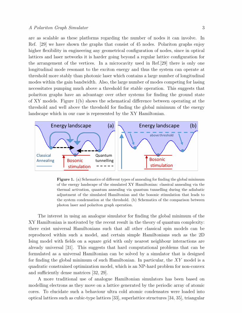
Figure 1(a) shows the schematics of the classical thermal annealing, quantum annealing
via tunnelling between the metastable states and the bosonic stimulation.
The XY model has been previously simulated by other physical systems: ultra cold
atomic optical lattices [30] and coupled photon lasers network [13]. Polariton graphs
A Polariton Graph Simulator 3
are as scalable as these platforms regarding the number of nodes it can involve. In
Ref. [29] we have shown the graphs that consist of 45 nodes. Polariton graphs enjoy
higher flexibility in engineering any geometrical configuration of nodes, since in optical
lattices and laser networks it is harder going beyond a regular lattice configuration for
the arrangement of the vertices. In a microcavity used in Ref.[29] there is only one
longitudinal mode resonant to the exciton energy and thus the system can operate at
threshold more stably than photonic laser which contains a large number of longitudinal
modes within the gain bandwidth. Also, the large number of modes competing for lasing
necessitates pumping much above a threshold for stable operation. This suggests that
polariton graphs have an advantage over other systems for finding the ground state
of XY models. Figure 1(b) shows the schematical difference between operating at the
threshold and well above the threshold for finding the global minimum of the energy
landscape which in our case is represented by the XY Hamiltonian.
Energy'landscape Energy'landscape(a) (b)
Classical'Annealing
Quantum''tunnellingBosonic
stimulationBosonicstimulation
above'threshold'
Figure 1. (a) Schematics of different types of annealing for finding the global minimum
of the energy landscape of the simulated XY Hamiltonian: classical annealing via the
thermal activation, quantum annealing via quantum tunnelling during the adiabatic
adjustment of the simulated Hamiltonian and the bosonic stimulation that leads to
the system condensation at the threshold. (b) Schematics of the comparison between
photon laser and polariton graph operation.
The interest in using an analogue simulator for finding the global minimum of the
XY Hamiltonian is motivated by the recent result in the theory of quantum complexity:
there exist universal Hamiltonians such that all other classical spin models can be
reproduced within such a model, and certain simple Hamiltonians such as the 2D
Ising model with fields on a square grid with only nearest neighbour interactions are
already universal [31]. This suggests that hard computational problems that can be
formulated as a universal Hamiltonian can be solved by a simulator that is designed
for finding the global minimum of such Hamiltonian. In particular, the XY model is a
quadratic constrained optimization model, which is an NP-hard problem for non-convex
and sufficiently dense matrices [32, 29].
A more traditional use of analogue Hamiltonian simulators has been based on
modelling electrons as they move on a lattice generated by the periodic array of atomic
cores. To elucidate such a behaviour ultra cold atomic condensates were loaded into
optical lattices such as cubic-type lattices [33], superlattice structures [34, 35], triangular

A Polariton Graph Simulator 4
[36], hexagonal [36, 37] and Kagome [38] lattices. Polariton graphs can easily produce
such or any other ordered or disordered lattice. It was recently shown that a linear
periodic chain of exciton-polariton condensates demonstrate not only various classical
regimes: ferromagnetic, antiferromagnetic and frustrated spiral phases, but also at
higher pumping intensities bring about novel exotic phases that can be associated with
spin liquids [39]. Relationship between the energy spectrum of the XY Hamiltonian and
the total number of condensed polariton particles has been established in Ref.[40] where
it was shown that “particle mass residues” of successive polariton states (defined as the
difference between the masses of the individual condensates and the total mass) that
occur with increasing excitation density above condensation threshold are an accurate
approximation of the XY Hamiltonian’s energy spectrum. Therefore, polariton graph
condensate system may represent not only the ground state but also the spectral gap of
the XY model.
Our paper is organised as follows. In Section 2 we consider the mean-field model
of polariton condensates and derive analytical solutions for a single condensate. We
establish the phase mapping of a polariton graph into the XY model in Section 3. In
Section 4 we derive the Kuramoto model that describes the dynamics of the phases of
the polariton condensates and show its relevance to the XY model. We conclude with
the discussions in Section 5.
2. An approximate analytical solution for a single condensate
The mean field of polariton condensates can be modelled [41, 42] in association with
atomic lasers by writing a driven-dissipative Gross-Pitaevskii equation (aka the complex
Ginzburg-Landau equation (cGLE)) for the condensates wavefunction ψ(r, t) :
ih∂ψ
∂t= − h2
2m(1− iηdR)∇2ψ+U0|ψ|2ψ+ hgRRψ+
ih
2(RRR− γC)ψ(1)
coupled to the rate equation for the density of the hot exciton reservoir, R(r, t):
∂R∂t
= (γR +RR|ψ|2)R+ P (r). (2)
In these equations m is polariton effective mass, U0 and gR are the strengths of effective
polariton-polariton and polariton-exciton interactions, respectively, ηd is the energy
relaxation coefficient specifying the rate at which gain decreases with increasing energy,
RR is the rate at which the reservoir excitons enter the condensate, γC is the rates of the
condensate losses, γR is the redistribution rate of reservoir excitons between the different
energy levels, and P is the pumping into the reservoir. In the limit γR � γC one can
replace Eq. 2 with the stationary state for the reservoir R = P (r)/(γR +RR|ψ|2).To non-dimensionalize the cGLE we use ψ →
√h2/2mU0`20Ψ, r→ `0r, t→ 2mt`20/h,
where we choose `0 = 1µ m and introduce the notations g = 2gR/RR, γ = mγC`20/h,
p = m`20RRP (r)/hγR, η = ηdh/mRR`20, and b = RRh
2/2m`20γRU0.
The dimensionless form of Eqs. (1)-(2) becomes the cGLE with a saturable
nonlinearity

A Polariton Graph Simulator 5
i∂Ψ
∂t= − (1− iηnR)∇2Ψ + |Ψ|2Ψ + gnRΨ + i (nR − γ) Ψ, (3)
nR = p(r)/(1 + b|Ψ|2). (4)
By taking the Taylor expansion for small |Ψ|2 in the expression for the reservoir nR
we arrive at the more standard cGLE
i∂Ψ
∂t= −(1− iηp)∇2Ψ + (1− pb)|Ψ|2Ψ + gpΨ + i
(p− γ − pb|Ψ|2
)Ψ, (5)
where, in the view of smallness of η we dropped gη|Ψ|2 term. We can compare the
relative strength of nonlinearities in Eqs. (3-4) and (5) depending of the physical
quantities that define b. By taking the values the system parameters typically accepted
for GaAs microcavities [43, 44, 26] hRR = 0.1meV·µm2, U0 = 0.02 − 0.04meV·µm2 we
obtain b = 2− 4/γRps. With γR on the order of 1ps−1 we have b of the order of the real
nonlinearity.
We consider the asymptotics and approximations of the steady state solutions for a
single radially symmetric Gaussian pumping profile p(r) = p0 exp(−σr2), where p0 is the
maximum pumping intensity and σ characterises the inverse width of the Gaussian. The
Madelung transformation Ψ =√ρ exp[iS] relates the wavefunction to density ρ = |Ψ|2
and velocity u = ∇S. Separating the real and imaginary parts of Eqs. (3-4) we arrive
at the mass continuity and the Bernoulli equations:
1
rρ
d(rρu)
dr=
p(r)
1 + bρ
(1 +
η(r(√ρ)′)′
r√ρ
− ηu2)− γ, (6)
µ = −(√ρ)′′√ρ−
(√ρ)′
r√ρ
+ u2 + ρ+p(r)
1 + bρ
(g − η
rρ
d(rρu)
dr
). (7)
Away from the pumping spot, where p(r) = 0, the velocity u = |u| is given by the
outflow wavenumber kc = const with rρr + ρ = −γρr/kc, which can be integrated to
yield ρ ∼ exp[−rγ/kc]/r. From Eq. (7) at infinity we obtain µ = k2c−γ2/4k2c . In the view
of their asymptotic behaviour the condensate density and velocity can be approximated
by
ρ(r) =a0
γr exp(γrk−1c )k−1c + ξ − γr/kc + a3r3, (8)
and
u(r) = kc tanh(lr/kc), (9)
utilizing their behaviour at the origin and infinity and introducing parameters ξ, a0, a3,
and l that define the parametric family of solutions. Their values should be found from
the governing equations via matching asymptotics, as shown below.
We neglect η in the view of its smallness and substitute the expressions for the
density, velocity and the pumping profile into Eqs. (6-7). By expanding the resulting
expressions about r = 0 and setting the term to the order O(r2) to zero we obtain the
equations that define the unknown parameters ξ, a0, a3, l and kc in terms of the system

A Polariton Graph Simulator 6
parameters g, b, γ, p0, σ. The leading order expansion of Eq. (6) and the first order
expansion of Eq. (7) fix ξ and a3 as
ξ =a0b(2l + γ)
p0 − 2l − γ, a3 = − γ3
2k2c. (10)
The expansion to O(r2) of Eq. (6) determines kc as
k2c = [4a0bl3p0(2l + γ) + 3γ2(8l3 − 12l2(p0 − γ) + (p0 − γ)2γ (11)
+ 2l(2p20 − 5p0γ + 3γ2)]/(3a0bp0σ(2l + γ)2)]
Finally, the expansions to O(r2) of Eq. (7) define the remaining parameters a0 and l
through two nonlinear equations
k2c =a0ξ
+γ2(ξ + 8)
4k2cξ+
gp0ξ
a0b+ ξ, (12)
l2 =a0γ
2
k2cξ2
+5γ4
k4cξ2− 4γ4
3k4cξ− a0bgp0γ
2
k2c (a0b+ ξ)2+
gp0σξ
a0b+ ξ. (13)
Equations (8) and (9) with the parameters defined by Eqs. (10-13) for the given system
parameters g, b, γ and the pumping parameters p0 and σ fully specify the approximate
analytical solution of Eqs. (6-7). Figure 2 shows the comparison of the approximate
analytical solutions (solid lines) given by Eqs. (8-9) and the numerical solutions (dashed
lines) of Eqs. (6-7) for b = 1.5, γ = 0.2, g = 0.5 and two sets of parameters specifying
the pumping profile (a) p0 = 5, σ = 0.2 and (b) p0 = 10, σ = 0.4. The values specifying
velocity are kc = 1.65885, l = 0.541858 for (a) and kc = 1.99239, l = 0.909976 for (b).
Both analytical density and velocity profiles are in an excellent agreement with the
numerical solutions.
-10 -5 0 5 10-2-10
1
2
3
4
5
-10 -5 0 5 10-2
0
2
4
6
8
10
Distance)(µm) Distance)(µm)
uu!
!
P P(a) (b)
Figure 2. Approximate analytical (blue lines) and numerical (black lines) solutions
for density (solid lines) and velocity (dashed lines) of Eq. (5) for the pumping
profile given by p(r) = p0 exp(−σr2) (green shaded area). The system parameters
are b = 1.5, γ = 0.2, g = 0.5 and (a) σ = 0.2, p0 = 5; (b) σ = 0.4, p0 = 10.

A Polariton Graph Simulator 7
3. Mapping of phases into the classical XY Model
In the previous section we obtained solutions of the governing equation Eq. (5) for a
single pumping Gaussian spot. Spatial light modulator can be used to pump condensates
at the vertices of a distributed graph via
p(r) =N∑i=1
pi exp[−σi|r− ri|2], (14)
where pi stands for the pumping intensity at the center of the spot at position r = ri.
In what follows we shall assume that all vertices are pumped identically, so that pi = p0,
σi = σ for all i = 1, · · ·, N . To the leading order and assuming that all condensates
are well-separated we can approximate the resulting condensate wave function, ψN ,
as ΨN(r, t) ≈ ∑Ni=1 Ψ0(|r − ri|) exp(iθi), where Ψ0 = Ψ0(r) is the solution of the
stationary Eq. (5) for a single localized radially symmetric condensate pumped by
p(r) = p0 exp(−σr2), found in the previous section
Ψ0(r) =√ρ0(r) exp
[ik2cl
log cosh(l
kcr)], (15)
where ρ0(r) is given by Eq. (8). To find the total amount of matter M we write
M =∫|ΨN |2 dr =
1
(2π)2
∫|ΨN(k)|2dk, (16)
ΨN(k) =∫
exp(−ik · r)ΨN(r) dr = Ψ0(k)N∑i=1
exp(ik · xi + iθi), (17)
where Ψ0(k) = 2π∫∞0 Ψ0(r)J0(kr)rdr and J0 is the Bessel function. The total mass
becomes
M = 2πN∫ ∞0|Ψ0|2rdr +
∑i<j
Jij cos(θi − θj), (18)
Jij =1
π
∫ ∞0|Ψ0(k)|2J0(k|ri − rj|)k dk. (19)
Since the system maximizes the total number of particles given by Eq. (18), this is
equivalent to minimising the XY Hamiltonian functional HXY = −∑ni<j Jij cos θij [29].
The main contribution to the integral defining Ψ0(k) is from k = kc, where kc is the
outflow wavevector from the pumping site fully determined by the pumping profile
[28, 29].
Figure 3 shows the density contour plots (normalised) and the spin orientations
(arrows) representing the relative phases, with the incoherent pump spots located at the
vertices. The coupling between the adjacent polariton sites can be made ferromagnetic
(Jij > 0, solid lines) or antiferromagnetic (Jij < 0, dashed lines) by either varying the
distance between the pumping spots, as illustrated in Figs. 3(a-e,g) or by changing the
pumping parameters of the individual spots as shown in Fig. 3(f). Spin configuration,
such as ferromagnetic, where all Jij > 0 [Fig. 3(a)], rhombic, where all horizontal
Jij > 0 [Fig. 3(b)], spiral 1, where all Jij < 0 [Fig. 3(c)] and spiral 2, where all
horizontal Jij < 0 [Fig. 3(d)] can be obtained by controlling independently the distance

A Polariton Graph Simulator 8
Figure 3. Theoretical prediction of classical magnetic spin configurations showing
contour plots of the normalised density and spin orientations (arrows): (a) ferromagnet,
with all Jij > 0, (b) rhomb, with all horizontal Jij > 0, (c) spiral 1, with all Jij < 0,
(d) spiral 2, with all horizontal Jij < 0, (e) defect, with a single ferromagnetic coupling
(top edge), (f) star, with Jij > 0 from central vertex to all its neighbours, (g) graph,
fully disordered system. The density contour plots show |Ψ|2, with Ψ =∑
Ψi. The
individual wave functions Ψi are analytic approximations as described in the text with
b = 1.5, g = 0.5, p0 = 3, σ = 0.2.

A Polariton Graph Simulator 9
and therefore the coupling along two directions of the lattice. In atomic optical lattices,
this can be achieved via an elliptical shaking of the lattice and the spin configurations
on Fig. 3(a-d) were demonstrated for trapped atomic condensates [30].
The ultimate advantage of polariton graphs for quantum simulations is the potential
to control both the sign and the strength of any coupling, Jij, by tuning the distance
between polariton sites, or the characteristics of the pumping spots (the intensity, p0, or
the inverse width of the Gaussian, σ) leading to more exotic phases. We illustrate
the control over an individual Jij on the seven-vertex graphs of Figs. 3(e,f). In
Figure 3(e) we utilise control over an individual Jij by tuning the distance between two
vertices and introduce a single ferromagnetic coupling (defect edge) into an otherwise
antiferromagnetic configuration. In Figure 3(f) we control the coupling of a single
polariton site (central vertex) to all its neighbours by tuning the intensity of its pumping
spot and switch them to ferromagnetic in an otherwise antiferromagnetically coupled
graph (star configuration). Finally, polariton graphs allow for fully disordered systems
to be addressed as shown in Fig. 3(g).
4. Kuramoto Model
The cGLE can be reformulated as the Kuramoto model which is a paradigm for a
spontaneous emergence of collective synchronization and that has been widely used to
understand the topological organization of real complex systems from neural networks
to power grids [45]. In this context the polariton lattice describes collective dynamics of
N coupled phase oscillators with phases θi(t), characterized by the natural frequencies
ωi which are associated with the chemical potential of individual condensates.
To show this we adopt a two-mode model that neglects the spacial variations and
represents the network of interacting polariton condensates via the radiative couplings
Jij between ith and jth condensates
iΨit = |Ψi|2Ψi +(
(g + i)p
1 + b|Ψi|2− iγ
)Ψi + i
∑j
JijΨj. (20)
We neglect the blueshift g and without loss of generality let γ = 1. For the densities
and phases of the individual condensates we obtain1
2ρi(t) =
pρi1 + bρi
− ρi +∑Jij√ρiρj cos θij
θi(t) = − ρi −∑Jij
√ρj√ρi
sin θij. (21)
The radiative coupling Jij is due to the interference of the condensates from different
pumping spots [46], and are such that Jij � ρi for any j. First, we shall assume that
the density number dynamics is faster than the phase dynamics, so that the densities
acquire the instantaneous steady state values ρi = ρ = (p − 1)/b to the leading order
in Jij. In this case we get the equations of the phase dynamics represented by the
Kuramoto model:
θi(t) = −ρ−∑Jij sin θij. (22)

A Polariton Graph Simulator 10
The equilibria of system (22) are the stationary points of the potential energy landscape
V (θ) = ρN∑i=1
θi −1
2
N∑i,j=1
Jij cos θij, (23)
so that the Kuramoto model (22) describes the gradient flow to the minima of V (θ)
and, therefore, minimizes the XY Hamiltonian.
Next, we will allow for the density variations and consider two spots only. For the
system with just two condensates we introduce the average density R = (ρ1 + ρ2)/2
and the half density difference z = (ρ1 − ρ2)/2 for which the system reduces to three
equations:
θ12 = − 2z − 2J12R√
R2 − z2sin θ12,
R = p[(R + z)Q+ + (R− z)Q−]− 2R + 2J12
√R2 − z2 cos θ12,
z = p[(R + z)Q+ − (R− z)Q−]− 2z, (24)
where we defined Q± = (1 + b(R± z))−1. Assuming that z and J12 are small compared
to R we can expand these equations in small parameters z and J12 and consider the
steady state for R, which to the leading order is R = (p − 1)/b. Eliminating z from
Eq. (24) we see that θ12 satisfies the second-order differential equation
θ12 + 2(
1− 1
p+ J12 cos θ12
)θ12 = −4
(1− 1
p
)J12 sin θ12. (25)
As the pumping increases from the threshold value of pth the oscillations between two
condensates become damped with the rate proportional to 2(
1−p−1 +Jij cos θ12
). The
relative phases lock to 0 or π difference depending on whether J12 > 0 or J12 < 0,
respectively. This again agrees with the minimization of the XY Model, which for two
pumping spots is HXY = −J12 cos θ12 with minimum at θ12 = 0 if J12 > 0 and π if
J12 < 0.
Despite many numerical and analytical studies of the Kuramoto model on complex
networks of different architectures there are many questions remain, in particular, on the
dependence of synchronization on the system size, the relaxation dynamics of the model,
the effects of time-delayed couplings and stochastic noise. In a large heterogeneous
network may exist various synchronization phase transitions. These effects as well as
the effect of other correlations between intrinsic dynamical characteristics and local
topological properties could be addressed by the polariton graph simulator.
5. Conclusions
In conclusion, we discussed polariton graphs as an analog platform for minimizing the
XY Hamiltonian and therefore emulating classical spin model with a potential of solving
computationally hard problems. We demonstrated that the search for the global ground
state of a polariton graph is equivalent to the minimisation of the XY Hamiltonian
HXY = −∑ Jij cos(θij). The theoretically predicted phase transitions explained the

A Polariton Graph Simulator 11
recent experiments for small and large scale polariton graphs [28, 26, 29]. Polariton
graphs offer the scalability of optical lattices, together with the potential to study
disordered systems and to control both the sign and the strength of the coupling for
each edge independently. Phase transitions in polariton graphs occur at the global
ground state. With the recent advances in the field of polariton condensates, such
as room temperature operation [47] and condensation under electrical pumping [48],
polariton graph based simulators offer unprecedented opportunities in addressing NP-
complete and hard problems, topological quantum information processing and the study
of exotic quantum phase transitions. Finally, we would like to emphasize that the word
”quantum” could be attached to our proposal for a simulator to reflect the statistical
nature of polariton condensates. The process of Bose-Einstein condensation is inherent
to quantum statistics where a large fraction of bosons occupies the lowest quantum
state, at which point macroscopic quantum phenomena become apparent. The use of
the classical mean-field equations to describe the kinetics of the condensate does not
negate the quantum statistic nature of its existence. At the same time, the proposed
simulator has a quantum speed-up which is associated with the stimulated process of
condensation i.e. an accelerated relaxation to the global ground quantum state.
6. References
[1] Feynman R R 1982 Simulating physics with computers Int. J. Theor. Phys. 21 467
[2] Greiner M, Mandel O, Esslinger T, Hansch T and Bloch I. 2002 Quantum phase transition from
a superfulid to a Mott insulator in a gas of ultracold atoms Nature 415 39
[3] Lewenstein M, Sanpera A, Ahufinger V, Damski B, Sen A and Sen U 2007 Ultracold atomic gases
in optical lattices: mimicking condensed matter physics and beyond Advances in Physics 56 243
[4] Saffman M, Walker T G, and Molmer K 2010 Quantum information with Rydberg atoms Rev.
Mod. Phys. 82 2313
[5] Simon J, Bakr W S, Ma R, Tai M E, Preiss Ph M and Greiner M 2011 Quantum simulation of
antiferromagnetic spin chains in an optical lattice Nature 472 307
[6] Esslinger T 2010 Fermi-Hubbard Physics with Atoms in an Optical Lattice Annu. Rev. Condens.
Matter Phys. 1 129
[7] Northup T E and Blatt R 2014 Quantum information transfer using photons Nature Photonics 8
356
[8] Kim K, Chang M-S, Korenblit S, Islam R, Edwards E E, Freericks J K, Lin G-D, Duan L-M, and
Monroe C 2010 Quantum simulation of frustrated Ising spins with trapped ions Nature 465 590
[9] Lanyon B P, Hempel C, Nigg D, Muller M, Gerritsma R, Zuhringer F, Schindler P, Barreiro J
T, Rambach M, Kirchmair G, Hennrich M, Zoller P, Blatt R, Roos C F 2011 Universal digital
quantum simulation with trapped ions Science 334 57
[10] Corcoles A D, Magesan E, Srinivasan S J, Cross A W, Steffen M, Gambetta J M and Chow J M 2015
Demonstration of a quantum error detection code using a square lattice of four superconducting
qubits, Nature Commun. 6 6979
[11] Utsunomiya S, Takata K and Yamamoto Y 2011 Mapping of Ising models onto injection-locked
laser systems, Opt. Express 19 18091
[12] Marandi A, Wang Z, Takata K, Byer R L, and Yamamoto Y, Network of time-multiplexed optical
parametric oscillators as a coherent Ising machine Nature Photonics 8 937
[13] Nixon M, Ronen E, Friesem A A, and Davidson N 2013 Observing geometric frustration with
thousands of coupled lasers Phys. Rev. Lett. 110 184102

A Polariton Graph Simulator 12
[14] Bloch I, Dalibard J and Nascimbene S 2012 Quantum simulations with ultracold quantum gases
Nature Physics 8 267
[15] Weisbuch C, Nishioka M, Ishikawa A and Arakawa, Y 1992 Observation of the coupled exciton-
photon mode splitting in a semiconductor quantum microcavity. Phys. Rev. Lett. 69 3314
[16] Kasprzak J et al. 2006 Bose-Einstein condensation of exciton polaritons Nature 443 409
[17] Deng H, Weihs G, Santori C, Bloch J and Yamamoto Y 2002 Condensation of Semiconductor
Microcavity Exciton Polaritons Science 298 199
[18] Keeling J and Berloff N G 2011 Exciton-polariton condensation Contemporary Physics 52 131
[19] Carusotto I and Ciuti C 2013 Quantum Fluids of Light Rev. Mod. Phys. 85 299
[20] Nardin G, Leger Y, Pietka B, Morier-Genoud F, Deveaud-Pledran B 2010 Phase-resolved imaging
of confined exciton-polariton wave functions in elliptical traps Phys. Rev. B 82 045304
[21] Galbiati M et al 2012 Polariton Condensation in Photonic Molecules Phys. Rev. Lett. 108 126403
[22] Lai C W et al 2007 Coherent zero-state and p-state in an exciton-polariton condensate array Nature
450 529
[23] Balili R, Hartwell V, Snoke D, Pfeiffer L and West K 2007 Bose-Einstein Condensation of
Microcavity Polaritons in a Trap Science 316 1007
[24] Miller D A B, Chemla D S, Damen T C, Gossard A C, Wiegmann W, Wood T H, Burrus C A
1984 Band-Edge Electroabsorption in QuantumWell Structures: The Quantum-Confined Stark
Effect Phys. Rev. Lett. 53 2173
[25] Keeling J and Berloff N G 2011 Controllable half-vortex lattices in an incoherently pumped
polariton condensate arXiv:1102.5302
[26] Tosi G, Christmann G, Berloff N G, Tsotsis P, Gao T, Hatzopoulos Z, Savvidis P G and Baumberg
J J 2012 Sculpting oscillators with light within a nonlinear quantum fluid Nature Physics 8 190
[27] Tosi G, Christmann G, Berloff N G, Tsotsis P, Gao T, Hatzopoulos Z, Savvidis P G and Baumberg
J J 2013 Geometrically locked vortex lattices in semiconductor quantum fluids Nature Comm 3
1243
[28] Ohadi H, Gregory R L, Freegarde T, Rubo Y G, Kavokin A V, Berloff N G and Lagoudakis P G
2016 Nontrivial Phase Coupling in Polariton Multiplets, Phys. Rev. X 6 031032
[29] Berloff N G, Silva M, Kalinin K, Askitopoulos A, Topfer J D, Cilibrizzi P, Langbein W and
Lagoudakis P G 2017 Realizing the classical XY Hamiltonian in polariton simulators to appear
Nature Materials, also arXiv:1607.06065
[30] Struck J et al 2011 Quantum simulation of frustrated classical magnetism in triangular optical
lattices, Science 333 996
[31] Cuevas G D and Cubitt T S 2016 Simple universal models capture all classical spin physics. Science
351 1180
[32] Pardalos P M and Vavasis S A 1991 Quadratic programming with one negative eigenvalue is
NP-hard J.Global Optim. 1 15
[33] Greiner M, Bloch I, Mandel M O, Hansch T W and Esslinger T 2001 Exploring phase coherence
in a 2D lattice of Bose-Einstein condensates Phys. Rev. Lett. 87 160405
[34] Sebby-Strabley J, Anderlini M, Jessen P and Porto J 2006 Lattice of double wells for manipulating
pairs of cold atoms Phys. Rev. A 73 033605
[35] Folling S et al 2007 Direct observation of second-order atom tunnelling Nature 448 1029
[36] Becker C et al 2010 Ultracold quantum gases in triangular optical lattices New J. Phys. 12 065025
[37] Tarruell L, Greif D, Uehlinger T, Jotzu G and Esslinger T 2012 Creating, moving and merging
Dirac points with a Fermi gas in a tunable honeycomb lattice Nature 483 302
[38] Jo G-B et al 2011 Ultracold atoms in a tunable optical kagome lattice Phys. Rev. Lett. 108 045305
[39] Kalinin K, Lagoudakis P G and Berloff N G 2017 Exotic states of matter with polariton chains,
in review by Phys. Rev. Letts. (2017)
[40] Exotic states of matter with polariton chains, in review by Phys. Rev. Letts. (2017)
[41] Wouters M and Carusotto I 2007 Excitations in a nonequilibrium Bose-Einstein condensate of
exciton polaritons, Phys. Rev. Lett. 99 140402
A Polariton Graph Simulator 13
[42] Keeling J and Berloff N G 2008 Spontaneous rotating vortex lattices in a pumped decaying
condensate Phys. Rev. Lett. 100 250401
[43] Manni F, Lagoudakis K G, Liew T C H, Andre R and Deveaud-Pledran B 2011 Spontaneous
pattern formation in a polariton condensate Phys. Rev. Lett. 107 106401
[44] Lagoudakis K G et al 2008 Quantized vortices in an exciton?polariton condensate Nat. Phys. 4
706
[45] Rodrigues F A, Peron T K, Ji P and Kurths J 2016 The Kuramoto model in complex networks
Physics Reports, 610 1
[46] Aleiner I L, Altshuler B L and Rubo Y G 2012 Radiative coupling and weak lasing of exciton-
polariton condensates Phys. Rev. B 85 121301(R)
resulting from finite inertia in coupled oscillator systems Phys. Rev. Letts. 78 2104
oscillators with hysteretic responses Physica D: Nonlinear Phenomena 100 279 13 R135 (2001)
[47] Plumhof J D, Stoferle T, Mai L, Scherf U and Mahrt R F 2014 Room-temperature Bose-Einstein
condensation of cavity exciton-polaritons in a polymer Nat. Mat. 13 247
[48] Schneider C et al 2013 An electrically pumped polariton laser Nature 497 348