VILNIUS UNIVERSITY

PAVEL STEFANOVIČ

VISUALIZATION OF SELF-ORGANIZING MAPS AND ESTIMATION OF THEIR

QUALITY

Summary of Doctoral Dissertation

Physical Sciences, Informatics (09 P)

Vilnius, 2015

The doctoral dissertation was prepared at the Institute of Mathematics and Informatics of

Vilnius University in 2010-2014.

Scientific Supervisor

Assoc. Prof. Dr. Olga Kurasova (Vilnius University, Physical Sciences, Informatics –

09 P).

The dissertation will be defended at the Council of the Scientific Field of Informatics

of Vilnius University:

Chairman

Prof. Habil. Dr. Antanas Žilinskas (Vilnius University, Physical Sciences,

Informatics – 09 P).

Members:

Prof. Habil. Dr. Kazys Kazlauskas (Vilnius University, Physical Sciences,

Informatics – 09 P),

Assoc. Prof. Dr. Raimundas Matulevičius (University of Tartu, Physical Sciences,

Informatics – 09 P),

Prof. Dr. Dalius Navakauskas (Vilnius Gediminas Technical University,

Technological Sciences, Informatics Engineering – 07 T),

Prof. Dr. Rimantas Vaicekauskas (Vilnius University, Physical Sciences,

Informatics – 09 P).

The dissertation will be defended at the public meeting of the Council of the Scientific

Field of Informatics Sciences of Vilnius University in the auditorium number 203 at the

Institute of Mathematics and Informatics of Vilnius University at 11 a. m. on the 30th of

June 2015.

Address: Akademijos st. 4, LT-08663 Vilnius, Lithuania.

The summary of the doctoral dissertation was sent out on 29th of May 2015.

A copy of the doctoral dissertation is available for review at the Library of Vilnius

University or on this website: www.vu.lt/lt/naujienos/ivykiu-kalendorius

VILNIAUS UNIVERSITETAS

PAVEL STEFANOVIČ

SAVIORGANIZUOJANČIŲ NEURONINIŲ TINKLŲ VIZUALIZAVIMAS IR JO

KOKYBĖS NUSTATYMAS

Daktaro disertacija,

Fiziniai mokslai, informatika (09 P)

Vilnius, 2015

Disertacija rengta 2010–2014 metais Vilniaus universiteto Matematikos ir informatikos

institute.

Mokslinė vadovė

doc. dr. Olga Kurasova (Vilniaus universitetas, fiziniai mokslai, informatika – 09 P).

Disertacija ginama Vilniaus universiteto Informatikos mokslo krypties taryboje:

Pirmininkas

prof. habil. dr. Antanas Žilinskas (Vilniaus universitetas, fiziniai mokslai,

informatika – 09 P).

Nariai:

prof. habil. dr. Kazys Kazlauskas (Vilniaus universitetas, fiziniai mokslai,

informatika – 09 P),

doc. dr. Raimundas Matulevičius (Tartu universitetas, fiziniai mokslai,

informatika – 09 P),

prof. dr. Dalius Navakauskas (Vilniaus Gedimino technikos universitetas,

technologijos mokslai, informatikos inžinerija – 07 T),

prof. dr. Rimantas Vaicekauskas (Vilniaus universitetas, fiziniai mokslai,

informatika – 09 P).

Disertacija bus ginama viešame Vilniaus universiteto Informatikos mokslo krypties

tarybos posėdyje 2015 m. birželio 30 d. 11 val. Vilniaus universiteto Matematikos ir

informatikos instituto 203 auditorijoje.

Adresas: Akademijos g. 4, LT-08663 Vilnius, Lietuva.

Disertacijos santrauka išsiuntinėta 2015 m. gegužės 29 d.

Disertaciją galima peržiūrėti Vilniaus universiteto bibliotekoje ir VU interneto svetainėje

adresu: www.vu.lt/lt/naujienos/ivykiu-kalendorius

5

1. Introduction

1.1. Research area and relevance of the problem

Nowadays technologies allow us to accumulate large amounts of different information and

save it in the computer memory, external media or on the Internet. In the course of time,

collection and storage become a load of rubbish which often makes it difficult to find the

required data and other useful information. Modern technology enables us to quickly find

a big amount of information about one or other thing you want, but the information found

is often useless, distorted, and irrelevant. Therefore, it is becoming a serious problem and

a challenge for every user. One of the solutions to solve this problem is data mining

methods, which allow us to structure data by clustering, classifying them and, if there is a

possibility, presenting the results visually.

One of the data mining methods is self-organizing networks. Usually this data mining

method is called a self-organizing map (SOM), and sometimes by the name of the creator

the Kohonen map. SOM can be used to cluster and visualize multidimensional data, as

well as find the multidimensional data projection into a smaller number of dimensions of

space. Despite that more than 40 years have passed after the appearance of SOM, it is still

intensively researched and applied. Over time, a lot of various extensions and

modifications of SOM have appeared, starting from the learning rules for different ways

of SOM visualization techniques, but the main principle of the original self-organizing

map remains the same. For many years, SOM has been applied to clustering and

classifying of the numerical data, but currently, the scope of investigation has extended to

the analysis of the textual data or other type of data.

One of SOM advantages as compared with other data mining methods is that, as a

result SOM gives not only numerical estimates, like most other data mining methods, but

the also results are presented in a visual form, and the visual information enables a user to

understand it faster than the textual or numerical information. Mostly SOM is used to

cluster the datasets. Comparing SOM with other clustering methods, there are no precisely

defined clusters, i. e. the data are not unambiguously assigned to one or other cluster.

Clustering of results can be variously interpreted by researchers, when watching a visual

image of SOM. It allows us to notice the similarity between the data and groups that are

not known in advance, which can be an advantage over other clustering methods. SOM

6

also can be applied to data, assigned to different classes. In this case, a researcher can

investigate how classes match up to the clusters obtained in SOM, and explain the reasons

for such differences, one of which may be related to the fact that the data were incorrectly

assigned to classes.

Currently, there is a variety of software systems, that implement the SOM

visualization techniques, but there is a lack of systems in which SOM shows the number

of data in each cell of SOM and what class of data is assigned to each cell of SOM. Also,

the problem is that there are no numerical estimates showing data classes and SOM

clustering overlaps.

In addition, the SOM result highly depends on a variety of learning parameters, so

there is a problem, which values of a parameter should be chosen for analyzed datasets. It

is also important to investigate which learning parameters allow us to get more accurate

results when analyzing different types of data: textual and numerical.

So, the dissertation deals with two major problems:

1. Visualization of data, assigned to a specific class by self-organizing maps and

estimation of the obtained results.

2. Dependence of the results obtained by the self-organizing maps on learning

parameters.

1.2. Research object

The object of dissertation is data clustering, classification and visualization using self-

organizing maps and estimation of their quality

1.3. The Aim and Tasks of the Research

The aim of this work is to propose a new visualization technique of self-organizing maps,

which allows us to visualize textual and numerical data as classes are known in advance,

and to observe the coincidence of the obtained clusters and data classes, as well to propose

and investigate errors evaluating the coincidence.

To realize the aim of research, it is necessary to solve the following tasks:

1. To perform an analytical review of the existing SOM visualization techniques.

2. To propose errors, in order to evaluate the coincidence of the obtained SOM

clusters and data classes.

7

3. To propose a SOM visualization technique, with a view to investigate the data

when classes are known in advance.

4. To create a software system in which the proposed SOM visualization

technique and proposed errors to evaluate the obtained SOM quality would be

implemented.

5. To investigate experimentally the proposed SOM visualization technique and

errors, depending on the values of the selected SOM learning parameters,

analyzing the numerical and textual data.

1.4. Scientific novelty

1. The new SOM visualization technique is proposed, allowing us to see the ratio

between different members of both textual and numerical data classes in the

same SOM cell.

2. Two errors are proposed for estimation the SOM quality, which are suitable

for data when their classes are known in advance.

3. It is investigated how different factors of text document conversion to

numerical expression influence the SOM results obtained.

1.5. The defended statements

1. The proposed SOM visualization technique allows us to see the ratio between

different data class members in the same SOM cell for both textual and

numerical datasets.

2. The proposed errors for estimating the SOM quality allows us to estimate the

coincidence between data classes and clusters obtained by SOM.

3. The appropriate of selected factors conversion of text documents into a

numerical expression improve the results obtained by SOM.

1.6. The practical value of the study results

The new SOM system has been developed. Not only the proposed SOM visualization

technique and errors to estimate the SOM quality are implemented in the new SOM

system, but also there is a possibility to choose various neighboring functions and learning

rates, which values can be changed in each iteration or epoch. It is also possible to split

the analyzed dataset into two subsets: training and testing. For this reason, the new SOM

8

system can be used not only to analyze the data, but also to investigate the SOM features.

A part of the research results has been supported by the project ’Theoretical and

engineering aspects of e-service technology development and application in high-

performance computing platforms’ (No. VP1-3.1-SMM-08-K-01-010) funded by the

European Social Fund.

1.7. Approbation and Publications of the Research

The main results of the dissertation were published in 7 scientific publications: five are

published in periodicals, reviewed scientific journals, two of them are refereed in the

‘Thomson Reuters Web of Science’ database with an impact factor; other two publications

are published in conference proceedings. Besides two abstracts were published in

international conference abstracts proceedings. The main results of the work have been

presented and discussed at 4 national and 3 international conferences.

1.8. Outline of the Dissertation

The dissertation consists of 5 chapters and references. The chapters of the dissertation are

as follows: ‘Introduction’, ‘Review of self-organizing maps’, ‘The proposed errors for

estimation of SOM quality’, ‘The experimental results’, ‘Summary’, and ‘General

Conclusions’. The dissertation also includes the list of notation and abbreviations. The

scope of the work is 132 pages that include 49 figures and 27 tables. The list of references

consists of 87 sources.

2. Review of self-organizing maps

T. Kohonen began to explore self-organizing maps (SOMs) in 1982. More than 30 years

have passed since that time, but SOM does not lose its popularity. New extensions and

modifications are developed constantly. The main target of SOM is to preserve the

topology of multidimensional data, i. e., to get a new set of data from the input data such

that the new set preserved the structure (clusters, relationships, etc.) of the input data

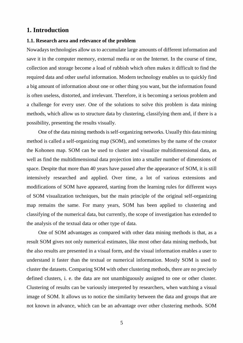
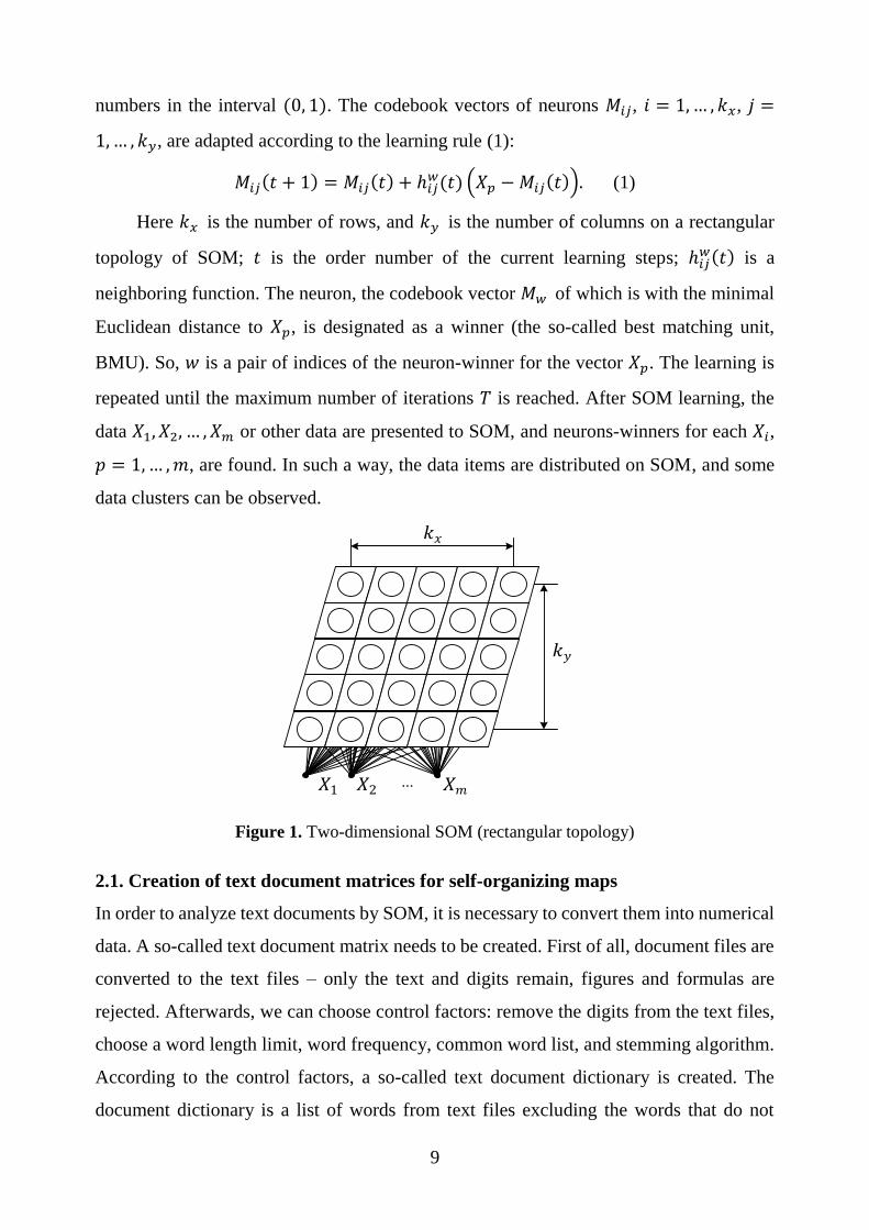
(Kohonen, 2001). SOM is applied to cluster and visualize data. The self-organizing map

is a set of nodes, connected to one another via a rectangular or hexagonal topology. The

rectangular topology of SOM is presented in Figure 1. The learning starts from setting the

initial values of components of the codebook vectors 𝑀𝑖𝑗. Usually these values are random

9

numbers in the interval (0, 1). The codebook vectors of neurons 𝑀𝑖𝑗, 𝑖 = 1, … , 𝑘𝑥, 𝑗 =

1, … , 𝑘𝑦, are adapted according to the learning rule (1):

𝑀𝑖𝑗(𝑡 + 1) = 𝑀𝑖𝑗(𝑡) + ℎ𝑖𝑗𝑤(𝑡) (𝑋𝑝 − 𝑀𝑖𝑗(𝑡)). (1)

Here 𝑘𝑥 is the number of rows, and 𝑘𝑦 is the number of columns on a rectangular

topology of SOM; 𝑡 is the order number of the current learning steps; ℎ𝑖𝑗𝑤(𝑡) is a

neighboring function. The neuron, the codebook vector 𝑀𝑤 of which is with the minimal

Euclidean distance to 𝑋𝑝, is designated as a winner (the so-called best matching unit,

BMU). So, 𝑤 is a pair of indices of the neuron-winner for the vector 𝑋𝑝. The learning is

repeated until the maximum number of iterations 𝑇 is reached. After SOM learning, the

data 𝑋1, 𝑋2, … , 𝑋𝑚 or other data are presented to SOM, and neurons-winners for each 𝑋𝑖,

𝑝 = 1, … , 𝑚, are found. In such a way, the data items are distributed on SOM, and some

data clusters can be observed.

...𝑋2 𝑋𝑚

𝑘𝑥

𝑘𝑦

𝑋1

Figure 1. Two-dimensional SOM (rectangular topology)

2.1. Creation of text document matrices for self-organizing maps

In order to analyze text documents by SOM, it is necessary to convert them into numerical

data. A so-called text document matrix needs to be created. First of all, document files are

converted to the text files – only the text and digits remain, figures and formulas are

rejected. Afterwards, we can choose control factors: remove the digits from the text files,

choose a word length limit, word frequency, common word list, and stemming algorithm.

According to the control factors, a so-called text document dictionary is created. The

document dictionary is a list of words from text files excluding the words that do not

10

satisfy the conditions defined by the control factors. Descriptions of the control factors,

when a document dictionary is being created, are as follows:

Almost in all text documents, there are digits. There is no need to include them

into the document dictionary, because they do not characterize the text

document.

The word length limit is the number indicating the smallest length of words

which will be included into the document dictionary. It is not advisable to

include short words, such as the author’s initials, articles ‘a’, ‘an’, ‘the’, or other

not informative words into the dictionary.

The common word list is a list of words that will not be included into the

document dictionary. Often the words such as ‘there’, ‘where’, ‘that’, ‘when’,

etc. compose the common word list. All of them are not important for document

analysis, so these words just distort the results. However, the common word list

can depend on the domain of text documents. For example, if we analyze

scientific papers, the words such as ‘describe’, ‘present’, ‘new’, ‘propose’,

‘method’, etc. also do not characterize the papers and it is not purposeful to

include them into the document dictionary.

The stemming algorithm separates the stem from the word (Porter, 1980). For

example, we have four words ‘accepted’, ‘acceptation’, ‘acceptance’, and

‘acceptably’. The stem of the words is ‘accept’. Only it is included into the

document dictionary. All the other words are ignored.

The word frequency is the number indicating how many times the word has to

be repeated in the text so that it could be included into the dictionary. If a small

frequency is chosen, rare words that do not characterize the text document will

be included into the document dictionary. Otherwise, if a large frequency is

chosen, frequent words will be included into the document dictionary, but not

all of them characterize the text document.

Thus, the proper values of these control factors should be chosen in order to get a

dictionary that characterizes the text documents as exactly as possible. According to the

frequency of the document dictionary words in the text documents, a so-called text

document matrix is created (2).

11

(

𝑥11 𝑥12 … 𝑥1𝑛

𝑥21 𝑥22 … 𝑥2𝑛

⋮ ⋮ ⋱ ⋮𝑥𝑚1 𝑥𝑚2 … 𝑥𝑚𝑛

) (2)

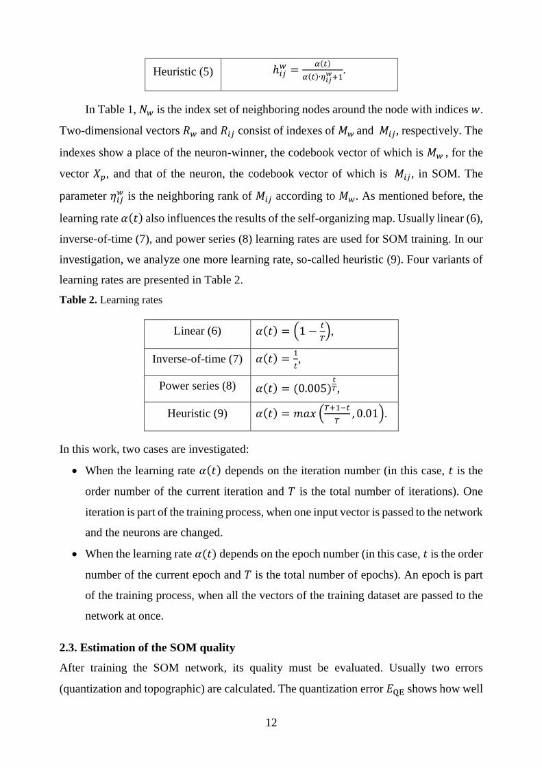
Here 𝑥𝑝𝑙 is the frequency of the 𝑙th word in the 𝑝th text document, 𝑝 = 1, … , 𝑚, 𝑙 =

1, … , 𝑛. 𝑚 is the number of the analyzed text documents, and 𝑛 is the number of words in

the text document dictionary. Therefore, the document matrix is a matrix the elements of

which are equal to frequencies of the document dictionary words in the text documents. A

row of matrix (2) is a vector, corresponding to a document. These vectors 𝑋1, 𝑋2, … , 𝑋𝑚

can be used for training SOM, 𝑋𝑝 = (𝑥𝑝1, 𝑥𝑝2, … , 𝑥𝑝𝑛), 𝑝 = 1, … , 𝑚. They are presented

to SOM as input vectors. A set of the vectors 𝑋1, 𝑋2, … , 𝑋𝑚 composes a dataset analyzed.

A data item corresponds to a vector, 𝑛 is a dimensionality of the data item.

Over the past decade, many researches dealing with text mining have been

conducted. For this reason, various tools have been created to help analyze the textual data.

We use the Text to Matrix Generator (TMG) toolbox implemented in Matlab (Zeimpekis,

Gallopoulos, 2005) to create text document matrices. The toolbox allows us to construct

text document matrices from text documents and to perform various data mining tasks:

dimensionality reduction, clustering, classification, etc.

2.2. Learning parameters

The results of a self-organizing map depend on the selected learning parameters. Thus, it

is important to choose the best learning parameters to get better results. The results are

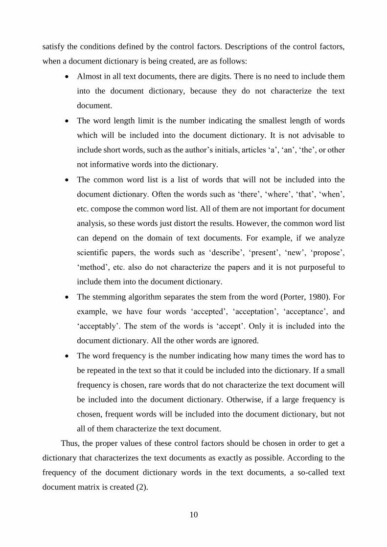
mostly affected by different neighboring functions ℎ𝑖𝑗𝑤 (Table 1) and learning rates 𝛼(𝑡)

(Table 2). Usually, two neighboring functions – bubble (3) and Gaussian (4) are used. In

our research, we analyze one more neighboring function, so-called heuristic (5) (Dzemyda,

2001).

Table 1. Neighboring functions

Bubble (3) ℎ𝑖𝑗𝑤(𝑡) = {

𝛼(𝑡), (𝑖, 𝑗) ∈ 𝑁𝑤

0, (𝑖, 𝑗) ∈ 𝑁𝑤,

Gaussian (4) ℎ𝑖𝑗𝑤(𝑡) = 𝛼(𝑡) ∙ exp (

−‖𝑅𝑤−𝑅𝑖𝑗‖2

2(𝜂𝑖𝑗𝑤(𝑡))

2 ),

12

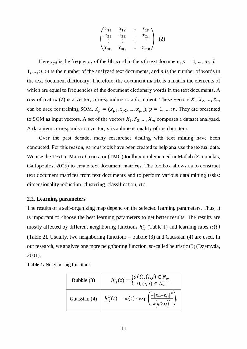
Heuristic (5) ℎ𝑖𝑗𝑤 =

𝛼(𝑡)

𝛼(𝑡)∙𝜂𝑖𝑗𝑤+1

.

In Table 1, 𝑁𝑤 is the index set of neighboring nodes around the node with indices 𝑤.

Two-dimensional vectors 𝑅𝑤 and 𝑅𝑖𝑗 consist of indexes of 𝑀𝑤 and 𝑀𝑖𝑗, respectively. The

indexes show a place of the neuron-winner, the codebook vector of which is 𝑀𝑤 , for the

vector 𝑋𝑝, and that of the neuron, the codebook vector of which is 𝑀𝑖𝑗, in SOM. The

parameter 𝜂𝑖𝑗𝑤 is the neighboring rank of 𝑀𝑖𝑗 according to 𝑀𝑤. As mentioned before, the

learning rate 𝛼(𝑡) also influences the results of the self-organizing map. Usually linear (6),

inverse-of-time (7), and power series (8) learning rates are used for SOM training. In our

investigation, we analyze one more learning rate, so-called heuristic (9). Four variants of

learning rates are presented in Table 2.

Table 2. Learning rates

Linear (6) 𝛼(𝑡) = (1 −𝑡

𝑇),

Inverse-of-time (7) 𝛼(𝑡) =1

𝑡,

Power series (8) 𝛼(𝑡) = (0.005)𝑡

𝑇,

Heuristic (9) 𝛼(𝑡) = 𝑚𝑎𝑥 (𝑇+1−𝑡

𝑇, 0.01).

In this work, two cases are investigated:

When the learning rate 𝛼(𝑡) depends on the iteration number (in this case, 𝑡 is the

order number of the current iteration and 𝑇 is the total number of iterations). One

iteration is part of the training process, when one input vector is passed to the network

and the neurons are changed.

When the learning rate 𝛼(𝑡) depends on the epoch number (in this case, 𝑡 is the order

number of the current epoch and 𝑇 is the total number of epochs). An epoch is part

of the training process, when all the vectors of the training dataset are passed to the

network at once.

2.3. Estimation of the SOM quality

After training the SOM network, its quality must be evaluated. Usually two errors

(quantization and topographic) are calculated. The quantization error 𝐸QE shows how well

13

neurons of the trained network adapt to the input vectors. Quantization error (10) is the

average distance between the data vectors 𝑋𝑝 and their neuron-winners 𝑀𝑤(𝑝).

Topographic error 𝐸𝑇𝐸 shows how well the trained network keeps the topography of

the data analyzed. The topographic error (11) is calculated by the formula:

If the neuron-winner of vector 𝑋𝑝 is near to the neuron, the distance from 𝑋𝑝 to it is the

smallest one, disregarding the neuron-winner, then 𝑢(𝑋𝑝) = 0, otherwise, 𝑢(𝑋𝑝) = 1.

2.4. Extensions and modification of self-organizing maps

More than 30 years have passed since the self-organizing maps has been introduced, so

the new extensions and modifications are developed constantly. In the dissertation a

review of commonly used SOM modifications and extensions is presented, namely: merge

self-organizing map (Strickert, Hammer, 2005), recursive self-organizing map (Voegtlin,

2002), WEBSOM (Kaski and other, 1998), etc. Mostly all of them are created to speed-up

the learning algorithm or to perform specific tasks. For example, WEBSOM is the first

SOM extension created for the textual document analysis.

Now a lot of researchers are still using SOM for different problem solutions. One of

the newest SOM modifications is the batch-learning self-organizing map (BLSOM), used

in the bioinformatics area (Iwasaki, 2013). In this method, SOM has been modified for

gene informatics to make the learning process and resulting map independent of the data

input. BLSOM is a powerful tool for big data analysis. It allows us to visualize and classify

big sequences, obtained from genomes (millions of metagenomics sequences).

Also, we can find SOM extensions with an unusual visualization technique suitable

for unstructured data. This visualization technique (Prakash, 2013) helps us to analyze

several features at once, so it is much more suitable for a big data visual analysis. As a

result, we get SOM as a spider graph, where we can find a large number of analyzed

features in each graph.

𝐸QE =1

𝑚∑ ‖𝑋𝑝 − 𝑀𝑤(𝑝)‖𝑚

𝑝=1 . (10)

𝐸TE =1

𝑚∑ 𝑢(𝑋𝑝)𝑚

𝑝=1 . (11)

14

2.5. Self-organizing map systems

In the dissertation an analytical overview of the most popular SOM systems is made. In

order to demonstrate visualization techniques, implemented into SOM systems (SOM-

Toolbox, Databionic ESOM, Viscovery SOMine, NeNet), experiments have been carried

out using two datasets and these systems. Other SOM systems have also been reviewed,

such as: Orange, SOM-analyzer, R package for SOM and others. In the review, the

advantages and disadvantages of systems are highlighted.

One of the main disadvantages of all the reviewed systems is that there is no

possibility to see the number of all vectors which fall in the same cell of SOM. It is

important, because only showing a single class member in the cell, it is not clear how many

and which class members are in the same cell of SOM, so the researcher cannot say which

SOM cluster obtained is ‘stronger’. It is also purposeful to propose new errors that would

enable to estimate the SOM quality considering the coincidence of data classes and clusters

obtained in SOM.

3. The proposed errors for estimation of SOM quality

As mentioned before, after training SOM, usually the quantization 𝐸QE and topographic

𝐸TE errors are calculated. However, these two errors do not show whether the analyzed

dataset classes correspond to the clusters formed in the SOM. Often, when we analyze the

classified data by the clustering methods, there is a need to evaluate the coincidence

between data classes and the obtained clusters. The coincidence indicates that the data are

assigned to appropriate classes. In a mismatch case, the researcher must to seek causes of

the data mismatch. One of the possible reason is that the data are assigned to unsuitable

classes. There are some errors, that help evaluate the coincidences between classes and the

obtained clusters (Manning and others, 2008), but then the data must be unambiguously

assigned to one of the clusters. SOM uniqueness, comparing with other clustering methods

is that in the SOM results there is no strictly expressed cluster, i. e. it is not specified which

data item is assigned to which cluster, only the formed clusters we can usually see in the

SOM. The researcher, observing the maps, can see and estimate the coincidence (and

mismatch) of data classes and clusters. The problem arises when you have to view and

explore a lot of SOM maps. As it is known, the SOM results can depend on different

learning parameters and factors of the text document conversion into numerical

15

expression, – various factors yield different SOM results. Therefore, the researcher has to

view many SOM maps. Furthermore, there may be cases where the visual differences

between the results (coincidences of classes and clusters) are not obvious, so it is very

difficult to determine in which SOM the clusters are far from one other, and in which they

are close to each other. For these reasons, in the dissertation two new heuristic errors are

proposed to estimate the SOM quality when the classified data are analyzed. The proposed

errors can be applied to compare several SOM maps, that are analyzing the same dataset

and SOM sizes are the same.

3.1. The first proposed error – evaluation of the same class members

If we analyze the data when classes are known in advance, it is important to verify how

the data of the same class are located in SOM. Thus, the first proposed error estimates how

close the same class members are in SOM and the SOM clusters coincide. It allows us to

estimate if all the data from the same class are similar to one other. The error value is

calculated for each class separately. The proposed error 𝐸𝑐 is calculated by the following

formula:

𝐸𝑐 =1

𝑁𝑐∑ ∑ (‖𝑍𝑖

𝑐 − 𝑍𝑗𝑐‖𝑘𝑖

𝑐𝑘𝑗𝑐 + 𝑏𝑖𝑗)

𝑛𝑐𝑗=𝑖+1

𝑛𝑐−1𝑖=1 . (12)

Here 𝑐 is a class label; 𝑁𝑐 is the number of data items from the 𝑐th class; 𝑛𝑐 is the

total number of neurons (cells) corresponding to the data from the 𝑐th class; 𝑍𝑖𝑐 is a vector,

consisting of indices of the SOM cells, corresponding to the data from the 𝑐th class, 𝑍𝑖𝑐 ∈

𝑅2; 𝑘𝑖𝑐 is the number of the data items from the 𝑐th class in the SOM cell, the indices of

which are 𝑍𝑖𝑐. There may be cases, where the members of different classes fall into the

same SOM cell. In such a case, the penalty 𝑏𝑖𝑗 is calculated by formula (13). The penalty

is used in formula (14). If only the same class members are in one SOM cell, the penalty

is equal to 𝑏𝑖𝑗 = 0.

𝑏𝑖𝑗 =𝑙𝑖

𝑐′

𝑘𝑖+

𝑙𝑗𝑐′

𝑘𝑗. (13)

Here 𝑘𝑖 (𝑘𝑗) is the number of data vectors, that are in the cell with the indices 𝑍𝑖𝑐

(𝑍𝑗𝑐). 𝑙𝑖

𝑐′ (𝑙𝑗

𝑐′) is the number of data vectors from another class than of the cth vectors, in

the cell with the indices 𝑍𝑖𝑐 (𝑍𝑗

𝑐).

16

Purposefully, the sum of errors in (12) is not divided by the number of sum members

𝑛𝑐(𝑛𝑐 − 1)/2, because such a division unifies the results of errors if we compare several

SOMs. If data vectors of the same class are more widely distributed in the SOM, the

number 𝑛𝑐 is larger than that where the data vectors are grouped in one place. Therefore,

when we evaluate the results of several SOMs it is purposeful to divide the proposed error

by the same number, for example, by the number 𝑁𝑐 of the cth class data vectors.

The smaller value of the error 𝐸𝑐 means that the data from the same class are clustered

better on SOM. In that case, it can be said that the SOM cluster is coincident with the data

class. Thus, the researcher can not only assess the coincidence between clusters and classes

visually, but also observe the values of errors.

3.2 Second proposed error – evaluation of class centers

The first error is calculated for each class separately. However, it is also important to

evaluate how far or close the data clusters are, which correspond to the analyzed data from

the same classes in SOM. So, the second proposed error evaluates how far the different

class centers are in SOM. Observing the value of this error together with the first error

values, the researcher cannot only visually assess the coincidence of the SOM clusters and

data classes. First of all, the indices of data centers 𝑌𝑐 of each class on SOM have to be

found:

𝑌𝑐 =1

𝑛𝑐∑ 𝑍𝑖

𝑐𝑛𝑐𝑖=1 . (14)

Here 𝑛𝑐 is the total number of neurons (cells) corresponding to the data from the 𝑐th

class; 𝑍𝑖𝑐 is a vector that consists of indices of the SOM cells, corresponding to the data

from the 𝑐th class, 𝑍𝑖𝑐 ∈ 𝑅2. Then the value of the error 𝐸center is calculated by the

formula:

𝐸center =1

𝑚′∑ ∑ ‖𝑌𝑐 − 𝑌𝑑‖𝑘

𝑑=𝑐+1𝑘−1𝑐=1 . (15)

Here 𝑚′ =𝑘(𝑘−1)

2, 𝑘 is the number of data classes.

The higher value of the error 𝐸center means that the centers of classes in SOM are more

separated from one other than in the case of a lower error. The larger value of the error

means better results (the distance between different class centers is larger).

17

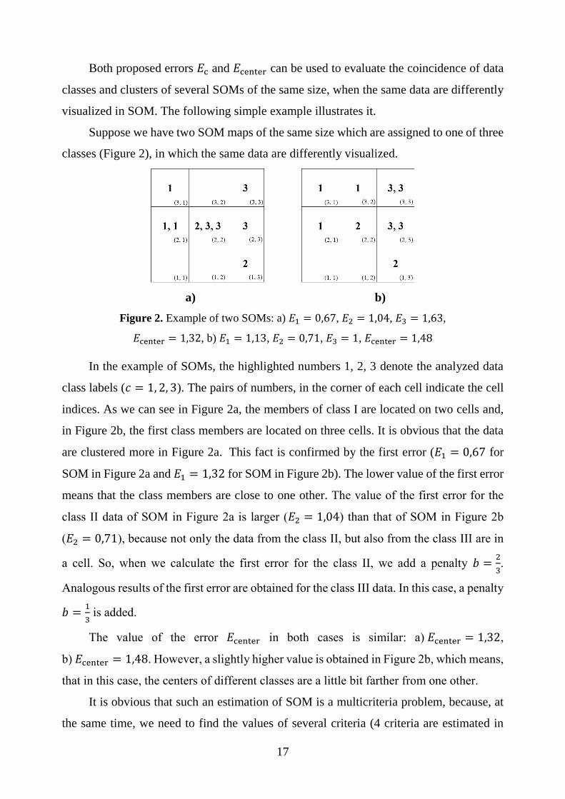
Both proposed errors 𝐸c and 𝐸center can be used to evaluate the coincidence of data

classes and clusters of several SOMs of the same size, when the same data are differently

visualized in SOM. The following simple example illustrates it.

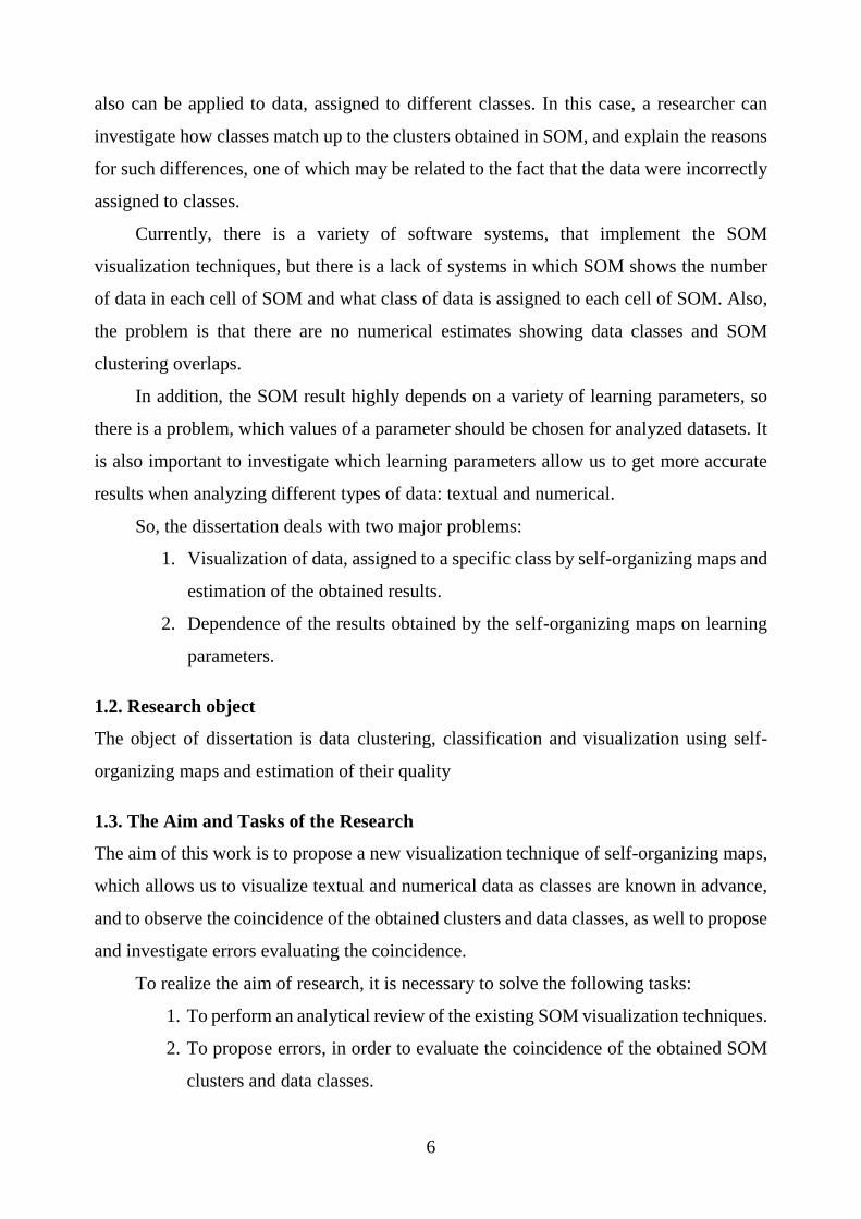
Suppose we have two SOM maps of the same size which are assigned to one of three

classes (Figure 2), in which the same data are differently visualized.

a) b)

Figure 2. Example of two SOMs: a) 𝐸1 = 0,67, 𝐸2 = 1,04, 𝐸3 = 1,63,

𝐸center = 1,32, b) 𝐸1 = 1,13, 𝐸2 = 0,71, 𝐸3 = 1, 𝐸center = 1,48

In the example of SOMs, the highlighted numbers 1, 2, 3 denote the analyzed data

class labels (𝑐 = 1, 2, 3). The pairs of numbers, in the corner of each cell indicate the cell

indices. As we can see in Figure 2a, the members of class I are located on two cells and,

in Figure 2b, the first class members are located on three cells. It is obvious that the data

are clustered more in Figure 2a. This fact is confirmed by the first error (𝐸1 = 0,67 for

SOM in Figure 2a and 𝐸1 = 1,32 for SOM in Figure 2b). The lower value of the first error

means that the class members are close to one other. The value of the first error for the

class II data of SOM in Figure 2a is larger (𝐸2 = 1,04) than that of SOM in Figure 2b

(𝐸2 = 0,71), because not only the data from the class II, but also from the class III are in

a cell. So, when we calculate the first error for the class II, we add a penalty 𝑏 =2

3.

Analogous results of the first error are obtained for the class III data. In this case, a penalty

𝑏 =1

3 is added.

The value of the error 𝐸center in both cases is similar: a) 𝐸center = 1,32,

b) 𝐸center = 1,48. However, a slightly higher value is obtained in Figure 2b, which means,

that in this case, the centers of different classes are a little bit farther from one other.

It is obvious that such an estimation of SOM is a multicriteria problem, because, at

the same time, we need to find the values of several criteria (4 criteria are estimated in

18

Figure 2). A simple solution of this problem is to use the weighted sum method, i.e. to sum

the values of errors and multiply them by the weights. However, the selection of weights

depends on the decision maker and the specificity of the problem. For example, there is a

possibility that the values of one class are more important than that of the other. In the

dissertation, such a multicriteria problem is not solved, and the values of the errors are

estimated separately.

3.3. The proposed visualization technique of SOM

The analysis of SOM systems has showed that the systems have many different

visualization techniques. However, the systems have a common disadvantage. If the

classes, which the data belong to, are known, and the labels of the classes are displayed in

the map, it is difficult to understand how many data vectors from one or other class

correspond to a cell (neuron), because usually only different (but not the same) labels are

shown. It is especially important, when the vectors from different classes fall into a SOM

cell. Also, we do not know how many data vectors are from the same class and how many

data vectors are from the different classes, and what their proportions are.

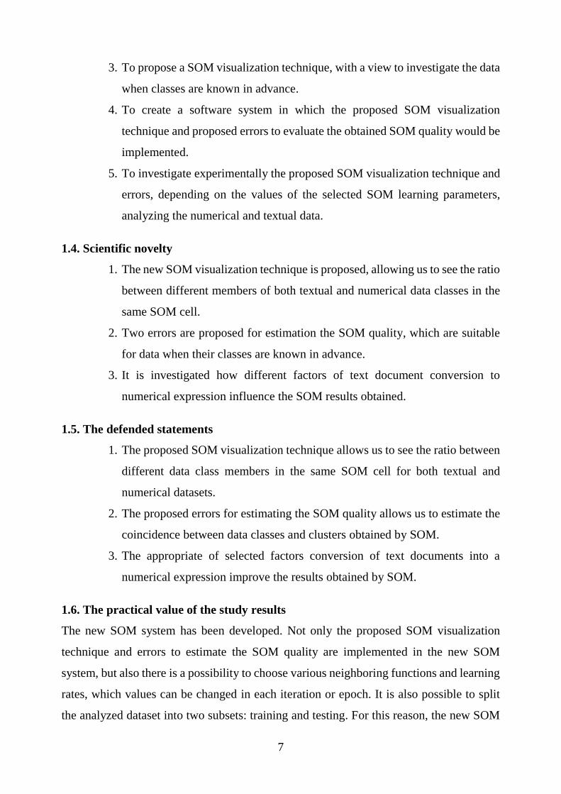
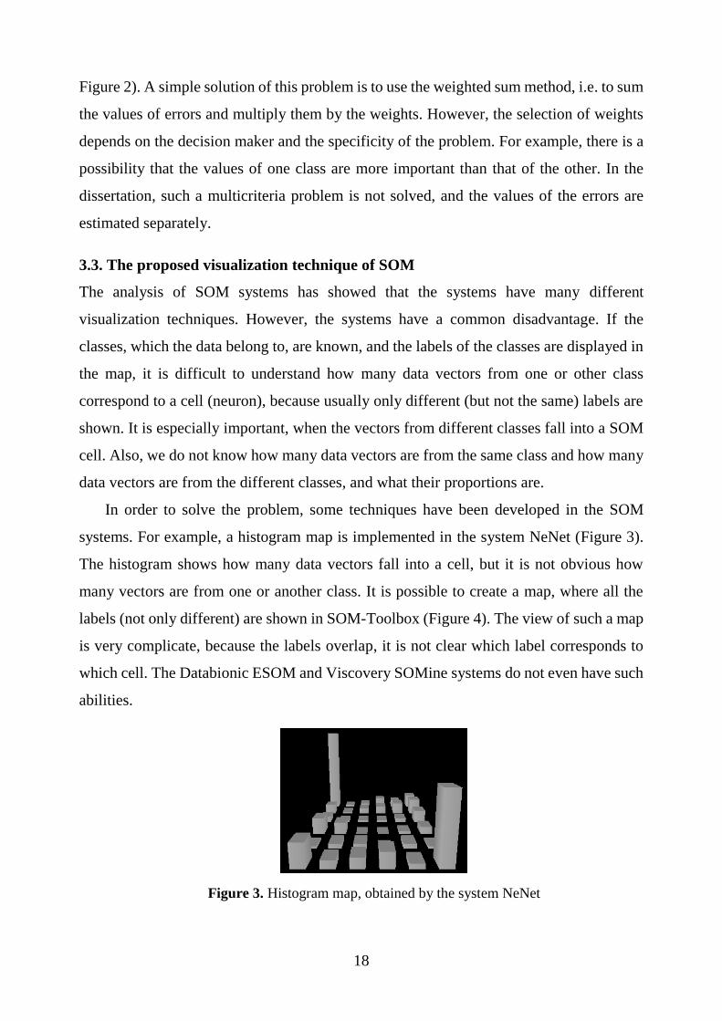
In order to solve the problem, some techniques have been developed in the SOM

systems. For example, a histogram map is implemented in the system NeNet (Figure 3).

The histogram shows how many data vectors fall into a cell, but it is not obvious how

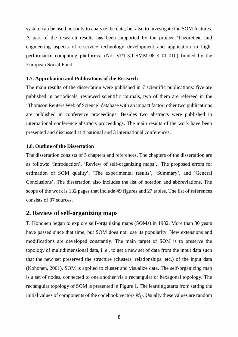
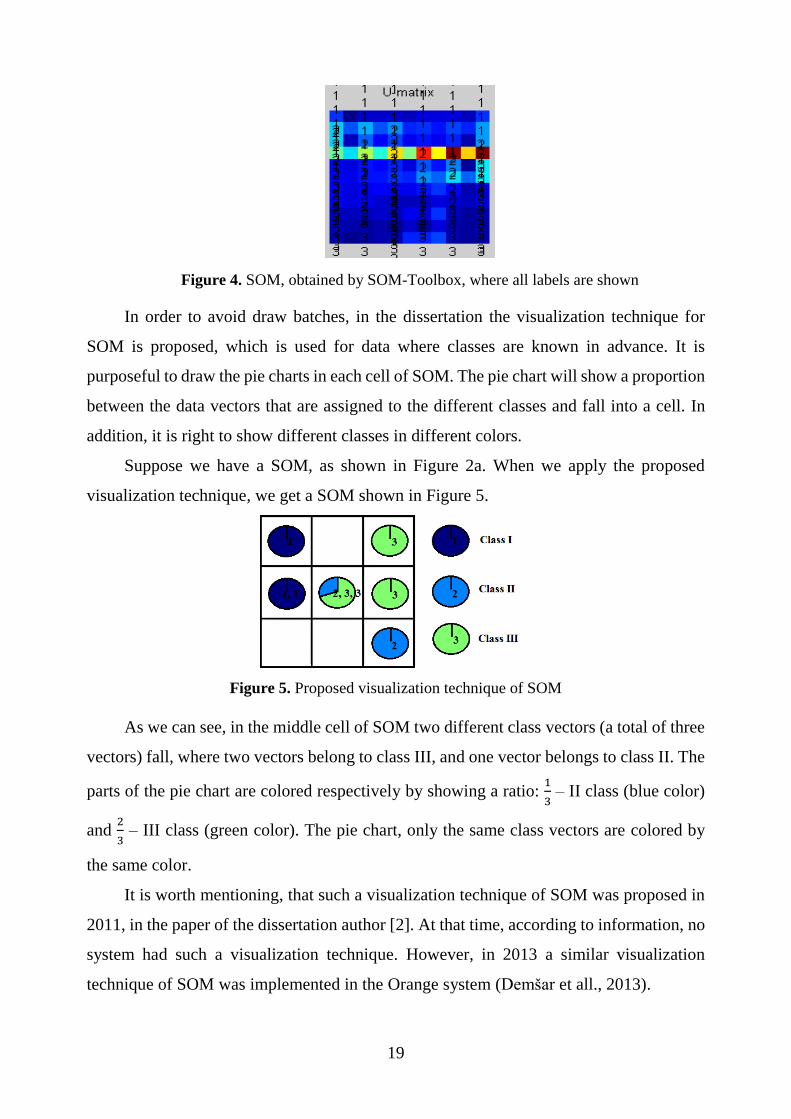
many vectors are from one or another class. It is possible to create a map, where all the

labels (not only different) are shown in SOM-Toolbox (Figure 4). The view of such a map

is very complicate, because the labels overlap, it is not clear which label corresponds to

which cell. The Databionic ESOM and Viscovery SOMine systems do not even have such

abilities.

Figure 3. Histogram map, obtained by the system NeNet

19

Figure 4. SOM, obtained by SOM-Toolbox, where all labels are shown

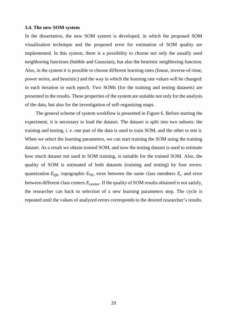
In order to avoid draw batches, in the dissertation the visualization technique for

SOM is proposed, which is used for data where classes are known in advance. It is

purposeful to draw the pie charts in each cell of SOM. The pie chart will show a proportion

between the data vectors that are assigned to the different classes and fall into a cell. In

addition, it is right to show different classes in different colors.

Suppose we have a SOM, as shown in Figure 2a. When we apply the proposed

visualization technique, we get a SOM shown in Figure 5.

Figure 5. Proposed visualization technique of SOM

As we can see, in the middle cell of SOM two different class vectors (a total of three

vectors) fall, where two vectors belong to class III, and one vector belongs to class II. The

parts of the pie chart are colored respectively by showing a ratio: 1

3 – II class (blue color)

and 2

3 – III class (green color). The pie chart, only the same class vectors are colored by

the same color.

It is worth mentioning, that such a visualization technique of SOM was proposed in

2011, in the paper of the dissertation author [2]. At that time, according to information, no

system had such a visualization technique. However, in 2013 a similar visualization

technique of SOM was implemented in the Orange system (Demšar et all., 2013).

20

3.4. The new SOM system

In the dissertation, the new SOM system is developed, in which the proposed SOM

visualization technique and the proposed error for estimation of SOM quality are

implemented. In this system, there is a possibility to choose not only the usually used

neighboring functions (bubble and Gaussian), but also the heuristic neighboring function.

Also, in the system it is possible to choose different learning rates (linear, inverse-of-time,

power series, and heuristic) and the way in which the learning rate values will be changed:

in each iteration or each epoch. Two SOMs (for the training and testing datasets) are

presented in the results. These properties of the system are suitable not only for the analysis

of the data, but also for the investigation of self-organizing maps.

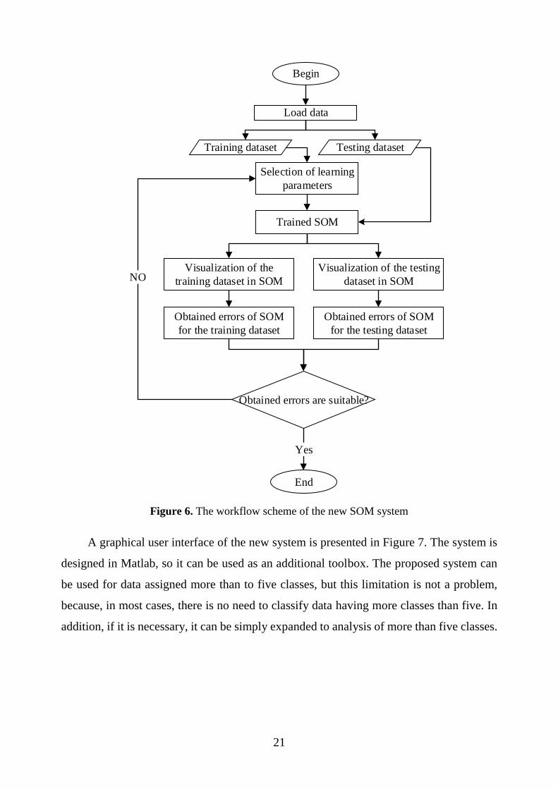
The general scheme of system workflow is presented in Figure 6. Before starting the

experiment, it is necessary to load the dataset. The dataset is split into two subsets: the

training and testing, i. e. one part of the data is used to train SOM, and the other to test it.

When we select the learning parameters, we can start training the SOM using the training

dataset. As a result we obtain trained SOM, and now the testing dataset is used to estimate

how much dataset not used in SOM training, is suitable for the trained SOM. Also, the

quality of SOM is estimated of both datasets (training and testing) by four errors:

quantization 𝐸QE, topographic 𝐸TE, error between the same class members 𝐸𝑐 and error

between different class centers 𝐸center. If the quality of SOM results obtained is not satisfy,

the researcher can back to selection of a new learning parameters step. The cycle is

repeated until the values of analyzed errors corresponds to the desired researcher’s results.

21

Begin

Load data

Training dataset Testing dataset

Selection of learning

parameters

Trained SOM

Visualization of the

training dataset in SOM

Visualization of the testing

dataset in SOM

Obtained errors of SOM

for the training dataset

Obtained errors of SOM

for the testing dataset

Obtained errors are suitable?

End

Yes

NO

Figure 6. The workflow scheme of the new SOM system

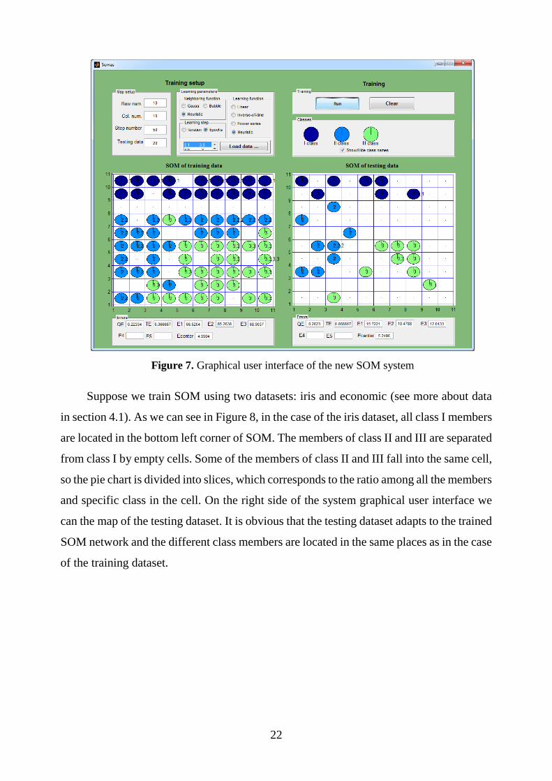
A graphical user interface of the new system is presented in Figure 7. The system is

designed in Matlab, so it can be used as an additional toolbox. The proposed system can

be used for data assigned more than to five classes, but this limitation is not a problem,

because, in most cases, there is no need to classify data having more classes than five. In

addition, if it is necessary, it can be simply expanded to analysis of more than five classes.

22

Figure 7. Graphical user interface of the new SOM system

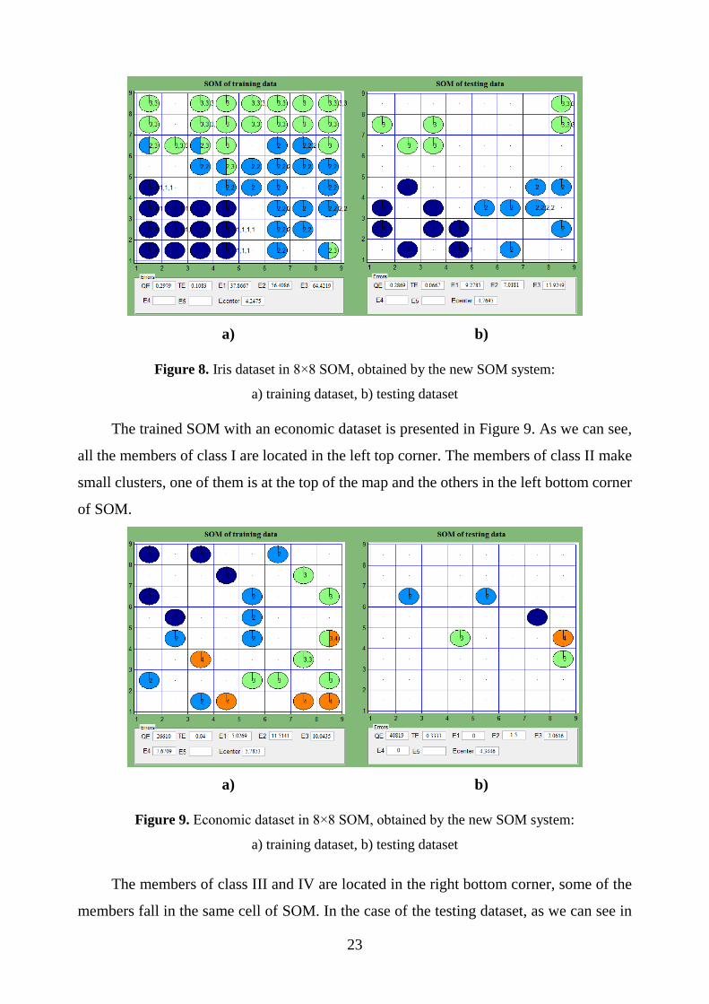
Suppose we train SOM using two datasets: iris and economic (see more about data

in section 4.1). As we can see in Figure 8, in the case of the iris dataset, all class I members

are located in the bottom left corner of SOM. The members of class II and III are separated

from class I by empty cells. Some of the members of class II and III fall into the same cell,

so the pie chart is divided into slices, which corresponds to the ratio among all the members

and specific class in the cell. On the right side of the system graphical user interface we

can the map of the testing dataset. It is obvious that the testing dataset adapts to the trained

SOM network and the different class members are located in the same places as in the case

of the training dataset.

23

a) b)

Figure 8. Iris dataset in 8×8 SOM, obtained by the new SOM system:

a) training dataset, b) testing dataset

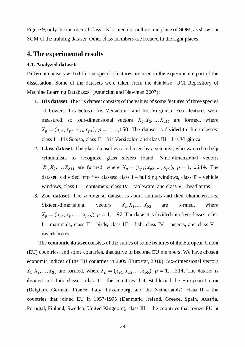
The trained SOM with an economic dataset is presented in Figure 9. As we can see,

all the members of class I are located in the left top corner. The members of class II make

small clusters, one of them is at the top of the map and the others in the left bottom corner

of SOM.

a) b)

Figure 9. Economic dataset in 8×8 SOM, obtained by the new SOM system:

a) training dataset, b) testing dataset

The members of class III and IV are located in the right bottom corner, some of the

members fall in the same cell of SOM. In the case of the testing dataset, as we can see in

24

Figure 9, only the member of class I is located not in the same place of SOM, as shown in

SOM of the training dataset. Other class members are located in the right places.

4. The experimental results

4.1. Analyzed datasets

Different datasets with different specific features are used in the experimental part of the

dissertation. Some of the datasets were taken from the database ‘UCI Repository of

Machine Learning Databases’ (Asuncion and Newman 2007):

1. Iris dataset. The iris dataset consists of the values of some features of three species

of flowers: Iris Setosa, Iris Versicolor, and Iris Virginica. Four features were

measured, so four-dimensional vectors 𝑋1, 𝑋2, … , 𝑋150 are formed, where

𝑋𝑝 = (𝑥𝑝1, 𝑥𝑝2, 𝑥𝑝3, 𝑥𝑝4), 𝑝 = 1, … ,150. The dataset is divided to three classes:

class I – Iris Setosa, class II – Iris Versicolor, and class III – Iris Virginica.

2. Glass dataset. The glass dataset was collected by a scientist, who wanted to help

criminalists to recognize glass slivers found. Nine-dimensional vectors

𝑋1, 𝑋2, … , 𝑋214 are formed, where 𝑋𝑝 = (𝑥𝑝1, 𝑥𝑝2, … , 𝑥𝑝9), 𝑝 = 1, … 214. The

dataset is divided into five classes: class I – building windows, class II – vehicle

windows, class III – containers, class IV – tableware, and class V – headlamps.

3. Zoo dataset. The zoological dataset is about animals and their characteristics.

Sixteen-dimensional vectors 𝑋1, 𝑋2, … , 𝑋92 are formed, where

𝑋𝑝 = (𝑥𝑝1, 𝑥𝑝2, … , 𝑥𝑝16), 𝑝 = 1, … 92. The dataset is divided into five classes: class

I – mammals, class II – birds, class III – fish, class IV – insects, and class V –

invertebrates.

The economic dataset consists of the values of some features of the European Union

(EU) countries, and some countries, that strive to become EU members. We have chosen

economic indices of the EU countries in 2009 (Eurostat, 2010). Six-dimensional vectors

𝑋1, 𝑋2, … , 𝑋31 are formed, where 𝑋𝑝 = (𝑥𝑝1, 𝑥𝑝2, … , 𝑥𝑝6), 𝑝 = 1, … 214. The dataset is

divided into four classes: class I – the countries that established the European Union

(Belgium, German, France, Italy, Luxemburg, and the Netherlands), class II – the

countries that joined EU in 1957-1995 (Denmark, Ireland, Greece, Spain, Austria,

Portugal, Finland, Sweden, United Kingdom), class III – the countries that joined EU in

25

2004-2007 (Czech Republic, Estonia, Cyprus, Latvia, Lithuania, Hungary, Malta, Poland,

Slovenia, Slovakia, Bulgaria, Romania), and class IV – the countries that are seeking to

be EU members (Macedonia, Turkey, Iceland, Croatia).

The dataset of different text documents was also used in the experimental

investigation. The dimension of vectors is different, because it depends on the length of

the text document dictionary.

1. Orders of the Ministries. The document of eight text areas taken from the

document database of Seimas of the Republic of Lithuania (LRS, 2013) have been

analyzed in the experimental investigation. 15 similar size orders were selected

randomly from Ministries of Finance, Culture, Transport and Communication,

Health, Education and Science, Economy, the Interior and Agriculture. Using

these orders, three dataset have been created: 𝑋1 = {𝑋11, 𝑋2

1, … , 𝑋601 }, 𝑋2 = {𝑋1

2,

𝑋22, … , 𝑋60

2 }, and 𝑋3 = {𝑋13, 𝑋2

3, … , 𝑋603 }. All the datasets were divided into four

classes.

The first dataset represents: class I – Health, class II – Education and

Science, class III – the Interior, and class IV – Agriculture ministries. The second

dataset represents: class I – Finance, class II – Culture, class III – Transport and

Communication, and IV class – Agriculture ministries. The third dataset

represents: class I – Finance, class II – Economy, class III – the Interior, and class

IV – Agriculture ministries.

2. Scientific papers I. 60 scientific papers𝑋1, 𝑋2, … , 𝑋60 have been taken randomly

from the Internet freely accessible databases (SpringerLink, ScienceDirect, etc.).

The dataset is divided into four classes: class I – papers about artificial neural

networks (ANN), class II – papers about bioinformatics, class III – papers about

optimization, and class IV – papers about self-organizing maps.

3. Scientific papers II. 45 scientific papers 𝑋1, 𝑋2, … , 𝑋60 have been taken randomly

from the Internet freely accessible databases (SpringerLink, ScienceDirect, etc.).

The dataset is divided into three classes: class I – papers about Pareto

optimization, class II – papers about simplex optimization, and class III – papers

about genetic optimization.

26

Such a dataset distribution and class assignment has been performed by the author

of the dissertation.

4.1. Comparative analysis of SOM systems

The proposed SOM system in subsection 3.4 has been compared with other SOM systems

reviewed in subsection 2.5: NeNet, SOM-Toolbox, Databionic ESOM, Viscovery

SOMine, and Orange. After a comparative analysis has been made, we can see advantages

and disadvantages of various systems (Table 3). The systems are compared according to

the following:

K1. There is a possibility to analyze data sets of different sizes.

K2. It is easy to prepare data to the system, there is a possibility to prepare data in

the form of a simple text file.

K3. There is a possibility to split the data into training and testing datasets.

K4. It is possible to use more than two learning parameters.

K5. There is a possibility to use more than one neighboring function.

K6. There is a possibility to change learning rate values in each epoch or each

iteration.

K7. There is a possibility to visualize all data vectors labels in the same cell of SOM.

K8. There is a possibility to see the ratio among different data vectors in the same

cell of SOM.

K9. The distance between neurons are displayed in the SOM.

K10. There is a possibility to choose different SOM visualization techniques.

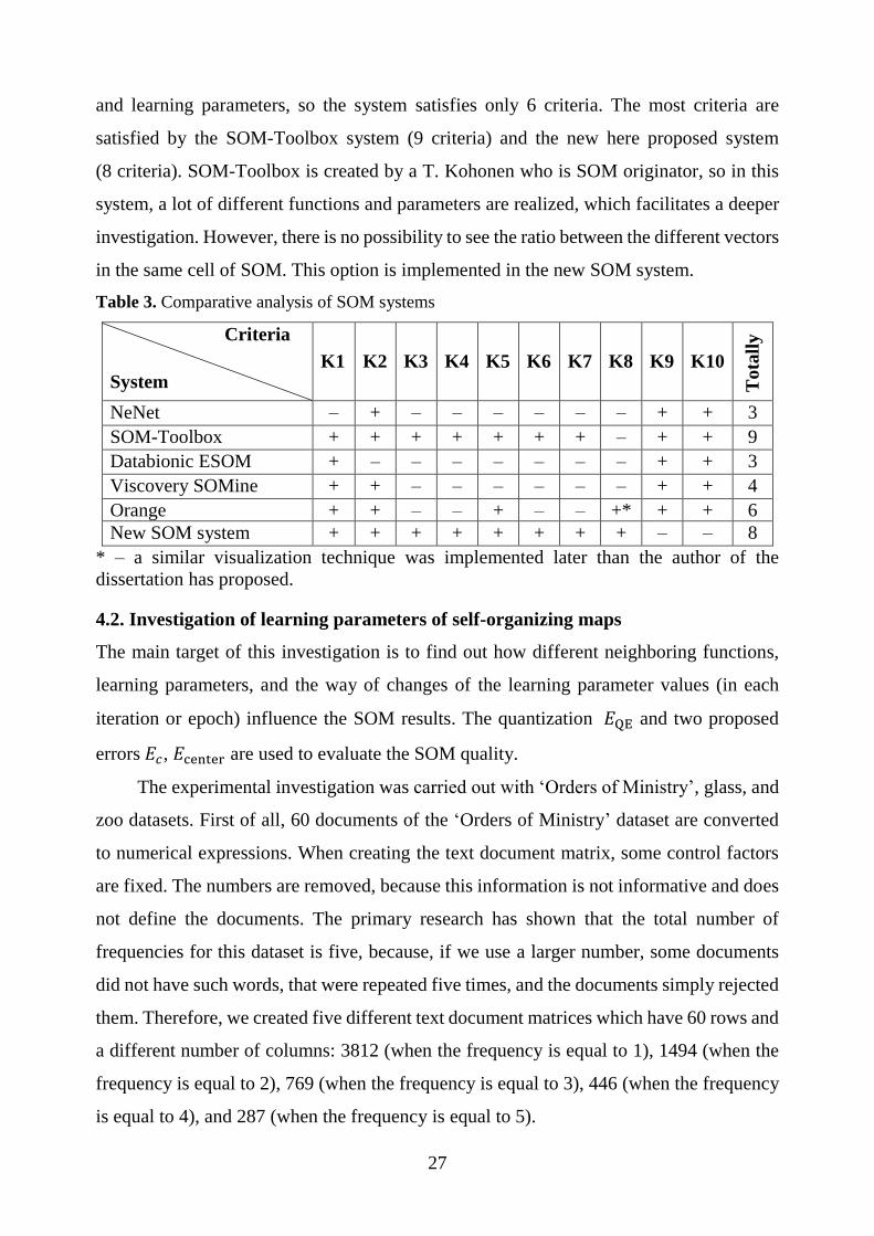
In Table 3, we can see which criteria are satisfied by all the analyzed systems. The last

column indicates the number of criteria satisfied by the system. The sign ‘+’ means that

the system satisfies the criteria and the sign ‘-‘ means that criteria are not satisfied. As we

can see, the systems NeNet and Databionic satisfy the least number of criteria (3 criteria).

These two systems have only the basic functions and control parameters, so if we want to

carry out a more detailed investigation we have to deal with one or other restriction. The

Viscovery SOMine system (4 criteria) has various visualization techniques, but we can

also select only the basic learning parameters. A similar visualization technique, proposed

in the dissertation was implemented in Orange system, but there are no other important

parameters that could help for deeper investigation, such as various neighboring functions

27

and learning parameters, so the system satisfies only 6 criteria. The most criteria are

satisfied by the SOM-Toolbox system (9 criteria) and the new here proposed system

(8 criteria). SOM-Toolbox is created by a T. Kohonen who is SOM originator, so in this

system, a lot of different functions and parameters are realized, which facilitates a deeper

investigation. However, there is no possibility to see the ratio between the different vectors

in the same cell of SOM. This option is implemented in the new SOM system.

Table 3. Comparative analysis of SOM systems

Criteria

System K1 K2 K3 K4 K5 K6 K7 K8 K9 K10

Tota

lly

NeNet – + – – – – – – + + 3

SOM-Toolbox + + + + + + + – + + 9

Databionic ESOM + – – – – – – – + + 3

Viscovery SOMine + + – – – – – – + + 4

Orange + + – – + – – +* + + 6

New SOM system + + + + + + + + – – 8

* – a similar visualization technique was implemented later than the author of the

dissertation has proposed.

4.2. Investigation of learning parameters of self-organizing maps

The main target of this investigation is to find out how different neighboring functions,

learning parameters, and the way of changes of the learning parameter values (in each

iteration or epoch) influence the SOM results. The quantization 𝐸QE and two proposed

errors 𝐸𝑐, 𝐸center are used to evaluate the SOM quality.

The experimental investigation was carried out with ‘Orders of Ministry’, glass, and

zoo datasets. First of all, 60 documents of the ‘Orders of Ministry’ dataset are converted

to numerical expressions. When creating the text document matrix, some control factors

are fixed. The numbers are removed, because this information is not informative and does

not define the documents. The primary research has shown that the total number of

frequencies for this dataset is five, because, if we use a larger number, some documents

did not have such words, that were repeated five times, and the documents simply rejected

them. Therefore, we created five different text document matrices which have 60 rows and

a different number of columns: 3812 (when the frequency is equal to 1), 1494 (when the

frequency is equal to 2), 769 (when the frequency is equal to 3), 446 (when the frequency

is equal to 4), and 287 (when the frequency is equal to 5).

28

The primary research has shown that the size of the map and a larger epoch or

iteration number do not affect the results essentially. Therefore in all the experiments the

map size is 10×10 and the epoch numbers are equal to 50. The number of epochs multiplied

by the number of data items N corresponds to the number of iterations. Each experiment

is repeated 10 times with different initial values of neurons 𝑀𝑖𝑗. The averages of the

quantization error and all the other errors are calculated. The self-organizing map is trained

using 80% of the whole dataset, and the rest 20% of the dataset are used for testing in order

to see how well the testing dataset adapts to the trained SOM.

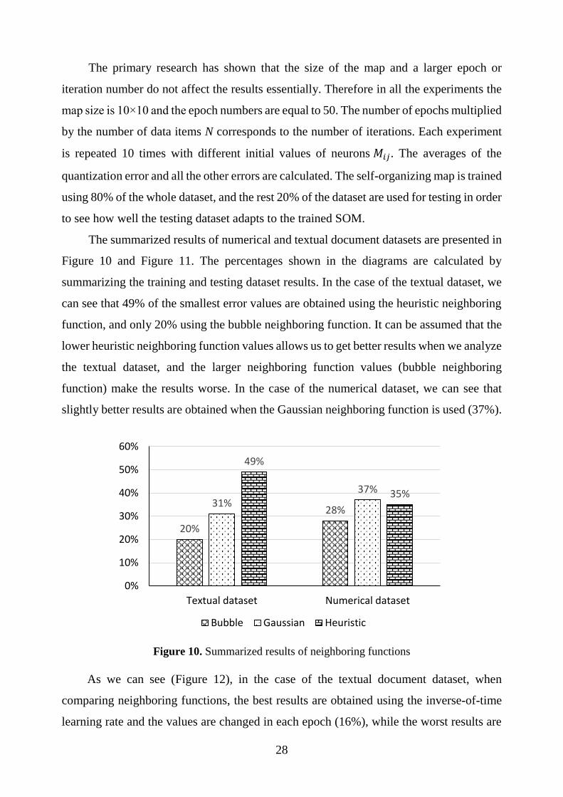
The summarized results of numerical and textual document datasets are presented in

Figure 10 and Figure 11. The percentages shown in the diagrams are calculated by

summarizing the training and testing dataset results. In the case of the textual dataset, we

can see that 49% of the smallest error values are obtained using the heuristic neighboring

function, and only 20% using the bubble neighboring function. It can be assumed that the

lower heuristic neighboring function values allows us to get better results when we analyze

the textual dataset, and the larger neighboring function values (bubble neighboring

function) make the results worse. In the case of the numerical dataset, we can see that

slightly better results are obtained when the Gaussian neighboring function is used (37%).

Figure 10. Summarized results of neighboring functions

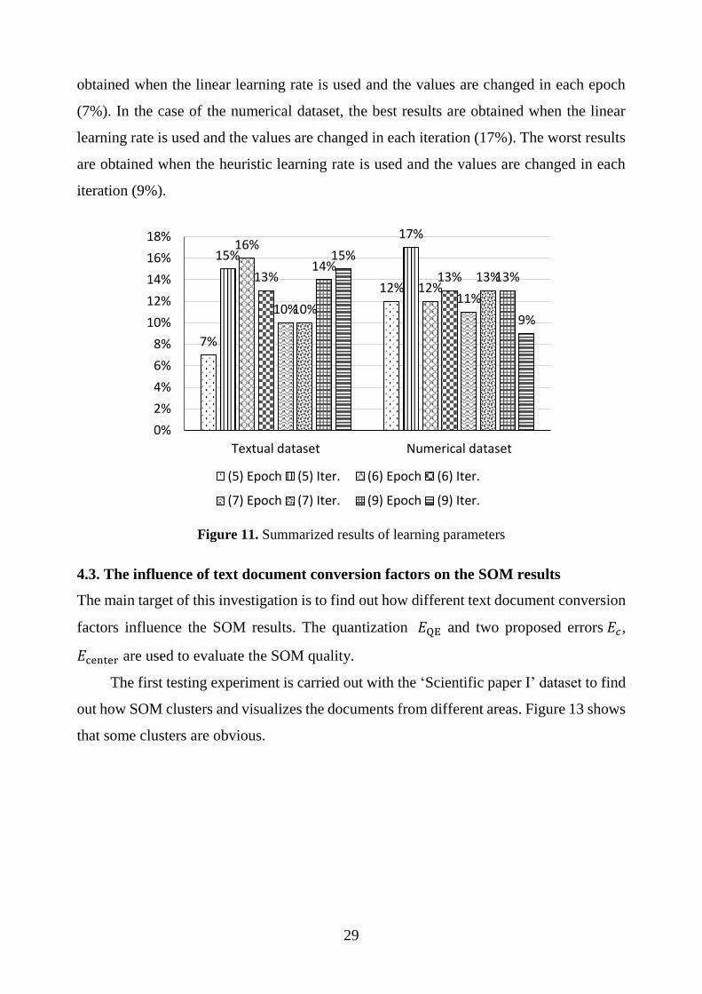
As we can see (Figure 12), in the case of the textual document dataset, when

comparing neighboring functions, the best results are obtained using the inverse-of-time

learning rate and the values are changed in each epoch (16%), while the worst results are

20%

28%31%

37%

49%

35%

0%

10%

20%

30%

40%

50%

60%

Textual dataset Numerical dataset

Bubble Gaussian Heuristic

29

obtained when the linear learning rate is used and the values are changed in each epoch

(7%). In the case of the numerical dataset, the best results are obtained when the linear

learning rate is used and the values are changed in each iteration (17%). The worst results

are obtained when the heuristic learning rate is used and the values are changed in each

iteration (9%).

Figure 11. Summarized results of learning parameters

4.3. The influence of text document conversion factors on the SOM results

The main target of this investigation is to find out how different text document conversion

factors influence the SOM results. The quantization 𝐸QE and two proposed errors 𝐸𝑐,

𝐸center are used to evaluate the SOM quality.

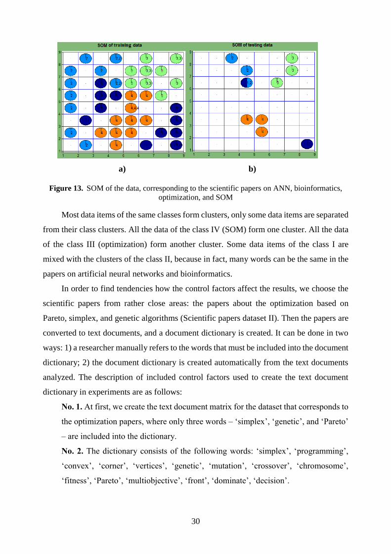
The first testing experiment is carried out with the ‘Scientific paper I’ dataset to find

out how SOM clusters and visualizes the documents from different areas. Figure 13 shows

that some clusters are obvious.

7%

12%

15%

17%16%

12%13% 13%

10%11%

10%

13%14%

13%

15%

9%

0%

2%

4%

6%

8%

10%

12%

14%

16%

18%

Textual dataset Numerical dataset

(5) Epoch (5) Iter. (6) Epoch (6) Iter.

(7) Epoch (7) Iter. (9) Epoch (9) Iter.

30

a) b)

Figure 13. SOM of the data, corresponding to the scientific papers on ANN, bioinformatics,

optimization, and SOM

Most data items of the same classes form clusters, only some data items are separated

from their class clusters. All the data of the class IV (SOM) form one cluster. All the data

of the class III (optimization) form another cluster. Some data items of the class I are

mixed with the clusters of the class II, because in fact, many words can be the same in the

papers on artificial neural networks and bioinformatics.

In order to find tendencies how the control factors affect the results, we choose the

scientific papers from rather close areas: the papers about the optimization based on

Pareto, simplex, and genetic algorithms (Scientific papers dataset II). Then the papers are

converted to text documents, and a document dictionary is created. It can be done in two

ways: 1) a researcher manually refers to the words that must be included into the document

dictionary; 2) the document dictionary is created automatically from the text documents

analyzed. The description of included control factors used to create the text document

dictionary in experiments are as follows:

No. 1. At first, we create the text document matrix for the dataset that corresponds to

the optimization papers, where only three words – ‘simplex’, ‘genetic’, and ‘Pareto’

– are included into the dictionary.

No. 2. The dictionary consists of the following words: ‘simplex’, ‘programming’,

‘convex’, ‘corner’, ‘vertices’, ‘genetic’, ‘mutation’, ‘crossover’, ‘chromosome’,

‘fitness’, ‘Pareto’, ‘multiobjective’, ‘front’, ‘dominate’, ‘decision’.

31

No. 3. The experiment is carried out disregarding the common word list as a

document dictionary is being created.

No. 4. The common word list created by the Text to Matrix Generator toolbox

(TMG), is used. This common word list has more than 300 words, such as ‘there’,

‘where’, ‘here’, ‘some’, etc.

No. 5. The TMG toolbox has a common word list unsuitable for scientific papers.

So, considering that the papers about optimization are analyzed here, we create a new

common word list including the words such as ‘function’, ‘fig’, ‘table’, ‘formula’,

‘optimization’, ‘present’, ‘minimum’, ‘maximum’, ‘function’, ‘variable’, etc.

No. 6-8. The experiments analogous to No. 3-5, only the stemming algorithm used

in addition.

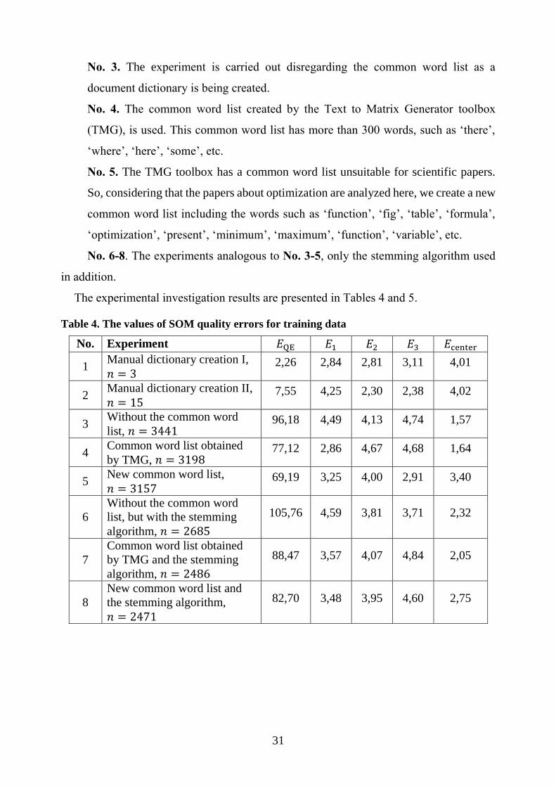
The experimental investigation results are presented in Tables 4 and 5.

Table 4. The values of SOM quality errors for training data

No. Experiment 𝐸QE 𝐸1 𝐸2 𝐸3 𝐸center

1 Manual dictionary creation I,

𝑛 = 3 2,26 2,84 2,81 3,11 4,01

2 Manual dictionary creation II,

𝑛 = 15 7,55 4,25 2,30 2,38 4,02

3 Without the common word

list, 𝑛 = 3441 96,18 4,49 4,13 4,74 1,57

4 Common word list obtained

by TMG, 𝑛 = 3198 77,12 2,86 4,67 4,68 1,64

5 New common word list,

𝑛 = 3157 69,19 3,25 4,00 2,91 3,40

6

Without the common word

list, but with the stemming

algorithm, 𝑛 = 2685

105,76 4,59 3,81 3,71 2,32

7

Common word list obtained

by TMG and the stemming

algorithm, 𝑛 = 2486

88,47 3,57 4,07 4,84 2,05

8

New common word list and

the stemming algorithm,

𝑛 = 2471

82,70 3,48 3,95 4,60 2,75

32

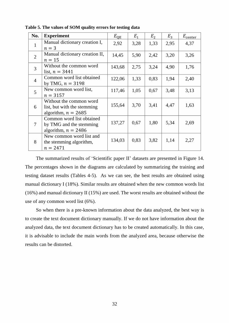
Table 5. The values of SOM quality errors for testing data

No. Experiment 𝐸QE 𝐸1 𝐸2 𝐸3 𝐸center

1 Manual dictionary creation I,

𝑛 = 3 2,92 3,28 1,33 2,95 4,37

2 Manual dictionary creation II,

𝑛 = 15 14,45 5,90 2,42 3,20 3,26

3 Without the common word

list, 𝑛 = 3441 143,68 2,75 3,24 4,90 1,76

4 Common word list obtained

by TMG, 𝑛 = 3198 122,06 1,33 0,83 1,94 2,40

5 New common word list,

𝑛 = 3157 117,46 1,05 0,67 3,48 3,13

6

Without the common word

list, but with the stemming

algorithm, 𝑛 = 2685

155,64 3,70 3,41 4,47 1,63

7

Common word list obtained

by TMG and the stemming

algorithm, 𝑛 = 2486

137,27 0,67 1,80 5,34 2,69

8

New common word list and

the stemming algorithm,

𝑛 = 2471

134,03 0,83 3,82 1,14 2,27

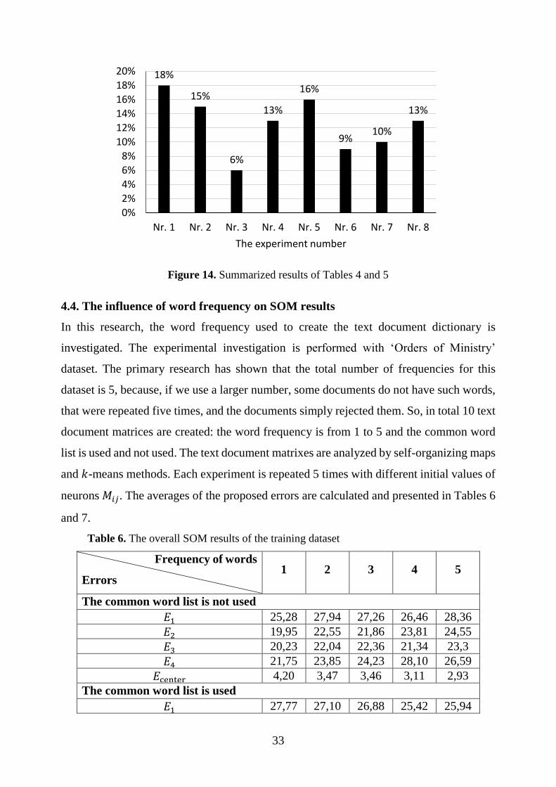
The summarized results of ‘Scientific paper II’ datasets are presented in Figure 14.

The percentages shown in the diagrams are calculated by summarizing the training and

testing dataset results (Tables 4-5). As we can see, the best results are obtained using

manual dictionary I (18%). Similar results are obtained when the new common words list

(16%) and manual dictionary II (15%) are used. The worst results are obtained without the

use of any common word list (6%).

So when there is a pre-known information about the data analyzed, the best way is

to create the text document dictionary manually. If we do not have information about the

analyzed data, the text document dictionary has to be created automatically. In this case,

it is advisable to include the main words from the analyzed area, because otherwise the

results can be distorted.

33

Figure 14. Summarized results of Tables 4 and 5

4.4. The influence of word frequency on SOM results

In this research, the word frequency used to create the text document dictionary is

investigated. The experimental investigation is performed with ‘Orders of Ministry’

dataset. The primary research has shown that the total number of frequencies for this

dataset is 5, because, if we use a larger number, some documents do not have such words,

that were repeated five times, and the documents simply rejected them. So, in total 10 text

document matrices are created: the word frequency is from 1 to 5 and the common word

list is used and not used. The text document matrixes are analyzed by self-organizing maps

and 𝑘-means methods. Each experiment is repeated 5 times with different initial values of

neurons 𝑀𝑖𝑗. The averages of the proposed errors are calculated and presented in Tables 6

and 7.

Table 6. The overall SOM results of the training dataset

Frequency of words

Errors 1 2 3 4 5

The common word list is not used

𝐸1 25,28 27,94 27,26 26,46 28,36

𝐸2 19,95 22,55 21,86 23,81 24,55

𝐸3 20,23 22,04 22,36 21,34 23,3

𝐸4 21,75 23,85 24,23 28,10 26,59

𝐸center 4,20 3,47 3,46 3,11 2,93

The common word list is used

𝐸1 27,77 27,10 26,88 25,42 25,94

18%

15%

6%

13%

16%

9%10%

13%

0%

2%

4%

6%

8%

10%

12%

14%

16%

18%

20%

Nr. 1 Nr. 2 Nr. 3 Nr. 4 Nr. 5 Nr. 6 Nr. 7 Nr. 8

The experiment number

34

𝐸2 20,13 22,85 21,40 23,31 23,29

𝐸3 17,43 19,39 20,77 23,1 26,26

𝐸4 23,11 23,87 25,58 24,69 26,78

𝐸center 4,10 3,79 3,34 3,54 3,10

Table 7. The overall SOM results of the testing dataset

Frequency of words

Errors 1 2 3 4 5

The common word list is not used

𝐸1 2,04 3,56 3,47 3,52 4,60

𝐸2 1,93 2,96 2,59 2,66 3,34

𝐸3 3,33 3,45 4,27 3,32 5,12

𝐸4 1,68 2,92 2,46 3,31 2,18

𝐸center 4,67 4,45 3,78 3,41 3,37

The common word list is used

𝐸1 2,99 2,98 2,76 3,71 3,86

𝐸2 2,38 2,53 2,59 3,17 2,92

𝐸3 3,06 3,16 3,43 3,99 6,28

𝐸4 2,56 2,51 3,26 2,14 2,22

𝐸center 4,59 4,54 3,76 3,88 3,07

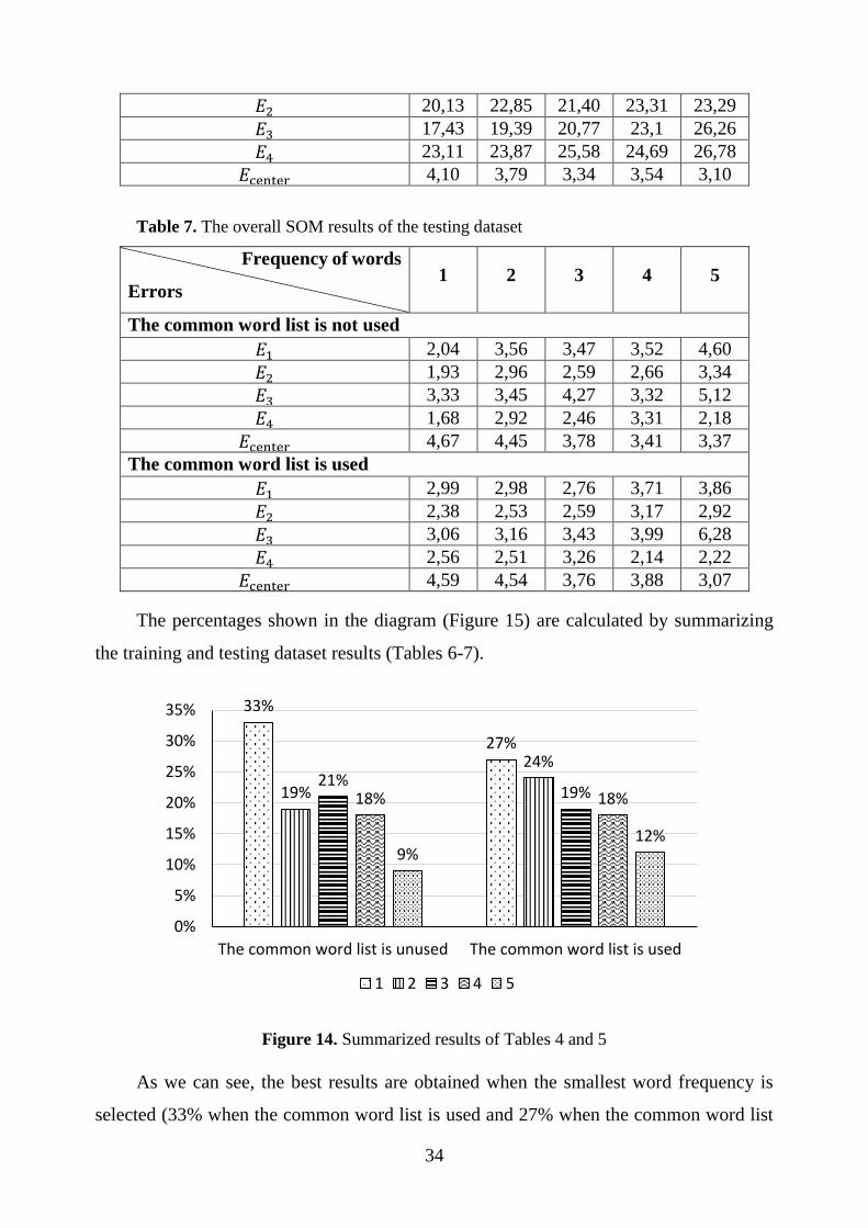
The percentages shown in the diagram (Figure 15) are calculated by summarizing

the training and testing dataset results (Tables 6-7).

Figure 14. Summarized results of Tables 4 and 5

As we can see, the best results are obtained when the smallest word frequency is

selected (33% when the common word list is used and 27% when the common word list

33%

27%

19%

24%21%

19%18% 18%

9%12%

0%

5%

10%

15%

20%

25%

30%

35%

The common word list is unused The common word list is used

1 2 3 4 5

35

is not used). When the word frequency is increased, the values of the proposed errors

𝐸1, 𝐸2, 𝐸3, 𝐸4, 𝐸center become worse. The worst results are obtained when the common

word list is not used and the word frequency is equal to 5, i. e. all the words are included

in the text document dictionary (9% of all cases).

It is useful to compare the SOM results to that obtained by one of the most popular

clustering method 𝑘-means (MacQueen, 1967). At first, the number 𝐾 of desired clusters

is selected and initial values of cluster centers are assigned. Then, each data item is

assigned to the cluster with the closest centers, and new centers for each cluster are

computed. The steps are repeated iteratively until the stop or convergence criterion is

satisfied. The convergence criterion can be based on the squared error (averaged difference

between the cluster centers and the items assigned to the clusters). The stop criterion can

be a high number of iteration steps. Usually the 𝑘-means method quality is estimated by

calculating the square error between the center of the cluster and the cluster assigned to

the data:

𝐸𝐴𝐾𝑆 = ∑ ∑ ‖𝑋𝑗𝑖 − 𝐶𝑖‖

2𝜇𝑗=1

𝐾𝑖=1 .

In the experimental investigation the data are assigned to the classes, so it is

important to evaluate whether obtained clusters match the vector classes. First of all, the

data are clustered into clusters the number of which corresponds to the class number of

the data. Later, the overlaps of the classes and obtained clusters are determined, i. e. the

vectors of some dataset class have to be assigned to the cluster which has the largest

number of members of that class. Then the number of vectors wrongly assigned to the

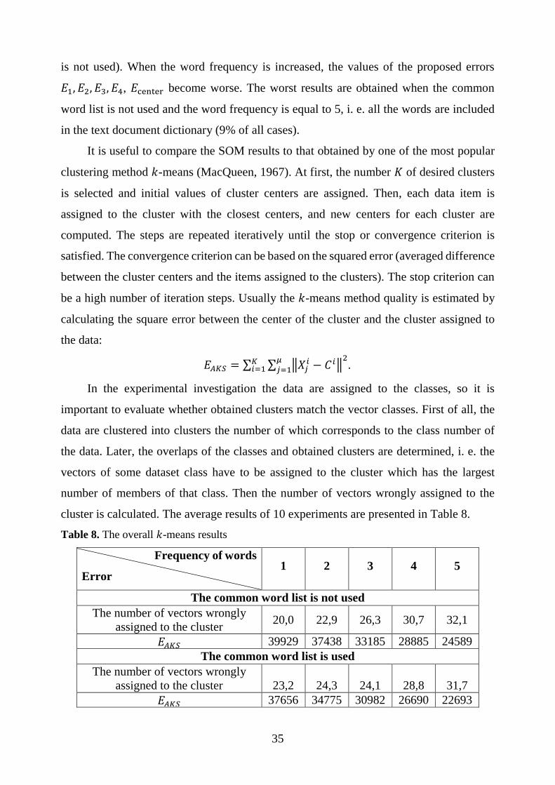
cluster is calculated. The average results of 10 experiments are presented in Table 8.

Table 8. The overall 𝑘-means results

Frequency of words

Error 1 2 3 4 5

The common word list is not used

The number of vectors wrongly

assigned to the cluster 20,0 22,9 26,3 30,7 32,1

𝐸𝐴𝐾𝑆 39929 37438 33185 28885 24589

The common word list is used

The number of vectors wrongly

assigned to the cluster 23,2 24,3 24,1 28,8 31,7

𝐸𝐴𝐾𝑆 37656 34775 30982 26690 22693

36

Each time when the word frequency is increased, the number of vector wrongly

assigned to the cluster results are the larger, except only the case, where the word

frequency is equal to 2 and the common word list is used. In all cases, where the frequency

of the words is decreasing, the values of error 𝐸𝐴𝐾𝑆 are decreasing too. However,

evaluation of the results, obtained by error 𝐸𝐴𝐾𝑆, is not appropriate, since the size of a

dataset is various, and the lower value of 𝐸𝐴𝐾𝑆 does not show the clustering accuracy. In

most cases, the accurate results are obtained where the minimal frequency of the word is

selected, and the worst results are where the frequency of the word is equal to 5.

5. Summary and General Conclusions

The investigation of self-organizing maps yield the following results: the new SOM

visualization technique is proposed; new errors for estimation of SOM quality are

proposed, which allows us to compare the coincidence between classes and clusters of

several SOMs; the new SOM system is created in which the proposed visualization

technique, errors and various learning parameters are implemented; the influence of

different SOM learning parameters and text document conversion to numerical expression

factors on the obtained SOM results has been investigated.

The experimental investigation has shown that the proposed visualization technique

and proposed errors are useful for dataset analysis, when data classes are known in

advance. The experimental results led to the following conclusions:

1. The proposed errors properly estimate the coincidence of the data classes and

clusters obtained in SOM.

2. The proposed visualization technique allows us to visualize the ratio between

different class members which fall in the same cell of SOM.

3. In the case of the textual document dataset, more accurate results are obtained

according to the proposed errors when heuristic neighboring function is used

(49% of all cases), the Gaussian neighboring function – 31%, and bubble –

20% of all cases; in the case of the numerical dataset, better SOM results are

obtained when the Gaussian neighboring function is used (37% of all cases),

but they do not differ very much from the results obtained using the heuristic

neighboring function (35% of all cases).

37

4. Depending on the learning rate selection, the best SOM results for the textual

document dataset (in the case of proposed errors) are obtained, when the

inverse-of-time learning rate is used and the values are changed in each epoch

(16% of all cases). The worst results are obtained when the linear learning

rate is used and the values are changed in each epoch (7% of all cases). In the

case of the numerical dataset, the best results are obtained when the linear

learning rate is used and the values are changed in each iteration (17% of all

cases), and the worse results when heuristic learning rate is used and the

values are changed in each iteration (9% of all cases).

5. Investigations of the text document, used when the text document dataset is

converted into the numerical expression show that more accurate results (in

the case of proposed errors) are obtained, if the text document dictionary is

created manually (18% and 15% of all cases), i. e. the researcher by himself

includes the words to the text document dictionary. When the automatic text

document dictionary creation is used, the accurate results are obtained when

the new common word list is used (16% of all cases) to create the text

document dictionary and the stemming algorithm is not used.

6. The investigation of the word frequency influence on the SOM results shows

that by increasing the minimum number of word frequencies, the overall

accuracy of the SOM results declines; the most accurate results are obtained

when the minimum number of word frequencies is equal to 1 (approximately

30%), and the worst results are when the number of word frequencies is equal

to 5 (approximately 10,5%).

List of Literature Referenced in this Summary 1. Asuncion, A., Newman, D. J. (2007). UCI Machine Learning Repository, Irvine,

CA: University of California, School of Information and Computer.

http://www.ics.uci.edu/~mlearn/MLRepository.html

2. Demšar, J., Curk, T., & Erjavec, A. (2013). Orange: Data Mining Toolbox in

Python; Journal of Machine Learning Research 14(Aug): 2349–2353.

3. Dzemyda, G. (2001). Visualization of a Set of Parameters Characterized by their

Correlation Matrix. Computational Statistics and Data Analysis, 36(1): 15–30.

38

4. Eurostat (2010): http://epp.eurostat.ec.europa.eu/portal/page/portal/eurostat/home.

5. Iwasaki, Y., Abe, T.,Wada, Y.,Wada, K., Ikemura, T. (2013). Novel Bioinformatics

Strategies for Prediction of Directional Sequence Changes in Influenza Virus

Genomes and for Surveillance of Potentially Hazardous Strains. BMC Infectious

Diseases 13(386).

6. Kaski, S., Honkela, T., Lagus, K., and Kohonen, T. (1998). WEBSOM – Self-

Organizing Maps of Document Collections. Neurocomputing 21:101–117.

7. Kohonen, T. (2001). Self-Organizing Maps, 3rd ed., Springer Series in Information

Sciences. Berlin: Springer-Verlag.

8. Lietuvos Respublikos Seimas (2013): http://www3.lrs.lt/dokpaieska/forma_l.htm

9. MacQueen, J. (1967). Some methods for classification and analysis of multivariate

observations, In Le Cam, L. M., and Neyman, J., editors. In Proccedings of the

Proceedings of the Fifth Berkeley Symposium on Mathematical Statistics and

Probability, Statistics. I, 281–297. Berkeley and Los Angeles: University of

California Press.

10. Manning, D. C, Raghavan, P. and Schütze, H. (2008). Introduction to Information

Retrieval, Cambridge University Press.

11. Porter, M. F. (1980). An Algorithm for Suffix Stripping. Program, 14: 130–137.

12. Prakash, A. (2013). Reconstructing Self Organizing Maps as Spider Graphs for

Better Visual Interpretation of Large Unstructured Datasets. Infosys Lab Briefings

11 (1).

13. Strickert, M., Hammer, B. (2005). Merge SOM for temporal data. Neurocomputing

64: 39–72.

14. Voegtlin, T. (2002). Recursive Self-Organizing Maps. Neural Networks 15 (8-9),

979–992.

15. Zeimpekis, D., Gallopoulos, E. (2005). TMG: A Matlab Toolbox for Generating

Term-Document Matrices from Text Collections, Technical Report HPCLAB-SCG

1/01-05, University of Patras, GR-26500, Patras, Greece.

39

List of Publications on Topic of Dissertation

The articles published in the peer-reviewed periodical publications:

1. Stefanovič P., Kurasova O. (2009). Saviorganizuojančių neuroninių tinklų sistemų

lyginamoji analizė. Informacijos mokslai. ISSN 1392-0561. T. 50, pp. 334–339.

2. Stefanovič, P., Kurasova, O. (2011). Visual analysis of self-organizing maps.

Nonlinear Analysis: Modelling and Control. Vol. 16, no. 4. ISSN 1392-5113

pp. 488–504 (Impact Factor 2013: 0,914).

3. Stefanovič, P., Kurasova, O. (2013). Tekstinių dokumentų panašumų paieška

naudojant saviorganizuojančius neuroninius tinklus ir 𝑘-vidurkių metodą.

Informacijos mokslai. T. 65, ISSN 1392-0561 pp. 24–33.

4. Stefanovič, P., Kurasova, O. (2014). Creation of text document matrices and

visualization by SOM. Information Technology and Control. Vol. 43, no. 1. ISSN

1392-124X pp. 37–46 (Impact Factor 2013: 0,813).

5. Stefanovič, P., Kurasova, O. (2014). Investigation on learning parameters of self-

organizing maps. Baltic Journal of Modern Computing. Vol. 2, no. 2. ISSN 2255-

8942 pp. 45–55.

The articles published in the conference proceedings:

1. Stefanovič, P., Kurasova, O. (2011). Influence of Learning Rates and Neighboring

Functions on Self-Organizing Maps. In: J. Laaksonen, T. Honkela (Eds.). Advances

in Self-Organizing Maps: 8th International Workshop, WSOM 2011, Espoo,

Finland, June 13–15, 2011: Proceedings. Book Series: Lecture Notes in Computer

Science. Vol. 6731. ISBN 9783642215 pp. 141–150.

2. Kurasova, O., Marcinkevičius, V., Medvedev, V., Rapečka, A., and Stefanovič, P.

(2014). Strategies for Big Data Clustering. Proceedings of 26th IEEE International

Conference on Tools with Artificial Intelligence, ISSN 1082-3409 pp. 740–747.

The abstracts published in conference abstracts proceedings:

1. Stefanovič P., Kurasova O. (2012). Text mining and visualization with self-

organizing maps. EURO 25: 25th European Conference on Operational Research:

Abstracts Book, Vilnius, 8–11 July, 2012. pp. 252.

40

2. Stefanovič P. (2013). Finding scientific article similarities by self-organizing maps.

EUROINFORMS: 26th European Conference on Operational Research: Abstract

Book, Rome, 1–4 July, 2013. pp. 155.

About the Author

Pavel Stefanovič was born on the 25th of July, 1985 in Varėna, Lithuania. In 2004,

he graduated from the Varėnos Ryto secondary school. He received a Bachelor’s degree

in Education and Teacher training from Vilnius Pedagogical University. He received a

Bachelor’s degree in Informatics and Teacher training from Vilnius Pedagogical

University in 2008, and a Master’s degree in Informatics from Vilnius Pedagogical

University in 2010. From 2007 till now he is working in Vilnius Simono Daukanto

progymnasium as an informatics teacher and informatics technology specialist. From 2010

to 2014 he was a PhD student of Vilnius University, Institute of Mathematics and

Informatics. Also, from 2012 till now he is working as a researcher in Vilnius University,

Institute of Mathematics and Informatics.

41

SAVIORGANIZUOJANČIŲ NEURONINIŲ TINKLŲ VIZUALIZAVIMAS IR JO

KOKYBĖS NUSTATYMAS

Tyrimo sritis ir problemos aktualumas

Šių laikų technologijos leidžia kaupti didelius kiekius įvairialypės informacijos bei

ją talpinti kompiuterio atmintyje, išorinėse laikmenose arba internete. Ilgą laiką kaupiant

informaciją, saugyklos tampa dideliu šiukšlynu, kuriame dažnai tampa sunku rasti

reikalingus duomenis ar kitą naudingą informaciją. Šiuolaikinės technologijos mums

leidžia surasti iš gausybės informacijos vieną ar kitą norimą dalyką greitai, tačiau rasta

informacija dažnai būna nenaudinga, iškraipyta ar neesminė. Todėl tai tampa didele

problema ir iššūkiu kiekvienam naudotojui. Vienas iš šios problemos sprendimų būdų yra

panaudoti duomenų tyrybos metodus (angl. data mining), kurie leidžia duomenis

susisteminti juos klasterizuojant, klasifikuojant bei esant galimybei jų rezultatus pateikti

vizualiai.

Vienas iš duomenų tyrybos metodų yra saviorganizuojantis neuroninis tinklas

(SOM). SOM dažnai vadinamas saviorganizuojančiu žemėlapiu, o kartais pradininko

pavarde – Kohoneno žemėlapiu (Kohonen, 2001). SOM tinklai gali būti naudojami

duomenims klasterizuoti ir vizualizuoti. SOM gali pagelbėti ieškant daugiamačių

duomenų projekcijų mažesnio skaičiaus matmenų erdvėje. Nors jau praėjo daugiau nei 40

metų nuo SOM tinklų atsiradimo, tačiau jie ir toliau intensyviai tiriami ir taikomi. Laikui

bėgant atsirado daug įvairių SOM praplėtimų ir modifikacijų, pradedant nuo mokymo

taisyklėje įvestų naujų pakeitimų iki skirtingų SOM vizualizavimo būdų. Tačiau

pagrindinis mokymo principas išlieka tas pats. Daug metų SOM tinklai buvo taikomi

įvairiems skaitinės išraiškos duomenims klasifikuoti ir klasterizuoti, bet šiuo metu

taikymų sritis yra plečiama tiriant tekstinius ar kito tipo duomenis.

Vienas iš SOM tinklų privalumų, lyginant su kitais duomenų tyrybos metodais yra

tai, kad gaunami ne tik skaitiniai įverčiai, kaip būna daugumoje kitų duomenų tyrybos

metodų, bet ir jų rezultatai pateikiami vizualia forma, o vizualią informaciją žmogus

suvokia greičiau nei tekstinę ar skaitinę. SOM tinklai dažnai taikomi duomenims

klasterizuoti. Lyginant su kitais klasterizavimo metodais, jie pasižymi tuo, kad čia nėra

gaunami tiksliai apibrėžti klasteriai, t. y. duomenys nėra vienareikšmiškai priskiriami

vienam ar kitam klasteriui. Klasterizavimo rezultatus gali įvairiai interpretuoti pats tyrėjas,

42

stebėdamas vizualų SOM vaizdą. Tai leidžia pastebėti duomenų tarpusavio panašumą ir

grupes, kurios iš anksto nėra žinomos, o tai gali būti privalumu prieš kitus klasterizavimo

metodus. SOM tinklai gali būti taikomi ir duomenims, kurie jau yra priskirti klasėms,

klasterizuoti. Tuomet tyrėjas gali matyti, ar klasės sutampa su SOM gautais klasteriais, ir

aiškintis to nesutapimo priežastis, kurių viena gali būti susijusi su tuo, kad duomenys buvo

netiksliai priskirti klasėms.

Šiuo metu yra sukurta įvairių programinių sistemų, kuriose įgyvendinti įvairūs SOM

vizualizavimo būdai, tačiau trūksta sistemų, kuriose, vizualizuojant SOM tinklą, būtų

matoma, kiek ir kokios klasės duomenų priskirta kiekvienam SOM tinklo langeliui.

Problema yra ir ta, kad nėra skaitinių įverčių, parodančių duomenų klasių ir SOM gautų

klasterių sutapimą.

Be to, SOM rezultatas labai priklauso nuo įvairių mokymo faktorių parinkimo, todėl

iškyla problema, kokias faktorių reikšmes parinkti analizuojamiems duomenis. Taip pat

svarbu ištirti, kokios reikšmės leidžia gauti tikslesnius rezultatus, kai analizuojami

skirtingo tipo duomenys: tekstiniai ir skaitiniai.

Taigi šioje disertacijoje sprendžiamos dvi pagrindinės problemos:

1. Duomenų, priskirtų tam tikroms klasėms, vizualizavimas, taikant

saviorganizuojančius neuroninius tinklus, ir gautų rezultatų kokybės

vertinimas.

2. Gautų rezultatų priklausomybė nuo saviorganizuojančio tinklo mokymo

faktorių reikšmių parinkimo.

Tyrimo objektas

Disertacijos tyrimo objektas – duomenų klasterizavimas, klasifikavimas ir

vizualizavimas, naudojant saviorganizuojančius neuroninius tinklus, bei jų kokybės

vertinimas.

Darbo tikslas ir uždaviniai

Darbo tikslas – sukurti saviorganizuojančių neuroninių tinklų vizualizavimo būdą,

leisiantį vizualizuoti skaitinius ir tekstinius duomenis, kurių klasės iš anksto žinomos, ir

stebėti gautų klasterių ir duomenų klasių sutapimą bei pasiūlyti ir ištirti šiuos sutapimus

įvertinančias paklaidas.

43

Siekiant tikslo būtina spręsti šiuos uždavinius:

1. Atlikti esamų SOM vizualizavimo būdų analitinę apžvalgą.

2. Pasiūlyti paklaidas, įvertinančias SOM gautų klasterių ir duomenų klasių

sutapimą.

3. Pasiūlyti SOM vizualizavimo būdą duomenims, kurių klasės yra žinomos, tirti.

4. Sukurti programinę sistemą, kurioje įgyvendintas pasiūlytas SOM

vizualizavimo būdas, bei SOM kokybę įvertinančias paklaidas.

5. Eksperimentiškai ištirti pasiūlytą SOM vizualizavimo būdą, paklaidas,

priklausomai nuo SOM mokymo faktorių reikšmių, tiriant skaitinius ir

tekstinius duomenis.

Tyrimo metodai

Analizuojant mokslinius ir eksperimentinius pasiekimus saviorganizuojančių

neuroninių tinklų srityje, buvo naudoti informacijos paieškos, sisteminimo, analizės,

lyginamosios analizės ir apibendrinimo metodai. Remiantis eksperimentinio tyrimo

metodu, atlikta statistinė duomenų ir tyrimų rezultatų analizė, kurios rezultatams įvertinti

naudotas apibendrinimo metodas.

Darbo mokslinis naujumas

1. Pasiūlytas SOM vizualizavimo būdas, skirtas skirtingų klasių tiek tekstinių, tiek

skaitinių duomenų, pakliuvusių į vieną SOM langelį, santykiui pavaizduoti.

2. Pasiūlyti naujas SOM kokybę įvertinančias paklaidas, kai analizuojami duomenys,

priskirti iš anksto žinomoms klasėms.

3. Ištirta tekstinių dokumentų konvertavimo į skaitinę išraišką faktorių įtaka gautiems

SOM žemėlapio rezultatams.

Ginamieji teiginiai

1. Pasiūlytas SOM vizualizavimo būdas leidžia pavaizduoti skirtingų klasių duomenų,

pakliuvusių į tą patį SOM žemėlapio langelį, santykius.

2. Pasiūlytos SOM kokybės įvertinimo paklaidos leidžia įvertinti duomenų klasių ir

SOM gautų klasterių atitikimą.

3. Tekstinių dokumentų konvertavimo į skaitinę išraišką tinkamas faktorių

parinkimas pagerina gautus SOM rezultatus.

44

Darbo rezultatų praktinė reikšmė

Sukurta SOM programinė sistema, kurioje įgyvendintas ne tik pasiūlytas SOM

vizualizavimo būdas bei SOM kokybę nustatančios paklaidos, bet ir yra galimybė

pasirinkti įvairias kaimynystės funkcijas bei mokymo parametrus, kurių reikšmės gali

keistis arba kiekvienoje iteracijoje, arba kiekvienoje epochoje. Taip pat yra galimybė

išskaidyti nagrinėjamą duomenų aibę į du poaibius: mokymo ir testavimo. Dėl šių

priežasčių sukurta SOM sistema gali būti naudojama ne tik duomenims analizuoti, bet ir

SOM tinklui tirti. Dalis tyrimų rezultatų gauti vykdant Europos socialinio fondo

finansuojamą projektą „Paslaugų interneto technologijų kūrimo ir panaudojimo našių

skaičiavimų platformose teoriniai ir inžineriniai aspektai“ (Nr. VP1-3.1-ŠMM-08-K-01-

010).

Darbo rezultatų aprobavimas

Tyrimų rezultatai publikuoti 7 moksliniuose leidiniuose: 5 periodiniuose

recenzuojamuose mokslo žurnaluose, iš jų – 2 leidiniuose, referuojamuose „Thomson

Reuters Web of Science“ duomenų bazėje ir turinčiuose citavimo indeksą; bei 2 straipsniai

– konferencijų pranešimų medžiagoje. Taip pat publikuotos 2 santraukos tarptautinių

konferencijų santraukų rinkiniuose. Tyrimų rezultatai buvo pristatyti ir aptarti šiose

nacionalinėse ir tarptautinėse konferencijose Lietuvoje ir užsienyje:

Disertacijos struktūra

Disertaciją sudaro 5 skyriai ir literatūros sąrašas. Pirmas disertacijos skyrius yra

„Įvadas“. Šioje dalyje yra pateiktos disertacijoje sprendžiamos problemos, tikslas,

uždaviniai, naudoti tyrimo metodai, ginamieji teiginiai, mokslinis naujumas, disertacijos

praktinė reikšmė bei darbo rezultatų aprobavimas. Antras skyrius „Saviorganizuojančių

neuroninių tinklų apžvalga“ skirtas saviorganizuojančių neuroninių tinklų metodui bei jo

mokymo faktoriams pristatyti. Aprašytas būdas, kaip yra konvertuojami tekstiniai

duomenys į skaitinę išraišką. Apžvelgtos šio metodo modifikacijos bei praplėtimai.

Pateiktos populiariausių saviorganizuojančių neuroninių tinklų sistemų vizualizavimo

galimybės. Trečiame skyriuje „Naujas SOM vizualizavimo būdas bei jo kokybę

nustatančios paklaidos“ pateiktas naujai pasiūlytas SOM vizualizavimo būdas, aprašytas

jo pranašumas, lyginant su kitais antrame skyriuje aprašytais sistemų vizualizavimo

45

būdais. Taip pat pasiūlyti matai, kurie leidžia įvertinti gauto SOM žemėlapio kokybę, kai

yra nagrinėjami duomenys, kurių klasės yra iš anksto žinomos. Skyriuje „Eksperimentinių

tyrimų rezultatai“ pateikti eksperimentiniai tyrimai, jų aprašymai bei gauti rezultatai.

Paskutiniame skyriuje „Bendrosios išvados“ yra disertacijos išvados bei rezultatai.

Papildomai disertacijoje pateiktas naudotų žymėjimų sąrašas. Bendra disertacijos apimtis

– 132 puslapiai, kuriuose – 49 paveikslai ir 27 lentelės. Disertacijoje remtasi 87 literatūros

šaltiniais.

Bendrosios išvados

Tiriant saviorganizuojančius neuroninius tinklus, gauti šie rezultatai: sukurtas naujas

SOM vizualizavimo būdas; pasiūlytos paklaidos, leidžiančios įvertinti (tarpusavyje

palyginti) keliuose SOM žemėlapiuose susidariusių klasterių atitikimą su duomenų

klasėmis; sukurta nauja SOM sistema, kurioje įgyvendintas pasiūlytas SOM

vizualizavimo būdas, SOM kokybę įvertinančios paklaidos bei galimybė rinktis įvairius

SOM mokymo faktorius; ištirta SOM mokymo faktorių bei tekstinių dokumentų

konvertavimo į skaitinius duomenis įtaka gautiems SOM rezultatams.

Atlikti tyrimai atskleidė darbe pasiūlytų SOM rezultatų kokybę, vertintų paklaidų bei

pasiūlyto SOM vizualizavimo būdo naudą, tiriant duomenis, kurių klasės iš anksto

žinomos. Remiantis eksperimentinių tyrimų rezultatais, padarytos šios išvados:

1. Pasiūlytos SOM žemėlapio kokybę įvertinančios paklaidos tinkamai parodo

duomenų klasių ir klasterių atitikimą žemėlapyje.

2. Pasiūlytas SOM vizualizavimo būdas leidžia pavaizduoti skirtingų klasių

duomenų, pakliuvusių į tą patį SOM žemėlapio langelį, santykius.

3. Tiriant tekstinius duomenis, pasiūlytų SOM kokybę įvertinančių paklaidų

prasme, euristinės funkcijos naudojimas, leidžia gauti tikslesnius rezultatus –

49 % tirtų atvejų, Gauso funkcijos – 31 %, burbuliuko – 20 %; tiriant skaitinius

duomenis geriausi SOM rezultatai taikytų paklaidų prasme gauti, naudojant

Gauso kaimynystės funkciją (37 % atvejų), tačiau jie mažai skiriasi nuo

rezultatų, gautų naudojant euristinę funkciją (35 % atvejų).

4. Atsižvelgiant į naudotą mokymo parametrą, geriausi SOM rezultatai vertintų

paklaidų prasme tekstinių duomenų aibei gauti, naudojant atvirkštinį laikui

46

mokymo parametrą, keičiant jo reikšmes kiekvienoje epochoje (16 % tirtų

atvejų), o blogiausi, – naudojant tiesinį mokymo parametrą, keičiant jo

reikšmes kiekvienoje epochoje (7 % tirtų atvejų); Skaitinių duomenų atveju

geriausi rezultatai gauti, naudojant tiesinį mokymo parametrą, keičiant jo

reikšmes kiekvienoje iteracijoje (17 % tirtų atvejų), o blogiausi, – naudojant

euristinį mokymo parametrą, keičiant jo reikšmes kiekvienoje iteracijoje (9 %

tirtų atvejų).

5. Tiriant žodyno, kuris naudojamas konvertuojant tekstinius dokumentus į

skaitinius duomenis, sudarymo būdus, tiksliausi SOM rezultatai naudotų

paklaidų prasme gauti žodyną sudarant rankiniu būdu (18 % ir 15 %), t. y. į jį

įtraukiant norimus raktinius žodžius; Tiriant automatinius žodyno sudarymo

būdus, tiksliausi SOM rezultatai gauti (16 %), kai sudarant žodyną atmetami

dažniausiai vartojami žodžiai iš sąrašo, sudaryto atsižvelgiant į dokumente

pateikiamą informaciją ir nenaudojamas joks žodžių kamieno išskyrimo

algoritmas.

6. Tiriant žodžių pasikartojimo dokumente skaičiaus įtaką SOM rezultatams,

didinant minimalų žodžių pasikartojimų skaičių, bendras SOM rezultatų

tikslumas mažėja; tiksliausi rezultatai gauti, kai minimalus pasikartojimų

skaičius lygus 1 (vidutiniškai 30 %), o blogiausi rezultatai, – kai minimalus

pasikartojimų skaičius lygus 5 (vidutiniškai 10,5 %).

Trumpai apie autorių:

Pavel Stefanovič gimė 1985 m. liepos 25 d. Varėnoje. 2004 m. baigė Varėnos

„Ryto“ vidurinę mokyklą. Vilniaus pedagoginiame universitete įgijo matematikos

bakalauro laipsnį. 2010 m. Vilniaus pedagoginiame universitete įgijo informatikos

magistro laipsnį. Nuo 2007 iki dabar dirbu Vilniaus Simono Daukanto progimnazijoje

informacinių technologijų vyr. mokytojų ir IKT specialistu. Nuo 2010 m. iki 2014 m. buvo

Vilniaus universiteto Matematikos ir informatikos instituto doktorantas. Nuo 2012 m. iki

dabar dirba Vilniaus universitete, Matematikos ir informatikos institute tyrėju.

Pavel Stefanovič

VISUALIZATION OF SELF-ORGANIZING MAPS AND ESTIMATION OF THEIR

QUALITY

Doctoral Dissertation

Physical sciences,

Informatics (09 P)

Editor Janina Kazlauskaitė

Pavel Stefanovič

SAVIORGANIZUOJANČIŲ NEURONINIŲ TINKLŲ VIZUALIZAVIMAS IR JO

KOKYBĖS NUSTATYMAS

Daktaro disertacija

Fiziniai mokslai,

Informatika (09 P)

Redaktorė Janina Kazlauskaitė