Patterns of Oscillation in a Ring of Identical Cells withDelayed Coupling

Sharene D. Bungay ∗† Sue Ann Campbell †

July 26, 2006

Abstract

We investigate the behaviour of a neural network model consisting of three neu-rons with delayed self and nearest-neighbour connections. We give analytical resultson the existence, stability and bifurcation of nontrivial equilibria of the system. Weshow the existence of codimension two bifurcation points involving both standard andD3-equivariant, Hopf and pitchfork bifurcation points. We use numerical simulationand numerical bifurcation analysis to investigate the dynamics near the pitchfork-Hopfinteraction points. Our numerical investigations reveal that multiple secondary Hopfbifurcations and pitchfork bifurcations of limit cycles may emanate from the pitchfork-Hopf points. Further, these secondary bifurcations give rise to 10 different types ofperiodic solutions. In addition, the secondary bifurcations can lead to multistabilitybetween equilibrium points and periodic solutions in some regions of parameter space.We conclude by generalizing our results into conjectures about the secondary bifurca-tions that emanate from codimension two pitchfork-Hopf bifurcation points in systemswith Dn symmetry.

1 Introduction

The work of Golubitsky et al. [1988] shows that systems with symmetry can lead to many

interesting patterns of oscillation, which are predictable based on the theory of equivariant

bifurcations. In a series of papers Wu, et al. [Krawcewicz et al., 1997; Krawcewicz and Wu,

1999; Wu, 1998] extended the theory of equivariant Hopf bifurcation to systems with time

delays (functional differential equations). It should be noted that this theory predicts the

∗Current address: Department of Computer Science, Memorial University of Newfoundland, St. John’s,Newfoundland and Labrador, A1B 3X5, Canada.

†Department of Applied Mathematics, University of Waterloo, Waterloo, Ontario, N2L 3G1, Canada.

1

possible patterns of oscillation in a system solely on the symmetry structure of the system.

To understand which patterns occur in a particular system and whether they are stable, one

needs to consider a specific model for a system.

With this in mind, there has been interest in applying these results to models related to

the Hopfield-Cohen-Grossberg neural networks [Cohen and Grossberg, 1983; Grossberg, 1978,

1980; Hopfield, 1984, 1982] with time delays [Marcus et al., 1991; Marcus and Westervelt,

1989]. Such models make an ideal test bed for this theory as the models for the individual

elements are quite simple (one variable for each element), yet with the introduction of time

delays the behaviour can be quite complex. The focus of this work has been on networks with

a ring structure with nearest-neighbour (bi-directional) coupling between the elements. This

leads to a system with Dn symmetry, i.e. a system which has the symmetries of a polygon with

n sides of equal length. Most of these studies have concerned lower dimensional systems (e.g

[Campbell et al., 2006; Guo et al., 2004; Ncube et al., 2003; Shayer and Campbell, 2000; Wu

et al., 1999]) and/or systems with a single time delay [Guo, 2005; Guo and Huang, 2003, 2005,

2006; Wu, 1998; Wu et al., 1999]. In previous work [Yuan and Campbell, 2004; Campbell

et al., 2005] we studied the stability and bifurcations (both standard and equivariant) of

the trivial solution for a ring of arbitrary size with two time delays. There is also work on

Hopfield-Cohen-Grossberg networks with a ring structure and uni-directional coupling [Baldi

and Atiya, 1994; Campbell, 1999; Campbell et al., 1999].

Other work on systems with symmetry and time delays includes that of Orosz and Stepan

[2004], who studied a quite general system with translational symmetry and one time delay

using centre manifold and normal form analysis. In this and a subsequent paper [Orosz and

Stepan, 2006], they applied their results to a car following model with periodic boundary

conditions, which leads to a system with a ring structure and uni-directional coupling. Orosz

et al. [2004, 2005] studied this model further using local bifurcation theory and numerical

continuation analysis.

This paper investigates the behaviour of a 3-dimensional bi-directional neural network

model with delayed self and nearest-neighbour connections, as shown in Fig. 1. The strength

2

α, τ s

2 3

1

β, τ

Figure 1: Ring of three neurons with delayed coupling and self feedback.

of the self and nearest-neighbour coupling is denoted by α and β, respectively, while τs and

τ denote the corresponding delays.

The following model is used to simulate the ring of three neurons shown in Fig. 1:

xi(t) = −xi(t) + α tanh(xi(t− τs)) + β [tanh(xi−1(t− τ)) + tanh(xi+1(t− τ))] , (1)

where i mod 3. The individual elements are represented by a scalar equation, consisting of

a linear decay term and a nonlinear, time delayed self connection (feedback). Here τ > 0

represents the time delay in the connections between different elements and τs > 0 the time

delay in the self connection. The sign of the coupling coefficients α and β indicate whether

the connection is excitatory (positive) or inhibitory (negative).

A complete description of the linear stability of the trivial solution of (1) was given in

Campbell et al. [2006]. It was noted that the trivial solution may lose stability through one of

four bifurcations: standard or equivariant pitchfork bifurcations and standard or equivariant

Hopf bifurcation. Fig. 2 shows a two parameter representation of the bifurcations exhibited

by (1). The standard Hopf bifurcation leads to synchronous oscillations, i.e. oscillations

where all the components oscillate in-phase. The equivariant Hopf bifurcation leads to eight

branches of asynchronous oscillations of three types: (i) phase-locked oscillations, where the

three components oscillate with the same wave pattern but one-third period out of phase

with each other; (ii) standing waves, where two components oscillate with the same wave

pattern but half a period out of phase with each other while the third is fixed at zero; and

3

−4 −3 −2 −1 0 1 2 3 40

1

2

3

4

5

6

7

8

β

τ

1p 2p

3p

4p

5p

1n

2n

3n

4n

5n6n

7n

6p8

n

Figure 2: Bifurcation curves of the model (1) in the β-τ parameter space. The other param-eter values are: α = −1.5, τs = 1. Solid lines represent standard bifurcations, dashed linesrepresent equivariant bifurcations. Thin lines represent Hopf bifurcations, while thick linesrepresent steady state (pitchfork) bifurcations.

(iii) mirror reflecting waves, where two components oscillate in phase with each other while

the third component oscillates half a period out of phase with them and with twice the

amplitude. An example of each of these asynchronous oscillations is shown in Fig. 3.

Centre manifold analysis was used to determine the local stability of the synchronous

oscillations in Ncube et al. [2003]; Yuan and Campbell [2004] and of all branches of asyn-

chronous oscillations in Campbell et al. [2005]. Perturbation analysis was used to determine

the local stability of the phase-locked oscillations in Campbell et al. [2006].

It has been noted [Belair and Campbell, 1994; Campbell, 1999] that systems with mul-

tiple time delays can often have codimension two bifurcation points, also called bifurcation

interaction points. This is true of system (1) as well [Campbell et al., 2006, 2005]. Three

common types of codimension two bifurcation points are points in parameter space where the

characteristic equation has a double zero root, a zero root and a pair of pure imaginary roots,

or two pairs of pure imaginary roots. These points are referred to, respectively, as a Bog-

danov bifurcation point, a steady state-Hopf interaction point and a Hopf-Hopf interaction

point. Generically, such points can be found only in systems with at least two parame-

4

0 0.2 0.4 0.6 0.8 1−0.2

0

0.2

0 0.2 0.4 0.6 0.8 1−0.2

0

0.2

x 1, x2, x

3

0 0.2 0.4 0.6 0.8 1−0.2

0

0.2

t/T

Figure 3: An illustration of the types of oscillations that can arise as a result of an equivariantHopf bifurcation in the model (1). From top to bottom we have: Phase-locked oscillations,mirror-reflecting oscillations, and standing-wave oscillations.

ters. In a two parameter representation of the bifurcations curves of a system, codimension

two bifurcation points occur at the intersection points of two different bifurcation curves.

The behaviour of systems near each of the codimension two bifurcation points listed above

has been completely investigated, using singularity theory, for standard Hopf and standard

steady state bifurcations. Various curves of secondary bifurcations are shown to emanate

from these points. A complete review of these results can be found in Guckenheimer and

Holmes [1983, Chapter 7] or Kuznetsov [1995, Chapter 8].

By contrast, very little theory exists for codimension two bifurcations involving equivari-

ant bifurcations. One way to investigate such points is using numerical bifurcation analysis,

also called numerical continuation. Numerical continuation software uses an iterative pro-

cedure to approximate equilibrium points and periodic solutions of a differential equation.

By repeating this procedure for many parameter values, the program produces a bifurcation

diagram: a plot of some representation of the norm of each equilibrium point and periodic

solution as a function of a parameter. The curves in such a diagram are usually referred

to as branches of solutions. The stability of each solution and how it changes along the

5

branch is calculated and hence bifurcations points can be located. Most numerical con-

tinuation programs also have the capability to continue the bifurcation points to produce

two parameter plots of bifurcation curves. Some commonly used numerical continuation

packages are AUTO [Doedel et al., 1991a,b], and MatCont [Dhooge et al., 2003], however,

these only deal with ordinary differential equations and iterated maps. The package DDE-

BIFTOOL [Engelborghs et al., 2001] performs numerical continuation for delay differential

equations.

Consideration of the many intersection points of bifurcation curves in Fig. 2 shows that

our system exhibits bifurcation interactions involving standard bifurcations, equivariant bi-

furcations and mixed interactions involving standard and equivariant bifurcations. It is the

purpose of this paper to investigate these points numerically, using the bifurcation contin-

uation software DDE-BIFTOOL and the numerical simulation tool XPPAUT [Ermentrout,

2002]. The goal of our work is twofold: (i) to shed light on the possible oscillation pat-

terns which can occur in the network of Fig. 1; and (ii) to make conjectures as to the types

of secondary bifurcations that can arise from codimension two points involving equivariant

bifurcations. The focus of the paper will be on steady state-Hopf interaction points.

The outline of the paper is as follows. In Sec. 2 we will give some analytical results on

the existence of nontrivial equilibria and of their Hopf bifurcation. In Sec. 3 we will present

our numerical results. In Sec. 4 we will summarize our results and draw some conclusions.

2 Existence and Bifurcation of Nontrivial Equilibria

In addition to the trivial solution, Eqs. (1) admit various types of nontrivial equilibria. We

begin by determining the steady state bifurcations of the trivial solution which may lead

to the creation of nontrivial equilibria. We then describe the possible types of nontrivial

equilibria and give constraints on the parameters for them to occur. This will then lead to

some conclusions about the type and criticality of the steady state bifurcations that occur.

Finally, by considering the characteristic equation of the linearization of (1) about each of

these nontrivial equilibria, we will draw conclusions about the kinds of oscillations that can

6

be produced by Hopf bifurcations of these equilibria.

To study the steady state bifurcations of the trivial solution of (1), one must consider the

the characteristic equation of the linearization of (1) about the trivial solution. In Campbell

et al. [2006, 2005] it was shown that this is given by

(−1− λ + αe−τsλ + 2βe−τλ)(−1− λ + αe−τsλ − βe−τλ)2 = 0. (2)

Clearly the characteristic equation has a simple zero root when −1 + α + 2β = 0 and a

double zero root when −1 + α − β = 0. Thus the former is a potential standard steady

state bifurcation point, while the latter is a potential equivariant steady state bifurcation

point. Since the nonlinearities in the model (1) are odd functions these will be pitchfork

bifurcations [Guckenheimer and Holmes, 1983, Section 3.4].

The simplest nontrivial equilibria are of the form (x∗, x∗, x∗) where x∗ satisfies

−x∗ + α tanh(x∗) + 2β tanh(x∗) = 0. (3)

We call these nontrivial synchronous equilibria since all three of the components are the

same.

Theorem 1: If α + 2β > 1 then there are exactly two nontrivial synchronous equilibria

(x∗, x∗, x∗) and (−x∗,−x∗,−x∗). If α+2β < 1, there are no nontrivial synchronous equilibria.

Proof: Let F (x) = −x + (α + 2β) tanh(x). Note that F is odd (hence F (0) = 0), F ′(x) =

−1 + (α + 2β) sech2(x) and F ′′(x) = −2(α + 2β) sech2(x) tanh(x).

Let α + 2β < 1. Then (α + 2β) sech2(x) < sech2(x) ≤ 1, i.e. −1 + (α + 2β) sech2(x) < 0.

So F is strictly decreasing for all x and there can be at most one x such that F (x) = 0.

Since F (0) = 0, there are no nontrivial equilibria.

Let α + 2β > 1. Then F ′(0) > 0 and limx→∞ F ′(x) < 0 thus there is an x > 0 such that

F ′(x) = 0. Now F ′′(x) < 0 for x > 0, thus there is only one such x. Thus we have F ′(x) > 0

for 0 ≤ x < x and F ′(x) < 0 for x > x. It follows that there is exactly one x∗ > x such that

F (x∗) = 0. By symmetry F (−x∗) = 0. ¤

7

This result about the existence of synchronous equilibria allows us to make a conclusion

about bifurcation of the trivial solution.

Theorem 2: There is a supercritical pitchfork bifurcation of the trivial solution of system

(1) at α+2β = 1, leading to two branches of synchronous equilibria given by (±x∗,±x∗,±x∗)

where x∗ satisfies (3).

Proof: It is clear from the characteristic equation (2) that the trivial solution gains a real

eigenvalue with positive real part as α+2β increases through 1. From the previous theorem,

the synchronous equilibria (±x∗,±x∗,±x∗) exist only for α + 2β > 1. Finally, it can be

shown that x∗ → 0 as α + 2β → 1+. The result follows. ¤

By analogy with the oscillations which arise from the equivariant Hopf bifurcation of

the trivial solution, we define two types of asynchronous equilibria: standing wave equilibria

and mirror reflecting equilibria. Symmetry arguments show that these are the only types

of asynchronous equilibria which bifurcate from the trivial solution in a system with D3

symmetry [Golubitsky et al., 1988, Chapter XV §4].

Standing wave equilibria are of the form (±x∗,∓x∗, 0) (and permutations thereof) where

x∗ satisfies

−x∗ + α tanh(x∗) + β tanh(−x∗) = 0 (4)

Theorem 3: If α − β > 1 then there are exactly six nontrivial standing wave equilibria:

(±x∗,∓x∗, 0) and their permutations, where x∗ is given by Eq.(4). If α − β < 1, there are

no nontrivial standing wave equilibria.

Proof: Let F (x) = −x + (α − β) tanh(x). The proof is essentially the same as for the

synchronous equilibria. ¤

Mirror reflecting equilibria are of the form (±x∗,±x∗,±y∗) (and permutations thereof)

where x∗, y∗ satisfy

−x∗ + α tanh(x∗) + β tanh(x∗) + β tanh(y∗) = 0−y∗ + α tanh(y∗) + 2β tanh(x∗) = 0

(5)

8

Theorem 4: If α < 1 and α− β > 1 then there are at least six nontrivial mirror reflecting

equilibria: (±x∗,±x∗,±y∗) and their permutations, where x∗, y∗ satisfy Eqs.(5).

Proof: Rewriting the equations

−x∗ + (α + β) tanh(x∗) + β tanh(y∗) = 0

−y∗ + α tanh(y∗) + 2β tanh(x∗) = 0,

and solving for y∗ gives

y∗ =α

βx∗ +

2β2 − αβ − α2

βtanh(x∗).

Putting this in the first equation gives an equation for x∗ alone.

F (x∗) = −x∗ + (α + β) tanh(x∗) + β tanh

(α

βx∗ +

2β2 − αβ − α2

βtanh(x∗)

).

Defining y(x) as above we can write F (x) = −x + (α + β) tanh(x) + β tanh(y(x)) and find

F ′(x) = −1 + (α + β) sech2(x) + β sech2(y(x))y′(x)

= −1 + (α + β) sech2(x) + β sech2(y(x))

(α

β+

2β2 − αβ − α2

βsech2(x)

)

= −1 + (α + β) sech2(x) + [α + (2β2 − αβ − α2) sech2(x)] sech2(y(x)).

Note that F (0) = 0, limx→∞ F (x) < 0 and

F ′(0) = −1 + 2α + β + 2β2 − αβ − α2

= (2β + α− 1)(β − α + 1).

It is clear that F ′(0) > 0 if α < 1 and β < α− 1. Since F is a continuous function it follows

that there is an x∗ > 0 such that F (x∗) = 0. By symmetry F (−x∗) = 0 as well. ¤

Putting the last two theorems together with an analysis of the characteristic equation

associated with the trivial solution (2) and with the results of Golubitsky et al. [1988, Chapter

XV §4] leads to the following.

9

Theorem 5: The trivial solution of (1) undergoes a D3 equivariant pitchfork bifurcation

along α − β = 1 giving rise to 12 branches of equilibria. These consist of six branches

of standing wave equilibria, (±x∗,∓x∗, 0) and permutations, where x∗ satisfies (4), and

six branches of mirror reflecting equilibria, (±x∗,±x∗,±y∗) and permutations, where x∗, y∗

satisfy (5). The branches of standing wave equilibria are always supercritical. The branches

of mirror reflecting equilibria may be sub- or supercritical.

To test our theorems, we numerically continued the branches of equilibria that arise

from the pitchfork bifurcations at τ = 1 in Fig. 2. The results, which are shown in Fig. 4,

agree with the above theorems.

1 1.5 2 2.5 3 3.5 4−8

−6

−4

−2

0

2

4

6

8

β

x 1, x2, x

3

(a)

−4 −3.5 −3 −2.5−4

−3

−2

−1

0

1

2

3

4

β

x 1, x2, x

3

(b)

−4 −3.5 −3 −2.5−3

−2

−1

0

1

2

3

β

x 1, x2, x

3

(c)

Figure 4: Illustration of (a) synchronous, (b) mirror-reflecting and (c) standing-wave equi-libria arising from pitchfork bifurcations. The x1 and x2 curves coincide in both of theasynchronous cases.

To study further bifurcations of these equilibria, we need to consider the characteristic

equation of (1) associated with each equilibrium type. To begin, we calculate the linearization

about a generic nontrivial equilibrium (x∗1, x∗2, x

∗3), viz.,

x = −x + Ax(t− τ) (6)

where

A =

k1α k2β k3βk1β k2α k3βk1β k2β k3α

10

and kj = sech2(x∗j). The corresponding characteristic equation can be found by looking for

solutions of this equation of the form x = eλtu where λ ∈ C and u ∈ C3. Substituting this

into (6) yields an equation for λ and u = [u1, u2, u3]T

−1 + k1αe−λτs − λ k2βe−λτ k3βe−λτ

k1βe−λτ −1 + k2αe−λτs − λ k3βe−λτ

k1βe−λτ k2βe−λτ −1 + k3αe−λτs − λ

u1

u2

u3

= 0. (7)

Requiring nontrivial solutions (u 6= 0) gives the characteristic equation

det

−1 + k1αe−λτs − λ k2βe−λτ k3βe−λτ

k1βe−λτ −1 + k2αe−λτs − λ k3βe−λτ

k1βe−λτ k2βe−λτ −1 + k3αe−λτs − λ

= 0.

For both of the nontrivial synchronous equilibria, (±x∗,±x∗,±x∗), we have kj = k =

sech2(x∗), j = 1, 2, 3, thus the characteristic equation becomes:

(−1− λ + αke−τsλ + 2βke−τλ)(−1− λ + αke−τsλ − βke−τλ)2 = 0. (8)

Note that the form of this equation is the same as that for the trivial equilibrium (cf.

Eq. (2)). Thus we expect that the nontrivial synchronous equilibria will have the same types

of bifurcations as the trivial equilibrium. This leads to the following

Theorem 6: The nontrivial synchronous equilibria may undergo the following bifurcations.

1. A standard Hopf bifurcation leading to synchronous oscillations about both of the

nontrivial synchronous equilibria. This bifurcation will occur when the first factor of

the characteristic Eq. (8) has a pair of pure imaginary eigenvalues, if the appropriate

nondegeneracy and nonresonance conditions are satisfied.

2. An equivariant Hopf bifurcation leading to 8 branches of oscillations: 3 phase-locked,

3 standing wave and 2 mirror reflecting. This bifurcation will occur when the second

factor of the characteristic Eq. (8) has a pair of pure imaginary roots, if the appropriate

nondegeneracy and nonresonance conditions are satisfied.

Proof: The proof of 1. is essentially the same as that of Yuan and Campbell [2004, Theorem

7.1]. The proof of 2. is essentially the same as that of Campbell et al. [2005, Theorem 4.1].¤

11

For the standing wave equilibria we have kj = kj+1 = k = sech2(x∗) and kj+2 = 1, j

mod 3. In all cases the characteristic equation becomes:

(λ + 1− kαe−τsλ + kβe−τλ)P (λ) = 0, (9)

where

P (λ) = λ2 − ((k + 1)αe−τsλ + kβe−τλ − 2)λ

+kα2e−2τsλ − 2kβ2e−2τλ + kαβe−(τ+τs)λ − (k + 1)αe−τsλ − kβe−τλ + 1.

For the mirror reflecting equilibria we have kj = kj+1 = k = sech2(x∗) and kj+2 = k =

sech2(y∗), j mod 3. In all cases the characteristic equation becomes:

(λ + 1− kαe−τsλ + kβe−τλ)P (λ) = 0, (10)

where

P (λ) = λ2 − ((k + k)αe−τsλ + kβe−τλ − 2)λ

+kkα2e−2τsλ − 2kkβ2e−2τλ + kkαβe−(τ+τs)λ − (k + k)αe−τsλ − kβe−τλ + 1.

Consideration of these characteristic equations leads to the following

Theorem 7: The standing wave, respectively, mirror-reflecting, equilibria will undergo a

standard Hopf bifurcation when the first factor of Eq. (9), respectively, Eq. (10), has a pair

of pure imaginary roots. These bifurcations will give rise to standing wave oscillations about

the respective equilibria.

Proof: The conditions of the standard Hopf bifurcation theorem for delay equations [Hale

and Lunel, 1993, Section 11.1] may be easily checked.

The type of oscillation generated by such a bifurcation may be determined by consid-

ering the solutions of the linearization (6) corresponding to the pure imaginary eigenvalues

associated with the bifurcation as follows. Suppose that, for a particular set of parameter

12

values, the first factor of the characteristic equation (9) for the standing wave equilibria has

a pair of pure imaginary roots, ±iω. That is,

±iω + 1− kαe∓iωτs + kβe∓iωτ = 0. (11)

The solutions of (6) corresponding to these roots are given by x(t) = e±iωtu where u satisfies

(7) with k1 = k2 = k, k3 = 1, or a permutation thereof, (since we are considering the standing

wave equilibria) and λ = ±iω, viz.,

−1 + kαe∓iωτs ∓ iω kβe∓iωτ βe∓iωτ

kβe∓iωτ −1 + kαe∓iωτs ∓ iω βe∓iωτ

kβe∓iωτ kβe∓iωτ −1 + αe∓iωτs ∓ iω

u1

u2

u3

= 0.

Using (11) this yields the following equations for u1, u2 and u3

A1(u1 + u2) + B2u3 = 0

A1(u1 + u2) + B3u3 = 0

where A1 = kβe∓iωτ , B2 = βe∓iωτ and B2 = −1 + αe∓iωτs ∓ iω. Clearly this yields solutions

u = (u,−u, 0), which correspond to standing wave oscillations. Note that if we took a

different permutation of the kj then the corresponding permutation for u would result. A

similar calculation for the mirror reflecting equilibria yields the same result. ¤

From the forms of (9) and (10), generically there will not be repeated pairs of pure imag-

inary roots of these characteristic equations. Thus we do not expect equivariant bifurcations

of either the standing wave or mirror reflecting equilibria. Standard Hopf bifurcations may

occur when the factor P (λ) in either equation has a pair of pure imaginary roots, leading to

different oscillation patterns than those predicted by the theorem.

3 Numerical Results

In this section we will use the analysis of Sec. 2 to predict what secondary bifurcations can

be generated by the codimension two bifurcation points which occur in our model (1). We

13

will supplement these predictions with numerical continuation studies of the model. The

numerical work will focus on the parameter values of Fig. 2, i.e. α = −1.5 and τs = 1.

We begin by considering the interaction between the synchronous Hopf bifurcation and

the synchronous pitchfork bifurcation. Since the nonlinearities (tanh) in our model (1) are

odd functions, this will be a Z2 symmetric codimension two bifurcation, which is well under-

stood (see Guckenheimer and Holmes [1983, Section 7.5] and references therein). The main

result is that there are always two bifurcation curves emanating from the codimension two

point. One is a Hopf bifurcation about the nontrivial equilibrium points which creates two

limit cycles simultaneously (one about each equilibrium point) and the other is a pitchfork

bifurcation of these limit cycles.

More detail can be found by examining the normal form for this bifurcation [Gucken-

heimer and Holmes, 1983, Section 7.5]:

r = µ1 + a1r3 + a2rz

2

θ = ω + (‖r, z‖2) (12)

z = µ2 + b1r2z + b2z

3

where r, θ represent the amplitude and phase of the Hopf mode and z the coordinate of the

pitchfork mode and µ1, µ2 are unfolding parameters. In Guckenheimer and Holmes [1983,

Section 7.5] it is shown that there are twelve different unfoldings depending on the signs of the

cubic coefficients aj, bj. In our system, we know that both of the primary bifurcations (the

synchronous Hopf of the trivial solution and synchronous pitchfork of the trivial solution)

are supercritical bifurcations. Thus only five of these cases may occur. These five cases

divide into two groups. In one group the ordering of the bifurcations is such that limit cycles

around the nontrivial fixed points are unstable, and there is a region of multistability of the

limit cycle about the trivial solution and the nontrivial equilibria. In the other group, the

limit cycles about the nontrivial equilibria are stable.

The secondary Hopf bifurcation curves can be found numerically by continuing a curve

whose initial point is a Hopf point on a branch of nontrivial equilibria. Several such curves

14

for the interaction of the standard pitchfork bifurcation and standard Hopf bifurcations are

shown in Fig. 5 (see Appendix A for the line style and colour convention used throughout).

Points on these curves give rise to synchronous oscillations about nontrivial synchronous

equilibria. If one numerically continues a branch of periodic solutions by varying β while

0 1 2 3 40

1

2

3

4

5

6

7

8

β

τ

5p

3p

1p

2p 4

p

6p

Ap

Bp

Cp

Dp

Ep

Fp

Gp

Figure 5: Illustration of secondary Hopf bifurcation curves (solid blue lines) arising fromthe codimension two points involving standard Hopf bifurcations and the standard pitchforkbifurcation.

keeping τ fixed, one finds that it ends in a pitchfork bifurcation of limit cycles. This is

illustrated in Fig. 6. This figure shows a typical bifurcation sequence with τ held fixed near

the codimension two point and β is varied. This sequence is as follows. A standard Hopf

bifurcation (H) gives rise to a stable synchronous oscillation about the trivial solution. The

resulting unstable trivial solution undergoes a standard pitchfork (PF) bifurcation to pro-

duce two branches of nontrivial synchronous equilibria, which are initially unstable. These

nontrivial equilibria quickly undergo a secondary Hopf (SH) bifurcation to produce an unsta-

ble synchronous periodic solution about the nontrivial equilibria, which themselves become

stable. Finally, the branch of synchronous oscillations undergoes a pitchfork of limit cycles

(PFLC) bifurcation which destabilizes the synchronous oscillation originally created at the

Hopf point. Note that a region of multistability between the limit cycle about zero, and the

15

nontrivial equilibria can be clearly identified between the points labelled SH and PFLC in

this diagram.

0 0.5 1 1.5 2 2.5 3 3.5 4−8

−6

−4

−2

0

2

4

6

8

β

1/3[

max

(x1)+

max

(x2)+

max

(x3)]

H

PF

SH PFLC

Figure 6: Illustration of numerical continuation of solution branches showing a pitchfork oflimit cycle bifurcation for a branch of synchronous oscillations about a nontrivial synchronousequilibrium (τ = 1.899). Solid/dashed lines denote stable/unstable solutions. Thin/thicklines denote periodic/steady state solutions.

The location of these pitchfork of limit cycle points in β-τ space was computed by

noting where the branches of synchronous oscillations about the nontrivial equilibria turned

around. These points are indicated in Fig. 7 for the interactions between standard Hopf and

the standard pitchfork bifurcations. The points computed are indicated with a ‘*’, while the

curves are created by fitting splines through these points. In all cases that we studied, the

arrangement of the secondary bifurcation curves is the same, and corresponds to Case Ib of

Guckenheimer and Holmes [1983, Section 7.5].

Now consider the interaction between the equivariant Hopf about the trivial solution and

the synchronous pitchfork bifurcation. For this case we know of no theoretical results based

on normal form theory currently available. However, based on Theorem 6, we know that it

is possible for the nontrivial synchronous equilibria to undergo D3 equivariant Hopf bifurca-

tions, leading to 8 branches of asynchronous oscillations about each nontrivial equilibrium.

It is thus reasonable to conjecture that there are secondary equivariant Hopf bifurcations

16

0 1 2 3 40

1

2

3

4

5

6

7

8

β

τ

4p2

p1

p3p5

p

6p

Ap

Bp

Cp

Dp

Ep

Fp

Gp

Figure 7: Illustration of PFLC bifurcation curves (dotted blue) for the codimension twopoints involving standard Hopf bifurcations and the standard pitchfork bifurcation.

of the nontrivial synchronous equilibria emanating from the codimension two points. Such

bifurcations have been found numerically, as shown in Fig. 8. These bifurcations give rise

to asynchronous oscillations about the nontrivial synchronous equilibria generated in the

pitchfork bifurcation.

As in the standard Hopf / standard pitchfork case, a branch of periodic solutions gen-

erated by the secondary Hopf bifurcations emanating from an equivariant Hopf / standard

pitchfork interaction ends in a pitchfork of limit cycles bifurcation, as shown in Fig. 9(a).

This figure shows a typical bifurcation sequence with τ held fixed near the codimension

two point and β is varied. This sequence is as follows. An equivariant Hopf bifurcation

(H) gives rise to eight branches of asynchronous oscillation about the trivial solution: two

branches of phase-locked oscillations which are initially stable, and three branches each of

standing-wave and mirror-reflecting oscillations which are unstable for all β. Note that in

this representation all branches corresponding to the same type of oscillation are coinci-

dent. The unstable trivial solution then undergoes a standard pitchfork (PF) bifurcation

to produce two branches of nontrivial synchronous equilibria, which are initially unstable.

These nontrivial equilibria quickly undergo secondary equivariant Hopf (SH) bifurcations

17

0 1 2 3 40

1

2

3

4

5

6

7

8

β

τ

4p2

p1

p3

p5p

6p

Ap

Bp

Cp

Dp

Ep

Fp

Gp

Figure 8: Illustration of secondary Hopf bifurcation curves (dashed blue) arising from codi-mension two points involving equivariant Hopf bifurcations and the standard pitchfork bi-furcation.

to produce 16 unstable branches of asynchronous oscillations, eight about each of the non-

trivial equilibria, which themselves become stable. Finally, the branches of asynchronous

oscillations formed in the initial Hopf bifurcation each undergoes a pitchfork of limit cycles

(PFLC) bifurcation which destabilizes the original asynchronous branch. Here we have a

region of multistability between an asynchronous (phase-locked) oscillation about the trivial

solution, and the nontrivial equilibria (between points SH and PFLC). An example of the

stable solutions found in this region is shown in Fig. 9(b). Again, these PFLC points form

curves in β-τ space as shown in Fig. 10 for the three different patterns of oscillation.

For the synchronous Hopf/equivariant pitchfork interaction points, we know of no nor-

mal form results and we are unable to make any conjectures about secondary bifurcations

based on the analysis of Sec. 2. Numerical results for this case reveal that secondary Hopf

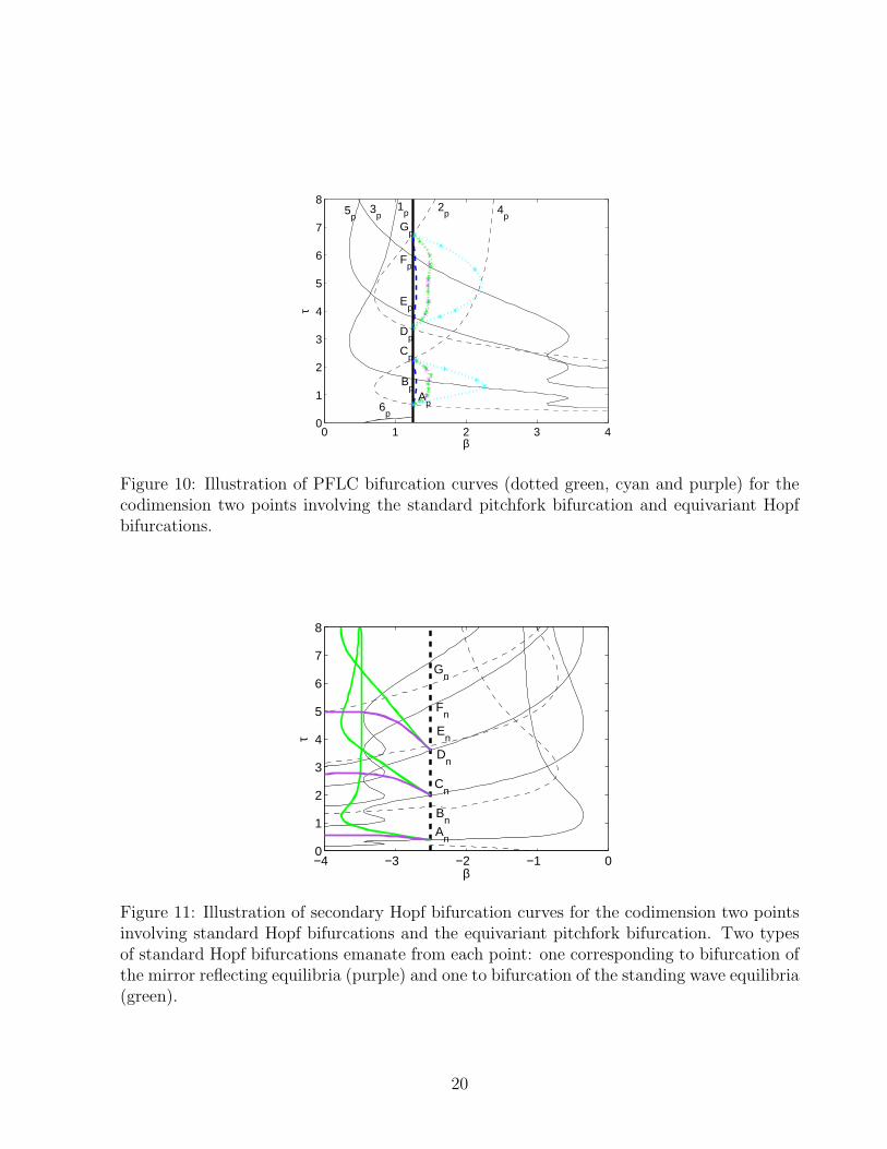
bifurcations do exist, as shown in Fig. 11. Two curves of standard Hopf bifurcations emanate

from each codimension two point. These lead, respectively, to synchronous oscillations about

the six mirror reflecting equilibria and the six standing wave equilibria. Furthermore, the

branches of synchronous oscillations about nontrivial asynchronous equilibria formed by these

18

0 0.5 1 1.5 2 2.5−3

−2

−1

0

1

2

3

β

1/3[

max

(x1)+

max

(x2)+

max

(x3)]

PL about zeroMR about zero

SW about zero

H PF

SH

MR about sync

SW about sync

PFLC

MR about zero

PL about sync

(a)

-1

1

X1

-1

1

X2

-1

1

X3

(b)

Figure 9: (a) Illustration of numerical continuation of solution branches showing pitchforkof limit cycle bifurcations for branches of asynchronous oscillations about a nontrivial syn-chronous equilibrium (τ = 1.5317). (b) An example of multistability. At β=1.3, τ=1.8 twonontrivial synchronous equilibrium points and a phase-locked oscillation about the trivialsolution are all stable.

19

0 1 2 3 40

1

2

3

4

5

6

7

8

β

τ

4p

2p

1p3

p5p

6p

Ap

Bp

Cp

Dp

Ep

Fp

Gp

Figure 10: Illustration of PFLC bifurcation curves (dotted green, cyan and purple) for thecodimension two points involving the standard pitchfork bifurcation and equivariant Hopfbifurcations.

−4 −3 −2 −1 00

1

2

3

4

5

6

7

8

β

τ

An

Bn

Cn

Dn

En

Fn

Gn

Figure 11: Illustration of secondary Hopf bifurcation curves for the codimension two pointsinvolving standard Hopf bifurcations and the equivariant pitchfork bifurcation. Two typesof standard Hopf bifurcations emanate from each point: one corresponding to bifurcation ofthe mirror reflecting equilibria (purple) and one to bifurcation of the standing wave equilibria(green).

20

secondary bifurcations end in pitchfork bifurcations of limit cycles as in the positive β case.

This is illustrated in Fig. 12. This figure shows a typical bifurcation sequence with τ held

−4 −3.5 −3 −2.5 −2−2.5

−2

−1.5

−1

−0.5

0

0.5

1

1.5

2

2.5

β

max

(x1)

PF H

SH PFLC

SW

MR

sync about SW sync about MR

Figure 12: Illustration of numerical continuation of solution branches showing pitchforklimit cycle bifurcations for synchronous oscillations about nontrivial asynchronous equilibria(τ = 0.41318).

fixed near the codimension two point and β is varied. This sequence is as follows. A standard

Hopf bifurcation (H) gives rise to a stable synchronous oscillation about the trivial solution.

The resulting unstable trivial solution undergoes an equivariant pitchfork (PF) bifurcation

to produce 12 branches of nontrivial asynchronous equilibria (six each of standing-wave and

mirror-reflecting type), which are initially unstable. These nontrivial equilibria quickly un-

dergo secondary Hopf (SH) bifurcations to produce unstable synchronous periodic solutions

about the nontrivial equilibria, which themselves become stable in the case of standing-wave

equilibria. Finally, the branches of synchronous oscillations undergo pitchfork of limit cycle

(PFLC) bifurcations which destabilize the synchronous oscillation originally created at the

Hopf point. Again, we note a region of multistability, this time between the limit cycle about

the trivial solution, and the standing-wave equilibria. The curves formed by the PFLC points

are shown in Fig. 13.

For the equivariant Hopf/equivariant pitchfork interaction points, we know of no normal

21

−4 −3 −2 −1 00

1

2

3

4

5

6

7

8

β

τ

An

Bn

Cn

Dn

En

Fn

Gn

(a)

−4 −3 −2 −1 00

1

2

3

4

5

6

7

8

β

τ

An

Bn

Cn

Dn

En

Fn

Gn

(b)

Figure 13: Illustration of PFLC bifurcation curves for codimension two points involvingstandard Hopf bifurcations and the equivariant pitchfork bifurcation. (a) PFLC bifurca-tion of synchronous oscillations about standing wave equilibria (dotted green). (b) PFLCbifurcation of synchronous oscillations about mirror reflecting equilibria (dotted purple).

form results. From Theorem 5, we predict that there are six branches of standing-wave equi-

libria and six branches of mirror-reflecting equilibria created by the pitchfork bifurcation,

and from Theorem 7 that each branch may undergo a standard Hopf bifurcation leading to

a branch of standing wave oscillations. Other standard Hopf bifurcations are also possible,

but we are not able to predict their type. It is thus reasonable to conjecture that there are

at least 12 curves of secondary standard Hopf bifurcations, leading to standing wave oscil-

lations about each of asynchronous equilibria, emanating from the codimension two points.

Note from the discussion of the characteristic equations (9)–(10), that all the standing wave

equilibria must undergo a Hopf bifurcation at the same time and similarly for the mirror

reflecting equilibria. Thus we expect that the six curves corresponding to the standing wave

equilibria will be coincident and similarly for the mirror reflecting equilibria. Evidence to

support this conjecture is shown in Fig. 14 where numerically computed secondary Hopf

curves for equivariant Hopf / equivariant pitchfork interaction points are shown. Here, just

22

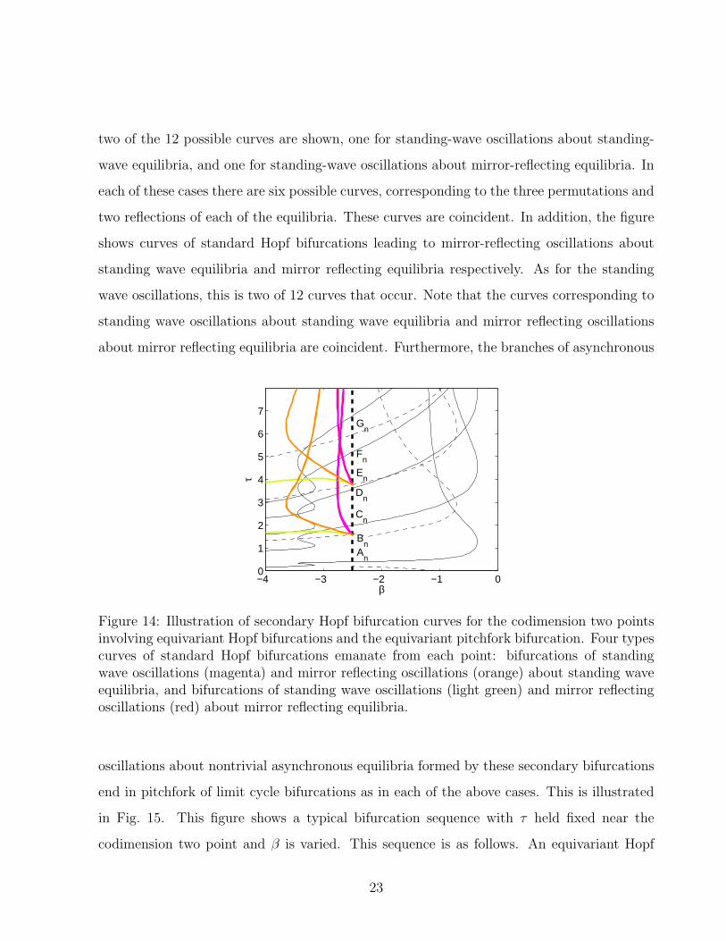
two of the 12 possible curves are shown, one for standing-wave oscillations about standing-

wave equilibria, and one for standing-wave oscillations about mirror-reflecting equilibria. In

each of these cases there are six possible curves, corresponding to the three permutations and

two reflections of each of the equilibria. These curves are coincident. In addition, the figure

shows curves of standard Hopf bifurcations leading to mirror-reflecting oscillations about

standing wave equilibria and mirror reflecting equilibria respectively. As for the standing

wave oscillations, this is two of 12 curves that occur. Note that the curves corresponding to

standing wave oscillations about standing wave equilibria and mirror reflecting oscillations

about mirror reflecting equilibria are coincident. Furthermore, the branches of asynchronous

−4 −3 −2 −1 00

1

2

3

4

5

6

7

β

τ

An

Bn

Cn

Dn

En

Fn

Gn

Figure 14: Illustration of secondary Hopf bifurcation curves for the codimension two pointsinvolving equivariant Hopf bifurcations and the equivariant pitchfork bifurcation. Four typescurves of standard Hopf bifurcations emanate from each point: bifurcations of standingwave oscillations (magenta) and mirror reflecting oscillations (orange) about standing waveequilibria, and bifurcations of standing wave oscillations (light green) and mirror reflectingoscillations (red) about mirror reflecting equilibria.

oscillations about nontrivial asynchronous equilibria formed by these secondary bifurcations

end in pitchfork of limit cycle bifurcations as in each of the above cases. This is illustrated

in Fig. 15. This figure shows a typical bifurcation sequence with τ held fixed near the

codimension two point and β is varied. This sequence is as follows. An equivariant Hopf

23

(H) bifurcation gives rise to an unstable asynchronous oscillation (mirror-reflecting in this

case) about the trivial solution. Subsequently, the unstable trivial solution undergoes an

equivariant pitchfork (PF) bifurcation to produce 12 branches of nontrivial asynchronous

equilibria (standing-wave shown), which are initially unstable. These nontrivial equilibria

undergo secondary equivariant Hopf (SH) bifurcations to produce unstable asynchronous

periodic solutions about the nontrivial equilibria (MR about SW shown). Here, the branch

of mirror-reflecting oscillations about the standing-wave equilibrium is subcritical and ends

in a pitchfork of limit cycles bifurcation. PFLC points for equivariant Hopf, equivariant

−4 −3 −2 −1 0−3

−2

−1

0

1

2

3

β

max

(x1)

H

PF

SH

PFLC

SW

MR about SW

MR about zero

Figure 15: Illustration of numerical continuation of solution branches showing a pitchfork oflimit cycles bifurcation for a branch of mirror-reflecting oscillations about a standing-waveequilibrium (τ = 4). Note that the trivial solution became unstable in a standard Hopfbifurcation near β = −0.5.

pitchfork interactions are shown in Fig. 16. Again, the PFLC curves are created by fitting

splines through these points. In the case of standing-wave oscillations about mirror-reflecting

equilibria (light green curves), the spline was fit to the PFLC points as well as the maxi-

mum point of the secondary Hopf curves since it was found that periodic solution branches

continued from points beyond this extremum were supercritical (unlike those prior to the

extremum), and did not terminate in a PFLC bifurcation.

We close this section by noting that the secondary Hopf bifurcations emanating from the

24

−4 −3.5 −3 −2.5 −2 −1.5 −1 −0.5 00

1

2

3

4

5

6

7

8

β

τ

A

B

C

D

E

F

G

H

(a)

−4 −3 −2 −1 00

1

2

3

4

5

6

7

β

τ

Cn

An

Bn

Dn

En

Fn

Gn

(b)

Figure 16: Illustration of PFLC bifurcation curves for the codimension two points involvingequivariant Hopf bifurcations and the equivariant pitchfork bifurcation. (a) PFLC bifurca-tion of asynchronous oscillations about standing wave equilibria (dotted magenta and or-ange). (b) PFLC bifurcation of asynchronous oscillations about mirror reflecting equilibria(dotted red and light green).

25

various codimension two bifurcation points in our model (1) lead to many different patterns

of oscillation. Some examples are shown in Fig. 17. Of these, we have only found parameter

values where two of these are stable: the synchronous oscillations about the trivial solution

and the standing wave oscillations about the trivial solution. As discussed above, these

patterns are a result of the many interactions of the standard and equivariant steady state

(pitchfork) bifurcations with the standard and equivariant Hopf bifurcations exhibited by

the model.

4 Discussion

We have studied, via numerical continuation, the 4 types of codimension two Hopf-pitchfork

interactions exhibited by (1). In the case where both bifurcations are standard, our numer-

ical results agree qualitatively with the predictions of normal form theory. There are two

secondary bifurcation branches emanating from each codimension two point: a Hopf bifurca-

tion of limit cycles surrounding the nontrivial equilibria and a pitchfork bifurcation of these

limit cycles. This agreement could be checked quantitatively by using a centre manifold

reduction of the delay differential equation as was done for a standard Hopf pitchfork inter-

action in Belair et al. [1996]. In the remaining three cases, one or more of the bifurcations is

equivariant. We know of no normal form results for these situations, thus we summarize our

results with some conjectures about what normal form analysis may tell us. Although we

considered a ring of three oscillators, based on our analysis of the bifurcations of the trivial

solution [Yuan and Campbell, 2004; Campbell et al., 2005] we know that all the codimension

two points observed here are also observed in the case of n oscillators. We thus state our

conjectures for Dn symmetric systems.

Conjecture 8: Consider a codimension two bifurcation point involving a standard pitchfork

bifurcation and a Dn equivariant Hopf bifurcation of an equilibrium point. There will be a

secondary equivariant Hopf bifurcation emanating from the codimension two point, giving

rise to 2n + 2 branches of periodic orbits (n standing wave oscillations, n mirror reflecting

26

0 0.2 0.4 0.6 0.8 1−0.5

0

0.5

1

1.5

t/T

x 1, x2, x

3

0 0.2 0.4 0.6 0.8 1−2

−1.5

−1

−0.5

0

0.5

1

t/T

x 1, x2, x

3

0 0.2 0.4 0.6 0.8 1−1.5

−1

−0.5

0

0.5

1

1.5

t/T

x 1,x2,x

3

0 0.2 0.4 0.6 0.8 1−0.4

−0.3

−0.2

−0.1

0

0.1

0.2

0.3

0.4

t/T

x 1, x2, x

3

0 0.2 0.4 0.6 0.8 1−2.5

−2

−1.5

−1

−0.5

0

0.5

1

t/T

x 1, x2, x

3

0 0.2 0.4 0.6 0.8 1−0.4

−0.3

−0.2

−0.1

0

0.1

0.2

0.3

0.4

t/T

x 1, x2, x

3

Figure 17: Illustration of the various patterns of oscillation about nontrivial equilibria ex-hibited by (1). From top left clockwise: synchronous oscillation about a synchronous equi-librium, standing-wave oscillation about a synchronous equilibrium, mirror-reflecting oscil-lation about a standing-wave equilibrium, standing-wave oscillation about a standing-waveequilibrium, mirror-reflecting oscillation about a mirror-reflecting equilibrium, synchronousoscillation about a standing-wave equilibrium.

27

oscillations and 2 phase-locked oscillations) about each equilibria produced by the pitchfork

bifurcation. There will also be 2n + 2 pitchfork bifurcations of limit cycles emanating from

the codimension two point.

Conjecture 9: Consider a codimension two bifurcation point involving a Dn equivariant

pitchfork bifurcation and a standard Hopf bifurcation of an equilibrium point. Note that

the pitchfork bifurcation gives rise to 2n standing wave equilibria and 2n mirror reflect-

ing equilibria. There will be 4n secondary standard Hopf bifurcations emanating from the

codimension two point, giving rise to 4n synchronous periodic orbits, one about each of

the 4n asynchronous equilibria. There will also be 2n pitchfork bifurcations of limit cycles

emanating from the codimension two point.

Conjecture 10: Consider a codimension two bifurcation point involving a Dn equivariant

pitchfork bifurcation and a Dn equivariant Hopf bifurcation of an equilibrium point. There

will be 8n secondary standard Hopf bifurcations emanating from the codimension two point,

giving rise to 8n branches of periodic orbits, two about each of the 4n equilibria produced

by the equivariant pitchfork bifurcation. There will also be 4n pitchfork bifurcations of limit

cycles.

Although we studied a specific type of oscillator in our ring, we believe that these general

results should carry over to other symmetric rings of type II oscillators (i.e. the inherent

oscillations are induced by a supercritical Hopf bifurcation) with time delayed coupling of

the form we use here. Bifurcation diagrams similar to those we obtain are found in Buric

et al. [2005] and Buric and Todorovic [2003] when studying Fitzhugh-Nagumo oscillators and

in Campbell et al. [2004] when studying simple loop oscillators with time delayed coupling.

Returning to the neural system, it would seem that the choice of oscillator model we

made makes the synchronous oscillations about the trivial solution fairly robust. The many

other types of oscillations possible in this network are, for the most part, unstable. This

might be a desirable property for a network which needs to reliably produce a particular

oscillation for a range of parameters. As indicated above, we believe that using other type II

28

oscillator models will give similar results, namely the secondary bifurcations will be the same.

However, the locations and criticality of these secondary bifurcations may well change. In

particular, it may be possible to produce systems where the secondary bifurcations produce

stable oscillations of different patterns. This would lead to a network which has flexibility:

changes to parameters can cause a large change in the response of the system.

References

Baldi, P. and Atiya, A. F. (1994). How delays affect neural dynamics and learning. IEEE

Trans. Neural Networks, 5(4):612–621.

Belair, J. and Campbell, S. A. (1994). Stability and bifurcations of equilibria in a multiple-

delayed differential equation. SIAM J. Appl. Math., 54(5):1402–1424.

Belair, J., Campbell, S. A., and van den Driessche, P. (1996). Frustration, stability and

delay-induced oscillations in a neural network model. SIAM J. Appl. Math., 56:245–255.

Buric, N., Grozdanovic, I., and Vasovic, N. (2005). Type I vs. type II excitable systems with

delayed coupling. Chaos Solitons Fractals, 23:1221–1233.

Buric, N. and Todorovic, D. (2003). Dynamics of Fitzhugh-Nagumo excitable systems with

delayed coupling. Phys. Rev. E, 67:066222.

Campbell, S. A. (1999). Stability and bifurcation of a simple neural network with multiple

time delays. In Ruan, S., Wolkowicz, G. S. K., and Wu, J., editors, Differential equations

with application to biology, Fields Institute Communications, volume 21, pages 65–79.

AMS.

Campbell, S. A., Edwards, R., and van den Driessche, P. (2004). Delayed coupling between

two neural network loops. SIAM J. Appl. Math., 65(1):316–335.

Campbell, S. A., Ncube, I., and Wu, J. (2006). Multistability and stable asynchronous

periodic oscillations in a multiple-delayed neural system. Phys. D, 214(2):101–119.

29

Campbell, S. A., Ruan, S., and Wei, J. (1999). Qualitative analysis of a neural network

model with multiple time delays. Internat. J. Bifur. Chaos, 9(8):1585–1595.

Campbell, S. A., Yuan, Y., and Bungay, S. D. (2005). Equivariant Hopf bifurcation in a ring

of identical cells with delayed coupling. Nonlinearity, 18:2827–2846.

Cohen, M. and Grossberg, S. (1983). Absolute stability of global pattern formation and

parallel memory storage by competitive neural networks. IEEE Trans. Systems Man

Cybernet., 13(5):815–826.

Dhooge, A., Govaerts, W., and Kuznetsov, Y. A. (2003). Matcont: A matlab pack-

age for numerical bifurcation analysis of ODEs. ACM Trans. Math. Soft., 29:141–164.

www.matcont.ugent.be.

Doedel, E. J., Keller, H. B., and Kernevez, J. P. (1991a). Numerical analysis and control

of bifurcation problems, (I) Bifurcation in finite dimensions. Internat. J. Bifur. Chaos,

1(3):493–520.

Doedel, E. J., Keller, H. B., and Kernevez, J. P. (1991b). Numerical analysis and control

of bifurcation problems, (II) Bifurcation in infinite dimensions. Internat. J. Bifur. Chaos,

1(4):745–772.

Engelborghs, K., Luzyanina, T., and Samaey, G. (2001). DDE-BIFTOOL v. 2.00: a Matlab

package for bifurcation analysis of delay differential equations. Technical Report TW-330,

Department of Computer Science, K. U. Leuven, Leuven, Belgium.

Ermentrout, B. (2002). Simulating, analyzing, and animating dynamical systems: A guide

to XPPAUT for researchers and students. SIAM, Philadelphia.

Golubitsky, M., Stewart, I., and Schaeffer, D. G. (1988). Singularities and groups in bifur-

cation theory, volume 2. Springer Verlag, New York.

Grossberg, S. (1978). Competition, decision, and consensus. J. Math. Anal. Appl., 66(2):470–

493.

30

Grossberg, S. (1980). Biological competition: Decision rules, pattern formation, and oscilla-

tions. Proc. Nat. Acad. Sci. USA, 77(4):2338–2342.

Guckenheimer, J. and Holmes, P. J. (1983). Nonlinear oscillations, dynamical systems and

bifurcations of vector fields. Springer-Verlag, New York.

Guo, S. (2005). Spatio-temporal patterns of nonlinear oscillations in an excitatory ring

network with delay. Nonlinearity, 18:2391–2407.

Guo, S. and Huang, L. (2003). Hopf bifurcating periodic orbits in a ring of neurons with

delays. Phys. D, 183:19–44.

Guo, S. and Huang, L. (2005). Global continuation of nonlinear waves in a ring of neurons.

Proc. Roy. Soc. Edinburgh, 135A:999–1015.

Guo, S. and Huang, L. (2006). Nonlinear waves in a ring of neurons with delays. IMA J.

Appl. Math. (to appear).

Guo, S., Huang, L., and Wang, L. (2004). Linear stability and Hopf bifurcation in a two

neuron network with three delays. Internat. J. Bifur. Chaos, 14:2799–2810.

Hale, J. K. and Lunel, V. (1993). Introduction to functional differential equations. Springer

Verlag, New York.

Hopfield, J. J. (1982). Neural networks and physical systems with emergent collective com-

putational abilities. Proc. Nat. Acad. Sci. USA, 79(8):2554–2558.

Hopfield, J. J. (1984). Neurons with graded response have collective computational properties

like those of two-state neurons. Proc. Nat. Acad. Sci. USA, 81:3088–3092.

Krawcewicz, W., Vivi, P., and Wu, J. (1997). Computation formulae of an equivariant degree

with applications to symmetric bifurcations. Nonlinear Stud., 4(1):89–119.

31

Krawcewicz, W. and Wu, J. (1999). Theory and applications of Hopf bifurcations in

symmetric functional-differential equations. Nonlinear Anal., 35(7, Series A: Theory

Methods):845–870.

Kuznetsov, Y. A. (1995). Elements of applied bifurcation theory. Springer-Verlag, Berlin/New

York.

Marcus, C. M., Waugh, F. R., and Westervelt, R. M. (1991). Nonlinear dynamics and

stability of analog neural networks. Phys. D, 51:234–247.

Marcus, C. M. and Westervelt, R. M. (1989). Stability of analog neural networks with delay.

Phys. Rev. A, 39(1):347–359.

Ncube, I., Campbell, S. A., and Wu, J. (2003). Change in criticality of synchronous Hopf

bifurcation in a multiple-delayed neural system. Fields Inst. Commun., 36:17–193.

Orosz, G., Krauskopf, B., and Wilson, R. E. (2005). Bifurcations and multiple traffic jams

in a car-following model with reaction-time delay. Phys. D, 211(3):277–293.

Orosz, G. and Stepan, G. (2004). Hopf bifurcation calculations in delayed systems with

translational symmetry. J. Nonlinear Sci., 14(6):505–528.

Orosz, G. and Stepan, G. (2006). Subcritical Hopf bifurcations in a car-following model with

reaction-time delay. Proc. Roy. Soc. London A. (to appear).

Orosz, G., Wilson, R. E., and Krauskopf, B. (2004). Global bifurcation investigation of an

optimal velocity traffic model with driver reaction time. Phys. Rev. E, 70(2):026207.

Shayer, L. P. and Campbell, S. A. (2000). Stability, bifurcation and multistability in a system

of two coupled neurons with multiple time delays. SIAM J. Appl. Math., 61(2):673–700.

Wu, J. (1998). Symmetric functional-differential equations and neural networks with memory.

Trans. Amer. Math. Soc., 350(12):4799–4838.

32

Wu, J., Faria, T., , and Huang, Y. S. (1999). Synchronization and stable phase-locking in a

network of neurons with memory. Math. Comput. Modelling, 30(1–2):117–138.

Yuan, Y. and Campbell, S. A. (2004). Stability and synchronization of a ring of identical

cells with delayed coupling. J. Dynam. Differential Equations, 16(1):709–744.

33

A Line Style and Colour Convention

Primary bifurcationsBifurcation / Oscillation Equilibrium Line style Colourstandard Hopf trivial solid blackequivariant Hopf trivial dashed blackstandard pitchfork trivial solid (wide) blackequivariant pitchfork trivial dashed (wide) black

Secondary bifurcationsBifurcation / Oscillation Equilibrium Line style Colourstandard Hopf / sync sync solid blueequivariant Hopf / PL,SW,MR sync dashed bluestandard Hopf / sync SW solid greenstandard Hopf / sync MR solid purplestandard Hopf / SW SW solid magentastandard Hopf / SW MR solid light greenstandard Hopf / MR SW solid orangestandard Hopf / MR MR solid redPFLC / sync sync dotted bluePFLC / MR sync dotted purplePFLC / SW sync dotted greenPFLC / PL sync dotted cyan

Table 1: The line style and colour convention used for the bifurcation curves. The line style isdetermined by the type of bifurcation, while the line colour is determined by a combination ofthe type of oscillation and the type of equilibrium about which the oscillations are produced.

34