PATTERN RECOGNITION ANDMACHINE LEARNING

Slide Set 1: Introduction and the Basics of Python

January 2018

Heikki Huttunenheikki.huttunen@tut.fi

Laboratory of Signal ProcessingTampere University of Technology

Course Organization

� Organized on 3rd period; January – February 2018.

� Lectures every Monday 10-12 (RI207) and Wednesday 12-14 (RI207).

� 10 groups of exercises (sign up at POP).

� More details: http://www.cs.tut.fi/courses/SGN-41007/

Course Requirements

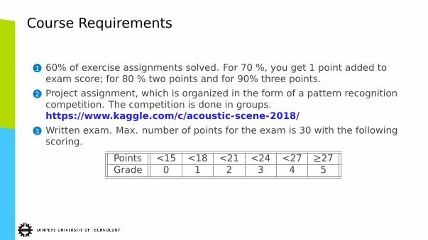
1 60% of exercise assignments solved. For 70 %, you get 1 point added toexam score; for 80 % two points and for 90% three points.

2 Project assignment, which is organized in the form of a pattern recognitioncompetition. The competition is done in groups.https://www.kaggle.com/c/acoustic-scene-2018/

3 Written exam. Max. number of points for the exam is 30 with the followingscoring.

Points <15 <18 <21 <24 <27 ≥27Grade 0 1 2 3 4 5

Course Contents

1 Python: Rapidly becoming the default platform for practical machinelearning

2 Estimation of Signal Parameters: What are the phase, amplitude andfrequency of this noisy sinusoid

3 Detection Theory: Detect whether there is a specific signal present or not4 Performance evaluation: Cross-Validation, Bootstrapping, Receiver

Operating Characteristics, other Error Metrics5 Machine Learning Models: Logistic Regression, Support Vector Machine,

Random Forests, Deep Learning6 Avoid Overlearning and Solve Ill-Posed Problems: Regularization

Techniques

Introduction

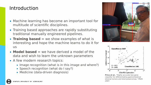
� Machine learning has become an important tool formultitude of scientific disciplines.

� Training based approaches are rapidly substitutingtraditional manually engineered pipelines.

� Training based = we show examples of what isinteresting and hope the machine learns to do it forus

� Model based = we have derived a model of thedata and wish to learn the unknown parameters

� A few modern research topics:� Image recognition (what is in this image and where?)� Speech recognition (what do I say?)� Medicine (data-driven diagnosis)

Price et al., "Highly accurate two-geneclassifier for differentiating gastrointestinalstromal tumors and leiomyosarcomas," PNAS2007.

Why Python?

� Python is becoming increasingly central tool fordata science.

� This was not always the case: 10 years agoeveryone was using Matlab.

� However, due to licensing issues and heavydevelopment of Python, scientific Pythonstarted to gain its user base.

� Python’s strength is in its variability and hugecommunity.

� There are 2 versions: Python 2.7 and 3.6. We’lluse the latter.

Source: Kaggle.com newsletter, Dec. 2016

Alternatives to Python in SciencePython vs. Matlab Python vs. R

� Matlab is #1 workhorse for linearalgebra.

� Matlab is professionally maintainedproduct.

� Some Matlab’s toolboxes are great(Image Processing tb). Some areobsolete (Neural Network tb).

� New versions twice a year. Amount ofnovelty varies.

� Matlab is expensive fornon-educational users.

� R has been #1 workhorse for statisticsand data analysis. a

� R is great for specific data analysis andvisualization needs.

� Lots of statistics community code in R.

� Python interfaces with other domainsranging from deep neural networks(Tensorflow, pyTorch) and imageanalysis (OpenCV) to even a fullblownwebserver (Django/Flask)

ahttp://tinyurl.com/jynezuq

� "Matlab is made for mathematicians, R for statisticians and Python forprogrammers."

Essential Modules

� numpy: The matrix / numerical analysis layer at the bottom� scipy: Scientific computing utilities (linalg, FFT, signal/image processing...)� scikit-learn: Machine learning (our focus here)� matplotlib: Plotting and visualization� opencv: Computer vision� pandas: Data analysis� statsmodels: Statistics in Python� Tensorflow, keras: Deep learning� PyCharm: Editor� spyder: Scientific PYthon Development EnviRonment (another editor)

Where to get Python?

� It is possible to construct your custom Python environment by installingindividual modules (base from python.org and libraries from, e.g.,http://www.lfd.uci.edu/~gohlke/pythonlibs/).

� Alternatively, one may install a full distribution, such as� Anaconda https://www.anaconda.com/download/ ← my favorite� Enthought Canopy http://www.enthought.com/

� ...or in linux:# apt-get install python# apt-get install python-numpy# apt-get install python-sklearn# apt-get install python-matplotlib# apt-get install spyder

The Language

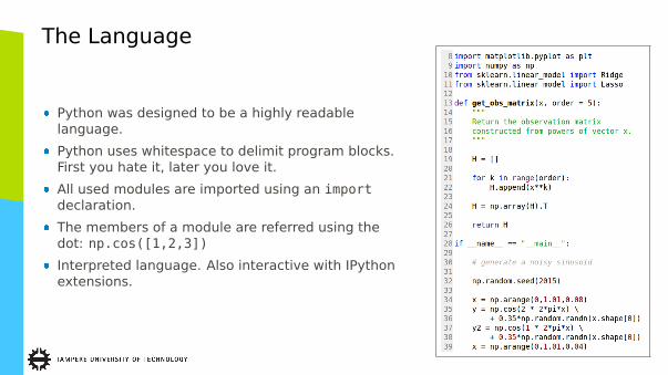
� Python was designed to be a highly readablelanguage.

� Python uses whitespace to delimit program blocks.First you hate it, later you love it.

� All used modules are imported using an importdeclaration.

� The members of a module are referred using thedot: np.cos([1,2,3])

� Interpreted language. Also interactive with IPythonextensions.

Things to Come

� Following slides will introduce the basic Python usage within scientificcomputing.

� The editor and the environment� Matlab slightly better than Python

� Linear algebra� Matlab better than Python

� Programming constructs (loops, classes, etc.)� Python better than Matlab

� Machine learning� Python a lot better than Matlab

Editors� In this course we use theSpyder and PyCharm editors.

� Spyder comes with Anaconda,PyCharm you install on yourown. TC303 exercise class hasPyCharm.

� Spyder window contains twopanes: editor on the left andconsole on the right.

� F5 : Run code; F9 : Runselected region.

� Alternatively, you can usewhatever editor you like, andrun everything on thecommand line.

Python Basics

� Python code can be executed eitherfrom a script file (*.py) or in theinteractive mode (just like Matlab).

� For the interactive mode; just executepython from the command line.

� Alternatively, ipython (if installed)starts Python in a more user-friendlymode:

� Tab-completion works� Many utility functions (e.g., ls, pwd, cd)� Magic functions (e.g., %run, %timeit,%edit, %pastebin)

Command range creates a list ofintegers. Compare to Matlab’s syntax1:2:6.

Help

� For each command, help is there to refresh your memory:>>> help("".strip) # strip is a member of the string classHelp on built-in function strip:

strip(...)S.strip([chars]) -> string or unicode

Return a copy of the string S with leading and trailingwhitespace removed.If chars is given and not None, remove characters in chars instead.If chars is unicode, S will be converted to unicode before stripping

� In ipython, the shortcut ? is available, too (see previous slide).� Many people prefer to Google for python strip instead; matter of taste.

Using Modules

� Python libraries are called modules.� Each module needs to be imported before

use.� Three common alternatives:

1 Import the full module: import numpy2 Import selected functions from the module:

from numpy import array, sin, cos3 Import all functions from the module:

from numpy import *

>>> sin(pi)

NameError: name ’sin’ is not defined

>>> from numpy import sin, pi

>>> sin(pi)1.2246467991473532e-16

>>> import numpy as np

>>> np.sin(np.pi)1.2246467991473532e-16

>>> from numpy import *

>>> sin(pi)1.2246467991473532e-16

Using Modules

A few things to note:� All methods support shortcuts; e.g.,import numpy as np.

� Sometimes import <module> fails, if themodule is in fact a collection of modules.For example, import scipy. Instead, useimport scipy.signal

� Importing all functions from the module isnot recommended, because differentmodules may contain functions with thesame name.

>>> import scipy

>>> matfile = scipy.io.loadmat("myfile.mat")

AttributeError: ’module’ object has no attribute ’io’

>>> import scipy.io as sio

>>> matfile = sio.loadmat("myfile.mat") # Works OK

>>> from scipy.io import loadmat

>>> matfile = loadmat("myfile.mat") # Works OK

NumPy

� Practically all scientific computing in Pythonis based on numpy and scipy modules.

� NumPy provides a numerical array as analternative to Python list.

� The list type is very generic and acceptsany mixture of data types.

� Although practical for genericmanipulation, it is becomes inefficient incomputing.

� Instead, the NumPy array is more limitedand more focused on numerical computing.

# Python list accepts any data typesv = [1, 2, 3, "hello", None]

# We like to call numpy briefly "np">>> import numpy as np

# Define a numpy array (vector):>>> v = np.array([1, 2, 3, 4])

# Note: the above actually casts a# Python list into a numpy array.

# Resize into 2x2 matrix>>> V = np.resize(v, (2, 2))

# Invert:>>> np.linalg.inv(V)array([[-2. , 1. ],

[ 1.5, -0.5]])

More on Vectors

� np.arange creates a range array (like 1:0.5:10 in Matlab)>>> np.arange(1, 10, 0.5) # Arguments: (start, end, step)array([ 1. , 1.5, 2. , 2.5, 3. , 3.5, 4. , 4.5, 5. , 5.5, 6. ,

6.5, 7. , 7.5, 8. , 8.5, 9. , 9.5])

# Note that the endpoint is not included (unlike Matlab).

� Most vector/matrix functions are similar to Matlab:>>> np.linspace(1, 10, 5) # Arguments: (start, end, num_items)array([ 1. , 3.25, 5.5 , 7.75, 10. ])

>>> np.eye(3)array([[ 1., 0., 0.],

[ 0., 1., 0.],[ 0., 0., 1.]])

>>> np.random.randn(2, 3)array([[-2.23506417, 0.47311746, 0.05343861],

[ 1.255074 , -0.03576461, 0.96121907]])

Matrices

� A matrix is defined similarly; either by specifying the values manually, orusing special functions.# A matrix is simply an array of arrays# May seem complicated at first, but is in fact# nice for N-D arrays.

>>> np.array([[1, 2], [3, 4]])array([[1, 2],

[3, 4]])

>>> from scipy.linalg import toeplitz, hilbert # You could also " ...import *">>> toeplitz([3, 1, -2])array([[ 3, 1, -2],

[ 1, 3, 1],[-2, 1, 3]])

>>> hilbert(3)array([[ 1. , 0.5 , 0.33333333],

[ 0.5 , 0.33333333, 0.25 ],[ 0.33333333, 0.25 , 0.2 ]])

Matrix Product

� Matrix multiplication is differentfrom Matlab. Use np.dot ornp.matmul.

� With NumPy version 1.10+ andPython 3.5+, matrix multiplicationcan be done with the @ operator:A @ B.

>>> A = np.array([[1, 2], [3, 4]])>>> B = np.array([[5, 6], [7, 8]])

>>> A * B # Elementwise product (Matlab: A .* B)array([[ 5, 12],

[21, 32]])

>>> np.dot(A, B) # Matrix product; alternatively: np.matmularray([[19, 22],

[43, 50]])

$ python3Python 3.5.2 (default, Nov 17 2016, 17:05:23)>>> import numpy as np>>> A = np.random.rand(3,3)>>> B = np.random.rand(3,3)>>> A @ Barray([[ 0.28382296, 0.90172558, 1.10036663],

[ 0.39959554, 1.12141386, 1.39473854],[ 0.28797509, 0.82918235, 1.04229714]])

Indexing

� Indexing of vectors uses the colon notation, too.� Below, we extract selected items from the vector 1...10:

>>> x = np.arange(1, 11)>>> x[0:8:2] # Unlike Matlab, indexing starts from 0array([1, 3, 5, 7])

# Note: use square brackets for indexing# Note2: colon operator has the order start:end:step;# not start:step:end as in Matlab

� The start and end points can be omitted:>>> x[5:] # All items from the 5’tharray([ 6, 7, 8, 9, 10])>>> x[:5] # All items until the 5’tharray([1, 2, 3, 4, 5])>>> x[::3] # All items with step 3array([ 1, 4, 7, 10])

Indexing

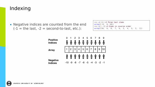
� Negative indices are counted from the end(-1 = the last, -2 = second-to-last, etc.):

>>> x[-3:] # Three last itemsarray([ 8, 9, 10])>>> x[::-1] # Items in inverse orderarray([10, 9, 8, 7, 6, 5, 4, 3, 2, 1])

Indexing

� Also matrices can be indexed similarly. This operation is called slicing, andthe result is a slice of the matrix.

� Here we request for items on the rows2:4 = [2,3] and columns 1,2,4 (shown inred).

� Note, that with matrices, the first index isthe row; not "x-coordinate".

� This order is called "Fortran style" or"column major" while the alternative is"C style" or "row major".

>>> M = np.reshape(np.arange(0, 36), (6, 6))array([[ 0, 1, 2, 3, 4, 5],

[ 6, 7, 8, 9, 10, 11],[12, 13, 14, 15, 16, 17],[18, 19, 20, 21, 22, 23],[24, 25, 26, 27, 28, 29],[30, 31, 32, 33, 34, 35]])

>>> M[2:4, [1,2,4]]array([[13, 14, 16],

[19, 20, 22]])

Indexing

� To specify only column or row indices, use ":" alone.

� Now we wish to extract two bottom rows.� M[4:, :] reads "give me all rows after the

4th and all columns".� In this case, alternative forms would be,e.g., M[-2:, :] and M[[4,5], :].

>>> M = np.reshape(np.arange(0, 36), (6, 6))array([[ 0, 1, 2, 3, 4, 5],

[ 6, 7, 8, 9, 10, 11],[12, 13, 14, 15, 16, 17],[18, 19, 20, 21, 22, 23],[24, 25, 26, 27, 28, 29],[30, 31, 32, 33, 34, 35]])

>>> M[4:, :]array([[24, 25, 26, 27, 28, 29],

[30, 31, 32, 33, 34, 35]])

N-Dimensional arrays

� Higher-dimensional arrays are frequentlyencountered in machine learning.

� For example, a set of 1000 color images of sizew× h = 128× 96 is represented as a1000× 3× 96× 128 array.

� Here, dimensions are: image index, colorchannel, y-coordinate, x-coordinate.

� Sometimes, a shorter name is used:"(b, c, 0, 1) order".

# Generate a random "image" array:>>> A = np.random.rand(1000, 3, 96, 128)

# What size is it?>>> A.shape(1000L, 3L, 96L, 128L)

# Access the pixel (4, 3) of 2nd color channel# of the 2nd image>>> A[1, 2, 3, 4]0.36569219631994954

# Request all color channels:>>> A[1, :, 3, 4]array([ 0.32306666, 0.60012626, 0.3656922 ])

# Request a complete 96x128 color channel:>>> A[1, 2, :, :]array([[ 0.19102217 ...0.88464718]])

# Equivalent shorter notation:>>> A[1, 2, ...]array([[ 0.19102217 ...0.88464718]])

Functions

� Functions are defined using the defkeyword.

� Function definition can appearanywhere in the code.

� Functions can be imported to other filesusing import.

� Function arguments can be positionalor named (see code).

� Named arguments improve readabilityand are handy for setting the lastargument in a long list.

# Define our first functiondef hello(target):

print ("Hello " + target + "!")

>>> hello("world")Hello world!

>>> hello("Finland")Hello Finland!

# We can also define the default argument:def hello(target = "world"):

print ("Hello " + target + "!")

>>> hello()Hello world!

>>> hello("Finland")Hello Finland!

# One can also assign using the name:

>>> hello(target = "Finland")Hello Finland!

Loops and Stufffor lang in [’Assembler’, ’Python’, "Matlab", ’C++’]:

if lang in ["Assembler", "C++"]:print ("I am ok with %s." % (lang))

else:print ("I love %s." % (lang))

I am ok with Assembler.I love Python.I love Matlab.I am ok with C++.

# Read all lines of a file until the end

fp = open("myfile.txt", "r")lines = []

while True:

try:line = fp.readline()lines.append(line)

except:# File endedbreak

fp.close()

� Loops and other usualprogramming constructs areeasy to remember.

� for can loop over anythingiterable, such as a list or a file.

� In Matlab, appending values toa vector in a loop is notrecommended. Python lists areactual lists, so appending isfine.

Example: Reading in a Data File

� Suppose we need to read a csv file(text file with Comma SeparatedValues) into Python.

� The file consists of 216 rows (samples) with 4000 measurements each.� We will write file reading code from scratch.� Alternatively, many modules contain csv-reading functions

� numpy.loadtxt or numpy.genfromtxt� csv.reader� pandas.read_csv

Example: Reading in a Data File

import numpy as np

if __name__ == "__main__":

X = [] # Rows of the file go here

# We use Python’s with statement.# Then we do not have to worry# about closing it.

with open("ovarian.csv", "r") as fp:

# File is iterable, so we can# read it directly (instead of# using readline).

for line in fp:

# Skip the first line:if "Sample_ID" in line:

continue

# Otherwise, split the line# to numbers:values = line.split(";")

# Omit the first item# ("S1" or similar):values = values[1:]

# Cast each item from# string to float:values = [float(v) for v in values]

# Append to XX.append(values)

# Now, X is a list of lists. Cast to# Numpy array:X = np.array(X)

print ("All data read.")print ("Result size is %s" % (str(X.shape)))

Visualization

import matplotlib.pyplot as pltimport numpy as np

N = 100n = np.arange(N) # Vector [0,1,2,...,N-1]x = np.cos(2 * np.pi * n * 0.03)x_noisy = x + 0.2 * np.random.randn(N)

fig = plt.figure(figsize = [10,5])

plt.plot(n, x, ’r-’,linewidth = 2,label = "Clean Sinusoid")

plt.plot(n, x_noisy, ’bo-’,markerfacecolor = "green",label = "Noisy Sinusoid")

plt.grid("on")plt.xlabel("Time in $\mu$s")plt.ylabel("Amplitude")plt.title("An Example Plot")plt.legend(loc = "upper left")

plt.show()plt.savefig("../images/sinusoid.pdf",

bbox_inches = "tight")

� The matplotlib module is our plotting library.� Function names are often similar to Matlab.� Usually you want to

"import matplotlib.pyplot".� Alternatively, "from matplotlib.pylabimport *" makes the environment very similarto Matlab.

� Code also inhttps://github.com/mahehu/SGN-41007

0 20 40 60 80 100Time in µs

1.5

1.0

0.5

0.0

0.5

1.0

1.5

Am

plit

ude

An Example Plot

Clean SinusoidNoisy Sinusoid

Another Example

� Even rather complicatedgraphics are easy togenerate using Matplotlib.

� The code for the attacheddiagram is shown inhttps://github.com/mahehu/SGN-41007.

HackerSkills Substance

Math & Statistics

Danger Zone

Model Based Research(Biology, Physics,...)Machine Learning

Superman