Pattern Recognition

Pattern Recognition and Machine Learning

Eunho Lee

2017-01-03(Tue)

January 8, 2017 1 / 33

Outline

1 IntroductionPolynomial Curve FittingProbability TheoryThe Curse of DimensionalityDecision TheoryInformation Theory

2 Appendix C - Properties of MatricesDeterminantsMatrix Derivatives2.3. Eigenvector Equation

January 8, 2017 2 / 33

Introduction

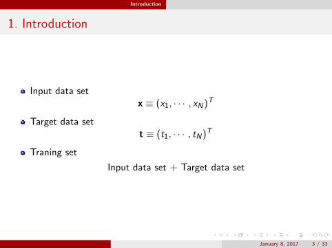
1. Introduction

Input data setx ≡ (x1, · · · , xN)T

Target data sett ≡ (t1, · · · , tN)T

Traning set

Input data set + Target data set

January 8, 2017 3 / 33

Introduction

1. Introduction

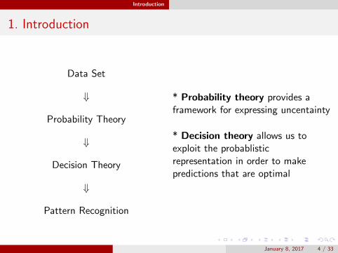
Data Set

⇓

Probability Theory

⇓

Decision Theory

⇓

Pattern Recognition

* Probability theory provides aframework for expressing uncentainty

* Decision theory allows us toexploit the probablisticrepresentation in order to makepredictions that are optimal

January 8, 2017 4 / 33

Introduction Polynomial Curve Fitting

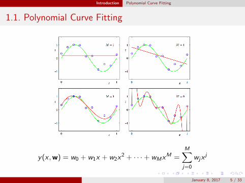
1.1. Polynomial Curve Fitting

y(x ,w) = w0 + w1x + w2x2 + · · ·+ wMxM =

M∑j=0

wjxj

January 8, 2017 5 / 33


1.1. Polynomial Curve Fitting1.1.1. Error Functions

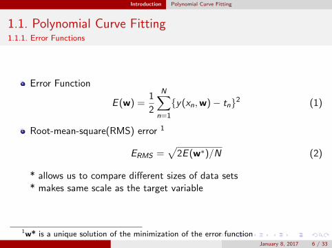
Error Function

E (w) =1

2

N∑n=1

{y(xn,w)− tn}2 (1)

Root-mean-square(RMS) error 1

ERMS =√

2E (w∗)/N (2)

* allows us to compare different sizes of data sets* makes same scale as the target variable

1w* is a unique solution of the minimization of the error functionJanuary 8, 2017 6 / 33


1.1. Polynomial Curve Fitting1.1.2. Over-Fitting

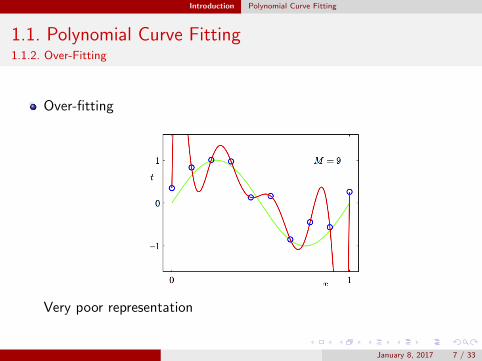
Over-fitting

Very poor representation

January 8, 2017 7 / 33


1.1. Polynomial Curve Fitting1.1.3. Modified Error Function

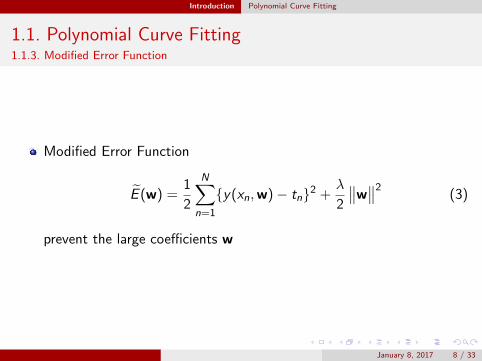
Modified Error Function

E (w) =1

2

N∑n=1

{y(xn,w)− tn}2 +λ

2

∥∥w∥∥2 (3)

prevent the large coefficients w

January 8, 2017 8 / 33

Introduction Probability Theory

1.2. Probability Theory

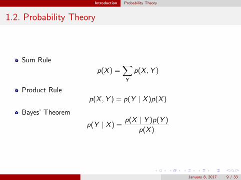
Sum Rule

p(X ) =∑Y

p(X ,Y )

Product Rulep(X ,Y ) = p(Y | X )p(X )

Bayes’ Theorem

p(Y | X ) =p(X | Y )p(Y )

p(X )

January 8, 2017 9 / 33


1.2. Probability Theory

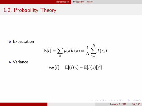
Expectation

E[f ] =∑x

p(x)f (x) ' 1

N

N∑n=1

f (xn)

Variancevar [f ] = E[(f (x)− E[f (x)])2]

January 8, 2017 10 / 33


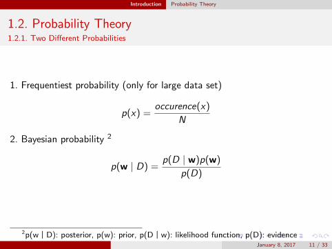
1.2. Probability Theory1.2.1. Two Different Probabilities

1. Frequentiest probability (only for large data set)

p(x) =occurence(x)

N

2. Bayesian probability 2

p(w | D) =p(D | w)p(w)

p(D)

2p(wㅣD): posterior, p(w): prior, p(Dㅣw): likelihood function, p(D): evidenceJanuary 8, 2017 11 / 33


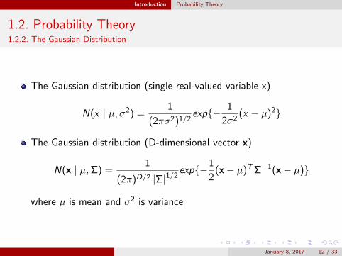
1.2. Probability Theory1.2.2. The Gaussian Distribution

The Gaussian distribution (single real-valued variable x)

N(x | µ, σ2) =1

(2πσ2)1/2exp{− 1

2σ2(x − µ)2}

The Gaussian distribution (D-dimensional vector x)

N(x | µ,Σ) =1

(2π)D/2 |Σ|1/2exp{−1

2(x− µ)TΣ−1(x− µ)}

where µ is mean and σ2 is variance

January 8, 2017 12 / 33



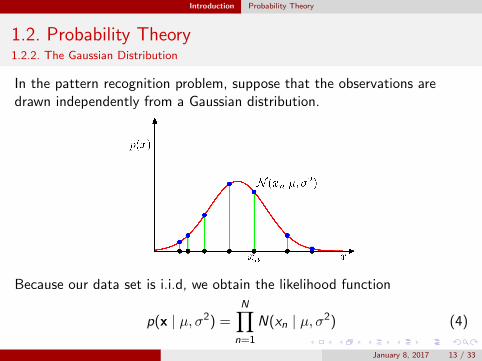
In the pattern recognition problem, suppose that the observations aredrawn independently from a Gaussian distribution.

Because our data set is i.i.d, we obtain the likelihood function

p(x | µ, σ2) =N∏

n=1

N(xn | µ, σ2) (4)

January 8, 2017 13 / 33



Our goal is to find µML, σ2ML which maximize the likelihood function (4).

Take log for convenience,

ln p(x | µ, σ2) = − 1

2σ2

N∑n=1

(xn − µ)2 − N

2lnσ2 − N

2ln (2π) (5)

From (5) with respect to µ,

µML =1

N

N∑n=1

xn (sample mean)

Similarly, with respect to σ2,

σ2ML =1

N

N∑n=1

(xn − µML)2 (sample variance)

January 8, 2017 14 / 33



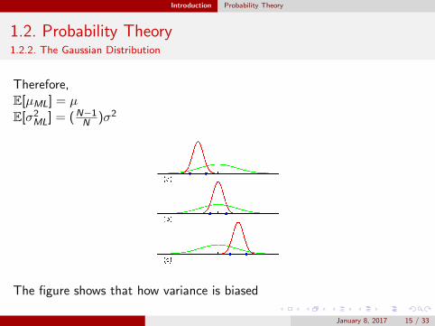
Therefore,E[µML] = µE[σ2ML] = (N−1

N )σ2

The figure shows that how variance is biased

January 8, 2017 15 / 33


1.2. Probability Theory1.2.3. Curve Fitting (re-visited)

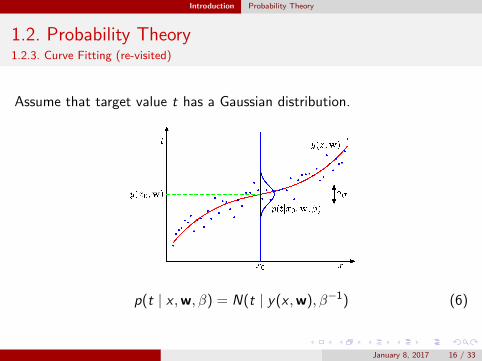
Assume that target value t has a Gaussian distribution.

p(t | x ,w, β) = N(t | y(x ,w), β−1) (6)

January 8, 2017 16 / 33



Because the data are drawn independently, the likelihood is given by

p(t | x,w, β) =N∏

n=1

N(tn | y(xn,w), β−1) (7)

1. Maximum Likelihood Function MethodOur goal is to maximize the likelihood function (7).Take log for convenience,

ln p(t | x,w, β) = −β2

N∑n=1

{y(xn,w)− tn}2 +N

2lnβ − N

2ln (2π) (8)

January 8, 2017 17 / 33



Maximizing (8) with respect to w is equivalent to minimizing thesum-of-squares error function (1)

Maximizing (5) with respect to β gives

1

βML=

1

N

N∑n=1

{y(xn,wML)− tn}2

January 8, 2017 18 / 33



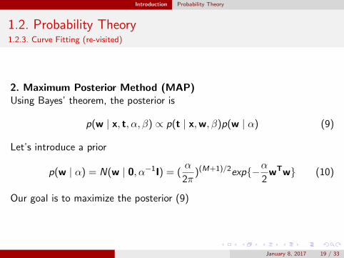
2. Maximum Posterior Method (MAP)Using Bayes’ theorem, the posterior is

p(w | x, t, α, β) ∝ p(t | x,w, β)p(w | α) (9)

Let’s introduce a prior

p(w | α) = N(w | 0, α−1I) = (α

2π)(M+1)/2exp{−α

2wTw} (10)

Our goal is to maximize the posterior (9)

January 8, 2017 19 / 33



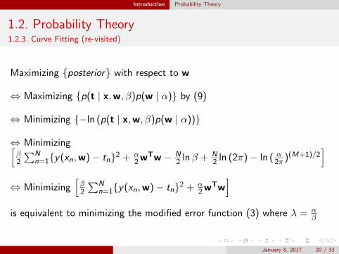
Maximizing {posterior} with respect to w

⇔ Maximizing {p(t | x,w, β)p(w | α)} by (9)

⇔ Minimizing {−ln (p(t | x,w, β)p(w | α))}

⇔ Minimizing[β2

∑Nn=1{y(xn,w)− tn}2 + α

2 wTw − N2 lnβ + N

2 ln (2π)− ln ( α2π )(M+1)/2]

⇔ Minimizing[β2

∑Nn=1{y(xn,w)− tn}2 + α

2 wTw]

is equivalent to minimizing the modified error function (3) where λ = αβ

January 8, 2017 20 / 33


1.2. Probability Theory1.2.4. Bayesian Curve Fitting

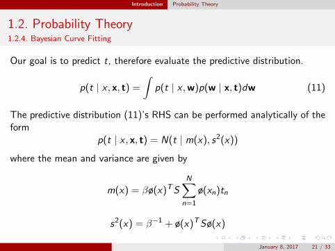
Our goal is to predict t, therefore evaluate the predictive distribution.

p(t | x , x, t) =

∫p(t | x ,w)p(w | x, t)dw (11)

The predictive distribution (11)’s RHS can be performed analytically of theform

p(t | x , x, t) = N(t | m(x), s2(x))

where the mean and variance are given by

m(x) = βø(x)TSN∑

n=1

ø(xn)tn

s2(x) = β−1 + ø(x)TSø(x)

January 8, 2017 21 / 33

Introduction The Curse of Dimensionality

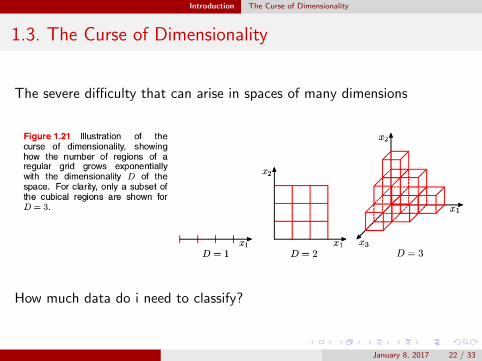
1.3. The Curse of Dimensionality

The severe difficulty that can arise in spaces of many dimensions

How much data do i need to classify?

January 8, 2017 22 / 33

Introduction Decision Theory

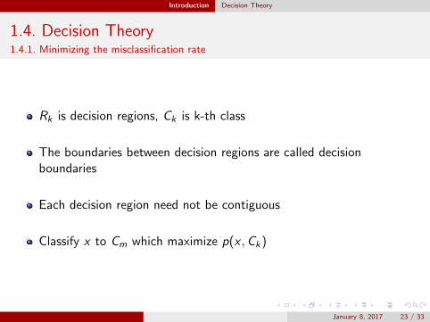
1.4. Decision Theory1.4.1. Minimizing the misclassification rate

Rk is decision regions, Ck is k-th class

The boundaries between decision regions are called decisionboundaries

Each decision region need not be contiguous

Classify x to Cm which maximize p(x ,Ck)

January 8, 2017 23 / 33


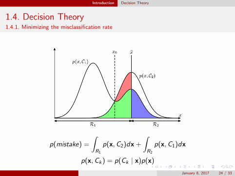
1.4. Decision Theory1.4.1. Minimizing the misclassification rate

p(mistake) =

∫R1

p(x,C2)dx +

∫R2

p(x,C1)dx

p(x,Ck) = p(Ck | x)p(x)

January 8, 2017 24 / 33


1.4. Decision Theory1.4.2. Minimizing the expected loss

Dicision’s value is different each other

Minimize the expected loss by using the loss matrix L

E[L] =∑k

∑j

∫Rj

Lkjp(x,Ck)dx

January 8, 2017 25 / 33


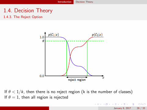
1.4. Decision Theory1.4.3. The Reject Option

If θ < 1/k , then there is no reject region (k is the number of classes)If θ = 1, then all region is rejected

January 8, 2017 26 / 33

Introduction Information Theory

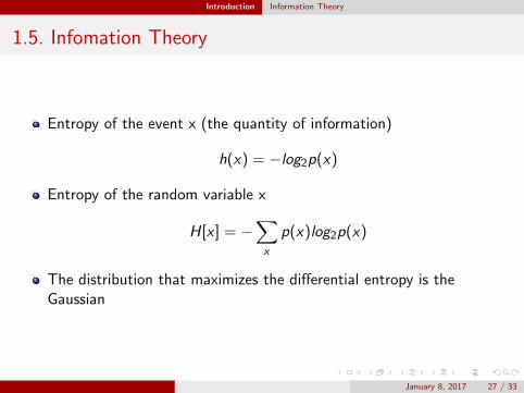
1.5. Infomation Theory

Entropy of the event x (the quantity of information)

h(x) = −log2p(x)

Entropy of the random variable x

H[x ] = −∑x

p(x)log2p(x)

The distribution that maximizes the differential entropy is theGaussian

January 8, 2017 27 / 33

Appendix C - Properties of Matrices

2. Appendix C - Properties of Matrices

Determinants

Matrix Derivatives

Eigenvector Equation

January 8, 2017 28 / 33

Appendix C - Properties of Matrices Determinants

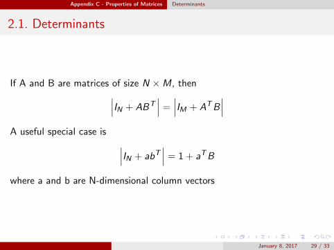
2.1. Determinants

If A and B are matrices of size N ×M, then∣∣∣IN + ABT∣∣∣ =

∣∣∣IM + ATB∣∣∣

A useful special case is ∣∣∣IN + abT∣∣∣ = 1 + aTB

where a and b are N-dimensional column vectors

January 8, 2017 29 / 33

Appendix C - Properties of Matrices Matrix Derivatives

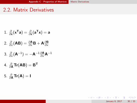
2.2. Matrix Derivatives

1. ∂∂x (xTa) = ∂

∂x (aTx) = a

2. ∂∂x (AB) = ∂A

∂x B + A∂B∂x

3. ∂∂x (A−1) = −A−1 ∂A

∂x A−1

4. ∂∂ATr(AB) = BT

5. ∂∂ATr(A) = I

January 8, 2017 30 / 33

Appendix C - Properties of Matrices Eigenvector Equation

2.3. Eigenvector Equation

For a square matrix A, the eigenvector equation is defined by

Aui = λiui

where ui is an eigenvector and λi is the corresponding eigenvalue

January 8, 2017 31 / 33



If A is diagonalized, we can say that

A = UΛUT

By using that equation, we obtain

1. |A| =∏M

i=1 λi

2. Tr(A) =∑M

i=1 λi

January 8, 2017 32 / 33



1. The eigenvalues of symmetirc matrices are real

2. The eigenvectors ui statisfies

uTi uj = Iij

January 8, 2017 33 / 33

Pattern Recognition

Data & Analytics

Transcript of Pattern Recognition