Pattern Recognition

K-Nearest Neighbor ExplainedBy

Arthur EvansJohn Sikorski

Patricia Thomas

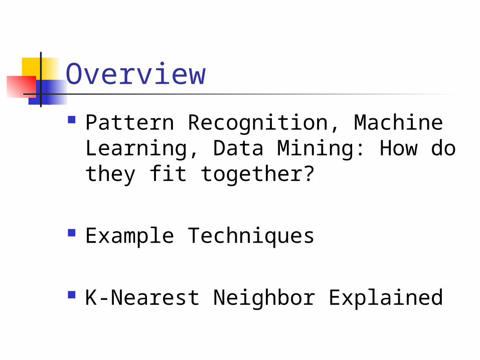
Overview Pattern Recognition, Machine

Learning, Data Mining: How do they fit together?

Example Techniques

K-Nearest Neighbor Explained

Data Mining Searching through electronically

stored data in an automatic way Solving problems with already

known data Essentially, discovering patterns in

data Has several subsets from statistics

to machine learning

Machine Learning Construct computer programs that

improve with use A methodology Draws from many fields: Statistics,

Information Theory, Biology, Philosophy, Computer Science . . .

Several sub-disciplines: Feature Extraction, Pattern Recognition

Pattern recognition Operation and design of systems

that detect patterns in data The algorithmic process Applications include image

analysis, character recognition, speech analysis, and machine diagnostics.

Pattern Recognition Process

Gather data Determine features to use Extract features Train your recognition engine Classify new instances

Artificial Neural Networks

A type of artificial intelligence that attempts to imitate the way a human brain works.

Creates connections between processing elements, computer equivalent of neurons

Supervised technique

ANN continued Tolerant of errors in data

Many applications: speech recognition, analyze visual scenes, robot control

Best at interpreting complex real world sensor data.

The Brain Human brain has about 1011 neurons Each connect to about 104 other neurons Switch in about 10-3 seconds

Slow compared to a computers at 10-13

seconds Brain recognizes a familiar face in about 10-1

seconds Only 200-300 cycles at its switch rate

Brain utilizes MASSIVE parallel processing, considers many factors at once.

Neural Network Diagram

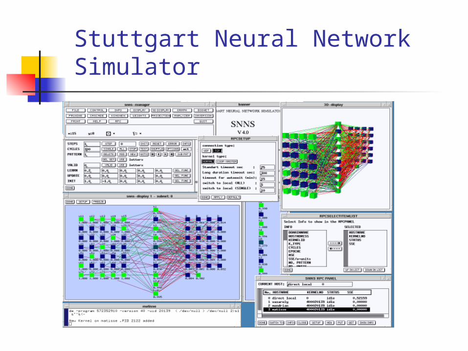
Stuttgart Neural Network Simulator

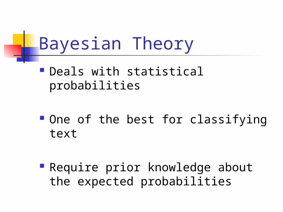
Bayesian Theory Deals with statistical probabilities

One of the best for classifying text

Require prior knowledge about the expected probabilities

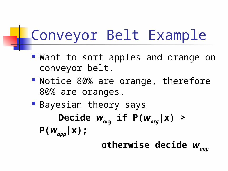
Conveyor Belt Example Want to sort apples and orange on

conveyor belt. Notice 80% are orange, therefore

80% are oranges. Bayesian theory says Decide worg if P(worg|x) > P(wapp|x);

otherwise decide wapp

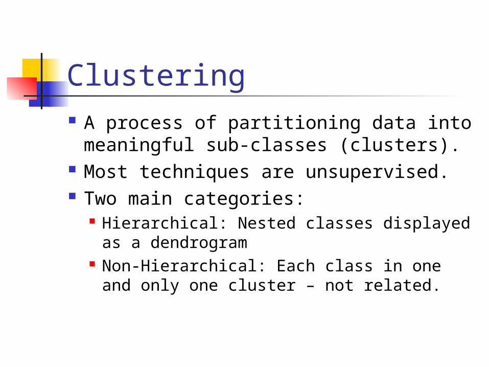
Clustering A process of partitioning data into

meaningful sub-classes (clusters). Most techniques are unsupervised. Two main categories:

Hierarchical: Nested classes displayed as a dendrogram

Non-Hierarchical: Each class in one and only one cluster – not related.

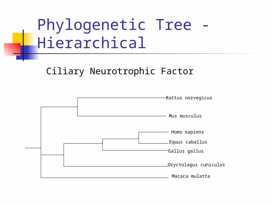
Phylogenetic Tree - Hierarchical

Rattus norvegicus

Mus musculus

Homo sapiens

Equus caballus

Gallus gallus

Oryctolagus cuniculus

Macaca mulatta

Ciliary Neurotrophic Factor

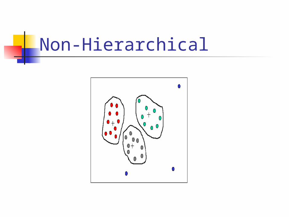
Non-Hierarchical

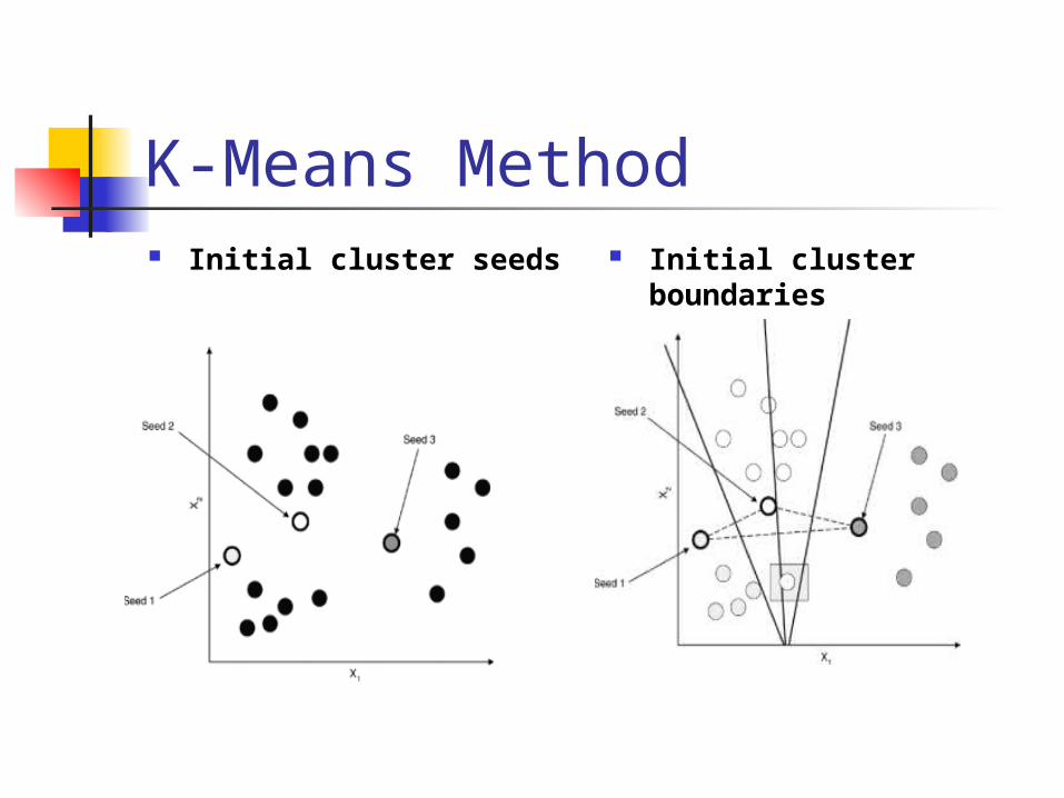
K-Means Method Initial cluster seeds Initial cluster

boundaries

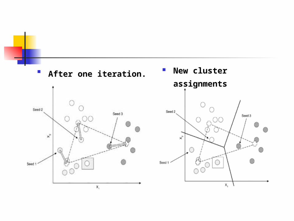
After one iteration. New cluster

assignments

Decision Tree A flow-chart-like tree structure Internal node denotes a test on an

attribute (feature) Branch represents an outcome of the

test All records in a branch have the same

value for the tested attribute Leaf node represents class label or class

label distribution

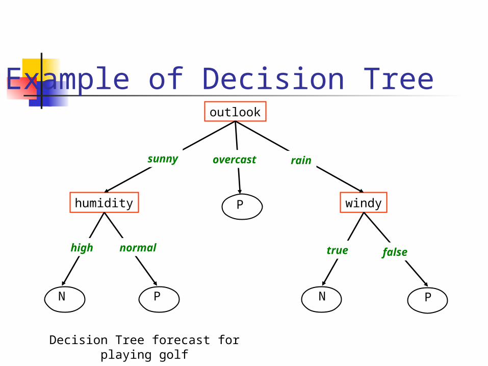
Example of Decision Treeoutlook

humidity windyP

P N PN

sunny overcast rain

high normal true false

Decision Tree forecast for playing golf

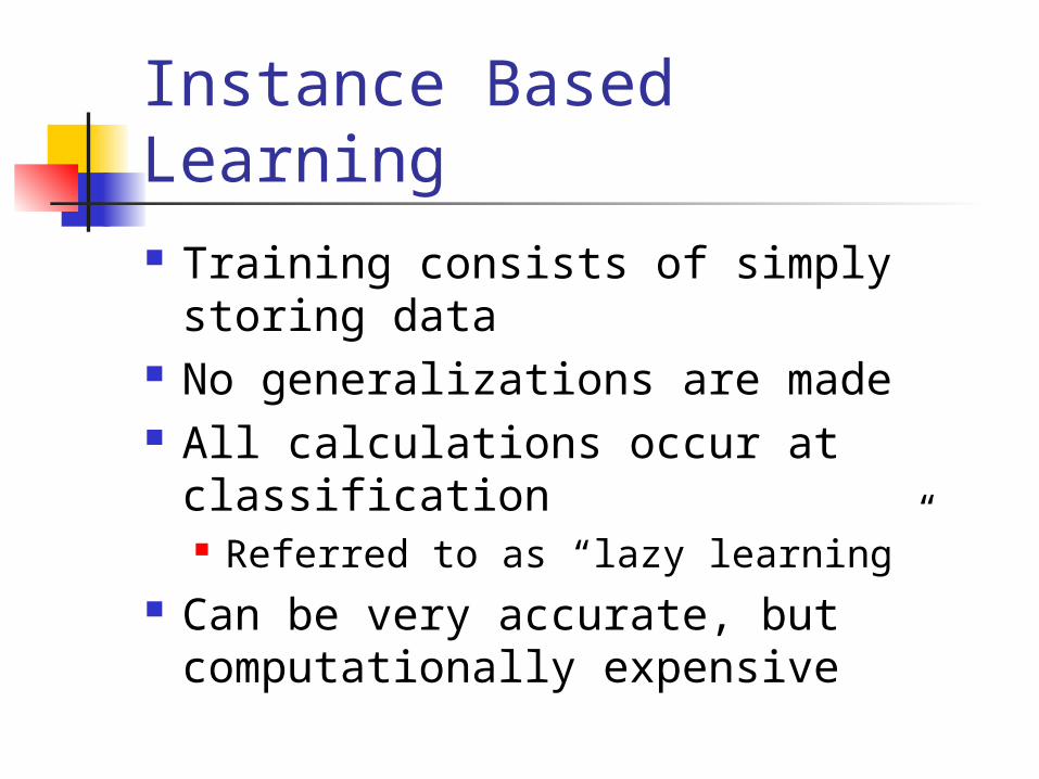
Instance Based Learning Training consists of simply storing

data No generalizations are made All calculations occur at

classification Referred to as “lazy learning”

Can be very accurate, but computationally expensive

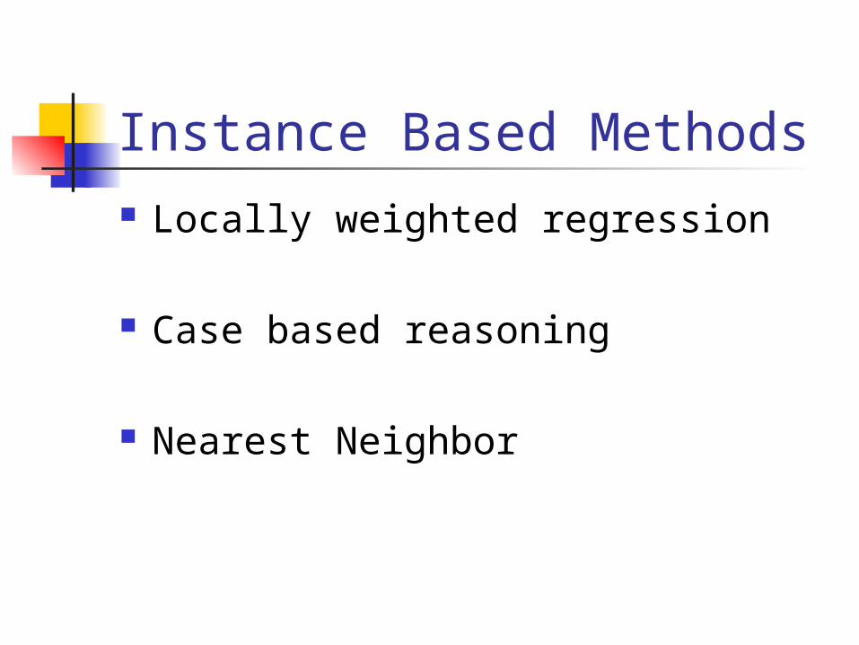
Instance Based Methods Locally weighted regression

Case based reasoning

Nearest Neighbor

Advantages Training stage is trivial therefore it

is easily adaptable to new instances Very accurate Different “features” may be used

for each classification Able to model complex data with

less complex approximations

Difficulties All processing done at query time:

computationally expensive Determining appropriate distance

metric for retrieving related instances

Irrelevant features may have a negative impact

Case Based Reasoning Does not use Euclidean space Represented as complex logical

descriptions Examples

Retrieve help desk information Legal reasoning Conceptual design of mechanical

devices

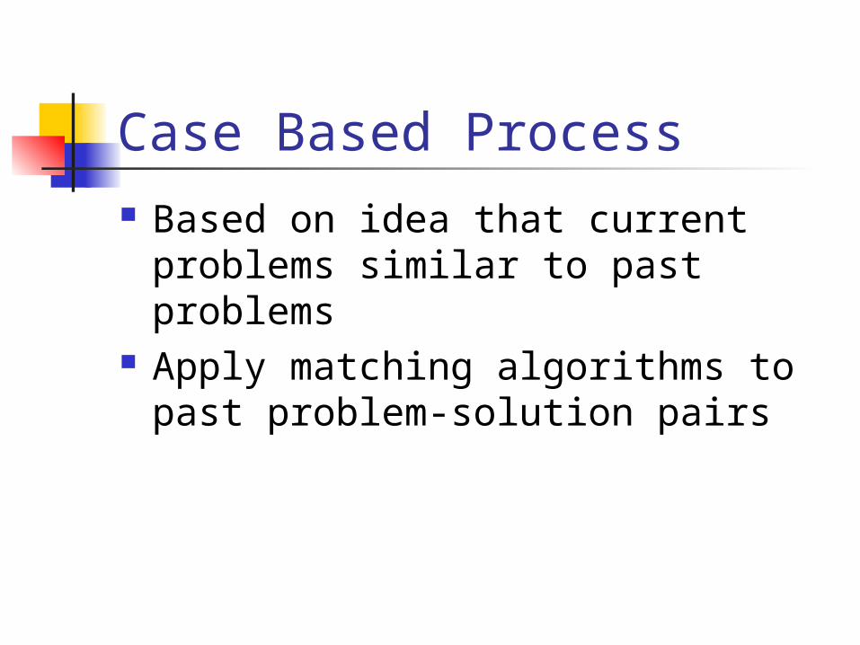
Case Based Process Based on idea that current

problems similar to past problems Apply matching algorithms to past

problem-solution pairs

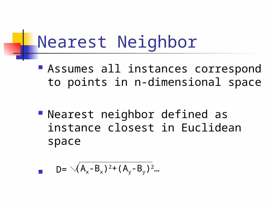
Nearest Neighbor Assumes all instances correspond

to points in n-dimensional space

Nearest neighbor defined as instance closest in Euclidean space

(Ax-Bx)2+(Ay-By)2…D=

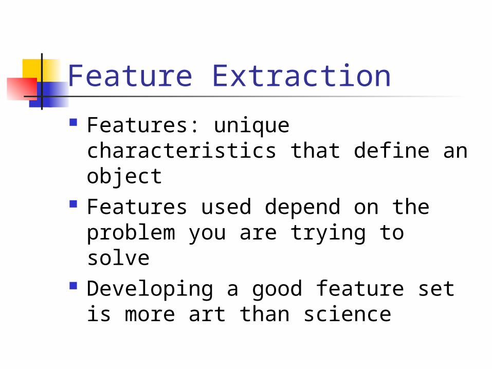
Feature Extraction Features: unique characteristics

that define an object Features used depend on the

problem you are trying to solve Developing a good feature set is

more art than science

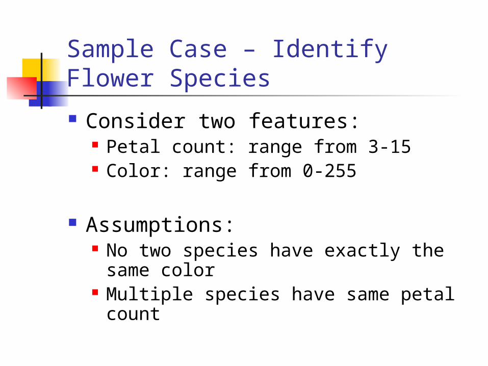
Sample Case – Identify Flower Species

Consider two features: Petal count: range from 3-15 Color: range from 0-255

Assumptions: No two species have exactly the same

color Multiple species have same petal

count

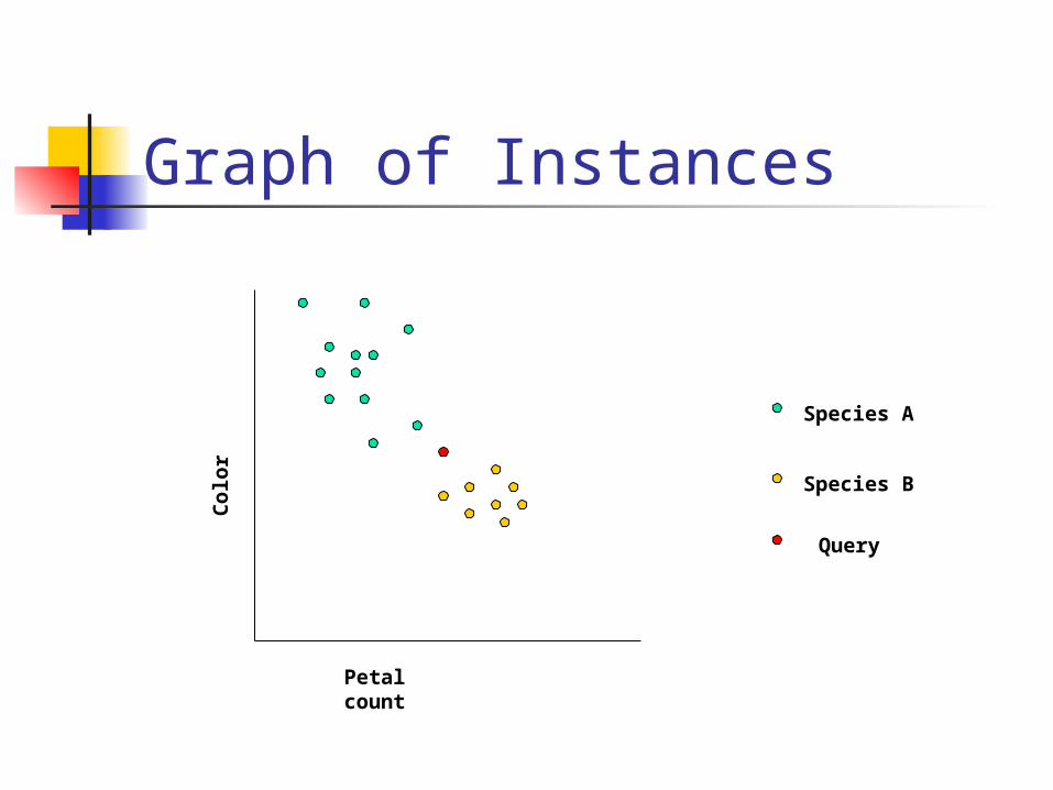
Graph of Instances

Species A

Species B

Query

Petal count

Colo

r

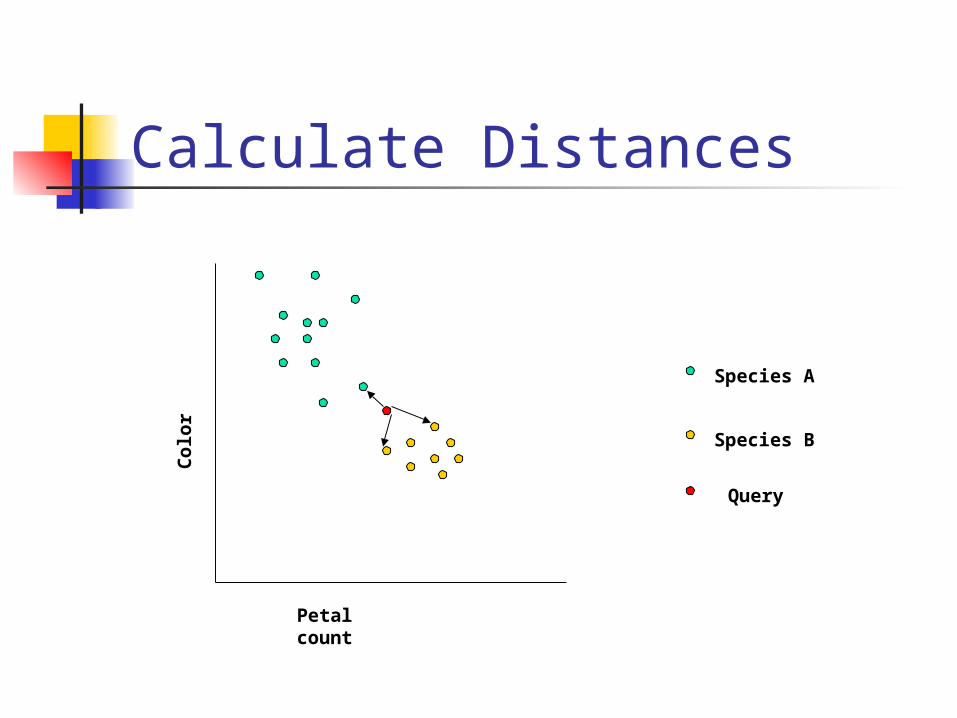
Calculate Distances

Petal count

Colo

r

Species A

Species B

Query

Species is Closest Neighbor

Petal count

Colo

r

Species A

Species B

Query

Nearest Neighbor

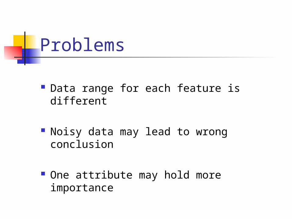
Problems

Data range for each feature is different

Noisy data may lead to wrong conclusion

One attribute may hold more importance

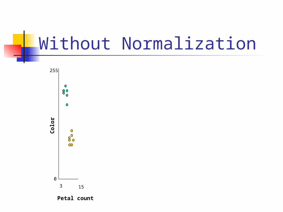
Without Normalization255

Petal count

Colo

r

0

3 15

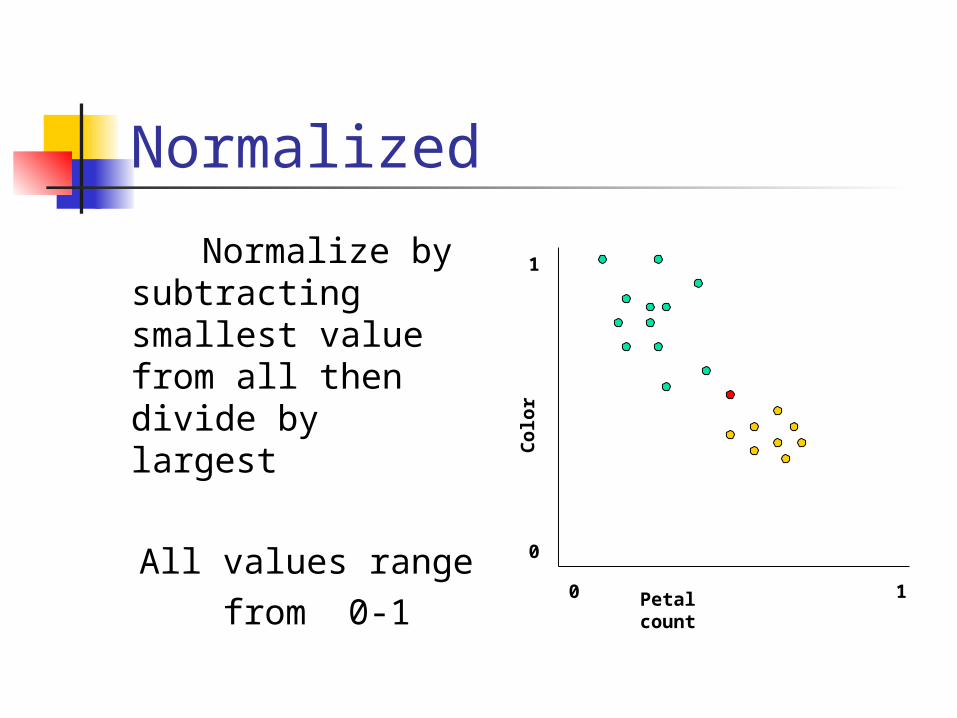
Normalized

Normalize by subtracting smallest value from all then divide by largest

All values range from 0-1 Petal

count

Colo

r0

0

1

1

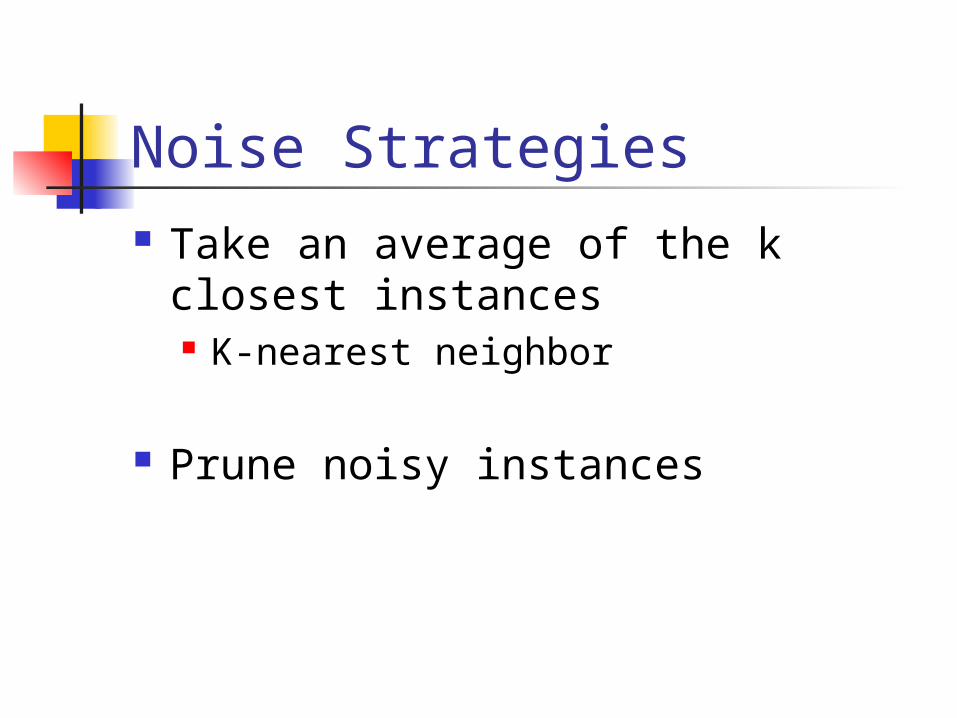
Noise Strategies Take an average of the k closest

instances K-nearest neighbor

Prune noisy instances

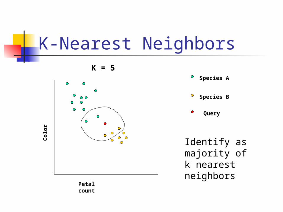
K-Nearest Neighbors

Petal count

Colo

r

K = 5

Identify as majority of k nearest neighbors

Species A

Species B

Query

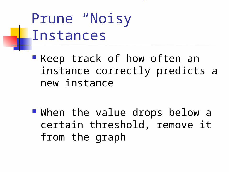
Prune “Noisy” Instances Keep track of how often an

instance correctly predicts a new instance

When the value drops below a certain threshold, remove it from the graph

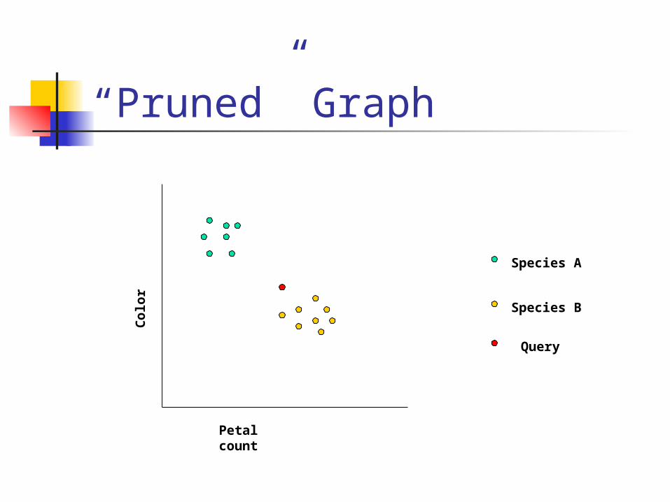
“Pruned” Graph

Petal count

Colo

r

Species A

Species B

Query

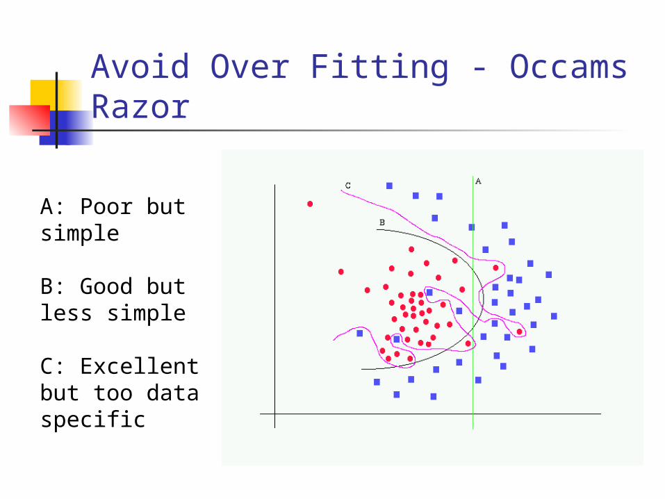
Avoid Over Fitting - Occams Razor

A: Poor but simple

B: Good but less simple

C: Excellent but too data specific

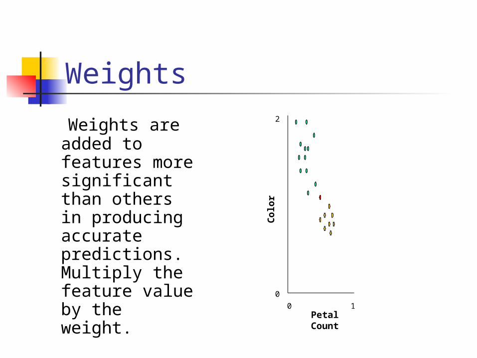
Weights

Weights are added to features more significant than others in producing accurate predictions. Multiply the feature value by the weight.

Petal Count

Colo

r

0

0 1

2

Validation Used to calculate error rates and

overall accuracy of recognition engine Leave One out: Use n-1 instances in

classifier, test, repeat n times. Holdout: Divide data into n groups,

use n-1 groups in classifier, repeat n times

Bootstrapping: Test with a randomly sampled subset of instances.

Potential Pattern Recognition Problems

Are there adequate features to distinguish different classes.

Are the features highly correlated.

Are there distinct subclasses in the data.

Is the feature space too complex.