Pattern Formation in a Simple Fluid System:

Taylor-vortex Flow

Phys. 128

Department of Physics

UCSB

Winter 2006

1

FIG. 1: Left: Cloud streets over the Arabian peninsular. Right: Permafrost stripes in Spitzbergen.

I. INTRODUCTION

In this experiment we are concerned with phenomena involving non-equilibrium non-

linear systems. By “non-equilibrium” we mean systems that are driven away from the

thermodynamic state, by the application of some stress parameter R such as a temperature

difference, a shear rate, a concentration difference, or an electric voltage. Usually this leads

to a current (for instance a heat, momentum, mass, or electrical current) passing through the

system. This current produces dissipation. Thus, our systems are typically also dissipative.

By that we mean that energy is converted at some rate, for instance by friction associated

with the viscosity in fluid flow, into heat which is lost from the macroscopic dynamics of the

system (such as the flow of a fluid). A particularly interesting aspect of nonlinear dissipative

systems driven far from equilibrium is that they may undergo transitions from a temporally

and/or spatially uniform state to a state of lower symmetry with characteristic temporal

and/or spatial variations in the properties. Such transitions are called bifurcations.

In the first part of this experiment we shall study a bifurcation in a well defined laboratory

system, namely the flow of a fluid between two concentric cylinders with the inner one

rotating. This flow is known as Taylor-vortex flow (TVF). For careful laboratory study our

system has the great virtue that it is relatively simple and that all factors influencing it

can be carefully controlled. Consequently a complete theoretical analysis has been possible,

allowing us to compare our results with quantitative theoretical predictions.

2

FIG. 2: Left: Striped pattern on the back of a tiger. Right: Zebra stripes.

FIG. 3: Left: Hexagonal permafrost patterns in Spitzbergen. Right: Hexagonal rock formation at

Devil’s Postpile in the Sierra Nevada.

Loosely, we refer to the spatial variation above the bifurcation as a “pattern”. Patterns

can occur in one, two, or three dimensions. Here we shall study a one-dimensional pattern.

The spatial variation of the pattern can be described by a superposition of plane-wave

contributions of the form Aq(~r)exp(i~q ·~r) where ~r is the position vector. A large part of the

study of pattern formation involves the study of ~q(~r, t).

3

There are several reasons why non-equilibrium systems, and in particular pattern-forming

systems, are of interest. One reason is that they are extremely common in the physical

world which surrounds us. In nature, systems that can be well approximated by equilibrium

thermodynamics are actually the exception, and most phenomena are associated with non-

equilibrium states. In Figs. 1 to 3 several patterns that form in nature are illustrated.

Another reason why patterns are interesting to physicists is that the pattern-formation

process is intrinsically nonlinear. By that we mean that the type of pattern which will form

above a bifurcation under a given set of circumstances is determined by nonlinear terms in

the equations of motion of the system. In the case of fluid systems you can see the non-linear

term by going to Eq. 22 in the Appendix. There you find a contribution on the left-hand

side that reads (~v · ~∇)~v. This is a non-linear term because the fluid velocity ~v occurs twice

in it, i.e. the term is quadratic in the velocity. We know that, at least in principle, the

linear problems of Physics are essentially soluble; but there is no general method by which

nonlinear problems can be solved. In many cases the nonlinearities lead to qualitatively new

physical phenomena, not present in linear systems, such as localized structures (solitary

waves) and spatial or spatio-temporal chaos. Thus there is an important challenge here

to physicists. An important way in which nonlinear non-equilibrium systems differ from

equilibrium systems is that there is no extremum principle that enables us to predict the

steady state. So there is no unique way to determine for instance the wave length of the

striped patterns in Fig. 1 or 2 or the size of the hexagons in Fig. 3. In the second part of our

experiment we shall see that we can produce Taylor vortices with wave lengths that span

a continuous range even though the external conditions are fixed. This differs for instance

from a crystalline sample in equilibrium; this sample usually would have a unique inter-

atomic spacing. It is a challenging problem in non-linear physics to determine the permitted

range of wave lengths, or to predict the unique wave length that might be chosen under very

special circumstances.

While our system may seem relatively simple compared to the examples occurring in

nature and shown in Figs. 1 to 3, it should always be kept in mind that the observed

phenomena are of far broader applicability and pertain to a large class of nonlinear dissi-

pative non-equilibrium systems. Other examples of such systems that have been studied

in the laboratory include convection in a thin horizontal layer of fluid heated from below

(Rayleigh-Benard convection), dendritic crystal growth, flame fronts, certain chemical reac-

4

FIG. 4: Cross-sectional diagram of the apparatus. From Ref. [3].

tions, electric currents in semiconductors, convection in a nematic liquid crystal driven by

an applied voltage, and even biological systems.

II. TAYLOR-VORTEX FLOW

In an Appendix you can find a derivation of the equations of fluid mechanics that de-

scribe our experiment. They follow very elegantly from the fundamental principles of mass,

momentum, and energy conservation. If you are interested, and one hopes that you are, you

should study this Appendix. But you do not absolutely have to do this in order to carry

out this experiment.

5

A. The system

The apparatus used in our experiment is illustrated in Fig. 4. The fluid is contained

between two concentric cylinders. In the illustration the left part of the outer cylinder has a

varying radius. We will not investigate this case, and instead concentrate on the geometry

where both cylinders have uniform radii. The apparatus also has an outer jacked that can be

used to circulate temperature-controlled water. We will not use this feature either because

our laboratory temperatures are sufficiently stable anyway.

A great richness of phenomena can be produced by rotating both the inner and the outer

cylinder in various relative directions and at various rates.[1] We will consider only the case

of a rotating inner cylinder, with the outer one stationary. In this case the angular velocity

ω of that cylinder determines the distance from equilibrium. When ω is less than a critical

value ωc, the fluid flow will be purely azimuthal, and the velocity field ~v(r, φ, x) = (vr, vφ, vx)

has vx = vr = 0. This state is known as circular Couette flow and is described completely

by vφ(r). Above ωc, however ~v(r, φ, x) is periodic in the axial direction, but is unaltered by

rotation around the axis. Thus, the pattern ~q(x) may be regarded as vortex rings stacked

one next to the other.The direction of circulation within the vortices alternates between

successive vortices. Thus one wave length λ of the pattern includes two vortices (a vortex

pair). The pattern is one-dimensional in the sense discussed earlier. For the axially infinite

system, the theoretical analysis of the bifurcation from Couette to vortex flow was provided

by G.I. Taylor. Taylor also performed extensive early experiments, which largely supported

his theoretical findings.[2]

B. Dimensionless parameters that describe our apparatus and pattern

It is useful to describe the geometry of the apparatus and the cylinder speed in dimension-

less form. That way, when these dimensionless parameters are the same for two experimental

setups, we expect the same phenomena and flow states to occur. For instance, we might

expect the same dimensionless wave lengths of the vortices.

The geometry is easy to describe. For the physical system the ends are usually provided

by two annular, non-rotating rigid inserts a distance ℓ apart. Thus we have an aspect ratio

L = ℓ/d (1)

6

FIG. 5: A photograph of a portion of the apparatus with Taylor vortices present..

that describes the length the system. Here d = r2 − r1 is the gap between the inner and

outer cylinder which have radii r1 = 1.867 cm and r2 = 2.499 cm respectively. An additional

geometric parameter is the radius ratio

η = r1/r2 (2)

which for our apparatus is equal to 0.747.

For the inner-cylinder speed a somewhat more complicated dimensionless combination

of parameters is used because it simplifies the equations of motion for the Taylor-Couette

geometry. It is now known as the Taylor number and is given by

T =(1 − η)5(1 + η)

2η2β2 (3)

where

β =2r2

1ω

ν(1 − η2). (4)

Here ν is the kinematic viscosity (the kinematic viscosity is equal to the shear viscosity

divided by the density and has the units of length2/time).

7

We have a choice of r1, r2, or r2−r1 for scaling the wave length λ of the vortices that will

form in our experiment. It is easy to see that r2 − r1 would not be a good choice because it

vanishes as η → 1, causing λ to diverge. Similarly r1 is not so good because it vanishes as

η → 0. Thus, the choice we find in the literatture is r2:

λ = λ/r2 (5)

where λ is the wave length in the same units of length as those of r2 (e.g. cm). Often it is

more convenient to describe the vortex pattern in terms of the dimensionless wave numbers

q = 2π/λ . (6)

.

C. The circular Couette flow

It is relatively easy to determine a solution for the velocity field of the fluid analytically

if we ignore the influence of the ends (in the axial direction) on the flow. This is done in

more detail in the Appendix. There we find that

vφ(r) = ar + b/r (7)

where all quantities still have their natural physical units. The constants a and b are deter-

mined by the boundary conditions. For rigid BC’s we have vφ(r1) = r1ω1 and vφ(r2) = r2ω2.

In our case we have, for a stationary outer cylinder, ω2 = 0, and thus vφ(r2) = 0. Dropping

the subscript on ω1, this yields

a = −ωr2

1/(r2

2− r2

1) (8)

and

b = ωr2

1r2

2/(r2

2− r2

1) (9)

where ω is now the angular speed, in radian/sec, of the inner cylinder.

Exercise 1: For Eqs. 7 to 9, show that vφ = 0 for r = r2 and vφ = ωr1 for r = r1.

Exercise 2: For ω = 1 radian/sec and the cylinder radii of your apparatus, make a graph

of vφ(r) and put it in your notebook. Comment on what you find.

8

Your apparatus is a precision instrument for studying TVF. As mentioned above, it has a

jacket through which temperature-controlled water can be circulated so as to keep the fluid

temperature constant. This is useful both because the viscosity is temperature dependent,

and because convection due to horizontal temperature gradients should be prevented, but

not necessary for our work (but you should note the laboratory temperature while you do

your experiment). The gap between the cylinders is uniform to within 0.003 cm, and the

cylinder axis is straight to this accuracy. The cylinder speed is controlled extremely well by

a function synthesizer and a stepper motor that has a rotation rate precisely synchronous

with the synthesizer. Thus, the boundary conditions and the stress parameter are known

with high accuracy in these experiments. To provide a better idea of how the apparatus

performs, Fig. 5 shows a photograph of its top part. In that case, ω > ωc and the Taylor

vortices are apparent.

We will want to study the vortices above onset, and thus it is useful to define a parameter

that tells us how far above onset we are. A convenient parameter for this is ǫ ≡ ω/ωc − 1.

Thus, when ǫ < 0 we find the Couette state, and for ǫ > 0 the vortices exist.

D. Stability of circular Couette flow

In Sect. IIA we found the circular Couette solution Eqs. 7 to 9 of the flow between our

cylinders. This solution exists for all ω. However, we do not know whether it is stable. If

a small disturbance were to be applied to it, this disturbance might grow and a completely

new flow state might evolve. It turns out that such disturbances always decay when ω is

less than a critical value ωc corresponding to a critical value Tc of the Taylor number, but

that they grow for larger ω. So the Couette state is stable below ωc, but at the bifurcation

point ω = ωc, an exchange of stability takes place between the circular Couette state and a

new state that turns out to be the Taylor-vortex state shown in Fig. 5.

The precise value of the critical Taylor number depends on η. When it is reached, Taylor

vortices of a unique wave length λc will first form. The corresponding critical wave numbers

qc and the values of Tc depend on η, and are given in Table I.

9

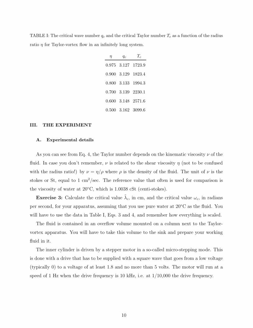
TABLE I: The critical wave number qc and the critical Taylor number Tc as a function of the radius

ratio η for Taylor-vortex flow in an infinitely long system.

η qc Tc

0.975 3.127 1723.9

0.900 3.129 1823.4

0.800 3.133 1994.3

0.700 3.139 2230.1

0.600 3.148 2571.6

0.500 3.162 3099.6

III. THE EXPERIMENT

A. Experimental details

As you can see from Eq. 4, the Taylor number depends on the kinematic viscosity ν of the

fluid. In case you don’t remember, ν is related to the shear viscosity η (not to be confused

with the radius ratio!) by ν = η/ρ where ρ is the density of the fluid. The unit of ν is the

stokes or St, equal to 1 cm2/sec. The reference value that often is used for comparison is

the viscosity of water at 20◦C, which is 1.0038 cSt (centi-stokes).

Exercise 3: Calculate the critical value λc, in cm, and the critical value ωc, in radians

per second, for your apparatus, assuming that you use pure water at 20◦C as the fluid. You

will have to use the data in Table I, Eqs. 3 and 4, and remember how everything is scaled.

The fluid is contained in an overflow volume mounted on a column next to the Taylor-

vortex apparatus. You will have to take this volume to the sink and prepare your working

fluid in it.

The inner cylinder is driven by a stepper motor in a so-called micro-stepping mode. This

is done with a drive that has to be supplied with a square wave that goes from a low voltage

(typically 0) to a voltage of at least 1.8 and no more than 5 volts. The motor will run at a

speed of 1 Hz when the drive frequency is 10 kHz, i.e. at 1/10,000 the drive frequency.

10

B. Onset of Taylor vortices

Well, it looks like we are about ready to see whether all that theory is really correct. So

let us prepare the apparatus. Drain whatever liquid may be in it into the overflow volume.

You will have to take this volume to the sink and discard the old fluid. After rinsing it, fill

the overflow volume with some de-ionized (DI) water and use this to flush out the apparatus

a time or two. Who knows what was last in there, and we do not want our fluid to be

contaminated! Now prepare one liter of DI water and 20 cc of Kalliroscope concentrate (i.e

a 2% mixture) in a beaker. Pour it into the overflow volume, attach to the apparatus, and

fill the apparatus. Again flush it once or twice with the mixture to be sure you have a

uniform fluid in the apparatus.

You already calculated the angular speed, so you know about how fast to drive the motor

to find the onset of Taylor vortices. Start at a speed well below that. At each speed, wait

long enough to give potential vortices a chance to form. Make sure you record the lab

temperature that prevails during your experiment; viscosities are temperature dependent!

At each speed, make a note in your notebook about whether vortices formed. Pay par-

ticular attention to where they first form. The theory pertains to an imagined system of

infinite length without ends. Where would this be most likely to be a good approximation

for your real apparatus?

Exercise 4: Why does it take so long for the vortices to form even after you have

exceeded the critical angular speed?

Exercise 5: Can you explain the strong vortices that form first at the ends?

After you have determined the onset frequency and have a nice pattern of vortices in

the apparatus, count how many there are. Also measure the distance between the ends of

the liquid column (between the white teflon rings) and calculate the wave number of the

vortices. How does this compare with the theory?

Now reverse the process and reduce the cylinder speed in small steps. You will have to

be patient at each step to be sure whether stable vortices still exist. Does the onset you

found going in this direction agree with what you found going up?

11

C. Eckhaus Boundary

Once you have established a nice vortex pattern above but close to onset, count the vortex

pairs and then increase the speed suddenly to twice the onset speed, i.e. to ǫ ≃ 1. Do the

vortices survive this harsh treatment?

Now turn off the motor and let the vortices decay completely. Then go again suddenly

to ǫ ≃ 1. Watch the vortices grow and describe what you see. When everything settles

down to a time independent pattern, count the vortices and calculate their wave number.

Now reduce ǫ to about 0.2. Let the pattern equilibrate. Do you still have the same wave

number? Continue to reduce ǫ in small steps and each time wait long enough to convince

yourself that you have a stable pattern. What do you find?

In the above experiment you should have observed that the pattern with the wave number

you generated by the sudden start experiment becomes unstable as you approach onset from

above. A pair of vortices will be lost after one of your small steps.

Question: Where are the vortices lost? In the interior or at the ends?

This vortex-pair loss is due to the famous Eckhaus instability that occurs in many pattern-

forming systems. Hopefully you did the above experiment slowly enough so that you lost

only a single vortex pair. You will have to let the system equilibrate for some time to get

a reasonably uniform wave number throughout; where you lost the pair the wave number

initially will be too small. Then reduce the speed further to see whether you can find

additional transitions. For each number of vortices in your system you can calculate a wave

number at which the Eckhaus instability occurs. Make a graph of this in your notebook.

How do your results compare with what you can find in the literature?

D. Secondary Bifurcations

When the speed of the inner cylinder gets large enough, the Taylor vortices become

unstable to a time-periodic mode. Waves form on each vortex and travel azimuthally. A

bifurcation to a time periodic state is called a Hopf bifurcation. Let us see whether we can

find it.

Increase the speed to about two or three times critical and let the system equilibrate.

If nothing happens, go up further in fairly large steps. Once you find this so-called wavy

12

mode, back off and see the minimum speed at which it survives. When it is gone, increase

the speed in smaller steps and get a good value for ǫw at the onset.

Now that you have this wavy state, try to determine some of its properties. How many

wave lengths are there around the circumference? What is the wavy-mode speed relative to

the inner-cylinder speed?

E. Viscosity measurements

When you are done, drain the fluid from the apparatus into your overflow volume. Fill

the viscometer with a small amount of the fluid and determine the viscosity. Did the 2%

Kalliroscope that you added to the water alter the viscosity significantly? If the viscosity

differs from what you used when you calculated ωc, re-do the calculation and see whether it

improved the agreement of your measurement with theory or whether it makes it worse.

F. Dependence on Viscosity

It would be nice to know whether the theory is right about the viscosity dependence of

the onset. So let us change ν and do the above experiment again. For this, use a mixture

of 50% water and 50% glycerol. Here too add about 20 cc of Kalliroscope concentrate to

one liter of the mixture. Do make an estimate of the onset frequency before you start the

experiment. You will need to know the viscosity of the mixture. So you better measure it.

Discuss the agreement or disagreement of your results with the theory. Don’t forget to see

also how the wave number compares with what you found before and with theory.

IV. APPENDIX: THE EQUATIONS OF MOTION

A. Number of independent variables

Since we are going to use a fluid mechanical systems to investigate various bifurcation

and pattern-formation problems, it seems appropriate to understand first the origin of the

equations of motion for fluid flow. These equations are derivable from the conservation laws

of Newtonian mechanics.

13

For a single-component system in thermodynamic equilibrium there are three extensive or

intensive variables and one relation between them [e.g. the entropy, volume, and number of

moles S, V, N , and the energy U(S, V, N), or their conjugates and the appropriate Legendre

transform of U ]. Thus, there are only two independently specifiable variables needed to

determine the state of the system. In fluid mechanics it is often convenient to use the

pressure P and the density ρ.

A flowing fluid is obviously not an equilibrium state. Nontheless, it is considered to be

an excellent approximation to assume that it is locally in equilibrium. However, the two

thermodynamic variables are now functions of the position ~r and of the time. If the fluid is

in motion, it is necessary to specify also the velocity ~v in addition to the two thermodynamic

variables. The velocity generally has three components, which may also be functions of ~r

and t. Thus, ~v = ~v(~r, t), or

~v(x, y, z, t) = u(x, y, z, t)i + v(x, y, z, t)j + w(x, y, z, t)k

where i, j, and k are the unit vectors in the x, y, and z directions. Specifying the five scalar

variables P , ρ, u, v, and w, all as a function of x, y, z, and t, completely describes the state

of the system. Thus, we need five scalar equations to completely describe the fluid flow.

B. Equations of Motion.

Since there are five independent variables, we need five equations which relate them to

each other. One of them is the equation of continuity which corresponds to mass conser-

vation. The next three can best be written as a single vector equation corresponding to

Newton’s Second Law. For a so-called ideal fluid, in which there is no dissipation due to

viscosity or thermal conduction, this equation is known as Euler’s equation. When dissi-

pation is taken into consideration, as it must be for real fluids in most cases of interest

to us, then this equation becomes the Navier-Stokes equation. The fifth equation is one

which assures entropy or energy conservation. It will not be important to our particular

case of Taylor-vortex flow because our experiments are done at constant temperature. But

for completeness, we derive it below as well.

14

1. The continuity equation.

The velocity ~v(x, y, z, t) is the velocity of the fluid at a particular point fixed in the

laboratory reference frame. Thus, ~v does not represent the velocity of a particular small

volume element of the fluid as it moves along. Rather it refers to the velocity of that fluid

material which happens to be present at a particular location at a particular time, and this

fluid material may be changing with time. Similarly, P and ρ refer to a particular point in

space.

Let us consider some macroscopic volume V0 which is fixed in space. The total mass in

this volume is

M =∫

ρdV (10)

where the integral is over the entire volume V0. The mass contained in V0 may change with

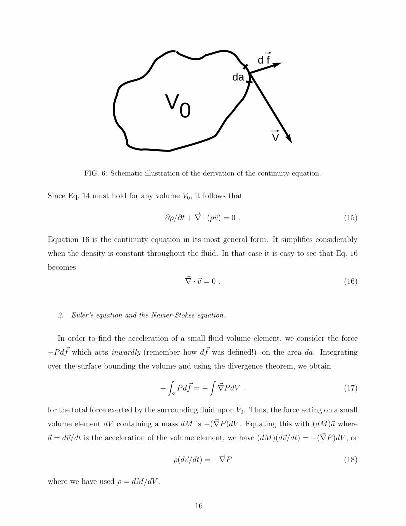
time because fluid is flowing into and out of V0. Through a small element da of the surface

which bounds V0, there is a mass flux out of V0 given by

dm = ρ~v · d~f (11)

where d~f = nda, and where n is the unit vector normal to the surface element da and

pointing in the outward direction (see Fig. 6). This is easily seen as follows. The dot-

product ~v · dn gives the velocity component in the direction of the normal, and multiplying

it by da yields the volume flow-rate out of V0 through da. Multiplying further by ρ leads to

the corresponding mass flow rate dm. Note that dm is by convention taken to be positive

when the flow is out of V0. The total mass flux out of V0 is given by the integral of dm over

the surface bounding V0, that is by∫S ρ~v · d~f . Using the divergence theorem, this can be

written as the volume integral :

∫S

ρ~v · d~f =∫

~∇ · (ρ~v)dV . (12)

But with Eq. 10, the total mass flux out of V0 is also given by ∂M/∂t = −(∂/∂t)∫

ρdV with

this last integral also over the entire volume V0. Thus we have

(∂/∂t)∫

ρdV = −

∫~∇ · (ρ~v)dV . (13)

Rearranging, one has ∫[∂ρ/∂t + ~∇ · (ρ~v)]dV = 0 . (14)

15

V0

da

d f

V

FIG. 6: Schematic illustration of the derivation of the continuity equation.

Since Eq. 14 must hold for any volume V0, it follows that

∂ρ/∂t + ~∇ · (ρ~v) = 0 . (15)

Equation 16 is the continuity equation in its most general form. It simplifies considerably

when the density is constant throughout the fluid. In that case it is easy to see that Eq. 16

becomes

~∇ · ~v = 0 . (16)

2. Euler’s equation and the Navier-Stokes equation.

In order to find the acceleration of a small fluid volume element, we consider the force

−Pd~f which acts inwardly (remember how d~f was defined!) on the area da. Integrating

over the surface bounding the volume and using the divergence theorem, we obtain

−

∫S

Pd~f = −

∫~∇PdV . (17)

for the total force exerted by the surrounding fluid upon V0. Thus, the force acting on a small

volume element dV containing a mass dM is −(~∇P )dV . Equating this with (dM)~a where

~a = d~v/dt is the acceleration of the volume element, we have (dM)(d~v/dt) = −(~∇P )dV , or

ρ(d~v/dt) = −~∇P (18)

where we have used ρ = dM/dV .

16

It is crucial to recognize that the derivative on the lhs of Eq. 18 is the total derivative of

~v. Thus, it does not represent the change in ~v with respect to t at a fixed location. Rather,

in order to conform to Newton’s Second Law, it represents the acceleration of a particular

element of fluid material and thus corresponds to the change of ~v in a frame moving along

with this particular fluid element. Therefore, in Cartesian coordinates for instance,

d~v = (∂~v/∂t)dt + (∂~v/∂x)dx + (∂~v/∂y)dy + (∂~v/∂z)dz (19)

or

d~v = (∂~v/∂t)dt + (d~r · ~∇)~v . (20)

With d~r/dt = ~v this gives

d~v/dt = ∂~v/∂t + (~v · ~∇)~v . (21)

Substituting into Eq. 18, one has

∂~v/∂t + (~v · ~∇)~v = −(1/ρ)~∇P . (22)

Equation 22 is Euler’s equation, and represents Newton’s Second Law (or linear momentum

conservation) for the ideal fluid in which there is no dissipation and no external force. If

the fluid is subjected to the gravitational field, there is an external force equal to ρ~g which

must be taken into account, yielding

∂~v/∂t + (~v · ~∇)~v = −(1/ρ)~∇P + ~g. (23)

The second term on the lhs of Eq. 22 or 23 is nonlinear in ~v. It makes it impossible to

solve the equations of motion under most circumstances in a straight forward manner, and

is responsible for most of the phenomena which occur in fluid flow and which interest us

here.

For real fluids, it is necessary to consider dissipation which was neglected in Euler’s

equation. We will not do that in detail here, but it can be accomplished by considering the

momentum flux ∂(ρ~v)/∂t. As derived from Euler’s equation, this flux is associated entirely

with reversible processes. If there is irreversibility due to viscosity, the corresponding term

can be subtracted. For an incompressible fluid in the gravitational field, this procedure leads

to[5]

∂~v/∂t + (~v · ~∇)~v = −(1/ρ)~∇P + (η/ρ)∆~v + ~g . (24)

17

Here ∆ is the three-dimensional Laplace operator [(∂2/∂x2 + ∂2/∂y2 + ∂2/∂z2) in Cartesian

coordinates], and η is the shear viscosity (in the case of compressible fluids where the density

may vary, there is an additional contribution involving the bulk viscosity ζ ; but we will have

no need to consider this dissipative mechanism). Equation 24 is the Navier-Stokes equation

for an incompressible fluid, and for us it will serve as the equation of motion appropriate for

real fluids in the presence of gravity.

When we want to consider a fluid in the presence of temperature gradients, it is convenient

to transform Eq. 24 as follows. We write the temperature T (x, y, z, t) as

T (x, y, z, t) = T0 + T1(x, y, z, t) (25)

where T0 is a constant mean temperature. Smilarly, we write the density as

ρ = ρ0 + ρ1 (26)

and the pressure as

P = P0 + P1 . (27)

For ρ0 we take the constant density corresponding to T0 and the equation of state. For small

T1/T0 we then have

ρ1 = −ρ0βT1 (28)

where β is the isobaric thermal expansion coefficient −(1/ρ)(∂ρ/∂T )p. ForP0 we take the

pressure corresponding to mechanical equilibrium when T = T0 and ρ = ρ0. It is given by

Eq. 23, and in the presence of gravity will vary with height according to

P0 = ρ0~g · ~r + constant . (29)

To lowest order in ρ1, T1, and P1 the pressure term in Eq. 24 can now be written as

~∇P/ρ = ~∇P0/ρ0 + ~∇P1/ρ0 − (~∇P0/ρ2

0)ρ1 (30)

or

~∇P/ρ = ~g + ~∇P1/ρ0 + ~gT1β . (31)

With this, the Navier-Stokes equation, Eq. 24, becomes

∂~v/∂t + (~v · ~∇)~v = −(1/ρ0)~∇P1 + ν∆~v − βT1~g (32)

where we have introduced the kinematic viscosity

ν = η/ρ . (33)

18

3. The equation of continuity of the entropy or the energy.

In an ideal fluid there cannot be any heat transport from one part to another, and the

entropy per unit mass s of any fluid particle remains constant at all times; i.e. ds/dt = 0.

By arguments similar to those used to derive the continuity equation Eq. 16, one has

∂(ρs)/∂t + ~∇ · (ρs~v) = 0 . (34)

If by virtue of the initial conditions s is uniform throughout the fluid, it will remain uniform

at all times. Then the motion is isentropic and Eq. 34 becomes s = constant. Equations 16,

32, and 34 give the five scalar equations which determine the motion of the ideal fluid.

Alternatively to Eq. 34, we could have focused on an equation for the energy flux. We

would again start with the ideal fluid, and consider some volume V0. We equate the time rate

of change of the energy in this volume with the flux across the surface bounding the volume.

The total energy in V0 can be written as a sum of the kinetic and the internal energy, and

its time rate of change is given by (∂/∂t)∫(ρv2/2 + ρǫ)dV , where ǫ is the internal energy

per unit mass. Equating with the flux across the surface, we get

(∂/∂t)∫

(ρv2/2 + ρǫ)dV = −

∫S

ρ(v2/2 + ǫ + P/ρ)~v · d~f . (35)

On the rhs, the contribution P/ρ corresponds to the work done by pressure forces on the

volume V0. Using the divergence theorem, this gives

(∂/∂t)∫

(ρv2/2 + ρǫ)dV = −

∫~∇ · ρ(v2/2 + ǫ + P/ρ)~vdV . (36)

Since Eq. 36 must hold for any V0, we have

(∂/∂t)(ρv2/2 + ρǫ) = −~∇ · ρ(v2/2 + ǫ + P/ρ)~v . (37)

Equations 34 and 37 should not be thought of as independent of each other. Indeed, one

can be derived from the other because the energy and entropy are not independent thermo-

dynamic variables. Thus there remain only five relationships between the five scalar fields

of hydrodynamics.

Equations 34 and 37 contain only the reversible fluxes. When the fluid is not ideal, they

must be modified by including dissipative terms. For our purposes, the most important

contribution will come from the conduction of heat when the temperature is not uniform.

19

In that case, there is a heat-flux density ~q which can be expanded in a power series of

the temperature gradient ~∇T . Since ~q vanishes when ~∇T is zero, the lowest term in the

expansion gives

~q = −λ~∇T . (38)

The coefficient λ is called the thermal conductivity of the fluid. Since heat flows from high

to low temperatures, the minus sign in the equation implies that λ > 0. We can now include

the dissipative flux due to thermal conduction in the entropy- and energy-flux equations,

Eqs. 34 and 37. We obtain

ρT (∂s/∂t + ~v · ~∇s) = ~∇ · (λ~∇T ) (39)

and

(∂/∂t)((1/2)ρv2 + ρǫ) = −~∇ · [ρ((1/2)v2 + ǫ + P/ρ)~v − λ~∇T ] (40)

respectively. In principle, viscous dissipative terms should be included in Eqs. 39 and 40 as

well; but in practice for our applications the viscosity makes a major contribution only in

the Navier-Stokes equation, Eq. 32, and we will neglect these terms in the energy or entropy

equation.

It is often convenient to write the entropy-flux equation in terms of the temperature T . If

the pressure variations in the fluid are so small that the corresponding changes in density can

be neglected (which is the case when the velocity is much less than the velocity of sound),

then T ~∇s = cp~∇T , and Eq. 39 yields

ρcp(∂T/∂t + ~v · ~∇T ) = ~∇ · (λ~∇T ) . (41)

If we further assume that temperature variations are so small that λ may be regarded as

constant, then

∂T/∂t + ~v · ~∇T = κ∆T . (42)

where

κ = λ/ρcp (43)

is the thermal diffusivity. In real incompressible fluids with a nonuniform temperature,

Eq. 42 together with the Navier-Stokes equation Eq. 32 and the continuity equation Eq. 16

provide an excellent approximation to the five relations which determine the fluid flow.

20

C. Boundary conditions.

In Sect. IVB we discussed the equations of motion of fluid flow. A particular fluid-flow

problem is not defined, however, until boundary conditions (BC) have been specified. Usu-

ally there are solid walls which define the geometry of the fluid and which are impermeable.

There may also be conditions imposed upon the temperature or upon the temperature gra-

dient at the walls. For an ideal fluid, we generally have vn = 0 at any stationary solid wall.

Here vn is the component of ~v normal to the wall. This is so because there is no flow into or

out of the wall. This BC by itself, without any constraint on the velocity components tan-

gential to the wall, often is called a ”free” BC because the fluid is free to move tangentially.

In a real fluid, the components of ~v tangential to a stationary wall also vanish because the

viscosity assures that any fluid immediately adjacent to the wall is stationary. This BC often

is referred to as a ”rigid” BC. If the wall is moving, then for rigid BC’s the fluid will move

with it. Thus, for real fluids adjacent to a wall ~v = ~vw, where ~vw is the wall velocity. For an

incompressible fluid the condition that the velocity component tangential to the wall must

vanish implies that the gradient of the velocity component perpendicular to the wall van-

ishes also. This is easy to see as follows. Let the z-component w of ~v be normal to the wall,

with the x and y components u and v tangential to the wall. Then (∂u/∂x) = (∂v/∂y) = 0

because u and v vanish for all x and y. In that case, by virtue of Eq. 16 (∂w/∂z) must

vanish also. That is, both the velocity and its gradient vanish at a rigid wall. Ideal-fluid

(i.e. free) boundary conditions are often used because they greatly simplify the solution of

many problems without loosing the qualitative physics of the fluid flow. Although often the

real fluid-flow problem differs from the ideal one only in quantitative aspects, there are cases

where there is a qualitative difference.

D. Circular Couette flow.

As an example of a fluid-flow problem, let us consider an idealized version of the system

described in Sect. II, and in particular by Fig. 4. It has a uniform temperature, i.e. T1 = 0.

Therefore Eq. 42 is trivially satisfied, and the last term on the rhs of Eq. 32 is zero. The

system consists of two concentric cylinders rotating about their axis. We take this axis in

the x-direction. Here we will take these cylinders to be infinitely long so as to avoid the

21

complications associated with the boundaries in the axial direction. The inner cylinder,

of radius r1, rotates with angular speed ω1, and the outer one, of radius r2, with angular

speed ω2. In most of the examples we will consider later on, ω1 = ω and ω2 = 0, i.e. the

outer cylinder is stationary. It is convenient to make the variables dimensionless. Although

there are several ways of doing this, a particularly good one is to measure length, time, and

velocity in units of d = r2 − r1, d2/ν , and ω1r respectively. Equation 32 then becomes

∂~v/∂t + Ri(~v · ~∇)~v = −~∇P + ∆~v . (44)

This equation contains only one independently variable parameter, namely the Reynolds

number of the inner cylinder

Ri = ω1r1d/ν . (45)

However, two other parameters are hidden away in the BC’c. One of them is the outer

cylinder speed, which can be written as a second Reynolds number

R2 = ω2r2d/ν . (46)

The third is the ratio

η = r1/r2 (47)

of the two cylinder radii. All Couette-Taylor systems with the same R1, R2, and η will

behave in the same way, regardless of the detailed values of d, ν, ω1, and ω2. For the physical

system there is of course one additional parameter, namely the axial length of the apparatus.

The boundary conditions are most easily imposed after re-writing Eq. 44 in cylindrical

coordinates (r, φ, x) (which we will not do explicitly here). The symmetry of the boundaries

suggests that there should be a time independent solution for which the components of

~v(r, φ, x) are

vx = vr = 0 , (48)

vφ = vφ(r) , (49)

and

P = P (r) . (50)

A more careful analysis confirms this, and one obtains the two ordinary differential equations

dP/dr = ρv2

φ/r (51)

22

and

d2vφ/dr2 + (1/r)(dvφ/dr) − vφ/r2 = 0 . (52)

It is worth noting that the problem is so easy because the nonlinear term in the Navier-

Stokes equation vanishes identically. This is so because, as implied by Eq. 26, ~v has a

non-vanishing component only in the φ-direction, whereas the gradient of ~v is entirely in the

r-direction. Thus the term (~v · ~∇)~v vanishes and we are left with a linear partial differential

equation which trivially separates into ode’s. This orthogonality between ~v and its gradient

is a general property of shear flows.

Equation 52 has a solution of the form

vφ = ar + b/r . (53)

The constants a and b are determined by the boundary conditions. For rigid BC’s we have

vφ = r1ω1 for r = r1 and vφ = r2ω2 at r = r2. This yields

a = (ω2r2

2− ω1r

2

1)/(r2

2− r2

1) (54)

and

b = (ω1 − ω2)r2

1r2

2/(r2

2− r2

1) . (55)

The pressure can be found by integrating Eq. 51 after substituting the results for vphi.

Although we have found a solution of the Navier-Stokes equation for the circular Couette

boundary conditions, we have not yet established that this solution is stable. It turns out

that Couette flow is stable for small ω1, but gives way to more complicated patterns such

as Taylor-vortex flow for larger ω1.

E. Stability of fluid flow.

Let us assume that we have found a solution ~v0 to the equations of motion for a particular

fluid-flow problem, such as the circular Couette state in the Couette-Taylor system given

by Eqs. 7 to 9. We still have no assurance that these solutions are stable. By this we mean

that there might be some disturbances which, if imposed upon the flow, would grow and

would cause the system to choose another flow state. Here we only give a general outline

of how to test for stability. To actually carry out the procedure usually involves numerical

calculations [4] and its complexity is beyond the scope of our work.

23

We write the velocity, temperature, and pressure fields as

~v = ~v0 + ~v1, III.34a

T = T0 + T1, III.34b

and

P = P0 + P1. III.34c

Here we regard ~v1, T1, and P1 as a small perturbations of the solution ~v0, T0, and P0. Substi-

tuting into Eqs. 8, 23, and 14a, 14b, or 14c, the terms involving only ~v0, T0, and P0 cancel

because these functions satisfy the equations. There remains an equation for ~v1, T1, and

P1 which may contain the known functions ~v0, T0, and P0 as coefficients. Since ~v1, T1, and

P1 are considered small perturbations, we can omit nonlinear terms such as ~v1 ·~∇~v1, and

obtain, for instance from the Navier-Stokes and continuity equations,

∂~v1/∂t + (~v0 ·~∇)~v1 + (~v1 ·

~∇)~v0 = −~∇P1/ρ + ν∆~v1 III.35

and

~∇ · ~v1 = 0. III.36

In the RB case, the disturbance of T must also be substituted in Eq. 31c. If we write the

disturbance ~v1 as

~v1 = A(t)~f(x, y, z), III.37

and take A to have the form

A(t) = constant × exp(γt)exp(−iωt) III.38

then we can determine whether the growth rate γ is positive or negative. The original

solution ~v0 is stable only if the growth rates are negative for all ~f(x, y, z). Of course to

determine the nature of the solution corresponding to a growing ~v1 requires the solution of

nonlinear equations; and generally this is a difficult problem.

[1] A sizable literature now exists dealing with this system. A comprehensive review has been

given by R.C. DiPrima and H.L. Swinney, in Hydrodynamic Instabilities and Transitions to

24

Turbulence, edited by H.L. Swinney and J.P. Gollub (Springer, Berlin, 1981). Important early

papers in this field are numerous; but particularly noteworthy are D. Coles, J. Fluid Mech. 21,

385 (1965); and H.A. Snyder, J. Fluid Mech. 35, 273 (1969); and J.E. Burkhalter and E.L.

Koschmieder, Phys. Fluids 17, 1929 (1974).

[2] G.I. Taylor, Philos. Trans. Roy. Soc. London Ser. A 223, 289 (1923).

[3] M.A. Dominguez-Lerma, D.S. Cannell, and G. Ahlers, Phys. Rev. A 34, 4956 (1986).

[4] M.A. Dominguez-Lerma, G. Ahlers, and D.S. Cannell, Phys. Fluids 27, 856 (1984).

[5] L.D. Landau and E.M. Lifshitz, Fluid Mechanics (Pergamon, London, 1959).

25