Pattern Discovery for Hypothesis Generation in … · Pattern Discovery for Hypothesis Generation...
182
Pattern Discovery for Hypothesis Generation in Biology by Aristotelis Tsirigos A dissertation submitted in partial fulfillment of the requirements for the degree of Doctor of Philosophy Department of Computer Science New York University January, 2006 _______________________ Dennis Shasha _______________________ Isidore Rigoutsos
-
Upload
dangkhuong -
Category
Documents
-
view
222 -
download
0
Transcript of Pattern Discovery for Hypothesis Generation in … · Pattern Discovery for Hypothesis Generation...
Pattern Discovery for Hypothesis
Generation in Biology
by
Aristotelis Tsirigos
A dissertation submitted in partial fulfillment
of the requirements for the degree of
Doctor of Philosophy
Department of Computer Science
New York University
January, 2006
_______________________
Dennis Shasha
_______________________
Isidore Rigoutsos

© Aristotelis Tsirigos
All Rights Reserved, 2006

iii
DEDICATION
This dissertation is dedicated to my family in Greece.

iv
ACKNOWLEDGEMENTS
First and foremost I would like to thank my advisor Dennis Shasha for his
guidance and patience during these four years. He trusted me with
important research projects while allowing me at the same time to take
Spanish classes and do part of my research at IBM. My co-advisor at
IBM Research Isidore Rigoutsos provided me with an excellent research
environment at IBM Research both in terms of interesting computational
problems and in terms of research collaborators inside and outside IBM.
Ken Birnbaum’s lab at New York University and Philip Benfey’s lab at
Duke University have been instrumental in our efforts to improve and
validate our computational techniques. I would like to also thank the
computer science professors and committee members Dan Melamed
and Mehryar Mohri for extremely helpful discussions on machine
learning techniques and their applications. I would especially like to
thank NYU biology professors Fabio Piano and Kris Gunsalus for
introducing me to the basic concepts and mechanisms in biology during
my first years at NYU. My IBM collaborators Kevin Miranda, Alice

v
McHardy, Tien Huynh, Laxmi Parida and Dan Platt helped make
research at IBM fun and productive. I would also like to acknowledge the
enormous support I received from Computer Science department
administration in dealing with the necessary bureaucracy regarding my
employment by IBM Research as a graduate co-op. More specifically, I
would like to thank the director of graduate studies professor Denis
Zorin, the department chair Margaret Wright, as well as Rosemary
Amico, Anina Karmen, Maria Petagna, Daphney Boutin and Lourdes
Santana. Finally, I would like to thank our graduate assistant union
GSOC for guaranteeing decent salaries, benefits and working conditions
for all graduate students at NYU and for promoting a sense of solidarity
among its members.
vi
ABSTRACT
In recent years, the increase in the amounts of available genomic as well
as gene expression data has provided researchers with the necessary
information to train and test various models of gene origin, evolution,
function and regulation. In this thesis, we present novel solutions to key
problems in computational biology that deal with nucleotide sequences
(horizontal gene transfer detection), amino-acid sequences (protein sub-
cellular localization prediction), and gene expression data (transcription
factor - binding site pair discovery). Different pattern discovery
techniques are utilized, such as maximal sequence motif discovery and
maximal itemset discovery, and combined with support vector machines
in order to achieve significant improvements against previously proposed
methods.

vii
DEDICATION____________________________________ iii
ACKNOWLEDGEMENTS __________________________ iv
ABSTRACT _____________________________________ vi
List of Figures ___________________________________ x
List of Tables __________________________________ xiv
1 Introduction ___________________________________ 1
2 Machine learning methods in bioinformatics ________ 3
2.1 Unsupervised pattern discovery _______________________ 3
2.2 Probabilistic models_________________________________ 7
2.2.1 Bayesian Networks _____________________________________7
2.2.2 Probabilistic Relational Models ___________________________10
2.3 Distribution-free methods ___________________________ 12
2.3.1 Boosting_____________________________________________13
2.3.2 Support Vector Machines _______________________________15
3 Horizontal Gene Transfer _______________________ 19
3.1 Related work ______________________________________ 20
viii
3.2 Generalized compositional features ___________________ 31
3.2.1 From compositional features to gene typicality scores _________33
3.2.2 Our proposed algorithm, Wn, for HGT detection: individual genes 36
3.2.3 Our proposed algorithm, Wn, for HGT detection: clusters of
transferred genes ____________________________________________38
3.2.4 Our proposed algorithm, Wn, for HGT detection: automated
threshold selection ___________________________________________39
3.2.5 Results______________________________________________40
3.2.5.1 Case 1: donor pool comprising phage genes _______________ 41
3.2.5.2 Case 2: donor pool comprising genes from archaeal and bacterial
genomes. ____________________________________________________ 47
3.2.6 Discussion ___________________________________________50
3.3 A New Similarity Measure: one-class SVM______________ 54
3.3.1 Results______________________________________________58
3.3.1.1 Evaluation of Wn-SVM: prokaryotic donor and prokaryotic hosts 59
3.3.1.2 Evaluation of Wn-SVM: analysis of the human cytomegalovirus
genome______________________________________________________ 63
3.3.2 Conclusion___________________________________________66
4 Protein Localization ___________________________ 87
4.1 Related work ______________________________________ 88
4.2 Overview of unsupervised pattern discovery ___________ 90

ix
4.3 Method A: fixed-length patterns ______________________ 92
4.4 Method B: variable-length patterns____________________ 95
4.5 Results___________________________________________ 98
4.5.1 Method A: fixed-length patterns __________________________98
4.5.2 Method B: variable-length patterns _______________________102
4.5.3 Hybrid Method B/A: fixed- and variable-length patterns _______102
4.6 Conclusion ______________________________________ 104
5 Transcription factor binding site prediction_______ 115
5.1 Related work _____________________________________ 116
5.2 Methods_________________________________________ 121
5.2.1 Discovering bi-clusters ________________________________121
5.2.2 The proposed model __________________________________125
5.3 Results__________________________________________ 131
5.3.1 Dataset ____________________________________________131
5.3.2 Testing_____________________________________________132
6 Future work _________________________________ 143
Bibliography___________________________________ 144
x
List of Figures
Figure 1: Example of a template............................................................ 75
Figure 2: Demonstrating the automatic method for selecting a score
threshold using the genome of Aeropyrum pernix as a test case (see
also text)......................................................................................... 76
Figure 3: Overall performance m
Perf of five scoring methods that has
been averaged over 123 genomes: (a) case of a phage donor gene
pool, (b) case of a prokaryote donor gene pool. ............................. 77
Figure 4: Achieved relative improvement of W8 vs. CAI averaged over all
experiments and all genomes (see also text). ................................ 78
Figure 5: Average relative improvement CAI
GRel of W8 over CAI for each
one of 123 organisms. Each point is an average over 100
experiments with donor genes drawn from the phage gene pool (see
also text)......................................................................................... 79
Figure 6: Average relative improvement CAI
GRel of W8 over CAI for each
one of 123 organisms. Each point is an average over 1000
xi
experiments with donor genes drawn from the prokaryote gene pool
(see also text)................................................................................. 80
Figure 7: Achieved overall performance mPerf as a function of template
size and for different percentages of artificially added genes: (a)
case of phage gene donor pool, (b) case of prokaryotic gene donor
pool. ............................................................................................... 81
Figure 8: Detecting the vancomycin-resistance cluster of horizontally
transferred genes in Enterococcus faecalis. In an ideal setting, the
genes of this cluster should be reported as a group (i.e. their ranks
for a given scoring scheme should be as close to each other as
possible) and uninterrupted by genes that do not belong to the
cluster. Additionally, the ideal method should be able to report
typicality scores for the group as a whole that are as low as
possible, or, equivalently, assign gene ranks to these genes that are
as low as possible (see also text)................................................... 82
Figure 9: Achieved relative improvement of W8-SVM vs. CAI and of W8-
SVM vs. W8. The results represent an average over all experiments
and all genomes (see also text). .................................................... 83
Figure 10: Average relative improvement W8
GRel of W8-SVM over W8 for
each one of 123 organisms. Each point is an average over 20
xii
experiments with donor genes drawn from the prokaryote gene pool
(see also text)................................................................................. 84
Figure 11: Average relative improvement CAI
GRel of W8-SVM over CAI for
each one of 123 organisms. Each point is an average over 20
experiments with donor genes drawn from the prokaryotic gene pool
(see also text)................................................................................. 85
Figure 12: Horizontal transferred regions in the HHV5 genome, strain
AD169. ........................................................................................... 86
Figure 13: Training/testing for method based on fixed-length pattern
discovery (Method A). .................................................................. 106
Figure 14: Training/testing for method based on variable-length pattern
discovery (Method B). .................................................................. 107
Figure 15: 5-fold cross-validation for Method A. .................................. 108
Figure 16: Tradeoff between accuracy and coverage using Method B as
standalone.................................................................................... 109
Figure 17: 5-fold cross-validation for hybrid Method B/A..................... 110
Figure 18: Comparison of our method with PLOC............................... 111
Figure 19: A transcription factor expression profile (red) plotted against
three gene expression profiles in several experimental conditions.
..................................................................................................... 133
xiii
Figure 20: Scatter plot of gene expression and transcription factor
expression profiles. ...................................................................... 134
Figure 21: Links between a transcription factor and a potential binding
site can be constructed using gene expression and gene upstream
sequence information. .................................................................. 135
Figure 22: Model 1 – begin with a cis element, compute its aggregate
expression and correlate with transcription factor expression. ..... 136
Figure 23: Model 2 - begin with a transcription factor, find a set of highly-
correlated genes and look at their upstream regions for over-
represented cis elements. ............................................................ 137
Figure 24: Proposed model – find the gene set where all genes are
highly correlated to a transcription factor and contain the potential
binding site in their upstream regions, and then discover all bi-
clusters in that set. ....................................................................... 138
Figure 25: (a) simple interaction model between a transcription factor
and its downstream genes, (b) realistic model includes genes
upstream of the transcription factor and downstream of the regulated
genes. .......................................................................................... 139
Figure 26: Comparison against simple correlation .............................. 140
xiv
List of Tables
Table 1: List of phages .......................................................................... 71
Table 2: Gene scoring methods ............................................................ 72
Table 3: Overall performance mPerf for the methods under evaluation. 72
Table 4: Improvement of reported W8 method over previous methods. 73
Table 5: Gene scoring methods ............................................................ 73
Table 6: Overall performance mPerf for the methods under evaluation
(higher numbers are better – see also text for a definition of mPerf ).
....................................................................................................... 74
Table 7: Improvement of the new W8-SVM method over CAI and over
W8.................................................................................................. 74
Table 8: Chemical equivalence classes for amino acids. .................... 112
Table 9: Examples of patterns............................................................. 113
Table 10: Comparison of prediction accuracy (sensitivity) for the 12 sub-
cellular locations. The PLOC data is taken from [106].................. 114
Table 11: List of transcription factors with their experimentally validated
binding sites. ................................................................................ 141

xv
Table 12: Nucleotide codes. ................................................................ 142

1
1 Introduction
There is an enormous variety in the kind of data involved in
biology and their mathematical representations can range from the
simplest, e.g. scalar values, to the most complex, e.g. graphs.
Commonly used representations are listed below:
• vectors (gene expression, features)
• sequences (DNA, RNA, protein sequences)
• sets (protein families)
• trees (phylogenetic trees)
• graphs (regulatory networks, pathways)
Given the complexity of biological processes, and therefore the
complexity of the mathematical models used to describe these
processes as well as the possibility that the latter may involve any
combination of the kind of data mentioned above, both in terms of input
and in terms of output, it is obvious that rigorous probabilistic and
computational learning methods are required to combine all this diverse
data and help infer biologically meaningful predictions. In this thesis, we
2
apply pattern discovery and machine learning techniques to three distinct
problems: horizontal gene transfer detection, protein sub-cellular
localization prediction and discovery of binding site - transcription factor
pairs.
In chapter 2, we present an overview of fundamental pattern
discovery and machine learning techniques that are frequently applied to
problems in computational biology. In chapter 3, we introduce and
discuss a novel computational method for identifying horizontal transfers
using gene nucleotide composition. In chapter 4, we introduce a new
pattern-based method for the prediction of a protein’s sub-cellular
location that relies on the analysis of the corresponding amino acid
sequence. In chapter 5, we propose a novel method for the discovery of
candidate binding sites for transcription factors via the computation of bi-
clusters. Finally, in chapter 6, we conclude this thesis with some ideas
about future research.
3
2 Machine learning methods in bioinformatics
Machine learning methods for computational biology can be
divided into three categories:
• unsupervised pattern discovery
• probabilistic modeling
• large-margin learning
In the next three sections we provide a brief overview of the
relevant methods in each category.
2.1 Unsupervised pattern discovery
Pattern discovery is a research area that focuses on the
development of efficient unsupervised methods for extracting
“interesting” pieces of data given a set of objects, mainly sequences,
although active research is being done on more complex objects, such
as trees and graphs. Pattern discovery is widely used in problems where
there is minimal prior knowledge about the structure of the observed

4
sequences. This minimal knowledge is usually reflected in the
representation scheme of the sequences, which defines the alphabet of
the patterns, and gives some hints about the language that should be
used to describe them.
According to Brazma et al. 1998 [1], the pattern discovery problem
can be divided into three sub-problems:
• choosing the appropriate language to describe patterns (mismatch
patterns, regular expressions with restricted and unrestricted
number of wild cards, probabilistic modeling)
• choosing the scoring function for comparing patterns (e.g. pattern
statistical significance)
• designing an efficient algorithm that will be used to find the
patterns.
Pattern discovery methods can either be sequence driven, mostly
based on alignments, or pattern-driven, where all patterns that occur at
least k times are enumerated. Pattern-driven approaches can often be
designed to run in linear time with respect to the number of output
patterns.
The probabilistic models usually employed to describe a pattern
or, equivalently, a motif, are variations of Position-Specific Scoring
Matrices (PSSMs) obtained as a summary of multiple motif alignments.
5
Different searching methods have been used resulting in different tools:
the Gibbs Motif Sampler (Lawrence et al. 1993 [2], Neuwald et al. 1995
[3]), based on Gibbs sampling, MEME (Bailey and Elkan 1995 [4]),
based on multiple runs of the Expectation Maximization algorithm,
AlignACE (Roth et al. 1998 [5]), based on information content
maximization, PSI-BLAST (Altschul et al. 1997 [6]), based on iterative
refinement of initial sequence alignments, CONSENSUS (Hertz and
Stormo 1999 [7]), and other (Rocke and Tompa 1998 [8], Wolfertstetter
et al. 1996 [9]).
The pattern-driven tool Teiresias1, developed by the IBM
Bioinformatics Research Group, for the discovery of patterns in biological
sequences, described in Rigoutsos and Floratos (1998) [10, 11], and in
Hart et al. (2000) [12], operates in two phases: scanning and
convolution. During the scanning phase, elementary patterns with
sufficient occurrences are found, and during the convolution phase the
elementary patterns are synthesized into progressively larger patterns
until all maximal patterns are generated. A pattern is maximal if and only
if it is not subsumed by any other pattern that has the same location list,
1 Named after the famous blind prophet Teiresias in ancient Greece
6
i.e. it occurs in the same set of sequences. The running time of the
algorithm is linear with respect to the number of output patterns.
Other approaches utilize the well-known suffix tree data structure
(McCreight 1976 [13]; Ukkonen 1995 [14]). When sequences are
organized into suffix trees, any query about a pattern can be answered
by starting reading from the root of the tree without any searching and
independent of the size of the sequence. There are many bioinformatics
applications of suffix trees (Gusfield 1997 [15]). One of the pattern
discovery tools based on suffix trees is Verbumculus (Lonardi 2001 [16],
Apostolico, Bock, and Lonardi 2002 [17]).
Xlandscape (Levy et al. 1998 [18]) was designed for on-line
pattern queries and graphical analysis and visualization based on the
suffix array data structure (Manber and Myers 1990 [19]). It can also
detect repeating patterns of words, such as tandem repeats, and over-
represented words in a given database.
Vilo (2002) [20] modified the writeonly-topdown algorithm (wotd)
for constructing the suffix trees (Giegerich and Kurtz 1995 [21];
Giegerich, Kurtz, and Stoye 1999 [22]) to perform pattern discovery for
different pattern languages (mismatch patterns, regular expressions with
restricted and unrestricted number of wild cards) and in several distinct
7
settings (patterns that appear at least k times, sort patterns according to
their score, find overrepresented patterns in a sample subset).
2.2 Probabilistic models
Probabilistic models that are frequently used in biology include
Bayesian Networks (BNs) and Probabilistic Relational Models (PRMs).
We review the basic concepts below.
2.2.1 Bayesian Networks
Bayesian networks were introduced by Pearl in 1998 [23]. A
Bayesian Network (BN) is defined over a set of random variables
{ }1,..., NX X X= and provides a static model of their interdependence
both qualitatively and quantitatively.
Qualitatively, random variables are represented by nodes in a
graph G and conditional dependencies between relevant random
variables are represented by directed edges pointing from the node
representing the independent variable to the one representing the
dependent one. For any given variable Xi the set of the variables on
8
which it depends, i.e. its parents in the graphical representation, is
denoted by iPa .
Quantitatively, the probability distribution of the dependent
variable Xi is modeled as a conditional probability distribution (CPD)
( )| ;i i iP X Pa θ with respect to the parent variables in set iPa , where iθ
is the parameter vector associated with the CPD. There are several
different types of CPDs depending on whether the relevant random
variables are discrete or continuous. Widely used CPDs include tables
for discrete variables, regression trees for the case where the parent
variables are continuous and the dependent variable is discrete, softmax
(linear threshold) functions, Gaussian when all relevant variables are
continuous, and others.
Given the conditional probabilities, we can compute the joint
probability distribution using the chain rule:
( ) ( )1 1
1
,..., ; ,..., | ;N
N N i i i
i
P X X P X Paθ θ θ=
= ∏
Learning a BN model with a known structure G involves
determining the parameters 1,..., Nθ θ of the CPDs, given a training set D
which comprises multiple observations over the random variables whose
9
joint probability is modeled by the BN. The main idea is to find those
parameters that maximize the probability of the observed data given the
model:
( ) ( )1 1 1| ,..., ,..., ; ,..., N N N
X D
P D P X Xθ θ θ θ∈
= ∏
assuming that the observed data is chosen independently. The
maximization problem can be posed as:
( )( )
( )( )
( )1
1 1
* *1 1 1
,..., ,...,
,..., arg max ,..., | arg max | ,..., ( ,..., )N
N N
N N NP D P D Pθ θ θ θ
θ θ θ θ θ θ θ θ= =
Unfortunately, only in very few practical cases is it possible to find
a global maximum for the parameters sought, both because of the lack of
continuity in most CPDs used in practice, and because of some of the
random variables, the so-called hidden variables, cannot be directly
observed, and therefore they do not belong in the training set. In
practice, Expectation Maximization (EM) is used to compute an estimate
of the parameters. EM begins by randomly choosing the parameters of
the BN and it then proceeds to an iterative procedure comprising two
steps. First, given the current estimate of the parameters, the expected
statistics of the random variables on the training data are computed.
10
Then, for each CPD, and assuming that the expected statistics obtained
from the previous step are the true statistics, we re-estimate its
parameters by simply maximizing their probability. The EM procedure will
converge (under some assumptions) to a local maximum.
For more information about training Bayesian Networks and
learning their structure the reader is referred to Heckerman’s tutorial [24].
2.2.2 Probabilistic Relational Models
Although Bayesian Networks have been applied with great
success in a wide variety of applications, including in biology, the
availability of more data and, more importantly, its increasing specificity,
underline the inflexibility and, ultimately, the inadequacy of Bayesian
Networks to accurately model the complex interactions omnipresent in
the biological domain.
The limitations of Bayesian Networks stem from the fact that they
lack the concept of an “object”, and therefore they cannot account for
cases where entities modeled by several random variables (attributes)
behave in similar, but not necessarily identical, ways. Consequently,
some form of parameter sharing must be enabled. For example, in a
regulatory network comprising transcription factors and motifs, each of

11
the two classes of nodes should be allowed to share common properties
that are different for each class. Probabilistic Relational Models (PRMs)
(Koller and Pfeffer, 1998 [25], Getoor, 2001 [26]) extend Bayesian
Networks towards that direction.
An RPM schema consists of fixed BN-like parent/child
relationships embedded in a dynamic relational model, the relational
schema, comprising the following:
• A set of n classes of objects: C = {C1, … , Cn}
• For each class C, a set of attributes A(C), the random variables
that collectively describe the objects of class C
• For each class C, a set of BN-like dependencies between the
attributes of the class represented by a structure S(C)
• For each class C, a set of reference slots R(C), which mark the
dependencies of the attributes of class C on attributes of other
classes
From the description above, it is obvious that random variables
can potentially have two types of parents, depending on whether the
parent variable belongs to the same or different class.
The fact that there is a relation (reference slot) between two
classes does not mean that all objects in the two classes will be related.

12
The actual relations among the objects are represented by the relational
skeleton σ, which can be conceptualized as a graph defined on the
objects.
General algorithms developed for training the parameters of the
relational schema, as well as searching for the skeleton with the highest
likelihood, can be found in Getoor (2001) [26]. The objective is always to
maximize the a posteriori probability of the training data given the model
parameters.
2.3 Distribution-free methods
In computational learning we are generally given a set of inputs
nxx ,...,1 , randomly sampled from the input space X , together with their
corresponding outputs nyy ,...,1 in the output space Y , and the learning
task is to find a function YXf →: which maps any Xx ∈ to a
prediction )(ˆ xfy = . Distribution-free methods assume no prior model
for the data, and select a model f that minimizes the generalization
error (loss) ( )fL , i.e. the expected error when it is applied to the entire
input space:

13
( ) ( )∫∈
≠=Xx
yxfPfL )(
This is achieved by a choice of f that yields the maximum margin
on the training set, where margin is a measure of how far, under a pre-
selected distance metric, the data is from being misclassified under
model f . Boosting and Support Vector Machines are the two large-
margin training algorithms widely used in practice and we discuss them
next.
2.3.1 Boosting
The boosting algorithm [27-29] chooses a set of weights 1,..., Tw w
over T hypotheses, where T is the number of iterations of the algorithm,
so that the final hypothesis, constructed from the weighted sum of the
predictions of the individual hypotheses, minimizes a fixed loss function
over the training data { }( , ) | 1..i iS x y i N= = . Most widely used loss
functions are the exponential loss function:
( ) { }1
exp ( ) N
i i
i
L f y f x=
= −∑
14
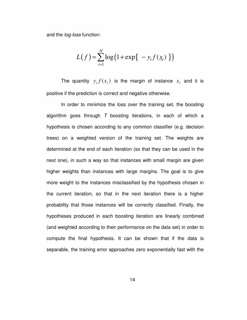
and the log-loss function:
( ) { }( )1
log 1 exp ( ) N
i i
i
L f y f x=
= + −∑
The quantity )( ii xfy is the margin of instance ix and it is
positive if the prediction is correct and negative otherwise.
In order to minimize the loss over the training set, the boosting
algorithm goes through T boosting iterations, in each of which a
hypothesis is chosen according to any common classifier (e.g. decision
trees) on a weighted version of the training set. The weights are
determined at the end of each iteration (so that they can be used in the
next one), in such a way so that instances with small margin are given
higher weights than instances with large margins. The goal is to give
more weight to the instances misclassified by the hypothesis chosen in
the current iteration, so that in the next iteration there is a higher
probability that those instances will be correctly classified. Finally, the
hypotheses produced in each boosting iteration are linearly combined
(and weighted according to their performance on the data set) in order to
compute the final hypothesis. It can be shown that if the data is
separable, the training error approaches zero exponentially fast with the
15
number of iterations, and that the final hypothesis induced by the
boosting algorithm minimizes the generalization error according to the
large-margin principle.
The initial boosting algorithm was intended to solve the binary
classification problem. However, several extensions where introduced to
perform more complex learning tasks, such as ranking [28], permutations
[30], and learning a set of constraints as a generalization of multi-class
learning [31].
2.3.2 Support Vector Machines
Support Vector Machines (SVM) [32] finds a hyperplane that
separates the positive from the negative instances in a fixed (pre-
selected) feature space )(⋅ψ for binary classification. The separating
hyperplane chosen by the original SVM algorithm is the one that
maximizes the distance (margin) from the hyperplane of those instances
closest to it. These instances are called support vectors and this is where
the name of learning algorithm originates. In practice, data is expected to
be noisy, and therefore a realistic model should also account for outliers,
i.e. instances that find themselves on the “wrong side” of the hyperplane.
In mathematical terms, the hyperplane is defined as follows:
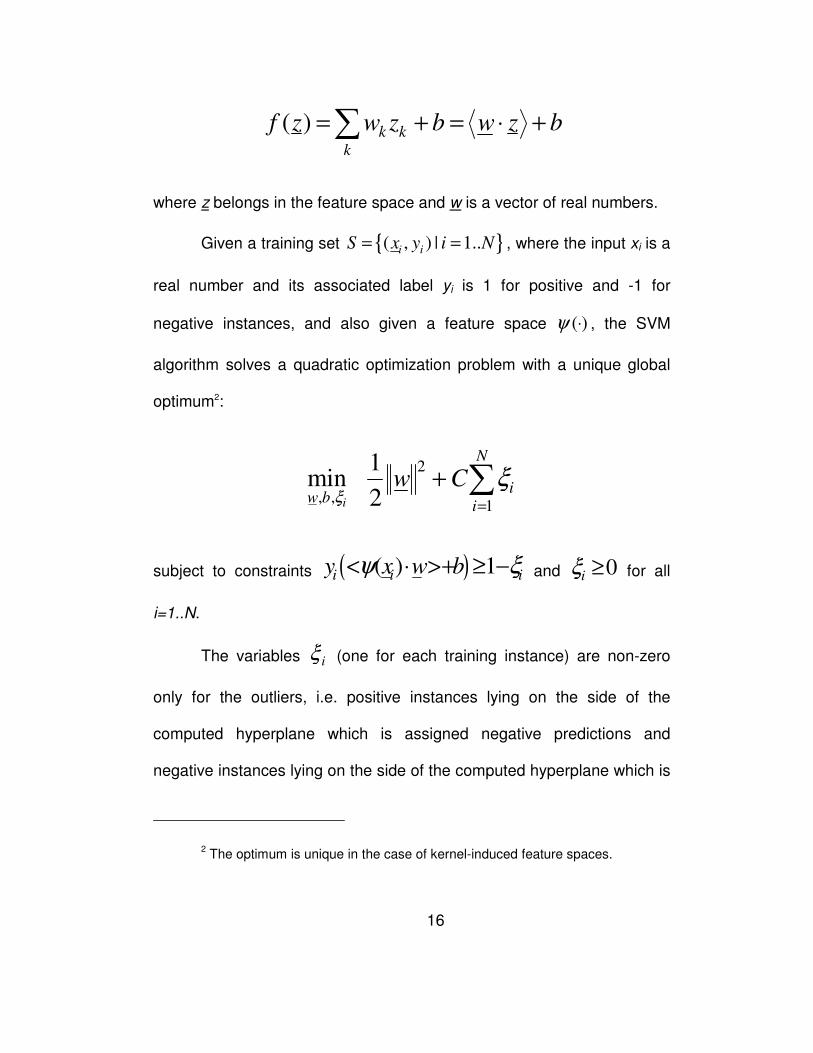
16
( ) k k
k
f z w z b w z b= + = ⋅ +∑
where z belongs in the feature space and w is a vector of real numbers.
Given a training set { }( , ) | 1..i iS x y i N= = , where the input xi is a
real number and its associated label yi is 1 for positive and -1 for
negative instances, and also given a feature space )(⋅ψ , the SVM
algorithm solves a quadratic optimization problem with a unique global
optimum2:
2
, ,1
1min
2i
N
iw b
i
w Cξ
ξ=
+ ∑
subject to constraints ( )( ) 1i i iy x w bψ ξ< ⋅ >+ ≥ − and 0≥iξ for all
i=1..N.
The variables iξ (one for each training instance) are non-zero
only for the outliers, i.e. positive instances lying on the side of the
computed hyperplane which is assigned negative predictions and
negative instances lying on the side of the computed hyperplane which is
2 The optimum is unique in the case of kernel-induced feature spaces.

17
assigned positive predictions. The parameter C establishes a tradeoff
between the total effect of outliers and the maximum achievable margin.
In order to see that there is actually such a tradeoff, observe that the
margin can be arbitrarily increased by simply allowing room for an
increasing number of outliers.
The optimization problem is solved by a transformation to its
corresponding dual form and the solution is given in terms of the
Lagrangian multipliers iα of the dual problem:
1
( ) ( ) ( )N
i i i
i
f x y x x bα ψ ψ=
= < ⋅ > +∑
It is worth noting that iα is non-zero only for support vectors and
therefore only those instances contribute to the sum. Also, in practice,
the dot product of the instance with each training example
( ) ( )ix xψ ψ< ⋅ > can be efficiently computed using special similarity
functions called kernels, where the computation takes place in the input
space and therefore mapping the instances to the feature space (whose
dimensionality is much higher, sometimes infinite) is not necessary.
Thus, if ( , )K ⋅ ⋅ is a kernel function inducing the feature space )(⋅ψ , and
18
SV S⊆ is the set of support vectors, the previous equation can be
rewritten as:
( ) ( , )
i
i i i
x SV
f x y K x x bα∈
= +∑
The final hypothesis h for binary classification is obtained by
taking the sign of f:
( ) sgn ( )h x f x=
As with the boosting algorithm, several SVM extensions, including
the introduction of new notions of margin and variations of the original
quadratic optimization problem, have been proposed for solving a variety
of learning problems, such as hierarchical classification [33], clustering
[34], one-class SVM [35], and structured classification [36, 37]. In this
thesis, one-class SVM is used for horizontal gene transfer detection
(chapter 3) and multi-class SVM (based on all-against-all binary SVM
classifiers) for protein sub-cellular localization prediction (chapter 4).
19
3 Horizontal Gene Transfer
In recent years, the increase in the amounts of available genomic
data has made it easier to appreciate the extent by which organisms
increase their genetic diversity through horizontally transferred genetic
material. Such transfers have the potential to give rise to extremely
dynamic genomes where a significant proportion of their coding DNA has
been contributed by external sources. Because of the impact of these
horizontal transfers on the ecological and pathogenic character of the
recipient organisms, methods are continuously sought that are able to
computationally determine which of the genes of a given genome are
products of transfer events. In this thesis, we introduce and discuss a
novel computational method for identifying horizontal transfers that relies
on a gene’s nucleotide composition and obviates the need for knowledge
of codon boundaries. In addition to being applicable to individual genes,
the method can be easily extended to the case of clusters of horizontally
transferred genes. With the help of an extensive and carefully designed
set of experiments on 123 archaeal and bacterial genomes, we
20
demonstrate that the new method exhibits significant improvement in
sensitivity when compared to previously published approaches. In fact, it
achieves an average relative improvement across genomes of between
11% and 41% compared to the Codon Adaptation Index method in
distinguishing native from foreign genes. Our method’s horizontal gene
transfer predictions for 123 microbial genomes are available online at
http://cbcsrv.watson.ibm.com/HGT/.
3.1 Related work
As early as 1944, scientists began accumulating experimental
evidence on the ability of microbes to uptake “naked” DNA from their
environment and incorporate it into their genome [38]. Several years
later, in 1959, plasmids carrying antibiotic resistance genes were shown
to spread among various bacterial species. And as the 20th century
came to a close, there was increased appreciation of the fact that genes
found in mitochondria and chloroplasts are often incorporated in the
nuclear genome of their host organism [39-41]. Nonetheless, there have
been intense debates through the years on the possibility that the
transfer of genetic material among different species may play a
21
significant role in evolution. This process is known as horizontal gene
transfer (HGT), or, equivalently, lateral gene transfer (LGT).
Before the advent of the genomics era, only a handful of
horizontal gene transfer events were documented in the literature [42].
And even though it had been argued that gene acquisition from foreign
species could potentially have a great impact on evolution [43], it was not
until after the genomic sequences of numerous prokaryotic and
eukaryotic organisms became publicly available that the traditional tree-
based evolutionary model was seriously challenged, considering even
the possibility of substantial gene exchange [44, 45]. In particular, it was
first observed that some Escherichia coli genes exhibit codon
frequencies that deviate significantly from those of the majority of its
genes [46]. Also, the genomes of A. aeolicus and T. maritima, two
hyperthermophilic bacteria, supported the hypothesis of a massive gene
transfer from archaeal organisms with which they shared the same
lifestyle [47, 48].
Subsequent phylogenetic studies at a genomic scale have
demonstrated that the archaeal proteins can be categorized into two
distinct groups with bacterial and eukaryotic homologues [49-51].
Incidentally, and in full agreement with the model of early evolution
22
whereby eukaryotes and archaea descended from a common ancestor,
the so-called informational genes (involved in translation, transcription
and replication) exhibit eukaryotic affinity, whereas metabolic enzymes,
structural components and uncharacterized proteins seem to be
homologous to bacterial genes.
The significance of horizontal gene transfer goes beyond helping
interpret phylogenetic incongruencies in the evolutionary history of
genes. In fact, there is strong evidence that pathogenic bacteria can
develop multi-drug resistance simply by acquiring antibiotic resistance
genes from other bacteria [52, 53]. More evidence of gene transfer as
well as a detailed description of the underlying biological mechanisms
can be found in [54, 55]. And in [56], the authors present a quantitative
estimate of this phenomenon in prokaryotes and propose a classification
comprising two distinct types of horizontal gene transfer.
Several methods have been devised for the identification of
horizontally acquired genes. Traditionally, phylogenetic methods have
been used to prove that a gene has been horizontally transferred [55].
These methods work well when sufficient amounts of data are available
for building trees with good support; but very frequently this is not the
case and other approaches need to be exploited in order to identify
horizontally-transferred genes in the genome under consideration.
23
Examples of such approaches include the unexpected ranking of
sequence similarity among homologs where genes from a particular
organism show the strongest similarity to a homolog from a distant taxon
[56], gene order conservation in operons from distant taxa [57, 58], and
atypical nucleotide composition [59].
Previously published methods for horizontal gene transfer
detection were based on gene content and operated under the
assumption that in a given organism there exist compositional features
that remain relatively constant across its genomic sequence. Genes that
display atypical nucleotide composition compared to the prevalent
compositional features of their containing genome are likely to have been
acquired through a horizontal process. Consequently, over the years, a
number of features have been proposed for defining ‘signatures’ that
would be characteristic for a genome: any gene deviating from the
signature can be marked as a horizontal transfer candidate. We
continue with a brief summary of the various signatures that have been
discussed in the literature.
The simplest and historically earliest type of proposed genomic
signature is a genome’s composition in terms of the bases G and C,
known as the genome’s G+C content [59]. It is important to note that
due to the periodicity of the DNA code, as this periodicity is implied by
24
the organization of the coding regions into codons, the G+C content
varies significantly as a function of the position within the codon. As a
result, four discrete G+C content signatures can be identified. The first
corresponds to the overall G+C content and is computed by considering
all of the nucleotides in a genome. Each of the remaining three
signatures, denoted by G+C(k), with k=1,2,3, corresponds to the value of
the G+C content as the latter is determined by considering only those
nucleotides occupying the k-th position within each codon; unlike the
G+C signature which is computed across all genomic positions, only
coding regions are used in the computation of G+C(k).
A related variation of the G+C(k) content idea is the so-called
Codon Adaptation Index (CAI) which was introduced in [60]. CAI
measures the degree of correlation between a given gene’s codon usage
and the codon usage that is deduced by considering only highly
expressed genes from the organism under consideration.
In yet another variation introduced in the context of a study of the
Escherichia coli genome, Lawrence and Ochman [61] identified atypical
protein coding regions by simultaneously combining G+C(1) and G+C(3).
Moreover, and for each gene in turn, they computed a ‘codon usage’ that
assessed the degree of bias in the use of synonymous codons compared
to what was expected from each of the three G+C(k) values. A gene
25
was rendered atypical when its relative ‘codon usage’ - as defined above
- differed significantly from its CAI value.
The codon usage patterns in Escherichia coli were also
investigated by Karlin et al in [62] who found that the codon biases
observed in ribosomal proteins deviate the most from the biases of the
average Escherichia coli gene. Using this observation, they defined
‘alien’ genes as those genes whose codon bias was high relative to the
one observed in ribosomal proteins and also exceeded a threshold when
compared to that of the average gene.
Another popular genomic signature is the relative abundance of
dinucleotides compared to single nucleotide composition. Despite the
fact that genomic sequences display various kinds of internal
heterogeneity including G+C content variation, coding versus non-
coding, mobile insertion sequences, etc., they nonetheless preserve an
approximately constant distribution of dinucleotide relative-abundance
values, when calculated over non-overlapping 50-kb-wide windows
covering the genome; this observation was demonstrated by Karlin et al
in [63, 64]. But more importantly, the dinucleotide relative-abundance
values of different sequence samples of DNA from the same or from
closely related organisms are generally much more similar to each other
than they are to sequence samples from other organisms. In related
26
work, Karlin and co-workers introduced the ‘codon signature,’ which was
defined as the dinucleotide relative abundances at the distinct codon
positions 1-2, 2-3 and 3-4 (4 = 1 of the next codon) [65]: for large
collections of genes (50 or more), they showed that this codon signature
is essentially invariant, in a manner analogous to the genome signature.
A genomic signature comprising higher-order nucleotides was
proposed by Pride and Blaser in [66], where the observed frequencies of
all n-sized oligonucleotides in a gene are contrasted against their
expected frequencies estimated by the observed frequencies of (n-1)-
sized oligonucleotides in the host genome. In the accompanying
analysis, the authors focused on identifying horizontally transferred
genes in Helicobacter pylori, and for that genome they showed that
signatures based on tetranucleotides exhibit the best performance,
whereas higher-order oligonucleotides did not result in any improvement.
However, since their analysis was based on a single genome, it is not
possible to deduce any generally applicable guidelines.
In [67], Hooper and Berg propose as a genomic signature the
dinucleotide composed of the nucleotide in the third codon position and
the first position nucleotide of the following codon. Using the 16 possible
dinucleotide combinations, they calculate how well individual genes
conform to the computed mean dinucleotide frequencies of the genome
27
to which they belong. Mahalanobis distance, instead of Euclidean, is
used to generate a distance measure on the dinucleotide distribution. It
was also found that genes from different genomes could be separated
with a high degree of accuracy using the same distance.
Sandberg et al. investigated the possibility of predicting the
genome of origin for a specific genomic sequence based on the
differences in oligonucleotide frequency between bacterial genomes [68].
To this end, they developed a naïve Bayesian classifier and
systematically analyzed 28 eubacterial and archaeal genomes, and
concluded that sequences as short as 400 bases could be correctly
classified with an accuracy of 85%. Using this classifier they
demonstrated that they could identify horizontal transfers from
H influenzae to N. meningitis.
Hayes and Borodovsky demonstrated the connection between
gene prediction and atypical gene detection in [69]. Working with
bacterial species, they addressed the problem of accurate statistical
modeling of DNA sequences and observed that more than one statistical
model were needed to describe the protein-coding regions. This was the
result of diverse oligo-nucleotide compositions among the protein-coding
genes and in particular of the variety of their codon usage strategies. In
the simplest case, two models sufficed, one capturing typical and the
28
other atypical genes. Clearly, the latter model also allowed the
identification of good horizontal transfer candidates. Along similar lines,
Nakamura et al. [70] recently conducted a study of biological functions of
horizontally transferred genes in prokaryotic genomes. Their work did not
introduce a new computational method but rather applied anew the
method originally introduced by Borodovksi et. al. [71] in the context of
gene finding. In a manner analogous to deciding whether a given ORF
corresponds to a gene, Nakamura et al. determined whether a given
gene was horizontally transferred and compiled and reported results for
a total of 116 complete genomes.
In [72], the authors identified horizontal gene transfer candidates
by combining multiple identification methods. Their analysis is based on
a hybrid signature that includes G+C and G+C(k) content, codon usage,
amino-acid usage and gene position. Genes whose G+C content
significantly deviates from the mean G+C content of the organism are
candidate gene transfers provided they also satisfy the following
constraints: a) they have an unusual codon usage (computed in a similar
way); b) their length exceeds 300bp; and c) their amino-acid composition
deviates from the average amino-acid composition of the genome.
However, the authors stressed the need to exclude highly expressed
genes from the set of candidate transfers: such genes may deviate from
29
the mean values of codon usage simply because of a need to adapt so
as to reflect changes in tRNA abundance. As an example, ribosomal
proteins are filtered out and are not included in the list of predictions.
Similar in flavor, the method described in [73] applies several
approaches simultaneously, for example, G+C content, codon and
amino-acid usage, and generates results for 88 complete bacterial and
archaeal genomes. The putative horizontally transferred genes are
collected and presented in the HGT-DB database that is accessible on-
line.
The methods in [72, 73] do not introduce a new genomic
representation scheme but rather combine several distinct modalities into
one feature vector. As is always the case with feature vectors
comprising distinct and non-uniform features, it is difficult to derive a
distance function that properly takes into account the different units, the
different ranges of values, etc. Notably, and in direct contrast to this
approach, our proposed method which is outlined below uses a single
feature in order to determine whether a gene is indigenous to a genome
or not.
In [74], surrogate methods for detecting lateral gene transfer are
defined as those that do not require inference of phylogenetic trees.
Four such methods were used to process the genome of Escherichia coli
30
K12. Only two of these methods detect the same ORFs more frequently
than expected by chance, whereas several intersections contain many
fewer ORFs than expected.
Finally, we should mention an approach that is radically distinct
from the ones described above. In [75], Ragan and Charlebois organize
ORFs from different genomes in groups of high sequence similarity
(using gapped BLAST) and look at the distributional profile of each group
across the genomes. Those ORFs whose distribution profile cannot be
reconciled parsimoniously with a tree-like descent and loss are likely
instances of horizontal gene transfer. In other words, instead of deciding
whether a gene is typical or atypical by comparing its composition to that
of the containing genome, they perform a statistical comparison of similar
genes across genomes.
In what follows, we present a novel methodology that exploits
genomic composition to discover putative horizontal transfers. Notably,
our method does not require knowledge of codon boundaries. By
carrying out a very extensive set of experiments with 123 archaeal and
bacterial genomes, we demonstrate that our method significantly
outperforms previously published approaches including the Codon
Adaptation Index (CAI), C+G and all its variants as well as methods
based on dinucleotide frequencies.
31
3.2 Generalized compositional features
Our proposed approach extends and generalizes composition-
based methods in three distinct ways:
• first, we advocate the use of higher order nucleotide sequences
(templates) so as to overcome the diminished discrimination
power exhibited by the previously proposed di- and tri-nucleotide
models. Our use of richer compositional features is expected to
lead to an increased ability in identifying genes with atypical
compositions and thus an improved ability to classify;
• that include ‘wildcards’ and thus do not comprise consecutive
nucleotides. Wildcards are indicated with the help of a “dot” or
“don’t care” character: any nucleotide that occupies the “don’t
care” position will be ignored during the computation of the
signature. As an example, the template A.G will match any of
AAG, ACG, AGG, or ATG, while ignoring the identity of the
nucleotide occupying the middle position; and,
• third, we optionally take into account the periodicity of the DNA
code; in particular, when collecting the instances of a template, we
can impose the constraint that a template be position-specific.
32
For example, when calculating the codon frequencies, the tri-
nucleotide templates to be considered are only the ones that start
at positions 3k+1, where k is a non-negative integer.
In our augmented model, let us denote the compositional feature
vector for any given DNA sequence s over a set of templates π = { π1,
π2, ..., πq } as ( )q21 ..., , ,)( αααφ =s ; here αi is the frequency of
template πi in sequence s.
Instead of using the absolute template frequencies, we also
considered normalizing these frequencies over the expected template
frequencies: the latter can be derived from the single nucleotide
composition with respect to some background reference sequence under
the assumption of an i.i.d. model. Typically, if the sequence of interest is
a gene g, or a DNA fragment belonging to a genome G, the single
nucleotide frequencies of genome G ought to also reflect the expected
single nucleotide frequencies of an endogenous gene g. The relative
(normalized) frequencies are thus given by the following equation:
∏ =
=i
j ijG
ig
i
P
P
ππ
πα
1)(
)(
33
where πij is the j-th nucleotide of template πi, Pg(i) is the observed
frequency of template πi in gene Gg ∈ , whereas the single nucleotide
probabilities PG(ij) in the denominator are computed from the entire
genome G, and we can choose to make them position-specific or not.
The probability of the ‘dot’ character is one.
3.2.1 From compositional features to gene typicality scores
Given a genome sequence, our ultimate objective is to
characterize the genes in the genome in terms of how “atypical” they are.
Under the assumption that any given genome exhibits a relatively
constant composition over intervals that may not be contiguous, genes
whose template composition differs substantially from the typical
composition of their host genome are likely to have been acquired
through a horizontal transfer event. In our work, we assign a typicality
score SG(g) to each gene g of genome G: the higher the score the more
typical the gene is for the genome. Consequently, genes with low scores
will correspond to gene transfer candidates.
A straightforward approach towards the computation of a gene’s
typicality score given its feature vector φ(g) is to compare it to the feature
vector φ(G) for the whole genome. The comparison can be performed in
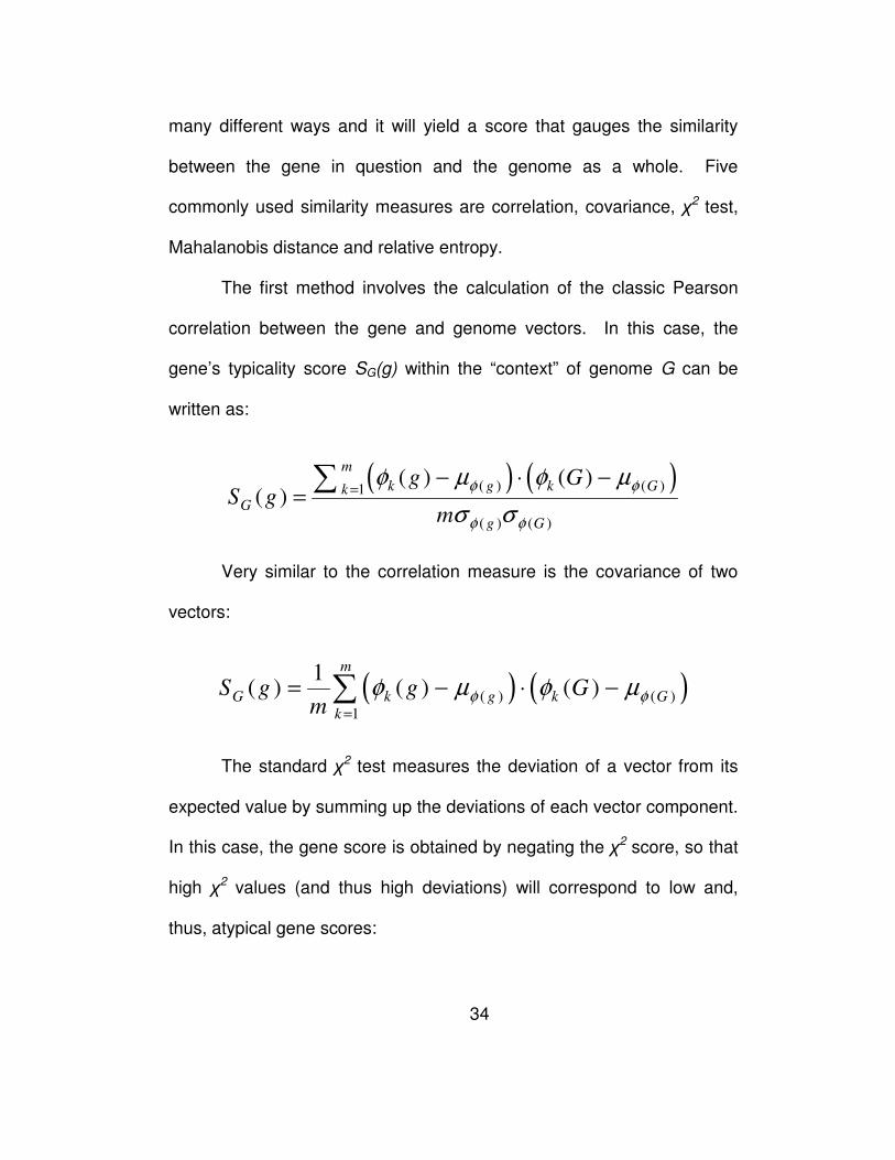
34
many different ways and it will yield a score that gauges the similarity
between the gene in question and the genome as a whole. Five
commonly used similarity measures are correlation, covariance, χ2 test,
Mahalanobis distance and relative entropy.
The first method involves the calculation of the classic Pearson
correlation between the gene and genome vectors. In this case, the
gene’s typicality score SG(g) within the “context” of genome G can be
written as:
( ) ( )( ) ( )1
( ) ( )
( ) ( )( )
m
k g k GkG
g G
g GS g
m
φ φ
φ φ
φ µ φ µ
σ σ=
− ⋅ −=∑
Very similar to the correlation measure is the covariance of two
vectors:
( ) ( )( ) ( )
1
1( ) ( ) ( )
m
G k g k G
k
S g g Gm
φ φφ µ φ µ=
= − ⋅ −∑
The standard χ2 test measures the deviation of a vector from its
expected value by summing up the deviations of each vector component.
In this case, the gene score is obtained by negating the χ2 score, so that
high χ2 values (and thus high deviations) will correspond to low and,
thus, atypical gene scores:
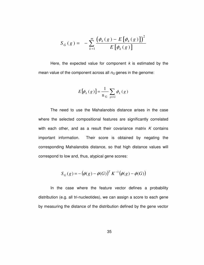
35
[ ]( )[ ]
2
1
( ) ( )( )
( )
mk k
G
k k
g E gS g
E g
φ φ
φ=
−= − ∑
Here, the expected value for component k is estimated by the
mean value of the component across all nG genes in the genome:
[ ] ∑∈
=Gg
kk ggE )(n
1 )(
G
φφ
The need to use the Mahalanobis distance arises in the case
where the selected compositional features are significantly correlated
with each other, and as a result their covariance matrix K contains
important information. Their score is obtained by negating the
corresponding Mahalanobis distance, so that high distance values will
correspond to low and, thus, atypical gene scores:
( ) ( ))()()()( )(1
GgKGggST
G φφφφ −−−= −
In the case where the feature vector defines a probability
distribution (e.g. all tri-nucleotides), we can assign a score to each gene
by measuring the distance of the distribution defined by the gene vector
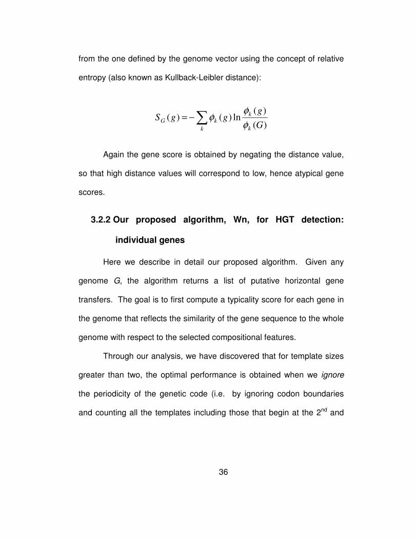
36
from the one defined by the genome vector using the concept of relative
entropy (also known as Kullback-Leibler distance):
)(
)(ln)( )(
G
gggS
k
k
k
kGφ
φφ∑−=
Again the gene score is obtained by negating the distance value,
so that high distance values will correspond to low, hence atypical gene
scores.
3.2.2 Our proposed algorithm, Wn, for HGT detection:
individual genes
Here we describe in detail our proposed algorithm. Given any
genome G, the algorithm returns a list of putative horizontal gene
transfers. The goal is to first compute a typicality score for each gene in
the genome that reflects the similarity of the gene sequence to the whole
genome with respect to the selected compositional features.
Through our analysis, we have discovered that for template sizes
greater than two, the optimal performance is obtained when we ignore
the periodicity of the genetic code (i.e. by ignoring codon boundaries
and counting all the templates including those that begin at the 2nd and

37
3rd codon positions), use no wildcards in the templates, and by choosing
covariance as the similarity measure for computing the final scores. We
use Wn to denote our method, where n is greater that two and is equal to
the size of the template. An example of a template is shown in Figure 1.
It should be stressed here that, allowing representations based on
generalized templates comprising both gap and non-gap characters
seems to yield no further improvement for the particular set of genomes
we experimented with. Nonetheless we can expect that, as the
sequences of more complete genomes become available, the additional
flexibility provided by the gapped templates that we introduced in this
work has the potential of further improving performance.
We observed that the performance of our method increased with
the size of the template, reaching a maximum at size 8; increasing the
size of the template further resulted in a sharp drop of performance.
With respect to the choice of template size one needs to keep in mind
that higher template sizes will result in greater specificity provided of
course that the regions of DNA being processed can yield a sufficient
percentage of non-zero counts. As a rule of thumb, smaller size
templates should be used when individual gene transfers are sought,
whereas larger size templates can be chosen when attempting to identify
38
clusters of horizontally transferred genes, which in turn can be done by
using the sliding window method described below.
3.2.3 Our proposed algorithm, Wn, for HGT detection:
clusters of transferred genes
For completeness, we now describe a modification of the
proposed Wn algorithm that can be applied to the problem of detecting
clusters of putative gene transfers: instead of computing the feature
vectors over individual genes, the computation is now applied on sliding
windows that span multiple, neighboring genes. The size of the window
is given in terms of the number of genes that it spans and not in terms of
a nucleic acid span: the number of genes to be included in the
computation is a parameter in this modified version of our algorithm,
while n of course still denotes the template size. For each such window,
we obtain a score: the score of a given gene within the window is
computed as the average of the scores of all of the windows that include
the gene in question. In the next section, we discuss the application of
our algorithm on the genome of Enterococcus faecalis which contains a
known cluster of horizontally transferred genes conferring vancomycin-
resistance.
39
3.2.4 Our proposed algorithm, Wn, for HGT detection:
automated threshold selection
Given the typicality scores that Wn computes for each gene of a
genome, we need to be able to automatically determine a threshold
value: all genes with scores below it are considered to be horizontal
transfers. We illustrate our automated threshold selection methodology
with the help of the genome of A pernix. The distribution of the obtained
scores f, sorted in order of increasing values, is shown in Figure 2. In
the same figure, we also show the derivative f’ of the distribution,
properly smoothed by taking the average over sliding windows and
normalized so that its values range from zero to one.
It can be seen that the scores increase very fast for the first few
genes, but once we make the transition from atypical genes to genes of
higher typicality the derivative remains approximately constant. It is
precisely at this point that we set the threshold value T on the derivative
f’. With the score threshold having been decided automatically, we
define the number NHGT of predicted horizontal gene transfers to be the
smallest value i for which the derivative of the ranked scores becomes
equal to the threshold T: clearly these NHGT lowest scoring genes
comprise our list of putative gene transfers.
40
3.2.5 Results
In order to assess the potential of using compositional features in
the detection of horizontal gene transfers in a host genome, we designed
and carried out a very large number of experiments that simulated gene
transfer. The experimental procedure has as follows: we created a pool
of donor genes, and randomly subselected an appropriate fraction of
these genes that were then incorporated into the bacterial or archaeal
host genome under consideration. The task at hand is that of recovering
as many as possible of the inserted donor genes.
It is important to note that, unlike previously proposed random
experiments where artificial genes were produced as random sequences
which obeyed some very general statistics (e.g. a given observed
mononucleotide frequency distribution), our simulations are carried out
using real genes and thus are realistic simulations of what happens in
nature (as we currently understand it). Constructing and using random
sequences to simulate gene transfers is simply not a valid approach.
We have carried out experiments with two distinct pools of donor
genes. The first pool was built from the gene complement of the 27
phages that are shown in Table 1 and comprised 1,485 genes. The
41
second pool comprised more than 350,000 archaeal and bacterial genes
and is discussed later in this section. In both sets of experiments, we
used as “host” genomes a collection of 123 fully sequenced prokaryotic
genomes (archaea and bacteria), which we downloaded from the
NCBI/NIH ftp server.
3.2.5.1 Case 1: donor pool comprising phage genes
For each of the 123 host organisms in turn, we conducted k=100
experiments of simulated transfers from the pool of phage genes into the
genome of the host organism. In each case, the number of added genes
was chosen to be a fixed percentage of the number of genes in the host
genome. The “transferred” genes were selected from the donor pool at
random and with replacement. So as to be more realistic, we carried out
the simulated-transfer-experiment for transfer percentages that ranged
between 1% and 8% of the genes in the host genome at hand. For each
genome and transfer percentage combination, the task was that of
recovering as many of the artificially transferred genes as possible,
without using any a priori knowledge about the host genome or the donor
genes. For the genome and percentage combination being considered,
we accumulated results from over 100 repetitions of the transfer-and-
recover experiment and reported the arithmetic average.
42
In the ideal case, a method ought to be able to recover every
single one of the added genes. But the reader should keep in mind that
our artificially transferred genes compete with all of the bona fide
horizontal transfers, already-present in the genome under consideration,
for the same top putative-transfer positions. Nonetheless, this situation
poses no problem for the purposes of simulation as it holds true for all of
the tested methods, and thus no method is favored at the expense of
another.
Each tested method computes a “typicality” score for each gene
based on different gene features each time. Let ρ be the number of
genes that we artificially added to the genome being studied: the various
methods are evaluated according to their “hit ratio,” which is defined as
the percentage of artificially-added genes occupying the ρ-lowest
typicality score values. In other words, we measure how many of the
artificial transfers end up occupying the ρ-lowest positions. Clearly, the
more successful a method is in discovering gene transfers, the closer the
computed hit ratio will be to 100%. If m denotes a gene-scoring method,
G the genome under consideration, and )(Grm
i the hit ratio obtained
by the method m at the i-th iteration of the experiment (with ki ≤≤1 ),
then we can define the performance m
GPerf of method m on genome G
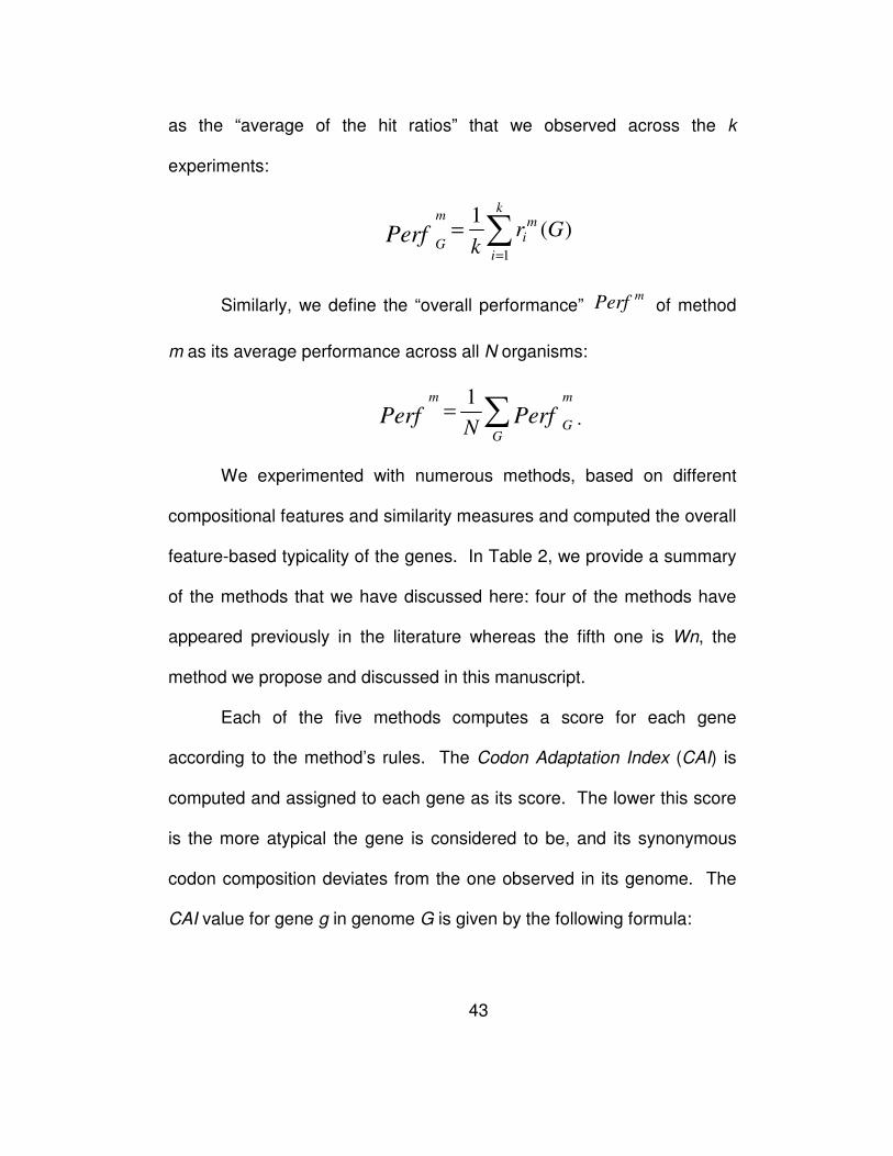
43
as the “average of the hit ratios” that we observed across the k
experiments:
∑=
=k
i
mi
m
GGr
kPerf
1
)(1
Similarly, we define the “overall performance” m
Perf of method
m as its average performance across all N organisms:
∑=G
m
G
m
PerfPerfN
1.
We experimented with numerous methods, based on different
compositional features and similarity measures and computed the overall
feature-based typicality of the genes. In Table 2, we provide a summary
of the methods that we have discussed here: four of the methods have
appeared previously in the literature whereas the fifth one is Wn, the
method we propose and discussed in this manuscript.
Each of the five methods computes a score for each gene
according to the method’s rules. The Codon Adaptation Index (CAI) is
computed and assigned to each gene as its score. The lower this score
is the more atypical the gene is considered to be, and its synonymous
codon composition deviates from the one observed in its genome. The
CAI value for gene g in genome G is given by the following formula:
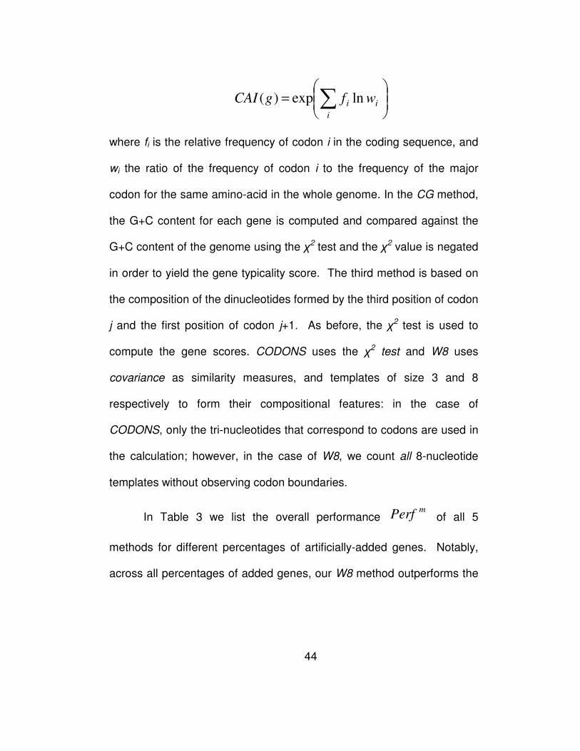
44
= ∑
i
ii wfgCAI lnexp )(
where fi is the relative frequency of codon i in the coding sequence, and
wi the ratio of the frequency of codon i to the frequency of the major
codon for the same amino-acid in the whole genome. In the CG method,
the G+C content for each gene is computed and compared against the
G+C content of the genome using the χ2 test and the χ2 value is negated
in order to yield the gene typicality score. The third method is based on
the composition of the dinucleotides formed by the third position of codon
j and the first position of codon j+1. As before, the χ2 test is used to
compute the gene scores. CODONS uses the χ2 test and W8 uses
covariance as similarity measures, and templates of size 3 and 8
respectively to form their compositional features: in the case of
CODONS, only the tri-nucleotides that correspond to codons are used in
the calculation; however, in the case of W8, we count all 8-nucleotide
templates without observing codon boundaries.
In Table 3 we list the overall performance mPerf of all 5
methods for different percentages of artificially-added genes. Notably,
across all percentages of added genes, our W8 method outperforms the
45
rest. The entries of Table 3 are also shown in Figure 3a in the form of a
plot.
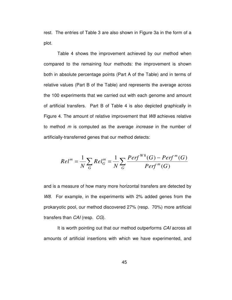
Table 4 shows the improvement achieved by our method when
compared to the remaining four methods: the improvement is shown
both in absolute percentage points (Part A of the Table) and in terms of
relative values (Part B of the Table) and represents the average across
the 100 experiments that we carried out with each genome and amount
of artificial transfers. Part B of Table 4 is also depicted graphically in
Figure 4. The amount of relative improvement that W8 achieves relative
to method m is computed as the average increase in the number of
artificially-transferred genes that our method detects:
81 1 ( ) ( )
( )
W mm m
G mG G
Perf G Perf GRel Rel
N N Perf G
−= =∑ ∑
and is a measure of how many more horizontal transfers are detected by
W8. For example, in the experiments with 2% added genes from the
prokaryotic pool, our method discovered 27% (resp. 70%) more artificial
transfers than CAI (resp. CG).
It is worth pointing out that our method outperforms CAI across all
amounts of artificial insertions with which we have experimented, and
46
exhibits significant relative improvements that range between 11% and
41%. Equally important is the fact that our method exhibits much greater
sensitivity and shows a very significant advantage over all of the earlier
methods when the number of horizontally transferred genes is small
compared to the number of genes in the host genome.
Figure 5 shows a detailed analysis of the performance of W8
compared to the CAI method for each of the 123 genomes and for those
experiments where we added 2% donor genes. In this Figure use green
colored bars for those genomes in which W8 outperforms CAI, and a
red-colored bar if the opposite holds true. The height of each bar shows
the magnitude of the relative improvement mGRel achieved by our
method over CAI as an average over the 100 experiments and can be
either positive (green bars) or negative (red bars). As can be seen here,
for the majority of the organisms (91 vs. 32) the W8 method recovers
more of the artificially inserted genes than CAI does. But more
importantly, W8 does so while achieving a significantly higher relative
improvement margins than CAI.
Next, we exhaustively studied the impact that the size of the
template has on the overall performance. Using the same experimental
protocol as above and carrying out 100 experiments per organism, we
47
observed that for template sizes greater than 2, the optimal performance
is achieved when we ignore codon boundaries and use covariance to
compute the similarity scores. Figure 7a shows atypical gene detection
performance as a function of the employed template size. It is evident
from this figure that an increase in template size leads to continuous
increase in performance reaching a maximum for template sizes
between 6 and 8 inclusive. In fact, the performance is nearly identical for
these three template sizes. Any further increase in the template size
leads to a quick drop in performance.
3.2.5.2 Case 2: donor pool comprising genes from
archaeal and bacterial genomes.
We also repeated the above experiments but this time the pool
from which the donor genes were selected comprised the approximately
350,000 genes from the 123 genomes that we used as hosts. In other
words, we effectively simulated the case where our host genomes could
exchange genes with one another in any conceivable combination. To
the best of our knowledge, this kind of simulation has not been
previously used in the context of evaluating a horizontal gene transfer
method. Naturally, we added a bookkeeping stage in this simulation that
48
ensured that all the genes that were artificially inserted in genome G
originated in genomes other than G.
In order to account for the bigger size of the donor pool, we
conducted k=1000 repetitions for each artificial transfer experiment. In
Figure 3b, we show the overall performance of the five evaluated
methods as a function of the percentage of added genes, and in Figure 6
we plot the relative improvement achieved in each genome by our
method compared to CAI. Finally, the effect that changing the template
size has on performance is shown in Figure 7b. Not surprisingly, the
results obtained during the simulation with the prokaryotic donor pool are
in agreement with those obtained from the simulation with the phage
donor gene pool.
There still remains the issue of which of the three best-performing
template sizes to use. This depends on the expected size of the DNA
fragment that will be processed. Given that the sensitivity achieved by
template sizes 6 through 8 is virtually the same, use of the largest
possible template size will allow us to achieve greater specificity,
provided of course that the regions of DNA under consideration can
generate a substantial number of non-zero counts. As a rule of thumb,
we propose that smaller template sizes be used when isolated gene
49
transfers are sought. Larger size templates will be more appropriate
when attempting to identify clusters of horizontally transferred genes.
We conclude by applying the sliding-window version of our
algorithm to the genome of Enterococcus faecalis, where a cluster of
vancomycin resistance related genes is known to have been horizontally
transferred. As a matter of fact, in Enterococcus faecalis V583 there is a
cluster of seven genes, EF2293-EF2299, that confers vancomycin
resistance to Enterococcus faecalis. Using the sliding window version of
our method over windows of 5 consecutive genes, and template sizes
that ranged from 6 through 11 inclusive, we computed scores for each of
of Enterococcus faecalis’ genes. CAI values were also generated for the
same gene collection. Our goal was to compare the atypicality ranks of
the genes that are known to be horizontal transfers as these ranks would
be deduced by each of five scoring methods. As stated above, the lower
the score of a gene (equivalently: the lower the gene’s rank), the more
atypical it is considered to be. Given the cluster’s common origin, the
ideal method should be able to report this collection as a group with no
other genes achieving atypicality scores within the range of values
spanned by the cluster’s genes. Moreover, the ideal method should be
able to assign as low scores as possible to this collection emphasizing its
horizontally transferred nature. In Figure 8, we show the results of the
50
gene ranks produced by some of the methods. As can be seen here,
W6 through W8 perform equally well. The span of gene ranks for the
cluster’s members is low for template sizes 6 through 8 and equal to the
span obtained by the CAI method. As anticipated, W8 outperforms CAI
by reporting the genes of this cluster earlier in the list of putative
horizontal transfers – this is indicated by the overall lower rank values
which are assigned to the cluster as a whole. Further increasing the
specificity of the employed templates by increasing their size results in
earlier reporting of the vancomycin cluster in the list of candidate
transfers. But this is achieved at the expense of increasingly losing the
score coherence which is expected given that the genes under
consideration are part of the same logical unit. This last experiment
further corroborates the conclusion reached during our artificial-insertion
experiments that a template size of 8 nucleotides (i.e. W8 method)
represents an optimal choice for Wn.
3.2.6 Discussion
In this chapter we introduced and discussed a new, composition-
based framework for the detection of horizontal gene transfers. Our
proposed method, Wn, is based on compositional features but extends
51
and generalizes all previously proposed schemes. Wn works by
assigning a typicality score to each gene that reflects the gene’s
similarity with the containing genome as this is gauged by the features in
use. We have also described a way to automatically determine a
typicality score threshold was also described. Finally, an extension of
Wn for the case where the sought transfers are likely to appear in
clusters (as opposed to isolated genes) was also described and
discussed. We have created a web-site comprising the predictions of the
horizontal gene transfers for all 123 archaeal and bacterial genomes
based on our method at http://cbcsrv.watson.ibm.com/HGT/.
We carried out a comparative evaluation of Wn and previously-
reported computational methods for the discovery of horizontal gene
transfers. In particular, we evaluated five representative methods by
inserting random, varying-size collections of phage and prokaryotic
genes in each of 123 host genomes (archaea and bacteria) and
processing those artificially-created genomes with each method. Our
objective was to recover in the lowest-scoring positions (highly atypical
genes) as many of the added phage genes as possible without making
use of any a priori knowledge about either the host organism or the
inserted genes. These experiments as well as the study of a specific,
documented case from Enterococcus faecalis strongly demonstrated that
52
templates with sizes ranging from 6 to 8 nucleotides yield optimal
performance.
We also reported on pairwise comparisons of Wn with the CAI
and G+C methods and for each of 123 genomes in turn. Combining the
results across all 123 genomes, W8 clearly outperformed both CAI and
G+C. W8 achieved very significant relative improvements over CAI that
averaged 25%. The relative improvements over G+C were even more
pronounced.
Arguably, for many years, the essence of computational methods
that relied on genomic DNA alone to draw conclusions on horizontal
gene transfers had remained largely unchanged. In this light, our
proposed method is of particular relevance: it is very fast, it need only
access the genomic DNA in question (i.e. partial or whole sequence of
host genome and partial or whole sequence of candidate stretch of
DNA), it obviates the need for access to databases of genomic
sequences, it obviates the need for comparative analyses with other
genomes, and finally, it does not make use of any codon boundary
knowledge. Despite the minimal amounts of information that our method
uses, a very extensive series of computational experiments on one
hundred and twenty-three (123) genomes amply demonstrated the
53
superiority of our method which achieved a relative improvement of
between 11% and 41% over CAI.
Summarizing, we would like to point out that our method aims at
identifying genes that diverge from the typical gene profile – measured in
terms of template frequencies – of the genome where they are found. It
is known however that in addition to horizontally transferred genes with
atypical profiles, there exist also native to the organism genes that
exhibit atypical characteristics. Classic examples include the ribosomal
RNA proteins whose profiles are often relatively atypical: these genes
belong to the category of informational genes that are widely believed to
have limited mobility and do not tend to transfer across species [76].
Consequently, we exclude these genes from our final list of candidate
gene transfers. It should be noted however that even informational
genes can undergo horizontal transfer, as was recently shown through a
phylogenetic analysis of the ribosomal protein S14 [77]. Other groups of
informational genes such as the aminoacyl-tRNA synthetases, which are
essential components of the genome’s translation machinery, appear to
also undergo horizontal transfer [78-80] – but unlike the case of
ribosomal proteins, we do not exclude any aminoacyl-tRNA synthetases
from our reported results.

54
3.3 A New Similarity Measure: one-class SVM
Given a set of training data points in a high-dimensional input
space, the objective of the one-class SVM method [35] is to learn a
function that will take the value +1 in the region where the majority of the
data points are concentrated, and the value -1 everywhere else. The
function to be learned is modeled as a hyperplane in a transformed
space (=feature space), and hyperplane parameters are estimated so
that its margin with respect to the training data is maximized, as dictated
by the data-driven distribution-free paradigm.
More formally, let us consider the training data 1,..., lx x X∈
and a feature map : mXφ →� which maps points from the input
space X to points in the feature space m� , where m is the
dimensionality of the feature space, i.e. the number of features. The
maximum margin solution of the one-class SVM problem, i.e. the
problem of finding the maximum-margin hyperplane in the feature space
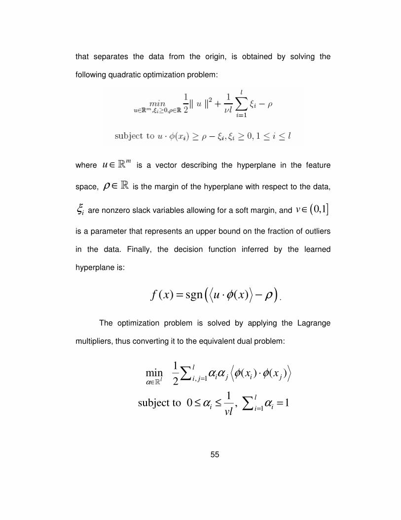
55
that separates the data from the origin, is obtained by solving the
following quadratic optimization problem:
where mu ∈� is a vector describing the hyperplane in the feature
space, ρ ∈� is the margin of the hyperplane with respect to the data,
iξ are nonzero slack variables allowing for a soft margin, and ( ]0,1v∈
is a parameter that represents an upper bound on the fraction of outliers
in the data. Finally, the decision function inferred by the learned
hyperplane is:
( )( ) sgn ( )f x u xφ ρ= ⋅ − .
The optimization problem is solved by applying the Lagrange
multipliers, thus converting it to the equivalent dual problem:
, 1
1
1 min ( ) ( )
2
1subject to 0 , 1
l
l
i j i ji j
l
i ii
x x
vl
αα α φ φ
α α
=∈
=
⋅
≤ ≤ =
∑
∑
�
56
with the hyperplane parameters given by 1
( )l
i iiu xα φ
==∑ .
In the context of the HGT detection problem the input space X
is the set of all possible nucleotide sequences whereas the feature space
m� comprises the selected set of compositional features of the
nucleotide sequences, i.e. the frequencies of all templates of size n. We
can use the learned decision function to induce a scoring measure GS of
genes belonging to a fixed genome G , where more atypical genes will
receive lower scores: ( ) ( )GS x u xφ= ⋅ .
When v=1, this last measure, GS , is proportional to the
covariance of the two vectors involved in the inner product. Additionally,
it is worth pointing out that for any feature map φ , the typicality measure
obtained from the solution of the one-class SVM optimization problem
and the covariance measure discussed in [81] will result in the same
relative ranking of genes with respect to typicality. This can be shown
with the help of the Lemma contained in Appendix A.
On the other hand, for values of 1v < , the optimal hyperplane
solution will have some coefficients iα assume a zero value; the genes
57
for which 0iα = will not contribute their compositional features ( )ixφ
to the computation of u .
From the above, we can give a natural interpretation to the
optimal hyperplane u as a generalized genome signature: when 1v =
the generalized signature is equivalent to the usual genome signature
which is computed as the mean of the gene signatures in the genome;
for 0 1v< ≤ the generalized signature will comprise only a subset of
special “signature genes.” This also constitutes a natural interpretation of
the parameter v for the problem that we try to solve here as an upper
bound on the fraction of gene transfers in the genome. In the next
section, we use this fact to estimate, via a series of experiments, the
optimal parameter v for any given genome so that the number of
recovered horizontal gene transfers is maximized. In the worst-case
scenario, the performance of the one-class SVM-based method can be
as good as the covariance-based method introduced in [81] (this is again
a direct sequence of the lemma in Appendix A), but in practice the
method we propose here achieves an average improvement of more
than 10% across the 123 archaea and bacterial genomes we have been
using as a reference.
58
3.3.1 Results
In this section, we present results for several datasets. First, we
carried out an experiment where artificial horizontal transfers have been
simulated across a collection of 123 archaeal and bacterial genomes. As
in [81], this simulation was carried out using a pool of more than 350,000
prokaryotic genes: in fact, we permitted all our genomes to exchange
genes while making sure that a given genome did not become a gene
donor for itself. The genes were randomly selected from the pool and
“inserted” in the i-th genome: the task at hand for each of the tested
methods was to recover as many as possible of these artificially inserted
genes. It is important to note here that, to the best of our knowledge, this
simulation as well as those mentioned in [81] are unique in that they are
carried out using donor sets comprising actual genes. The tested
methods included CAI, Wn and Wn-SVM. Moreover the set of donors is
the same as the set of acceptors, in other words we allowed our tested
genomes to exchange genes with one another in any conceivable
combination. As such, this is a realistic simulation of what happens
naturally (as it is currently understood).
In addition to the prokaryotic simulation and analysis, we present
an analysis of the human cytomegalovirus genome from the standpoint
59
of horizontal gene transfer and compare our results with existing
knowledge from the literature about genes of this virus.
3.3.1.1 Evaluation of Wn-SVM: prokaryotic donor and
prokaryotic hosts
For each of the 123 host organisms in turn, we conducted k=20
experiments of simulated transfers from the prokaryotic gene pool. The
latter, as we described above, contained the approximately 350,000
prokaryotic genes from the 123 genomes that we used as hosts – in
other words, the host genomes also played the role of donors. In each
experiment, the number of added genes was chosen to be a fixed
percentage of the number of genes in the host genome. The
“transferred” genes were selected from the donor pool at random and
with replacement. The simulated-transfer-experiments were carried out
for transfer percentages which ranged between 1% and 8% of the genes
in the host genome under consideration.
Given each genome and transfer percentage combination, each of
the tested methods had to recover as many of the artificially transferred
genes as possible, without using any a priori knowledge about the host
genome or the donor genes. The ideal method should recover each and
every one of the artificially added genes. However, our artificial insertions
60
compete for the top, putative-transfer positions with the horizontal gene
transfers which are already present in the genome under consideration.
Consequently, not all of the artificially inserted genes will occupy the top,
putative-transfer positions: the fraction of the artificially inserted genes
that a tested method manages to recover is referred to as the ‘hit ratio’ of
the method. We should point out that this situation poses no problem for
the purposes of simulation as it holds true for all of the tested methods,
and thus no method is favored at the expense of another.
In [81] we showed that the best performance was achieved for
templates of size w=8. We thus evaluated the W8 and W8-SVM
measures, and the Codon Adaptation Index (CAI). Table 2 summarizes
the methods under evaluation and their characteristics. Method m’s
overall performance across the N genomes under consideration is
defined as:
∑ ∑
=
=
G
k
i
GmirkN
mPerf
1
)(11
,
where )(Grm
i is the hit ratio obtained by the method m at the i-th
iteration of the experiment (with ki ≤≤1 )
61
For the one-class SVM method, we had the additional task of
estimating the parameter v which controls the fraction of genes that
contribute to the genome signature. For each genome and each given
percentage of added genes, we estimate the optimal value of the
parameter v so that the fraction of the artificially inserted genes
recovered by the SVM method is maximized. This estimation is done by
varying the value of v from 0 to 1 using a step of 0.1 and conducting
k=20 experiments for each value; performance was averaged over these
20 experiments and the value of v which maximized performance was
chosen as the optimal value for v . The highly optimized SVM package
LibSVM [82] was used to solve a total of 200 quadratic problems per
organism.
In Table 3 we list the overall performance of all methods for
different percentages of artificially-added genes. The entries of Table 3
are also shown in Figure 9 the form of a plot. Table 4 shows the
improvement that our new W8-SVM method achieves when compared to
the remaining methods: the improvement is shown both in absolute
percentage points (Part A of Table 4) and in terms of relative values
(Part B of Table 4) and represents the average across the 20
experiments that we carried out for each genome and artificial transfer
percentage. The amount of relative improvement that W8-SVM achieves
62
relative to method m is computed as the average increase in the number
of artificially-transferred genes that our method detects
W8/SVM1 1 ( ) ( )
( )
mm m
G mG G
Perf G Perf GRel Rel
N N Perf G
−= =∑ ∑
.
The latter is a measure of how many more horizontal transfers are
detected by W8-SVM. For example, in the experiments with 2% added
genes from the prokaryotic pool, the W8-SVM method discovered 10.6%
more artificial transfers than W8 and 33.6% more than CAI.
In Figure 10, we show a comparison between W8-SVM and W8
for each of the 123 genomes and for those experiments where we added
2% donor genes. As predicted theoretically, W8-SVM improves upon W8
essentially across all the genomes with which we experimented (but of
course is in no-case inferior to W8).
In Figure 11, we compare W8-SVM with the CAI method: we use
green solid bars to indicate the cases where W8-SVM outperforms CAI,
and red-colored bars for when CAI outperforms W8-SVM. The height of
each bar corresponds to the relative improvement mGRel achieved by our
method over CAI as an average over the 20 experiments and can be
either positive (green bars) or negative (red bars).
63
3.3.1.2 Evaluation of Wn-SVM: analysis of the human
cytomegalovirus genome
This experiment is of particular relevance given that we set out to
create a method that would be suitable for the analysis of large as well
as small genomes. As the genome of choice to analyze with our
Wn-SVM method, we selected the human cytomegalovirus, also known
as human herpesvirus 5 or HHV5. The reason for this particular choice
is due to our long standing interest in the cytomegalovirus in conjunction
with the fact that this is a virus that transmits very easily, knows no age
or geographic boundaries, has no seasonal dependencies and affects a
very large percentage of the population in modernized societies [83-85].
Figure 12 shows a map of the HHV5 genome marked by Wn-
SVM. The strain we worked with was the laboratory strain AD169 [86]. In
the absence of detailed knowledge as to the extent of horizontal
transfers into the cytomegalovirus genomes, we generated results for
three values of v, namely 1.0, 0.9 and 0.8, and reported a region as a
HGT if and only if it were marked as a HGT by Wn-SVM at all three
values of v. Supplementary Figure 1 shows the boundaries of the
evaluated genomic regions, the genes that overlap with each region, and
64
the similarity score assigned by Wn-SVM to each region. The forward
and reverse strands of the genome are treated separately and the genes
are shown on their respective strand. The evaluated regions were 300
nucleotides in length and consecutive regions overlapped by 200
nucleotides.
Several interesting results can be seen from. With some very
interesting exceptions that clearly demonstrate the capabilities of Wn-
SVM and which we will discuss next, effectively every single one of the
blocks of genes that are known to be conserved across the -
herpesvirinae is marked by Wn-SVM as native to the cytomegalovirus
genome, precisely as described in [87]. These blocks are: genes UL22
through UL33, UL45 through UL53, UL69 through UL72, UL75 through
UL80, UL85 through UL87, UL89 through UL105, UL112 through UL117,
and the TRL/IRL and TRS/IRS regions.
Although the above mentioned blocks of genes are marked as
herpesvirinae-specific, there are a few small regions within them which
are notably flagged as horizontally transferred. In particular, and as is
seen in
Figure 12, genes UL33, UL78, US12 and US21 are all reported by
Wn-SVM as horizontal transfer candidates. This is in fact a correct
result given that all four of these genes are G-protein coupled receptor
65
homologues and thus eukaryotic in origin. Also marked, in a piece-meal
fashion this time, is UL48, a virion protein that comprises several distinct,
non-contiguous domains (hence the piece-meal marking by Wn-SVM)
which are known to be characteristic of eukaryotes (see relevant entry
from Table 1 from [84]).
A few additional observations are warranted here as they further
demonstrate the new method’s capabilities and increased sensitivity.
First, we would like to point out that much of the genomic sequence
outside the gene blocks that are known to be conserved across
herpesvirinae have been marked as horizontal transfer candidates. This
is a very interesting result which does not contradict the current
knowledge about the cytomegalovirus and which suggests several new
avenues of investigation.
Another interesting region is the one that genes UL107, UL108
and (partially so) UL109 span. The region is marked as a horizontal
transfer candidate and we believe that it is correctly marked as non-
native. Indeed, our earlier analysis of this virus’ genome that we
described in [85] concluded that UL106 through UL111 are unlikely to
code for genes. This claim was verified by very recent work [87]: therein,
it was shown that the corresponding 5kbp region does code for a spliced
intron. More importantly, this region is not conserved in the murine
66
cytomegalovirus, a strain that is close to the analyzed AD169 strain.
Taken together these observations corroborate the Wn-SVM result about
the region in question.
Finally, and as can be seen from
Figure 12, the TRL6/7 and IRL6/7 regions are reported by Wn-
SVM to be non-native to the human cytomegalovirus. Although this last
statement may be in disagreement with the discussion presented in [87],
it bodes well with the more recent findings of [85] according to which
these two blocks are unlike the rest of the TRL and IRL regions and may
in fact be non-coding.
3.3.2 Conclusion
We introduced a new more sensitive method, Wn/SVM, that is
based on a one-class support vector machine (SVM). Wn/SVM utilizes
the generalized compositional features which we proposed in our earlier
work. Our current work represents a substantial point of departure in
that Wn-SVM relies on a distribution-free, one-class SVM method in
order to draw conclusions instead of defining an a priori model as in the
case of the covariance measure. For each gene in turn, the new method
computes a typicality score which is then used as a proxy for the
67
probability that the gene under consideration has been acquired through
a horizontal transfer event.
Additional very important methodological differences involve the
manner in which the genome’s compositional signature (“reference
signature”) is now computed. In the earlier, covariance-based method,
all genes of the genome at hand contributed equally to the genomic
signature. However, in the Wn-SVM method weights are chosen
optimally using the maximum margin criterion. As such, Wn-SVM
extends the notion of a compositional genomic signature by enforcing
genes to contribute their compositional features in a non-uniform fashion.
In fact, due to the constraints of the optimization problem, some genes
may end up not contributing at all to the genomic signature (they will be
assigned a weight of zero). Interestingly enough, preliminary analysis
shows that the informational genes are under-represented in this group
of signature genes, exactly as expected: these genes tend to have
atypical compositions and therefore should not be contributing to the
genomic signature.
It is also worth pointing out that from a mathematical standpoint,
our previous method, [81], can be viewed as a special case of the one-
class SVM category of approaches. It in fact corresponds to a fixed
parameter v=1, which is known to yield sub-optimal performance for
68
most classes of problems that have been solved using support vector
machines. Also, it should be pointed out that although the compositional
features used in this work comprised templates of size 8, further
performance improvements may be possible through the application of
Gaussian or polynomial kernels on the same features, or through the use
of especially-designed kernel functions that are applied directly on
sequences without any need to first extract the compositional features
(see chapter 8 of [32]).
With respect to evaluating the performance of Wn-SVM, we
carried out a comparative analysis of W8-SVM and W8 for the discovery
of horizontal gene transfers by inserting random, varying-size collections
of prokaryotic genes in each of 123 host genomes (archaea and
bacteria) and processing those artificially-created genomes with each
method in turn. Our findings clearly show that Wn-SVM offers significant
sensitivity improvements over Wn. We further validated Wn-SVM by
demonstrating its applicability to the analysis of smaller viral genomes,
an area of research that has to date remained unexplored from the
standpoint of horizontal gene transfer. As a case-study, we analyzed the
genome of the human cytomegalovirus (human herpesvirus 5) and
showed that we can successfully mark genomic regions as horizontally
transferred, in direct agreement with earlier independent studies. Finally,

69
we have made available Wn-SVM’s predictions for numerous, publicly
available archaeal, bacterial and viral genomes on the world-wide-web at
http://cbcsrv.watson.ibm.com/HGT_SVM/.
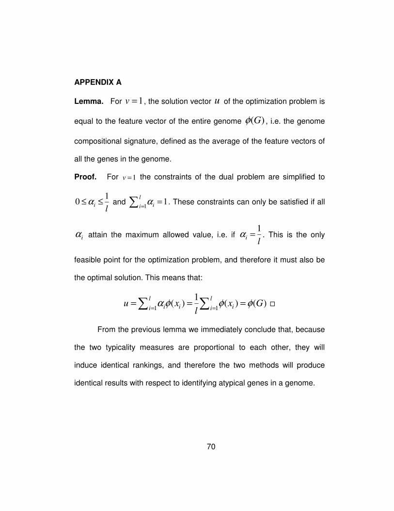
70
APPENDIX A
Lemma. For 1v = , the solution vector u of the optimization problem is
equal to the feature vector of the entire genome ( )Gφ , i.e. the genome
compositional signature, defined as the average of the feature vectors of
all the genes in the genome.
Proof. For 1v = the constraints of the dual problem are simplified to
10 i
lα≤ ≤ and
11
l
iiα
==∑ . These constraints can only be satisfied if all
iα attain the maximum allowed value, i.e. if 1
il
α = . This is the only
feasible point for the optimization problem, and therefore it must also be
the optimal solution. This means that:
1 1
1( ) ( ) ( )
l l
i i ii iu x x G
lα φ φ φ
= == = =∑ ∑ �
From the previous lemma we immediately conclude that, because
the two typicality measures are proportional to each other, they will
induce identical rankings, and therefore the two methods will produce
identical results with respect to identifying atypical genes in a genome.
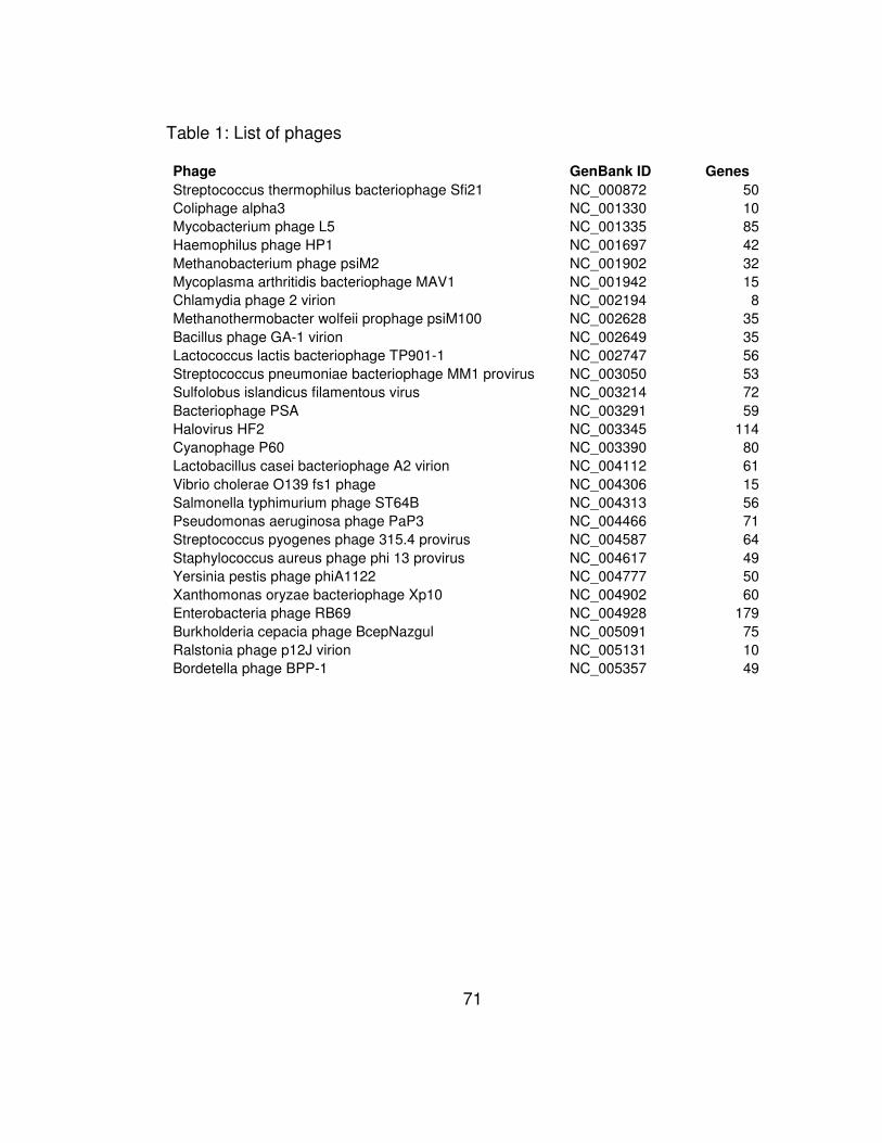
71
Table 1: List of phages
Phage GenBank ID Genes
Streptococcus thermophilus bacteriophage Sfi21 NC_000872 50
Coliphage alpha3 NC_001330 10
Mycobacterium phage L5 NC_001335 85
Haemophilus phage HP1 NC_001697 42
Methanobacterium phage psiM2 NC_001902 32
Mycoplasma arthritidis bacteriophage MAV1 NC_001942 15
Chlamydia phage 2 virion NC_002194 8
Methanothermobacter wolfeii prophage psiM100 NC_002628 35
Bacillus phage GA-1 virion NC_002649 35
Lactococcus lactis bacteriophage TP901-1 NC_002747 56
Streptococcus pneumoniae bacteriophage MM1 provirus NC_003050 53
Sulfolobus islandicus filamentous virus NC_003214 72
Bacteriophage PSA NC_003291 59
Halovirus HF2 NC_003345 114
Cyanophage P60 NC_003390 80
Lactobacillus casei bacteriophage A2 virion NC_004112 61
Vibrio cholerae O139 fs1 phage NC_004306 15
Salmonella typhimurium phage ST64B NC_004313 56
Pseudomonas aeruginosa phage PaP3 NC_004466 71
Streptococcus pyogenes phage 315.4 provirus NC_004587 64
Staphylococcus aureus phage phi 13 provirus NC_004617 49
Yersinia pestis phage phiA1122 NC_004777 50
Xanthomonas oryzae bacteriophage Xp10 NC_004902 60
Enterobacteria phage RB69 NC_004928 179
Burkholderia cepacia phage BcepNazgul NC_005091 75
Ralstonia phage p12J virion NC_005131 10
Bordetella phage BPP-1 NC_005357 49
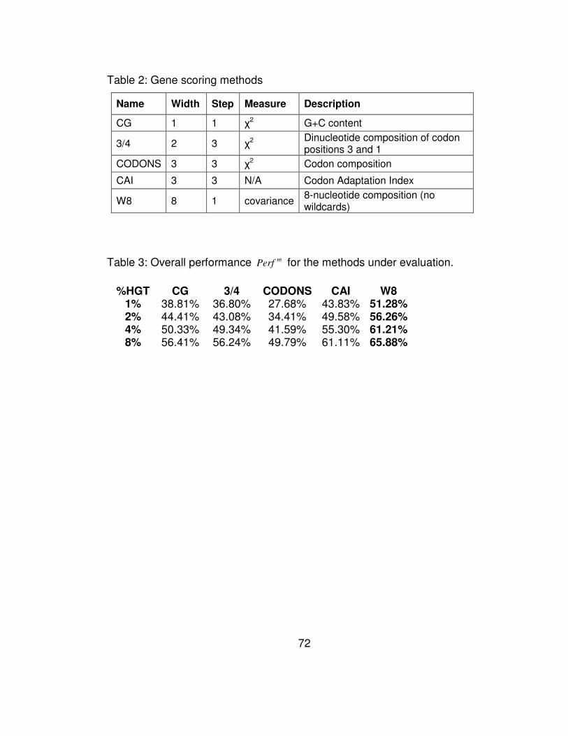
72
Table 2: Gene scoring methods
Name Width Step Measure Description
CG 1 1 χ2 G+C content
3/4 2 3 χ2 Dinucleotide composition of codon positions 3 and 1
CODONS 3 3 χ2 Codon composition
CAI 3 3 N/A Codon Adaptation Index
W8 8 1 covariance 8-nucleotide composition (no wildcards)
Table 3: Overall performance mPerf for the methods under evaluation.
%HGT CG 3/4 CODONS CAI W8 1% 38.81% 36.80% 27.68% 43.83% 51.28% 2% 44.41% 43.08% 34.41% 49.58% 56.26% 4% 50.33% 49.34% 41.59% 55.30% 61.21% 8% 56.41% 56.24% 49.79% 61.11% 65.88%
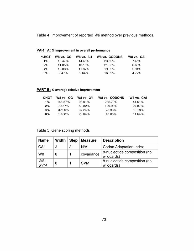
73
Table 4: Improvement of reported W8 method over previous methods.
PART A: % improvement in overall performance
PART B: % average relative improvement
%HGT W8 vs. CG W8 vs. 3/4 W8 vs. CODONS W8 vs. CAI
1% 146.57% 93.01% 232.79% 41.61%
2% 70.57% 59.82% 129.98% 27.87%
4% 32.90% 37.24% 78.96% 18.18%
8% 19.88% 22.04% 45.05% 11.64%
Table 5: Gene scoring methods
Name Width Step Measure Description
CAI 3 3 N/A Codon Adaptation Index
W8 8 1 covariance 8-nucleotide composition (no wildcards)
W8-SVM
8 1 SVM 8-nucleotide composition (no wildcards)
%HGT W8 vs. CG W8 vs. 3/4 W8 vs. CODONS W8 vs. CAI
1% 12.47% 14.48% 23.60% 7.45%
2% 11.85% 13.18% 21.85% 6.68%
4% 10.88% 11.87% 19.62% 5.91%
8% 9.47% 9.64% 16.09% 4.77%
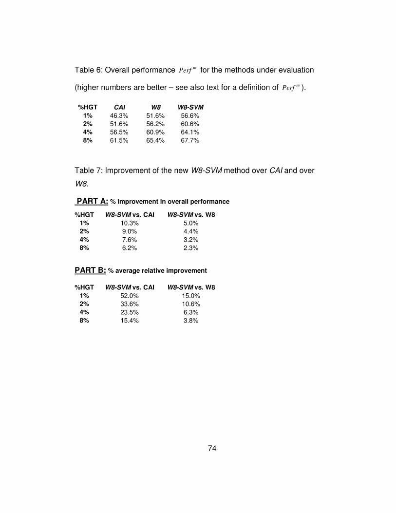
74
Table 6: Overall performance mPerf for the methods under evaluation
(higher numbers are better – see also text for a definition of mPerf ).
%HGT CAI W8 W8-SVM
1% 46.3% 51.6% 56.6%
2% 51.6% 56.2% 60.6%
4% 56.5% 60.9% 64.1%
8% 61.5% 65.4% 67.7%
Table 7: Improvement of the new W8-SVM method over CAI and over
W8.
PART A: % improvement in overall performance
PART B: % average relative improvement
%HGT W8-SVM vs. CAI W8-SVM vs. W8
1% 52.0% 15.0%
2% 33.6% 10.6%
4% 23.5% 6.3%
8% 15.4% 3.8%
%HGT W8-SVM vs. CAI W8-SVM vs. W8
1% 10.3% 5.0%
2% 9.0% 4.4%
4% 7.6% 3.2%
8% 6.2% 2.3%
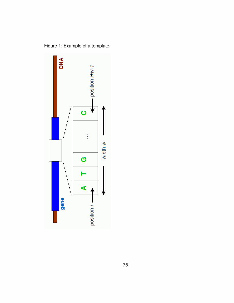
75
Figure 1: Example of a template.
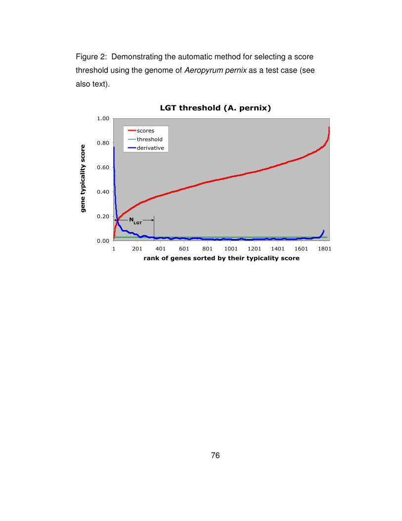
76
Figure 2: Demonstrating the automatic method for selecting a score
threshold using the genome of Aeropyrum pernix as a test case (see
also text).
LGT threshold (A. pernix)
0.00
0.20
0.40
0.60
0.80
1.00
1 201 401 601 801 1001 1201 1401 1601 1801
rank of genes sorted by their typicality score
gene typicality score
scores
threshold
derivative
NLGT
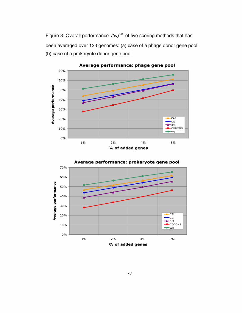
77
Figure 3: Overall performance m
Perf of five scoring methods that has
been averaged over 123 genomes: (a) case of a phage donor gene pool,
(b) case of a prokaryote donor gene pool.
Average performance: phage gene pool
0%
10%
20%
30%
40%
50%
60%
70%
1% 2% 4% 8%
% of added genes
Average performance
CAI
CG
3/4
CODONS
W8
Average performance: prokaryote gene pool
0%
10%
20%
30%
40%
50%
60%
70%
1% 2% 4% 8%
% of added genes
Average performance
CAI
CG
3/4
CODONS
W8
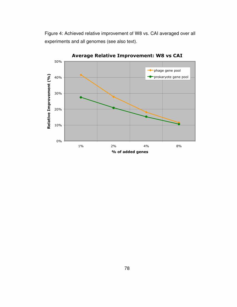
78
Figure 4: Achieved relative improvement of W8 vs. CAI averaged over all
experiments and all genomes (see also text).
Average Relative Improvement: W8 vs CAI
0%
10%
20%
30%
40%
50%
1% 2% 4% 8%
% of added genes
Relative Improvement (%)
phage gene pool
prokaryote gene pool
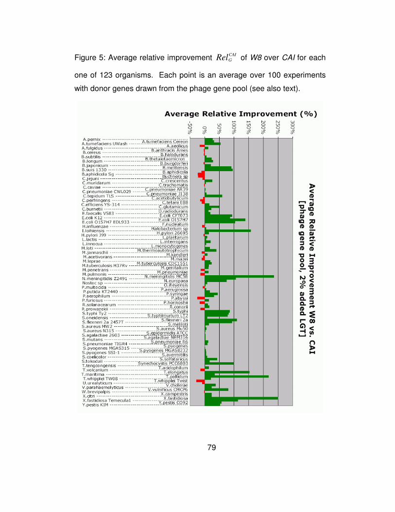
79
Figure 5: Average relative improvement CAI
GRel of W8 over CAI for each
one of 123 organisms. Each point is an average over 100 experiments
with donor genes drawn from the phage gene pool (see also text).
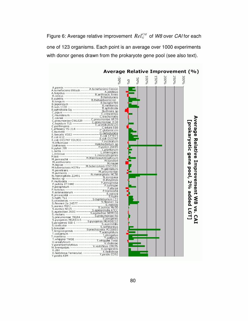
80
Figure 6: Average relative improvement CAI
GRel of W8 over CAI for each
one of 123 organisms. Each point is an average over 1000 experiments
with donor genes drawn from the prokaryote gene pool (see also text).
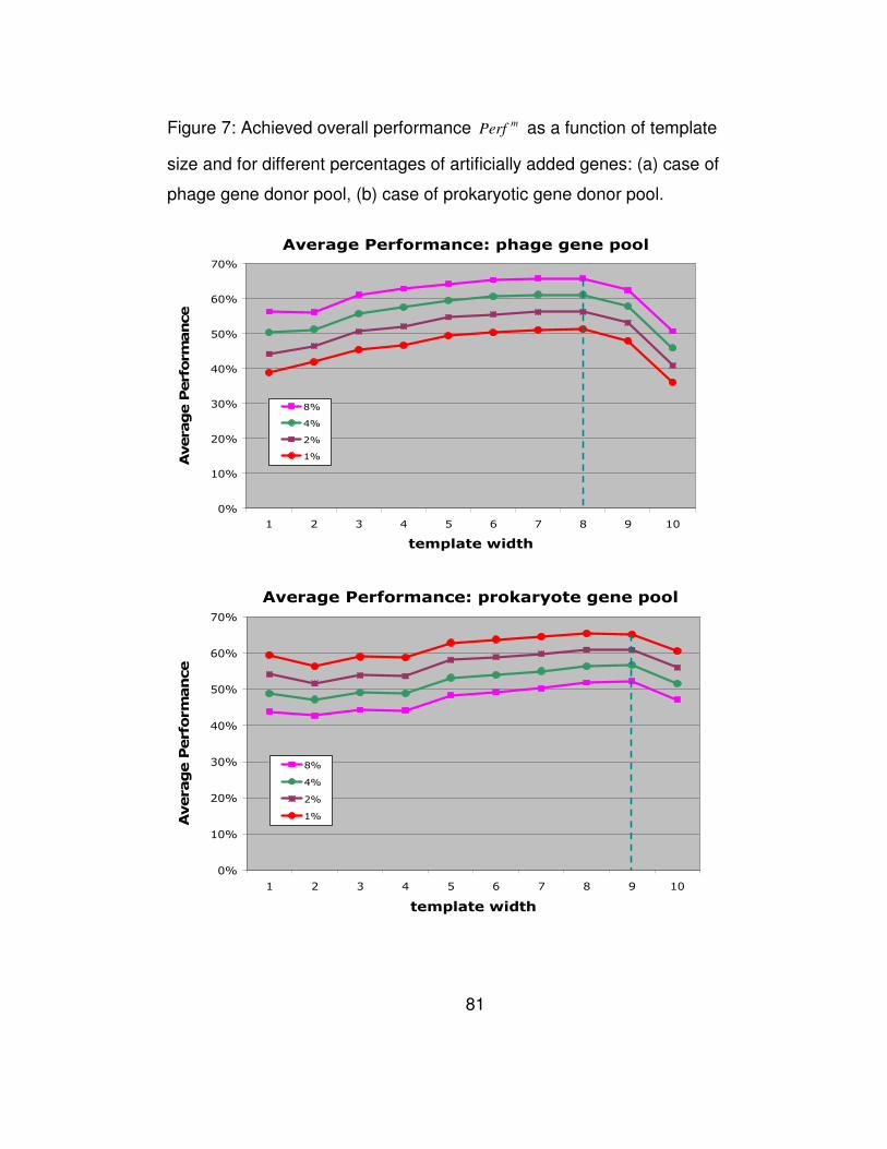
81
Figure 7: Achieved overall performance mPerf as a function of template
size and for different percentages of artificially added genes: (a) case of
phage gene donor pool, (b) case of prokaryotic gene donor pool.
Average Performance: phage gene pool
0%
10%
20%
30%
40%
50%
60%
70%
1 2 3 4 5 6 7 8 9 10
template width
Average Performance
8%
4%
2%
1%
Average Performance: prokaryote gene pool
0%
10%
20%
30%
40%
50%
60%
70%
1 2 3 4 5 6 7 8 9 10
template width
Average Performance
8%
4%
2%
1%
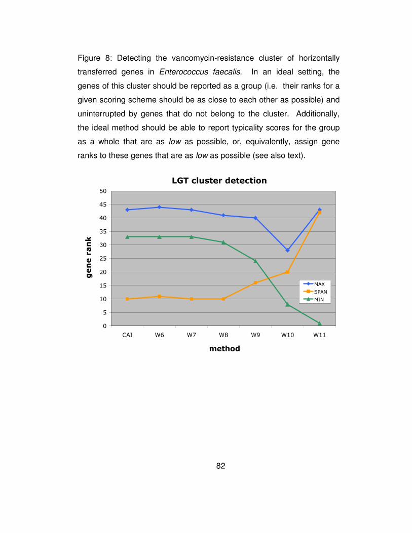
82
Figure 8: Detecting the vancomycin-resistance cluster of horizontally
transferred genes in Enterococcus faecalis. In an ideal setting, the
genes of this cluster should be reported as a group (i.e. their ranks for a
given scoring scheme should be as close to each other as possible) and
uninterrupted by genes that do not belong to the cluster. Additionally,
the ideal method should be able to report typicality scores for the group
as a whole that are as low as possible, or, equivalently, assign gene
ranks to these genes that are as low as possible (see also text).
LGT cluster detection
0
5
10
15
20
25
30
35
40
45
50
CAI W6 W7 W8 W9 W10 W11
method
gene rank
MAX
SPAN
MIN
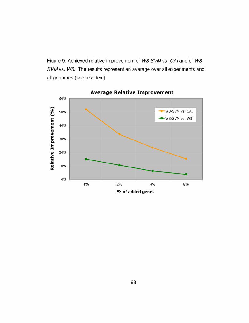
83
Figure 9: Achieved relative improvement of W8-SVM vs. CAI and of W8-
SVM vs. W8. The results represent an average over all experiments and
all genomes (see also text).
Average Relative Improvement
0%
10%
20%
30%
40%
50%
60%
1% 2% 4% 8%
% of added genes
Relative Improvement (%)
W8/SVM vs. CAI
W8/SVM vs. W8
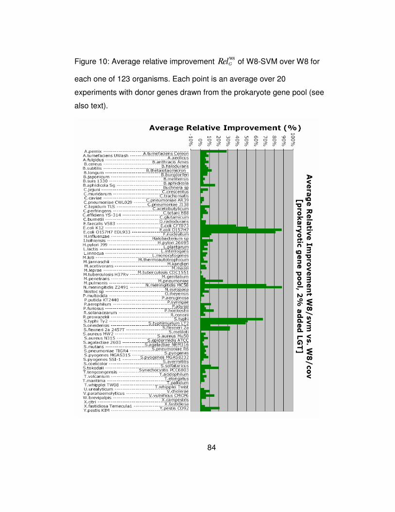
84
Figure 10: Average relative improvement W8
GRel of W8-SVM over W8 for
each one of 123 organisms. Each point is an average over 20
experiments with donor genes drawn from the prokaryote gene pool (see
also text).
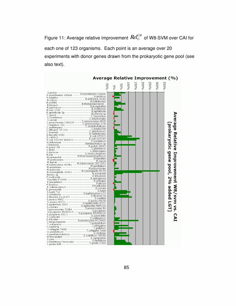
85
Figure 11: Average relative improvement CAI
GRel of W8-SVM over CAI for
each one of 123 organisms. Each point is an average over 20
experiments with donor genes drawn from the prokaryotic gene pool (see
also text).
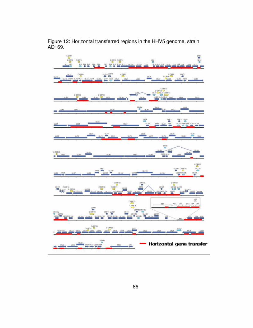
86
Figure 12: Horizontal transferred regions in the HHV5 genome, strain AD169.
87
4 Protein Localization
The computational prediction of a protein’s sub-cellular location
directly from the amino acid sequence is a well-known problem in
bioinformatics. Together with structural and functional protein annotation
methods, it is a valuable tool in high-throughput sequencing projects. In
this work, we introduce a new pattern-based method for the prediction of
a protein’s sub-cellular location that relies on the analysis of the
corresponding amino acid sequence. Our method uses a training set of
amino acid sequences to compute fixed-length and highly-significant,
variable-length amino acid patterns that it then uses in order to assign
unclassified proteins into one of twelve categories (i.e. sub-cellular
locations). Through a series of experiments, we demonstrate that the
new method can achieve improvements of more than 6% in total
accuracy and almost 13% in average sub-cellular location accuracy over

88
previous approaches. An implementation of the described method can
be accessed on the web at:
http://cbcsrv.watson.ibm.com/ProteinLocalization.
4.1 Related work
Intracellular protein sorting is responsible for maintaining the correct
structure and function of every cell within an organism. Organelles such
as the nucleus, Golgi, endoplasmic reticulum (ER) and plasma
membrane need to maintain a strict collection of resident proteins for
optimal function. The importance of protein sorting is highlighted only
when it breaks down and a disease state occurs [88, 89]. Protein
trafficking is a highly-complex procedure involving various forms of
cargo, carriers, destinations and routes. The entire process is highly
dynamic and characterized by the constant movement of proteins
throughout the cell.
Current hypotheses maintain that protein trafficking is dependent on
bulk flow movement through the cell in combination with active sorting
signals and retention signals which are present within proteins [90].
Most proteins are able to reach their destination by using one or more of
signals directing general bulk flow, active sorting or retention. For
89
example, a newly synthesized cadherin protein uses a N-terminal signal
sequence to enter the ER, bulk flow to transverse from the ER to the
Golgi and finally a basolateral sorting signal to reach the plasma
membrane. At the plasma membrane it can be either retained through
interaction with other cadherins, or undergo endocytosis through an as-
yet-undefined mechanism [91].
The myriad of trafficking steps undertaken by E-cadherin exemplify
the scale and difficulty of predicting a proteins sub-cellular localization.
Experimental validation of the sub-cellular localization of an individual
protein is currently a slow and labor-intensive process. Computational
methods that can help speed-up the elucidation of the underlying
sequence signals are thus very important.
Predicting sub-cellular localization is a well known problem in
computational biology and several methods have been proposed to date
that address this task. We refer the interested reader to several review
articles which have already covered this subject [92-94] rather
extensively.
The localization prediction methods can be broken down into two
major categories. The first category utilizes protein sorting and retention
signals to predict protein localization. Traditionally, the focus has been
on predicting secreted and plasma membrane proteins due to their
90
importance for multicellular organisms. Some recent additions to this
class of methods include the ones described in [95-102]. An important
limitation of these methods is that they rely on the knowledge of such
signals: unfortunately, many of the signals remain unknown.
The second category of methods predict the location of proteins by
relying on the observation that global sequence features, such as amino
acid composition, are specific to sub-cellular location [103]. Numerous
tools following this approach have been developed in the recent years,
the most prominent of which are described in [104-111]. Hybrid methods
have also been reported in the literature [112, 113].
4.2 Overview of unsupervised pattern discovery
Our method is based on the use of a collection of amino acid patterns
that are discovered in an automated manner and cover the sequence
space of the training set under consideration. Such signals have been
shown to capture functional and structural signals [27-29].
Typically, an unsupervised pattern discovery tool takes a set D of
protein sequences as input and automatically discovers a
comprehensive set of patterns that appear many times in different
subsets of sequences. For the work described below, we have used the
Teiresias pattern discovery algorithm [10, 114]; the algorithm can
91
provably find all patterns p in the input set D that satisfy the following
properties:
(1) each p is composed of either literal characters, i.e. individual
amino acids, or classes of amino acids (designated by brackets),
possibly separated by a number of wild-cards characters (“dots”); a
wild-card indicates that the corresponding position can be occupied
by any amino acid.
(2) each p comprises at least L literal characters (or equivalence
classes) in any span of W L≥ positions. Then the pattern p is
considered to be an ,L W
pattern. For example, the pattern
A.C.[115]..L is a <2,4> pattern, whereas patterns A…C.[FY]..L,
A.C...[FY]..L and A.C.[FY]…L are not.
(3) each p occurs at least K times in the set D. K is referred to as
the “support” of pattern p.
Teiresias works in two phases which are termed scanning and
convolution. Scanning is performed in order to discover all <L,W>
patterns with length at most W (“seed patterns”). These seed patterns
are combined during convolution to form progressively longer patterns.
The extension process is guided by the contents of the processed
dataset and thus terminates naturally – the algorithm imposes no upper
bounds on the length of the discovered patterns.
92
4.3 Method A: fixed-length patterns
We first attempt to build a classifier for predicting protein sub-cellular
locations using only the seed patterns that are generated by the
scanning phase of Teiresias. The key idea is to explore the use of
higher-order amino acid patterns (cf. the amino acid pairs used in [106])
in an effort to improve accuracy while at the same time discover a simple
one-classifier model to perform the task. This bypasses the need for
elaborate voting schemes that are necessary when multiple classifier
methods are used.
The discovery step generated a total of 5,433,264 patterns that
belong to one of the four different categories shown here:
• L=1 and W=1 with chemical equivalences: this category
comprises 27 patterns, one pattern for each of the 20 amino acids
plus one for each of the 7 chemical equivalence classes shown in
Table 8. It is also referred to as single amino acid composition.
• L=2 and W=2 with chemical equivalences: this class comprises a
total of 272 = 729 patterns, and is also known as composition of
amino acid pairs.
• L=3 and W=5 with chemical equivalences: this category
comprises all patterns containing exactly 3 letters (amino acids, or
93
equivalence classes of amino acids) possibly separated by at
most two wildcards, a total of 6·273 = 118,098.
• L=4 and W=6 with chemical equivalences: this category
comprises all patterns containing exactly 4 letters (amino acids, or
equivalence classes of amino acids) possibly separated by a total
of at most two wildcards, a total of 10·274 = 5,314,410.
In Table 9 we show several examples of patterns from each category.
These four types of patterns are then used to decompose the input
sequences: each protein is effectively converted into a feature vector
with each feature corresponding to one of the discovered patterns – the
value of the feature is equal to the number of times the pattern is found
in the protein sequence. These feature values are subsequently
normalized per unit length, so as to remove the bias which would favor
longer proteins. Also, given that shorter patterns/features are expected to
occur much more frequently than longer ones, we linearly scale the
feature values across proteins of each feature separately, so that they
range from 0 to 1: this removes the bias towards more frequent patterns
and is a necessary step (otherwise, more frequent patterns would have
been treated as more predictive that less frequent ones). Intuitively,
there must exist longer patterns which, despite occurring only once in
some sequences, they can actually be used to predict protein localization
94
much more accurately than the frequency of single amino acids because
they turn out to be specific to a given sub-cellular location.
After the preprocessing of the train and test feature vectors is
complete, we train a all-against-all multi-class SVM classifier [116, 117]
using an RBF kernel6 and classify the test vectors according to the model
obtained from the training phase. The highly optimized SVM package
LibSVM by Chang and Lin was used to train the SVM classifier and do
the final testing: see http://www.csie.ntu.edu.tw/~cjlin/libsvm for the code
and reference manuals for LibSVM. The training and testing process are
summarized in Figure 13.
It is worth mentioning that for a classification problem that is
characterized by millions of features, feature selection becomes an
important preprocessing step. As advocated by LibSVM developers
[118], we apply multi-class Fisher scoring [119] to evaluate the
importance of individual features. We found that selecting 25% of the
top scoring features boosts classification accuracy by 2-3%, while
significantly reducing classifier training and testing times.
6 ( )2
( , ) expK x y x yγ= − − , where x and y are vectors of the same size and
γ>0.
95
4.4 Method B: variable-length patterns
The following observations highlight the importance of discovering
variable-size patterns in the input set (training set).
• patterns that are allowed to grow in length in an unrestricted
manner will be as specific as possible for the given input dataset
• long patterns can be highly significant even if they appear few
times in the dataset
• highly-significant, variable-length patterns can help identify
important local similarities among sequences which are destined
for the same sub-cellular location; on the other hand,
computations of similarities among full-length sequences can lead
to artificially high (or low) values since they ignore the small-by-
comparison part of the sequence which is relevant for the
classification task at hand.
The training and testing process for Method B is summarized in
Figure 14. In the first step, unsupervised pattern discovery is performed
using both the scanning and the convolution phases of Teiresias in order
to extract all, maximal in composition and length patterns in the training
set. The parameters we used for this step were L=4 and W=6 with
minimum support set to K=2 – no amino acid equivalences were taken
96
into account. In general, the total number of discovered patterns can be
very high. Clearly, this number can be affected by the choice of
parameters and the use of amino acid equivalences (e.g. chemical,
structural etc.). As one would intuitively expect, a larger pattern
collection could potentially increase the final classification performance.
However, in the presence of more patterns, the training and classification
tasks would become harder to manage given that the computational
resources in terms of memory, disk storage and processing power are
finite.
During the second step, we compute z-scores for each discovered
pattern as a function of its expected probability and its support in the
database. Formally, the z-score zp of a pattern p is computed using the
following formula:
( )
( ) ( )( )ppD
pDN ppz
Pr1Pr
Pr
−⋅⋅
⋅−=
where Np is the observed number of occurrences of the pattern in the
given dataset, D is the size of the dataset (total number of amino acids),
and Pr(p) is the expected probability of the pattern given the observed
probabilities of single amino acids assuming iid. Patterns that have z-
scores lower than a threshold θ are discarded.
97
The third step ensures that, among the highly-significant patterns,
only those which give rise to the same sub-cellular location are kept: in
other words, we keep only the patterns that are found in protein
sequences of the same sub-cellular location (zero-entropy). We note
here that since this is done using the training set only there is no
guarantee that the same will hold true in the test set. However, this
“guilty by association” approach has been time-honored and is very
typical for this kind of methods: intuitively, we do expect this to be the
case most of the time.
With the completion of the third step, we now have a set of highly-
significant patterns each one of which is associated with a specific sub-
cellular location. We use these pattern sets as predicates that can
predict the eventual sub-cellular location of the test sequences. Since
there is no guarantee that these patterns will appear in a test sequence
unchanged, we introduce what we refer to as a “pattern matching score”
between a pattern and a protein sequence: this score is defined as the
maximum fraction over all possible ungapped alignments of the total
number of matched amino acids in the pattern/protein alignment divided
by the total number of matched and unmatched amino acids – obviously,
this score ranges between 0 and 1 inclusive.
98
We are now ready to assign predictions to our test sequences. This
is simply done by finding, for any given test sequence, the pattern with
the highest z-score which aligns best with the test sequence (i.e. leads to
the highest matching score). If the matching score is greater than or
equal to a threshold α, then the test sequence is assigned to the location
associated with the matching pattern, otherwise it remains unassigned
(inability to predict with confidence). In other words, we try each pattern
in turn, in order from the highest to the lowest z-score: when a pattern is
found whose matching score is not lower than α, we stop and assign the
test sequence to the sub-cellular location of the pattern at hand. Clearly,
more elaborate schemes could be applied, but such an endeavor is
beyond the scope of this work; our goal is to demonstrate that variable-
length patterns can in fact be used effectively to improve prediction
accuracy. In the Results section we explain how to use Method B in
conjunction with Method A in order to deal with the test sequences that
are left unclassified by Method B.
4.5 Results
4.5.1 Method A: fixed-length patterns
Despite the fact that a lot of research has been done on
computationally predicting protein sub-cellular locations, the area still
99
lacks universally accepted reference datasets and performance
measures. We thus chose to work with the dataset introduced in [106]
which includes a large number of proteins classified into 12 sub-cellular
location (i.e. categories). The location-specific datasets are derived from
eukaryotic entries of Swiss-Prot database release 39.0 based on the
content of SUB-CELLULAR LOCATION section of CC (comment) lines:
the 12 sub-cellular locations that are covered include chloroplast,
cytoplasm, cytoskeleton, endoplasmic reticulum (ER), Golgi apparatus,
lysosome, mitochondria, nucleus, peroxisome, plasma membrane, and
vacuole. The datasets are located at http://web.kuicr.kyoto-
u.ac.jp/~park/Seqdata/. The number of entries in each category is
indicated in the first column of Table 10.
We estimate the prediction performance of our method using a 5-fold
cross-validation test as in [106]. The idea of the test is to split the
dataset into five approximately equal subsets. One subset is used as a
test set; the remaining four subsets are combined together into a training
set. This process is repeated five times so that each protein sequence is
evaluated once. The final performance is measured on the five test sets
and is defined separately for each sub-cellular location i as i i iP T n= ,
where iT is the number of sequences correctly ascribed to the i-th
100
category (a.k.a. true positives) and in is the total number of sequences
in this category. This last measure is often referred to as sensitivity. In
addition, we define two cumulative, location-independent measures. The
first one, location accuracy, is an average of i
P over all K locations and is
defined as follows:
1
K
iiLP P K
==∑ .
The second measure, total accuracy, is the fraction of correct
predictions for the total of N sequences in the dataset and is defined as
follows:
1
K
iiTP T N
==∑ .
The two cumulative measures are complementary: TP tracks
performance mainly in categories with large numbers of sequences. On
the contrary, LP treats each category equally regardless of the
category’s size.
We set up an optimization grid in order to determine the optimal
parameters β, c and γ of our SVM classifier: β is the percentage of top
scoring features selected for training, c is used to control the complexity
of the learned hyperplane, and, γ is a parameter of the RBF kernel. As
shown in Figure 15, the test accuracy is computed for each parameter
101
triplet (c,γ,β) using the 5-fold cross-validation process. Using this
process, we determined that the maximum test accuracy was achieved
when β=25%, c=64 and γ=0.0001, and the resulting value for the total
accuracy of our SVM classifier was 82.4%. This represents a very
significant performance improvement over PLOC whose total accuracy is
78.2%.
This performance improvement is particularly notable if one considers
the following:
a) it is obtained using a single classifier (vs. 5 classifiers used by
PLOC);
b) there is a single value for the parameter γ of the RBF kernel (vs.
use of a mixture of two different γ values by PLOC); and, most
importantly,
c) our approach obviates the need for the use of a voting scheme that
combines the results from multiple classifiers.
Analogously, our achieved location accuracy performance is
62.1% which again represents a considerable improvement over PLOC’s
performance of 57.9%. Table 10 details the results of our method for
each category separately.
102
4.5.2 Method B: variable-length patterns
Figure 16 highlights the tradeoff between accuracy and coverage at
various z-score threshold levels when Method B is used alone: as the
threshold for pattern selection increases the number of sequences in the
test set that will be covered by those patterns decreases, but the
prediction accuracy does increase as a result. For example, at z-score
threshold logθ=20, only 63% of the 7579 proteins are classified but the
classification accuracy reaches the impressive level of 93.5%; however,
if we attempt to cover more proteins by lowering the threshold to
logθ=15, although almost all proteins are covered (96%), the
classification accuracy drops sharply.
These findings suggested that instead of trying to cover all
sequences using the individual patterns of Method B, a hybrid method
that combined the best characteristics from Method A and Method B
would be a better choice.
4.5.3 Hybrid Method B/A: fixed- and variable-length patterns
The hybrid scheme that we advocate works as follows. We first use
Method B to classify a test sequence. If none of the patterns that
Method B has at its disposal have instances in the sequence at hand,
then Method A is brought to bear.

103
The same training and testing approach used for Method A was
applied in order to evaluate the hybrid Method B/A. A grid search was set
up in order to determine the optimal z-score threshold θ and the pattern
matching cutoff α for our Method B classifier, while, for Method A, we
simply used the optimal parameters obtained from the previous
optimization of Method A alone. The optimization process for determining
the optimal parameters of α and θ is summarized in Figure 17. Ideally,
we would have attempted a joint optimization over all 5 parameters of the
two methods, which would probably have increased performance even
further. However, this optimization over 5 parameters would have
required a tremendous amount of computational resources.
This hybrid scheme works very well as can be seen from the results
shown in Table 10. The hybrid Method B/A approach exhibits markedly
better total (=84.4%) and location (=70.8%) prediction accuracies when
compared to the corresponding PLOC values (78.2% and 57.9%
respectively). These numbers reflect an improvement of 6.2% and 12.9%
respectively. This is especially important for the location accuracy as it
implies that better predictions can now be made for the under-
represented categories. Indeed, we achieve an almost 3–fold
improvement for the “Golgi apparatus” category and a 2–fold
improvement for the “peroxisome” and “vacuole” categories when
104
compared to PLOC. Analogous performance improvements are achieved
for all remaining location categories as can be seen in Figure 18.
4.6 Conclusion
We have presented a new method that allows to confidently predict
sub-cellular protein locations. It is based on the unsupervised discovery
of fixed-length as well as variable-length patterns. Our method results in
a significantly-improved ability to predict a protein’s eventual location
directly from amino acid sequence. When compared with the state-of-
the-art amino-acid-composition-based tool PLOC, we demonstrate
improvements of total accuracy by 6.2% and of location accuracy by
12.9% respectively.
Despite significant computational advances over the years, the
problem of sub-cellular protein localization is still far from solved for
eukaryotic organisms. And, even though we have demonstrated that our
method achieves significant prediction gains, we believe that it is only
prudent for practitioners to use the output from all available prediction
tools before drawing any conclusions.
Our future work will concentrate on the analysis of factors which limit
the performance of the proposed method. In this regard, one important

105
improvement, we believe, is likely to result from the use of
organism-specific datasets. A significantly harder variation of this
problem would require that one address the case of proteins with
multiple locations and that one predict all intermediate such locations.
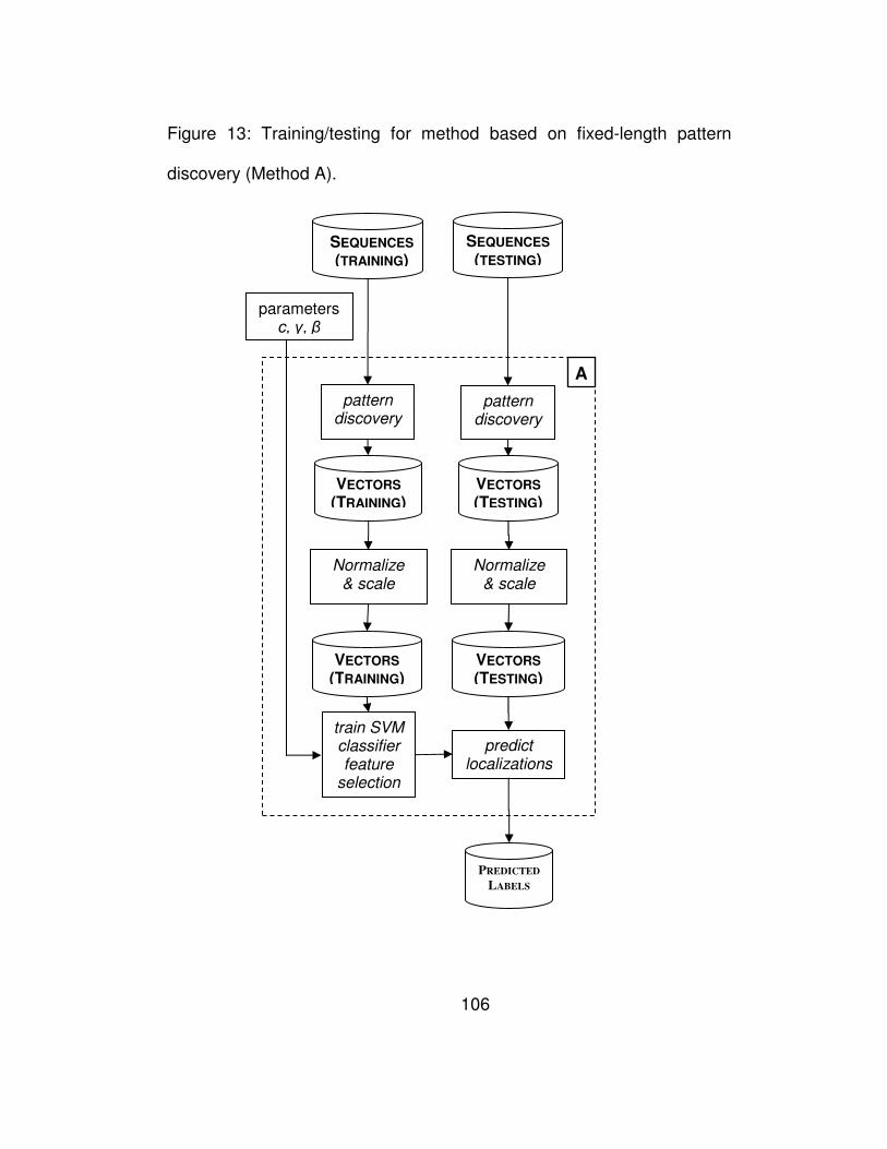
106
Figure 13: Training/testing for method based on fixed-length pattern
discovery (Method A).
SEQUENCES (TESTING)
VECTORS (TRAINING)
VECTORS (TESTING)
SEQUENCES
(TRAINING)
pattern discovery
pattern discovery
VECTORS (TRAINING)
VECTORS (TESTING)
train SVM classifier feature
selection
predict localizations
PREDICTED
LABELS
A
parameters c, γ, β
Normalize & scale
Normalize & scale
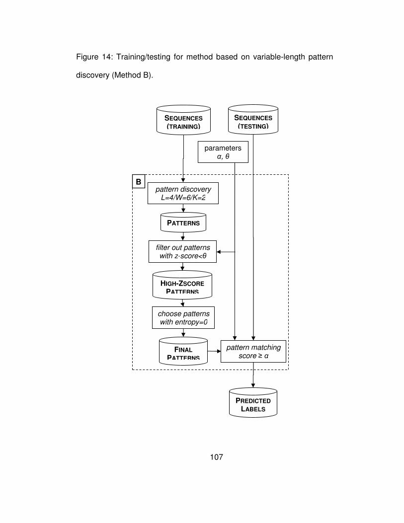
107
Figure 14: Training/testing for method based on variable-length pattern
discovery (Method B).
SEQUENCES (TESTING)
PATTERNS
SEQUENCES
(TRAINING)
pattern discovery L=4/W=6/K=2
HIGH-ZSCORE PATTERNS
filter out patterns with z-score<θ
FINAL PATTERNS
choose patterns with entropy=0
pattern matching score ≥ α
PREDICTED LABELS
B
parameters α, θ
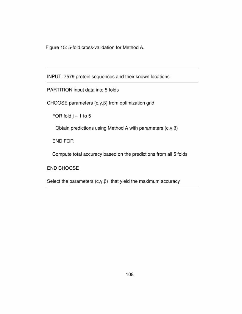
108
Figure 15: 5-fold cross-validation for Method A.
INPUT: 7579 protein sequences and their known locations
PARTITION input data into 5 folds
CHOOSE parameters (c,γ,β) from optimization grid
FOR fold j = 1 to 5
Obtain predictions using Method A with parameters (c,γ,β)
END FOR
Compute total accuracy based on the predictions from all 5 folds
END CHOOSE
Select the parameters (c,γ,β) that yield the maximum accuracy
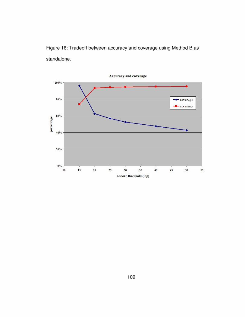
109
Figure 16: Tradeoff between accuracy and coverage using Method B as
standalone.
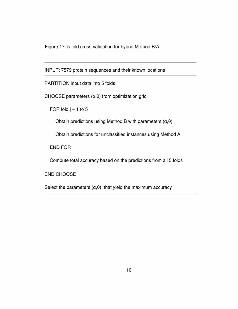
110
Figure 17: 5-fold cross-validation for hybrid Method B/A.
INPUT: 7579 protein sequences and their known locations
PARTITION input data into 5 folds
CHOOSE parameters (α,θ) from optimization grid
FOR fold j = 1 to 5
Obtain predictions using Method B with parameters (α,θ)
Obtain predictions for unclassified instances using Method A
END FOR
Compute total accuracy based on the predictions from all 5 folds
END CHOOSE
Select the parameters (α,θ) that yield the maximum accuracy
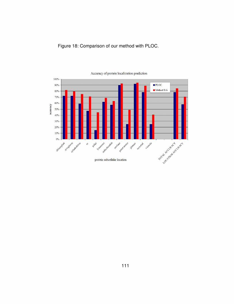
111
Figure 18: Comparison of our method with PLOC.
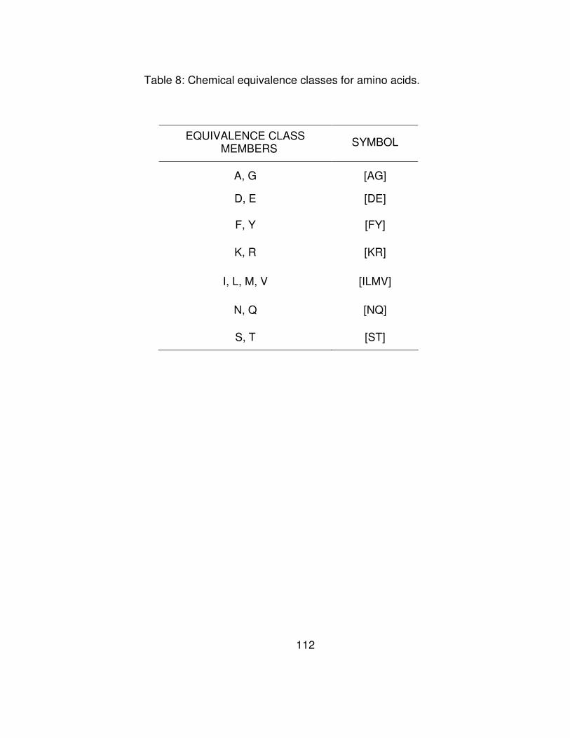
112
Table 8: Chemical equivalence classes for amino acids.
EQUIVALENCE CLASS MEMBERS
SYMBOL
A, G [AG]
D, E [DE]
F, Y [FY]
K, R [KR]
I, L, M, V [ILMV]
N, Q [NQ]
S, T [ST]
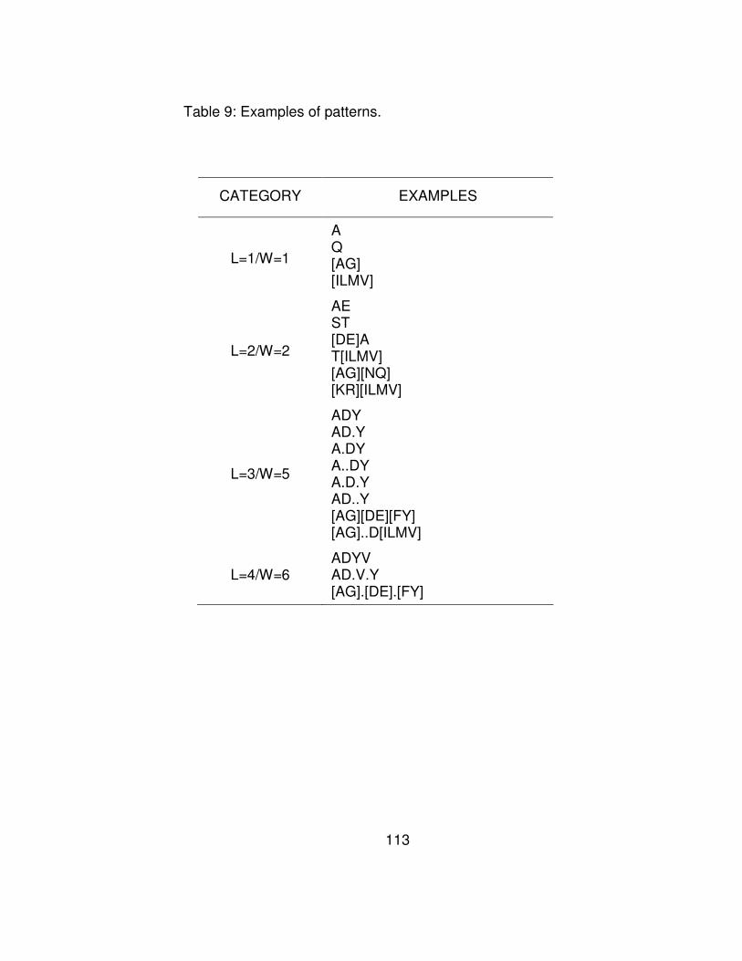
113
Table 9: Examples of patterns.
CATEGORY EXAMPLES
L=1/W=1
A Q [AG] [ILMV]
L=2/W=2
AE ST [DE]A T[ILMV] [AG][NQ] [KR][ILMV]
L=3/W=5
ADY AD.Y A.DY A..DY A.D.Y AD..Y [AG][DE][FY] [AG]..D[ILMV]
L=4/W=6 ADYV AD.V.Y [AG].[DE].[FY]
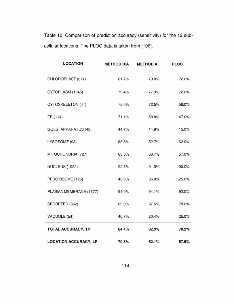
114
Table 10: Comparison of prediction accuracy (sensitivity) for the 12 sub-
cellular locations. The PLOC data is taken from [106].
LOCATION METHOD B/A METHOD A PLOC
CHLOROPLAST (671) 81.7% 79.0% 72.0%
CYTOPLASM (1245) 79.4% 77.9% 72.0%
CYTOSKELETON (41) 75.0% 72.5% 59.0%
ER (114) 71.1% 58.8% 47.0%
GOLGI APPARATUS (48) 44.7% 14.9% 15.0%
LYSOSOME (93) 68.8% 52.7% 62.0%
MITOCHONDRIA (727) 63.5% 60.7% 57.0%
NUCLEUS (1932) 92.5% 91.3% 90.0%
PEROXISOME (125) 48.8% 36.0% 25.0%
PLASMA MEMBRANE (1677) 94.0% 94.1% 92.0%
SECRETED (862) 89.0% 87.6% 78.0%
VACUOLE (54) 40.7% 20.4% 25.0%
TOTAL ACCURACY, TP 84.4% 82.3% 78.2%
LOCATION ACCURACY, LP 70.8% 62.1% 57.9%
115
5 Transcription factor binding site prediction
The discovery of transcription factor-binding site pairs has
applications ranging from medicine to nanotechnology. Microarray data
provides a promising base from which to infer such pairs, but pose two
important challenges: (a) microarray measurements are often noisy
making it difficult to obtain reliable correlation measurements; (b)
transcription often depends on multiple transcription factor-binding site
pairings, so simple correlation is insufficiently powerful to discover
individual pairings. In this work, we propose a novel method for the
discovery of candidate binding sites for transcription factors via the
computation of bi-clusters that measure the degree of correlation in
specific experimental conditions between a transcription factor and a set
of genes containing a potential binding site. We demonstrate that our bi-
cluster based method performs better than a method that is simply based
on pair-wise correlations between the transcription factor and the genes
containing the binding site. Moreover, we demonstrate that the number
116
of ways different sets of genes containing a binding site for a
transcription factor are co-expressed with the transcription factor, i.e. the
total number of bi-clusters, is higher than the number of bi-clusters found
in a set of genes that contain a motif different that the actual binding site,
a result that is in accordance with the notion of combinatorial regulation.
5.1 Related work
Motifs are short DNA sequences present in the upstream regions
of genes that play some kind of regulatory role in protein expression.
Motif finding in unaligned DNA sequences is therefore a fundamental
problem in computational biology, because it can potentially unveil the
regulatory signals that control the processes of activating and repressing
genes.
The most popular methods for motif finding depend on the
probabilistic modeling (profile) of the motifs, usually with variations of
Position-Specific Scoring Matrices (PSSMs) obtained as a summary of
multiple motif alignments. Different searching methods have been used
resulting in different tools: the Gibbs Motif Sampler (Lawrence et al. 1993
[2], Neuwald et al. 1995 [3]), based on Gibbs sampling, MEME (Bailey
and Elkan 1995 [4]), based on multiple runs of the Expectation
117
Maximization algorithm, AlignACE (Roth et al. 1998 [5]), based on
information content maximization, PSI-BLAST (Altschul et al. 1997 [6]),
based on iterative refinement of initial sequence alignments,
CONSENSUS (Hertz and Stormo 1999 [7]), and other [8, 9, 120-122].
These methods aim at discovering the highest scoring signals and are
not necessarily suitable for cases where a pair of monad signals, i.e. a
dyad signal, is sought, since the members of the dyad signal would be
statistically significant as a pair but not necessarily as individuals. In fact,
many of the actual regulatory signals are composite patterns, i.e. groups
of monad patterns [123].
Profile-based methods have been extended to detect dyad signals
in GuhaThakurta and Stormo (2001) [124] and Liu et al. (2001) [125], but
are based on approximations and therefore they cannot guarantee that
all signals will be discovered. Exhaustive enumeration using suffix trees
is performed in the dyad pattern search algorithm of Marsan and Sagot
(2000) [126]. Based on the observation that many regulatory sites
consist of a pair of highly conserved trinucleotides separated by a fixed
number of unconserved nucleotides, a method called dyad analysis was
introduced by van Helden et al. (2000) [127], which reports dyads
conforming to the pattern described above and satisfying some notion of
statistical significance. Finally, MITRA [128] is designed to discover
118
composite patterns that occur with mismatches. It is based on the
pairwise similarity information introduced in the WINNOWER algorithm
[121], and borrows the trie structure for data indexing used in the Speller
algorithm [129].
In order to provide a complete picture of the regulatory
mechanisms that determine gene expression in the cell, the complete
map of interactions among regulatory elements (e.g. cis-elements),
regulating proteins (e.g. transcription factors) and regulated genes must
be composed.
An enormous research effort is being devoted to uncovering this
interaction map. Clearly, upstream regions, which are used as input in
the motif discovering methods presented in the previous section, must be
combined with other types of data in order for this to be possible.
Usually, the additional data comes in the form gene expression data
obtained from microarray experiments. Models for combining the two
types of data can be found in Zhang (1999) [130], Vilo and Kivinen
(2001) [131], Ohler and Niemann (2001) [132], and Werner (2001) [133].
Broadly speaking, the huge variety of computational methods for
discovering regulatory networks can be distinguished in three categories.
In the first category, we find methods whose starting point is the
discovery of groups (or clusters) of potentially co-regulated genes in
119
terms of their expression levels across multiple experiments. Given a
group of potentially co-regulated genes, and under the assumption that
there is a causal link between the gene upstream region and the
observed co-expression, they attempt to identify cis-elements by looking
for overrepresented motifs in the upstream regions of the genes in the
cluster (Brazma et al. 1998 [134], Roth et al. 1998 [5], Tavazoie et al.
1999 [135], Sinha and Tompa 2000 [136], Liu et al. 2001 [125]).
Methods of the second category approach the problem from the
opposite direction. First, they perform some kind of unsupervised pattern
discovery on the upstream sequences, which can either be exhaustive or
may utilize one of the methods presented in the previous section.
Another option is to use only experimentally validated binding sites,
using one of the available databases, such as TRANSFAC (Wingender
et al., 2001 [137]). Then, a model for gene expression is built comprising
the genes and the discovered motifs, the model is fitted to the available
data, and finally it is evaluated in terms of whether it actually uncovers
parts of the underlying biological mechanisms involved. A wide variety of
models have been applied, such as Bayesian Networks in Barash and
Friedman (2001) [138], and Probabilistic Relational Models in Segal et al.
(2001, 2002, 2003) [139-141]. Birnbaum et al. (2001) [142] use a linear
model to describe the relationship between transcription factors and
120
motifs, defining the aggregate motif expression as the sum of
expressions of genes containing the motif in their upstream region, and
correlating it to the expression of known transcription factors.
Bussemaker et al. (2001) [143] models gene expression with a weighted
linear combination of the number of occurrences of each motif in the
gene upstream region. The method presented in Pilpel et al. (2001)
[144], seeks significant combinatorial interactions between pairs of
putative transcription factors. Other methods for identifying both cis-
elements and groups of co-expressed genes can be found in Eisen et al.,
1998 [145], Wu et al., 2002 [146], Ihmels et al., 2002 [147], Halfon et al.,
2002 [148], Tanay et al., 2002 [149], Spellman et al., 1998 [150].
As researchers become increasingly ambitious, the most popular
methods today attempt to present a unified model for analyzing gene
expression data comprising groups of condition-specific co-expressed
genes, cis-element discovery, and their associated transcription factors.
In this third category we can find boolean network models (Weaver et al.,
1999 [151], D'Haeseleer et al., 1999 [152]), where gene expression is in
one of two states (activated or repressed) determined by a boolean
function of the expression of its transcription factors (TFs), linear models
(Somogyi et al., 1996 [153], Akutsu et al., 1998 [154]), where each gene
expression is linearly dependent on the TF expression, Bayesian
121
Networks (Holmes and Bruno 2000 [155], Friedman et al., 2000 [156],
Beer and Tavazoie (2004) [157]), where each gene expression is a
modeled as conditional probability distribution with respect to the
expression of other genes, and, finally, Probabilistic Relational Models
(Segal, 2004 [158]), an extension of Bayesian Networks modeling
classes of objects and their relationships.
5.2 Methods
5.2.1 Discovering bi-clusters
In this section, we describe our method for discovering
transcription-factor-specific bi-clusters which we later use in order to
predict binding sites for transcription factors. Given as an input a
transcription factor, a set of genes and their expression in several distinct
experimental conditions, our task is to discover all possible subsets of
genes from the original set of genes whose expression is tightly
correlated to the expression of the given transcription factor in some
subset of the available experiments. An example of transcription factor
and gene expression profiles which can be provided as an input to our
algorithm is depicted in Figure 19. In this set of genes, an example of a
bi-cluster comprises all three genes, all of which are correlated with the
122
given transcription factor in experiments e1 through e6. Another example
would contain only genes g2 and g3, which are correlated in more
experiments, i.e. experiments e1 through e7. It is important to note that
the discovered bi-clusters should take into account shifts and scaling in
expression. For example, gene g3 does not have identical expression
values with the transcription factor in experiments e1 through e7, however
under appropriate shifting and scaling operations the two expression
vectors match (within some margin of error), which means that the
correlation is high.
In order to discover genes whose expression matches that of a
given transcription factor t subject to shifting and scaling, we order the
experiments based on the magnitude of the expression of t (from low to
high). Then for each gene g that exceeds some correlation threshold, we
plot the expression value for each experiment, and compute a linear
regression through the resulting scatter plot. An example is shown in
Figure 20. After computing the line that best describes the relationship
between the two expressions, i.e. the one that minimizes the total
squared error, using the least squares method, we compute the error
(positive or negative) of each point against the optimal line. What we
have achieved so far, is to convert each original gene expression value
for each experiment into a value representing the distance of this point
123
from the optimal line which is used as a simple model of the gene’s
expression against its potential regulator’s (transcription factor’s)
expression. Of course, this can be extended so that more complex
models are considered, but we leave this to future work. We further
process the error values obtained by this process discretizing them in
terms of how many standard deviations (measured in integral units) each
point is far from the mean of the error values. The same process is
repeated for all genes in the input set, so that every gene expression
vector is effectively converted into a new vector whose values reflect
how closely any given gene can be matched to its potential transcription
factor in each experimental condition. For a gene g and a transcription
factor t we use the notation vg,t to represent this vector. Also, if we want
to restrict this vector to a subset C of experimental conditions, we use
the notation vg,t[C].
At this point we can use any standard algorithm for bi-cluster
discovery. This family of algorithms operates on a matrix where rows are
genes and columns are experiments and finds all sub-matrices of this

124
matrix such that all rows of these sub-matrices are identical7. Formally, a
bi-cluster β is defined as a set of genes and set of experiments:
( ) { } { }( )1 2 1 2, , ,... , , ,...G C g g c cβ β β≡ ≡ ,
such that for any Ggg β∈′, :
[ ] [ ], ,g t C g t Cv vβ β′= 8.
More specifically, we are interested in maximal bi-clusters, which
is a special subset of all the discovered bi-clusters. A bi-
cluster ( ),G Cβ β β= is maximal if and only if no other bi-
cluster ( ),G Cβ β β′ ′ ′= exists such that:
a) GG ββ =′ and Cβ ′ is a proper superset of Cβ , or,
b) C Cβ β′ = and Gβ ′ is a proper superset of Gβ .
For each discovered bi-cluster we compute two useful general
properties, i.e. its error and standard deviation factor. We now define
these two properties in turn.
7 Equivalently, the rows of the matrix can be converted into sets whose
elements are a combination of the matrix value at a given column and the column number. Therefore, the bi-cluster discovery problem can effectively be converted into an itemset discovery problem.
8 Note that a bi-cluster need not be uniform across conditions, for example
vg,t[βC] = [ 0 1 1 0 0 0 -2 0 0 ].
125
The error ( )err β of a bi-cluster ( ),G Cβ β β= is defined as:
( ){ }, [ ] 0 |
errg t C
C
v c c ββ
β
≠ ∈= ,
in other words, it is the fraction of non-zero values in a bi-cluster row,
which represent the experiments where the gene expression matches
that of the transcription factor within an error margin of one standard
deviation.
The standard deviation factor ( )std β of a bi-cluster ( ),G Cβ β β= is
defined with respect to the transcription factor’s expression as:
( )( )
( )
2
2
[ ]
stdt
t
t C x
t x
E x
E x
β µβ
µ
− = −
where [ ]E ⋅ is the expectation, xt is the (original) expression vector of the
transcription factor t, and t
xµ is the average of xt.
5.2.2 The proposed model
The problem we are trying to solve is to discover transcription
factor binding site pairs given two kinds of information:
126
a) a set of genes and their expression under several
experimental conditions, not necessarily organized as time
series, and
b) the upstream regions of the genes, i.e. the regions where the
cis regulatory DNA sequences are found.
In Figure 21, we schematically present the various data structures
and their relationships to the set of transcription factors and the set of
potential cis elements (motifs) that need to be assigned to some
transcription factor. We will attempt to perform this transcription factor to
cis element assignments using some common properties of the two
distinct types of data.
As we can see from Figure 21, each transcription factor is
associated with an expression profile. At the same time, each gene in the
database is also associated with an expression profile under the same
experimental conditions. Therefore, the expression profiles provide an
obvious link among transcription factors and other genes, which can be
expressed in terms of some similarity measure among expression
profiles, such as correlation and bi-cluster analysis. The former focuses
on global pair-wise similarities between expression profiles, whereas the
latter discovers sets of two or more genes which share partial similarities
in a subset of the available experiments only. A similar link exists
127
between motifs and genes as well, this time in terms of gene upstream
regions. Each gene is associated with one upstream region, and any
given motif may appear in the upstream region of one or more genes.
Clearly, several possibilities arise when one attempts to construct
a model linking transcription factors to motifs using the data structures in
Figure 21. First, we summarize the approach taken by two broad classes
of models, one starting from motifs (Model 1 in Figure 22) and another
one starting from transcription factors (Model 2 in Figure 23). Then, we
propose a new model designed to address some of the assumptions and
limitations of the previously proposed models (Figure 24).
In model 1 (Figure 22), the goal is to compute an expression
profile for each motif under consideration and correlate it with the
expression profiles of the available transcription factors. After searching
for occurrences of the motif in the upstream regions of the available
genes, the expression profiles of the genes containing the motif in their
upstream regions are added and the resulting aggregate expression
profile is designated as the motif expression profile. The advantage of
the aggregate motif expression lies in the fact that complex regulatory
mechanisms, such as boolean circuits, are implicitly incorporated into the
model, provided that the aggregate expression of an active motif is
indeed correlated with the expression of its associated transcription
128
factor. As a result, transcription factors and motifs can be directly
compared in the expression profile domain using correlation. However, if
we are dealing with thousands of genes, it is clear that the vast majority
of candidate motifs of a modest size will be found in the promoters of
several hundreds of genes. Since it is highly likely that some genes may
not be regulated by a single transcription factor, despite the presence of
its associated binding site in their upstream regions, taking the sum of
the expression vectors of all the genes where the motif is found will, in
high probability, yield a aggregate motif expression that is corrupted with
“noise” coming from genes that are not regulated – under any
experimental condition – through the motif in question.
In model 2 (Figure 23), the goal is to find over-represented motifs
in the upstream regions of genes that are highly correlated to a given
transcription factor. The underlying hypothesis is that genes that are
highly correlated to the transcription factor are most probably regulated
by that transcription factor, and, therefore, they should contain some
common cis regulatory element in their upstream regions. In fact, this is
an unjustified assumption, because it relies on a very simple causative
model shown in Figure 25(a), which implies that the only genes whose
expression is correlated to that of the transcription factor are the ones
whose upstream region is bound by this factor. However, in a more

129
realistic setting, shown in Figure 25(b), more genes fall into this category
both upstream of the transcription factor, and downstream of the
regulated genes. Thus, in general, it will not be the case that the most
highly over-represented motifs in the upstream regions of the correlated
genes actually contain the true binding site.
In the proposed model (Figure 24), we try to address the main
limitations of the basic models by mapping motifs to transcription factors
using sets of discovered bi-clusters. For each pair of motif and
transcription factor, we discover bi-clusters using the expression profiles
of only a subset of the available genes. This subset of genes has two
properties aimed at addressing simultaneously the issues of high
correlation to the transcription factor and presence of the motif in their
upstream regions:
a) only the set of n-top correlating genes Gt with transcription
factor t can belong to the selected subset, and,
b) only the set of genes Gm containing the motif m can belong to
the subset.
In other words the set of genes we are considering for bi-cluster
discovery is the intersection of sets Gt and Gm. We denote this set as
Gm,t. As a result, all the discovered bi-clusters for a given pair of motif
and transcription factor will comprise genes whose upstream regions
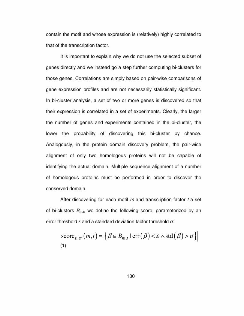
130
contain the motif and whose expression is (relatively) highly correlated to
that of the transcription factor.
It is important to explain why we do not use the selected subset of
genes directly and we instead go a step further computing bi-clusters for
those genes. Correlations are simply based on pair-wise comparisons of
gene expression profiles and are not necessarily statistically significant.
In bi-cluster analysis, a set of two or more genes is discovered so that
their expression is correlated in a set of experiments. Clearly, the larger
the number of genes and experiments contained in the bi-cluster, the
lower the probability of discovering this bi-cluster by chance.
Analogously, in the protein domain discovery problem, the pair-wise
alignment of only two homologous proteins will not be capable of
identifying the actual domain. Multiple sequence alignment of a number
of homologous proteins must be performed in order to discover the
conserved domain.
After discovering for each motif m and transcription factor t a set
of bi-clusters Bm,t, we define the following score, parameterized by an
error threshold ε and a standard deviation factor threshold σ:
( ) ( ) ( ){ }, ,score , | err stdm tm t Bε σ β β ε β σ= ∈ < ∧ >
(1)
131
In other words, the score is simply the number of bi-clusters
satisfying the constraints. Given a motif m, the transcription factors are
ranked according to their score in order to obtain the n-best predictions.
5.3 Results
5.3.1 Dataset
The dataset we used comprised 23,000 Arabidopsis genes and
their expression in a total of 92 experiments, 79 of which were obtained
by combining replicates of microarray experiments available at
AtGenExpress9, and the remaining 13 experiments from Birnbaum et al.
(2003). Of these genes we kept only the relatively highly expressed
genes, a total of 4,702 genes. For validation we used transcription
factors and their experimentally validated binding sites shown in Table
11 downloaded from the PLACE database10. Special nucleotide codes
appearing in these binding sites are explained in Table 12. A list of
Arabidopsis transcription factors was downloaded from the AGRIS
9 http://arabidopsis.org/info/expression/ATGenExpress.jsp
10 http://www.dna.affrc.go.jp/PLACE/
132
database11. Of the 1,619 transcription factors, only 223 were highly
expressed in our dataset.
5.3.2 Testing
We used the method developed in the previous section in order to
predict for each motif m a set of transcription factors that potentially bind
to that motif. The transcription factors were ranked using the score
introduced in equation (1). We compared the performance of the scoring
scheme with a simple correlation-based score, which is the average
correlation of the genes in set Gm,t to the transcription factor t:
( ),
,
1c- score , ( , )
m t
g t
m t g G
m t corr x xG ∈
= ∑ (2)
where xg is the expression vector of gene g and xt is the expression
vector of transcription factor t.
The results are summarized in Figure 26. Each point in the figure
represents the percentage of correct transcription factor/binding site pair
recovered by each scoring scheme within the n-top predictions, where n
ranges from 5 to 30.
11 http://arabidopsis.med.ohio-state.edu/AtTFDB/
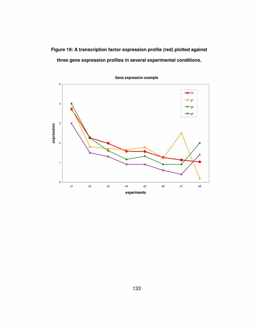
133
Figure 19: A transcription factor expression profile (red) plotted against
three gene expression profiles in several experimental conditions.
Gene expression example
0
1
2
3
4
5
e1 e2 e3 e4 e5 e6 e7 e8
experiments
ex
pre
ss
ion
TF
g1
g2
g3
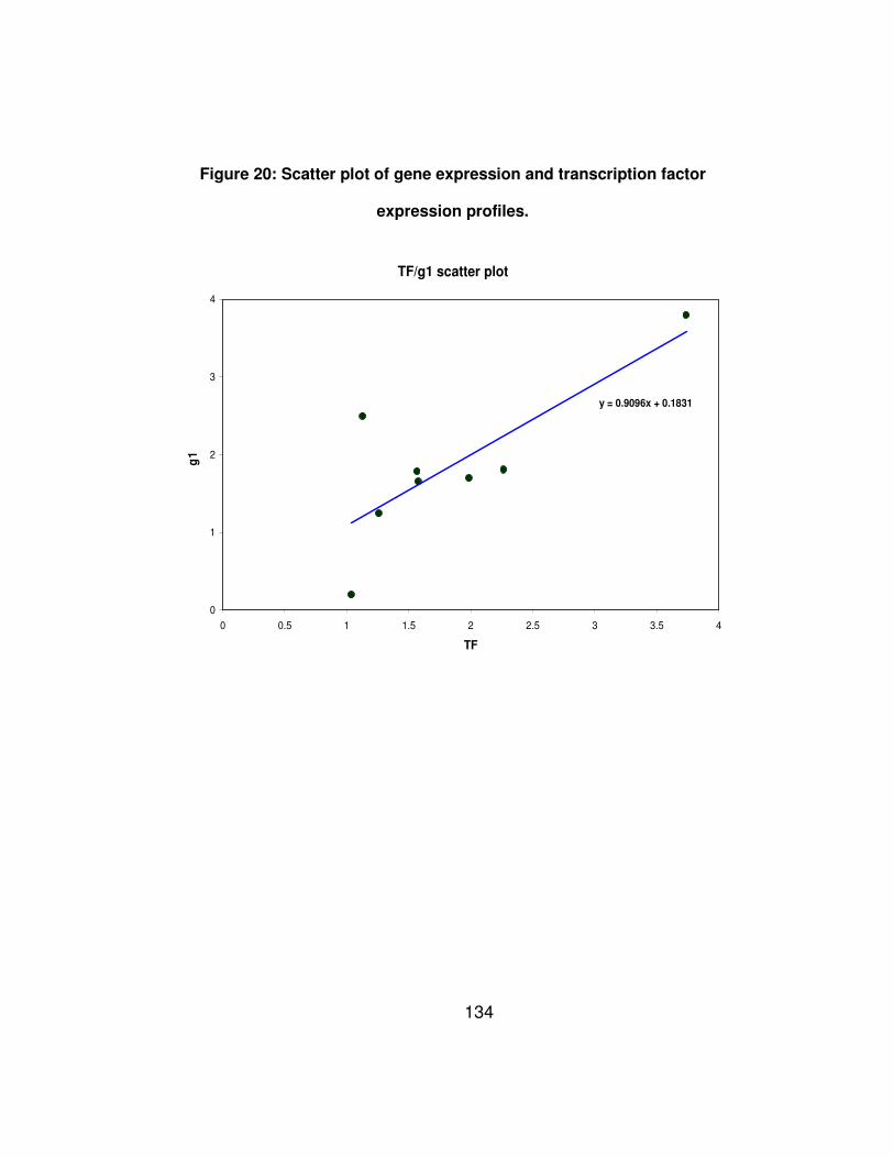
134
Figure 20: Scatter plot of gene expression and transcription factor
expression profiles.
TF/g1 scatter plot
y = 0.9096x + 0.1831
0
1
2
3
4
0 0.5 1 1.5 2 2.5 3 3.5 4
TF
g1
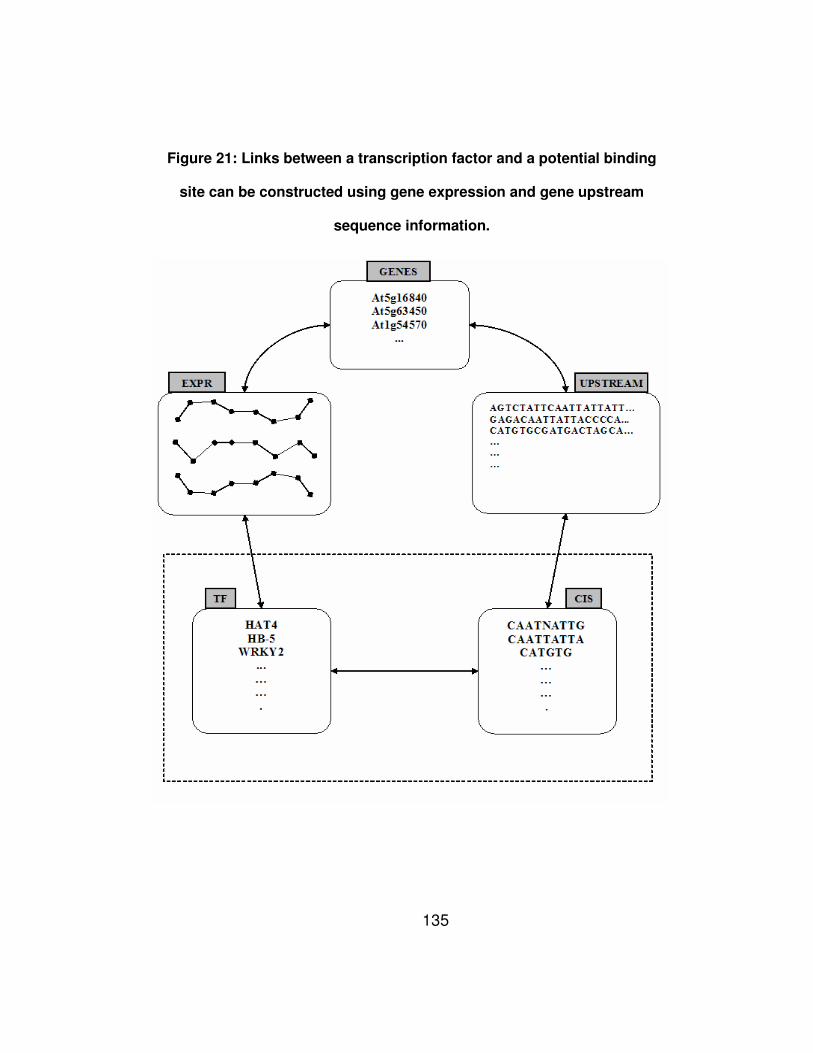
135
Figure 21: Links between a transcription factor and a potential binding
site can be constructed using gene expression and gene upstream
sequence information.
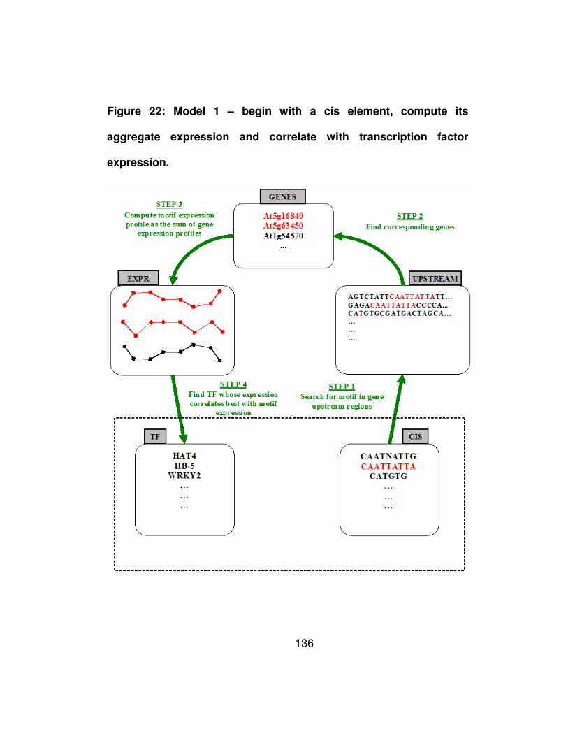
136
Figure 22: Model 1 – begin with a cis element, compute its
aggregate expression and correlate with transcription factor
expression.
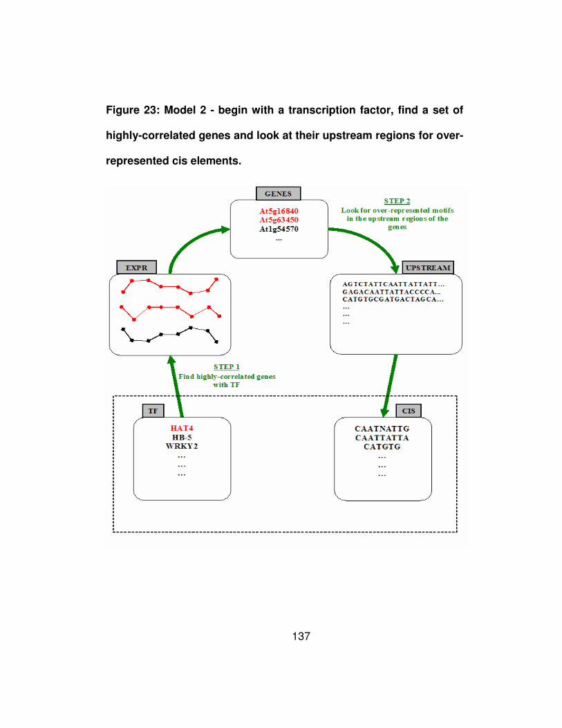
137
Figure 23: Model 2 - begin with a transcription factor, find a set of
highly-correlated genes and look at their upstream regions for over-
represented cis elements.
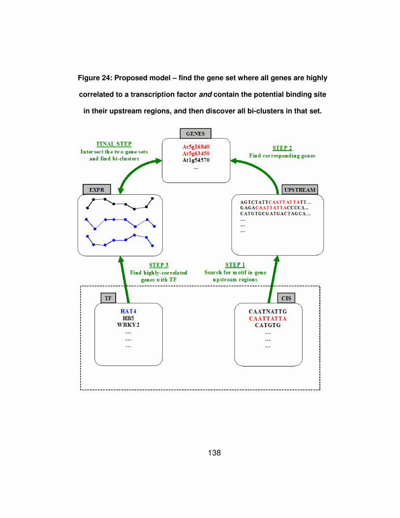
138
Figure 24: Proposed model – find the gene set where all genes are highly
correlated to a transcription factor and contain the potential binding site
in their upstream regions, and then discover all bi-clusters in that set.
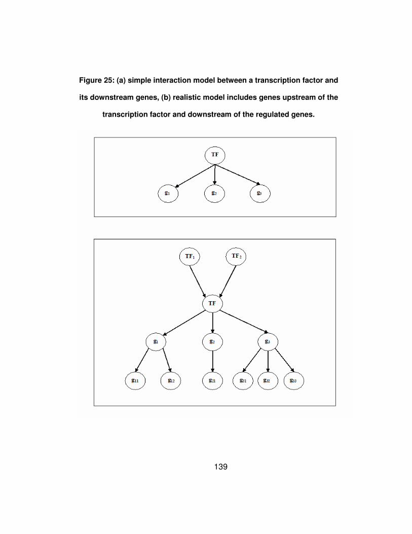
139
Figure 25: (a) simple interaction model between a transcription factor and
its downstream genes, (b) realistic model includes genes upstream of the
transcription factor and downstream of the regulated genes.
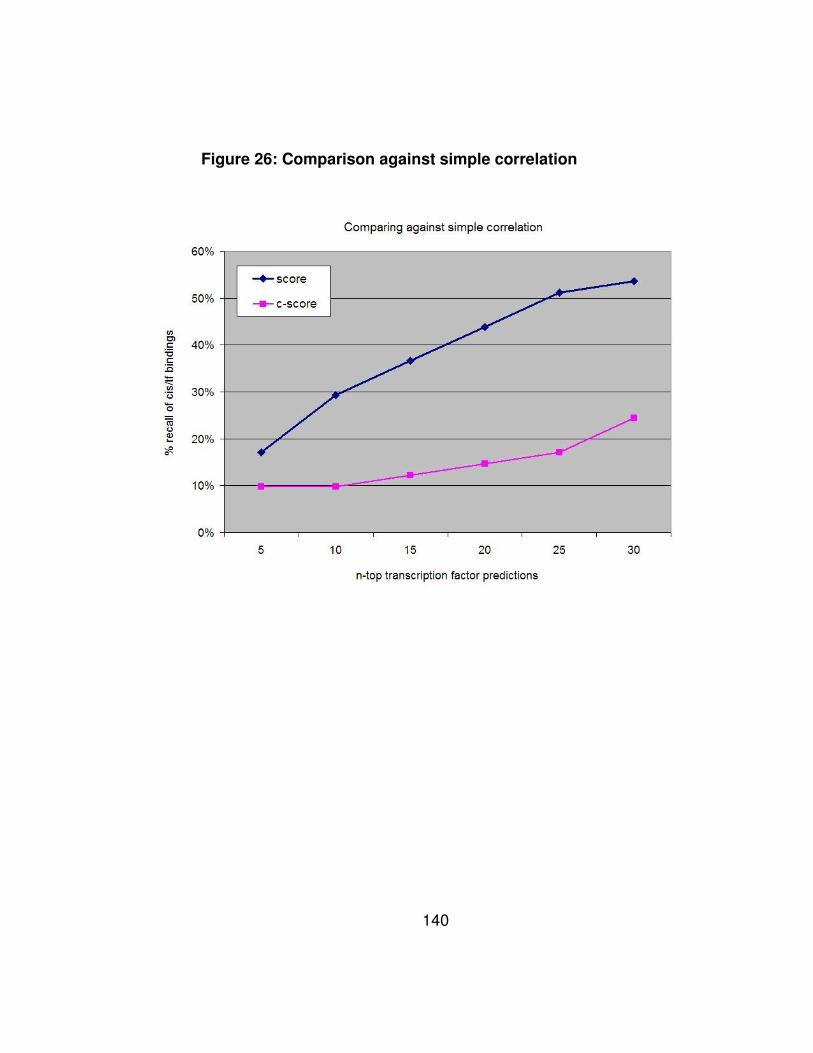
140
Figure 26: Comparison against simple correlation
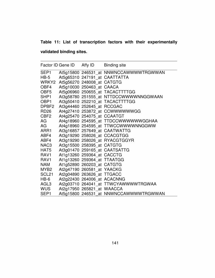
141
Table 11: List of transcription factors with their experimentally
validated binding sites.
Factor ID Gene ID Affy ID Binding site
SEP1 At5g15800 246531_at NNWNCCAWWWWTRGWWAN HB-5 At5g65310 247191_at CAATTATTA WRKY2 At5g56270 248008_at CATGTG OBF4 At5g10030 250463_at CAACA OBF5 At5g06960 250655_at TACACTTTTGG SHP1 At3g58780 251555_at NTTDCCWWWWNNGGWAAN OBP1 At3g50410 252210_at TACACTTTTGG DPBF2 At3g44460 252645_at RCCGAC RD26 At4g27410 253872_at CCWWWWWWGG CBF2 At4g25470 254075_at CCAATGT AG At4g18960 254595_at TTDCCWWWWWWGGHAA AG At4g18960 254595_at TTWCCWWWWNNGGWW ARR1 At3g16857 257649_at CAATWATTG ABF4 At3g19290 258026_at CCACGTGG ABF4 At3g19290 258026_at RYACGTGGYR NAC3 At3g15500 258395_at CATGTG HAT5 At3g01470 259165_at CAATSATTG RAV1 At1g13260 259364_at CACCTG RAV1 At1g13260 259364_at TTAATGG NAM At1g52890 260203_at CATGTG MYB2 At2g47190 260581_at YAACKG SCL21 At2g04890 263626_at TTGACC HB-6 At2g22430 264006_at ACACNNG AGL3 At2g03710 264041_at TTWCYAWWWWTRGWAA WUS At2g17950 265821_at WAACCA SEP1 At5g15800 246531_at NNWNCCAWWWWTRGWWAN
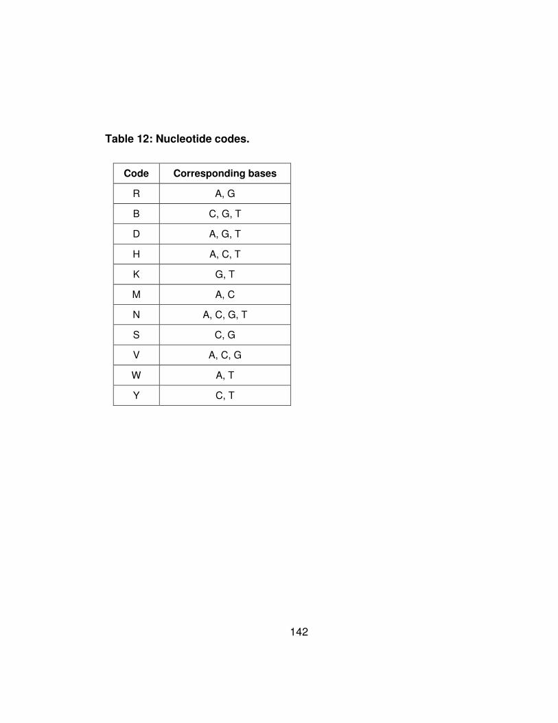
142
Table 12: Nucleotide codes.
Code Corresponding bases
R A, G
B C, G, T
D A, G, T
H A, C, T
K G, T
M A, C
N A, C, G, T
S C, G
V A, C, G
W A, T
Y C, T
143
6 Future work
In future work, we are planning to extend the work on horizontal
gene transfer in order to be able to perform phylogenetic placement of
genes and gene fragments of unknown origin. This will enable the
classification of environmental samples.
Of particular interest is the analysis of repetitive non-coding
elements that in the human genome in order to discover insertion and
deletion events and therefore trace their evolutionary history. Since these
elements are also transcribed into mRNA, we are planning to investigate
a potential regulatory role for these elements.
Finally, we are currently applying the bi-cluster discovery
technique presented in chapter 5 in order to identify upstream regulators
of transcription factors in Arabidopsis and ultimately generate testable
hypotheses in the form of putative regulatory networks between
transcription factors.
144
Bibliography
1. Brazma, A., et al., Approaches to the automatic discovery of
patterns in biosequences. J Comput Biol, 1998. 5(2): p. 279-305.
2. Lawrence, C.E., et al., Detecting subtle sequence signals: a Gibbs
sampling strategy for multiple alignment. Science, 1993.
262(5131): p. 208-14.
3. Neuwald, A.F., J.S. Liu, and C.E. Lawrence, Gibbs motif
sampling: detection of bacterial outer membrane protein repeats.
Protein Sci, 1995. 4(8): p. 1618-32.
4. Bailey, T.L. and C. Elkan, Unsupervised Learning of Multiple
Motifs in Biopolymers Using Expectation Maximization. Mach.
Learn., 1995. 21(1-2): p. 51-80.
5. Roth, F.P., et al., Finding DNA regulatory motifs within unaligned
noncoding sequences clustered by whole-genome mRNA
quantitation. Nat Biotechnol, 1998. 16(10): p. 939-45.
145
6. Altschul, S.F., et al., Gapped BLAST and PSI-BLAST: a new
generation of protein database search programs. Nucleic Acids
Res, 1997. 25(17): p. 3389-402.
7. Hertz, G.Z. and G.D. Stormo, Identifying DNA and protein patterns
with statistically significant alignments of multiple sequences.
Bioinformatics, 1999. 15(7-8): p. 563-77.
8. Rocke, E. and M. Tompa, An algorithm for finding novel gapped
motifs in DNA sequences. Proceedings of the second annual
international conference on Computational molecular biology.
1998, New York, New York, United States: ACM Press. 228-233.
9. Wolfertstetter, F., et al., Identification of functional elements in
unaligned nucleic acid sequences by a novel tuple search
algorithm. Comput Appl Biosci, 1996. 12(1): p. 71-80.
10. Rigoutsos, I. and A. Floratos, Combinatorial pattern discovery in
biological sequences: The TEIRESIAS algorithm. Bioinformatics,
1998. 14(1): p. 55-67.
11. Rigoutsos, I. and A. Floratos, Motif discovery without alignment or
enumeration (extended abstract). Proceedings of the second
annual international conference on Computational molecular
biology. 1998, New York, New York, United States: ACM Press.
221-227.
146
12. Hart, R., et al., Systematic and automated discovery of patterns in
PROSITE families. Proceedings of the fourth annual international
conference on Computational molecular biology. 2000, Tokyo,
Japan: ACM Press. 147-154.
13. McCreight, E.M., A Space-Economical Suffix Tree Construction
Algorithm. J. ACM, 1976. 23(2): p. 262-272.
14. Ukkonen, E., On-line construction of suffix trees. Algorithmica,
1995. 14(3): p. 249-260.
15. Gusfield, D., Algorithms on Strings, Trees and Sequences:
Computer Science and Computational Biology. 1997, New York:
Cambridge University Press.
16. Lonardi, S., Global detectors of unusual words: design,
implementation, and applications to pattern discovery in
biosequences. 2001. p. 167.
17. Apostolico, A., M.E. Bock, and S. Lonardi, Monotony of surprise
and large-scale quest for unusual words. J Comput Biol, 2003.
10(3-4): p. 283-311.
18. Levy, S., et al., Xlandscape: the graphical display of word
frequencies in sequences. Bioinformatics, 1998. 14(1): p. 74-80.
19. Manber, U. and G. Myers. Suffix Arrays: A New Method for On-
line String Searches. in Proceedings of the first annual ACM-SIAM
147
symposium on Discrete algorithms. 1990. San Francisco,
California, United States.
20. Vilo, J., Pattern Discovery in Biosequences, in Computer Science.
2002, University of Helsinki.
21. Giegerich, R. and S. Kurtz, A comparison of imperative and purely
functional suffix tree constructions. Selected papers of ESOP '94,
the 5th European symposium on Programming. 1995, Edinburgh,
United Kingdom: Elsevier Science Publishers B. V. 187-218.
22. Giegerich, R., S. Kurtz, and J. Stoye, Efficient Implementation of
Lazy Suffix Trees. Proceedings of the 3rd International Workshop
on Algorithm Engineering. 1999: Springer-Verlag. 30-42.
23. Pearl, J., Probabilistic Reasoning in Intelligent Systems: Networks
of Plausible Inference. 1988: Morgan Kaufmann Publishers Inc.
552.
24. Heckerman, D., A tutorial on learning with Bayesian networks.
Proceedings of the NATO Advanced Study Institute on Learning in
graphical models. 1998, Erice, Italy: Kluwer Academic Publishers.
301-354.
25. Koller, D. and A. Pfeffer, Probabilistic frame-based systems.
Proceedings of the fifteenth national/tenth conference on Artificial
intelligence/Innovative applications of artificial intelligence. 1998,
148
Madison, Wisconsin, United States: American Association for
Artificial Intelligence. 580-587.
26. Getoor, L.C., Learning statistical models from relational data.
2002. p. 206.
27. Collins, M., R.E. Schapire, and Y. Singer, Logistic Regression,
AdaBoost and Bregman Distances. Mach. Learn., 2002. 48(1-3):
p. 253-285.
28. Schapire, R.E. and Y. Singer, Improved boosting algorithms using
confidence-rated predictions. Proceedings of the eleventh annual
conference on Computational learning theory. 1998, Madison,
Wisconsin, United States: ACM Press. 80-91.
29. Meir, R. and G. Ratsch, An introduction to boosting and
leveraging, in Advanced lectures on machine learning. 2003,
Springer-Verlag New York, Inc. p. 118-183.
30. Lebanon, G. and J.D. Lafferty, Cranking: Combining Rankings
Using Conditional Probability Models on Permutations.
Proceedings of the Nineteenth International Conference on
Machine Learning. 2002: Morgan Kaufmann Publishers Inc. 363-
370.
149
31. Har-Peled, S., D. Roth, and D. Zimak. Constraint classification:A
new approach to multiclass classification and ranking. in NIPS.
2002: MIT Press.
32. Cristianini, N. and J. Shawe-Taylor, An introduction to Support
Vector Machines. 2000: Cambridge University Press.
33. Dekel, O., J. Keshet, and Y. Singer, Large margin hierarchical
classification. Proceedings of the twenty-first international
conference on Machine learning. 2004, Banff, Alberta, Canada:
ACM Press. 27.
34. Ben-Hur, A., et al., Support vector clustering. J. Mach. Learn.
Res., 2002. 2: p. 125-137.
35. Scholkopf, B., et al., Estimating the support of a high-dimensional
distribution. Neural Comput, 2001. 13(7): p. 1443-71.
36. Tsochantaridis, I., et al., Support vector machine learning for
interdependent and structured output spaces. Proceedings of the
twenty-first international conference on Machine learning. 2004,
Banff, Alberta, Canada: ACM Press. 104.
37. Altun, Y., T. Hofmann, and A.J. Smola, Gaussian process
classification for segmenting and annotating sequences.
Proceedings of the twenty-first international conference on
Machine learning. 2004, Banff, Alberta, Canada: ACM Press. 4.
150
38. Avery, O.T., C.M. MacLeod, and M. McCarty, Studies on the
chemical nature of the substance inducing transformation of
pneumococcal types. Induction of transformation by a
desoxyribonucleic acid fraction isolated from Pneumococcus type
III. 1944. Mol Med, 1995. 1(4): p. 344-65.
39. Gray, M.W., Evolution of organellar genomes. Curr Opin Genet
Dev, 1999. 9(6): p. 678-87.
40. Lang, B.F., M.W. Gray, and G. Burger, Mitochondrial genome
evolution and the origin of eukaryotes. Annu Rev Genet, 1999. 33:
p. 351-97.
41. Martin, W. and R.G. Herrmann, Gene transfer from organelles to
the nucleus: how much, what happens, and Why? Plant Physiol,
1998. 118(1): p. 9-17.
42. Smith, M.W., D.F. Feng, and R.F. Doolittle, Evolution by
acquisition: the case for horizontal gene transfers. Trends
Biochem Sci, 1992. 17(12): p. 489-93.
43. Syvanen, M., Cross-species gene transfer; implications for a new
theory of evolution. J Theor Biol, 1985. 112(2): p. 333-43.
44. Doolittle, W.F., Phylogenetic classification and the universal tree.
Science, 1999. 284(5423): p. 2124-9.
151
45. Groisman, E.A., M.H. Saier, Jr., and H. Ochman, Horizontal
transfer of a phosphatase gene as evidence for mosaic structure
of the Salmonella genome. Embo J, 1992. 11(4): p. 1309-16.
46. Medigue, C., et al., Evidence for horizontal gene transfer in
Escherichia coli speciation. J Mol Biol, 1991. 222(4): p. 851-6.
47. Aravind, L., et al., Evidence for massive gene exchange between
archaeal and bacterial hyperthermophiles. Trends Genet, 1998.
14(11): p. 442-4.
48. Nelson, K.E., et al., Evidence for lateral gene transfer between
Archaea and bacteria from genome sequence of Thermotoga
maritima. Nature, 1999. 399(6734): p. 323-9.
49. Doolittle, W.F. and J.M. Logsdon, Jr., Archaeal genomics: do
archaea have a mixed heritage? Curr Biol, 1998. 8(6): p. R209-11.
50. Koonin, E.V., et al., Comparison of archaeal and bacterial
genomes: computer analysis of protein sequences predicts novel
functions and suggests a chimeric origin for the archaea. Mol
Microbiol, 1997. 25(4): p. 619-37.
51. Makarova, K.S., et al., Comparative genomics of the Archaea
(Euryarchaeota): evolution of conserved protein families, the
stable core, and the variable shell. Genome Res, 1999. 9(7): p.
608-28.
152
52. Paulsen, I.T., et al., Role of mobile DNA in the evolution of
vancomycin-resistant Enterococcus faecalis. Science, 2003.
299(5615): p. 2071-4.
53. Weigel, L.M., et al., Genetic analysis of a high-level vancomycin-
resistant isolate of Staphylococcus aureus. Science, 2003.
302(5650): p. 1569-71.
54. Syvanen, M. and C. Kado, Horizontal Gene Transfer. 2002, San
Diego, CA, USA: Academic Press.
55. Syvanen, M., Horizontal gene transfer: evidence and possible
consequences. Annu Rev Genet, 1994. 28: p. 237-61.
56. Koonin, E.V., K.S. Makarova, and L. Aravind, Horizontal gene
transfer in prokaryotes: quantification and classification. Annu Rev
Microbiol, 2001. 55: p. 709-42.
57. Naito, T., K. Kusano, and I. Kobayashi, Selfish behavior of
restriction-modification systems. Science, 1995. 267(5199): p.
897-9.
58. Kobayashi, I., et al., Shaping the genome--restriction-modification
systems as mobile genetic elements. Curr Opin Genet Dev, 1999.
9(6): p. 649-56.
153
59. Ochman, H., J.G. Lawrence, and E.A. Groisman, Lateral gene
transfer and the nature of bacterial innovation. Nature, 2000.
405(6784): p. 299-304.
60. Ikemura, T., Codon usage and tRNA content in unicellular and
multicellular organisms. Mol Biol Evol, 1985. 2(1): p. 13-34.
61. Lawrence, J.G. and H. Ochman, Molecular archaeology of the
Escherichia coli genome. Proc Natl Acad Sci U S A, 1998. 95(16):
p. 9413-7.
62. Karlin, S., J. Mrazek, and A.M. Campbell, Codon usages in
different gene classes of the Escherichia coli genome. Mol
Microbiol, 1998. 29(6): p. 1341-55.
63. Karlin, S. and C. Burge, Dinucleotide relative abundance
extremes: a genomic signature. Trends Genet, 1995. 11(7): p.
283-90.
64. Karlin, S., J. Mrazek, and A.M. Campbell, Compositional biases of
bacterial genomes and evolutionary implications. J Bacteriol,
1997. 179(12): p. 3899-913.
65. Karlin, S. and J. Mrazek, What drives codon choices in human
genes? J Mol Biol, 1996. 262(4): p. 459-72.
66. Pride, D.T. and M.J. Blaser, Identification of horizontally acquired
genetic elements in Helicobacter pylori and other
154
prokaryotesusing oligonucleotide difference analysis. Genome
Letters, 2002. 1: p. 2-15.
67. Hooper, S.D. and O.G. Berg, Detection of genes with atypical
nucleotide sequence in microbial genomes. J Mol Evol, 2002.
54(3): p. 365-75.
68. Sandberg, R., et al., Capturing whole-genome characteristics in
short sequences using a naive Bayesian classifier. Genome Res,
2001. 11(8): p. 1404-9.
69. Hayes, W.S. and M. Borodovsky, How to interpret an anonymous
bacterial genome: machine learning approach to gene
identification. Genome Res, 1998. 8(11): p. 1154-71.
70. Nakamura, Y., et al., Biased biological functions of horizontally
transferred genes in prokaryotic genomes. Nat Genet, 2004.
36(7): p. 760-6.
71. Borodovsky, M. and J.D. McIninch, GENMARK: Parallel gene
recognition for both DNA strands. Computers & Chemistry, 1993.
17: p. 123-134.
72. Campbell, A., J. Mrazek, and S. Karlin, Genome signature
comparisons among prokaryote, plasmid, and mitochondrial DNA.
Proc Natl Acad Sci U S A, 1999. 96(16): p. 9184-9.
155
73. Garcia-Vallve, S., et al., HGT-DB: a database of putative
horizontally transferred genes in prokaryotic complete genomes.
Nucleic Acids Res, 2003. 31(1): p. 187-9.
74. Ragan, M.A., On surrogate methods for detecting lateral gene
transfer. FEMS Microbiol Lett, 2001. 201(2): p. 187-91.
75. Ragan, M.A. and R.L. Charlebois, Distributional profiles of
homologous open reading frames among bacterial phyla:
implications for vertical and lateral transmission. Int J Syst Evol
Microbiol, 2002. 52(Pt 3): p. 777-87.
76. Jain, R., M.C. Rivera, and J.A. Lake, Horizontal gene transfer
among genomes: the complexity hypothesis. Proc Natl Acad Sci U
S A, 1999. 96(7): p. 3801-6.
77. Brochier, C., H. Philippe, and D. Moreira, The evolutionary history
of ribosomal protein RpS14: horizontal gene transfer at the heart
of the ribosome. Trends Genet, 2000. 16(12): p. 529-33.
78. Doolittle, R.F. and J. Handy, Evolutionary anomalies among the
aminoacyl-tRNA synthetases. Curr Opin Genet Dev, 1998. 8(6): p.
630-6.
79. Wolf, Y.I., et al., Evolution of aminoacyl-tRNA synthetases--
analysis of unique domain architectures and phylogenetic trees
156
reveals a complex history of horizontal gene transfer events.
Genome Res, 1999. 9(8): p. 689-710.
80. Woese, C.R., et al., Aminoacyl-tRNA synthetases, the genetic
code, and the evolutionary process. Microbiol Mol Biol Rev, 2000.
64(1): p. 202-36.
81. Tsirigos, A. and I. Rigoutsos, A new computational method for the
detection of horizontal gene transfer events. Nucleic Acids Res,
2005. 33(3): p. 922-33.
82. Chang, C.-C. and C.-J. Lin, LIBSVM: A library for support vector
machines. Available online:
http://www.csie.ntu.edu.tw/~cjlin/libsvm. 2001.
83. Novotny, J., et al., In silico structural and functional analysis of the
human cytomegalovirus (HHV5) genome. J Mol Biol, 2001.
310(5): p. 1151-66.
84. Rigoutsos, I., et al., In silico pattern-based analysis of the human
cytomegalovirus genome. J Virol, 2003. 77(7): p. 4326-44.
85. Murphy, E., et al., Reevaluation of human cytomegalovirus coding
potential. Proc Natl Acad Sci U S A, 2003. 100(23): p. 13585-90.
86. Chee, M.S., et al., Analysis of the protein-coding content of the
sequence of human cytomegalovirus strain AD169. Curr Top
Microbiol Immunol, 1990. 154: p. 125-69.
157
87. Roizman, B. and P.E. Pellett, The Family Herpesviridae: A Brief
Introduction. 2001: Lippincott Williams & Wilkins.
88. Aridor, M. and L.A. Hannan, Traffic jam: a compendium of human
diseases that affect intracellular transport processes. Traffic,
2000. 1(11): p. 836-51.
89. Aridor, M. and L.A. Hannan, Traffic jams II: an update of diseases
of intracellular transport. Traffic, 2002. 3(11): p. 781-90.
90. Mellman, I., Endocytosis and molecular sorting. Annu Rev Cell
Dev Biol, 1996. 12: p. 575-625.
91. Bryant, D.M. and J.L. Stow, The ins and outs of E-cadherin
trafficking. Trends Cell Biol, 2004. 14(8): p. 427-34.
92. Nakai, K., Protein sorting signals and prediction of subcellular
localization. Adv Protein Chem, 2000. 54: p. 277-344.
93. Emanuelsson, O., Predicting protein subcellular localisation from
amino acid sequence information. Brief Bioinform, 2002. 3(4): p.
361-76.
94. Schneider, G. and U. Fechner, Advances in the prediction of
protein targeting signals. Proteomics, 2004. 4(6): p. 1571-1580.
95. Boden, M. and J. Hawkins, Prediction of subcellular localization
using sequence-biased recurrent networks. Bioinformatics, 2005.
21(10): p. 2279-2286.
158
96. Chen, Y.J., et al., Secreted protein prediction system combining
CJ-SPHMM, TMHMM, and PSORT. Mammalian Genome, 2003.
14(12): p. 859-865.
97. Nair, R. and B. Rost, Mimicking cellular sorting improves
prediction of subcellular localization. Journal Of Molecular Biology,
2005. 348(1): p. 85-100.
98. Zhang, Z.M. and W.J. Henzel, Signal peptide prediction based on
analysis of experimentally verified cleavage sites. Protein
Science, 2004. 13(10): p. 2819-2824.
99. Small, I., et al., Predotar: A tool for rapidly screening proteomes
for N-terminal targeting sequences. Proteomics, 2004. 4(6): p.
1581-1590.
100. Hiller, K., et al., PrediSi: prediction of signal peptides and their
cleavage positions. Nucleic Acids Research, 2004. 32: p. W375-
W379.
101. Heddad, A., M. Brameier, and R.M. MacCallum, Evolving regular
expression-based sequence classifiers for protein nuclear
localisation, in Applications Of Evolutionary Computing. 2004. p.
31-40.
159
102. Bendtsen, J.D., et al., Improved prediction of signal peptides:
SignalP 3.0. Journal Of Molecular Biology, 2004. 340(4): p. 783-
795.
103. Nakashima, H. and K. Nishikawa, Discrimination of intracellular
and extracellular proteins using amino acid composition and
residue-pair frequencies. J Mol Biol, 1994. 238(1): p. 54-61.
104. Gao, Q.B., et al., Prediction of protein subcellular location using a
combined feature of sequence. Febs Letters, 2005. 579(16): p.
3444-3448.
105. Garg, A., M. Bhasin, and G.P.S. Raghava, Support vector
machine-based method for subcellular localization of human
proteins using amino acid compositions, their order, and similarity
search. Journal Of Biological Chemistry, 2005. 280(15): p. 14427-
14432.
106. Park, K.J. and M. Kanehisa, Prediction of protein subcellular
locations by support vector machines using compositions of amino
acids and amino acid pairs. Bioinformatics, 2003. 19(13): p. 1656-
1663.
107. Bhasin, M. and G.P.S. Raghava, ESLpred: SVM-based method
for subcellular localization of eukaryotic proteins using dipeptide
160
composition and PSI-BLAST. Nucleic Acids Research, 2004. 32:
p. W414-W419.
108. Cai, Y.D. and K.C. Chou, Nearest neighbour algorithm for
predicting protein subcellular location by combining functional
domain composition and pseudo-amino acid composition.
Biochemical And Biophysical Research Communications, 2003.
305(2): p. 407-411.
109. Cai, Y.D. and K.C. Chou, Predicting subcellular localization of
proteins in a hybridization space. Bioinformatics, 2004. 20(7): p.
1151-1156.
110. Xiao, X., et al., Using complexity measure factor to predict protein
subcellular location. Amino Acids, 2005. 28(1): p. 57-61.
111. Huang, Y. and Y. Li, Prediction of protein subcellular locations
using fuzzy k-NN method. Bioinformatics, 2004. 20(1): p. 21-28.
112. Reczko, M. and A. Hatzigeorgiou, Prediction of the subcellular
localization of eukaryotic proteins using sequence signals and
composition. Proteomics, 2004. 4(6): p. 1591-1596.
113. Nair, R. and B. Rost, LOCnet and LOCtarget: sub-cellular
localization for structural genomics targets. Nucleic Acids
Research, 2004. 32: p. W517-W521.
161
114. Rigoutsos, I. and A. Floratos, Combinatorial pattern discovery in
biological sequences: the TEIRESIAS algorithm (vol 14, pg 55,
1998). Bioinformatics, 1998. 14(2): p. 229-229.
115. Furey, T.S., et al., Support vector machine classification and
validation of cancer tissue samples using microarray expression
data. Bioinformatics, 2000. 16(10): p. 906-14.
116. Vapnik, V.N., The Nature of Statistical Learning Theory. 2 ed.
1999: Springer. 314.
117. Cristianini, N. and J. Shawe-Taylor, An Introduction to Support
Vector Machines and Other Kernel-based Learning Methods. 1
ed. 2000: Cambridge University Press. 189.
118. Chen, Y.-W. and C.-J. Lin, Combining SVMs with various feature
selection strategies., in Feature extraction, foundations and
applications. 2005, to be published.
119. Chen, Y.-W., Combining SVMs with various feature selection
strategies, in Department of Computer Science and Information
Engineering. 2005, National Taiwan University.
120. Buhler, J. and M. Tompa, Finding motifs using random
projections. J Comput Biol, 2002. 9(2): p. 225-42.
162
121. Pevzner, P.A. and S.H. Sze, Combinatorial approaches to finding
subtle signals in DNA sequences. Proc Int Conf Intell Syst Mol
Biol, 2000. 8: p. 269-78.
122. Keich, U. and P.A. Pevzner, Finding motifs in the twilight zone.
Bioinformatics, 2002. 18(10): p. 1374-81.
123. Gelfand, M.S., E.V. Koonin, and A.A. Mironov, Prediction of
transcription regulatory sites in Archaea by a comparative
genomic approach. Nucleic Acids Res, 2000. 28(3): p. 695-705.
124. GuhaThakurta, D. and G.D. Stormo, Identifying target sites for
cooperatively binding factors. Bioinformatics, 2001. 17(7): p. 608-
21.
125. Liu, X., D.L. Brutlag, and J.S. Liu, BioProspector: discovering
conserved DNA motifs in upstream regulatory regions of co-
expressed genes. Pac Symp Biocomput, 2001: p. 127-38.
126. Marsan, L. and M.F. Sagot, Algorithms for extracting structured
motifs using a suffix tree with an application to promoter and
regulatory site consensus identification. J Comput Biol, 2000. 7(3-
4): p. 345-62.
127. van Helden, J., A.F. Rios, and J. Collado-Vides, Discovering
regulatory elements in non-coding sequences by analysis of
spaced dyads. Nucleic Acids Res, 2000. 28(8): p. 1808-18.
163
128. Eskin, E. and P.A. Pevzner, Finding composite regulatory patterns
in DNA sequences. Bioinformatics, 2002. 18 Suppl 1: p. S354-63.
129. Sagot, M.-F., Spelling Approximate Repeated or Common Motifs
Using a Suffix Tree. Proceedings of the Third Latin American
Symposium on Theoretical Informatics. 1998: Springer-Verlag.
374-390.
130. Zhang, M.Q., Promoter analysis of co-regulated genes in the
yeast genome. Comput Chem, 1999. 23(3-4): p. 233-50.
131. Vilo, J. and K. Kivinen, Regulatory sequence analysis: application
to the interpretation of gene expression. Eur
Neuropsychopharmacol, 2001. 11(6): p. 399-411.
132. Ohler, U. and H. Niemann, Identification and analysis of
eukaryotic promoters: recent computational approaches. Trends
Genet, 2001. 17(2): p. 56-60.
133. Werner, T., Cluster analysis and promoter modelling as
bioinformatics tools for the identification of target genes from
expression array data. Pharmacogenomics, 2001. 2(1): p. 25-36.
134. Brazma, A., et al., Predicting gene regulatory elements in silico on
a genomic scale. Genome Res, 1998. 8(11): p. 1202-15.
135. Tavazoie, S., et al., Systematic determination of genetic network
architecture. Nat Genet, 1999. 22(3): p. 281-5.
164
136. Sinha, S. and M. Tompa, A statistical method for finding
transcription factor binding sites. Proc Int Conf Intell Syst Mol Biol,
2000. 8: p. 344-54.
137. Wingender, E., et al., The TRANSFAC system on gene
expression regulation. Nucleic Acids Res, 2001. 29(1): p. 281-3.
138. Barash, Y. and N. Friedman, Context-specific Bayesian clustering
for gene expression data. J Comput Biol, 2002. 9(2): p. 169-91.
139. Segal, E., et al., Rich probabilistic models for gene expression.
Bioinformatics, 2001. 17 Suppl 1: p. S243-52.
140. Segal, E., et al., From promoter sequence to expression: a
probabilistic framework. Proceedings of the sixth annual
international conference on Computational biology. 2002,
Washington, DC, USA: ACM Press. 263-272.
141. Segal, E., R. Yelensky, and D. Koller, Genome-wide discovery of
transcriptional modules from DNA sequence and gene
expression. Bioinformatics, 2003. 19 Suppl 1: p. i273-82.
142. Birnbaum, K., P.N. Benfey, and D.E. Shasha, cis
element/transcription factor analysis (cis/TF): a method for
discovering transcription factor/cis element relationships. Genome
Res, 2001. 11(9): p. 1567-73.
165
143. Bussemaker, H.J., H. Li, and E.D. Siggia, Regulatory element
detection using correlation with expression. Nat Genet, 2001.
27(2): p. 167-71.
144. Pilpel, Y., P. Sudarsanam, and G.M. Church, Identifying
regulatory networks by combinatorial analysis of promoter
elements. Nat Genet, 2001. 29(2): p. 153-9.
145. Eisen, M.B., et al., Cluster analysis and display of genome-wide
expression patterns. Proc Natl Acad Sci U S A, 1998. 95(25): p.
14863-8.
146. Wu, L.F., et al., Large-scale prediction of Saccharomyces
cerevisiae gene function using overlapping transcriptional
clusters. Nat Genet, 2002. 31(3): p. 255-65.
147. Ihmels, J., et al., Revealing modular organization in the yeast
transcriptional network. Nat Genet, 2002. 31(4): p. 370-7.
148. Halfon, M.S., et al., Computation-based discovery of related
transcriptional regulatory modules and motifs using an
experimentally validated combinatorial model. Genome Res,
2002. 12(7): p. 1019-28.
149. Tanay, A., R. Sharan, and R. Shamir, Discovering statistically
significant biclusters in gene expression data. Bioinformatics,
2002. 18 Suppl 1: p. S136-44.
166
150. Spellman, P.T., et al., Comprehensive identification of cell cycle-
regulated genes of the yeast Saccharomyces cerevisiae by
microarray hybridization. Mol Biol Cell, 1998. 9(12): p. 3273-97.
151. Weaver, D.C., C.T. Workman, and G.D. Stormo, Modeling
regulatory networks with weight matrices. Pac Symp Biocomput,
1999: p. 112-23.
152. D'Haeseleer, P., et al., Linear modeling of mRNA expression
levels during CNS development and injury. Pac Symp Biocomput,
1999: p. 41-52.
153. Somogyi, R., et al., The gene expression matrix: towards the
extraction of genetic network architectures. Proceedings of the
second world congress on Nonlinear analysts: part 3. 1997,
Athens, Greece: Pergamon Press, Inc. 1815-1824.
154. Akutsu, T., et al., Identification of gene regulatory networks by
strategic gene disruptions and gene overexpressions.
Proceedings of the ninth annual ACM-SIAM symposium on
Discrete algorithms. 1998, San Francisco, California, United
States: Society for Industrial and Applied Mathematics. 695-702.
155. Holmes, I. and W.J. Bruno, Finding regulatory elements using joint
likelihoods for sequence and expression profile data. Proc Int
Conf Intell Syst Mol Biol, 2000. 8: p. 202-10.
167
156. Friedman, N., et al., Using Bayesian networks to analyze
expression data. J Comput Biol, 2000. 7(3-4): p. 601-20.
157. Beer, M.A. and S. Tavazoie, Predicting gene expression from
sequence. Cell, 2004. 117(2): p. 185-98.
158. Segal, E., Rich Probabilistic Models for Genomic Data, in
Computer Science. 2004, Stanford University.